1

Iterative Redeployment of Illumination andSensing (IRIS): Application to STW-SAR

ImagingJay Marble†,∗, Raviv Raich∗, Alfred O. Hero∗

†Night Vision Laboratory, Fort Belvoir, VA 22060∗University of Michigan, Ann Arbor, MI 48109-2122

Abstract— A new technique which we call IterativeRedeployment of Illumination and Sensing (IRIS) isintroduced and applied to See-Through-the-Wall radarimaging. IRIS is applicable to adaptive sensing scenarioswhere the medium is illuminated and measured multipletimes using different illiminator/sensor configurations,e.g.,position, bandwidth, or polarization. These configurationsare adaptively selected to minimize uncertainty in the im-age reconstruction. The IRIS algorithm has the followingfeatures: (1) use of a sparse Bayesian image model thatcaptures the free-space dominated propagation character-istics of interiors of man-made structures such as caves andresidences; (2) iterative reconstruction of both an imageand an image confidence map from the posterior likelihoodin the form of a thresholded Landweber recursion, (3) useof the Bayesian model to predict the best redeploymentconfiguration of the illuminator platform given the currentimage and confidence map. For the STW application weapproximate the forward operator by a matrix formulationof wavenumber migration. A simulated STW applicationis provided that illustrates the IRIS algorithm.

I. I NTRODUCTION

Imaging with See-Through-the-Wall (STW) radar isof high interest to military, homeland security, andsearch-and-rescue operations due to its ability to provideinformation on activities and conditions behind walls.Tracking suspicious individuals, detection of weaponscaches, layout mapping, and fire rescue are examplesof STW applications. For such applications STW radarmust have the following properties: rapid deployment,small (even portable) size, and the ability to performfast image reconstruction from limited angle views.In general, to maximize resolution and signal-to-noiseperformance one should deploy as powerful a radar aspossible, i.e., high transmit energy and long baseline.

This research was partially supported by the Army ResearchOffice, grant number DAAD19-02-1-0262. Authors can be contactedat jamarble,ravivr,hero at umich.edu

However, in military, homeland security, or firefightingapplications, the deployment of bulky or long-baselineSTW radar platforms might entail risks that could com-promise mission objectives or endanger those who aredeploying the radar. In these situations, it is essentialthat the size of the illumination and sensing platformsbe small and that the radar deployment time, e.g., thebaseline of a SAR system, be short. To gain back some ofthe performance lost by downsizing the radar we proposean adaptive deployment strategy that we call iterativeredeployment of illumination and sensing (IRIS). IRISallows one to rapidly learn the propagation environment,adapt the configuration of the radar, e.g., its placementat the exterior of a building, and continuously improvethe image during the deployment process.

One unique characteristic of STW that the IRIS ap-proach exploits is that in man-made structures most ofthe image volume is empty space, i.e., interiors are onlysparsely populated with scatter centers. This allows us toimplement fast image reconstruction and derive an imageconfidence map that measures the degree of uncertaintythat a scatterer exists at any specified location in theimage. Regions of the image with high uncertainty mayneed to be reimaged with a different illumination/sensorconfiguration. The optimal redeployment configuration,e.g., sensor position, can be determined on the flyby choosing the one that would maximize informationgain in interesting regions of the image where scattererconfidence, as predicted by the confidence map, is low.Information gain is computed by placing a virtual emitterin the low confidence region and applying the reciprocityprinciple. This forms the basis for the IRIS approach.

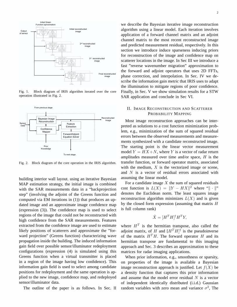
The elements of the IRIS approach are illustrated inFig. 1 and 2. The former figure illustrates the iterationsover the block operation in 2. The algorithm starts withan initial position of the sensor/illuminator and an initialestimate of the image, which could be very crude, e.g.,an all blank image, or could use prior information, e.g.,

2

Fig. 1. Block diagram of IRIS algorithm iterated over the coreoperation illustrated in Fig. 2.

Fig. 2. Block diagram of the core operation in the IRIS algorithm.

building interior wall layout. using an iterative BayesianMAP estimation strategy, the initial image is combinedwith the SAR measurements data in a “backprojectionstep” (involving the adjoint of the Greens function andcomputed via EM iterations in (1)) that produces an up-dated image and an approximate image confidence map(expression (3)). The confidence map is used to selectregions of the image that could not be reconstructed withhigh confidence from the SAR measurements. Featuresextracted from the confidence image are used to estimatelikely positions of scatterers and approximate the ”for-ward projection” (Greens function) characterizing wavepropagation inside the building. The induced informationgain field over possible sensor/illuminator redeploymentconfigurations (expression (4) is simulated using thisGreens function when a virtual transmitter is placedin a region of the image having low confidence). Thisinformation gain field is used to select among candidatepositions for redeployment and the same operation is ap-plied to the new image, confidence map, and redeployedsensor/illuminator data.

The outline of the paper is as follows. In Sec. II

we describe the Bayesian iterative image reconstructionalgorithm using a linear model. Each iteration involvesapplication of a forward channel matrix and an adjointchannel matrix to the most recent reconstructed imageand predicted measurement residual, respectively. In thissection we introduce induce sparseness inducing priorsfor reconstruction of the image and confidence map onscatterer locations in the image. In Sec III we introduce afast ”reverse wavenumber migration” approximation tothe forward and adjoint operators that uses 2D FFTs,phase correction, and interpolation. In Sec. IV we de-scribe the information gain metric that IRIS uses to adaptthe illumination to mitigate regions of poor confidence.Finally, in Sec. V we show simulation results for a STWSAR application and conclude in Sec VI.

II. I MAGE RECONSTRUCTION ANDSCATTERER

PROBABILITY MAPPING

Most image reconstruction approaches can be inter-preted as solutions to a cost function minimization prob-lem, e.g., minimization of the sum of squared residualerrors between the observed measurements and measure-ments synthesized with a candidate reconstructed image.The starting point is the linear vector measurementmodelY = HX+N , whereY is a vector of radar returnamplitudes measured over time and/or space,H is thetransfer function, or forward operator matrix, associatedwith the medium,X is the vectorized image or scene,and N is a vector of residual errors associated withassuming the linear model.

For a candidate imageX the sum of squared residualscost function isL(X) = ‖Y − HX‖2 where “‖ · ‖”denotes the Euclidean norm. The least squares imagereconstruction algorithm minimizesL(X) and is givenby the closed form expression (assuming that matrixHis full column rank)

X = [HT H]†HT Y,

where HT is the hermitian transpose, also called theadjoint matrix, ofH and [HT H]† is the pseudoinverseof the matrix HT H. The forward operatorH and itshermitian transpose are fundamental to this imagingapproach and Sec. 3 describes an approximation to thesematrices for radar imaging applications.

When prior information, e.g., smoothness or sparsity,on properties of the image is available a Bayesianimage reconstruction approach is justified. Letf(X) bea density function that captures this prior informationand assume that the model error residualN is a vectorof independent identically distributed (i.i.d.) Gaussianrandom variables with zero mean and varianceσ2, The

3

maximum a posteriori (MAP) reconstruction maximizesthe posterior densityf(X|Y ) = f(Y |X)f(X)/f(Y ) orequivalently minimizes the objective function

L(X) = ‖Y − HX‖2/(2σ2) + log f(X)

Only in rare cases, e.g., Gaussianf(X), is the minimizerof L(X) available in closed form. However, this MAPreconstruction can always be implemented iterativelyusing the Expectation-Maximization (EM) algorithm [1].As shown in [2] the EM algorithm performs imagereconstruction by iterating two nested operations the ”E”(deconvolution) step and the ”M” (denoising) step:

(E) Z(n) = X(n) + αHT (Y − HX(n)) (1)

(M) X(n+1) = arg minX

(‖Z(n) − X‖2

2σ2+ log f(X)

)

.

A. Sparse Bayesian image model

We adopt a model for the joint image densityf(X)that reflects inherent sparseness (many zero entries inthe vectorX) introduced in [3] for molecular imagingapplications. As we will see this model also yields aconfidence map estimate. Adopting the notationX =[x1, . . . , xP ]T the model isf(X) =

∏Pi=1 g(xi) whereg

is the marginal density

g(x) = (1 − w)δ(x) +wa

2e−a|x| (2)

δ(x) is a dirac delta function (point mass at zero),w ∈ [0, 1], a > 0 are parameters, which are generallyunknown and must be estimated. With this model theEM algorithm (1) gives an M step, which is closed formand is equivalent to applying a soft thresholding functionto each of the variablesZ(n) [3]. Furthermore, thismodel gives an iterative approximation to the posteriorprobability P (xi = 0|Y ) that thei-th pixel is zero [4]:

P (xi = 0|Y ) ≈1−w√2πσ2

e−z2

2σ2

fz(z)(3)

fz(z) =1 − w√2πσ2

e−z2

2σ2 + A(w, a, σ, z) + B(w, a, σ, z),

where

A(w, a, σ, z) =aw

4

(

1 − erf(aσ + z

σ√2

))

ea2

σ2+2az

2 ,

B(w, a, σ, z) =aw

4

(

1 + erf(

zσ− aσ√

2

))

ea2

σ2−2az

2 .

An image of the values ofP (xi = 0|Y ) over allpixel indicesi will be called the “probability map” ofscatterers in the reconstructed image.

Fig. 3. Block diagram of wavenumber migration. The SARmeasurementsY are input to the block at the left of diagram andthe reconstructed imageX is output at the block on the right.

III. R EVERSE MIGRATION APPROXIMATION

The form of the matricesH and HT in the EMiteration (1) will depend on the specific application andmodality used to illuminate and sense the environment.For SAR imaging we develop an approximation tothese matrices that is based on a matrix formulationof wavenumber migration. Wavenumber migration wasfirst developed as a way of imaging seismic data for oilexploration. It was applied to synthetic aperture radarimaging in the early 90s. [5]. Wavenumber migrationis implemented by rebinning the frequency-wavenumberspectrum (Ω−k domain) into a 2D Fourier spectrum plusa correction factor determined by a Stolt interpolation[6].

Wavenumber migration can be interpreted as compo-sition of several operators, which can implemented asa sequence of matrix operations (See block diagram inFig. 3). This gives a compact mathematical form for theimage reconstructionX = ΨY where

Ψ = Q−12 ΦQ1,

and Q1 is a 1D FFT, placing the observations into thefrequency-wavenumber (Ω−k ) space.Q2 is the matriximplementation of a 2D FFT and the phase compensationand Stolt interpolation and are folded into the matrixΦ.The matrixΨ an be identified as an approximation to thepseudo-inverse[HT H]−1HT of the forward operatorH.

The Stolt interpolation is a 1D interpolation betweensampled frequencies in the wavenumber domain. Toimplement this operation as a matrix we start with thesimple two point (linear) interpolator. If we denote theset of observations byy[n, m] wheren corresponds tothe n-th spatial location along the synthetic apertureand m corresponds to them-th transmitted frequency,then the Stolt interpolation can be written asy[n, m] →amy[n, m] + bmy[n[m + 1] for frequency dependentinterpolation coefficientsam, bm:

am =k′

m − km

km+1 − km

, bm =km+1 − k′

m

km+1 − km

corresponding to a vector interpolation of the formY →AY whereA is a sparse matrix. Herekm = 2πfm/c isthe wavenumber at them-th frequency andk′

m is thewavenumber atm-th interpolated frequency.

4

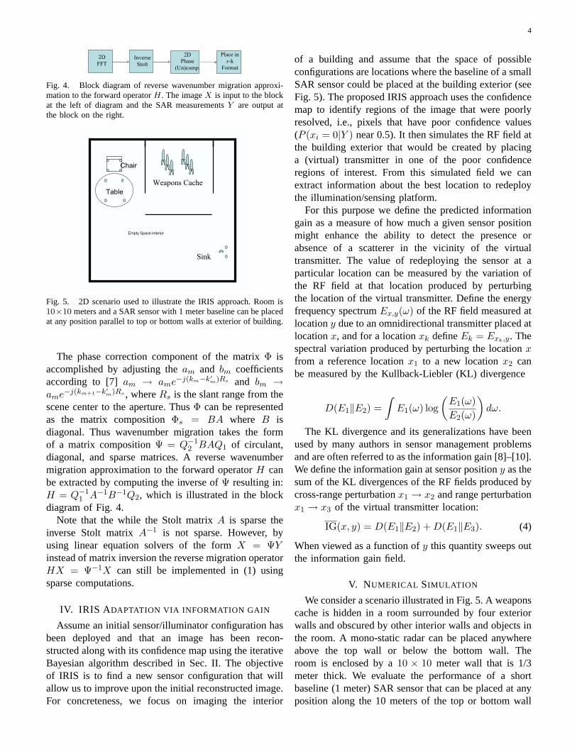
Fig. 4. Block diagram of reverse wavenumber migration approxi-mation to the forward operatorH. The imageX is input to the blockat the left of diagram and the SAR measurementsY are output atthe block on the right.

Fig. 5. 2D scenario used to illustrate the IRIS approach. Room is10×10 meters and a SAR sensor with 1 meter baseline can be placedat any position parallel to top or bottom walls at exterior of building.

The phase correction component of the matrixΦ isaccomplished by adjusting theam and bm coefficientsaccording to [7]am → ame−j(km−k′

m)Rs and bm →

ame−j(km+1−k′

m)Rs , whereRs is the slant range from the

scene center to the aperture. ThusΦ can be representedas the matrix compositionΦs = BA where B isdiagonal. Thus wavenumber migration takes the formof a matrix compositionΨ = Q−1

2 BAQ1 of circulant,diagonal, and sparse matrices. A reverse wavenumbermigration approximation to the forward operatorH canbe extracted by computing the inverse ofΨ resulting in:H = Q−1

1 A−1B−1Q2, which is illustrated in the blockdiagram of Fig. 4.

Note that the while the Stolt matrixA is sparse theinverse Stolt matrixA−1 is not sparse. However, byusing linear equation solvers of the formX = ΨYinstead of matrix inversion the reverse migration operatorHX = Ψ−1X can still be implemented in (1) usingsparse computations.

IV. IRIS A DAPTATION VIA INFORMATION GAIN

Assume an initial sensor/illuminator configuration hasbeen deployed and that an image has been recon-structed along with its confidence map using the iterativeBayesian algorithm described in Sec. II. The objectiveof IRIS is to find a new sensor configuration that willallow us to improve upon the initial reconstructed image.For concreteness, we focus on imaging the interior

of a building and assume that the space of possibleconfigurations are locations where the baseline of a smallSAR sensor could be placed at the building exterior (seeFig. 5). The proposed IRIS approach uses the confidencemap to identify regions of the image that were poorlyresolved, i.e., pixels that have poor confidence values(P (xi = 0|Y ) near 0.5). It then simulates the RF field atthe building exterior that would be created by placinga (virtual) transmitter in one of the poor confidenceregions of interest. From this simulated field we canextract information about the best location to redeploythe illumination/sensing platform.

For this purpose we define the predicted informationgain as a measure of how much a given sensor positionmight enhance the ability to detect the presence orabsence of a scatterer in the vicinity of the virtualtransmitter. The value of redeploying the sensor at aparticular location can be measured by the variation ofthe RF field at that location produced by perturbingthe location of the virtual transmitter. Define the energyfrequency spectrumEx,y(ω) of the RF field measured atlocationy due to an omnidirectional transmitter placed atlocationx, and for a locationxk defineEk = Exk,y. Thespectral variation produced by perturbing the locationxfrom a reference locationx1 to a new locationx2 canbe measured by the Kullback-Liebler (KL) divergence

D(E1‖E2) =

∫

E1(ω) log

(

E1(ω)

E2(ω)

)

dω.

The KL divergence and its generalizations have beenused by many authors in sensor management problemsand are often referred to as the information gain [8]–[10].We define the information gain at sensor positiony as thesum of the KL divergences of the RF fields produced bycross-range perturbationx1 → x2 and range perturbationx1 → x3 of the virtual transmitter location:

IG(x, y) = D(E1‖E2) + D(E1‖E3). (4)

When viewed as a function ofy this quantity sweeps outthe information gain field.

V. NUMERICAL SIMULATION

We consider a scenario illustrated in Fig. 5. A weaponscache is hidden in a room surrounded by four exteriorwalls and obscured by other interior walls and objects inthe room. A mono-static radar can be placed anywhereabove the top wall or below the bottom wall. Theroom is enclosed by a10 × 10 meter wall that is 1/3meter thick. We evaluate the performance of a shortbaseline (1 meter) SAR sensor that can be placed at anyposition along the 10 meters of the top or bottom wall

5

Fig. 6. Iterative reconstruction of building interior illustrated inFig. 5 after 10 iterations and a full 10 meter baseline (left) and 1meter baseline (right) monostatic SAR illuminator/sensor.

at 1 meter standoff distance. The operating frequencyof the simulated radar was 4.0GHz to 5.0GHz and theSAR radar baseline was sampled at 10 points (every10cm) along its 1 meter extent. The simulator modeledeach object on the room with a simple superpositionof dyhedral (spell: dihedral???) scatterers using physicaloptics. We assume that the external wall attenuation andphase parameters are accurately estimated, e.g using themethod of [11].

For an initial sensor position centered at the middleof the lower wall the two panels of Fig. 6 show theresults of applying ten iterations of the Bayesian iterativereconstruction algorithm (1) with sparseness prior (2).The values ofa, w and σ were fixed during the entireexperiment. The right panel of the figure is significantlylower resolution than the left panel due to its relativelysmaller baseline of 1 meter. The left panel is the re-construction obtained after the first iteration of the IRISprocedure.

The probability mapP (xi = 0|Y ) and the associatedentropy map− log P (xi = 0) − log P (xi = 1) areshown in Fig. 7. The entropy map is maximum forreconstructed pixels whosea posteriori probability ofbeing empty space is close to 1/2. The entropy maptherefore measures thea posteriori (lack of) confidencein the value of that pixel and is called the “confidencemap” of the image. From the confidence map a regionof low confidence is identified, e.g., the region nearthe top of the image, and a virtual emitter is simulatedin this region to generate an information gain field fordetermining the best redeployment configuration for thenext iteration of IRIS.

The construction of the information gain field isillustrated in Fig. 8 for the scenario illustrated in Fig. 5

Fig. 7. confidence map (left) and entropy map (right) associatedwith the 1 meter baseline image reconstruction shown in Fig. 6.

Fig. 8. The information gain field is computed by simulating thevariability of the RF spectrum that a virtual transmitter in the vicinityof a pixel of interest (circle 1 in left panel) would generate at differentlocations at the exterior of the building. At right are the inducedRF fields generated by a virtual transmitter at the reference position(circle 1), cross-range (circle 2), and range (circle 3) perturbations.

and a low confidence region region identified from Fig. 7.On the right of the figure is the frequency spectrum of theinduced RF field at a candidate redeployment position atthe exterior of the building for the three sensor positionsillustrated in the left panel of the figure. The differencebetween the reference spectrum and the horizontally(cross-range) and vertically (range) perturbed spectra ismeasured via the information gain formula (4). On theleft of Fig. 8 at the exterior of the building is the colorcoded field corresponding to the information gain. Thedistances of the range and cross-range perturbations ofthe virtual transmitter have been exaggerated for clarityof presentation; actual perturbations would produce lessobvious visual differences in the RF spectra.

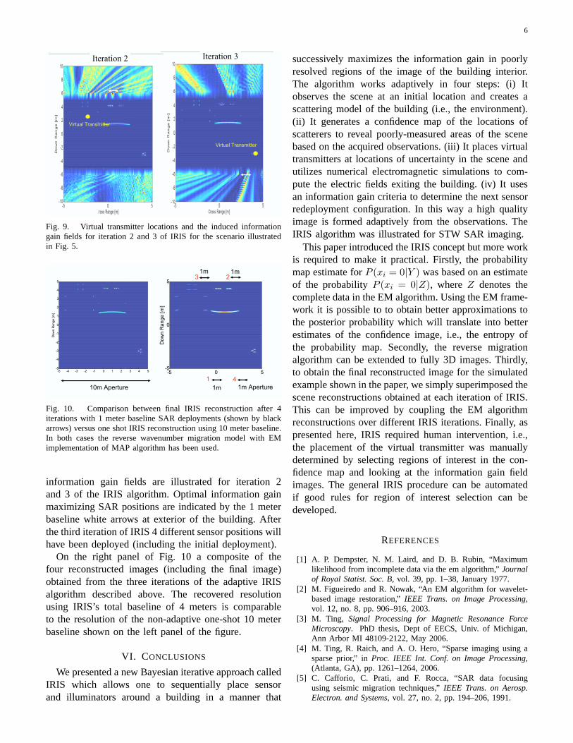
In Fig. 9 the virtual transmitter positions and induced

6

Fig. 9. Virtual transmitter locations and the induced informationgain fields for iteration 2 and 3 of IRIS for the scenario illustratedin Fig. 5.

Fig. 10. Comparison between final IRIS reconstruction after 4iterations with 1 meter baseline SAR deployments (shown by blackarrows) versus one shot IRIS reconstruction using 10 meter baseline.In both cases the reverse wavenumber migration model with EMimplementation of MAP algorithm has been used.

information gain fields are illustrated for iteration 2and 3 of the IRIS algorithm. Optimal information gainmaximizing SAR positions are indicated by the 1 meterbaseline white arrows at exterior of the building. Afterthe third iteration of IRIS 4 different sensor positions willhave been deployed (including the initial deployment).

On the right panel of Fig. 10 a composite of thefour reconstructed images (including the final image)obtained from the three iterations of the adaptive IRISalgorithm described above. The recovered resolutionusing IRIS’s total baseline of 4 meters is comparableto the resolution of the non-adaptive one-shot 10 meterbaseline shown on the left panel of the figure.

VI. CONCLUSIONS

We presented a new Bayesian iterative approach calledIRIS which allows one to sequentially place sensorand illuminators around a building in a manner that

successively maximizes the information gain in poorlyresolved regions of the image of the building interior.The algorithm works adaptively in four steps: (i) Itobserves the scene at an initial location and creates ascattering model of the building (i.e., the environment).(ii) It generates a confidence map of the locations ofscatterers to reveal poorly-measured areas of the scenebased on the acquired observations. (iii) It places virtualtransmitters at locations of uncertainty in the scene andutilizes numerical electromagnetic simulations to com-pute the electric fields exiting the building. (iv) It usesan information gain criteria to determine the next sensorredeployment configuration. In this way a high qualityimage is formed adaptively from the observations. TheIRIS algorithm was illustrated for STW SAR imaging.

This paper introduced the IRIS concept but more workis required to make it practical. Firstly, the probabilitymap estimate forP (xi = 0|Y ) was based on an estimateof the probabilityP (xi = 0|Z), whereZ denotes thecomplete data in the EM algorithm. Using the EM frame-work it is possible to to obtain better approximations tothe posterior probability which will translate into betterestimates of the confidence image, i.e., the entropy ofthe probability map. Secondly, the reverse migrationalgorithm can be extended to fully 3D images. Thirdly,to obtain the final reconstructed image for the simulatedexample shown in the paper, we simply superimposed thescene reconstructions obtained at each iteration of IRIS.This can be improved by coupling the EM algorithmreconstructions over different IRIS iterations. Finally, aspresented here, IRIS required human intervention, i.e.,the placement of the virtual transmitter was manuallydetermined by selecting regions of interest in the con-fidence map and looking at the information gain fieldimages. The general IRIS procedure can be automatedif good rules for region of interest selection can bedeveloped.

REFERENCES

[1] A. P. Dempster, N. M. Laird, and D. B. Rubin, “Maximumlikelihood from incomplete data via the em algorithm,”Journalof Royal Statist. Soc. B, vol. 39, pp. 1–38, January 1977.

[2] M. Figueiredo and R. Nowak, “An EM algorithm for wavelet-based image restoration,”IEEE Trans. on Image Processing,vol. 12, no. 8, pp. 906–916, 2003.

[3] M. Ting, Signal Processing for Magnetic Resonance ForceMicroscopy. PhD thesis, Dept of EECS, Univ. of Michigan,Ann Arbor MI 48109-2122, May 2006.

[4] M. Ting, R. Raich, and A. O. Hero, “Sparse imaging using asparse prior,” inProc. IEEE Int. Conf. on Image Processing,(Atlanta, GA), pp. 1261–1264, 2006.

[5] C. Cafforio, C. Prati, and F. Rocca, “SAR data focusingusing seismic migration techniques,”IEEE Trans. on Aerosp.Electron. and Systems, vol. 27, no. 2, pp. 194–206, 1991.

7

[6] R. Stolt, “Migration by Fourier transform,”Geophysics, vol. 43,pp. 23–48, 1978.

[7] W. Carrara, R. Goodman, and R. Majewski,Spotlight SyntheticAperture Radar. Boston: Artech House, 1995.

[8] W. Schmaedeke and K. Kastella, “Event-averaged maximumlikelihood estimation and information-based sensor manage-ment,” in Proceedings of SPIE, pp. 91–96, June 1994.

[9] K. Kastella, “Discrimination gain to optimize classification,”IEEE Transactions on Systems, Man and Cybernetics-Part A:Systems and Humans, vol. 27, pp. 112–116, January 1997.

[10] C. Kreucher, K. Kastella, and A. O. Hero, “Multi-target sensormanagement using alpha-divergence measures,” in3rd Work-shop on Information Processing for Sensor Networks, (PaloAlto, CA), pp. 209–222, 2003.

[11] J. Marble and A. O. Hero, “Phase distortion correction for see-through-the-wall radar imaging,” inProc. IEEE Int. Conf. onImage Processing, (Atlanta, GA), pp. 2333–2336, 2006.