Iterate-averaging sign algorithms for adaptive filtering with

IEEE TRANSACTIONS ON INFORMATION THEORY, VOL. 49, NO. 3, MARCH 2003 657

Iterate-Averaging Sign Algorithms for AdaptiveFiltering With Applications to Blind Multiuser

DetectionG. George Yin, Fellow, IEEE, Vikram Krishnamurthy, Senior Member, IEEE, and Cristina Ion

Abstract—Motivated by the recent developments on iterateaveraging of recursive stochastic approximation algorithms andasymptotic analysis of sign-error algorithms for adaptive filtering,this work develops two-stage sign algorithms for adaptive filtering.The proposed algorithms are based on constructions of a sequenceof estimates using large step sizes followed by iterate averaging.Our main effort is devoted to improving the performance ofthe algorithms by establishing asymptotic normality of a suit-ably scaled sequence of the estimation errors. The asymptoticcovariance is calculated and shown to be the smallest possible.Hence, the asymptotic efficiency or asymptotic optimality isobtained. Then variants of the algorithm including sign-regressorprocedures and constant-step algorithms are studied. Theminimal window width of averaging is also dealt with. Finally, it-erate-averaging algorithms for blind multiuser detection in directsequence/code-division multiple-access (DS/CDMA) systems areproposed and developed, and numerical examples are examined.

Index Terms—Adaptive filtering, asymptotic efficiency, iterateaverage, rate of convergence, sign algorithm.

I. INTRODUCTION

M OTIVATED by the ingenious procedure ofiterate aver-aging for accelerating convergence rates of stochastic

approximation algorithms, proposed independently by Polyak[28] and Ruppert [32], this work is devoted to adaptive filteringalgorithms using sign operators. We show that the convergencerates of such adaptive filtering algorithms can also be accel-erated by iterate averaging and that the resulting algorithmshave optimal convergence rates. Furthermore, we develop it-erate-averaging algorithms for blind multiuser detection in directsequence/code-division multiple-access (DS/CDMA) systemsand provide promising numerical results.

Manuscript received December 1, 2000; revised November 18, 2002.The work of G. G. Yin was supported in part by the National ScienceFoundation under Grants DMS-9877090 and DMS-9971608. The work ofV. Krishnamurthy Research was supported in part by the ARC Special ResearchCenter for Ultra-Broadband Information Networks (CUBIN), University ofMelbourne, Australia. The work of C. Ion was supported in part by theNational Science Foundation under Grant DMS-9877090 and in part byWayne State University.

G. G. Yin and C. Ion are with the Department of Mathematics, WayneState University, Detroit, MI 48202 USA (e-mail: [email protected];[email protected]).

V. Krishnamurthy is with the Department of Electrical and Computer En-gineering, University of British Columbia, Vancouver BC V6T 1Z4, Canada(e-mail: [email protected]) and the University of Melbourne, Melbourne,Australia.

Communicated by J. A. O’Sullivan, Associate Editor for Detection and Esti-mation.

Digital Object Identifier 10.1109/TIT.2002.808100

Owing to its importance and various applications in adap-tive signal processing and learning, adaptive filtering algorithmshave received much attention; see [1], [2], [9]–[12], [25], [33],[35], [37], [38], among others. Suppose that andare sequences of measured output and reference signals, respec-tively. Assuming the sequence is stationary, by ad-justing the system parameter, adaptive filtering algorithms aimto make the weighted output match the reference signalas well as possible in the sense that a cost function is minimized.If a mean square error cost

is used, the gradient of is given by

and the recursive algorithm is of the form

(1)

where as and . If the costfunction is , the gradient becomes

and a recursive algorithm takes the form

(2)

where for any ( is the in-dicator of ). Algorithm (1) is commonly referred to as a leastmean square (LMS) algorithm, whereas (2) is called a sign-erroralgorithm. Compared with (1), algorithm (2) has reduced com-plexity. Because of the use of the sign operator, the algorithmsare easily implementable and multiplications in (2) can be re-placed by simple bit shifts. As a result, it becomes appealingin various applications; see [9], [10], [12], [35] and the refer-ences therein. However, for each, as a function of ,

is not continuous. Thus, the analysis of suchan algorithm is more difficult than that of (1). Much effort hasbeen devoted to the improvement of sufficient conditions forconvergence of such algorithms. Recently, in [5], by treating analgorithm with randomly generated truncation bounds, we ob-tained that the recursive algorithm converges with probability

(w.p. ) by assuming only stationarity and finite second mo-ments of the signals, which is close to the minimal requirementneeded. In addition, we also examined rate of convergence of

0018-9448/03$17.00 © 2003 IEEE

658 IEEE TRANSACTIONS ON INFORMATION THEORY, VOL. 49, NO. 3, MARCH 2003

the algorithm by weak convergence methods. A crucial obser-vation is that although the functions are not continuousin , can be a smooth function thanks to the smoothingeffect provided by taking expectation. Note that Gaussian ap-proximation and central limit results for adaptive signal processalgorithms have also been considered, for example, in [2], [33]among others. Notably, Markovian-type processes are treated in[2] and stochastic averaging ideas are used in [33].

In this paper, in addition to (1) and (2), an algorithm knownas a sign-regressor algorithm used frequently in applications,will also be considered. In this case, in lieu of (2), one usessign operator only for the regressor by taking the signof componentwise. Experience with numerical examplesshows that the sign-regressor algorithm often outperforms (2).The rationale for using sign-regressor algorithms is to takeadvantages of both LMS and sign-error algorithms and to havethe performance close to that of (1) with less complexity. De-voted to (2) and its variations such as sign-regressor algorithmsand algorithms with constant step size, in comparison to therecent study on the sign-error algorithms, we shift gear andemphasize the asymptotic efficiency issues. Our plan is asfollows. We first develop the iterate-averaging sign-error al-gorithms. Then we proceed with the analysis of sign-regressoralgorithms without providing verbatim proofs since they canbe carried out similarly to those of sign-error algorithms withweaker conditions and simpler proofs. An alternative methodfor analyzing the averaging algorithms is along the line ofstrong approximation. We refer the reader to [26], [27] forrelated references and further study.

Inspired by the recent work on iterate averaging of stochasticapproximation algorithms [28], [32], [21], we propose severaliterate-averaging algorithms for sign adaptive filtering algo-rithms. The motivation behind the averaging approach can betraced back to the work of Chung [7] and many subsequentpapers on adaptive stochastic approximation. Nevertheless, ithas been shown that the iterate-averaging approach leads toasymptotic optimality (the best scaling factor and the minimalvariance) and has advantages for various applications. First, itsinitial approximation uses slowly varying step sizes larger than

to get rough estimates, which enables the iterates toget to a neighborhood of the minimizer faster than that ofa small step-size procedure. Then, by averaging the iterates,the resulting sample path possesses the minimal variance. Oureffort in what follows is to prove that the iterate-averagingadaptive filtering algorithms are asymptotically optimal.

The rest of the paper is arranged as follows. Section II isdevoted to the iterate-averaging of sign-error algorithm. Itprovides the convergence of algorithm (2) and obtains theconvergence of . The asymptotic efficiency issue is thenstudied. Section III proceeds with the ramifications and vari-ations of the iterate-averaging approach. We study averagingin sign-regressor algorithms, algorithms with constant stepsize, and minimal window width of averaging. To demon-strate the performance of the algorithms, a case study ofblind interference suppression in DS/CDMA spread-spectrumtelecommunication systems is provided in Section IV. Sec-tion V gives further remarks. Finally, an appendix containingthe proofs of some technical results, concludes the paper.

Throughout the paper, we use to denote the transpose offor , , and use to denote the norm of.

For notational simplicity, denotes a generic positive constantwhose values may vary for different usage. For a square matrix

, by we mean that it is positive definite.

II. I TERATE-AVERAGING SIGN-ERRORALGORITHMS

A. Convergence of Sign-Error Algorithm

Consider the two-stage sign-error algorithm

(3)

In what follows, we use to denote the conditional ex-pectation with respect to , the -algebra generated by

. Define

and

To proceed, we state the conditions needed.

has a unique minimizer, denoted by .is a stationary sequence with

For each , is continuous; there is ansuch that for each

w.p.

and (4)

where is Hurwitz, i.e., all of its eigenvalues havenegative real parts. Either is a martin-gale difference sequence satisfying ,

for some , or it is a boundeduniformly mixing sequence such that there is a deter-ministic sequence of real numbers satisfying

for each , , and for eachand some

and

(5)

Remark 2.1:We have collected the conditions needed forboth convergence and rate of convergence in (A). As far as con-vergence alone is concerned, not all aspects of the assumptionsare needed.

By (4), is locally (near ) linearizable. To seethis, suppose that the joint density of and exists.Denote by the conditional distribution with respectto and by the correspondingconditional density. It can be seen that

YIN et al.: ITERATE-AVERAGING SIGN ALGORITHMS FOR ADAPTIVE FILTERING 659

Moreover, for any , the partial derivatives of exist. Usingto denote theth component of , and using and

to denote the th components of and , respectively, wehave

see also [12, p. 195] and [5]. Thus, a sufficient condition for(4) is that is differentiable with bounded derivatives.Moreover, if and are independent and identicallydistributed (i.i.d.) random variables or martingale difference se-quences, where is thedensity of .

Condition (5) requires the signals andhaving decreasing dependence as .

The is referred to as a uniform mixing measure in [8, p.348]; see also [3, p. 200]. The inequality is reminiscent of thewell-known mixing inequalities (see [3], [8], [19]).

The noise sequences covered by the conditions includebounded and uniform mixing sequences, or uncorrelatedsignals with finite th moment, or combination of them.Note that for uncorrelated signals, (5) is trivially satisfiedand the conditional expectation is replaced by expectation.The conditions for an moving average process oforder driven by a martingale difference noise are similar tothose of the martingale difference noise; we need only placethe conditions on the driving noise instead of on and(The analysis can be carried out as in [38].) If the sequence

is bounded and uniform mixing with mixing rate(see [19, p. 82] and [8, p. 349]), then so are and

. By the stationarity, , and itfollows from (5) that if

and

(6)

Note that the bounded mixing signal is not restrictive. Inpractice, one often wants to avoid excessively large valuesof the observation. Although modeling at large values oftenfollows from traditional setup (such as Gaussian assumptions),it is undesirable for single observation to have significant effecton the iterations. Thus, one often uses a robust algorithm. Forthe sign-error algorithm that we are interested in, we can use

(7)

where for a vector suchthat for , are bounded real-valued functions on thereal line that are nondecreasing and that satisfy ,

, and as . Forfurther discussions on the use of such functions and robust algo-rithms, see [29] (also [22, Sec. 1.3.4, p. 22]). For the sign-erroralgorithm, due to the boundedness of , the use of

the function is equivalent to the truncation of . However,for notational simplicity, we choose to use the bounded mixingcondition here. Moreover, an alternative procedure projects theiterates into a bounded region (e.g., a hyperrectangle); see [22]for more discussion.

Theorem 2.2:Assume (A) and is the global asymptoticstable point of the ordinary differential equation (ODE)

, where is an average of . Then w.p. ,and w.p. .

Remark 2.3: In lieu of an algorithm with expanding randomtruncation bounds as in [5], we examine the algorithms directly.Using the treatment of stochastic approximation algorithms of[22], the proof of convergence is converted to the verification ofa recurrence condition by using [22, Theorem 7.1, p. 163]. Infact, we need only verify that the recurrence condition, namely,“for each , let there be a compact set such that

infinitely often (i.o.) with probability at least” is ver-ified, then as in the argument of [22, p. 164],w.p. . As a result, using the ODE method, a sequence of piece-wise-constant interpolation of the iterates is uniformlybounded and equicontinuous in the extended sense (see [22, p.73]). for a definition). By virtue of the Ascoli–Arzelá theorem,we obtain that any convergent subsequence has a limitsat-isfying . A stability argument then impliesw.p. . Therefore, only the recurrence needs to be verified. By[22, Theorem 7.2, p. 164], a sufficient condition that guaranteesthe recurrence is: is bounded in probability. That is, forany , there is a such that .Since by Chebyshev’s inequality

which can be made if , and (or), which can be established via a Liapunov function

argument. Since we will prove a result with a sharper bound onin Theorem 2.4 using similar techniques, we omit the

details here.

B. Asymptotic Efficiency

This subsection is devoted to the asymptotic efficiency of thesign algorithm. As was mentioned, the heart of the problem isto show that is asymptotically normal with theoptimal covariance matrix. In fact, we obtain a more interestingfunctional invariance theorem.

Define and . Then (3) can be rewrittenas

(8)

The proof of the following bounds via Liapunov theory is in-cluded in the Appendix.

Theorem 2.4:Under (A), for sufficiently large ,, and the bounds hold uniform in.

Much effort has been devoted to improving the rate of con-vergence and to reduce the asymptotic variance in the adap-tive estimation problems. Consider (2) with ,

. Under suitable conditions, it can be shown that


converges in distribution to a normal randomvariable as . It is clear that among the pos-sible ’s with , gives us the best scalingfactor. Since in evaluating rates of convergence, one uses thescaling factor together with the asymptotic covariance matrix

, for different algorithms with , we wish to findthe one with minimal variance. The idea outlined in [7] is toconsider (2) with , where is a (matrix-valued) pa-rameter. It follows that the asymptotic covarianceis a smooth function of . Minimizing with respect to(w.r.t.) leads to the choice and the optimalvariance , where is the noise co-variance and is defined in (4). Although is explicitlygiven, is virtually unknown. To circumvent such a diffi-culty, researchers developed step-size-adaptation algorithms. Inthe context of adaptive filtering, this amounts to constructinganother sequence , estimates of , on top of the adap-tive filtering estimate. Then use a sequence of matrix-valuedstep-size in the actual estimation, denoted by. Itcan be shown that such a recursive least squares (RLS) type al-gorithm is convergent and . Althoughoptimality is obtained, the RLS algorithm has computationalcomplexity compared to the order complexity of ascalar step size stochastic approximation algorithm. A new ap-proach, initiated in the late 1980s [28], provides a much betteralternative (see also a scalar version of the algorithm in [32]).Instead of adaptively generating the matrix-valued estimates, asimple iterate-averaging approach is used leading to the desiredasymptotic optimality. The corresponding problems for adap-tive filtering under quadratic cost functions were treated in [38]among others. We will show that the averaging approach forthe sign algorithms of adaptive filtering also leads to asymptoticoptimality. Rather than dealing with the iterates as in [38], wework with suitably interpolated sequences. As a preparation, wefirst derive an asymptotic equivalence. Then we proceed with aninvariance theorem. In order not to disrupt the flow of presenta-tion, we relegate their proofs to the Appendix.

Using (A) and

rewrite the first equation in (3) as follows:

(9)

where is defined in (4) and

(10)

Note that and hence is a martingale dif-ference sequence. Define

if

if

It follows from (9) that for any integer and

(11)

Next, consider a continuous-time interpolation

for (12)

where denotes the integer part of. Then we have

where

Since is nonsingular

and

Thus, for each

where

(13)

Lemma 2.5:The following estimates hold:

for each and

as (14)


The proof of the lemma is in the Appendix. To proceed,choose such that

but as (15)

We further derive the following lemma; its proof is in theAppendix.

Lemma 2.6:

as , where in probability uniformly in .

We proceed to obtain a functional central limit theorem orinvariance theorem. The proof is standard; see, for example, [3],[8], [22]. In fact, under (A)

converges weakly to a Brownian motion

(16)with covariance , where

(17)

The proof of the following theorem is also in the Appendix.

Theorem 2.7:Under (A), defined in (12) is tightin , and it converges weakly to a Brownian motion withcovariance , where with and

defined by (4) and (17), respectively.

III. I TERATE-AVERAGING SIGN-REGRESSORALGORITHMS

A. Sign-Regressor Algorithm With Iterate Averaging

In lieu of (2), by taking sign componentwise, we obtain theso-called sign-regressor algorithm. In this section, we consideran iterate-averaging sign-regressor algorithm

(18)

where denotes for. To carry out the asymptotic analysis, we need the fol-

lowing conditions.

is stationary with ,and , where is Hurwitz. Either

is a martingale difference sequence satis-fying , for some ,or it is bounded and uniformly mixing with mixing rate

satisfying .

Remark 3.1: It is easily seen that the conditions are muchweaker than (A) used before. The sequence is sta-tionary, so are , , and .Moreover, is bounded by w.p. . Since we onlytake the sign of componentwise, the nonsmoothness of

in the sign-error algorithm (3) is removed. As a result, the anal-ysis is simpler. In addition, conditions for an processdriven by a martingale difference noise can also be provided(see Remark 2.1).

Proceeding as in Section II, under (B), we can verify therecurrence condition, and show that defined in (18) con-verges w.p. . Define , take a continuous-timeinterpolation of the iterates , for

, , and let be the unique suchthat . Using the ODE methods [22, Chs. 5 and 6],we can show that is uniformly bounded and equicon-tinuous in the extended sense. Then the Ascoli–Arzelà theoremimplies that any convergent subsequence has a limitsatis-fying the limit ODE

(19)

with the unique stationary point . Moreover, (B)implies that (19) is asymptotically stable. We then obtain thefollowing result.

Theorem 3.2:Under condition (B), defined by (18)converges w.p. to .

Remark 3.3: It is interesting to compare (18) with thealgorithm (1). Under stationarity of the signals and assuming

, the limit of the ODE for (1) and the uniqueminimizer of the quadratic cost functions are

(20)

respectively. They are similar to that of (19). As a result, the twoalgorithms have similar asymptotic behavior. The difference isthat is symmetric, whereas in (18), the symmetry is lost.We only assume the eigenvalues of have positivereal parts. To some extent, the sign-regressor algorithm is one“between” the LMS algorithm and the sign-error algorithm. Asa result, its performance is close to LMS algorithm and its com-plexity is similar to the sign-error algorithm.

To proceed, define

Denoting as before, we have

Define

if

if .

Similar to (11), we arrive at for any

(21)

Next define

for , where is given by (18). Similarly as in Sec-tion II, we obtain the following.


Theorem 3.4:Under (B), converges weakly to aBrownian motion whose covariance is

where is given in condition (B) and

(22)

B. Minimal Window of Averaging

So far, we have only considered the averaging with windowwidth . In [21], averaging with “minimal” window width,the smallest window width needed to be effective for improvingthe performance, was considered. From an application point ofview, the minimal window of averaging provides a useful in-sight. Following the approach outlined in [22, Ch. 11.1], let usillustrate the idea by use of the sign-regressor algorithm. For it-erates given by (18), for and

, define

(23)

Taking the averaging window width to be rather thanas before, for any , define

(24)

It follows that

where in probability uniformly in . Using the weakconvergence method (see [22, Chs. 8 and 10]), we establish that

converges weakly to , which is the stationary solutionto

(25)

where is the “square root” of given in (22). By in-voking [22, Theorem 1.1, p. 331], we obtain the following.

Theorem 3.5:Assume (B). For each , treatas a sequence of random variables. Then converges indistribution to a normal random vector with mean andcovariance where is defined inTheorem 3.4.

C. Constant-Step-Size Algorithms

In many practical applications of adaptive filtering such asthe interference suppression example discussed in Section IV,

constant-step-size algorithms are required for tracking slowlyvarying parameter variations. This subsection considers iterateaveraging for theconstant step sizesign-regressor algorithm.The algorithm is

(26)

where denotes a forgetting factor applied to theaveraging procedure. Since the minimal window of averagingis of particular importance, the following discussion is devotedto such cases.

Case i): Decreasing Forgetting Factor :Using (B) and for definiteness, let us concentrate on the caseof bounded mixing condition. Then [3, p. 197] and [8, Ch. 7.3]imply that converges weakly to a Brownianmotion with covariance , where is given by (22). Thesequence is uniform mixing, so areand . Therefore, they are strongly ergodic. Con-sequently, for any

(27)both in probability. (In fact, they converge w.p., but forour analysis, convergence in probability is sufficient.) Define

for . Similar to [20], we obtainthe following. Assume converges to and (B). Thenconverges weakly to , which is a solution to the differentialequation (19). Furthermore, for any as ,

converges weakly to given by (19).Define and for .

Then it can be shown that converges weakly to ,a solution of (25), as and . To proceed, define

Using the argument of [22, p. 333], we obtain the following.

Theorem 3.6:Assume converges to and (B). Then, foreach fixed , converges in distribution to a normalrandom vector with mean , covariance ,and defined in Theorem 3.4.

Case ii): Constant Forgetting Factor: Here we take a con-stant forgetting factor with . In the analysis,we examine the asymptotic properties of the dynamic systemgiven by (26) as and , whereas in the imple-mentation, and are kept as constants. Define

(28)

By using the interpolations and , a similar argumentas in Theorem 3.6 leads to the following result.

Theorem 3.7:Assume (B). For each fixed , con-verges in distribution to a normal random vector with mean, covariance , and defined in Theorem 3.4.


D. Remarks on AveragedSign-Error and LMS Algorithms

The discussions thus far readily carry over to minimal win-dows of averaging for the following decreasing step-size andconstant step-size sign-error algorithms:

(29)

where . Moreover, either a constant forgettingfactor or a sequence of decreasing forgetting factors can beincluded. Results similar to Theorems 3.5, 3.6, and 3.7 can beobtained with the use of condition (A) in lieu of (B) and with

replaced by given in Theorem 2.7.Similar results for minimal windows for averaging and con-

stant step size LMS algorithms with averaging can be estab-lished by using the techniques of [22]; we summarize the resultsas follows. For fixed , , as defined in (28), converges indistribution to a normal random variable with meanandcovariance , where

(30)

and

(31)

IV. CASE STUDY: SIGN ALGORITHMS FORBLIND MULTIUSER

DETECTION IN DS/CDMA SYSTEMS

DS/CDMA is among the most promising multiplexingtechnologies for cellular telecommunications services suchas personal communications, mobile telephony, and indoorwireless networks. Demodulating a given user in a DS/CDMAnetwork requires processing the received signal to minimizetwo types of interference, namely, narrow-band interference(NBI) and wide-band multiple-access interference (MAI)caused by other spread-spectrum users in the channel—as wellas ambient channel noise [15]. NBI is caused by the coexistenceof spread-spectrum signals with conventional communications;see [15] and [17] for a recent review of active NBI suppressionmethods that have resulted in substantial gains in DS/CDMAsystems. MAI arises in DS/CDMA systems due to the fact thatall users communicate through the same physical channel usingnonorthogonalmultiplexing, which has many advantages inwireless CDMA systems such as greater bandwidth utilizationunder conditions of channel fading and bursty traffic.

Recently,blind multiuser detectiontechniques [14], [30], [31]have been developed that allow one to use a linear multiuser de-tector for a given user with no knowledge beyond that requiredfor implementation of the conventional detector for that user.Blind multiuser detection is useful in mobile wireless channelswhen the desired user can experience a deep fade or if a stronginterferer suddenly appears. In [14] a blind LMS algorithm isgiven for linear minimum mean-square error (MMSE) detec-tion. In [31], a code-aided blind RLS algorithm for jointly sup-pressing MAI and NBI is given. More recently, in [16], a blindaveraged LMS algorithm is presented with a heuristic mean-

square error convergence analysis in the same spirit as [14] and[31].

The objective of this section is to use the averaged sign-errorLMS and the sign-regressor LMS algorithms analyzed in Sec-tions II and III of this paper to the MMSE detection scheme formultiuser detection in a DS/CDMA system. The performanceof the sign algorithms will be studied and compared with that ofthe standard LMS.

A. DS/CDMA Signal Model

Consider a synchronous-user binary DS/CDMA commu-nication system. Assume that this system transmits throughan additive white Gaussian noise channel. After the receivedcontinuous-time signal is preprocessed and sampled at theCDMA receiver (the received signal is passed through achip-matched filter followed by a chip-rate sampler), theresulting discrete-time received signal at time, denoted by

, is given by (see [31] for details)

(32)

Here is an -dimensional vector; is called the processing(spreading) gain; is an -vector denoting the normalizedsignature sequence of theth user, i.e., each element

for , so that ;denotes the data bit of theth user transmitted at time;

is the received power of theth user; is the NBIsignal -vector, which is assumed to be a bounded stationaryautoregressive (AR) process with mean zero and covariance ma-trix ; is the standard deviation of the noise samples;isa white Gaussian vector with mean zero and covariance matrix, where denotes the identity matrix. It is assumed that

the discrete-time stochastic processes , , andare mutually independent, and that is a collection of in-dependent equiprobable1 random variables.

We assume that user 1 is the user of interest. Following thedefinition of , denotes the normalized signature sequenceof user 1. For user 1, the term in (32) istermed MAI. The aim of a multiuser detector is to suppressthe MAI and adaptively estimate (demodulate) the bit sequence

given the observation sequence. A linear blind mul-tiuser detector demodulates the bits of user 1 according to (see[31] for details) , where denotes theestimate of the transmitted bit at time , and denotes anappropriately chosen “weight vector.” In this section, we focuson the widely used code-aided blind linear mean output error(MOE) detector [14], [31] which chooses the “weight vector”so as to minimize the MOE cost function

subject to (33)

The constraint ensures that the received energy from the user ofinterest is equal to 1. Thus, the above is a minimization of theenergy from the interferers. Furthermore, as shown in [14], theMOE cost function has a unique global minimum (with respectto ). The blind MOE detector yields the following estimate

of the transmitted signal (see [31] for details):

where (34)


and denotes the autocorrelation matrix of the re-ceived signal . In the preceding equation, is the optimallinear MOE “weight vector.” Such a detector is “blind” sinceit does not assume any knowledge of the data symbolsand signature sequences of other users.

The output signal-to-interference ratio (SIR) is widely usedto characterize the performance of a linear multiuser receiver.The SIR for an arbitrary weight vectoris defined as

SIR (35)

The SIR of the optimal weight vector and the MOE of aregiven by [31, eqs. 5 and 7, respectively]

SIR

(36)

B. Adaptive Sign Algorithms for Blind Multiuser Detection

In adaptive blind multiuser detection problems, we areinterested in recursively adapting the weight vector tominimize , the MOE given by (33). In particular, it is oftennecessary to use a constant step-size tracking algorithm dueto the time-varying nature of caused by the birth and deathof users (MAI interferers). We now present constant step-sizeversions of the sign-regressor and sign-error algorithms forblind adaptive multiuser detection.

In presenting the sign algorithms for blind adaptive multiuserdetection, it is convenient to work with an unconstrained opti-mization problem rather than (33). Let , fordenote the components of . The constrained optimizationproblem (33) may be transformed into an unconstrainedoptimization problem by solving for one of the elements ,

using the constraint (33). With no loss ofgenerality, we solve for the first element and obtain

By defining the -dimensional vector

we obtain the equivalent unconstrained optimization problem

Compute where (37)

Here, and denotes the -dimen-sional vector

As in (20), let denote the MMSE solution

It is straightforward but tedious to show that the componentsof are indeed the last elements of optimal weightvector defined in (34). Using the defined above, we callthe constant step-size sign-regressor algorithm (26) with fixedforgetting factor operating on the DS/CDMA signal model(32) as theblind averagedsign-regressor algorithm. Similarly,

we call the constant step-size sign-error algorithm (29) as theblind averagedsign-error algorithm.

Remark 4.1:When is small, computations using andmay become ill-conditioned. This is trivially taken care of as

follows. because , in and .

Canonical Coordinates. In [14], constraint (33) for theblind LMS algorithm is taken care of by introducing canonicalcoordinates together with a MSE analysis. The essential ideais to replace the unconstrained gradient of the MOE in (33),namely, , by its component orthogonal to , namely,

. The blind averaged LMS and blind av-eraged sign-error algorithm can be expressed in canonicalcoordinates as

respectively. It is easily seen that the estimatesin the abovetwo algorithms automatically satisfy constraint (33). However,it is not possible to derive a sign-regressor algorithm in canon-ical coordinates that satisfies constraint (33). For example, thesign-regressor algorithm in canonical coordinates

doesnot satisfy constraint (33). In the numerical examplespresented later, we found the performance of the blind averagedLMS and sign-error algorithms in canonical coordinates areidentical to the corresponding algorithms derived for the uncon-strained cost function. However, it is more convenient to workwith the equivalent algorithm derived for the unconstrainedcost function.

C. Performance Analysis of AveragedAlgorithms

Note that we have assumed that is a bounded sequenceof regressive process (e.g., stationary truncated Gaussian au-toregreesive process), and that and are i.i.d. pro-cesses. It follows that is a sum of bounded mixing sequenceand martingale difference sequence, so the noise condition in(A) is satisfied. Thus, all the convergence and asymptotic opti-mality results derived in Sections III-C and -D for the averagedsign-error and sign-regressor algorithms hold. To proceed, wederive approximate expressions for , , and andthe asymptotic excess mean-square error and SIR of the aver-aged and un-averaged sign LMS algorithms for the DS/CDMAsignal model. These are commonly used performance measuresfor adaptive filtering algorithms in the signal processing andCDMA literature; see [14] or [31]. In what follows, we useand , the covariance matrices defined in condition (B) and(31).

To obtain expressions for the asymptotic excess mean-squareerror, we first note that the zero mean estimation errorof theMMSE (Wiener) solution , given by

(38)

is uncorrelated with —this is the principle of orthogonality[13] for the MMSE solution , which is easily verified. Note


that for the DS/CDMA signal model (32), using (36), and thedefinition of the equivalent unconstrained problem (37), wehave .

We need the following additional assumptions:

i) and are independent.

ii) The input data and the previous weight vector arestatistically independent [13, Ch. 9].

These two assumptions are not needed for the weak convergenceanalysis presented earlier. They are introduced only to give sim-plified closed-form expressions for the weighted error correla-tion, excess mean square error, and steady-state SIR. Withoutthese assumptions, the expressions would involve fourth-ordermoments—while these can be computed, the resulting expres-sions are messy and yield little insight (see also [14]).

Assumption i) is justified when for fixed processing gain,the number of users is large. Assuming the binary signaturesequences are chosen randomly (equiprobably over all choices)and the amplitudes are identical, one can apply the i.i.d.version of the central limit theorem to (32). Alternatively, if theamplitudes , , the Lindberg–Fellercentral limit theorem, see [36, pg. 150], can be applied. Thecentral limit theorem implies is asymptotically a zero-mean

-dimensional Gaussian random vector. This in turn impliesis approximately an -dimensional zero-mean

Gaussian random vector, andand are scalar zero-meanGaussian random variables. Since orthogonality for Gaussianrandom variables is equivalent to independence,and areasymptotically independent.

Note that assumption ii) is satisfied if the interference con-sists only of MAI and white noise. This assumption is used in[31] for analyzing the blind RLS algorithm; it is also commonlyused in deriving closed-form expressions for the performanceof adaptive filtering algorithms (see [13]).

Weighted Error Correlation : The weighted error corre-lation matrices for the various averaged algorithms can beobtained from the analysis of Sections IV-A and –B as follows.

. Consider given in (30).Because of i) and ii) above, in (31) can be computed as

Let denote the weighted error correlation ma-trix. Note that is an positive-definitematrix. Then (30) implies that

(39)

. Considergiven in Theorem 3.4. Using results i) and ii), in (22) is

since . We have theweighted error correlation matrix

(40)

Next, as in [10], we use assumption ii) above which implies thatis approximately a Gaussian sequence. Then Price’s formula

yields

where

(41)

. With defined inTheorem 2.7, using results i) and ii) above, in (17) is givenby

Thus, the weighted error correlation matrix satisfies

(42)

Under the Gaussian assumption, [6, eq. (39)] shows thatwhere .

Asymptotic Excess Mean Square Error:The MOE de-fined in (33) can be expressed again as

Since as , the last term is asymptoticallyunimportant. Hence, for large, where theexcess mean square error is defined as

(43)

In what follows, we compute expressions for the asymptotic ex-cess mean square error .

. It follows from (39) that

(44)

Note that the above equation is identical to that of the blindRLS, see [31, eq. 40]. As for blind RLS, the steady-state misad-justment of the averaged LMS algorithm is independent of theeigenvalue distribution of the data autocorrelation matrix.

. Using the Gauss-ian assumption which implies (41) together with (40) and (43)yields

(45)

We can easily compute a lower bound for by boundingin terms of as follows. Let ,, be the eigenvalues of the positive-definite sym-

metric matrix . Since all the diagonal elements ofthis matrix are


TABLE IASYMPTOTIC EXCESSMEAN SQUARE ERRORS� (1)

lower bound

Using the well-known inequality that the harmonic mean is lessthan the arithmetic mean, we obtain

which implies that

and

. It follows from (42)that

(46)

Just like the blind RLS algorithm and the blind averaged LMSalgorithm analyzed earalier, the steady-state misadjustment ofthe averaged sign-error algorithm is independent of the eigen-value distribution of the data autocorrelation matrix.

It is illustrative to compare the asymptotic excess mean-square error of the averaged sign algorithms with their standard(unaveraged) counterparts. Expressions for the asymptoticexcess mean-square error of the standard sign-error algorithmshave been derived in [6] and for the sign-regressor algorithm in[10]. Table I summarizes the results.

Remark 4.2: i) All the expressions for the standard algo-rithms above assume that . In particular, terms involving

are negligible. More precise expressions are available in [6]and [10]. The expressions for the sign-regressor algorithm givenare lower bounds. ii) for the averaged algorithms donot depend on the eigendistribution of . This is particularlyuseful in dynamic mobile environments where the eigenstruc-ture of can change rapidly. In [31], a similar propertyis shown for the blind RLS algorithm. It only remains to givetractable expressions for . It is tedious but straightfor-ward to show that

SIR: The SIR Defined in (35) can be reformulated in terms ofthe asymptotic excess mean-square error as

SIR SIR SIR

D. Numerical Examples

In this section, computer simulations are presented that il-lustrate the performance of the averaged sign algorithms. Fora detailed numerical study of the averaged LMS algorithm inblind-multiuser detection, please refer to [16]. As is common in

the CDMA literature, we use the steady-state SIR as the figure ofmerit for assessing the interference suppression capability of thevarious algorithms. All the signal and noise powers are given indB relative to the channel noise variance, see (32). The sim-ulations below assume a synchronous DS/CDMA system withprocessing gain . The desired user’s signature is gen-erated as an -sequence. The signature sequences of the otherMAI’s are generated randomly.

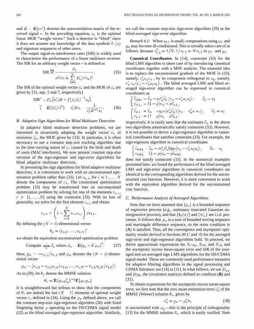
Example 1 (MAI Suppression):The user of interest has SNRof 20 dB. There are 7 multiple access interferers: 5 users eachof SNR 20 dB, and two users of SNR 40 dB. Fig. 1 shows theSIR versus time for the following six algorithms, averaged over100 independent simulations: a) blind LMS versus blind aver-aged LMS; b) blind sign regressor versus blind averaged signregressor; c) blind sign error versus blind averaged sign error.

In addition, we also simulated the blind RLS algorithm givenin [31]. The blind RLS algorithm and averaged blind LMS al-gorithm yielded virtually indistinguishable SIR plots. It is seenfrom Fig. 1 that the averaged LMS and averaged sign algorithmsexhibit faster convergence than the unaveraged algorithms.

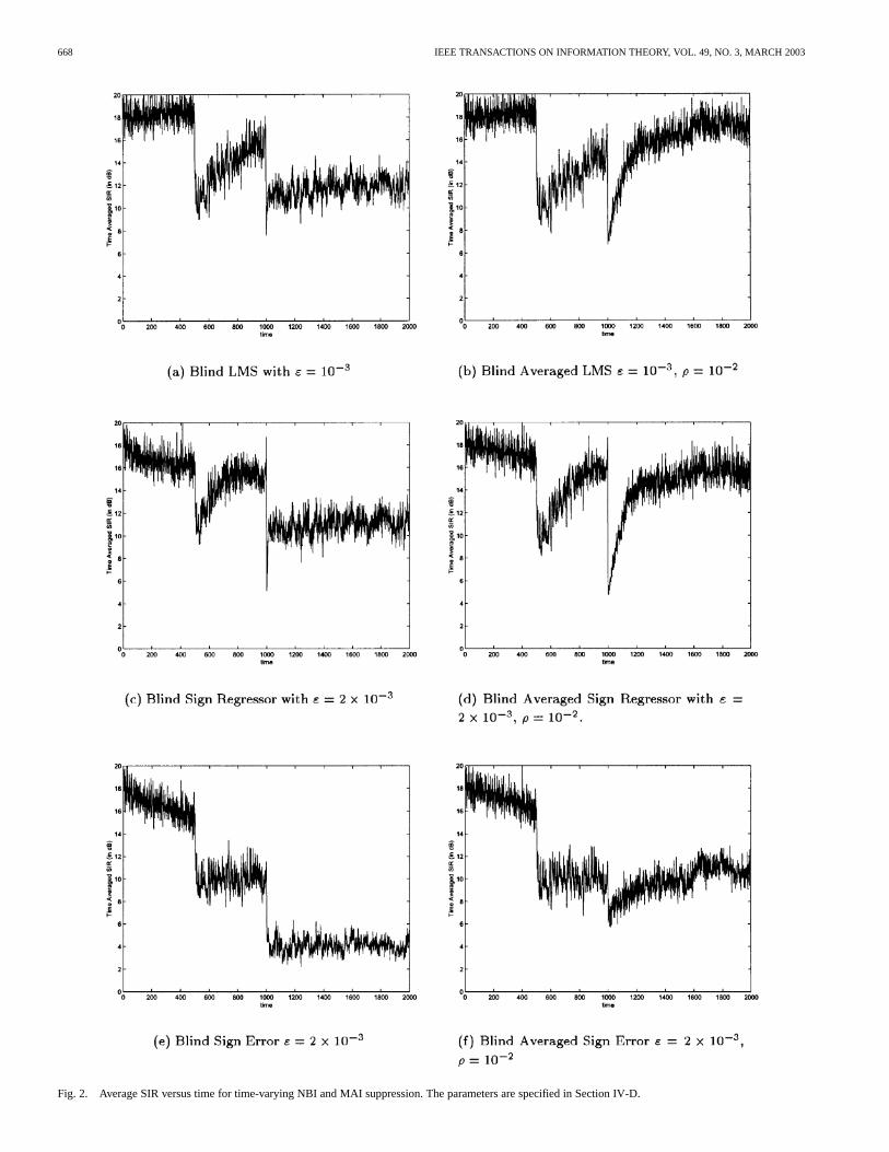
Example 2(Dynamic Environment—MAI and NBI WithTime-Varying Statistics):The simulation starts with onedesired user’s signal and 6 MAI signals each of 20 dB. Attime 500, a 10-dB NBI interferer is added to the system. TheNBI signal is a bounded stationary AR signal with both polesat 0.99. At time 1000, another strong MAI signal of 40 dB isadded. At time 1500, three of the original 20-dB MAI signalsare removed from the system. Fig. 2 shows SIR versus time forthe six algorithms averaged over 100 independent simulations:

a) blind LMS with step size ;

b) blind averaged LMS with , ;

c) blind sign regressor with (for imple-mentation using binary shifts);

d) blind averaged sign regressor with ;.

e) blind sign error with ;

f) blind averaged sign error with ,.

It is seen that in all cases, the averaged algorithms have betterconvergence properties than the algorithms without averaging.Also, it is interesting to note that the sign-regressor algorithmperforms similarly to the LMS algorithm whereas the sign-erroralgorithm performs worse.

V. FURTHER REMARKS

Iterate-averaging algorithms have been developed in thispaper, and have been shown to be asymptotically efficient in thesense that , where (with ,or , or depending on the type of algorithms) is theoptimal asymptotic covariance. In fact, a functional centrallimit theorem is obtained and the usual central limit theorembecomes a corollary. As pointed out in [38], the asymptoticoptimality cannot be improved by placing a constant in the


Fig. 1. Average SIR versus time for MAI suppression. The parameters arespecified in Section IV-D.

gain. That is, if we replace by for some constant,the will not show up in the asymptotic covariance.

Using essentially the same analysis but with more complexnotation, we can obtain similar results with more general stepsize in lieu of the slowly varying step size usedin this paper. For some of the related references, we refer thereader to [22, Ch. 11].

In a recent work [18], we have applied the sign algorithm todiscrete stochastic approximation for optimization of spreadingcodes. For future study, one may consider further properties ofsuch algorithms. In addition, one may consider an averagingalgorithm with feedback; see [22, p. 60] and the referencestherein. One may also study algorithms using averaging in bothiterates and observations. Another interesting problem is toconsider the associated adaptive step-size algorithms (see [2]and [22, p. 53]).

APPENDIX

A. Proof of Theorem 2.4

We use the techniques of perturbed test function to obtain theestimate. Define . Note that is -measur-able so is . By virtue of condition (A), for sufficiently large ,

(47)

To proceed, we introduce the perturbations and define

(48)

By virtue of (5)

and

(49)

so the perturbations are small. We show that they also lead todesired cancellations. Direct computation yields that

(50)

Similarly, we obtain

(51)


Fig. 2. Average SIR versus time for time-varying NBI and MAI suppression. The parameters are specified in Section IV-D.


The Hurwitz assumption on implies that there is asuch that for some . It follows thatthere is a with such that

(52)

Using (47)–(52)

It follows from (49) that for some

(53)

Taking expectation in (53) and iterating on the resultinginequality

Moreover, by using (49), we also have .Furthermore, the bounds derived are uniform in. This con-cludes the proof.

B. Proof of Lemma 2.5

Using telescoping

(54)

Since is stable, there is a such that

for

Thus, is bounded yielding the first inequality in(14). The second equation in (14) is proved in [4, p. 9].

The following proofs are carried out by using bounded mixingconditions. The proofs under martingale difference signals or

processes are much simpler.

C. Proof of Lemma 2.6

1) We first show that under (A) and (15),in probability as uniformly in . Since

is bounded w.p. (Theorem 2.2), w.p. by (15). By(13)

Since

by Theorem 2.4, and , inprobability.

Using and interchanging the orders ofsummations, we obtain

by (13) and (14).2) We show that for , , and

where , , , andin probability uniformly in . In fact, using the

Dirichlet formula to interchange the order of summations in, , and , we obtain

Note that by virtue of (13), for

(55)

First, we have that as

(56)


by virtue of the mixing property of , and by Lemma 2.5.For the corresponding term in , since is a martin-

gale difference sequence, it is uncorrelated and by Lemma 2.5,as

(57)

Finally, we come to the terms in . By using Theorem 2.4,. This together with Lemma 2.5 and the

boundedness of the signals yields that as

(58)

Combining (56)–(58), the desired result follows.3) We next show that and contribute nothing to

the limit, so only is asymptotically important. To provein probability uniformly in , it suffices to consider

in accordance with step 2)above. First, note (59) at the bottom of the page. By using themixing inequality (6), we have

as

Moreover

as

The above estimates and (59) then lead to that as.

Finally, for , since is a martingale differencesequence

(60)

Note that as , that as, that , and that is

continuous in by condition (A). Note also that as a function of, is bounded and is dominated

by a linear function of . In view of (10), the dominatedconvergence theorem and as yieldthat the last term in (60) goes touniformly in .

D. Proof of Theorem 2.7

By virtue of Lemma 2.6, and the choice of ,

as , where in probability. Thus, isalso tight in . Moreover, (16) and Slutsky’s theoremyield the desired result.

(59)


ACKNOWLEDGMENT

The authors are grateful to the referees and the Associate Ed-itor. They thank them for the detailed comments, suggestions,and corrections on an early version of the manuscript.

REFERENCES

[1] A. Benveniste, M. Gooursat, and G. Ruget, “Analysis of stochastic ap-proximation schemes with discontinuous and dependent forcing termswith applications to data communication algorithms,”IEEE Trans. Au-tomat. Contr., vol. AC-25, pp. 1042–1058, Dec. 1980.

[2] A. Benveniste, M. Metivier, and P. Priouret,Adaptive Algorithms andStochastic Approximations. Berlin, Germany: Springer-Verlag, 1990.

[3] P. Billingsley, Convergence of Probability Measures, 2nd ed. NewYork: Wiley, 1999.

[4] H. F. Chen, “Asymptotically efficient stochastic approximation,”Stochastics Stochastics Reports, vol. 43, pp. 1–16, 1993.

[5] H. F. Chen and G. Yin, “Asymptotic properties of sign algorithms foradaptive filtering,” preprint, 2000.

[6] S. H. Cho and V. J. Mathews, “Tracking analysis of the sign algorithmin nonstationary environments,”IEEE Trans. Acoust., Speech, SignalProcessing, vol. 38, pp. 2046–2057, Dec 1990.

[7] K. L. Chung, “On a stochastic approximation method,”Ann. Math.Statist., pp. 463–483, 1954.

[8] S. N. Ethier and T. G. Kurtz,Markov Processes—Characterization andConvergence. New York: Wiley, 1986.

[9] E. Eweda, “A tight upper bound of the average absolute error in a con-stant step size sign algorithm,”IEEE Trans. Acoust. Speech Signal Pro-cessing, vol. 37, pp. 1774–1776, Nov. 1989.

[10] , “Convergence of the sign algorithm for adaptive filtering with cor-related data,”IEEE Trans. Inform. Theory, vol. 37, pp. 1450–1457, Mar.1991.

[11] E. Eweda and O. Macchi, “Quadratic mean and almost-sure convergenceof unbounded stochastic approximation algorithms with correlated ob-servations,”Ann. Henri Poincaré, vol. 19, pp. 235–255, 1983.

[12] A. Gersho, “Adaptive filtering with binary reinforcement,”IEEE Trans.Inform. Theory, vol. IT-30, pp. 191–199, Mar. 1984.

[13] S. Haykin, “Adaptive filter theory,” inInformation and System SciencesSeries, 2nd ed. Englewood Cliffs, NJ: Prentice-Hall, 1991.

[14] M. L. Honig, U. Madhow, and S. Verdu, “Adaptive blind multiuser de-tection,” IEEE Trans. Inform. Theory, vol. 41, pp. 944–960, July 1995.

[15] M. L. Honig and H. V. Poor, “Adaptive interference suppression in wire-less communication systems,” inWireless Communications: Signal Pro-cessing Perspectives, H. V. Poor and G. W. Wornell, Eds. EnglewoodCliffs, NJ: Prentice-Hall, 1998.

[16] V. Krishnamurthy, “Averaged stochastic gradient algorithms foradaptive blind multiuser detection in DS/CDMA systems,”IEEE Trans.Commun., vol. 48, pp. 125–134, Jan. 2000.

[17] V. Krishnamurthy and A. Logothetis, “Adaptive nonlinear filters for nar-rowband interference suppression in spread spectrum CDMA systems,”IEEE Trans. Commun., vol. 47, pp. 742–753, May 1999.

[18] V. Krishnamurthy, X. Wang, and G. Yin, “Spreading code optimiza-tion and adaptation in CDMA via discrete stochastic approximation,”preprint, vol. 2002.

[19] H. J. Kushner, Approximation and Weak Convergence Methodsfor Random Processes, With Applications to Stochastic SystemsTheory. Cambridge, MA: MIT Press, 1984.

[20] H. J. Kushner and A. Shwartz, “Weak convergence and asymptoticproperties of adaptive filters with constant gains,”IEEE Trans. Inform.Theory, vol. IT-30, pp. 177–182, Mar. 1984.

[21] H. J. Kushner and J. Yang, “Stochastic approximation with averaging ofiterates: Optimal asymptotic rate of convergence for general processes,”SIAM J. Contr. Optimiz., vol. 31, no. 4, pp. 1045–1062, 1993.

[22] H. J. Kushner and G. Yin,Stochastic Approximation Algorithms andApplications. New York: Springer-Verlag, 1997.

[23] L. Ljung, “Aspects on accelerated convergence in stochastic approxi-mation schemes,” inProc. 33rd IEEE Conf. Decision and Control, LakeBuena Vista, FL, 1994, pp. 1649–1652.

[24] L. Ljung and S. Gunnarsson, “Adaptive tracking in system identifica-tion—A survey,”Automatica, vol. 26, no. 1, pp. 7–22, 1990.

[25] O. Macchi and E. Eweda, “Convergence analysis of self-adaptive equal-izers,”IEEE Trans. Inform. Theory, vol. IT-30, pp. 161–176, Mar. 1984.

[26] M. Peletier, “Asymptotic almost efficiency of averaged stochastic ap-proximation algorithms,”SIAM J. Contr. Optimiz., vol. 39, pp. 49–72,2000.

[27] H. Pezeshki-Esfahani and A. J. Heunis, “Strong diffusion approxima-tions for recursive stochastic algorithms,”IEEE Tran. Inform. Theory,vol. 43, pp. 512–523, Mar. 1997.

[28] B. T. Polyak, “New method of stochastic approximation type,”Automat.Remote Control, vol. 51, pp. 937–946, 1990.

[29] B. T. Polyak and Y. Z. Tsypkin, “Robust pseudogradient adaptation al-gorithms,”Automat. Remote Control, vol. 41, pp. 1404–1409, 1981.

[30] H. V. Poor and X. Wang, “Code-aided interference suppression forDS/CDMA communications-Part I: Interference suppression capa-bility,” IEEE Trans. Commun., vol. 45, pp. 1101–1111, Sept. 1997.

[31] , “Code-aided interference suppression for DS/CDMA communi-cations-Part II: Parallel blind adaptive implementations,”IEEE Trans.Commun., vol. 45, pp. 1112–1122, Sept. 1997.

[32] D. Ruppert, “Stochastic approximation,” inHandbook in SequentialAnalysis, B. K. Ghosh and P. K. Sen, Eds. New York: Marcel Dekker,1991, pp. 503–529.

[33] V. Solo and X. Kong, Adaptive Signal ProcessingAlgorithms. Englewood Cliffs, NJ: Prentice-Hall, 1995.

[34] S. Verdú, “Multiuser detection,” inAdvances in Statistical Signal Pro-cessing, H. V. Poor and J. B. Thomas, Eds. Greenwich, CT: JAI, 1993.

[35] N. A. M. Verhoeckx, H. C. van den Elzen, F. A. M. Snijders, and P. J.van Gerwen, “Digital echo cancellation for baseband data transmission,”IEEE Trans. Acoust. Speech, Signal Processing, vol. 27, pp. 761–781,June 1979.

[36] S. Verdú,Multiuser Detection. Cambridge, MA: MIT Press, 1998.[37] B. Widrow and S. D. Stearns,Adaptive Signal Processing. Englewood

Cliffs, NJ: Prentice-Hall, 1985.[38] G. Yin, “Adaptive filtering with averaging,” inIMA Volumes in Mathe-

matics and Its Applications, G. Goodwin, K. Aström, and P. R. Kumar,Eds. Berlin, Germany: Springer-Verlag, 1995, vol. 74, pp. 375–396.

Documents

Iterate-averaging sign algorithms for adaptive filtering with