ITEM 5.1: ESTAT STUDY ON THE IMPACT OF CHANGES TO THE … EHIS... · • A global variable for each question of the MEHM question: the first and the second questions were identical

EUROPEAN COMMISSION EUROSTAT Directorate F: Social statistics Unit F-4: Income and living conditions; Quality of life

ESTAT/F.4/ D(2018)

Doc. TF EHIS-2018-09

TASK FORCE ON THE REVIEW OF THE EUROPEAN

HEALTH INTERVIEW SURVEY (EHIS)

TO BE HELD IN LUXEMBOURG, BUILDING AND ROOM: BECH BUILDING – ROOM B2/404

ON 29-30 MAY 2018

ITEM: 5.1: ESTAT STUDY ON THE IMPACT OF

CHANGES TO THE MEHM QUESTIONS

2

Table of Contents

List of tables ........................................................................................................................................ 4

Table of figures .................................................................................................................................... 5

1. Background ................................................................................................................................... 6

2. Material and methods .................................................................................................................... 7

2.1. The data collection ..................................................................................................................... 7

2.2. Statistical process ....................................................................................................................... 7

2.2.1. Data management ............................................................................................................... 7

2.2.2. Descriptive statistics ............................................................................................................. 8

2.2.3. Regressions ......................................................................................................................... 8

2.2.4. Correction of the data .......................................................................................................... 9

3. Results ........................................................................................................................................ 10

3.1. Descriptive statistics on the two sub-samples ............................................................................. 10

3.1.1. Socio-demographic characteristics ....................................................................................... 10

3.1.2. MEHM and health questions ................................................................................................ 11

3.2. Regression analysis .................................................................................................................. 13

3.2.1. Simple regression with “Version” as single independent variable ........................................... 13

3.2.2. Regression models with multiple independent variables ........................................................ 14

First MEHM question as multinomial logistic regression ............................................................... 14

First MEHM question as binary outcome in logistic regression ...................................................... 14

Second MEHM question ............................................................................................................ 14

Third MEHM question – GALI .................................................................................................... 15

3.2.3. Results of the models applied only to the working-age population ......................................... 15

First MEHM question as multinomial logistic regression ............................................................... 15

First MEHM question as binary outcome in logistic regression ...................................................... 17

Second MEHM question ............................................................................................................ 17

Third MEHM question – GALI .................................................................................................... 17

3.3. Correction of the time series ..................................................................................................... 18

3

3.3.1. Overview of the type of changes in the time series............................................................... 18

3.3.2. Analysis of the changes ...................................................................................................... 20

Germany .................................................................................................................................. 20

Portugal ................................................................................................................................... 21

Sweden ................................................................................................................................... 22

3.3.3. Analysis of the data from Eurobase ..................................................................................... 23

3.3.4. Suggestion of a correction method ...................................................................................... 23

4. Discussion ................................................................................................................................... 25

Annex 1 ............................................................................................................................................. 27

Annex 2: Health related questions analysis .......................................................................................... 28

Annex 3: Regression models information ............................................................................................. 30

4

List of tables

Table 1 – MEHM versions tested ............................................................................................................ 6

Table 2 – Demographic characteristics, by sub-samples ........................................................................ 10

Table 3 – Socio-demographic characteristics, by sub-samples ............................................................... 11

Table 4 – MEHM questions, by sub-samples ......................................................................................... 12

Table 5 - Difficulties in daily activities, by sub-samples ......................................................................... 12

Table 6 – Score of the scale on health status, by answers of the 1st MEHM question and sub-samples ..... 13

Table 7 – Model information on the regression with the version as independent variable ........................ 13

Table 8 – Odd ratios and their 95% CI for the 1st MEHM question, total population ............................... 14

Table 9 – Odd ratios and their 95% CI for the 1st MEHM question considered as binary, total population . 14

Table 10 – Odd ratios and their 95% CI for the 2nd MEHM question, total population.............................. 15

Table 11 – Odd ratios and their 95% CI for the 3rd MEHM question, total population .............................. 15

Table 12 – Odd ratios and their 95% CI for the 1st MEHM question, working-age population .................. 15

Table 13 – Odd ratios and their 95% CI for the 1st MEHM question considered as binary, working-age population ......................................................................................................................................... 17

Table 14 – Odd ratios and their 95% CI for the 2nd MEHM question, working-age population .................. 17

Table 15 – Odd ratios and their 95% CI for the 3rd MEHM question, working-age population .................. 17

Table 16 – Wording change in the SILC questionnaire for LV, SI and CH ............................................... 19

Table 17 – Percentage of people being “limited, but not severely” ......................................................... 23

Table 18 – Percentage of people being “severely limited” ..................................................................... 23

Table 19 – Suggestion of the correction backward, for people declared being severely limited ................ 24

Table 20– Suggestion of the correction backward, for people declared being limited but not severely ...... 24

Table 21 – Distribution of the outliers for the final health question, by sub-sample ................................. 25

Table 22 – Distribution of the quotas variables, weighted and unweighted ............................................. 27

Table 23 – Health related questions, by sub-samples (Part 1) ............................................................... 28

Table 24 – Health related questions, by sub-samples (Part 2) ............................................................... 28

Table 25 – Information on the regression models on total population .................................................... 30

Table 26 – Information on the regression models on the working-age population ................................... 30

5

Table of figures

Figure 1 – Process of tests for quantitative variables .............................................................................. 8

Figure 1 – Final health question, by sub-samples.................................................................................. 13

6

1. Background

The Minimum European Health Module (MEHM) is a short instrument to obtain information on three health domains: self-perceived health, chronic (long-standing) conditions, and long-term activity limitation. The third item known as the Global Activity Limitation Indicator (GALI) identifies people who have long-standing, health-related restrictions or limitations in their usual activities. These questions are currently used in different surveys: EU-Statistics on Income and Living Conditions (SILC) and European health Interview Survey (EHIS).

Following the discussions in a dedicated Eurostat Task Force, the GALI question was split into two questions in order to be more comprehensible to respondents and easier to implement in a range of survey arrangements. Moreover, the other two MEHM questions were slightly modified in their wording. Thus, this new version of the MEHM was created and needed to be tested to find out if there is any significant effect in replacing each of the three questions. The two MEHM versions are presented below:

Table 1 – MEHM versions tested

7

2. Material and methods

2.1. The data collection

An online survey was conducted in the United Kingdom, from the 24th to the 30th of January 2018, among a sample of the general public aged 15+. The whole sample of 1,134 respondents was assigned the same questions except the two versions of the test questions. These were randomly allocated to half of the sample: sample A with 556 interviews received the original wording (Version 1 – V1) whereas sample B with 578 people received the proposed revised wording (version 2 – V2).

Online panels depend on non-probabilistic sampling procedures, in which potential respondents voluntarily sign up to participate in the panel in general and in the survey in particular, which might induce a certain self-selection bias. In order to limit such bias, a solid sampling frame and an effective sampling procedure were set up. Quotas were applied on age, gender, region and education to ensure that survey results could serve as basis for accurate estimations on the target population.

When the target of 1,000 respondents was reached, the total of respondents severely limited was of 6.2%. In order to reach the goal of 10% of the sample for this response category, a boost was conducted. For this, respondents were randomly selected and those that were not severely limited were screened out, until the target was reached.

The post-stratification weighting was then applied on the variables that were used to set quotas to correct any deviation that occurred during the survey. For the weighting, besides education and region, interlocked gender*age was also used. A summary table is presented in Annex 1 to show the difference using the weights or not, for the quotas variables.

2.2. Statistical process

2.2.1. Data management

Before analysing the database, some data validation and aggregation was implemented. In detail, the following variables were created:

• The Body Mass Index – BMI, using the weight and the height of the respondents;

• A global variable for each question of the MEHM question: the first and the second questions were identical in terms of number of categories, only the wording differed from the V1 to V2. Nevertheless, the third question – GALI had a filter question for V2. It was decided, in agreement with Eurostat, to put the individuals recorded being “severely limited in their activities” and those being “limited but not severely” who answered no for at least the past 6 months (the second question) in the category “Not limited at all”.

• The number of longstanding health conditions as recorded in Q10;

• A variable on the difficulty of hearing a conversation in a quiet room: the answers were gathered from the variable asked to those having a hearing aid (Q12), and those without one (Q14);

• An equivalent variable for the difficulty hearing a conversation in a noisier room (refer to Q13 and Q15);

• A variable on limitations in daily activities based on the following questions: difficulty of hearing a conversation in a quiet room, for those having a hearing aid (Q12) or not (Q14), difficulty hearing a conversation in a noisier room (Q13 and Q15), difficulty walking half a mile on level ground (Q16), difficulty walking up or down 12 steps (Q17) and difficulty washing all over or dressing (Q18). It could have three categories: severely limited if there was at least one answer with “A lot of difficulty” (3) or “Cannot do at all/Unable to do” (4), moderately limited if there is at least one answer with “Some difficulty” (2) but no answers coding 3 or 4, and no limited, if only “No difficulty” (1) was selected.

• As multiple answers were possible for the educational qualifications, a variable was created. In case someone answered “University degree” and “Any other formal qualifications”, the upper level

8

was taken, i.e. University degree. In other cases (when only one answer was given), the new variable took this value.

Furthermore, some validation checks were performed in order to detect any outliers. For the variable “Age when the full-time education was stopped”, 3 respondents have answered 1 or 7 years old, which seemed unreliable. In this case, the missing value “DK – NA” (Do not know – Not available) was put instead.

Finally, the results of the statistical analysis were weighted to reflect as much as possible the structure of the general population.

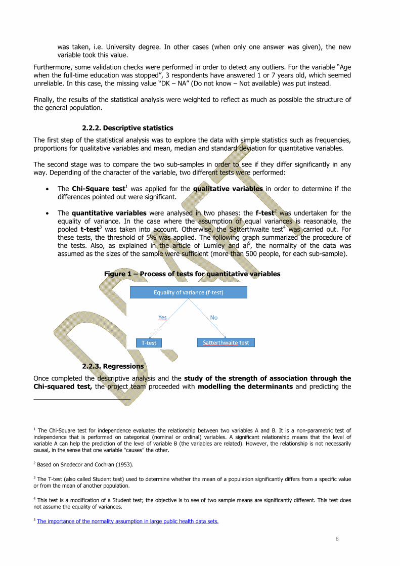
2.2.2. Descriptive statistics

The first step of the statistical analysis was to explore the data with simple statistics such as frequencies, proportions for qualitative variables and mean, median and standard deviation for quantitative variables.

The second stage was to compare the two sub-samples in order to see if they differ significantly in any way. Depending of the character of the variable, two different tests were performed:

• The Chi-Square test1 was applied for the qualitative variables in order to determine if the differences pointed out were significant.

• The quantitative variables were analysed in two phases: the f-test2 was undertaken for the equality of variance. In the case where the assumption of equal variances is reasonable, the pooled t-test3 was taken into account. Otherwise, the Satterthwaite test4 was carried out. For these tests, the threshold of 5% was applied. The following graph summarized the procedure of the tests. Also, as explained in the article of Lumley and al5, the normality of the data was assumed as the sizes of the sample were sufficient (more than 500 people, for each sub-sample).

Figure 1 – Process of tests for quantitative variables

2.2.3. Regressions

Once completed the descriptive analysis and the study of the strength of association through the Chi-squared test, the project team proceeded with modelling the determinants and predicting the

1 The Chi-Square test for independence evaluates the relationship between two variables A and B. It is a non-parametric test of independence that is performed on categorical (nominal or ordinal) variables. A significant relationship means that the level of variable A can help the prediction of the level of variable B (the variables are related). However, the relationship is not necessarily causal, in the sense that one variable “causes” the other.

2 Based on Snedecor and Cochran (1953).

3 The T-test (also called Student test) used to determine whether the mean of a population significantly differs from a specific value or from the mean of another population.

4 This test is a modification of a Student test; the objective is to see of two sample means are significantly different. This test does not assume the equality of variances.

5 The importance of the normality assumption in large public health data sets.

9

likelihood of an outcome with the help of the regression models. The three MEHM questions were taken into consideration as outcome variable in three different models:

• For the question HS.2, a binary logistic regression6 was performed to measure the probabilities to have a longstanding health problem according to several variables and to the particular the version of the questionnaire.

• The two other questions, evaluation of general health (HS.1) and limitation in the activities – GALI (HS.3/HS.4), were modelled through a Multinomial logistic regression7.

Moreover, the first MEHM question was analysed through an additional model, transforming the response in binary variable and using the Binary Logistic Regression.

Different indicators such as convergence, likelihood ratio, Akaike Information Criterion (AIC)8, and level of significance were presented for each model.

The variables included in each model were tested if they were significant, i.e. if they brought information to the model and also if there was no interaction between them. For each predictor, the Odds Ratio (OR), and the 95% confidence interval9 were reported. For each variable of interest, the reference group was defined as the most represented at a global level. The reference group for each variable was indicated in brackets.

2.2.4. Correction of the data

Finally, based on the results from the two previous parts (descriptive and regression analyses), a methodology was elaborated and suggested to be applied by data producers to correct backwards the time series.

6 The logit models, also called logistic regression are used to model dichotomous outcome variables, given one or more independent variables. In the logit model, the log odds of the outcome is modeled as a linear combination of the predictor variables. As with other types of regression, multinomial logistic regression can have nominal and/or continuous independent variables and can have interactions between independent variables to predict the dependent variable. The multinomial logistic regression coefficients are estimated for k-1 models, where k is the number of levels of the outcome variable. Therefore, each estimate listed in the result tables must be considered in terms both the parameter it corresponds to and the model to which it belongs (and the chosen reference category). The standard interpretation of the multinomial logit is that for a unit change in the predictor variable, the logit of outcome m relative to the referent group is expected to change by its respective parameter estimate (which is in log-odds units) given the other variables in the model are held constant.

7 The multinomial logistic regression is a classification method that generalizes logistic regression to multiclass problems, i.e. with more than two possible discrete outcomes. The setup is the same as in a logistic regression, the only difference being that the dependent variables are categorical rather than binary.

8 The AIC is a measure of the relative quality of a statistical model, for a given set of data. It deals with the trade-off between the goodness of fit of the model and the complexity of the model. It is calculated as AIC = -2 Log L + 2((k-1) + s), where k is the number of levels of the dependent variable and s is the number of predictors in the model. AIC is used for the comparison of models from different samples or non-nested models. Ultimately, the model with the smallest AIC is considered the best.

9 The interpretation of the CI are the following: at 95% of confidence that upon repeated trials, 95% of the CI’s would include the “true” population OR. It is equivalent to the Chi-Square test statistics: if the CI includes one, it means that the OR equals one, given the other predictors are in the model. The CI brings information on the prevision of the point estimate.

10

3. Results

3.1. Descriptive statistics on the two sub-samples

3.1.1. Socio-demographic characteristics

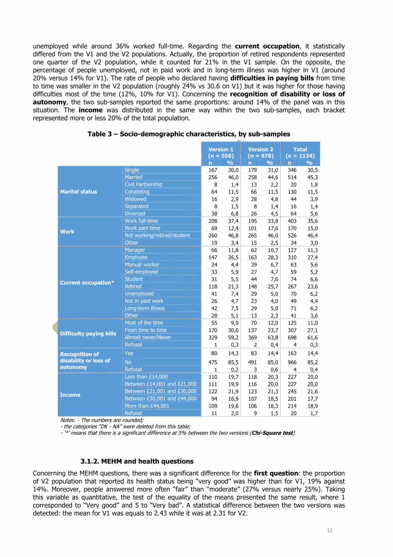
The sub-sample which received the V2 of the MEHM was slightly larger than the V1 sub-sample: 578 vs 556 respectively (due to the quality procedure and boost applied to the dataset). The proportions of men and women were the same in each sub-sample, with nearly 49% of men and 51% of women. Concerning the age, the V2 population was just 0.5 year older than the V1 one: an average age of 46.9 against 46.3 years old. Moreover, the percentage of people having more than 65 years old represented nearly one quarter of the V2 population, while in the V1 population it concerned one person out of 5. About the education, the majority of the population only had other formal qualifications, different from a university degree (around 57%). A slight difference appeared between the two sub-samples, not being statistically significant: more people had a university degree in V2 comparing with V1 (38% against roughly 36%). Regarding the degree of urbanisation, the difference between the two populations was statistically significant at 5% level: more people in V1 lived in small or middle-sized town than in V2 (46.3 vs 39.3%). On the contrary, less people lived in rural area or village in V1.

Table 2 – Demographic characteristics, by sub-samples

Version 1 (n = 556)

Version 2 (n = 578)

Total (n = 1134)

n % n % n %

Gender Men 272 48.9 282 48.8 554 48.9 Women 284 51.1 296 51.2 580 51.1

Age group

15-24 79 14.2 90 15.5 169 14.9 25-39 142 25.5 135 23.4 277 24.4 40-54 141 25.4 137 23.8 279 24.6 55-64 85 15.2 76 13.1 160 14.1 65+ 110 19.8 140 24.2 249 22.0

Education

At least university degree 163 36.4 166 37.9 329 37.2

Only other formal qualifications 255 57.2 247 56.2 502 56.7 No formal educational qualification 28 6.3 26 5.8 54 6.1

Region

North East 22 4.0 24 4.2 46 4.1 North West 64 11.5 62 10.7 126 11.1 Yorshire & Humberside 48 8.7 46 7.9 94 8.3 East Midlands 38 6.9 43 7.5 82 7.2 West Midlands 57 10.3 43 7.4 100 8.8 South West 51 9.2 45 7.8 96 8.5 East of England 48 8.7 57 9.9 105 9.3 London 68 12.3 78 13.5 146 12.9 South East 80 14.4 75 13.0 155 13.7 Wales 21 3.8 34 5.9 56 4.9 Scotland 45 8.2 51 8.8 96 8.5 Nothern Ireland 12 2.1 20 3.4 32 2.8

Degree of urbanisation*

Rural area or village 104 18.6 148 25.7 252 22.2 Small or middle-sized town 257 46.3 227 39.3 484 42.7 Large Town 195 35.1 203 35.1 398 35.1

Notes: - The numbers are rounded; - the categories "DK - NA" were deleted from this table; - '*' means that there is a significant difference at 5% between the two versions (Chi-Square test)

Continuing with the analysis of the socio-demographic variables, almost the majority of the panel was married (45%), and nearly one person out of three was single. Indeed, the marital status was distributed in the same proportion for the two sub-samples: no statistical difference was detected. The same observation could be noted for the working status. Not far from half of the panel was inactive or

11

unemployed while around 36% worked full-time. Regarding the current occupation, it statistically differed from the V1 and the V2 populations. Actually, the proportion of retired respondents represented one quarter of the V2 population, while it counted for 21% in the V1 sample. On the opposite, the percentage of people unemployed, not in paid work and in long-term illness was higher in V1 (around 20% versus 14% for V1). The rate of people who declared having difficulties in paying bills from time to time was smaller in the V2 population (roughly 24% vs 30.6 on V1) but it was higher for those having difficulties most of the time (12%, 10% for V1). Concerning the recognition of disability or loss of autonomy, the two sub-samples reported the same proportions: around 14% of the panel was in this situation. The income was distributed in the same way within the two sub-samples, each bracket represented more or less 20% of the total population.

Table 3 – Socio-demographic characteristics, by sub-samples

Version 1 (n = 556)

Version 2 (n = 578)

Total (n = 1134)

n % n % n %

Marital status

Single 167 30,0 179 31,0 346 30,5 Married 256 46,0 258 44,6 514 45,3 Civil Partnership 8 1,4 13 2,2 20 1,8 Cohabiting 64 11,5 66 11,5 130 11,5 Widowed 16 2,9 28 4,8 44 3,9 Separated 8 1,5 8 1,4 16 1,4 Divorced 38 6,8 26 4,5 64 5,6

Work

Work full-time 208 37,4 195 33,8 403 35,6 Work part-time 69 12,4 101 17,6 170 15,0 Not working/retired/student 260 46,8 265 46,0 526 46,4 Other 19 3,4 15 2,5 34 3,0

Current occupation*

Manager 66 11,8 62 10,7 127 11,3 Employee 147 26,5 163 28,3 310 27,4 Manual worker 24 4,4 39 6,7 63 5,6 Self-employed 33 5,9 27 4,7 59 5,2 Student 31 5,5 44 7,6 74 6,6 Retired 118 21,3 148 25,7 267 23,6 Unemployed 41 7,4 29 5,0 70 6,2 Not in paid work 26 4,7 23 4,0 49 4,4 Long-term illness 42 7,5 29 5,0 71 6,2 Other 28 5,1 13 2,3 41 3,6

Difficulty paying bills

Most of the time 55 9,9 70 12,0 125 11,0 From time to time 170 30,6 137 23,7 307 27,1 Almost never/Never 329 59,2 369 63,8 698 61,6 Refusal 1 0,3 2 0,4 4 0,3

Recognition of disability or loss of autonomy

Yes 80 14,3 83 14,4 163 14,4

No 475 85,5 491 85,0 966 85,2 Refusal 1 0,2 3 0,6 4 0,4

Income

Less than £14,000 110 19,7 118 20,3 227 20,0 Between £14,001 and £21,000 111 19,9 116 20,0 227 20,0 Between £21,001 and £30,000 122 21,9 123 21,3 245 21,6 Between £30,001 and £44,000 94 16,9 107 18,5 201 17,7 More than £44,001 109 19,6 106 18,3 214 18,9 Refusal 11 2,0 9 1,5 20 1,7


3.1.2. MEHM and health questions

Concerning the MEHM questions, there was a significant difference for the first question: the proportion of V2 population that reported its health status being “very good” was higher than for V1, 19% against 14%. Moreover, people answered more often “fair” than “moderate” (27% versus nearly 25%). Taking this variable as quantitative, the test of the equality of the means presented the same result, where 1 corresponded to “Very good” and 5 to “Very bad”. A statistical difference between the two versions was detected: the mean for V1 was equals to 2.43 while it was at 2.31 for V2.

12

Table 4 – MEHM questions, by sub-samples

Version 1 (n = 556)

Version 2 (n = 578)

Total (n = 1134)

n % n % n %

Health in general (Q6)*

Very good 80 14,4 112 19,3 192 16,9 Good 249 44,8 254 43,9 503 44,3 Fair/Moderate 152 27,3 143 24,8 295 26,0 Bad 56 10,1 61 10,6 117 10,3 Very bad 19 3,5 8 1,4 28 2,4

Having a longstanding illness (Q7)

Yes 233 42,1 262 45,6 496 43,9 No 321 57,9 313 54,4 634 56,1

Limited in their activities (Q8)(1)

Severely limited 58 10,5 55 9,5 113 10,0 Limited but not severely 172 31,1 149 25,9 321 28,4 Not limited at all 323 58,4 372 64,6 695 61,6


(1) For the Version 2, there was an additional routing question asking if the limitation was at least for the past 6 months. People answering "Severely limited" or "Limited but no severely" having "No" to this question were assigned to "Not limited at all".

For the two other questions, no statistical difference was found, even if small variations appeared between the two versions. As in the V2 additional specifications are presented in the second question, more people recorded having a longstanding illness: around 45% versus 42% in V1. For the GALI question – the third MEHM question, the proportion of people not limited in their activities was equal to nearly 65% in V2, whereas it corresponded to 58% of the V1 population. This slight disparity could be explained by those who answered “no” on the duration of limitation (at least the past 6 months) for in V2.

Table 5 - Difficulties in daily activities, by sub-samples

Version 1(n = 556)

Version 2 (n = 578)

Total (n = 1134)

n % n % n %

Difficulties in basic activities (Q12-Q18)

Severely limited 94 16.9 104 17.9 198 17.4Moderately limited 186 33.4 191 33.0 376 33.2Not limited 276 49.7 284 49.1 560 49.4

Note: the numbers are rounded.

The variable on the difficulties in basic activities, built thanks to Q12 to Q18, did not present a statistical difference between the two populations. In general, around 17% of the whole population was severely limited, while nearly one person out of two were not limited.

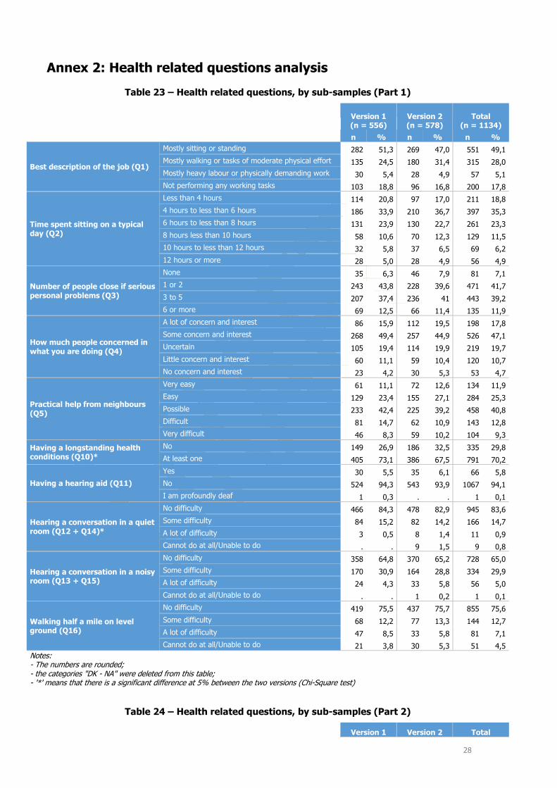
The table of the other health-related questions is available in the Annex 2.

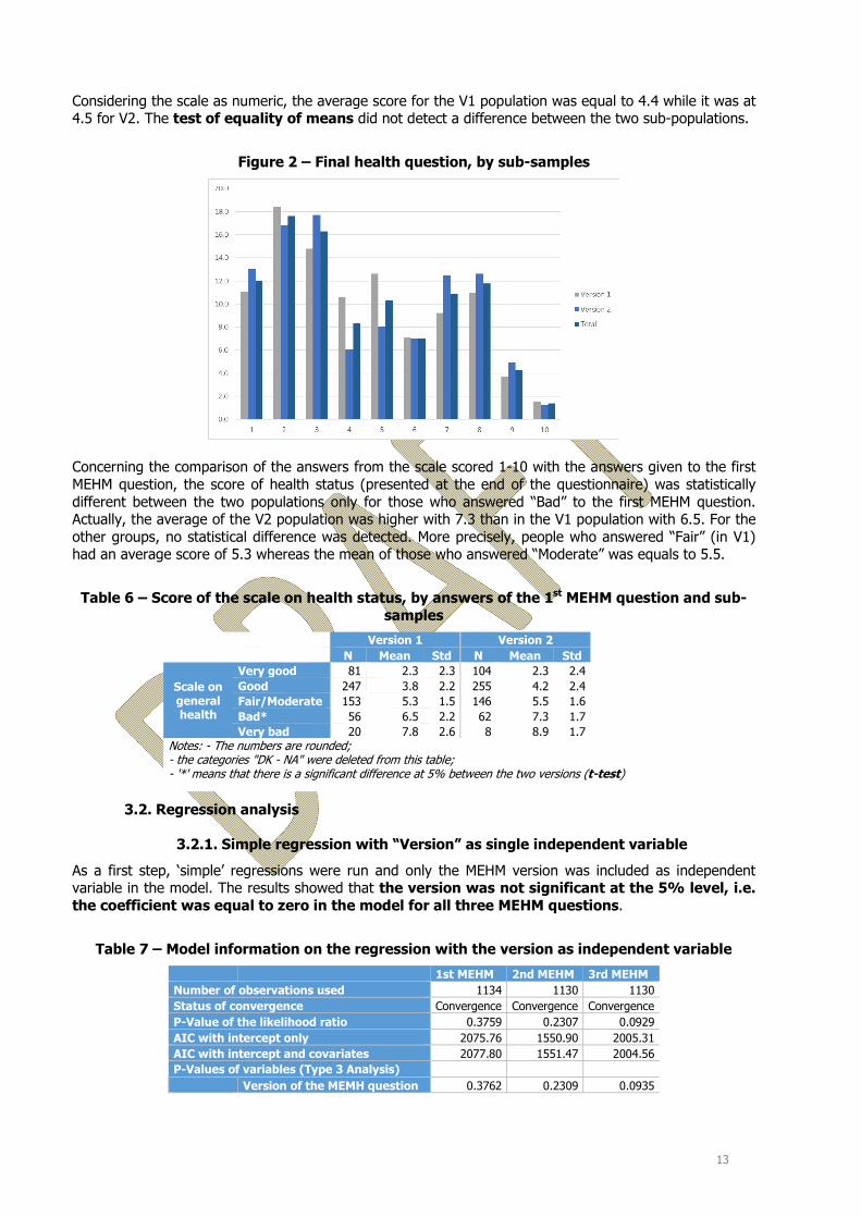
The final health question, the scale from 1 to 10 represented through the smileys (1=very good and 10=very bad), was statistically different from a sub-sample to another, at the level of 5%. For example, the scores “4” and “5” were more selected in the V1 population comparing with the V2 one (23.2% against 14.2% respectively). As presented in the figure below, the highest proportion recorded by the whole population was the item “2” (1 meant “Very good”). Around 35% of the panel reported a score higher or equal to 6.

However, the statistical difference identified previously should be carefully looked at. In fact, when the scores were gathered (1 with 2, 3 with 4, 5 with 6, 7 with 8 and 9 with 10), the chi-square test had a P-value equal to 0.13.

13

Considering the scale as numeric, the average score for the V1 population was equal to 4.4 while it was at 4.5 for V2. The test of equality of means did not detect a difference between the two sub-populations.

Figure 2 – Final health question, by sub-samples

Concerning the comparison of the answers from the scale scored 1-10 with the answers given to the first MEHM question, the score of health status (presented at the end of the questionnaire) was statistically different between the two populations only for those who answered “Bad” to the first MEHM question. Actually, the average of the V2 population was higher with 7.3 than in the V1 population with 6.5. For the other groups, no statistical difference was detected. More precisely, people who answered “Fair” (in V1) had an average score of 5.3 whereas the mean of those who answered “Moderate” was equals to 5.5.

Table 6 – Score of the scale on health status, by answers of the 1st MEHM question and sub-samples

Version 1 Version 2 N Mean Std N Mean Std

Scale on general health

Very good 81 2.3 2.3 104 2.3 2.4 Good 247 3.8 2.2 255 4.2 2.4 Fair/Moderate 153 5.3 1.5 146 5.5 1.6 Bad* 56 6.5 2.2 62 7.3 1.7 Very bad 20 7.8 2.6 8 8.9 1.7

Notes: - The numbers are rounded; - the categories "DK - NA" were deleted from this table; - '*' means that there is a significant difference at 5% between the two versions (t-test)

3.2. Regression analysis

3.2.1. Simple regression with “Version” as single independent variable

As a first step, ‘simple’ regressions were run and only the MEHM version was included as independent variable in the model. The results showed that the version was not significant at the 5% level, i.e. the coefficient was equal to zero in the model for all three MEHM questions.

Table 7 – Model information on the regression with the version as independent variable

1st MEHM 2nd MEHM 3rd MEHM Number of observations used 1134 1130 1130 Status of convergence Convergence Convergence Convergence P-Value of the likelihood ratio 0.3759 0.2307 0.0929 AIC with intercept only 2075.76 1550.90 2005.31 AIC with intercept and covariates 2077.80 1551.47 2004.56 P-Values of variables (Type 3 Analysis) Version of the MEMH question 0.3762 0.2309 0.0935

14

3.2.2. Regression models with multiple independent variables

All the details specified to the models such as the number of observations used, the AIC, the status of convergence, the p-values of the variables included in the model are available in the Annex 3.

First MEHM question as multinomial logistic regression

In order to perform the multinomial logistic regression, a pre-treatment of the data was performed. Indeed, the population who answered “Bad” to the question was equal to 28, which was too low to implement this analysis. Consequently, the categories “Very bad” and “bad” were gathered, such as “Very good” and “good”.

The first MEHM question was only associated with the difficulties in basic activities. The version of the MEHM questionnaire had no impact on the answers, as its p-value was at 0.20.

Table 8 – Odd ratios and their 95% CI for the 1st MEHM question, total population

Variable Class Odd Ratio 95% CI

Fair/Moderate vs very good + good

Gender [Woman] Man 1.04 [0.78;1.38]Version of the MEMH question [V2] V1 1.23 [0.92;1.63]Difficulties (Q12-Q18) [Severely limited]

Moderately limited 0.45 [0.29;0.70]Not limited 0.16 [0.10;0.25]

Bad + very bad vs very good + good



Note: the reference category is presented into brackets. The people who answered “Fair/Moderate” (against those with “Very good + good”) were less likely to be moderately limited or not limited at all in their basic activities, when controlling for the other variables. Those answered “Very bad” or “bad” (against “Very good” or “Good”) to the first MEHM question were also less likely to be moderately limited or not limited in their basic activities.

First MEHM question as binary outcome in logistic regression

An additional regression was performed, with only two modalities “Fair/Moderate” and “Very good/Good/Bad/Very bad”. The purpose of this was to see if the wording of the option “Fair/Moderate” had an impact. The table below presented the results of this logistic regression.

Table 9 – Odd ratios and their 95% CI for the 1st MEHM question considered as binary, total population

Variable Class Odd

Ratio 95% CI Gender [Woman] Man 0.98 [0.75;1.28]

Version of the MEMH question [V2] V1 0.87 [0.67;1.14]

Difficulties (Q12-Q18)

[Severely limited] Moderately limited 0.81 [0.56;1.18]

Not limited 2.02 [1.40;2.94] Notes: - The reference category is presented into brackets;- The probability of answered "Very good + good + bad + very bad" was modelled (against "Fair/Moderate")

Considering the question as binary, the conclusion for the versions of the questionnaire did not change: this variable had a p-value of 0.32. About the other variables, those not limited in their basic activities had a higher likelihood to pick an answer different to “Fair/Moderate”.

Second MEHM question

For this question, only one variable had a p-value inferior to 5% in the logistic regression: difficulties in basic activities.

15

Table 10 – Odd ratios and their 95% CI for the 2nd MEHM question, total population

Variable Class OddRatio

95% CI

Gender [Woman] Man 0.89 [0.68;1.16] Version of the MEMH question [V2] V1 0.85 [0.65;1.11] Difficulties (Q12-Q18)

[Severely limited]

Moderately limited 0.26 [0.17;0.40] Not limited 0.06 [0.04;0.09] Notes: - The reference category is presented into brackets;- The probability of answered "Having a longstanding illness" was modelled (against "Not having one longstanding illness")

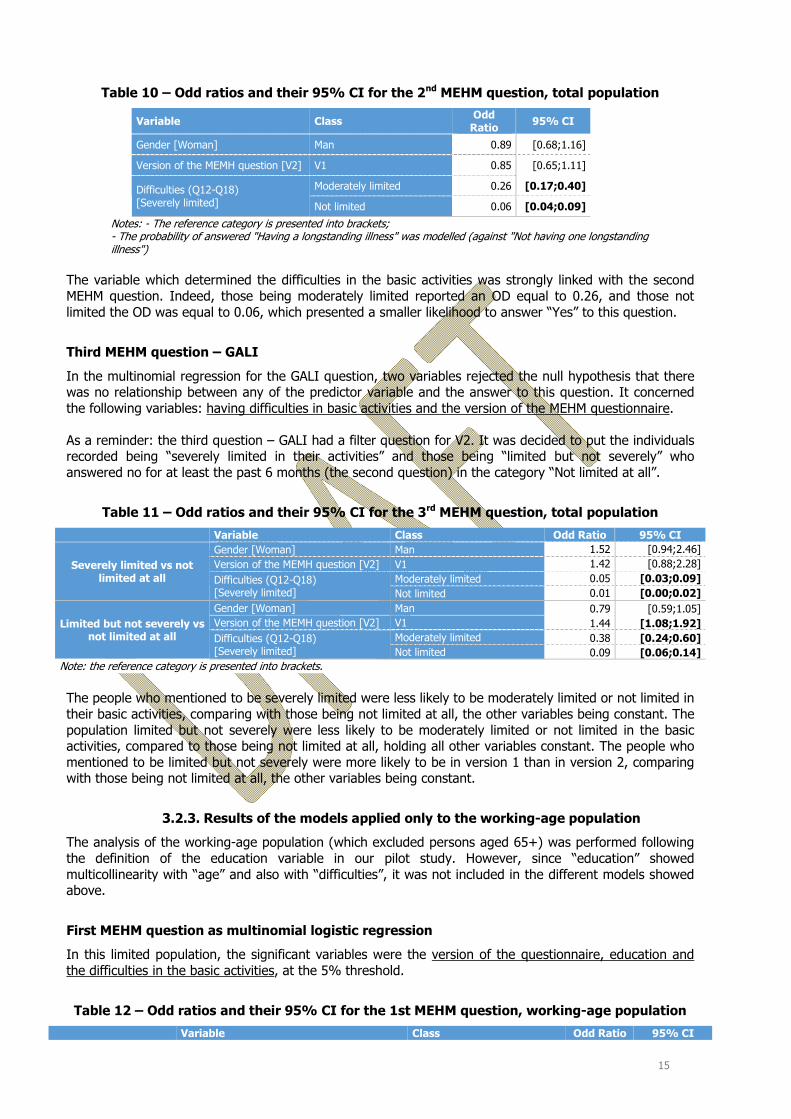
The variable which determined the difficulties in the basic activities was strongly linked with the second MEHM question. Indeed, those being moderately limited reported an OD equal to 0.26, and those not limited the OD was equal to 0.06, which presented a smaller likelihood to answer “Yes” to this question.

Third MEHM question – GALI

In the multinomial regression for the GALI question, two variables rejected the null hypothesis that there was no relationship between any of the predictor variable and the answer to this question. It concerned the following variables: having difficulties in basic activities and the version of the MEHM questionnaire.

As a reminder: the third question – GALI had a filter question for V2. It was decided to put the individuals recorded being “severely limited in their activities” and those being “limited but not severely” who answered no for at least the past 6 months (the second question) in the category “Not limited at all”.

Table 11 – Odd ratios and their 95% CI for the 3rd MEHM question, total population


Severely limited vs not limited at all

Gender [Woman] Man 1.52 [0.94;2.46]Version of the MEMH question [V2] V1 1.42 [0.88;2.28]

Difficulties (Q12-Q18) [Severely limited]


Limited but not severely vs not limited at all



Note: the reference category is presented into brackets.

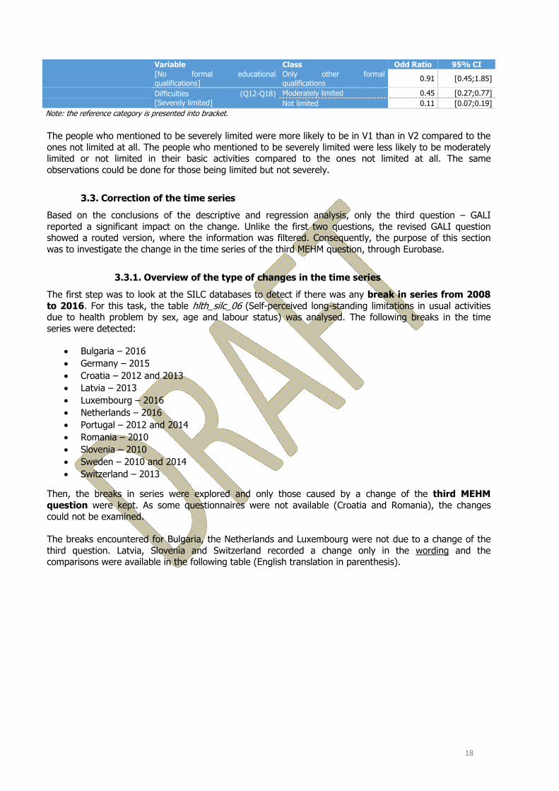
The people who mentioned to be severely limited were less likely to be moderately limited or not limited in their basic activities, comparing with those being not limited at all, the other variables being constant. The population limited but not severely were less likely to be moderately limited or not limited in the basic activities, compared to those being not limited at all, holding all other variables constant. The people who mentioned to be limited but not severely were more likely to be in version 1 than in version 2, comparing with those being not limited at all, the other variables being constant.

3.2.3. Results of the models applied only to the working-age population

The analysis of the working-age population (which excluded persons aged 65+) was performed following the definition of the education variable in our pilot study. However, since “education” showed multicollinearity with “age” and also with “difficulties”, it was not included in the different models showed above.

First MEHM question as multinomial logistic regression

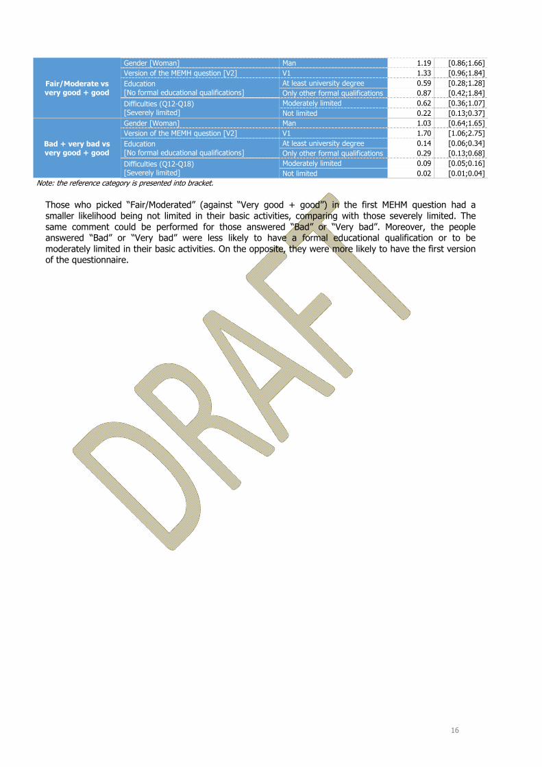
In this limited population, the significant variables were the version of the questionnaire, education and the difficulties in the basic activities, at the 5% threshold.

Table 12 – Odd ratios and their 95% CI for the 1st MEHM question, working-age population


16

Fair/Moderate vs very good + good

Gender [Woman] Man 1.19 [0.86;1.66]Version of the MEMH question [V2] V1 1.33 [0.96;1.84]Education [No formal educational qualifications]

At least university degree 0.59 [0.28;1.28]Only other formal qualifications 0.87 [0.42;1.84]



Bad + very bad vs very good + good


At least university degree 0.14 [0.06;0.34]Only other formal qualifications 0.29 [0.13;0.68]



Note: the reference category is presented into bracket.

Those who picked “Fair/Moderated” (against “Very good + good”) in the first MEHM question had a smaller likelihood being not limited in their basic activities, comparing with those severely limited. The same comment could be performed for those answered “Bad” or “Very bad”. Moreover, the people answered “Bad” or “Very bad” were less likely to have a formal educational qualification or to be moderately limited in their basic activities. On the opposite, they were more likely to have the first version of the questionnaire.

17

First MEHM question as binary outcome in logistic regression

Only the variable on the difficulties in basic activities had a p-value smaller than 5%.

Table 13 – Odd ratios and their 95% CI for the 1st MEHM question considered as binary, working-age population

Variable Class Odd Ratio 95% CI Gender [Woman] Man 0.85 [0.62;1.16]

Version of the MEMH question [V2] V1 0.84 [0.61;1.15]

Education

[No formal educational qualifications] At least university degree 1.04 [0.51;2.12]

Only other formal qualifications 0.80 [0.40;1.60] Difficulties (Q12-Q18)

[Severely limited] Moderately limited 0.59 [0.37;0.93]

Not limited 1.41 [0.90;2.22] Notes: - The reference category is presented into bracket;- The probability of answered "Very good + good + bad + very bad" was modelled (against "Fair/Moderate")

Those answered “Very good” or “good” or “bad” or “Very bad” were less likely to be moderately limited in their basic activities.

Second MEHM question

At the 5% threshold, the variable on the difficulties in basic activities was determinant.

Table 14 – Odd ratios and their 95% CI for the 2nd MEHM question, working-age population


Gender [Woman] Man 0.82 [0.60;1.11] Version of the MEMH question [V2] V1 0.81 [0.59;1.10] Education

[No formal educational qualifications]

At least university degree 0.66 [0.34;1.29] Only other formal qualifications 0.97 [0.50;1.86] Difficulties (Q12-Q18)

[Severely limited]

Moderately limited 0.28 [0.17;0.45] Not limited 0.06 [0.04;0.10] Notes: - The reference category is presented into bracket; - The probability of answered "Having a longstanding illness" was modelled (against "Not having one longstanding illness")

In the working-age population, the people who answered “Having a longstanding illness” in the second MEHM question had a smaller likelihood to be moderately limited or not limited in the basic activities.

Third MEHM question – GALI

Regarding the level of significance, two variables had a p-value smaller than 5%: the version of the MEHM questionnaire and the difficulties in basic activities.

Table 15 – Odd ratios and their 95% CI for the 3rd MEHM question, working-age population


Severely limited vs not limited at all


At least university degree 0.70 [0.24;2.03]Only other formal qualifications

0.58 [0.21;1.65]

Difficulties (Q12-Q18)[Severely limited]


Limited but not severely vs not limited at all

Gender [Woman] Man 0.86 [0.61;1.20]Version of the MEMH question [V2] V1 1.48 [1.06;2.07]Education At least university degree 0.61 [0.29;1.27]

18

Variable Class Odd Ratio 95% CI [No formal educational qualifications]

Only other formal qualifications

0.91 [0.45;1.85]

Difficulties (Q12-Q18)[Severely limited]


Note: the reference category is presented into bracket.

The people who mentioned to be severely limited were more likely to be in V1 than in V2 compared to the ones not limited at all. The people who mentioned to be severely limited were less likely to be moderately limited or not limited in their basic activities compared to the ones not limited at all. The same observations could be done for those being limited but not severely.

3.3. Correction of the time series

Based on the conclusions of the descriptive and regression analysis, only the third question – GALI reported a significant impact on the change. Unlike the first two questions, the revised GALI question showed a routed version, where the information was filtered. Consequently, the purpose of this section was to investigate the change in the time series of the third MEHM question, through Eurobase.

3.3.1. Overview of the type of changes in the time series

The first step was to look at the SILC databases to detect if there was any break in series from 2008 to 2016. For this task, the table hlth_silc_06 (Self-perceived long-standing limitations in usual activities due to health problem by sex, age and labour status) was analysed. The following breaks in the time series were detected:

• Bulgaria – 2016 • Germany – 2015 • Croatia – 2012 and 2013 • Latvia – 2013 • Luxembourg – 2016 • Netherlands – 2016 • Portugal – 2012 and 2014 • Romania – 2010 • Slovenia – 2010 • Sweden – 2010 and 2014 • Switzerland – 2013

Then, the breaks in series were explored and only those caused by a change of the third MEHM question were kept. As some questionnaires were not available (Croatia and Romania), the changes could not be examined.

The breaks encountered for Bulgaria, the Netherlands and Luxembourg were not due to a change of the third question. Latvia, Slovenia and Switzerland recorded a change only in the wording and the comparisons were available in the following table (English translation in parenthesis).

19

Table 16 – Wording change in the SILC questionnaire for LV, SI and CH

First version Second version Year Question Year Question

Latvia 2012 “Vai Jums pašreiz ir veselības problēmas, kas vismaz pēdējos 6 mēnešus ir traucējušas vai ierobežojušas Jūsu ikdienas aktivitātes mājās, darbā vai atpūtā?” (Do you currently have health problems that have disturbed or restricted your daily activities at home, at work or at rest for at least the last 6 months?)

2013 “Cik lielā mērā kāda veselības problēma vismaz pēdējo 6 mēnešu laikā ir Jūs ierobežojusi veikt aktivitātes, ko cilvēki parasti dara?” (To what extent has a health problem over the last 6 months been restricted to activities that people usually do?)

Slovenia 2009 “Ali je bila 'Ime Priimek (letnica)' v zadnjih 6 mesecih dlje časa oviran/-a pri običajnih dejavnostih zaradi zdravstvenih težav?” (Was' Last Name '(Year)' over the past 6 months disturbed for normal activities due to health problems?)

2010 “V kolikšni meri je 'Ime Priimek (letnica)' zadnjih 6 mesecev ali dlje oviran/-a zaradi zdravstvenih težav pri običajnih aktivnostih?” (To what extent is 'Last Name (Year)' for the last 6 months or longer hindered due to health problems in normal activities?)

Switzerland 2012 “Depuis au moins 6 mois, êtes-vous limité(e) par un problème de santé dans les activités que les gens font habituellement ? Si oui, dans quelle mesure?” (For at least 6 months, are you limited by a health problem in the activities that people usually do? If so, how?)

2013 “Depuis au moins 6 mois, dans quelle mesure êtes-vous limité/e par un problème de santé dans les activités que les gens font habituellement ? Diriez-vous que vous êtes... ” (For at least 6 months, how much are you limited by a health problem in the activities that people usually do? Would you say that you are ...)

Finally, only Germany, Portugal and Sweden reported a change of the collection of the GALI question which included the introduction of one or more filter questions.

20

3.3.2. Analysis of the changes

Germany

In 2014, the GALI question and answers were very similar to the one tested in the V1 of the present pilot study. However, the 2015 questionnaire was different than the V2 tested. Indeed, three questions were asked, instead of two. The first one was on the existence or not of a limitation in the daily activities. Then, the second question was about the severity of the limitations and the last question was on the duration of the limitations.

The question here is to know how the people limited (severely or not) have been classified according to the last question on duration of at least 6 months: how has the duration been taken into account? Have respondents being limited for less than 6 months been classified as “not limited at all”?

21

Portugal

Portugal made two changes, one in 2012 and another in 2014. For the first change in 2012, a filter question was introduced. Comparing to the change evaluated in the pilot study in the UK, the question was differently asked. Indeed, first the interviewee should answer if he/she was limited for at least the last 6 months. If the answer was yes, he/she had to evaluate the level of limitation.

For the second change in 2014, only one question was asked but it was different from the one in 2011. Actually, this version was closer to the V1 tested, than the one provided until 2011.

22

Sweden

Until 2013, Sweden had a unique question for GALI, which was similar to the question asked in the V1 population. In 2014, 4 questions were created and the way of asking was different from the V2 in the study. Two filter questions were introduced: the first asked if the interviewee encountered difficulties in daily life, and the second was on the nature of the limitations.

As for Germany, the question is to know how people who answered “no” to the last question concerning the duration of at least six months were classified.

23

3.3.3. Analysis of the data from Eurobase

The time series showed that when the GALI question was differently asked, introducing one or more routing questions, the percentage of people having some or severe limitations decreased.

Table 17 – Percentage of people being “limited, but not severely”

2008 2009 2010 2011 2012 2013 2014 2015 2016

Rate of Change between the two versions

DE (1) 22.5 22.1 21.6 22.3 23.2 24.0 25.5 14.1 14.1 -44.7% SE (2) 14.1 13.4 13.5 14.5 : 14.3 9.0 9.1 8.9 -37.1% PT (3) 18.2 21.2 22.1 20.3 15.9 16.6 26.0 26.7 24.8 -21.7% Note: the numbers in bold are those where a filter question was added (1) Change calculated between 2014 and 2015 (2) Change calculated between 2013 and 2014 (3) Change calculated between 2011 and 2012

For Germany, the proportion of people having some limitations was at 25.5% in 2014 and fell at 14% in 2015. In Portugal, in 2012 and 2013, the percentage was around 16% (which represented a 5 percentage points decrease from 2011) and increased again in 2014 to 26%. In Sweden, the proportion was equal to 14% in 2013 and at 9% after the change in 2014.

Table 18 – Percentage of people being “severely limited”

2008 2009 2010 2011 2012 2013 2014 2015 2016

Rate of Change between the two versions

DE (1) 10.6 10.1 10.2 10.0 10.9 10.4 10.7 7.1 7.3 -33.6% SE (2) 9.0 8.0 8.4 8.1 : 7.7 3.8 3.7 3.7 -50.6% PT (3) 12 10.9 9.4 9.3 9 9.3 9.2 9.5 8.3 -3.2% Note: the numbers in bold are those where a filter question was added (1) Change calculated between 2014 and 2015 (2) Change calculated between 2013 and 2014 (3) Change calculated between 2011 and 2012

In Sweden, the proportion of those being severed limited halved, from 7.7% in 2013 to 3.8% in 2014. On the opposite, the percentage of those being severed limited remained stable with the change of questionnaires, around 9%.

To conclude, it seemed that the impact of the filter question was more significant for those having some limitations. One explanation would be that the question on the duration allowed interviewees to better understand this information. Moreover, those being severely limited were generally so for more than 6 months.

3.3.4. Suggestion of a correction method

The method that is suggested and applied in this section is specific to each country and follows these steps:

1. Calculation of the trend for the time series where the “non-routed” question was observed (similarly to version 1 of the pilot study), using a linear regression;

2. With the equation obtained by linear regression, calculation of the data for the years where the filter question was introduced, so obtaining a theoretical value;

3. Calculation of the change between the observed and theoretical values; 4. Calculation of the average of the changes (in case of multiple values available, otherwise the

single data point was taken into consideration);

24

5. Application of the average change in the “old” time series to obtain the new value.

This method included these assumptions:

• The trend of the time series was linear; • The calculations were done on a global basis on all the population, not specific to one group; • The percentage change calculated was constant in time.

One advantage of this method was that it was applicable to all the possible trends in the time series. In fact, even if the introduction of the filter question had caused an increase of the number of people answering severely limited or limited but not severely (so an opposite case to the one actually recorded), this approach would work as well. In the table below the trend for the three countries is analysed and a decreasing proportion of people being limited (severely or not) is observed.

The following tables present the time series where the methodology described below was applied.

Table 19 – Suggestion of the correction backward, for people declared being severely limited

2008 2009 2010 2011 2012 2013 2014 2015 2016 DE 7.2 6.9 6.9 6.8 7.4 7.1 7.3 7.1 7.3 SE 4.6 4.1 4.3 4.2 : 4.0 3.8 3.7 3.7 PT (1) 14.7 13.4 11.5 11.4 9 9.3 9.2 9.5 8.3 Note: the numbers in red italics are those where the correction was applied (1) The data from 2014 to 2016 were not used in this process

Table 20– Suggestion of the correction backward, for people declared being limited but not severely

2008 2009 2010 2011 2012 2013 2014 2015 2016 DE 12.5 12.3 12.0 12.4 12.9 13.3 14.2 14.1 14.1 SE 8.7 8.3 8.4 9.0 : 8.9 9.0 9.1 8.9 PT (1) 13.1 15.2 15.9 14.6 15.9 16.6 26 26.7 24.8 Note: the numbers in red italics are those where the correction was applied (1) The data from 2014 to 2016 were not used in this process

The results obtained by this method for Germany and Sweden showed coherent time series. Indeed, the data between 2008 and 2014 for Germany were in the same order of magnitude than the following years.

However, the results for Portugal were not as good as for the two other countries. In fact, only four data points were used to determine the coefficients of the linear regression, which was not enough to have reliable estimations. Moreover, the questionnaire changed in 2014 to come back to one question (which was different to the one asked before 2012), and these data could not be taken into account.

25

4. Discussion This project provided some information regarding the change in the MEHM questionnaire. This study was based on 1,134 respondents in the UK, distributed in two sub-samples comparable in terms of demographic characteristics. The two versions of the questionnaire were tested and compared: the two first questions did not note a statistical change between the two sub-samples. Due to a filter question, the third question reported a decrease in the proportion of the people being limited but not severely. It could be explained as the additional question, on the duration of limitation (at least 6 months) allowed the respondents to better determine the degree of their limitations.

Nevertheless, several reserves could be mentioned on this study.

The design of the study could be uncertain on certain points. Indeed, an Internet study rose the question on the access for the neediest, for the elderly and for those having limitations that could prevent to answer to this questionnaire, for example. Additionally, a panel was used to collect the data, i.e. the respondents received some money against their answers. It could put some doubts on the representativeness of the population, even if quotas were created and applied.

Regarding the final health question, this scale from 1 to 10 had some limitations. Firstly, as it was not asked following the MEHM questions, it could happen than the participants had a different view about their health status. Secondly, 1 was defined as “Very good” and 10 as “Very bad”, depending of the culture and personal perception, the numbers could be considered in the other way: 1 as being “Very bad” and 10 “Very good”. In this perspective, outliers were defined as following:

• 1st MEHM question = Very good and Q27 >= 8; • 1st MEHM question = good and Q27 >= 9; • 1st MEHM question = Bad and Q27 <= 3; • 1st MEHM question = Very bad and Q27 <= 2.

Table 21 – Distribution of the outliers for the final health question, by sub-sample

Version 1 (n = 556)

Version 2 (n = 578)

Total (n = 1134)

n % n % n % No outlier 538 96.8 556 96.1 1094 96.4

Outlier 18 3.2 22 3.9 40 3.6

Note: The numbers are rounded.

The outliers were distributed in the same proportion for each sub-sample. Thirdly, the uses of the smileys could questionable on the seriousness of the study, as for the elderly, it could be not intuitive.

Finally, here the English version was tested, and depending on the translations in each country, the impact of the changes could be different. The main issue will be to stay closer as much as possible to the wording tested in this study, in order to compare the results obtained with those presented in this document.

26

ANNEXES

27

Annex 1

Table 22 – Distribution of the quotas variables, weighted and unweighted

28

Annex 2: Health related questions analysis

Table 23 – Health related questions, by sub-samples (Part 1)

Version 1 (n = 556)

Version 2 (n = 578)

Total (n = 1134)

n % n % n %

Best description of the job (Q1)

Mostly sitting or standing 282 51,3 269 47,0 551 49,1Mostly walking or tasks of moderate physical effort 135 24,5 180 31,4 315 28,0Mostly heavy labour or physically demanding work 30 5,4 28 4,9 57 5,1Not performing any working tasks 103 18,8 96 16,8 200 17,8

Time spent sitting on a typical day (Q2)

Less than 4 hours 114 20,8 97 17,0 211 18,84 hours to less than 6 hours 186 33,9 210 36,7 397 35,36 hours to less than 8 hours 131 23,9 130 22,7 261 23,38 hours less than 10 hours 58 10,6 70 12,3 129 11,510 hours to less than 12 hours 32 5,8 37 6,5 69 6,212 hours or more 28 5,0 28 4,9 56 4,9

Number of people close if serious personal problems (Q3)

None 35 6,3 46 7,9 81 7,11 or 2 243 43,8 228 39,6 471 41,73 to 5 207 37,4 236 41 443 39,26 or more 69 12,5 66 11,4 135 11,9

How much people concerned in what you are doing (Q4)

A lot of concern and interest 86 15,9 112 19,5 198 17,8Some concern and interest 268 49,4 257 44,9 526 47,1Uncertain 105 19,4 114 19,9 219 19,7Little concern and interest 60 11,1 59 10,4 120 10,7No concern and interest 23 4,2 30 5,3 53 4,7

Practical help from neighbours (Q5)

Very easy 61 11,1 72 12,6 134 11,9Easy 129 23,4 155 27,1 284 25,3Possible 233 42,4 225 39,2 458 40,8Difficult 81 14,7 62 10,9 143 12,8Very difficult 46 8,3 59 10,2 104 9,3

Having a longstanding health conditions (Q10)*

No 149 26,9 186 32,5 335 29,8At least one 405 73,1 386 67,5 791 70,2

Having a hearing aid (Q11)

Yes 30 5,5 35 6,1 66 5,8No 524 94,3 543 93,9 1067 94,1I am profoundly deaf 1 0,3 . . 1 0,1

Hearing a conversation in a quiet room (Q12 + Q14)*

No difficulty 466 84,3 478 82,9 945 83,6Some difficulty 84 15,2 82 14,2 166 14,7A lot of difficulty 3 0,5 8 1,4 11 0,9Cannot do at all/Unable to do . . 9 1,5 9 0,8

Hearing a conversation in a noisy room (Q13 + Q15)

No difficulty 358 64,8 370 65,2 728 65,0Some difficulty 170 30,9 164 28,8 334 29,9A lot of difficulty 24 4,3 33 5,8 56 5,0Cannot do at all/Unable to do . . 1 0,2 1 0,1

Walking half a mile on level ground (Q16)

No difficulty 419 75,5 437 75,7 855 75,6Some difficulty 68 12,2 77 13,3 144 12,7A lot of difficulty 47 8,5 33 5,8 81 7,1Cannot do at all/Unable to do 21 3,8 30 5,3 51 4,5


Table 24 – Health related questions, by sub-samples (Part 2)

Version 1 Version 2 Total

29

(n = 556) (n = 578) (n = 1134)

n % n % n %

Walking up or down 12 steps (Q17)


Washing all over or dressing (Q18)


Experienced delay in getting health care because of time to obtain an appointment (Q19)

Yes 105 18,9 121 21,1 226 20,0No 339 61,1 322 56,0 660 58,5No need 111 20,0 132 22,9 243 21,5

Experienced delay in getting health care due to distance or transport problem (Q20)

Yes 38 6,8 40 7,0 78 6,9No 387 69,7 399 69,0 786 69,3No need 131 23,6 139 24,1 270 23,8

Needed medical care but could not afford it (Q21)

Yes 24 4,3 43 7,4 67 5,9No 394 70,9 385 66,6 779 68,7No need 138 24,9 150 26,0 288 25,4

Needed dental care but could not afford it (Q22)

Yes 79 14,2 73 12,7 152 13,4No 395 71,1 408 70,8 803 70,9No need 82 14,8 95 16,5 177 15,7

Needed prescribed medicines but could not afford it (Q23)

Yes 29 5,2 36 6,2 65 5,7No 427 76,8 425 73,6 852 75,1No need 100 18,0 117 20,2 217 19,2

Smoking behaviour

Currently smoke regurarly 80 14,5 99 17,1 179 15,8Currently smoke occasionnaly 43 7,7 33 5,6 75 6,6Used to smoke but stop 158 28,5 163 28,3 322 28,4Never smoke 270 48,6 278 48,2 548 48,4Refusal 5 0,9 5 0,9 10 0,9

Body Mass Index

Underweight 51 12,4 50 11,6 101 12,0Normal weight 154 37,5 165 38,7 320 38,1Overweight 121 29,3 126 29,5 247 29,4Obese 86 20,8 86 20,1 172 20,5


30

Annex 3: Regression models information

Table 25 – Information on the regression models on total population

1st MEHM 1st MEHM - binary 2nd MEHM 3rd MEHM Number of observations used 1134 1134 1130 1130Status of convergence Convergence Convergence Convergence ConvergenceP-Value of the likelihood ratio <0.0001 <0.0001 <0.0001 <0.0001AIC with intercept only 2075.76 1301.66 1550.90 2005.31AIC with intercept and covariates 1794.15 1270.39 1300.08 1643.78P-Values of variables (Type 3 Analysis)

Gender 0.9494 0.8724 0.3734 0.0156Version of the MEMH question 0.2012 0.3176 0.2301 0.0394Difficulties (Q12-Q18) <0.0001 <0.0001 <0.0001 <0.0001

Table 26 – Information on the regression models on the working-age population

1st MEHM 1st MEHM - binary 2nd MEHM 3rd MEHM Number of observations used 878 878 876 875Status of convergence Convergence Convergence Convergence ConvergenceP-Value of the likelihood ratio <0.0001 <0.0001 <0.0001 <0.0001AIC with intercept only 1615.02 983.79 1186.36 1540.01AIC with intercept and covariates 1388.28 966.44 987.77 1288.67P-Values of variables (Type 3 Analysis)

Gender 0.5547 0.3046 0.2018 0.3024Version of the MEMH question 0.05 0.27 0.1772 0.0236Education 0.0002 0.2869 0.0607 0.1084Difficulties (Q12-Q18) <0.0001 <0.0001 <0.0001 <0.0001

Documents

ITEM 5.1: ESTAT STUDY ON THE IMPACT OF CHANGES TO THE … EHIS... · • A global variable for each question of the MEHM question: the first and the second questions were identical