ISSN 1045-6333

HOUSEHOLD SPECIALIZATIONAND THE MALE MARRIAGE

WAGE PREMIUM

Joni HerschLeslie S. Stratton

Discussion Paper No. 298

10/2000

Harvard Law SchoolCambridge, MA 02138

The Center for Law, Economics, and Business is supported bya grant from the John M. Olin Foundation.

This paper can be downloaded without charge from:

The Harvard John M. Olin Discussion Paper Series:http://www.law.harvard.edu/programs/olin_center/

1

JEL Class: D13, J22, J31

HOUSEHOLD SPECIALIZATION AND THE MALE MARRIAGE WAGE PREMIUM

JONI HERSCH and LESLIE S. STRATTON*

Industrial and Labor Relations Review 54(1), October 2000, 78-94.

Abstract

Empirical research has consistently shown that married men have substantially higher wages,on average, than otherwise similar unmarried men. One commonly cited hypothesis to explainthis pattern is that marriage allows one spouse to specialize in market production and the other tospecialize in home production, enabling the former – usually the husband – to acquire moremarket-specific human capital and, ultimately, earn higher wages. The authors test thishypothesis using panel data from the National Survey of Families and Households. The datareveal that married men spent virtually the same amount of time on home production as didsingle men, albeit on different types of housework. Estimates from a fixed effects wage equationindicate that the male marriage wage premium is not substantially affected by controls for homeproduction activities. Household specialization, the authors conclude, does not appear to havebeen responsible for the marriage premium in this sample.

* Joni Hersch is Lecturer on Law at Harvard Law School and Leslie Stratton is AssistantProfessor of Economics at Virginia Commonwealth University.

2

Household Specialization and the Male Marriage Wage Premium

Joni Hersch and Leslie S. Stratton*

© 2000 Joni Hersch and Leslie S. Stratton. All rights reserved.

Virtually all wage regressions including an indicator of marital status find that married men

have substantially higher wages than do not-married men, even after controlling for observable

human capital and job characteristics. The magnitude varies but is quite large, with typical

values indicating that married men receive a wage premium of between ten and thirty percent.

While the empirical evidence of a marriage premium for men is incontrovertible, the precise

nature of the relation has not yet been convincingly explained. A leading theory is that

specialization within the household results in genuine productivity differences between married

men who have the opportunity to specialize and unmarried men who do not. Lacking direct

measures of specialization and time allocation, studies have used wife’s employment status as a

proxy for specialization, and ensuing results have been inconsistent.

An important contribution of this paper is the use of more direct measures of time allocation

to control for specialization within the household. We use panel data from the National Survey

of Families and Households that includes information on time allocated to nine different home

production activities. With these data we directly analyze whether the observed marriage

premium is due to specialization within the household. Our results indicate that specialization is

not responsible for the marriage premium.

*Joni Hersch is Lecturer on Law at Harvard Law School and Leslie Stratton is Assistant Professor of Economics atVirginia Commonwealth University. A data appendix with additional results and copies of the computer programsused to generate the results presented in the paper are available from Leslie Stratton at the Department of Economics,Virginia Commonwealth University, Richmond VA 23284-4000.

3

Background

Two primary explanations have been advanced regarding the wage premium for married

men.1 One is that more productive men marry, and the other is that marriage makes men more

productive.2 If more productive men marry, then men who marry should be more productive and

receive higher wages throughout their lifetime. In this case, marriage is serving as a proxy for

unobserved characteristics that are correlated with productivity, and the marital wage differential

is attributable to selection. If, on the other hand, marriage makes men more productive, then

wages should increase following marriage.

There is a substantial literature that examines these competing hypotheses and the source of

the underlying productivity differential. If more productive men are selected into marriage, then

marriage and wages are jointly endogenous. Using instrumental variables estimation on a cross-

section of data to control for this possible joint endogeneity, Nakosteen and Zimmer (1987) find

that the magnitude of the marriage premium is unchanged but that it becomes statistically

insignificant, a finding they interpret as evidence that the marriage premium is due to selection.

However, it is difficult to find suitable instruments for marriage and findings based on weak or

invalid instruments are suspect. Recent investigations have used panel data to estimate fixed

effects models, thereby netting out any unobserved individual-specific fixed effect that may be

1 Excellent surveys of the literature specifically examining the premium appear in Korenman and Neumark (1991)

and in Loh (1996).

2 An alternative explanation is that married men are more likely to choose jobs with undesirable and hence wage

compensating characteristics (Reed and Harford 1989). However, Hersch (1991) reports a significant marital wage

differential even after controlling for job characteristics.

4

correlated with both marriage and wages. Using this approach, Korenman and Neumark (1991)

conclude that at most twenty percent of the observed premium is due to selection. Other

researchers (Cornwell and Rupert 1997, Daniel 1991, Gray 1997) also report finding a marriage

premium in fixed effects estimates, though often of a smaller magnitude than that found by

Korenman and Neumark. An alternative selection mechanism, for which fixed effects models

would not correct, posits that men with more rapid wage growth (rather than men with higher

wage levels) may be more likely to marry. Both Korenman and Neumark (1991) and Gray

(1997) test for but find no evidence of such selection.

If marriage somehow makes men more productive, one possible implication is that men who

have been married longer receive higher wages. In fact, Kenny (1983), Korenman and Neumark

(1991), and Daniel (1991) find faster wage growth for married men, particularly early in

marriage. Cornwell and Rupert (1997) contest these findings, but overall the evidence tends to

support the productivity hypothesis.

Although the empirical evidence supports the hypothesis that marriage enhances

productivity, the causal mechanism is less clear. The theory most often referenced is Becker’s

theory of the family (1991). According to this theory, it is efficient for one spouse to specialize

in market production and the other to specialize in home production. The spouse (usually the

husband) who devotes more time to market production will acquire more market-specific human

capital, which will lead to an increase in market productivity and thereby to higher wages.

A number of other arguments can also be made linking marriage, specialization, and wages.

Becker’s (1985) model of effort posits that total effort is limited and any effort allocated to

housework reduces the effort available for market work. If increased effort means increased

productivity and increased wages, then men may benefit from specialization because they are

5

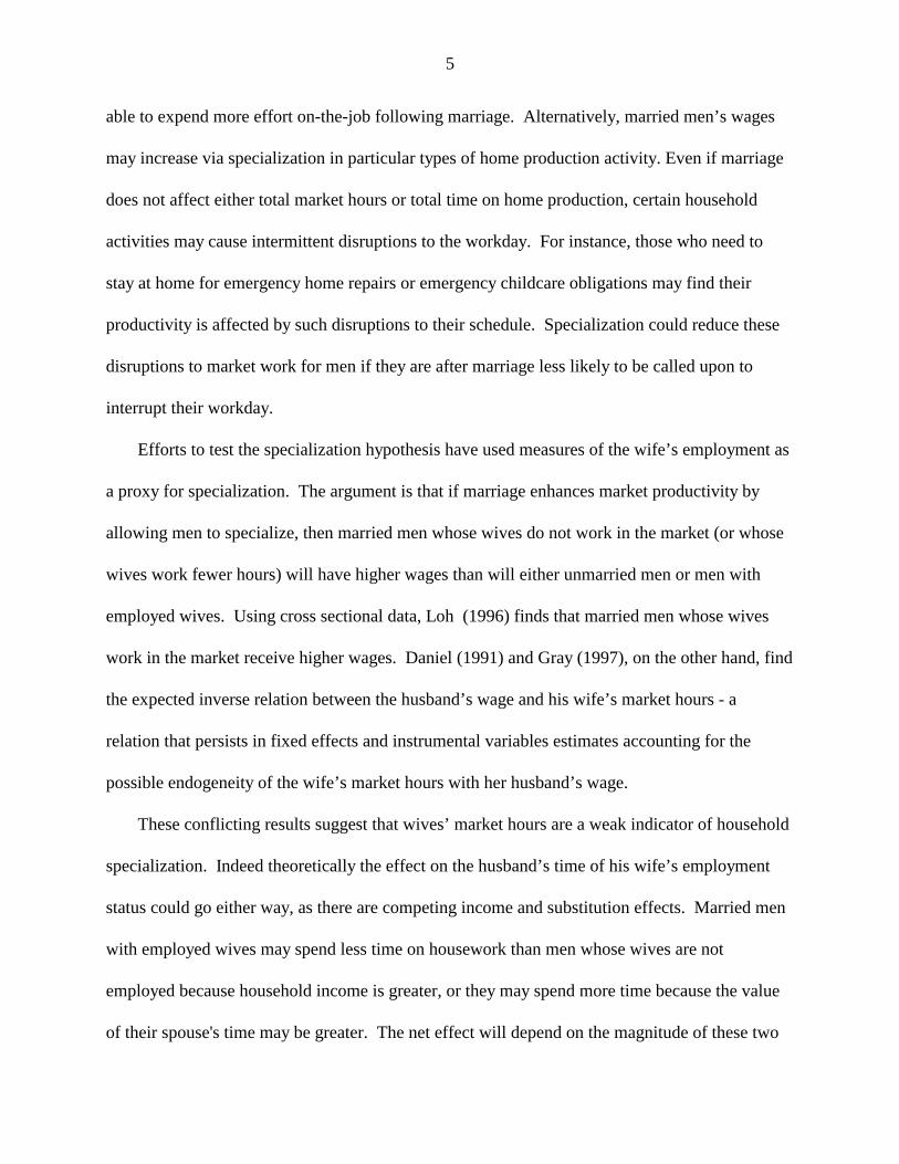
able to expend more effort on-the-job following marriage. Alternatively, married men’s wages

may increase via specialization in particular types of home production activity. Even if marriage

does not affect either total market hours or total time on home production, certain household

activities may cause intermittent disruptions to the workday. For instance, those who need to

stay at home for emergency home repairs or emergency childcare obligations may find their

productivity is affected by such disruptions to their schedule. Specialization could reduce these

disruptions to market work for men if they are after marriage less likely to be called upon to

interrupt their workday.

Efforts to test the specialization hypothesis have used measures of the wife’s employment as

a proxy for specialization. The argument is that if marriage enhances market productivity by

allowing men to specialize, then married men whose wives do not work in the market (or whose

wives work fewer hours) will have higher wages than will either unmarried men or men with

employed wives. Using cross sectional data, Loh (1996) finds that married men whose wives

work in the market receive higher wages. Daniel (1991) and Gray (1997), on the other hand, find

the expected inverse relation between the husband’s wage and his wife’s market hours - a

relation that persists in fixed effects and instrumental variables estimates accounting for the

possible endogeneity of the wife’s market hours with her husband’s wage.

These conflicting results suggest that wives’ market hours are a weak indicator of household

specialization. Indeed theoretically the effect on the husband’s time of his wife’s employment

status could go either way, as there are competing income and substitution effects. Married men

with employed wives may spend less time on housework than men whose wives are not

employed because household income is greater, or they may spend more time because the value

of their spouse's time may be greater. The net effect will depend on the magnitude of these two

6

components. By using spousal employment as a proxy for household specialization, researchers

assume that the substitution effect dominates the income effect. However, research by South and

Spitze (1994) indicates that the time allocated to home production by husbands whose wives are

employed is not substantially different from the time allocated by husbands whose wives are not

employed.

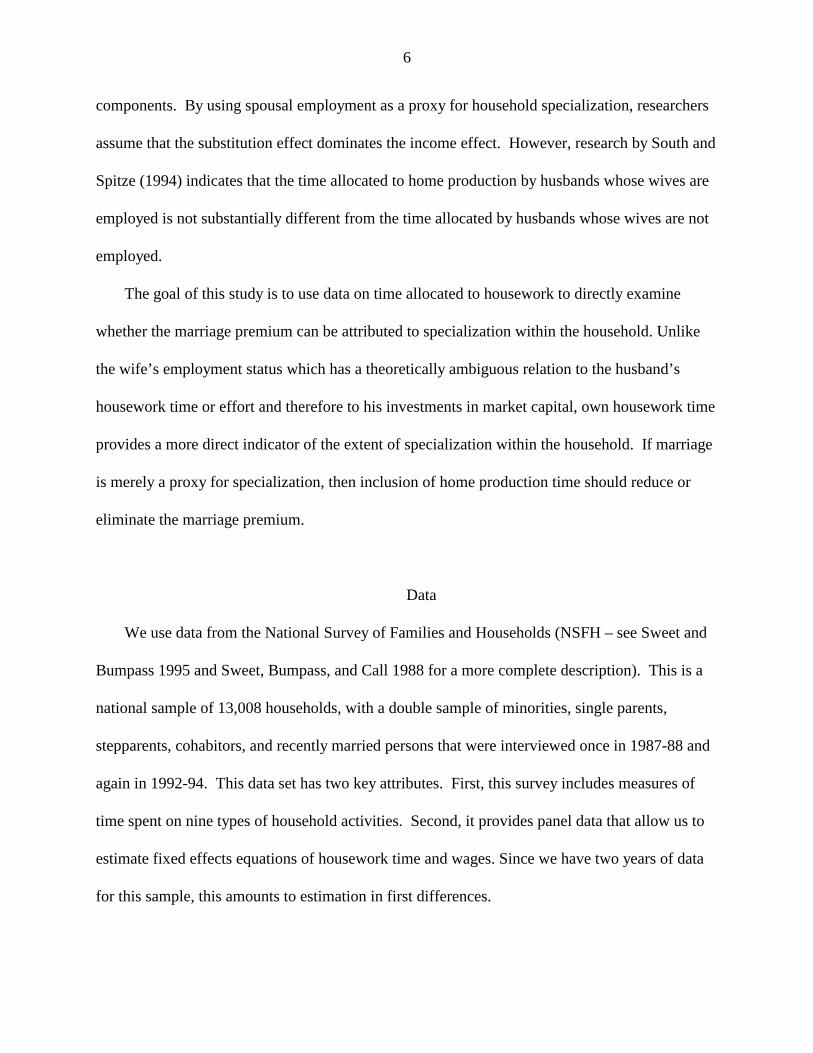
The goal of this study is to use data on time allocated to housework to directly examine

whether the marriage premium can be attributed to specialization within the household. Unlike

the wife’s employment status which has a theoretically ambiguous relation to the husband’s

housework time or effort and therefore to his investments in market capital, own housework time

provides a more direct indicator of the extent of specialization within the household. If marriage

is merely a proxy for specialization, then inclusion of home production time should reduce or

eliminate the marriage premium.

Data

We use data from the National Survey of Families and Households (NSFH – see Sweet and

Bumpass 1995 and Sweet, Bumpass, and Call 1988 for a more complete description). This is a

national sample of 13,008 households, with a double sample of minorities, single parents,

stepparents, cohabitors, and recently married persons that were interviewed once in 1987-88 and

again in 1992-94. This data set has two key attributes. First, this survey includes measures of

time spent on nine types of household activities. Second, it provides panel data that allow us to

estimate fixed effects equations of housework time and wages. Since we have two years of data

for this sample, this amounts to estimation in first differences.

7

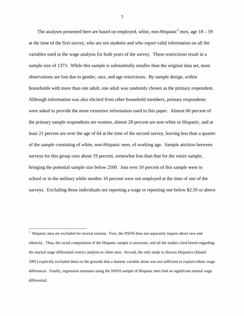
The analyses presented here are based on employed, white, non-Hispanic3 men, age 18 – 59

at the time of the first survey, who are not students and who report valid information on all the

variables used in the wage analysis for both years of the survey. These restrictions result in a

sample size of 1373. While this sample is substantially smaller than the original data set, most

observations are lost due to gender, race, and age restrictions. By sample design, within

households with more than one adult, one adult was randomly chosen as the primary respondent.

Although information was also elicited from other household members, primary respondents

were asked to provide the more extensive information used in this paper. Almost 60 percent of

the primary sample respondents are women, almost 28 percent are non-white or Hispanic, and at

least 21 percent are over the age of 64 at the time of the second survey, leaving less than a quarter

of the sample consisting of white, non-Hispanic men, of working age. Sample attrition between

surveys for this group runs about 19 percent, somewhat less than that for the entire sample,

bringing the potential sample size below 2500. Just over 10 percent of this sample were in

school or in the military while another 10 percent were not employed at the time of one of the

surveys. Excluding those individuals not reporting a wage or reporting one below $2.50 or above

3 Hispanic men are excluded for several reasons. First, the NSFH does not separately inquire about race and

ethnicity. Thus, the racial composition of the Hispanic sample is uncertain, and all the studies cited herein regarding

the marital wage differential restrict analysis to white men. Second, the only study to discuss Hispanics (Daniel

1991) explicitly excluded them on the grounds that a dummy variable alone was not sufficient to explain ethnic wage

differences. Finally, regression estimates using the NSFH sample of Hispanic men find no significant marital wage

differential.

8

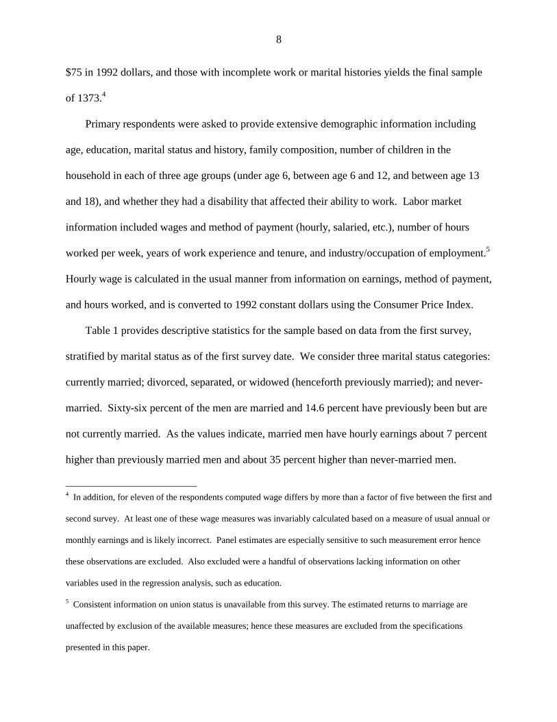
$75 in 1992 dollars, and those with incomplete work or marital histories yields the final sample

of 1373.4

Primary respondents were asked to provide extensive demographic information including

age, education, marital status and history, family composition, number of children in the

household in each of three age groups (under age 6, between age 6 and 12, and between age 13

and 18), and whether they had a disability that affected their ability to work. Labor market

information included wages and method of payment (hourly, salaried, etc.), number of hours

worked per week, years of work experience and tenure, and industry/occupation of employment.5

Hourly wage is calculated in the usual manner from information on earnings, method of payment,

and hours worked, and is converted to 1992 constant dollars using the Consumer Price Index.

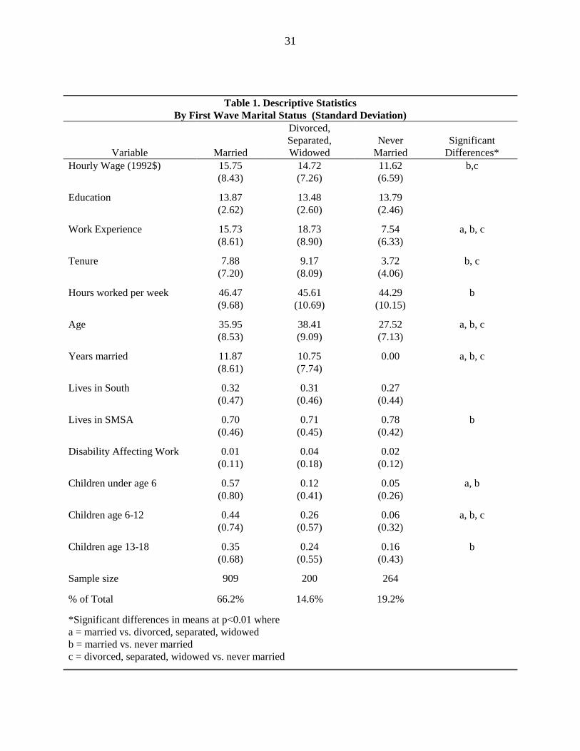
Table 1 provides descriptive statistics for the sample based on data from the first survey,

stratified by marital status as of the first survey date. We consider three marital status categories:

currently married; divorced, separated, or widowed (henceforth previously married); and never-

married. Sixty-six percent of the men are married and 14.6 percent have previously been but are

not currently married. As the values indicate, married men have hourly earnings about 7 percent

higher than previously married men and about 35 percent higher than never-married men.

4 In addition, for eleven of the respondents computed wage differs by more than a factor of five between the first and

second survey. At least one of these wage measures was invariably calculated based on a measure of usual annual or

monthly earnings and is likely incorrect. Panel estimates are especially sensitive to such measurement error hence

these observations are excluded. Also excluded were a handful of observations lacking information on other

variables used in the regression analysis, such as education.

5 Consistent information on union status is unavailable from this survey. The estimated returns to marriage are

unaffected by exclusion of the available measures; hence these measures are excluded from the specifications

presented in this paper.

9

Although there are significant differences by marital status in the means of many of the variables

(indicated in the last column of Table 1), the most substantial differentials are in age, experience,

tenure, and children. The differentials in experience and tenure are important because these

variables are typically found to be important determinants of wages. The role of children is

explored separately in the wage analysis. The lower average wage for never-married men is

certainly due in part to the fact that ever-married men have more experience and tenure than do

never-married men.

Since those changing marital status are the primary force behind the fixed effects estimates,

it is important to examine the frequency of marital status changes within the sample. Within the

almost 6 years between survey periods, 22 percent of the respondents in the panel data sample

changed marital status. Eleven percent of the men married as of the first wave were no longer

married by the second wave, and 45 percent of the men classified as previously married at the

time of the first wave had remarried by the second wave. Of the men who had never been

married as of the first wave, 39 percent were classified as married and another 6 percent as

previously married by the time of the second wave.

The detailed information on home production essential to this study was elicited by asking

respondents to report the time spent by themselves on nine activities: “meal preparation”

(MEALS), “washing dishes and cleaning up after meals” (DISHES), “house cleaning”

(CLEANING), “outdoor and other household maintenance tasks” (OUTDOOR &

MAINTENANCE), “shopping for groceries and other household goods” (SHOPPING),

“washing, ironing and mending” (LAUNDRY), “paying bills and keeping other financial

records” (BILLS), “auto maintenance and repair” (AUTO), and “driving other household

10

members to work, school, or other activities” (DRIVING OTHERS).6 A number of respondents

failed to provide responses to questions about one or more household tasks, particularly during

the first wave of interviews. NSFH personnel indicate that many respondents to this wave left

blanks instead of filling in zeros as the directions requested. Interviewers were instructed to

check for this during the second wave, thus leading to substantially improved response rates.

Some non-responses from the first wave can reasonably be assigned zero values based on

answers to other questions. For instance, driving time is set to zero for those not answering the

question about time spent driving who report that they have not driven a car for over six months.

Other missing responses from the first wave are coded zero if the respondent answered at least

six of the nine questions.7 We consider reported housework time to be unreliable for those who

fail to report housework time in more than three categories at the time of the first survey, and for

those in either survey who report “some” time in an activity rather than a magnitude or who

report an implausible seventy hours or more of housework activity per week. We exclude the

263 respondents with unreliable housework measures from the housework time analyses, but

include them in the wage analyses with all housework measures set to zero and two dummy

variables to indicate which survey contained the unreliable housework measure. Since these

6 The introductory wording for this series of question was: "The questions on this page concern household tasks and

who in your household normally spends time doing those tasks. Write in the APPROXIMATE number of hours per

week that you, your husband or wife, or others in the household normally spend doing the following things. If no

time is spent doing the household task, write in '0'."

7 The activities most often affected by this recoding are OUTDOOR & MAINTENANCE and AUTO. There were

54 cases recoded with one missing housework measure, 22 with two, and 21 with three for the panel based sample

not missing information from the second wave survey. We examine the robustness of the estimates to this imputation

procedure and to other sample selection criteria later.

11

missing data were not entirely random but more likely to arise for married and for disabled men

in the first wave, we perform a variety of sensitivity tests that are discussed later.

As the focus of this paper is upon housework time, it is important to consider the accuracy of

the reported data. Juster and Stafford (1991) provide an excellent discussion of time allocation

studies. They report that survey data like those utilized here tend to overstate true time spent on

most activities. Only in the case of activities that are sporadic in nature such as home repairs do

they recommend use of survey data to supplement diary-based measures. Indeed, a comparison of

diary-based data from the Time Use Survey (TUS) with the NSFH data employed here indicates

substantial differences. Married men working full-time report an average of 11.01 hours of

housework per week in the TUS and 17.86 hours per week in this sample of white, non-

Hispanics from the NSFH. In part the difference may be due to an increase in housework done

by men over time between the TUS survey period of 1975 – 76 and the NSFH survey period of

1987 – 88, but the magnitude of the difference suggests that housework time is likely to be

overstated in the NSFH.8 We investigate in the empirical section whether measurement error

alters the findings of this paper by using, among other variables, the wife’s report of her

husband’s housework time as an instrument for husband’s own report.

Also of some concern is the lack of specific information on childcare activities in the NSFH.

Fortunately, many of the activities associated with children - like additional cleaning, cooking,

and driving - appear to be incorporated in the housework measures reported here. Married men

with children spend over one hour more per week on housework than married men without

children, while married women with children spend over eight hours more per week on

8 We use the NSFH rather than the TUS primarily because the NSFH has substantially more observations. Only

1519 individuals of any age, race, or gender were interviewed for the first wave of the TUS.

12

housework than married women without children. The types of childcare activities least likely to

be included are activities such as playing and reading, which may be more accurately denoted

leisure activities. Nevertheless, to address concerns regarding the measurement of childcare

activities, we estimate wage equations that explicitly control for the number of children in the

household in our sensitivity analysis.

Household Specialization

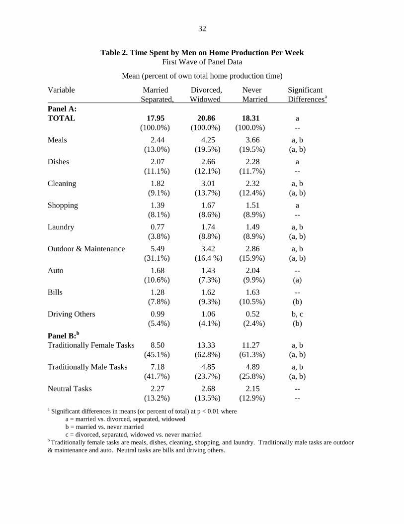
Table 2 provides descriptive statistics by marital status for the housework-related measures.

The measures reported are based on the sample of 1110 observations with valid housework data

from the first wave of our panel data set. Descriptive statistics for the second wave are similar

and are available upon request. The first row indicates that on average married men spend about

the same amount of time on housework, as do never-married men. Both spend on average about

18 hours a week on household activities, while previously married men spend a statistically

significant 3 hours more per week. Further calculations (not reported in the table) show that on

average men with employed wives spend more time on housework than men whose wives are not

employed but the difference is only marginally significant (18.3 versus 16.6 hours: p-value =

0.09).

The statistics in Table 2 indicating that married men spend about the same amount of time

on home production as do never-married men, should not, however, be interpreted to mean that

holding all else constant marital status and housework time are uncorrelated. These

unconditional means do not control for differences in individual circumstances or for differences

in individual preferences that may influence time spent on housework. Some changes in life-

style occur as individuals age and as their assets increase, even in the absence of marital status

13

changes. Alternatively, men who spend more time on housework may be more likely to marry,

but marriage reduces their housework time. Thus, even in the absence of specialization

attributable to marriage, we may expect differences in time spent on household activities

according to individual and household characteristics.

To isolate the effect of marital status on housework time from individual preferences and

unobserved life-cycle factors that are linear with age, we estimate fixed effects, reduced form

housework equations of the form:

(1) itiititit CMSTZHW µγδ +++=

where HWit is time spent on housework by individual i at time t, Z is a vector of observable

characteristics expected to affect time spent on housework, and MST is a vector of indicator

variables for marital status. The term C represents an unobserved individual fixed effect, such as

taste for home production or for domestic comforts. First-difference estimation of this equation

nets out this unobserved individual fixed effect.

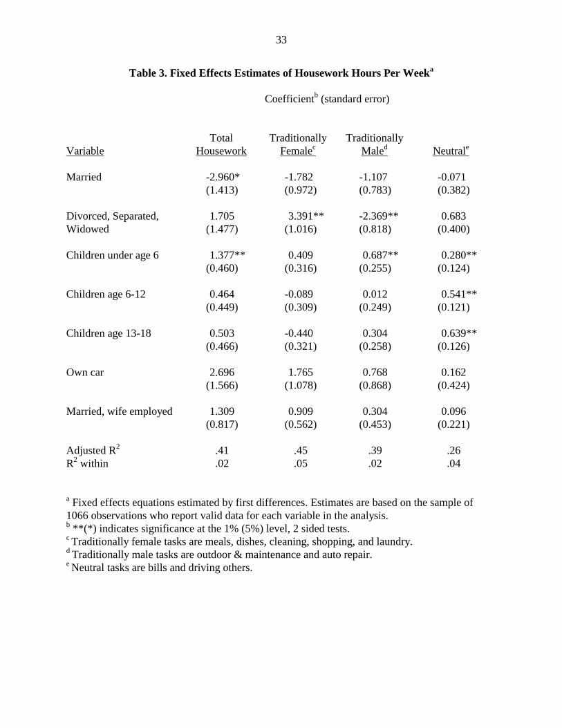
Estimates of housework equations are presented in Table 3. The dependent variable in

Column 1 is total housework time per week. The observable time varying factors for which we

control include marital status, the number of children under age 6, the number of children age 6-

12, the number of children age 13-18, car ownership, and an indicator of wife’s employment

status. Most of the explanatory power is provided by the fixed effects, Ci, which jointly explain

70 percent of the variation in reported housework time. Each additional child under age 6 adds

about 80 minutes per week to housework time. Older children have a much smaller impact that

is not statistically significantly. Buying a car increases housework time by over 2.5 hours per

week, but the effect is significant only at the 10 percent level.

14

Although the raw means of Table 2 reveal little difference in housework time between

married and never-married men, the estimates from Table 3 provide evidence that, conditional on

other factors influencing housework time and net of unobserved individual fixed effects,

marriage can allow men to specialize by decreasing their time on housework. In particular,

conditional on other factors including a fixed individual-specific effect, those men who marry for

the first time and whose wives are not employed report a 3 hour reduction in housework as

compared to those whose marital status is unchanged.9 Wife’s employment status mitigates this

marital effect, with married men whose wives become employed reporting more time spent on

housework, but this spousal employment effect is only marginally significant (p-value = 0.11).

Any time saved during marriage, moreover, ends when that marriage ends. Indeed men whose

marriages end report spending more time on housework than do never-married men with similar

household characteristics, though the difference is not statistically significant.

The results of pooled cross-sectional estimates are fairly similar. Men married to women

who are not employed report spending 2.9 fewer hours per week on housework than do never-

married men (versus 3.0 in fixed effects). Men married to employed women also report spending

fewer hours per week than do never-married men but the differential is smaller (1.0 versus 1.7

hours in fixed effects), and previously married men report spending significantly more time on

housework than do never-married men (3.4 hours versus 1.7 in fixed effects).

9 By reducing time on housework, marriage may allow men to increase their time on market work. If so, the marital

wage differential could be explained by increased investment in job related human capital. In fact, the correlation

between changes in housework time and changes in market hours is a statistically insignificant –0.025 for the sample

that marries between waves.

15

Clearly marital status influences time spent on housework, controlling for various personal

characteristics. However, if the link between marital status and wages depends on the total

amount of time, the relatively small housework time difference between married and never-

married men, regardless of wives’ employment status, suggests that specialization does not

explain the substantial marriage premium in hourly wages observed throughout the literature.

Specialization may, however, explain the premium if different types of housework have different

impacts on wages. Some types of household activities may be more easily postponed or

scheduled so as not to interfere with market activities and some may almost complement market

related activities. If married men are generally less involved in the types that reduce wages, the

observed marriage premium may simply reflect this reduced involvement and could disappear

once adequate controls for home production are added to the wage equation.

Indeed, the allocation of total time among household chores is quite different by marital

status. The descriptive statistics in Table 2 indicate that married men spend a significantly

smaller share of their time on meal preparation, cleaning, and laundry and a significantly larger

share of their household time on outdoor work/home maintenance, than do men who are not

married. It is interesting to note by comparison that previously married men spend more time

than never-married men do on housework, but allocate it similarly.

This differential allocation of housework time can be seen even more clearly when home

production activities are grouped into three activities using a classification method employed by

sociologists (e.g., South and Spitze 1994). One purpose of the classification scheme is to

distinguish among tasks that, within households, are disproportionately performed by either the

husband or the wife, or are performed in nearly equal proportions by husbands and wives. This

classification scheme simultaneously distinguishes between tasks that must be done fairly

16

frequently, often on a daily basis, versus those that can be attended to less often and are easier to

postpone. Thus, meal preparation, dishes, cleaning, shopping, and laundry are categorized as

"traditionally female" type tasks. Auto repair and outdoor/maintenance work are labeled

"traditionally male" type tasks, while bill paying and driving others are "neutral" tasks. Meal

preparation and dishes must be tackled daily, while outdoor work and home maintenance can

vary widely with the season and with household or individual preferences. Outdoor work and

home maintenance can often be delayed, avoided, or contracted out.

Panel B of Table 2 shows the breakdown of housework time using this classification

scheme. Married men spend about 45 percent of their total housework time on traditionally

female tasks, while previously married men spend 63 percent and never-married men 61 percent

of their time. Calculations using our data (not reported in the table) show that within married

households, the gender division of tasks is quite pronounced. By the husbands’ own estimates,

their wives’ share of the total time spent on traditionally female tasks is 76 percent. In contrast,

the wives’ share of traditionally male tasks within the household is 18 percent, while the neutral

tasks are shared more equally, with wives performing 56 percent of the household total. If it is

primarily the daily tasks categorized here as traditionally female that negatively influence

productivity and wages, then married men may earn a wage premium attributable to

specialization as they relinquish tasks in this category.

Estimates examining whether these different categories of housework are affected differently

by marital status are presented in columns 2 - 4 of Table 3. The dependent variable in columns 2

- 4, respectively, is time spent on traditionally female tasks, traditionally male tasks, and neutral

tasks. Marriage has its greatest effect on traditionally female tasks, reducing the time men spend

per week by 1.8 hours (p-value of 0.067). Time spent on traditionally male tasks is also reduced

17

though the impact is not significant, while time spent on neutral tasks is essentially unchanged.

Again the wife's employment status acts to mitigate changes in housework time. Finally, while

men whose marriages have ended report spending about the same amount of time on housework

as never-married men, the allocation is different. Consistent with the unconditional sample

means in Panel B of Table 2, men whose marriages end between interviews spend significantly

more time on traditionally female tasks and less time on traditionally male tasks than do never-

married men.

We also estimated housework equations incorporating a measure of the hours worked by the

wife rather than simply an indicator of her employment status. The total time spent on

housework is significantly affected by wife’s market hours, primarily via its impact on

traditionally female activities. A husband whose wife works 40 hours per week, for example, on

average spends a statistically significant additional 1.8 hours per week on housework, 1.6 of

those hours being spent on traditionally female housework. However, since wife's market hours

were missing substantially more often than wife's employment status, we report in the text the

results with the dummy variable for employment status. Overall, these findings indicate that the

employment status of the wife does provide evidence of specialization as assumed in earlier

studies, though a more direct measure of housework would provide a richer measure.

Household Specialization and the Marriage Wage Premium

To estimate the degree to which the marriage wage premium is attributable to household

specialization, we begin by estimating the marriage wage premium itself using a wage equation

of the following form:

(2) itiititit AMSTXW εγβ +++=ln

18

where ln Wit is the logarithm of the real hourly wage of individual i at time t; X is a vector of

observable individual, human capital, and job characteristics expected to affect the wage; MST is

a vector of marital characteristics including indicator variables for marital status and a quadratic

in years married; and A represents an unobserved individual fixed and time invariant effect, such

as market ability. If men with more ability are more likely to marry, omitting A imparts an

upward bias to the estimate of the return to marriage. If this unobserved characteristic is

genuinely time invariant, fixed effects estimation eliminates the unobserved fixed effect and

provides an unbiased estimate of the return to marital status. A comparison of fixed effects to

cross-sectional estimates provides information on the importance of selection.

We augment equation (2) by including measures of time spent on home production to

examine the impact of specialization on the marriage premium:

(3) itiitititit AHWMSTXW εδγβ ++++=ln

where HW is a vector of home production or specialization measures, measured as either total

time spent on housework or the time spent on various types of housework. This vector also

includes two dummy variables to identify those 263 respondents whose housework measures

have been replaced by zeros because of unreliable values in either of the two waves. This

approach controls for at least some forms of sample selection bias. If it is specialization that

explains the marital wage differential, then including HWit should drive γ to zero.

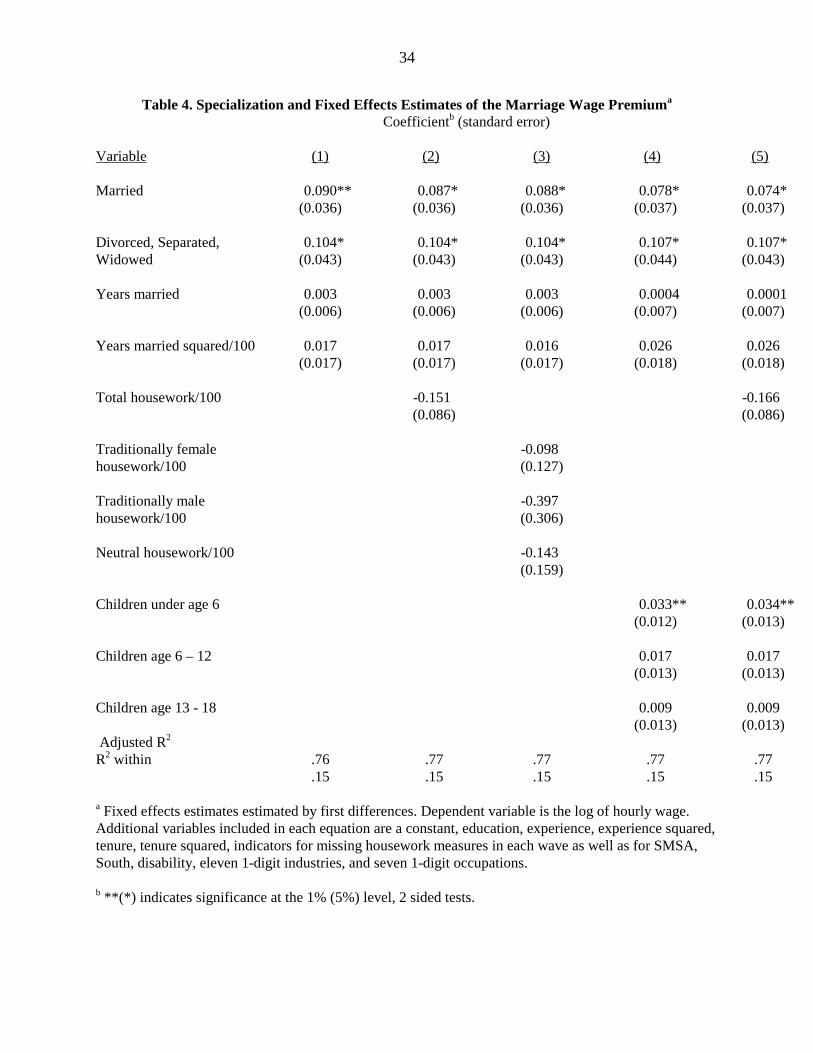
Table 4 presents the key coefficients for wage equations (2) and (3). (Complete results are

available upon request.) In each equation, the vector Xit includes controls for education,

quadratics in work experience and in tenure, and indicators for residence in the South, residence

in an SMSA, a job-related disability, eleven 1-digit industries, and seven 1-digit occupations. In

19

every case, the results indicate that wages increase with education, and with experience and

tenure at a decreasing rate.

The marriage premium is substantial and statistically significant. The coefficients on

married and previously married are 0.090 and 0.104, indicating a wage advantage of 9.4 percent

and 11.0 percent, respectively, relative to men who have never been married. A quadratic in

years married is included in order to permit wages to grow more rapidly during marriage, as

would be the case if men invest more in job related human capital while married. Neither the

coefficient on years married nor the coefficient on its square is individually significant, although

a test of their joint significance yields a p-value of 0.10.

Since tenure, industry and occupation may be affected by marital status, we also estimate

fixed effects models excluding these variables. The results yield slightly smaller coefficient

estimates for both marital status indicators. This suggests that the marital status effect is robust

with respect to any correlation between marital status and work characteristics. (Results available

upon request.)

These fixed effects estimates of the marital wage differential correct for some but not all

marriage selection concerns. Fixed effects estimation should control for unobserved time-

invariant individual-specific characteristics that influence the probability of marriage. Cross-

sectional estimates of the specification in column (1) indicate that married men earn about 11

percent more than do never-married men. The smaller impact of marriage in the fixed effects

estimates (9.4 versus 11.0 percent) provides evidence that selection matters but it explains less

than half of the marriage premium.

Turning to the estimates including housework time in columns 2 and 3, we find in column 2

that housework has a negative effect on wages that is significant at the 7 percent level, with ten

20

additional hours of housework time reducing wages by about 1.7 percent.10 However, inclusion

of this measure has essentially no impact on the magnitude of the marriage premium. The

coefficient on the married indicator variable drops slightly from 0.090 to 0.087. Breaking down

total housework into three categories (traditionally female, traditionally male, neutral) in column

3 yields the same marital wage differential. None of these categories individually has a

significant effect. Further analysis (not reported here) including all nine types of housework

indicates that much of the negative effect of total household tasks on men’s wages appears to be

driven by time spent on meal preparation and, to a lesser extent, on outdoor/maintenance

activities and driving other household members, but once again, the marriage premium declines

by less than five percent.11 Sensitivity tests indicate that these results are robust to a variety of

alternative specifications of the marriage vector.12

In order to address concerns about measurement of child care activities, we re-estimate the

specification reported in column 2 augmenting the wage equation with variables indicating the

10 These results are corroborated by Hersch and Stratton (1997) who find that housework time has a statistically

significant negative effect on wages, especially for married women, and the inclusion of housework time in the wage

equation increases the explained component of the gender wage gap by about 30 percent.

11 The dummy variables for missing housework information are discussed later, in the section devoted to missing

housework data.

12 Among the specifications tested were one without any controls for time married; one with controls for time

married and time separated, divorced, or widowed; and one in which marital status was interacted with time married.

In the latter specification, wages appeared to rise less rapidly during marriage for those whose marriages have since

ended, but the differential was not statistically significant at even the 10 percent level. Also estimated with robust

findings were fixed effects estimates excluding tenure, industry, and occupation and pooled cross-section models.

These results are available upon request.

21

total number of children in each of the three age groups. The marital wage differential shown in

column 4 is clearly smaller, the coefficient having fallen from 0.090 to 0.078. Children of all

ages tend to increase wages, but the effect is only statistically significant for children under the

age of 6. However, controls for housework time continue to have no impact on the marital wage

differential, as indicated by a comparison of columns 4 and 5. The results are similar when

replacing total housework with the three types of housework or with the nine types of housework.

The marital wage differential observed in this study differs somewhat from that observed in

other studies. Korenman and Neumark (1991), for example, find that dummy variables for

marital status have significant coefficients in a fixed effects wage specification that does not

control for marital duration, but that these variables have no significant effect on wages once

controls for marital duration are included. Gray (1997) reports no significant marital wage effect

at all in a fixed effects model using data similar to Korenman and Neumark's but from a later

time period.13 All of the previously cited works on the marital wage differential, however, rely

on samples in which the oldest respondent is only 36 years old. The average age of our sample is

35 in wave 1. Both Korenman and Neumark and Gray control for a quadratic in experience but

not for tenure, possibly because of multicollinearity problems within their young samples. In our

sample, experience and years married are highly correlated. Excluding experience increases the

significance of the marriage duration coefficients but does not change the basic results.

For comparison to earlier studies, we estimated the wage equations restricting the sample to

those under the age of 35 in the first wave (results available upon request). This age restriction

13 Korenman and Neumark use data from the National Longitudinal Survey, Young Men’s Cohort (NLSYM) for the

years 1976, 1978, and 1980. Gray uses NLSYM data for the same years and National Longitudinal Survey of Youth

(NLSY) data for the years 1989, 1991, and 1993.

22

results in substantial multicollinearity between experience, tenure, and years married. Given our

substantially smaller sample size in this age group, multicollinearity problems make the results

including even two of these three variables difficult to analyze. Excluding both years married

and tenure yields a coefficient of 0.03 for married men and of 0.09 for previously married men.

Korenman and Neumark report estimates of 0.06 and 0.04 using the same specification. These

results are not dissimilar, particularly given the high standard errors associated with each. Most

importantly, inclusion of time spent on housework in a wage equation for this young sample does

not affect the estimated marriage premium either.

We examined three additional hypotheses regarding the effect of housework upon wages.

First, if time spent on housework today influences the amount of on-the-job investment today and

hence wages tomorrow, then controls for the complete history of housework time may influence

wages or wage growth. As a partial control, we include the only available earlier measure,

housework at the time of the first survey, in the wage difference estimates. Introduction of this

variable indicates that those spending more time on traditionally female tasks in the first wave

have slower wage growth between waves. However, inclusion of the level of housework time in

the first wave in any form leaves unchanged the magnitude of the marital wage differential.

Second, the effect of housework time on wage growth may differ by marital status. Indeed, there

is some indication that the effect of housework is larger for those previously married, but the

terms interacting housework time with marital status are not statistically significant either

individually or jointly. Finally, the wage-enhancing effects of specialization may be due to the

housework time spent by the wife rather than that spent by the husband. Wage equations

including total or disaggregated measures of wives' housework time indicate that wives'

housework time is not a statistically significant determinant of men’s wages.

23

In summary, the marital wage differential is remarkably persistent. It remains even after

controlling for selection by allowing for fixed individual-specific effects. Although there are

substantial differences by marital status in conditional hours of housework, the marriage

premium is unaffected by the inclusion of housework time in the wage equation. If marriage

makes men more productive, it does not appear to do so because of specialization within the

household.

Missing housework data

As discussed earlier, data on housework time from the first survey are missing far more

often than data from the second survey and our results could be attributed to the peculiarities of

our housework data. We employed an imputation procedure to assign zeros to missing

housework time in the first survey for those individuals who provided valid information on at

least six of the nine types of housework, and included dummy variables to identify the remaining

observations with missing or invalid values in the wage analysis. The coefficient on the dummy

variable indicating missing housework data from wave two is consistently statistically

insignificant, suggesting that missing housework data from this wave is uncorrelated with wages.

The coefficient on the dummy variable indicating missing housework data from the first wave,

however, is consistently positive, of the same magnitude in all wage equations, and statistically

significant at about the 7 percent level. Since our first difference estimates subtract period 1

values from period 2 values, the positive coefficient on the dummy variable implies that those

failing to report housework in wave one had significantly lower wage growth between

interviews. To check the sensitivity of the wage equation estimates to the imputation procedure,

we re-estimated the wage equations allowing between zero and five missing values to be

24

imputed. The results were not sensitive to this assignment. We also restricted the analysis to

only those observations that did not require any imputation of housework time and obtained

similar results.

Endogeneity and Measurement Error

While sample selection and data definition concerns regarding housework time do not

appear to influence the basic results reported here, there are two other possible sources of bias

relating to housework. First, housework time may be determined endogenously with the wage.

Endogeneity driven by individual-specific time invariant characteristics is remedied by the fixed

effects estimation technique employed above. However, fixed effects estimation will not

eliminate other sources of endogeneity. For instance, if men with faster wage growth do less

housework, the fixed effects estimates will themselves be biased.

Second, housework time may be measured with error. One possible form measurement error

could take is that respondents systematically over- or understate their housework time by a

constant amount in each wave. This source of measurement error would be eliminated in the

fixed effect estimates. But random measurement error will bias the estimated coefficient on

housework toward zero, and this bias is likely to be exacerbated in panel data estimates.14

In the presence of either endogeneity bias or measurement error, the coefficient on

housework, and on any other variable correlated with housework (such as marital status), will be

14 The primary concern in other studies examining the marriage premium has been the endogeneity of marriage. As

discussed earlier, to the extent that men who marry are more productive, the marital wage effect will be biased

upward in cross-sectional estimates. Fixed effects estimation removes this type of endogeneity bias, but not, for

example, selection based on wage growth. As mentioned earlier, neither Korenman and Neumark (1991) nor Gray

(1997) find evidence of such selection.

25

biased. A possible solution to both problems is instrumental variables estimation. The data set

provides a wide array of plausible instruments for housework time. Since many of these

potential instruments are constant over the panel and since the explanatory power of the time

varying covariates in the panel data housework equations is low, we use only the first wave

cross-section reporting valid data on housework so that we can include a broader set of

instruments. In particular, we use as instruments car ownership; 8 measures of the number of

other adults in the household: distinguishing between male and female children age 19 and older,

male and female parents, male and female other relatives, and male and female nonrelatives; the

respondents’ parents’ education; 3 variables indicating whether the respondent’s mother worked

outside the home when the respondent was under age 6, age 6 – 11, or age 12– 17; and 5 missing

value indicators for these latter 5 variables. (Results available upon request.)

A Hausman test fails to reject the hypothesis that the OLS estimates are consistent,

indicating that neither endogeneity nor measurement error are substantial problems. Coefficient

estimates for the housework measure are statistically insignificant in both OLS and IV estimates.

A test of the power of the instruments not also in the wage equation indicates that these

instruments are jointly significant. In addition, a Lagrange Multiplier test confirms that the

instruments do not belong themselves in the wage equation; the exclusion restrictions are valid15.

Varying the instrument set to test the exogeneity of the instruments with respect to wages yields

similar results: the instruments appear to be exogenous.

15 The value of the Hausman test statistic is 1.72. This statistic is distributed chi-squared with 30 degrees of

freedom and soundly fails to reject the null hypothesis that housework is exogenous. The test statistic for the power

of the instruments is 1.91. It is distributed F with 19 and 1133 degrees of freedom. The Lagrange multiplier test

statistic, distributed chi-squared with 19 degrees of freedom, is 16.2.

26

Although technically these instruments are valid, the overall fit of the housework equation is

weak, with an adjusted R2 of 0.03. Our failure to find evidence of endogeneity or of

measurement error may be due to our weak instrument set. At least for the case of measurement

error, we can test this hypothesis on a subset of observations by introducing what is certainly a

powerful instrument: the wife’s report of her husband’s housework time. This instrument is

necessarily available only for the subsample of married men whose wives provided such a report.

Within this sample of 465 married men, inclusion of wife’s report increases the adjusted R2 of

the housework equation from 0.011 to 0.086; the wife's report is clearly highly correlated with

the husband's report, making it a good instrument. A Lagrange Multiplier test confirms that the

exclusion restrictions are valid; the wife’s report does not itself belong in the wage equation. For

this sample of married men, the coefficient on housework in the IV specification is –0.27 (p-

value = 0.56), while the corresponding coefficient in OLS estimates is –0.07 (p-value = 0.68).

The difference in magnitude provides some evidence of measurement error, but neither estimate

provides statistical evidence strong enough to warrant much attention. The IV and OLS

coefficients in the wage equation are not statistically significantly different: a Hausman test fails

to reject the hypothesis that housework is exogenous with respect to wages. As this sample has

been restricted to married men, no estimate of the marital wage differential can be obtained using

these data, but these findings suggest that measurement error is not a serious problem and that

our earlier failure to reject exogeneity is not simply due to weak instruments.

Conclusion

From the perspective of economists, an important benefit of marriage is that it allows

spouses to specialize in either market or home production, creating a bigger “pie” to be shared by

27

all members of the household. Historically, husbands have been more likely to specialize in the

market. The commonly observed marriage premium for men is frequently attributed to either

selection of more productive men into marriage or to enhanced productivity resulting from the

specialization possible within a joint household. In this paper, we examine the specialization

hypothesis. We present evidence on the amount of time spent in home production by men

according to their marital status. We then examine the impact that controlling for home

production activities and selection has on the estimated marriage premium.

Our results indicate that the marriage premium is not primarily due to the selection of more

productive men into marriage. Marriage does seem to make men more productive in the market.

However, this enhanced productivity does not seem to result from household specialization.

There is little difference by marital status in the total amount of time spent by men on home

production, although there are differences in the type of home production activities. Not

surprisingly, married men spend less time on tasks such as cooking and cleaning than those not

married. With little difference in the total time spent on housework, the only way that

specialization can explain the premium is if different types of housework have different impacts

on wages. While we find evidence that own time spent on home production negatively affects

wages; controlling for housework time does not have a substantial impact on the marriage

premium.

If specialization does not make married men more productive, what could explain the

marriage premium? Married men may get preferential treatment from employers, such as more

training or promotions. Or men may become better workers because of the stability induced by

marriage. These explanations cannot be modeled using an individual fixed effect, since they

suggest an actual change in behavior resulting from marriage or the decision to marry. If neither

28

selection nor specialization explains the differential, then more attention should be paid to

alternative explanations such as these.

29

ReferencesBecker, Gary S. 1991. A Treatise on the Family. Enl. ed. Cambridge, Mass.: HarvardUniversity Press.

Becker, Gary S. 1985. "Human Capital, Effort, and the Sexual Division of Labor." Journal ofLabor Economics, Vol. 3, No. 1, part 2 (January), pp. S33-S58.

Cornwell, Christopher, and Peter Rupert. 1997. “Unobserved Individual Effects, Marriage andthe Earnings of Young Men.” Economic Inquiry, Vol. 35, No. 2 (April), pp. 285-94.

Daniel, Kermit. 1991. “Does Marriage Make Men More Productive?” Unpublished paper,University of Chicago.

Gray, Jeffrey S. 1997. “The Fall in Men’s Return to Marriage: Declining Productivity Effects orChanging Selection?” Journal of Human Resources, Vol. 32, No. 3 (Summer), pp. 481-504.

Hersch, Joni. 1991. “Male-Female Differences in Hourly Wages: The Role of Human Capital,Working Conditions, and Housework.” Industrial and Labor Relations Review, Vol. 44, No. 4(July), pp. 746-59.

Hersch, Joni, and Leslie S. Stratton. 1997. “Housework, Fixed Effects, and Wages of MarriedWorkers.” Journal of Human Resources, Vol. 32, No. 2 (Spring), pp. 285 – 307.

Juster, F. Thomas, and Frank P. Stafford. 1991. "The Allocation of Time: Empirical Findings,Behavioral Models, and Problems of Measurement." Journal of Economic Literature, Vol. 29,No. 2 (June), pp. 471-522.

Kenny, Lawrence W. 1983. “The Accumulation of Human Capital During Marriage by Males.”Economic Inquiry, Vol. 21, No. 2 (April), pp. 223- 31.

Korenman, Sanders, and David Neumark. 1991. "Does Marriage Really Make Men MoreProductive?" Journal of Human Resources, Vol. 26, No. 2 (Spring), pp. 282-307.

Loh, Eng Seng. 1996. "Productivity Differences and the Marriage Wage Premium for WhiteMales." Journal of Human Resources, Vol. 31, No. 3 (Summer), pp. 566-89.

Nakosteen, Robert A., and Michael A. Zimmer. 1986. “Marital Status and Earnings of YoungMen.” Journal of Human Resources, Vol. 22, No. 2 (Spring), pp. 248-68.

Reed, W. Robert, and Kathleen Harford. 1989. "The Marriage Premium and CompensatingWage Differentials." Journal of Population Economics, Vol. 2, No. 4, pp. 237-265.

South, Scott J., and Glenna Spitze. 1994. "Housework in Marital and Nonmarital Households."American Sociological Review, Vol. 59, No. 3 (June), pp. 327-47.

30

Sweet, James A., and Larry L. Bumpass. 1996. The National Survey of Families andHouseholds - Waves 1 and 2: Data Description and Documentation. Center for Demography andEcology, University of Wisconsin-Madison (http://ssc.wisc.edu/nsfh/home.htm).

Sweet, James, Larry Bumpass, and Vaughn Call. 1988. "The Design and Content of TheNational Survey of Families and Households." Center for Demography and Ecology, Universityof Wisconsin-Madison, NSFH Working Paper #1.

31

Table 1. Descriptive StatisticsBy First Wave Marital Status (Standard Deviation)

Variable Married

Divorced,Separated,Widowed

NeverMarried

SignificantDifferences*

Hourly Wage (1992$) 15.75 14.72 11.62 b,c(8.43) (7.26) (6.59)

Education 13.87 13.48 13.79(2.62) (2.60) (2.46)

Work Experience 15.73 18.73 7.54 a, b, c(8.61) (8.90) (6.33)

Tenure 7.88 9.17 3.72 b, c(7.20) (8.09) (4.06)

Hours worked per week 46.47 45.61 44.29 b(9.68) (10.69) (10.15)

Age 35.95 38.41 27.52 a, b, c(8.53) (9.09) (7.13)

Years married 11.87 10.75 0.00 a, b, c(8.61) (7.74)

Lives in South 0.32 0.31 0.27(0.47) (0.46) (0.44)

Lives in SMSA 0.70 0.71 0.78 b(0.46) (0.45) (0.42)

Disability Affecting Work 0.01 0.04 0.02(0.11) (0.18) (0.12)

Children under age 6 0.57 0.12 0.05 a, b(0.80) (0.41) (0.26)

Children age 6-12 0.44 0.26 0.06 a, b, c(0.74) (0.57) (0.32)

Children age 13-18 0.35 0.24 0.16 b(0.68) (0.55) (0.43)

Sample size 909 200 264

% of Total 66.2% 14.6% 19.2%

*Significant differences in means at p<0.01 wherea = married vs. divorced, separated, widowedb = married vs. never marriedc = divorced, separated, widowed vs. never married

32

Table 2. Time Spent by Men on Home Production Per WeekFirst Wave of Panel Data

Mean (percent of own total home production time)

Variable Married Divorced, Never SignificantSeparated, Widowed Married Differencesa

Panel A:TOTAL 17.95 20.86 18.31 a

(100.0%) (100.0%) (100.0%) --

Meals 2.44 4.25 3.66 a, b(13.0%) (19.5%) (19.5%) (a, b)

Dishes 2.07 2.66 2.28 a(11.1%) (12.1%) (11.7%) --

Cleaning 1.82 3.01 2.32 a, b(9.1%) (13.7%) (12.4%) (a, b)

Shopping 1.39 1.67 1.51 a(8.1%) (8.6%) (8.9%) --

Laundry 0.77 1.74 1.49 a, b(3.8%) (8.8%) (8.9%) (a, b)

Outdoor & Maintenance 5.49 3.42 2.86 a, b(31.1%) (16.4 %) (15.9%) (a, b)

Auto 1.68 1.43 2.04 --(10.6%) (7.3%) (9.9%) (a)

Bills 1.28 1.62 1.63 --(7.8%) (9.3%) (10.5%) (b)

Driving Others 0.99 1.06 0.52 b, c(5.4%) (4.1%) (2.4%) (b)

Panel B:b

Traditionally Female Tasks 8.50 13.33 11.27 a, b(45.1%) (62.8%) (61.3%) (a, b)

Traditionally Male Tasks 7.18 4.85 4.89 a, b(41.7%) (23.7%) (25.8%) (a, b)

Neutral Tasks 2.27 2.68 2.15 --(13.2%) (13.5%) (12.9%) --

a Significant differences in means (or percent of total) at p < 0.01 wherea = married vs. divorced, separated, widowedb = married vs. never marriedc = divorced, separated, widowed vs. never married

b Traditionally female tasks are meals, dishes, cleaning, shopping, and laundry. Traditionally male tasks are outdoor& maintenance and auto. Neutral tasks are bills and driving others.

33

Table 3. Fixed Effects Estimates of Housework Hours Per Weeka

Coefficientb (standard error)

VariableTotal

HouseworkTraditionally

FemalecTraditionally

Maled Neutrale

Married

Divorced, Separated,Widowed

Children under age 6

Children age 6-12

Children age 13-18

Own car

Married, wife employed

Adjusted R2

R2 within

-2.960*(1.413)

1.705(1.477)

1.377**(0.460)

0.464(0.449)

0.503(0.466)

2.696(1.566)

1.309(0.817)

.41

.02

-1.782(0.972)

3.391**(1.016)

0.409(0.316)

-0.089(0.309)

-0.440(0.321)

1.765(1.078)

0.909(0.562)

.45

.05

-1.107(0.783)

-2.369**(0.818)

0.687**(0.255)

0.012(0.249)

0.304(0.258)

0.768(0.868)

0.304(0.453)

.39

.02

-0.071(0.382)

0.683(0.400)

0.280**(0.124)

0.541**(0.121)

0.639**(0.126)

0.162(0.424)

0.096(0.221)

.26

.04

a Fixed effects equations estimated by first differences. Estimates are based on the sample of1066 observations who report valid data for each variable in the analysis.b **(*) indicates significance at the 1% (5%) level, 2 sided tests.c Traditionally female tasks are meals, dishes, cleaning, shopping, and laundry.d Traditionally male tasks are outdoor & maintenance and auto repair.e Neutral tasks are bills and driving others.

34

Table 4. Specialization and Fixed Effects Estimates of the Marriage Wage Premiuma

Coefficientb (standard error)

Variable (1) (2) (3) (4) (5)

Married

Divorced, Separated,Widowed

Years married

Years married squared/100

Total housework/100

Traditionally femalehousework/100

Traditionally malehousework/100

Neutral housework/100

Children under age 6

Children age 6 – 12

Children age 13 - 18

Adjusted R2

R2 within

0.090**(0.036)

0.104*(0.043)

0.003(0.006)

0.017(0.017)

.76

.15

0.087*(0.036)

0.104*(0.043)

0.003(0.006)

0.017(0.017)

-0.151(0.086)

.77

.15

0.088*(0.036)

0.104*(0.043)

0.003(0.006)

0.016(0.017)

-0.098(0.127)

-0.397(0.306)

-0.143(0.159)

.77

.15

0.078*(0.037)

0.107*(0.044)

0.0004(0.007)

0.026(0.018)

0.033**(0.012)

0.017(0.013)

0.009(0.013)

.77

.15

0.074*(0.037)

0.107*(0.043)

0.0001(0.007)

0.026(0.018)

-0.166(0.086)

0.034**(0.013)

0.017(0.013)

0.009(0.013)

.77

.15

a Fixed effects estimates estimated by first differences. Dependent variable is the log of hourly wage.Additional variables included in each equation are a constant, education, experience, experience squared,tenure, tenure squared, indicators for missing housework measures in each wave as well as for SMSA,South, disability, eleven 1-digit industries, and seven 1-digit occupations.

b **(*) indicates significance at the 1% (5%) level, 2 sided tests.