ISSN 1045-6333

HARVARD JOHN M. OLIN CENTER FOR LAW, ECONOMICS, AND BUSINESS

AGE VARIATIONS IN WORKERS’ VALUE OF A STATISTICAL LIFE

Joseph E. Aldy W. Kip Viscusi

Discussion Paper No. 468

03/2004

Harvard Law School Cambridge, MA 02138

This paper can be downloaded without charge from:

The Harvard John M. Olin Discussion Paper Series: http://www.law.harvard.edu/programs/olin_center/

JEL Codes: J17, I12

Age Variations in Workers’ Value of Statistical Life

Joseph E. Aldy and W. Kip Viscusi *

Abstract

This paper develops a life-cycle model in which workers choose both consumption levels

and job fatality risks, implying that the effect of age on the value of life is ambiguous. The

empirical analysis of this relationship uses novel, age-dependent fatal and nonfatal risk variables.

Workers’ value of statistical life exhibits an inverted U-shaped relationship over workers’ life

cycle based on hedonic wage model estimates, age-specific hedonic wage estimates, and a

minimum distance estimator. The value of statistical life for a 60-year old ranges from $2.5

million to $3.0 million – less than half the value for 30 to 40-year olds.

Keywords: value of life, job risks, hedonic wage regression, VSLY

* Aldy: Department of Economics, Littauer Center, Harvard University, Cambridge, MA 02138 (e-mail: aldy@fas.harvard.edu); Viscusi: Cogan Professor of Law and Economics, Harvard Law School, Hauser Hall 302, Cambridge, MA 02138 (e-mail: kip@law.harvard.edu). Aldy’s research is supported by the U.S. Environmental Protection Agency STAR Fellowship program and the Switzer Environmental Fellowship program. Viscusi’s research is supported by the Harvard Olin Center for Law, Economics, and Business. The authors express gratitude to the U.S. Bureau of Labor Statistics for permission to use the CFOI fatality data. Neither the BLS nor any other government agency bears any responsibility for the risk measures calculated or the results in this paper. Antoine Bommier, David Cutler, Bryan Graham, Seamus Smyth, and Jim Ziliak provided very constructive comments on an earlier draft and we thank participants of the Harvard Environmental Economics and Policy Seminar for their comments.

Age Variations in Workers’ Value of Statistical Life

Joseph E. Aldy and W. Kip Viscusi

© 2004 Joseph E. Aldy and W. Kip Viscusi. All rights reserved.

A strident controversy with respect to the value of life has been whether the benefit of

reducing risks to the old are less than for younger age groups. In particular, should there be a so-

called “senior discount” when assessing the value of reduced risks to life? This question has

drawn the attention of policymakers in a number of countries. In 2000, Canada employed a

value of statistical life (VSL) for the over-65 population that is 25 percent lower than the VSL

for the under-65 population (Hara and Associates 2000). In 2001, the European Commission

recommended that member countries use a VSL that declines with age (European Commission

2001). In 2003, the U.S. Environmental Protection Agency (EPA), which has traditionally

employed a constant value of a statistical life to monetize mortality risk reductions irrespective

of the age of the affected population, conducted analyses of the Clear Skies initiative that

included a “senior discount.”1 This effort to apply such a discount in its Clear Skies initiative

analyses generated a political firestorm and ultimately led to abandonment of any age

adjustments in benefit values assigned by the Agency.2

1 In the “senior discount” analyses, the EPA provided two alternatives to account for age. One

approach was based on a standard value of a statistical life-year approach that explicitly accounts

for life expectancy. The second approach assumed that individuals over age 70 had a value of

statistical life equal to 63 percent of the value for those under 70.

2 For a sense of the political reaction and EPA’s decision to discontinue the use of an age-based

value of statistical life, refer to “EPA Drops Age-Based Cost Studies,” New York Times, May 8,

1

Intuitively one might expect that older individuals may value reducing risks to their lives

less because they have shorter remaining life expectancy. The commodity they are buying

through risk reduction efforts is less than for younger people. Carrying this logic to its extreme,

the value of a statistical life (VSL) would peak at birth and decline steadily thereafter. For

models in which consumption is constant over the life cycle, Jones-Lee (1976, 1989) first

showed that the VSL should decrease with age. Whether consumption will in fact be constant

over time depends critically on the presence of perfect capital and insurance markets.

Numerous theoretical studies have shown that the age variation in VSL becomes more

complex once changes in consumption over time are introduced into the analysis. Changes in

consumption levels and wealth over the life cycle influence risk-money tradeoffs in a complex

manner. The recent study by Johansson (2002) concluded that the theoretical relationship

between the VSL and age is ambiguous and could be positive, negative, or zero. Often

theoretical studies, however, have imposed additional structure on the analysis, implying that

there is either an inverted U-shaped relationship between the value of statistical life and age or

that VSL decreases with age.

Numerical simulations likewise have suggested that the relationship between VSL and

age is either negative or characterized by an inverted-U shape. The simulations by Shepard and

Zeckhauser (1984) show a steadily declining value of life if there are perfect annuity and

insurance markets, while there is an inverted-U VSL-age relationship in an economy with no

borrowing or insurance. Under illustrative restrictive assumptions, Johansson (1996) also finds

2003; “EPA to Stop ‘Death Discount’ to Value New Regulations,” Wall Street Journal, May 8,

2003; and “Under Fire, EPA Drops the ‘Senior Death Discount,’” Washington Post, May 13,

2003.

2

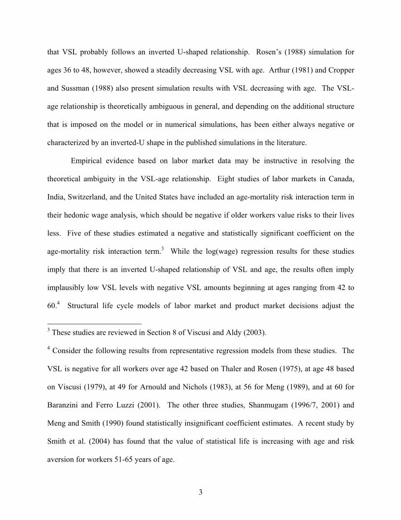
that VSL probably follows an inverted U-shaped relationship. Rosen’s (1988) simulation for

ages 36 to 48, however, showed a steadily decreasing VSL with age. Arthur (1981) and Cropper

and Sussman (1988) also present simulation results with VSL decreasing with age. The VSL-

age relationship is theoretically ambiguous in general, and depending on the additional structure

that is imposed on the model or in numerical simulations, has been either always negative or

characterized by an inverted-U shape in the published simulations in the literature.

Empirical evidence based on labor market data may be instructive in resolving the

theoretical ambiguity in the VSL-age relationship. Eight studies of labor markets in Canada,

India, Switzerland, and the United States have included an age-mortality risk interaction term in

their hedonic wage analysis, which should be negative if older workers value risks to their lives

less. Five of these studies estimated a negative and statistically significant coefficient on the

age-mortality risk interaction term.3 While the log(wage) regression results for these studies

imply that there is an inverted U-shaped relationship of VSL and age, the results often imply

implausibly low VSL levels with negative VSL amounts beginning at ages ranging from 42 to

60.4 Structural life cycle models of labor market and product market decisions adjust the

3 These studies are reviewed in Section 8 of Viscusi and Aldy (2003).

4 Consider the following results from representative regression models from these studies. The

VSL is negative for all workers over age 42 based on Thaler and Rosen (1975), at age 48 based

on Viscusi (1979), at 49 for Arnould and Nichols (1983), at 56 for Meng (1989), and at 60 for

Baranzini and Ferro Luzzi (2001). The other three studies, Shanmugam (1996/7, 2001) and

Meng and Smith (1990) found statistically insignificant coefficient estimates. A recent study by

Smith et al. (2004) has found that the value of statistical life is increasing with age and risk

aversion for workers 51-65 years of age.

3

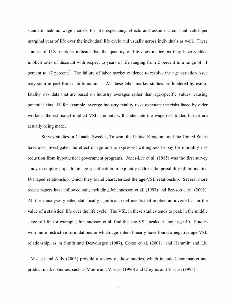
standard hedonic wage models for life expectancy effects and assume a constant value per

marginal year of life over the individual life cycle and usually across individuals as well. These

studies of U.S. markets indicate that the quantity of life does matter, as they have yielded

implicit rates of discount with respect to years of life ranging from 2 percent to a range of 11

percent to 17 percent.5 The failure of labor market evidence to resolve the age variation issue

may stem in part from data limitations. All these labor market studies are hindered by use of

fatality risk data that are based on industry averages rather than age-specific values, causing

potential bias. If, for example, average industry fatality risks overstate the risks faced by older

workers, the estimated implied VSL amounts will understate the wage-risk tradeoffs that are

actually being made.

Survey studies in Canada, Sweden, Taiwan, the United Kingdom, and the United States

have also investigated the effect of age on the expressed willingness to pay for mortality risk

reduction from hypothetical government programs. Jones-Lee et al. (1985) was the first survey

study to employ a quadratic age specification to explicitly address the possibility of an inverted

U-shaped relationship, which they found characterized the age-VSL relationship. Several more

recent papers have followed suit, including Johannesson et al. (1997) and Persson et al. (2001).

All these analyses yielded statistically significant coefficients that implied an inverted-U for the

value of a statistical life over the life cycle. The VSL in these studies tends to peak in the middle

stage of life; for example, Johannesson et al. find that the VSL peaks at about age 40. Studies

with more restrictive formulations in which age enters linearly have found a negative age-VSL

relationship, as in Smith and Desvousges (1987), Corso et al. (2001), and Hammitt and Liu

5 Viscusi and Aldy (2003) provide a review of those studies, which include labor market and

product market studies, such as Moore and Viscusi (1990) and Dreyfus and Viscusi (1995).

4

(2004). Finally, Krupnick et al. (2002) use age group indicator variables and find that VSL is

fairly flat until age 70, for which it is lower. 6

This paper extends the previous literature in several respects. Because our focus is on

risky labor market decisions, we incorporate job risk decisions into a life-cycle consumption

model in Section I, deriving an expression for VSL in this context. In Section II, we develop the

critical input to our empirical analysis – the first age-dependent measure of fatality risk and

injury risk to be used in a hedonic labor market analysis. In Section III we develop several sets

of empirical estimates of the age-VSL relationship: conventional hedonic wage equations, wage

equation estimates for specific age groups, a minimum distance estimator, and regressions with

age-mortality risk interactions that all indicate similar variations in VSL over the life cycle. In

6 Their finding that a 70-year old’s willingness-to-pay (WTP) is about one-third less than the

WTP of those aged 50 to 70 years was a key input in the Environmental Protection Agency’s

recent analysis of the Clear Skies initiative. Two important caveats merit attention. First, as the

authors note, the intercept in the WTP bid regression model, which represents the age effect of

the ≥70-years old age group on WTP, is not statistically significant, although the age group

indicator variable coefficients are all significant for age groups 40-49, 50-59, and 60-69. Thus,

the estimate of the ≥70-years old age group VSL is based on a rather imprecise estimate, as is the

comparison between the <70-years and ≥70-years populations. Second, the age group indicator

variable coefficients imply an inverted-U for VSL over the life cycle. The authors indicate (in

note 22) that with a more stringent data cleaning criterion, they estimate quadratic age regression

specifications that yield an inverted-U with statistically significant coefficient estimates on the

age and age2 variables. Note that while other studies’ sample screens include all adult-aged

individuals, the Krupnick et al. study focuses on individuals 40 to 75 years of age.

5

all of these empirical approaches, the VSL rises and then falls over the life cycle, with a peak in

the 30s, and a subsequent decline so that the VSL for workers in their early 60s have values of

about $2.5-$3 million.7 In Section IV, we calculate age-specific values of statistical life-years

(VSLY) from our age-VSL profiles and find that after VSLYs peak at approximately the same

age as VSLs peak, they decline monotonically with age. Section V concludes the paper.

I. Wage-Risk Tradeoffs over the Life Cycle

To motivate the empirical work, we provide a simple model of wage-risk tradeoffs in a

one-period framework and a life-cycle setting. The implications of these simple models are not

unambiguous with respect to the relationship between age and the VSL, although they do

indicate variations in VSL by age. The life-cycle model can illustrate the influences that can

generate an inverted U-shaped relationship between VSL and age.

As a starting point, and to clearly illustrate the implications of the life-cycle model on the

wage-risk tradeoff estimated in the subsequent empirical work, we provide a one-period model

involving the choice of the riskiness of one’s job.8 Assume in the one-period model that only

two states exist: alive and dead. We normalize the utility of the dead state to zero so that any

bequests have some fixed value. The probability of dying on the job in the period is denoted by

p . In this case, the worker’s problem is to choose consumption and job fatality risk to

maximize expected utility:

7 All VSL estimates are presented in 1996 dollars in this paper. All VSL estimates should be

increased 14.7 percent to convert them to 2002 dollars, based on the CPI-U deflator.

8 See Viscusi (1979), Rosen (1988), and Viscusi and Aldy (2003), among many others, for

details on such one-period models.

6

(1) )()1(max,

cupEUpc

−= ,

subject to

(2) )( pwkc += ,

where

p represents the probability of dying on the job,

)(cu represents the utility of consumption, , and c 0)( ≥′ cu , 0)( ≤′′ cu ,

k represents (initial) assets, and

w represents labor.

Solving for the optimal consumption and job risk yields this familiar expression for the

wage-risk tradeoff:

(3) c

p upuw

)1( −= ,

where

pw represents the derivative of the wage with respect to mortality risk ( p ), and

cu represents the derivative of utility with respect to consumption ( ). c

The value of is the VSL, or the change in the worker’s wage with respect to

occupational mortality risk. The VSL is given by the utility of consumption divided by the

expected marginal utility of consumption. Because a fatal job accident leads to the loss of this

period’s utility as well as all future utility, one would expect there to be an analog of this result

for life-cycle models. The standard approach in the life-cycle VSL literature employs a time-

separable utility function in one consumption good, integrated over the life-cycle subject to a

discount function and a survival function, as in Shepard and Zeckhauser (1984), Rosen (1988),

Johansson (1996, 2002), and Johannesson et al. (1997). These analyses modified the standard

pw

7

life-cycle model to reflect the expected utility of the rest of an individual’s life conditional on the

individual’s current age. We extend the life-cycle approach to explicitly account for the

influence of job fatality risk on the survival function and the worker’s wage. Expected

remaining lifetime utility can then be characterized by:

(4) , ∫∞

−=τ

τστ dtetpttcuEU rt)](,;[)]([)(

subject to

(5a) , )()()](,[)()( tftctptwtrktk +−+=&

(5b) , 0)( ≥tk

and

(5c) , 0)(lim =−

∞→

rt

tetk

where

rte − represents the discount function,

)](,;[ tpt τσ represents the survival function, i.e., the probability of surviving to age t,

given that the individual has reached age τ ,9

r represents the return on assets, and

)(tf represents the net amount received through an actuarially fair annuity represented

by the condition:

0)()](,0;[0

=∫∞

− dttftpte rtσ .

9 This expression of the survival function follows Johansson (1996):

)(/)](;[)](,;[ τσστσ tpttpt = .

8

All other terms are simply their period t analogs to the single-period case.10

The worker’s expected utility is represented in (4) as the sum of period utilities weighted

by a discount factor and the probability that the worker will survive to that period conditional on

the worker’s current age. The worker maximizes this expected utility expression subject to the

constraints: (5a) represents the dynamic budget constraint and it allows for the worker’s assets to

change over time based on capital income ( ), labor income ( ), consumption

( ) ), and net annuity receipts ( ); (5b) provides a no debt condition; and (5c) is the

standard no Ponzi game condition. The actuarially fair annuity envisioned here is similar to that

in Shepard and Zeckhauser’s (1984) perfect markets case, and the annuity allows for the worker

to borrow against human capital during early years of life to provide for consumption smoothing.

)(trk )](,[ tptw

(tc )(tf

The distinctive feature of our formulation is that wages for risky jobs enter the analysis,

and the level of job fatality risk chosen by the worker is a choice variable in the model, as is the

level of consumption in each period. Previous studies instead have focused simply on the life-

cycle consumption choice without embedding in the model a compensating wage differential

framework.

The present value Hamiltonian for this problem, conditional on having lived to age τ, is

given by:

(6) [ ])()()](,[)()()](,;[)]([)( tftctptwtrktetpttcutH rt +−++= − λτσ

10 To simplify notation, we have followed Shepard and Zeckhauser and assumed that the rate of

time preference in the discount function is equal to the rate of return on assets, and that this rate

is time-invariant. Allowing for the rate of time preference to differ from the return on assets

would not substantively impact the primary conclusion of this analysis that the age-VSL

relationship is ambiguous.

9

where )(tλ represents the present value costate variable. The first order conditions for the

Hamiltonian are:

(7) 0=−=∂∂ − λσ rt

c eucH ,11

(8) 0=+=∂∂ −

prt

p weupH λσ ,

and

(9) λλλ rkH

−=→=∂∂

− && .

Substituting equation (7) into equation (8) and solving for yields: pw

(10) c

p

p

u

tcuw⎟⎠⎞

⎜⎝⎛

−=

σσ

)]([ .

This condition should hold for every period. With the uncontroversial assumption that

the probability of surviving to any given age is decreasing in the probability of dying on the job

in the current year ( 0<pσ ) and the probability of survival (σ ) is always positive, the ratio in

the denominator is negative, so that the VSL is positive. Let 0>−=pσ

σπ , and the expression

simplifies to:

(11) c

p utcuw

π)]([

= ,

which is a clear analog to the single-period wage-risk tradeoff presented in equation (3). The

implicit value of a statistical life revealed by workers in a life-cycle context is equal to the utility

of consumption in that period divided by the marginal utility of consumption in that period,

11 This is essentially identical to equation 12 of Shepard and Zeckhauser (1984).

10

where the denominator is weighted by the term π . Whereas the denominator weight in the one-

period model was simply the probability of survival in that period, )1( p− , for the life-cycle case

the probability term π in year t reflects both the fatality risk of the job in year t as well as the

probability of survival to age t. While we have included actuarially fair annuities consistent with

“perfect market” models in the literature (Shepard and Zeckhauser 1984, Johansson 2002),

equation (11) holds with respect to other characterizations of annuity markets. Our subsequent

discussion will consider models with “perfect markets” (as described above) and “imperfect

markets,” similar to Shepard and Zeckhauser’s Robinson Crusoe case, in which (5a) is rewritten

without , the actuarially fair annuity. Such markets influence the VSL through their impact

on the worker’s optimal consumption and job risk fatality paths.

)(tf

To see more generally how the value of a statistical life varies with age, we rearrange (8),

differentiate with respect to time (time derivatives are denoted by a dot over the variables in

question), and substitute into (9), yielding:

(12) p

p

p

p

uu

ww

σσ&&&

+=

The percentage change over time in the compensating differential for job fatality risk is equal to

the percentage change over time in utility and the percentage change over time in the change in

the survival function with respect to job fatality risk.12 This expression holds irrespective of the

assumption of actuarially fair annuity markets, although the assumption regarding these markets

clearly influences the change in utility over the life cycle. The sign on equation (12) is

12 Note that the survival function, )](,;[ tpt τσ , and the discount function, , implicitly enter

equation (12) through their influence on the optimal consumption and job fatality risk paths.

rte −

11

ambiguous without imposing restrictions on the survival function and specifying the assumptions

regarding annuity markets.

This ambiguity is consistent with the life cycle model provided by Johansson (2002) and

the simulation results based on the life cycle model in Shepard and Zeckhauser (1984). This

theoretical ambiguity motivates our interest in investigating empirically how the value of a

statistical life does vary over the life cycle.

II. Job Risk Variations by Age

To characterize the fatality risks faced by workers of different ages more precisely than is

possible using average risk values by industry, we construct a risk measure conditional upon age

and the worker’s industry rather than using an industry basis alone, which is the norm for all

previous studies of age variations in workers’ VSL. The source of the fatality measures is the

U.S. Bureau of Labor Statistics (BLS) Census of Fatal Occupational Injuries (CFOI). Beginning

in 1992, BLS utilized information from a wide variety of sources, including Occupational Safety

and Health Administration reports, workers’ compensation injury reports, death certificates, and

medical examiner reports to develop a comprehensive database on every job-related fatality. For

each death, there is information on the worker’s age group and industry that we use in

constructing the fatality risk variable.13

13 The availability of the CFOI data set has allowed analysts to construct job-related mortality

rates in a variety of ways. Viscusi (2004) used this occupational fatality data set to construct

mortality rates by industry and by industry and occupation, while Leeth and Ruser (2003)

constructed job-related mortality rates by race, gender, and occupation.

12

We structured the mortality risk cells in terms of 2-digit SIC industries and the age

groups specified in the CFOI data: ≤15, 16-19, 20-24, 25-34, 35-44, 45-54, 55-64, and ≥65.14

To construct the denominator for the mortality risk variable, we used the U.S. Current Population

Survey Merged Outgoing Rotation Group files to estimate worker populations for each cell in the

mortality data. The subsequent mortality risk is averaged over the 1992 to 1995 period to

minimize any potential distortions associated with catastrophic mortality incidents in any one

year and to have a better measure of the underlying risks for industry-age groups with infrequent

deaths. Our injury risk measure also varies by age, and we constructed it in an identical manner

for each 2-digit industry and for each of the age groups listed above. The injuries reported for

that cell were those that were sufficiently severe to lead to at least one lost workday, or what is

usually termed lost workday injuries. For both job risk variables, there are 632 distinct industry-

age group risk values.

Injury and mortality risks are not constant across a worker’s life cycle, making the age

adjustment in the risk variables potentially important. Figure 1 depicts the injury risks of major

1-digit industries by age group. In almost every industry, the probability of a worker incurring a

job-related injury decreases with that worker’s age. In the case of manufacturing workers, for

example, workers age 20-24 have an annual lost workday injury frequency rate of 3.5 per 100, as

compared to 1.7 per 100 for workers age 55-64. This declining pattern of risk with age may

reflect selection into safer jobs within industries by older and more experienced workers. Firms

may place new hires, who are typically younger workers, in riskier jobs than more senior

workers. As workers become more senior they often move into more supervisory roles for which

14 We have omitted the CFOI’s ≤15 and ≥65 age groups in our empirical analyses.

13

the risks are lower. The injury risk-age relationship may also reflect the benefit of experience

that enables older workers to self-protect and mitigate their exposure to accident risks.

In contrast to the lost workday injury risk data, however, mortality risks increase with age

across industries as is evident in Figure 2. Mortality risks peak for either workers aged 55 to 64

or those older than 64 in all seven major industries presented in this figure.15 Whereas lost

workday injury risks for manufacturing workers decline steadily with age, the annual fatality risk

rate increases with age, as it is 2.65 per 100,000 for workers age 20-24 and 4.62 per 100,000 for

workers age 55-64. This positive relationship between job-related fatality risks and age is not the

result of industry averages failing to reflect accurately the age-related differences within types of

jobs. Even within occupations, the mortality risk peaks for either workers aged 55 to 64 or those

older than 64, as shown in Figure 3. Our subsequent empirical analysis uses an industry-age

breakdown of cells rather than occupation-industry-age because the more refined breakdown

results in a large number of cells with zero fatalities. Indeed, using one-digit occupation/two-

digit industry/age group breakdowns would lead to approximately 6,200 cells to capture an

average of about 6,600 annual fatalities.16 Mortality risks also increase with age for different

15 We have omitted the mining industry from Figures 1 and 2. Mining risk levels greatly exceed

those for the industries shown, and inclusion of mining would obscure the trends in the other

industries. For injury risks in the mining industry, the probability of an injury is always

decreasing in age. For mortality risks, the probability of death in the mining industry peaks in

the early 20s, but is increasing in age for individuals 35 to 64 years old.

16 We use a risk measure based on age and industry in lieu of age and occupation. This is

consistent with most of this literature that usually focuses on industry-aggregated fatality risks.

Viscusi (2004) reports that an industry-based risk measure yielded stable and statistically

14

causes of the injury, such as gunshot wounds, asphyxiation, electrocution, intracranial injuries,

burnings, drownings, etc. There is also a positive age-fatality risk relationship based on the type

of injury event, such as transportation accidents, falls, fires and explosions, assaults, and

exposure to harmful substances. From all three perspectives, job fatality risk is increasing with

worker age.

While older workers are less likely to be injured on the job than younger workers, given

that they are injured, they are much more likely to die from that job-related accident. This result

may not be too surprising given that older workers are probably more vulnerable to serious

injury from any particular incident. The high fatality rates for older workers consequently does

not appear to be the result of older workers sorting themselves into very risky jobs but rather that

older workers are more prone to serious injury for any given injury risk level. Moreover,

accident rates off the job often reflect similar patterns, as there is an increase in deaths from falls,

automobile accidents, and other risks for the most senior age groups.17 The age-specific

divergence in injury and mortality risks reflected in our risk data will facilitate the estimation of

wage premiums for both fatal and nonfatal risks, which few previous studies have been able to

do.

significant coefficient estimates for the relevant risk measures, occupation-based risk measures

were not successful.

17 While most fatal accident rates for the elderly are higher than for younger groups, the

relationship between age and accidents is often not monotonic. For example, motor vehicle

accidents have a U-shaped pattern, with the lowest rate being for 45-64 year olds. Death rates

from falls steadily rise with age. See the National Safety Council (2002), especially pages 8-12

for age-related accident statistics.

15

III. Hedonic Wage Methods and Results

To assess empirically the age-VSL relationship, we have undertaken a variety of hedonic

wage analyses with the job-related mortality and injury data described in the preceding section.

We present the following series of results: (A) standard hedonic wage regressions; (B) separate

age group subsample hedonic wage regressions; (C) a minimum distance estimator based on a

series of age-specific hedonic wage regressions in the first stage, (D) a hedonic wage regression

with the interaction of mortality risk and age, and (E) hedonic wage regressions evaluating the

effects of life-cycle events on the age-VSL profile. For these statistical analyses, we have

matched our constructed age-specific mortality and injury risk measures with the 1996 U.S.

Current Population Survey Merged Outgoing Rotation Group data file. We have employed a

number of screens in constructing our sample for analysis. The sample excludes agricultural

workers and members of the armed forces. We have excluded workers younger than 18 and

older than 62, those with less than a 9th grade education, workers with an effective hourly labor

income less than the 1996 minimum wage of $4.25, and less than full-time workers, which we

defined as 35 hours per week or more. Table 1 summarizes the descriptive statistics of the key

variables in our data set. The lost workday injury frequency rate for the sample is 0.015 and the

annual fatality rate is 4 per 100,000, each of which is in line with national norms.

A. Standard Hedonic Wage Regressions

The standard hedonic wage model estimates the locus of tangencies between the market

offer curve and workers’ highest constant expected utility loci. The age variation in the wage-

mortality risk tradeoff simultaneously reflects age-related differences in preferences as well as

16

age-related differences in the market offer curve. If older workers are more likely to be seriously

injured than are younger workers because of age-related differences in safety-related

productivity, then the market offer curve will reflect that, given that age is a readily monitorable

attribute. Because workers’ constant expected utility loci and firms’ offer curves each may vary

with age, there is no single hedonic market equilibrium. Rather, workers of different age will

settle into distinct market equilibria as workers of different ages select points along the market

opportunities locus that is pertinent to their age group.18

Conventional hedonic wage analyses of job risks regress the natural logarithm of the

hourly wage or some comparable income measure on a set of worker and job characteristics,

mortality risk, injury risk, and a measure of workers’ compensation.19 Many studies, however,

have been more parsimonious, omitting nonfatal injury risks and workers’ compensation because

of the difficulty of estimating statistically significant coefficients for three risk-related variables.

In the case of the hedonic regressions that interact age with mortality risk, the specification takes

the following form:

(13) iiiiiii WCqqpHw εγγγβα ++++′+= 321)ln( ,

where

iw is the worker i’s hourly after-tax wage rate,

α is a constant term, 18 This analysis generalizes the hedonic model analysis for heterogeneous worker groups using

the model developed for an evaluation of smokers and nonsmokers by Viscusi and Hersch

(2001). Their worker groups differ in their safety-related productivity as well as in their attitudes

toward risk.

19 See Viscusi and Aldy (2003) for a review of these studies.

17

H is a vector of personal characteristic variables for worker i,

ip is the fatality risk associated with worker i’s job,

iq is the nonfatal injury risk associated with worker i’s job,

iWC is the workers’ compensation replacement rate payable for a job injury suffered by

worker i, and

iε is the random error reflecting unmeasured factors influencing worker i’s wage rate.

We calculated the workers’ compensation replacement rate on an individual worker basis taking

into account state differences in benefits and the favorable tax status of these benefits. We use

the benefit formulas for temporary total disability, which comprise about three-fourths of all

claims, and have formulas similar to those for permanent partial disability.20 The terms α, β, γ1,

γ2, and γ3 represent parameters to be estimated.

As an initial step, we have used our age-specific mortality and injury risk data set in a

standard hedonic wage regression. This equation can serve both as a benchmark for the

subsequent age-based VSL estimates and as a means for comparing estimates using age-specific

mortality risk data to results with fatality risks not conditional upon age. Table 2, Column 1

presents the results from this ordinary least squares regression. All regressors are statistically

significant at the 1 percent level with the exception of the Native American indicator variable.

The value of a statistical life is given by

(14) 000,100*000,2**ˆ1 wVSL γ= .

20 The procedures for calculating the workers’ compensation benefit variable are discussed in

more detail in Viscusi (2004), which also provides supporting references.

18

This equation normalizes the VSL to an annual basis by the assumption of a 2,000-hour work-

year and by accounting for the units of the mortality risk variable. Evaluated at the sample mean

wage, the coefficient on the mortality risk variable implies a sample mean value of a statistical

life of $4.23 million (1996$), with a 95 percent confidence interval of $3.20 to $5.28 million.

This value is within the range of VSLs from hedonic wage regression studies of the U.S. labor

market reported in Viscusi and Aldy (2003) and is statistically indistinguishable from the VSL

reported in Viscusi (2004) based on the 1997 CPS and a non-age based mortality risk measure.21

For all regression results, we report both White heteroskedasticity-corrected standard

errors in parentheses as well as robust and clustered standard errors accounting for potential

within-group correlation of residuals in brackets. Assigning individuals in our sample mortality

and injury risk variables’ values based on 2-digit industry and age group, and the workers’

compensation replacement rate variable’s values based on 2-digit industry, age group, and state

may result in industry, age group, and/or state level correlation of residuals in the regressions.

The reported within-group adjusted standard errors reflect a grouping of the observations based

on 2-digit industry and state. While this within-group correlation correction generates larger

standard errors and thus larger confidence intervals than those reported in Table 2, they do not

change any of the qualitative determinations of statistical significance. Most studies in the

21 Viscusi (2004) estimated a VSL of $4.7 million (1997 dollars) for his entire sample based on

occupation-industry mortality risk (CFOI) data. The test statistic for the comparison of the two

VSLs is a variant of the Wald statistic: . This

test yields W=0.381, which is not statistically significant at any conventional level.

21~1)]ˆ()ˆ([2)ˆˆ( χ−+−= jLSVVariLSVVarjLSViLSVW

19

hedonic wage literature have not accounted for this within-group correlation, and consequently

may tend to overstate the significance of the risk premium estimates.22

To account for the influence of occupational injury insurance on the compensating

differentials for occupational injuries and fatalities, we have included the expected workers’

compensation replacement rate in all regression specifications. We calculated this variable for

each individual based on the respondent’s characteristics and state benefit formulas. The

variable represents the interaction of a worker’s injury rate and that worker’s estimated workers’

compensation wage replacement rate based on the worker’s wage, state of residence, and

estimated state and federal tax rates. The replacement rate variable accounts for the favorable

tax status of workers’ compensation benefits. Since the expected replacement rate is a function

of a worker’s wage, this variable could be endogenous in our regressions although tests for

endogeneity were not conclusive.23 We have conducted two-stage least squares regressions

22 Refer to Hersch (1998), Viscusi and Hersch (2001), and Viscusi (2004) as examples of papers

in this literature that account for this type of correlation.

23 We used the state’s average worker’s compensation benefit and an indicator variable for

whether the state has a Republican governor as instruments. These appear to be valid

instruments: they are both statistically significant determinants of the replacement rate (at the 1

percent level) while controlling for all other explanatory variables in the hedonic wage

regression, neither variable offers any statistically meaningful explanation of the log(wage)

(statistical significance at the 30 and 45 percent levels), and a test of overidentifying restrictions

indicate that the instruments are not correlated with the error term (test statistic = 0.234). While

we have presented these two-stage least squares results, Hausman tests do not support the

20

including an instrumental variables estimate of the expected worker’s compensation replacement

rate. These specifications yield very similar coefficient estimates, estimated variances, and

estimated VSLs to the OLS specifications as shown in Table 2.

B. Hedonic Wage Regressions with Age Group Subsamples

The large CPS sample provides the opportunity to examine the wage-risk tradeoff with a

number of age-specific subsamples. We have employed the same specifications as presented in

Table 2 to estimate a hedonic wage model with the following age group subsamples: 18-24, 25-

34, 35-44, 45-54, and 55-62. This formulation maintains the assumption that within-age

categories job mortality risk has a linear impact on the natural logarithm of the wage, but

prevents the estimated returns to mortality risk for an 18-year old to influence the estimated

returns for a 55-year old in the separate age group regressions.

Table 3 presents the results for the ordinary least squares regressions involving these five

age group subsamples.24 The job mortality risk variable is statistically significant in all five

regressions. The estimated VSLs for each age group are based on age-group-specific average

wages and are presented in the last row of the table. The age-group regressions reflect an

conclusion of endogeneity. The test statistic for the worker’s compensation replacement rate is

1.42.

24 We have also conducted the same two stage least squares specifications as in column (2) of

Table 2. These have very modest impacts on the results: there is virtually no difference in

qualitative conclusions about statistical significance, and the estimated VSL point estimates

differ from the OLS results by less than $0.5 million in all five regressions.

21

inverted-U for the VSL-age relationship for 18-62 year-olds, with a peak in the VSL in the 35-44

age group.

To determine if these differences in VSLs presented in Table 3 are statistically

significant, we employed the same variant of a Wald statistic presented in note 18. The VSL for

the 18-24-year old age group is statistically different from the VSLs for the 25-34 and 35-44 year

old age groups (W18-24,25-34 = 6.76, W18-24,35-44 = 7.08, and = 6.63 at the 1 percent level and

= 3.84 at the 5 percent level), but cannot be distinguished statistically from the VSLs for the

older two age groups. The VSL for the 25-34 age group is statistically different from the VSLs

for the older two age groups (W

21χ

21χ

25-34,45-54 = 4.40, W25-34,55-62 = 5.58), but cannot be distinguished

from the VSL for the 35-44 year old age group. The VSL for the 35-44 age group is also

statistically different from the VSLs for the older two age groups (W35-44,45-54 = 4.94, W35-34,55-62

= 6.13). The VSLs for the two oldest age groups cannot be distinguished from each other.25

This flexible approach of estimating VSLs by age group indicates that the VSL does vary with

respect to age and takes an inverted-U shape.

25 We also conducted the same tests based on the regression equation coefficient estimates on the

mortality risk variable and their variances. These tests yield the same results for these age group

comparisons except for the tests for the 18-24 year old and the next two age groups. With the

coefficient-based tests, the Wald statistics for these two comparisons are not significant. The

differences between the coefficient-based and VSL-based Wald tests appear to be driven by the

significant growth in labor income through the early to middle stages of the worker’s life cycle.

22

We also replicated these regressions with gender-specific samples.26 For both samples,

the estimated VSLs still take an inverted-U shape with the peak in the age-VSL profile occurring

for the 35-44 age group. For the male sample, the coefficient estimate on the mortality risk

variable is statistically significant at the 5 percent level for all five age groups. The peak VSL is

$8.5 million and declines to $4.8 million for the 55-62 age group. For the female sample, the

estimated coefficient on mortality risk was statistically significant at the 5 percent level for only

two of the age groups. The peak VSL for females is $6.7 million and declines to $1.8 million for

the 55-62 age group.

C. Minimum Distance Estimator

We have extended this age-specific regression analysis in subsection B through a two-

stage minimum distance estimator with smaller intervals of age. This approach allows us to infer

information about the VSL with respect to age from regressions with smaller slices of the sample

even though these regressions may individually provide imprecise estimates of the compensating

differential for risk. If age-specific VSLs follow a systematic pattern over the life cycle, then we

should be able to fit these to a function of age. In the first stage, we estimate one-year and five-

year age interval hedonic wage regressions and use the mortality risk coefficient estimates to

construct age-specific VSL estimates. In the second stage, we estimate these VSLs as a function

of a polynomial in age, and employ the inverse of a diagonal matrix of the variance estimates of

these VSLs as a weight matrix based on Chamberlain’s (1984) analysis of the minimum distance

26 Hersch (1998) presents an analysis of gender differences in compensating differentials for

nonfatal risks. Almost all VSL studies focus on either male worker subsample estimates or full

sample estimates comparable to those presented here.

23

estimator and the choice of the inverse of the variance-covariance matrix as the optimal weight

matrix.27

The minimum distance estimator solves the following:

(15) , )](ˆ[]ˆ[])(ˆ[min 1 θθθ

aLSVVaLSV −′− −

Θ∈

where V is a diagonal matrix of the estimated variances of the VSL estimates, , from the N

age-specific hedonic wage regressions in the first stage and

ˆ LSV ˆ

)(θa represents a polynomial

function in age.

For the first stage of the minimum distance estimator, we undertook the standard hedonic

wage regressions for age-specific subsamples covering one- and five-year intervals from our 18

to 62-years of age sample. The set of regressors in these subsample regressions is identical to the

linear mortality risk regression specification used with the entire sample, with the exception of

omitting the Age and Age2 variables in the one-year interval regressions. With the one-year

interval subsamples, we estimated age-specific compensating differentials for mortality risk in 45

separate regressions. Likewise, we estimated age group-specific compensating differentials for

mortality risk in 9 separate regressions with the five-year interval subsamples. For the one-year

interval regressions, sample sizes range from 665 to 3,737 and R2s range from 0.17 to 0.59. For

the five-year interval regressions, sample sizes range from 5,234 to 18,189 and R2s range from

0.21 to 0.54. For the 45 mortality risk coefficient estimates from the one-year interval

regressions, 9 are statistically significant at the 1 percent level, 7 are significant at the 5 percent

27 By construction, our approach generates a diagonal variance-covariance matrix. Using

independent regressions to estimate the VSLs in the first stage results in zero covariances among

the VSL estimates.

24

level, and another 4 are significant at the 10 percent level. For the 9 mortality risk coefficient

estimates from the five-year interval regressions, 6 are significant at the 1 percent level, 2 are

significant at the 5 percent level, and 1 is significant at the 10 percent level.28,29 For the second

stage, we estimated the VSL using the mean wage for that age or five-year age interval. We

specified )(θa in a variety of analyses as a polynomial in age of order two to order six.

To illustrate this approach, Table 4 presents the first stage VSLs and second stage

coefficient and variance estimates for the five-year interval with third-order polynomial in age

estimator.30 The first stage results for the five-year interval approach are interesting in their own 28 All regressions are estimated with White heteroskedasticity-corrected standard errors.

29 While not a focus of this paper, the coefficient estimates associated with the injury risk

variable and the workers’ compensation replacement rate variable are statistically significant at

the 1 percent level in all of the one-year and five-year interval regressions.

30 We have employed a test of overidentifying restrictions to assess the appropriate order of the

polynomial in age. If we assume that θ is a Kx1 vector, then a restricted parameter vector, α ,

which is Rx1 where R<K, can be estimated by some function, )(αb . The following test statistic

can then be used to evaluate the restrictions on the parameter vector:

211 ~)]ˆ(ˆ[ˆ)]'ˆ(ˆ[)]ˆ(ˆ[ˆ)]'ˆ(ˆ[ RKaLSVVaLSVNbLSVVbLSVN −−− −−−−− χθθαα

For the five-year interval minimum distance estimator, one could not reject the third-order

polynomial in favor of any higher order polynomial based on this test. For the one-year interval

minimum distance estimator, the fifth-order polynomial was preferred (it could not be rejected

for the sixth-order polynomial, while one would reject the third-order and fourth-order

polynomials in favor of the fifth-order polynomial). We have presented the third-order

polynomials for both approaches to facilitate comparison. The fifth-order polynomial for the 1-

25

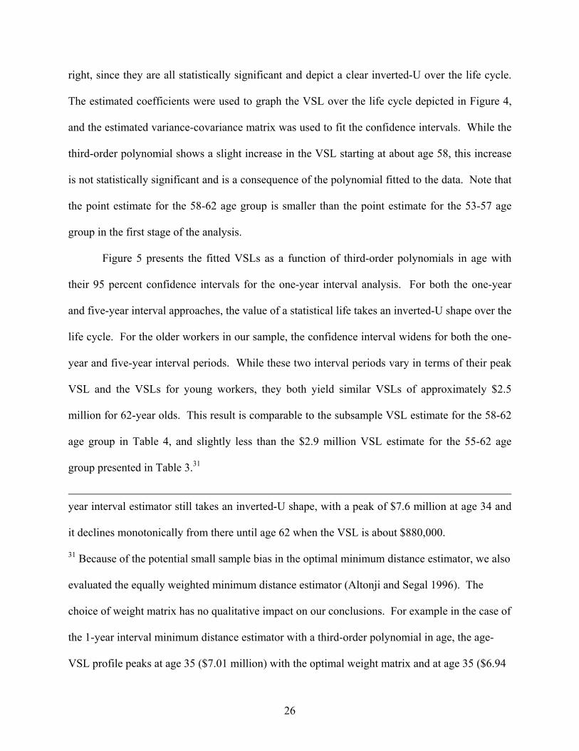
right, since they are all statistically significant and depict a clear inverted-U over the life cycle.

The estimated coefficients were used to graph the VSL over the life cycle depicted in Figure 4,

and the estimated variance-covariance matrix was used to fit the confidence intervals. While the

third-order polynomial shows a slight increase in the VSL starting at about age 58, this increase

is not statistically significant and is a consequence of the polynomial fitted to the data. Note that

the point estimate for the 58-62 age group is smaller than the point estimate for the 53-57 age

group in the first stage of the analysis.

Figure 5 presents the fitted VSLs as a function of third-order polynomials in age with

their 95 percent confidence intervals for the one-year interval analysis. For both the one-year

and five-year interval approaches, the value of a statistical life takes an inverted-U shape over the

life cycle. For the older workers in our sample, the confidence interval widens for both the one-

year and five-year interval periods. While these two interval periods vary in terms of their peak

VSL and the VSLs for young workers, they both yield similar VSLs of approximately $2.5

million for 62-year olds. This result is comparable to the subsample VSL estimate for the 58-62

age group in Table 4, and slightly less than the $2.9 million VSL estimate for the 55-62 age

group presented in Table 3.31

year interval estimator still takes an inverted-U shape, with a peak of $7.6 million at age 34 and

it declines monotonically from there until age 62 when the VSL is about $880,000.

31 Because of the potential small sample bias in the optimal minimum distance estimator, we also

evaluated the equally weighted minimum distance estimator (Altonji and Segal 1996). The

choice of weight matrix has no qualitative impact on our conclusions. For example in the case of

the 1-year interval minimum distance estimator with a third-order polynomial in age, the age-

VSL profile peaks at age 35 ($7.01 million) with the optimal weight matrix and at age 35 ($6.94

26

Finally, we tested the two propositions that characterize current policy applications of the

value of life: (1) the value of a statistical life is constant over the life cycle (as reflected in most

U.S. Environmental Protection Agency benefit-cost analyses, including September 2003

revisions to its assessment of the Clear Skies initiative), and (2) the value of a statistical life is

always decreasing with age (as reflected in the European Commission’s proposed position and

the life-year approach used by the U.S. Food and Drug Administration). To test the former

hypothesis, we specified the age polynomial function as a constant and employed the

overidentifying restrictions test presented in note 26. For both the one-year and five-year

interval periods, we reject the hypothesis that the value of life is constant over the workers’ life

cycle. In the case of the one-year interval estimator, the test statistic ranges from 443 to 540 for

comparisons of the constant function with polynomials of order two through six.32 In the case of

the five-year interval estimator, the test statistic ranges from 54.3 to 81.6 for the same

comparisons. For the latter hypothesis, we specified the age polynomial function as linear, but

such an approach yielded a negative coefficient estimate that clearly could not be distinguished

from zero. The test of overidentifying restrictions rejected the linear specification in comparison

to all higher order polynomials. It should also be noted that all order two through order six

million) with the equal weight matrix. Both decline monotonically from this peak to a VSL of

$2.35 million (optimal weight matrix) and $2.07 million (equally weighted matrix) at age 62.

For all specifications of the age polynomial, with both the one-year and five-year interval VSL

estimates, the age-VSL profiles take very similar shapes with comparable magnitudes for the two

approaches.

32 Note that ≤ 16.81 at the 1 percent level for the various tests comparing the constant

function with the higher order functions.

2χ

27

polynomials resulted in similar inverted U-shaped relationships between the value of a statistical

life and age.

D. Hedonic Wage Regressions with Age-Risk Interactions

We have also conducted hedonic wage regressions that include mortality risk and risk

interacted with age. This can serve as a comparison with the earlier hedonic wage literature

noted above and illustrate the potential pitfall of less flexible specifications of the data. Table 5

presents the age-risk interaction regression results and, as in the linear mortality risk regressions,

all regressors are statistically significant at the 1 percent level except for the Native American

indicator variable. The positive coefficient associated with the mortality risk variable and the

negative coefficient on the interaction of age and mortality risk imply that the compensating

differential for bearing mortality risk on the job should decrease with age, ceteris paribus. The

wage, however, is not constant over the worker’s life cycle, and the VSL derived from a semi-

log model is a linear function of the wage rate. The estimated VSL implied by these regressions

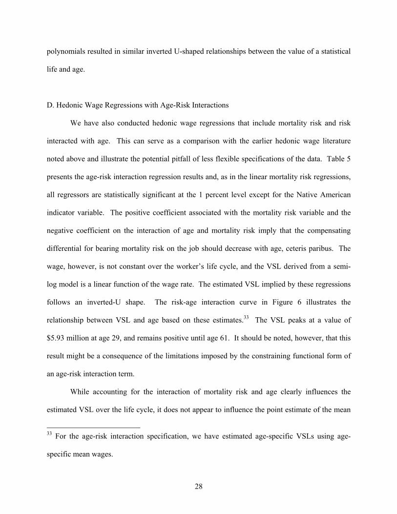
follows an inverted-U shape. The risk-age interaction curve in Figure 6 illustrates the

relationship between VSL and age based on these estimates.33 The VSL peaks at a value of

$5.93 million at age 29, and remains positive until age 61. It should be noted, however, that this

result might be a consequence of the limitations imposed by the constraining functional form of

an age-risk interaction term.

While accounting for the interaction of mortality risk and age clearly influences the

estimated VSL over the life cycle, it does not appear to influence the point estimate of the mean

33 For the age-risk interaction specification, we have estimated age-specific VSLs using age-

specific mean wages.

28

VSL for the sample. As a comparison of the last row in Tables 2 and 5 illustrates, estimates

using the linear mortality risk formulation and the mortality risk plus age-risk interaction yield

virtually identical VSL estimates when evaluated at sample means. A simple interaction of age

and risk may be too rigid a characterization of the age-specific income-risk tradeoff as evidenced

by the implausible negative VSLs for individuals aged 61 and 62 years in our analysis and for

earlier age groups in all previously published analyses. The coefficient estimates for mortality

risk and the interaction of risk and age are driven primarily by those aged 25-54, which comprise

more than 80 percent of our entire sample, and may produce a VSL function over age that may

fit the denser part of the data well but not the VSLs for those at the ends of the age distribution of

our sample.

E. The Effects of Life-Cycle Events on the Age-VSL Profile

We also evaluated whether the higher VSLs for individuals in the 25-44 age range reflect

major life-cycle events such as marriage or having children, and not variations in age. We

expanded the age-risk specifications to include a Mortality Risk*Married term in one regression

and a Mortality Risk*Children term in another (in which we also included Children, defined as

under 18 children residing with the worker, as an independent explanatory variable). If either of

these interactions are positive, and if it influences the magnitude and/or statistical significance of

the Mortality Risk*Age interaction, then the effects of age on the VSL revealed in the preceding

analyses may have actually reflected the effects of the family, and not one’s age, on the

estimated VSL.

In the case of marriage, the interaction of mortality risk and the married indicator variable

was not statistically significant, and the coefficient estimates on Mortality Risk and Mortality

29

Risk*Age were virtually unchanged from the specification reported in Table 5, Column 1. In the

case of children, we tested the effect of children by characterizing this variable as an indicator

variable for whether the worker has any children and as a discrete variable for the number of

children the worker has. In both cases, the interaction of Mortality Risk and Children was

statistically significant and negative, but it did not have a meaningful impact on the VSL, and the

coefficient estimates for the Mortality Risk and Mortality Risk*Age interaction variables were

still statistically significant at the one percent level and their magnitudes essentially unchanged.

We also included Mortality Risk*Married and Mortality Risk*Children interactions in the age

group regressions, but these were virtually all statistically insignificant. The variations in VSL

by age do not appear to be driven by changes in family status.

IV. Implications for the Value of a Statistical Life-Year

The preceding section illustrates the estimated age-VSL profile consistent with the theory

model presented in Section I and with previous simulations published in the literature. The

implicit assumptions underlying the value of a statistical life-year (VSLY) approach, which

require the value of life to be decreasing with age at all ages, are rejected by our data. In light of

the common application of VSLYs in evaluations of medical interventions, U.S. Food and Drug

Administration regulations, and in the sensitivity analyses of U.S. Environmental Protection

Agency regulations, we have estimated age-specific VSLYs based on our age-specific VSLs.

30

To construct values of statistical life-years, we have annuitized age-specific VSLs based

on age-specific years of life expectancy for 1996 (L) and an assumed discount rate of 3 percent

(r):34

(16) LrrVSLVSLY −+−

=)1(1

.

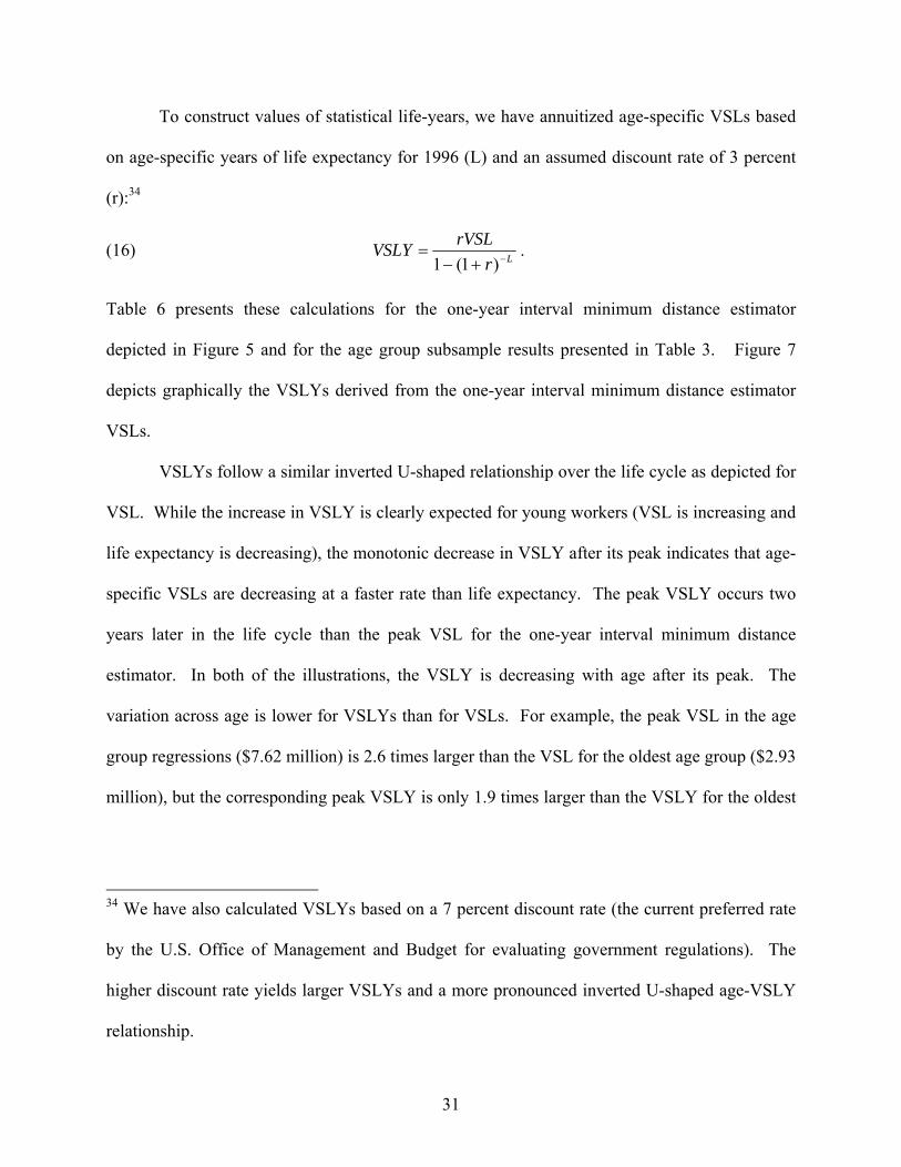
Table 6 presents these calculations for the one-year interval minimum distance estimator

depicted in Figure 5 and for the age group subsample results presented in Table 3. Figure 7

depicts graphically the VSLYs derived from the one-year interval minimum distance estimator

VSLs.

VSLYs follow a similar inverted U-shaped relationship over the life cycle as depicted for

VSL. While the increase in VSLY is clearly expected for young workers (VSL is increasing and

life expectancy is decreasing), the monotonic decrease in VSLY after its peak indicates that age-

specific VSLs are decreasing at a faster rate than life expectancy. The peak VSLY occurs two

years later in the life cycle than the peak VSL for the one-year interval minimum distance

estimator. In both of the illustrations, the VSLY is decreasing with age after its peak. The

variation across age is lower for VSLYs than for VSLs. For example, the peak VSL in the age

group regressions ($7.62 million) is 2.6 times larger than the VSL for the oldest age group ($2.93

million), but the corresponding peak VSLY is only 1.9 times larger than the VSLY for the oldest

34 We have also calculated VSLYs based on a 7 percent discount rate (the current preferred rate

by the U.S. Office of Management and Budget for evaluating government regulations). The

higher discount rate yields larger VSLYs and a more pronounced inverted U-shaped age-VSLY

relationship.

31

age group. While VSLY decreases with age after its peak based on our analyses, it does so at a

decreasing rate.

V. Conclusion

The implications of wage-risk tradeoffs for the dependency of VSL on age is consistent

based on all three sets of empirical estimates: separate age groups’ VSLs, a minimum distance

estimator derived from age-specific VSLs, and age-risk interaction estimates. For each case, the

VSL rises and then falls with age, displaying an inverted U-shaped relationship. The minimum

distance estimator results are perhaps most instructive, as they indicate a reasonably flat

inverted-U. In terms of the appropriate “senior discount,” workers in our sample in their early

60s have a VSL of $2.5-$3.0 million, which is about 30-40 percent lower than the market

average and between one-third and one-half the size of the VSLs for prime-aged workers.

The result that the VSL rises and falls with age is of both theoretical and policy interest.

Theoretical analysis of VSL over the life cycle suggests such a relationship may exist,

particularly in situations in which there are insurance and capital market imperfections. The

results are supportive of these models rather than those that generate steadily declining VSL with

age, such as some models with perfect annuity and insurance markets. VSL is not steadily

declining with age even though the amount of expected lifetime at stake, which is the good being

traded, steadily declines with age. As the life-cycle models indicate, this result is not surprising

since the age-VSL linkage depends on factors such as the life-cycle consumption pattern, which

also displays a similar temporal structure.

In terms of policy implications, this analysis does not provide support for approaches that

focus only on the remaining quantity of life as the valued attribute. Both the value per life-year

32

approach and the quality-adjusted life year methodology yield a steadily decreasing VSL with

age, whereas the revealed preferences of workers’ risk decisions indicate a quite different

relationship that rises and then declines with age. Explicit construction of age-specific values of

statistical life-years from our age-VSL profiles show that the value of a statistical life-year varies

with age. Likewise, there is no support for the standard practice of transferring VSLs from

studies based on the average of the labor market to risk contexts specific to the elderly

population. There is an inverted U-shaped relationship with a fairly flat upper tail in our sample.

Individuals make decisions over risk and income that clearly indicates that the value of their life

varies with age, but the relationship is not a simple one.

33

References

Altonji, J.G. and L.M. Segal. (1996). “Small-Sample Bias in GMM Estimation of Covariance

Structures.” Journal of Business and Economic Statistics 14(3): 353-366.

Anderson, R.N. (1998). United States Abridged Life Tables, 1996. National Vital Statistics

Reports 47(13).

Arnould, R.J. and L.M. Nichols. (1983). “Wage-Risk Premiums and Workers’ Compensation: A

Refinement of Estimates of Compensating Wage Differential.” Journal of Political

Economy 91(2): 332-340.

Arthur, W.B. (1981). “The Economics of Risks to Life.” American Economic Review 71(1): 54-

64.

Baranzini, A. and G. Ferro Luzzi. (2001). “The Economic Value of Risks to Life: Evidence

from the Swiss Labour Market.” Swiss Journal of Economics and Statistics 137(2): 149-

170.

Chamberlain, G. (1984). “Panel Data.” In: Z. Griliches and M.D. Intriligator, (eds.), Handbook

of Econometrics, Volume II, pages 1247-1318.

34

Corso, P.S., J.K. Hammitt, and J.D. Graham. (2001). “Valuing Mortality-Risk Reduction: Using

Visual Aids to Improve the Validity of Contingent Valuation.” Journal of Risk and

Uncertainty 23(2): 165-184.

Cropper, M.L. and F.G. Sussman. (1988). “Families and the Economics of Risks to Life.”

American Economic Review 78(1): 255-260.

Dreyfus, M.K. and W.K. Viscusi. (1995). “Rates of Time Preference and Consumer Valuations

of Automobile Safety and Fuel Efficiency.” Journal of Law and Economics 38: 79-105.

European Commission. (2001). “Recommended Interim Values for the Value of Preventing a

Fatality in DG Environment Cost Benefit Analysis.” Internet:

http://europa.eu.int/comm/environment/enveco/others/recommended_interim_values.pdf

Hammitt, J.K. and J.-T. Liu. (2004). “Effects of Disease Type and Latency on the Value of

Mortality Risk.” Journal of Risk and Uncertainty 28(1): 73-95.

Hara Associates Inc. (2000). Benefit/Cost Analysis of Proposed Tobacco Products Information

Regulations. Prepared for Health Canada and Consulting and Audit Canada. Ottawa,

Ontario. June 5, 2000.

Hersch, J. (1998). “Compensating Differentials for Gender-Specific Job Injury Risks.”

American Economic Review 88(3): 598-627.

35

Johannesson, M., P.-O. Johansson, and K.-G. Lofgren. (1997). “On the Value of Changes in Life

Expectancy: Blips Versus Parametric Changes.” Journal of Risk and Uncertainty 15:

221-239.

Johansson, P.-O. (2002). “On the Definition and Age-Dependency of the Value of a Statistical

Life.” Journal of Risk and Uncertainty 25(3): 251-263.

——— (2001). “Is there a Meaningful Definition of the Value of a Statistical Life?” Journal of

Health Economics 20: 131-139.

——— (1996). “On the Value of Changes in Life Expectancy.” Journal of Health Economics

15: 105-113.

Jones-Lee, M.W. (1976). The Value of Life: An Economic Analysis. Chicago: University of

Chicago Press.

Jones-Lee, M.W. (1989). The Economics of Safety and Physical Risk. Oxford: Basil Blackwell.

Jones-Lee, M.W., W.M. Hammerton, and P.R. Philips. (1985). “The Value of Safety: Results of

a National Sample Survey.” Economic Journal 95: 49-72.

36

Krupnick, A., Alberini, A., Cropper, M., Simon, N., O’Brien, B., Goeree, R., and Heintzelman,

M. (2002). “Age, Health, and the Willingness to Pay for Mortality Risk Reductions: A

Contingent Valuation Survey of Ontario Residents.” Journal of Risk and Uncertainty

24(2): 161-186.

Leeth, J.D. and J. Ruser. (2003). “Compensating Wage Differentials for Fatal and Nonfatal

Injury Risk by Gender and Race.” Journal of Risk and Uncertainty 27(3): 257-277.

Meng, R. (1989). “Compensating Differences in the Canadian Labour Market.” Canadian

Journal of Economics 22(2): 413-424.

Meng, R.A. and D.A. Smith. (1990). “The Valuation of Risk of Death in Public Sector

Decision-Making.” Canadian Public Policy - Analyse de Politiques 16(2): 137-144.

Moore, M.J. and W.K. Viscusi. (1990). “Models for Estimating Discount Rates for Long-Term

Health Risks Using Labor Market Data.” Journal of Risk and Uncertainty 3: 381-401.

National Safety Council. (2002). Injury Facts, 2002 Edition. Itasca, IL: National Safety

Council.

Persson, U., A. Norinder, K. Hjalte, and K. Gralen. (2001). “The Value of a Statistical Life in

Transport: Findings from a New Contingent Valuation Study in Sweden.” Journal of Risk

and Uncertainty 23(2): 121-134.

37

Rosen, S. (1988). “The Value of Changes in Life Expectancy.” Journal of Risk and Uncertainty

1: 285-304.

Shanmugam, K.R. (1996/7). “The Value of Life: Estimates from Indian Labour Market.”

Indian Economic Journal 44(4): 105-114.

Shanmugam, K.R. (2001). “Self Selection Bias in the Estimates of Compensating Differentials

for Job Risks in India.” Journal of Risk and Uncertainty 22(3): 263-275.

Shepard, D.S. and R.J. Zeckhauser. (1984). “Survival Versus Consumption.” Management

Science 30(4): 423-439.

Smith, V.K. and W.H. Desvousges. (1987). “An Empirical Analysis of the Economic Value of

Risk Changes.” Journal of Political Economy 95(1): 89-114.

Smith, V.K., M.F. Evans, H. Kim, and D.H. Taylor. (2004). “Do the ‘Near’ Elderly Value

Mortality Risks Differently?” Review of Economics and Statistics, forthcoming.

Thaler, R. and S. Rosen. (1975). “The Value of Saving a life: Evidence from the Labor Market.”

In: N.E. Terleckyj, (ed.), Household Production and Consumption. New York: Columbia

University Press. Pp. 265-298.

38

Viscusi, W.K. (1979). Employment Hazards: An Investigation of Market Performance.

Cambridge, MA: Harvard University Press.

Viscusi, W.K. (2004). The Value of Life: Estimates with Risks by Occupation and Industry.

Economic Inquiry 42(1): 29-48.

Viscusi, W.K. and J.E. Aldy. (2003). “The Value of a Statistical Life: A Critical Review of

Market Estimates Throughout the World.” Journal of Risk and Uncertainty 27(1): 5-76.

Viscusi, W.K. and J. Hersch. (2001). “Cigarette Smokers as Job Risk Takers.” Review of

Economics and Statistics 83 (2): 269-280.

39

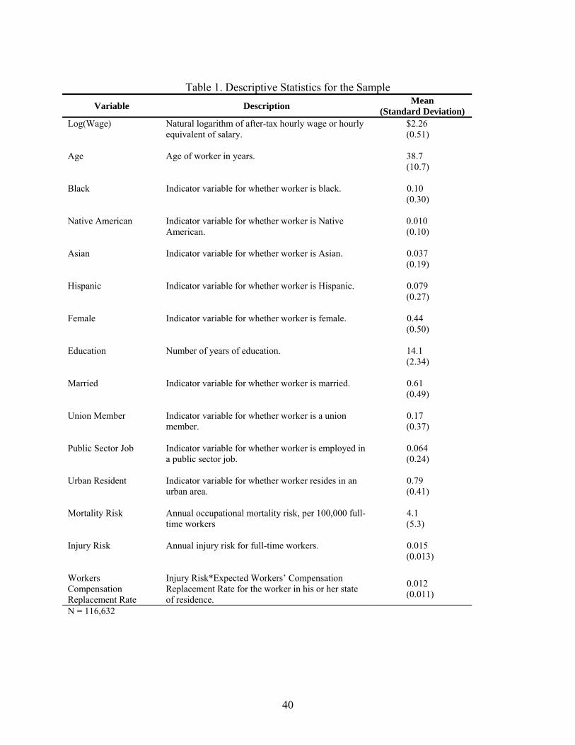
Table 1. Descriptive Statistics for the Sample

Variable Description Mean (Standard Deviation)

Log(Wage) Natural logarithm of after-tax hourly wage or hourly equivalent of salary.

$2.26 (0.51)

Age Age of worker in years. 38.7

(10.7) Black Indicator variable for whether worker is black. 0.10

(0.30) Native American Indicator variable for whether worker is Native

American. 0.010 (0.10)

Asian Indicator variable for whether worker is Asian. 0.037

(0.19) Hispanic Indicator variable for whether worker is Hispanic. 0.079

(0.27) Female Indicator variable for whether worker is female. 0.44

(0.50) Education Number of years of education. 14.1

(2.34) Married Indicator variable for whether worker is married. 0.61

(0.49) Union Member Indicator variable for whether worker is a union

member. 0.17 (0.37)

Public Sector Job Indicator variable for whether worker is employed in

a public sector job. 0.064 (0.24)

Urban Resident Indicator variable for whether worker resides in an

urban area. 0.79 (0.41)

Mortality Risk Annual occupational mortality risk, per 100,000 full-

time workers 4.1(5.3)

Injury Risk Annual injury risk for full-time workers. 0.015

(0.013) Workers Compensation Replacement Rate

Injury Risk*Expected Workers’ Compensation Replacement Rate for the worker in his or her state of residence.

0.012 (0.011)

N = 116,632

40

Table 2. Standard Hedonic Wage Regression Results Variable OLS

(1) 2SLS

(2) Age 0.0435

(0.00070)* [0.00085]*

0.0425 (0.0011)* [0.0024]*

Age2 -0.000454

(8.7x10-6)* [1.1x10-5]*

-0.000443 (1.2x10-5)* [2.4x10-5]*

Black -0.112

(0.0036)* [0.0041]*

-0.111 (0.0037)* [0.0044]*

Native American -0.0199

(0.011) [0.016]

-0.0206 (0.011)***

[0.016] Asian -0.0733

(0.0058)* [0.0079]*

-0.0711 (0.0060)* [0.0093]*

Hispanic -0.0830

(0.0042)* [0.0065]*

-0.0826 (0.0042)* [0.0066]*

Female -0.186

(0.0024)* [0.0040]*

-0.180 (0.0057)* [0.014]*

Education 0.0502

(0.00060)* [0.00091]*

0.0488 (0.0013)* [0.0031]*

Married 0.0694

(0.0023)* [0.0026]*

0.0617 (0.0069)* [0.017]*

Union Member 0.126

(0.0028)* [0.0057]*

0.125 (0.0030)* [0.0062]*

Public Sector Job 0.106

(0.0048)* [0.011]*

0.110 (0.0058)* [0.015]*

Urban Resident 0.0965

(0.0026)* [0.0043]*

0.0928 (0.0041)* [0.0092]*

Mortality Risk 0.00189

(0.00024)* [0.00052]*

0.00178 (0.00026)* [0.00058]*

41

Variable OLS (1)

2SLS (2)

Injury Risk 44.073

(0.37)* [1.04]*

52.297 (6.92)* [18.20]*

Workers Compensation Replacement Rate

-53.826 (0.46)* [1.27]*

-63.997 (8.55)* [22.52]*

Constant 0.446

(0.016)* [0.024]*

0.500 (0.048)* [0.12]*

R2 0.532 - N 116,632 116,632 Mean In-Sample VSL (95 percent confidence interval) (millions 96$)

$4.23 ($3.20 - $5.27)

$3.99 ($2.85 - $5.13)

Dependent Variable: natural logarithm of hourly labor income.

All specifications include 9 1-digit occupation indicator variables and 8 regional indicator variables.

Robust (White) standard errors are presented in parentheses and standard errors accounting for within-group

correlation are presented in brackets. The 95 percent confidence intervals are based on the robust standard errors.

The two-stage least squares regression instruments the expected workers’ compensation replacement rate with an

indicator variable for whether the state has a Republican governor and the state’s average workers’ compensation

benefit.

* Indicates statistical significance at 1 percent level, two-tailed test.

** Indicates statistical significance at 5 percent level, two-tailed test.

*** Indicates statistical significance at 10 percent level, two-tailed test.

42

Table 3. Age Group Subsample Hedonic Wage Regressions 18-24

Age Group 25-34

Age Group 35-44

Age Group 45-54

Age Group 55-62

Age Group

Mortality Risk 0.00255 (0.00079)* [0.00090]*

0.00350 (0.00046)* [0.00068]*

0.00314 (0.00048)* [0.00088]*

0.00153 (0.00046)* [0.00072]**

0.00120 (0.00061)**

[0.00070]***

R2 0.286 0.448 0.515 0.534 0.550

N 11,641 32,774 35,611 26,731 9,875

Mean In-Sample VSL (95 percent confidence interval) (millions 96$)

$3.42 ($1.34 - $5.49)

$7.06 ($5.26 - $8.87)

$7.62 ($5.32 - $9.92)

$3.92 ($1.60 - $6.24)

$2.93 ($0.016 - $5.85)

Dependent Variable: natural logarithm of hourly labor income.

All specifications include the same set of control variables as those presented in columns (1) – (4) in Table 2.

Robust (White) standard errors are presented in parentheses and clustered standard errors are presented in brackets.

The 95 percent confidence intervals are based on the robust standard errors.

* Indicates statistical significance at 1 percent level, two-tailed test.

** Indicates statistical significance at 5 percent level, two-tailed test.

** Indicates statistical significance at 10 percent level, two-tailed test.

43

Table 4. Minimum Distance Estimator Based on 5-Year Interval VSLs 1st Stage

Age Group VSL (millions 1996$)

18-22 $3.13*

23-27 $4.14*

28-32 $5.76*

33-37 $5.68*

38-42 $4.83*

43-47 $3.63*

48-52 $3.12**

53-57 $2.85**

58-62 $2.51***

2nd Stage Variable Coefficient Estimate

age 1.88x106

(1.41x106) age2 -4.54x104

(3.59x104) age3 335.24

(293.26) constant -1.92x107

(1.76x107) N 9

Asymptotic standard errors are presented in parentheses.

* Indicates mortality risk variable coefficient used to construct VSL statistically significant at 1 percent level, two-

tailed test.

** Indicates mortality risk variable coefficient used to construct VSL statistically significant at 5 percent level, two-

tailed test.

*** Indicates mortality risk variable coefficient used to construct VSL statistically significant at 10 percent level,

two-tailed test.

44

Table 5. Hedonic Wage Regression Results with Age-Risk Interaction Specification Variable OLS

(1) 2SLS

(2) Age 0.0434

(0.00070)* [0.00085]*

0.0424 (0.0011)* [0.0024]*

Age2 -0.000448

(8.8x10-6)* [1.1x10-5]*

-0.000437 (0.000013)* [2.6x10-5]*

Black -0.112

(0.0036)* [0.0041]*

-0.111 (0.0037)* [0.0044]*

Native American -0.0198

(0.011) [0.016]

-0.0205 (0.011)***

[0.016] Asian -0.0732

(0.0058)* [0.0079]*

-0.0709 (0.0061)* [0.0094]*

Hispanic -0.0832

(0.0042)* [0.0065]*

-0.0828 (0.0042)* [0.0066]*

Female -0.186

(0.0024)* [0.0040]*

-0.180 (0.0057)* [0.0014]*

Education 0.0501

(0.00060)* [0.00091]*

0.0487 (0.0013)* [0.0032]*

Married 0.0695

(0.0023)* [0.0026]*

0.0618 (0.0069)* [0.017]*

Union Member 0.126

(0.0028)* [0.0057]*

0.125 (0.0030)* [0.0062]*

Public Sector Job 0.104

(0.0048)* [0.011]*

0.108 (0.0057)* [0.014]*

Urban Resident 0.0965

(0.0026)* [0.0043]*

0.0927 (0.0041)* [0.0092]*

Mortality Risk 0.00563

(0.00091)* [0.0012]*

0.00618 (0.0011)* [0.0018]*

45

Variable OLS (1)

2SLS (2)

Mortality Risk*Age -9.23x10-5

(2.0x10-5)* [2.4x10-5]*

-0.000109 (2.5x10-5)*

[4.5x10-5]** Injury Risk 44.106

(0.37) * [1.03] *

52.317 (6.92)* [18.23]*

Workers Compensation Replacement Rate

-53.889 (0.46)* [1.27]*

-64.049 (8.56)* [22.57]*

Constant 0.440

(0.016)* [0.024]*

0.493 (0.047)* [0.12]*

R2 0.532 - N 116,632 116,632 Mean In-Sample VSL (millions 96$)

$4.28

$4.05

Dependent Variable: natural logarithm of hourly labor income.

All specifications include 9 1-digit occupation indicator variables and 8 regional indicator variables.

Robust (White) standard errors are presented in parentheses and standard errors accounting for within-group

correlation are presented in brackets. The two-stage least squares regression instruments the expected workers’

compensation replacement rate with an indicator variable for whether the state has a Republican governor and the

state’s average workers’ compensation benefit.

* Indicates statistical significance at 1 percent level, two-tailed test.

** Indicates statistical significance at 5 percent level, two-tailed test.

*** Indicates statistical significance at 10 percent level, two-tailed test.

46

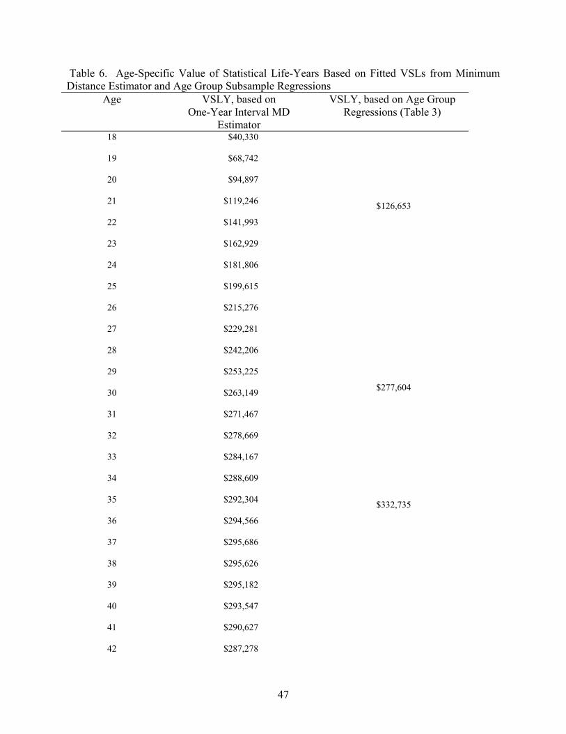
Table 6. Age-Specific Value of Statistical Life-Years Based on Fitted VSLs from Minimum Distance Estimator and Age Group Subsample Regressions

Age VSLY, based on One-Year Interval MD

Estimator

VSLY, based on Age Group Regressions (Table 3)

18 $40,330

19 $68,742

20 $94,897

21 $119,246

22 $141,993

23 $162,929

24 $181,806

$126,653

25 $199,615

26 $215,276

27 $229,281

28 $242,206

29 $253,225

30 $263,149

31 $271,467

32 $278,669

33 $284,167

34 $288,609

$277,604

35 $292,304

36 $294,566

37 $295,686

38 $295,626

39 $295,182

40 $293,547

41 $290,627

42 $287,278

$332,735

47

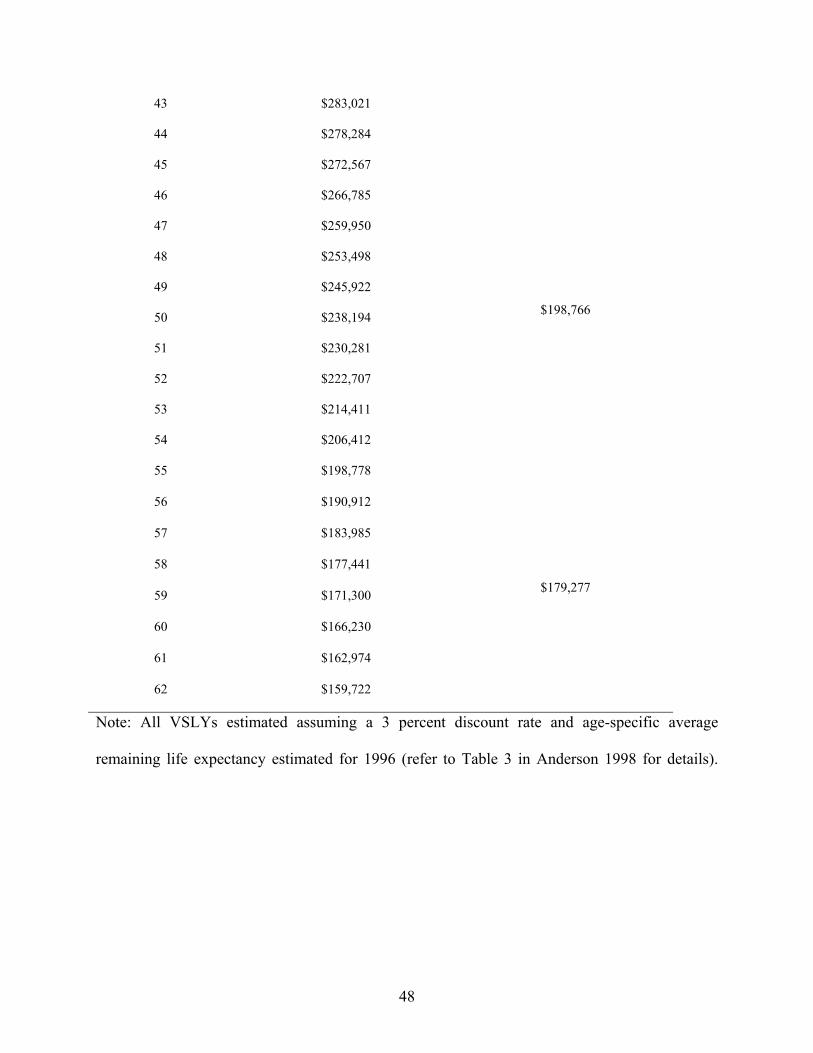
43 $283,021

44 $278,284

45 $272,567

46 $266,785

47 $259,950

48 $253,498

49 $245,922

50 $238,194

51 $230,281

52 $222,707

53 $214,411

54 $206,412

$198,766

55 $198,778

56 $190,912

57 $183,985

58 $177,441

59 $171,300

60 $166,230

61 $162,974

62 $159,722

$179,277

Note: All VSLYs estimated assuming a 3 percent discount rate and age-specific average

remaining life expectancy estimated for 1996 (refer to Table 3 in Anderson 1998 for details).

48

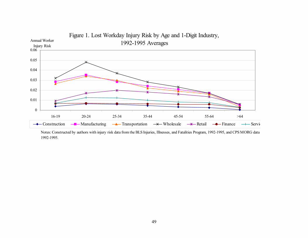
Figure 1. Lost Workday Injury Risk by Age and 1-Digit Industry, 1992-1995 Averages

0

0.01

0.02

0.03

0.04

0.05

0.06

16-19 20-24 25-34 35-44 45-54 55-64 >64

Annual Worker Injury Risk

Construction Manufacturing Transportation Wholesale Retail Finance Servic

Notes: Constructed by authors with injury risk data from the BLS Injuries, Illnesses, and Fatalities Program, 1992-1995, and CPS MORG data 1992-1995.

49

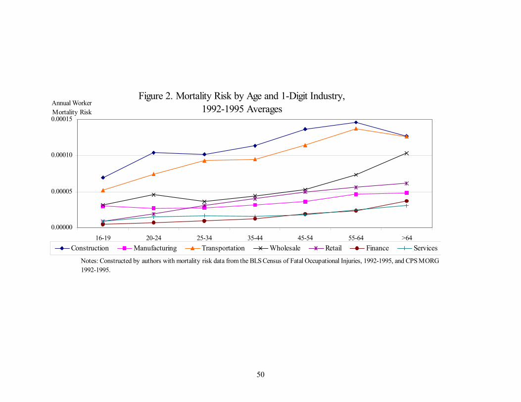
Figure 2. Mortality Risk by Age and 1-Digit Industry, 1992-1995 Averages

0.00000

0.00005

0.00010

0.00015

16-19 20-24 25-34 35-44 45-54 55-64 >64

Annual Worker Mortality Risk

Construction Manufacturing Transportation Wholesale Retail Finance Services

Notes: Constructed by authors with mortality risk data from the BLS Census of Fatal Occupational Injuries, 1992-1995, and CPS MORG 1992-1995.

50

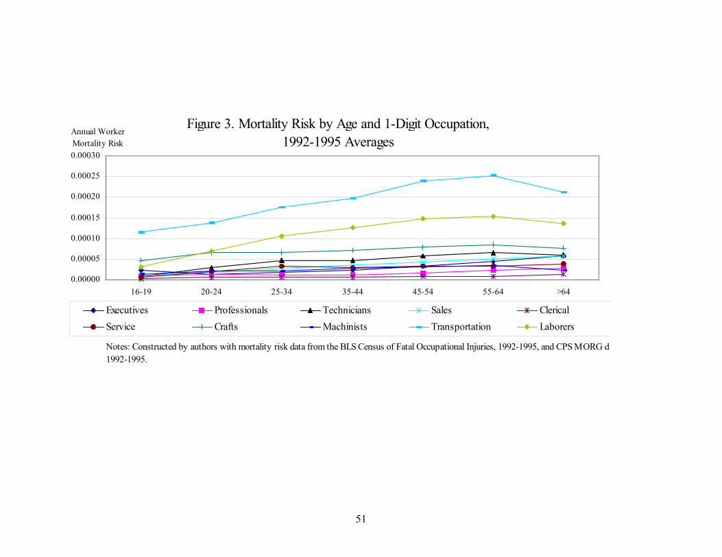
Figure 3. Mortality Risk by Age and 1-Digit Occupation, 1992-1995 Averages

0.00000

0.00005

0.00010

0.00015

0.00020

0.00025

0.00030

16-19 20-24 25-34 35-44 45-54 55-64 >64

Annual Worker Mortality Risk

Executives Professionals Technicians Sales ClericalService Crafts Machinists Transportation Laborers

Notes: Constructed by authors with mortality risk data from the BLS Census of Fatal Occupational Injuries, 1992-1995, and CPS MORG da1992-1995.

51

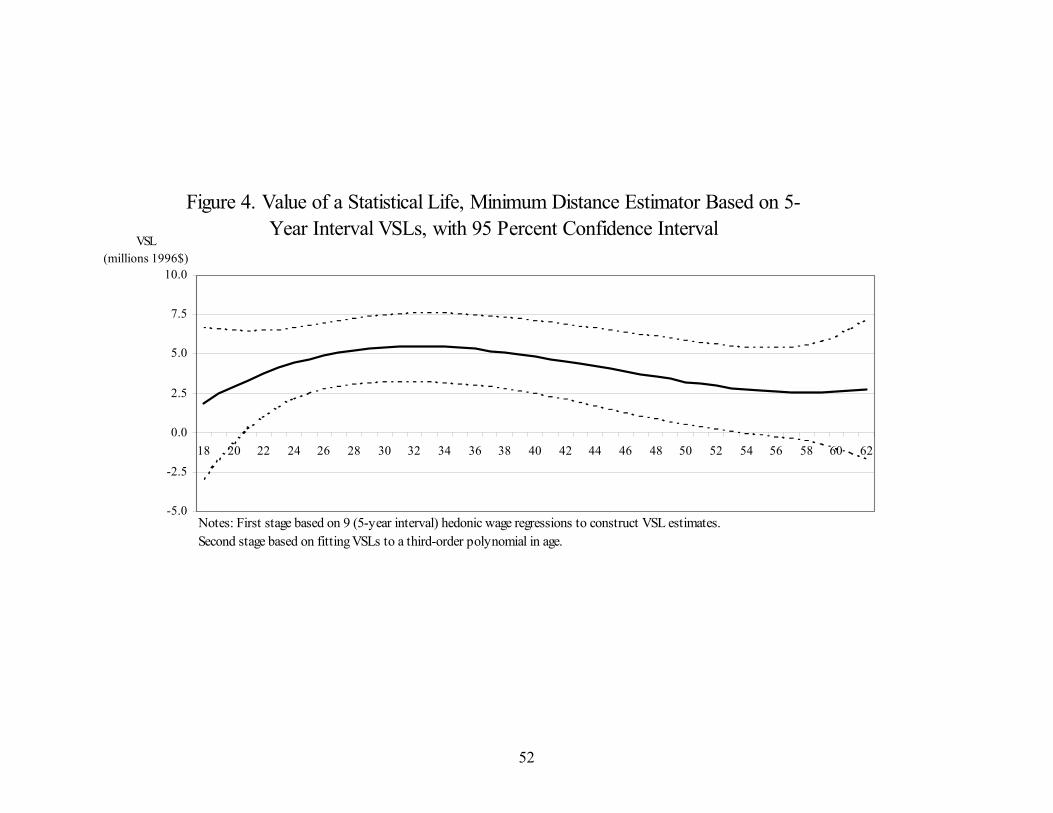
Figure 4. Value of a Statistical Life, Minimum Distance Estimator Based on 5-Year Interval VSLs, with 95 Percent Confidence Interval

-5.0

-2.5

0.0

2.5

5.0

7.5

10.0

18 20 22 24 26 28 30 32 34 36 38 40 42 44 46 48 50 52 54 56 58 60 62

VSL (millions 1996$)

Notes: First stage based on 9 (5-year interval) hedonic wage regressions to construct VSL estimates. Second stage based on fitting VSLs to a third-order polynomial in age.

52

Figure 5. Value of a Statistical Life, Minimum Distance Estimator Based on 1-Year Interval VSLs, with 95 Percent Confidence Interval

-5.0

-2.5

0.0

2.5

5.0

7.5

10.0

18 20 22 24 26 28 30 32 34 36 38 40 42 44 46 48 50 52 54 56 58 60 62

VSL (millions 1996$)

Notes: First stage based on 45 year-specific hedonic wage regressions to construct age-specific VSLs. Second stage based on fitting VSLs to a third-order polynomial in age.

53

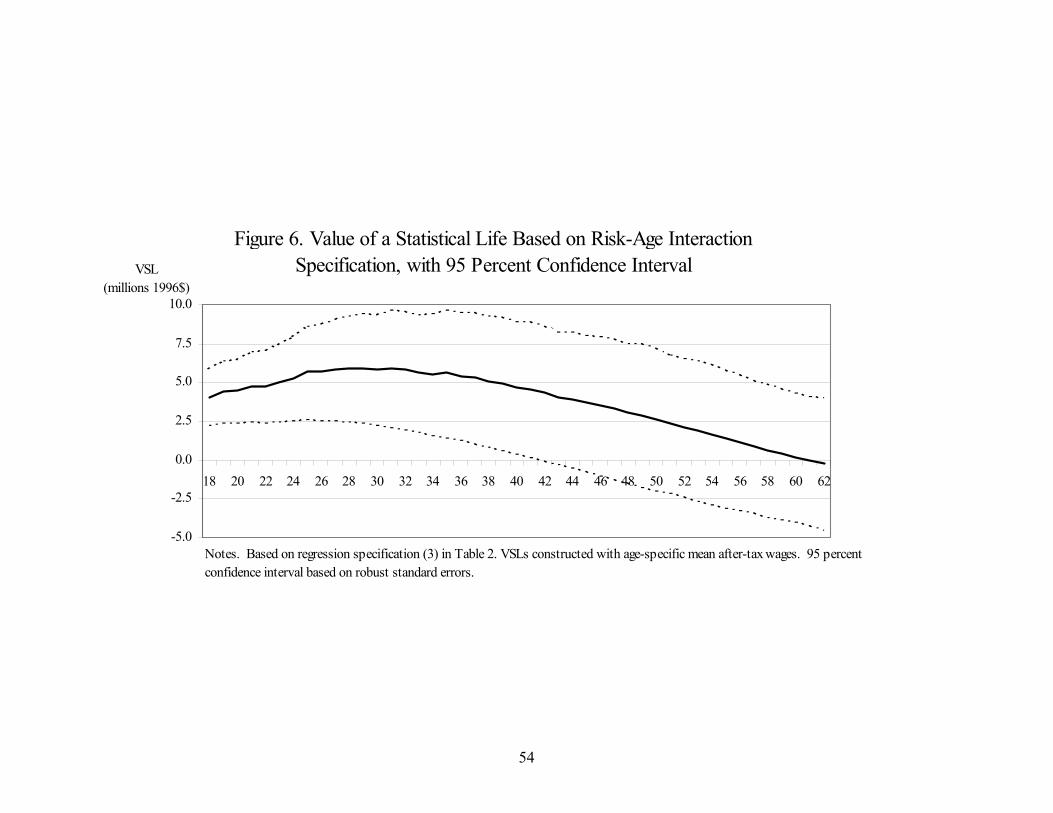
Figure 6. Value of a Statistical Life Based on Risk-Age Interaction Specification, with 95 Percent Confidence Interval

-5.0

-2.5

0.0

2.5

5.0

7.5

10.0

18 20 22 24 26 28 30 32 34 36 38 40 42 44 46 48 50 52 54 56 58 60 62

VSL (millions 1996$)

Notes. Based on regression specification (3) in Table 2. VSLs constructed with age-specific mean after-tax wages. 95 percent confidence interval based on robust standard errors.

54

Figure 7. Age-Specific Value of Statistical Life Years Based on One-Year Minimum Distance Estimator Fitted VSLs

$0

$50,000

$100,000

$150,000

$200,000

$250,000

$300,000

$350,000

18 20 22 24 26 28 30 32 34 36 38 40 42 44 46 48 50 52 54 56 58 60 62

VSLY (1996$)

Note: All VSLYs constructed from Figure 5 VSLs assuming a 3 percent discount rate and age-specific remaining life expectancy for 1996.

55