IS THE CARIBBEAN COMMUNITY AN OPTIMUM … Studies of International Development Vol. 8-1 (2008) IS THE CARIBBEAN COMMUNITY AN OPTIMUM CURRENCY AREA? GHARTEY, Edward E.* Abstract This

Economic Studies of International Development Vol. 8-1 (2008)

IS THE CARIBBEAN COMMUNITY AN OPTIMUM CURRENCY AREA?

GHARTEY, Edward E.* Abstract This study analyzes the viability of the Caribbean Market Economies (CME) as an optimum currency area. A vector error correction model is used with cointegration as an identifying restriction to decompose real output, prices and exchange rate into supply, demand and monetary shocks. Respective shocks are then tested for symmetry between countries to assess their suitability in meeting the optimum currency area (OCA) criteria. The US is used to capture global effects in assessing the convergence of the optimum OCA criteria. It is then used as a yardstick to compare size of shocks and speed of adjustment to those shocks to determine the viability of the CME as an optimum currency area. Shocking results from impulse response functions show that the Eastern Caribbean Currency Area (ECCA) members meet the OCA convergence criteria better than the non-ECCA members. However, the overall results depict that the Caribbean Community are not a suitable OCA as some of their correlation results are asymmetrical, and have large size of shocks and slow speed of adjustment relative to the US. JEL: C22, E42, F15 and F33 Keywords: Vector error correction model, shocks, symmetry, optimum currency area, Caribbean Market Economy 1. Introduction

Developments leading to the formation of the European Union

in the 1990s have also prompted countries which share similar aspirations in the past to re-consider their commitment to succeed in developing into an economic union. Members of the Caribbean Community (CARICOM) have now decided to strengthen their commitment to form a viable CARICOM Single Market and Economy

* Edward E. Ghartey, Ph.D.Department of Economics, The University of the West Indies, Kingston 7, Jamaica, Email: [email protected]


6

(CSME)1. Their intended goals are to: (a) present a common international voice in their negotiations as a response to the World Trade Organization’s removal of preferential treatments extended to Africa, Caribbean and Pacific Countries (APC) in 2007, (b) enter the Free Trade Area of Americas (FTAA), (c) effectively deal with the North American Free Trade Area (NAFTA) and other emerging single market economies, and meet the European Union’s threat of not dealing with individual countries by January 2008, (d) hasten their effort to become a viable trade bloc by deepening economic and trade integration among members within the CARICOM Market Economy (CME), and (e) assist the region to decide on the adoption of a single currency and exchange rate system

A single market certainly requires a single currency such as the

Eastern Caribbean Currency Area (ECCA), but in the absence of a single currency, the states within the single market can adopt ‘irrevocable’ fixed exchange rates to become a common currency area. A precedent for the CARICOM is the exchange rate mechanism the European Communities adopted following the Maastricht Treaty in 1991. However, since not all CARICOM economies have a common currency, an exchange rate band could be set up for members to allow their national currencies to be adjusted within. It should be noted though that unlike a single market with a common currency, countries that adopt an ‘irrevocable’ fixed exchange rate within an accepted exchange rate band cannot experience full benefits members of a single currency enjoy, such as: a medium of exchange, a store of value, a unit of account and a standard of deferred payment. Additionally, members of ‘irrevocable’ fixed exchange rates systems can still exit to print their national monies without incurring any penalty (see Bean, 1992; Mundell, 1961; McKinnon, 1963; Kenen, 1969; Grubel, 1970).

The CARICOM members who oppose a single currency cite

macroeconomic costs such as loss of part of their seigniorage, and the fact that the stable prices a single currency carries in its trail may retard 1CARICOM was inaugurated on July 4, 1973 when the Treaty of Chaguaramus was signed. Heads of Government used the 1989 Grand Anse Declaration to change CARICOM to CSME in 1992.

Ghartey, E.E. Is The Caribbean Community An Optimum Currency Area?

7

economic growth. They also note that the road to convergence will be difficult because of the huge debt burden of Jamaica and Guyana with both countries debt to gross domestic product (GDP) ratios consistently exceeding 100 percent over the past five years. Notwithstanding these objections, adopting a single currency will reduce transaction costs, uncertainty and currency risk, stabilize prices and exchange rates, ensure low interest rates by imposing fiscal discipline, and promote economies of scale and efficiency. These benefits will be spurred from their combined population of more than 14.35 million over a total land area of 462,252 sq. km. 2. In fact by adopting a single currency, members of a regional bloc like the CME could improve their chances of meeting the optimum currency area (OCA) criteria ex-ante (Frankel and Rose, 1998, 2000); increase trade within the CARICOM, and ensure free mobility of capital, labor, goods and services among members in the region.

In view of the above, the paper tests the OCA criteria such as

symmetry of shocks across regional economies to be met by members of the CARICOM (Mundell, 1961). A shock is symmetric if it is positively correlated, and it is asymmetric if it is either negatively or insignificantly correlated. If shocks are distributed symmetrically across members of the CARICOM, then they can adopt a common fiscal or monetary policy in response to negative aggregate demand and supply shocks. Variability in output measured by the GDP, prices measured by the consumer price index (CPI), and exchange rate are used to determine the extent of asymmetric shocks. We have also measured relative sizes of underlying shocks and speed of adjustment to disturbances experienced by the CME members. Note, however, that even in a situation where members exhibit asymmetric shocks, if those shocks are small in size and members can respond faster to them, then by the OCA criteria, members of such an economic community can still benefit fully from adopting a common currency (see Bayoumi and Eichengreen, 1992).

2 These figures are 2006 estimates from the CIA Fact Book and they exclude the population and total area of Montserrat.


8

The study is outlined along the following format: Section 2 discusses the case for common currency for the CARICOM members. Data and sources are discussed, and the vector error correction model (VECM) is developed in section 3. Section 4 discusses the empirical results, and the paper is concluded in section 5 with some policy recommendations. 2: The CARICOM Market Economy and Common Currency

The literature on OCA presents a list of criteria for the use of a

single currency. These are (1) openness to mutual trade, (2) diversification of economies within the union, (3) mobility of factors of production across the union, (4) correlation of underlying shocks or convergence of business cycles among members, (5) similarities in characteristics, (6) flexibility in setting wages and prices to allow members to respond effectively to external shocks without depending on changes in interest rates and exchange rates, and (7) finally, versatile fiscal institutions to allow net transfers to replace immobile factors of production by ensuring a system of risk-sharing among members3 (see Mundell, 1961; McKinnon, 1963; Kenen, 1969; Grubel, 1970).

The CME members include The Bahamas, Barbados, Belize,

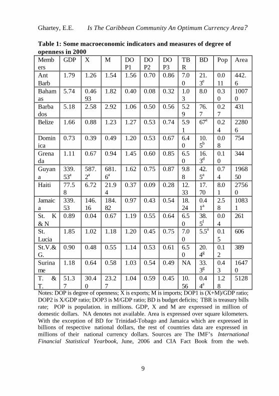
Guyana, Haiti, Jamaica, Suriname, Trinidad-Tobago, and the ECCA members comprise of Antigua and Barbuda, Dominica, Grenada, St. Kitts and Nevis, St. Lucia, and St. Vincent and The Grenadines. They share common characteristics which are different from the European Union (EU) members. They are all small economies in terms of their population size, and are highly open as measured by their degree of openness (DOP) (import/GDP) ratios which are more than 50 percent in 2000 with the exception of The Bahamas, Grenada, Haiti, Suriname and Trinidad-Tobago. In 2000 the DOP measured by total trade which is the sum of exports and imports as a ratio of the GDP is more than unity for all the members except The Bahamas, Haiti and Jamaica. See Table 1.

3 For a discussion on ‘New’ Theory of Optimum Currency Area (see Tavlas, 1993).


9

Table 1: Some macroeconomic indicators and measures of degree of openness in 2000 Members

GDP X M DOP1

DOP2

DOP3

TBR

BD Pop Area

Ant Barb

1.79 1.26 1.54 1.56 0.70 0.86 7.00

21.3e

0.011

442.6

Bahamas

5.74 0.4693

1.82 0.40 0.08 0.32 1.03

8.0 0.30

10070

Barbados

5.18 2.58 2.92 1.06 0.50 0.56 5.29

76.7

0.27

431

Belize 1.66 0.88 1.23 1.27 0.53 0.74 5.91

67a 0.24

22806

Dominica

0.73 0.39 0.49 1.20 0.53 0.67 6.40

10.5b

0.08

754

Grenada

1.11 0.67 0.94 1.45 0.60 0.85 6.50

16.3d

0.10

344

Guyana

339.53a

587.2a

681.6a

1.62 0.75 0.87 9.88

42.5a

0.74

196850

Haiti 77.58

6.72 21.94

0.37 0.09 0.28 12.33

17.70

8.01

27560

Jamaica

339.53

146.16

184.82

0.97 0.43 0.54 18.24

0.41a

2.58

10831

St. K & N

0.89 0.04 0.67 1.19 0.55 0.64 6.50

38.5f

0.04

261

St. Lucia

1.85 1.02 1.18 1.20 0.45 0.75 7.00

5.5a 0.15

606

St.V.&G.

0.90 0.48 0.55 1.14 0.53 0.61 6.50

20.4g

0.12

389

Suriname

1.18 0.64 0.58 1.03 0.54 0.49 NA 33.3g

0.43

16470

T. & T.

51.37

30.40

23.27

1.04 0.59 0.45 10.56

0.44a

1.28

5128

Notes: DOP is degree of openness; X is exports; M is imports; DOP1 is (X+M)/GDP ratio; DOP2 is X/GDP ratio; DOP3 is M/GDP ratio; BD is budget deficits; TBR is treasury bills rate; POP is population. in millions. GDP, X and M are expressed in million of domestic dollars. NA denotes not available. Area is expressed over square kilometers. With the exception of BD for Trinidad-Tobago and Jamaica which are expressed in billions of respective national dollars, the rest of countries data are expressed in millions of their national currency dollars. Sources are The IMF’s International Financial Statistical Yearbook, June, 2006 and CIA Fact Book from the web.


10

Superscripts:a denotes 2005 estimates, b denotes 2001 actual data, d denotes 1997 actual data, e denotes 2000 estimates, f denotes 2003 estimates, and g denotes 2004 actual data.

Herfindhal (H) indices4 defined as the sum of squares of shares of specific export products of each member measure degrees of trade specialization. They are relatively larger than 0.22 for the CME members except Barbados. Belize has the highest level of specialization among them with an H index of 0.64. The Bahamas, Trinidad-Tobago, Jamaica and Guyana are relatively less specialized with H indices ranging from 0.25 to 0.39. Thus by international standards, majority of members of the CME are specialized and have a much lower level of product diversification (Cf. Table 2a of Rose and Engel, 2000).

Furthermore, leading non-service exports among members with

the exception of Trinidad-Tobago and Antigua-Barbuda are food and living animals which make them suitable for the OCA under flexible exchange rates as their products are less diversified (see Kenen, 1969). Their degrees of specialization in international trade expose them to asymmetric shocks which make them vulnerable to meet Mundell’s OCA criteria.

The gravity model which is used to explain trade flows from country j to k shows that in international trade theory normally distance and GDP which are ‘pure’ economic determinants of bilateral trade between countries are expected to be significant with the coefficient of distance being negative. Summary (1989) found distance to be -0.59 for bilateral exports trade, and -0.62 for bilateral imports trade in 1978 between the US and sixty-six countries. His results are relatively smaller compared with (Manioc and Motauban’s, 2001) estimated coefficients of distance between members of the CARICOM which range from -1.39 to -1.27 in 1995. Note that the CARICOM results are larger than (Rose’s, 2000) estimated coefficients for the world which were -1.12 in 1990 and -

4 Hit = ∑=

=

Jj

j 1

(xijt/Xit)2 where xijt denotes export of SITC subgroup product j in

year t for country i, Xit denotes total export products of country i at year t, and it is summed over the entire SITC subgroups. H ranges from zero to unity. A high value of H implies that the country is specialized in few goods, whereas a low value of H implies that the country is well diversified.


11

1.03 in 1980, and were corrected to -1.09 in 1990 and -1.00 in 1980 by (Nitsch, 2002). Thus, distance between any two capitals of the CME members adversely affects their international trade within the CARICOM significantly than the world’s average. This means that the labor mobility criterion of the OCA is not easily met by the CME members because of lack of contiguity as most members are separated by the sea. Nevertheless, the fact that most members speak English and have a similar history reduces some of their barriers to labor mobility drastically. Note that among the members only Suriname and Haiti are non Anglophone.

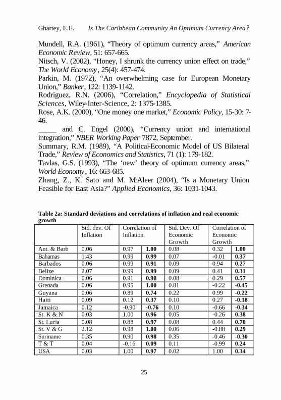
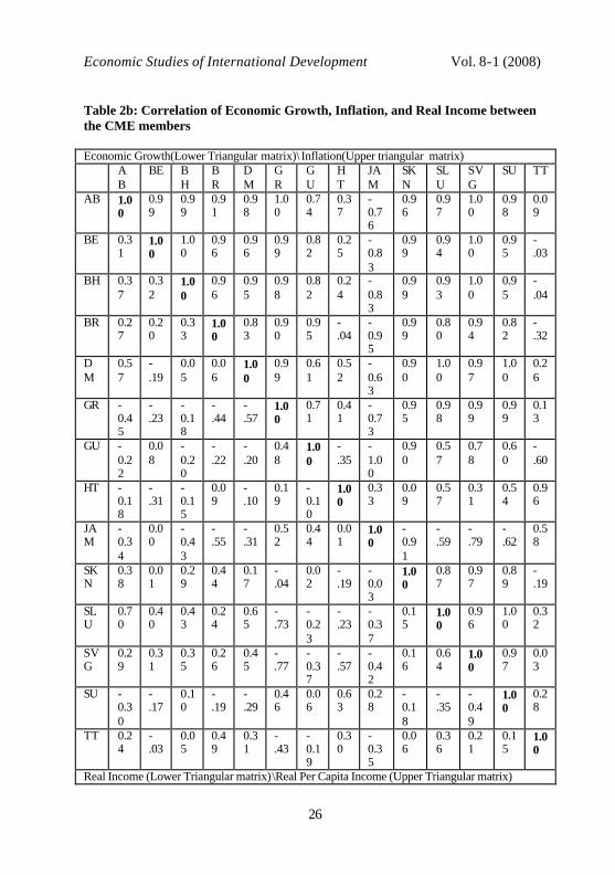
Correlation of inflation rates over the sample period between

members except Guyana, Haiti, Jamaica and Trinidad-Tobago are more than 90 percent using the US as a bench mark to capture global effects. Similar results are obtained when smaller islands such as Antigua-Barbuda or Grenada or St. Vincent and the Grenadines are used as a benchmark. See the boldfaced figures in Table 2a. Additionally, standard deviations of inflation rates are very low. Only The Bahamas, Belize, St. Vincent and the Grenadines, Jamaica and Suriname report inflation rates in excess of 12 percent. See Tables 2a and 2b. Note that the significance of inflation rate as an OCA criterion is contentious. For instance, (Fleming, 1971) considers it to be a very useful criterion because of policy implications of Phillips curve, although (Parkin, 1972) does not find it to be a useful criterion. Additionally, (Kenen, 1997) argues that the stability and growth pact to limit budget deficits, which is one of the convergence criteria for admission into the EMU, ensures price stability.

Countries with highly synchronized business cycles as measured

by correlation of economic growth and real GDP between them are more likely to succeed at adopting a common currency (Mundell, 1961). This criterion is met by some members of the CME because the real GDP between them are highly and systematically correlated, although some members experience negative correlation or acute asymmetric disturbance. See Tables 2a and 2b. But as argued by (Frankel and Rose, 2000), the formation of an OCA tends to foster a closer economic integration among members. Rose’s (2000) study finds that international


12

business cycle correlations increase by 10 percent between members of an OCA, although the ECCA members do not experience such benefit.

We have estimated structural shocks correlation between

members with a VECM which has real GDP, prices and exchange rates to capture supply, demand and monetary shocks, respectively. The US is included as an ideal monetary union instead of the EU to serve as a benchmark to capture global influences, and to provide a yardstick for comparison because apart from its proximity to the region, ‘Shocks to the US core and periphery show considerably more coherence than shocks to the analogous European region’ (Bayoumi and Eichengreen, 1992). We have also employed impulse response functions to measure relative sizes of shocks and their respective speed of adjustments between members. 3: The Model 3.1: The Vector Error Correction Model Bayoumi and Eichengreen (1992) employed correlation of shocks to determine the feasibility of OCA criteria for the European Countries using a vector autoregressive (VAR) model (Blanchard and Quah, 1989). They identified the VAR model by imposing restrictions to identify the Choleski decomposition of real output and prices into supply and demand shocks, respectively, from the following economic theory: (a) demand shocks have (i) positive effect on prices only in the long run, (ii) positive effect on both prices and output in the short-term; and in both short-term and long-run (b) supply shocks have (iii) negative effect on prices and (iv) positive effect on output. Other studies followed their methodology with some modifications (see Demertzis, et al. 2000; Zhang, et al. (2004).

In this study, we have employed the VECM to decompose real output, prices and exchange rates into underlying supply, demand and monetary shocks, respectively. Note that (Zhang, et al. 2004) decompose output, effective exchange rate and prices into supply, monetary and demand shocks, respectively, whereas (Demertzis, et al. 2000) used a simple VAR to decompose real output, relative prices and inflation into supply, demand and monetary shocks, respectively. The economic theory justification of the identifying restrictions they employed to obtain a lower triangular matrix of their simple VAR


13

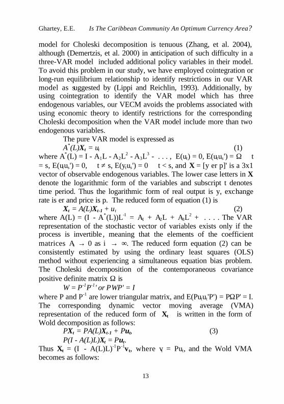
model for Choleski decomposition is tenuous (Zhang, et al. 2004), although (Demertzis, et al. 2000) in anticipation of such difficulty in a three-VAR model included additional policy variables in their model. To avoid this problem in our study, we have employed cointegration or long-run equilibrium relationship to identify restrictions in our VAR model as suggested by (Lippi and Reichlin, 1993). Additionally, by using cointegration to identify the VAR model which has three endogenous variables, our VECM avoids the problems associated with using economic theory to identify restrictions for the corresponding Choleski decomposition when the VAR model include more than two endogenous variables.

The pure VAR model is expressed as A*(L)Xt = ut (1)

where A*(L) = I - A1L - A2L2 - A3L3 - . . . , E(ut) = 0, E(utus') = Ω ∀ t = s, E(utus') = 0, ∀ t ≠ s, E(ytus') = 0 ∀ t < s, and X = [y er p]' is a 3x1 vector of observable endogenous variables. The lower case letters in X denote the logarithmic form of the variables and subscript t denotes time period. Thus the logarithmic form of real output is y, exchange rate is er and price is p. The reduced form of equation (1) is Xt = A(L)Xt-1 + ut (2) where A(L) = (I - A*(L))L-1 = A1 + A2L + A3L2 + . . . . The VAR representation of the stochastic vector of variables exists only if the process is invertible , meaning that the elements of the coefficient matrices Ai → 0 as i → ∞. The reduced form equation (2) can be consistently estimated by using the ordinary least squares (OLS) method without experiencing a simultaneous equation bias problem. The Choleski decomposition of the contemporaneous covariance positive definite matrix Ω is Ω = P-1P-1' or PΩP' = I where P and P-1 are lower triangular matrix, and E(Putut'P') = PΩP' = I. The corresponding dynamic vector moving average (VMA) representation of the reduced form of Xt is written in the form of Wold decomposition as follows: PXt = PA(L)Xt-1 + Put, (3) ⇒ P(I - A(L)L)Xt = Put. Thus Xt = (I - A(L)L)-1P-1vt, where vt = Put, and the Wold VMA becomes as follows:


14

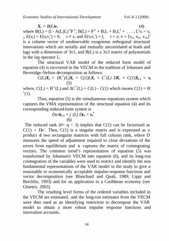
Xt = B(L)vt (4) where B(L) = (I - A(L)L)-1P-1; B(L) = P-1 + B1L + B2L2 + . . . ; Ljvt = vt-

j, E(vt) = E(vtvs') = 0, ∀ t ≠ s, and E(vtvs') = I, ∀ t = s; v = [vst, vdt, vmt]’ is a column vector of unobservable exogenous orthogonal structural innovations which are serially and mutually uncorrelated at leads and lags with a dimension of 3x1, and B(L) is a 3x3 matrix of polynomials in the lag operator L. The structural VAR model of the reduced form model of equation (4) is recovered in the VECM in the tradition of Johansen and Beveridge-Nelson decomposition as follows: C(L)Xt = ∆C*(L)Xt + C(1)LXt = C*(L) ∆Xt + C(1)Xt-1 = vt (5) where, C(L) = B-1(L) and ∆C*(L) = C(L) - C(1) which means C(1) = B-

1(1). Thus, equation (5) is the simultaneous-equations system which

captures the VMA representation of the structural equation (4) and its corresponding reduced-form system is

Dα′xt-1 + ϕ(L) ∆xt = vt*

(6) The reduced rank (0< q < 3) implies that C(1) can be factorized as C(1) = Dα′. Thus, C(1) is a singular matrix and is expressed as a product of two rectangular matrices with full column rank, where D measures the speed of adjustment required to close deviations of the errors from equilibrium and α captures the matrix of cointegrating vectors. The common trend’s representation of equation (5) was transformed by Johansen's VECM into equation (6), and its long-run cointegration of the variables were used to restrict and identify the non fundamental representations of the VAR model in the study to give a reasonable or economically acceptable impulse-response functions and vector decomposition (see Blanchard and Quah, 1989; Lippi and Reichlin, 1993) and for an application to a Caribbean economy (see Ghartey, 2003).

The resulting level forms of the ordered variables included in the VECM are estimated, and the long-run estimates from the VECM were then used as an identifying restriction to decompose the VAR model to obtain a more robust impulse response functions and innovation accounts.


15

The global effect of shocks on the CME members is estimated by including similar macroeconomic variables of the USA into the VECM to obtain correlation results to compare with our results. Our a priori expectation is that a positive and significant correlation in underlying shocks between countries implies that shocks are symmetric, so such economies will increase their trade by adopting a common currency. If the correlations are either negative or insignificant, then the shocks are asymmetric therefore adopting a common currency will not improve trade between them.

The impulse response functions are also used to measure the size of shocks and the speed of adjustment to disturbances. Note that asymmetric shocks are manageable if their sizes are small and members can adjust to them speedily. Again, we have included the US as a yardstick to assess the size of shocks and speed of adjustment to shocks by members. 3.2: Data Data on prices, output and exchange rates are sourced from various issues of the International Monetary Fund (IMF) International Financial Statistics. Prices are measured by the consumer price index (CPI) and output is measured by the GDP. The sample period is 1965 to 2006, but because of paucity of CPI and GDP data among some members, we have not been able to adhere to a uniform sample size. The exchange rate data are defined as the period average of national currency per US dollar. It ranges from 1965 to 2004 for all CME members and 1965 to 2001 for Haiti and Suriname. See also Tables 1-2b. 4: Empirical Evidence 4.1: Variability of economic growth, real GDP, and inflation The international trade theory posits that international trade drives relative prices of goods and services of countries to converge. Thus from factor-price-equalization (FPE) theorem, prices of factors of production such as wages, rents and interests are made equal across countries by free trade. The correlation coefficients of economic growth and real incomes (or real per capita incomes) are calculated between members of the CME to determine the direction and degree of correlation. The assumption here is that economies with a high correlation can form a monetary union because they can implement


16

common monetary and exchange rate policies to deal with both external and internal structural shocks. On the other hand, if correlations are either negative and/or small between members, then those economies in that regional bloc cannot form a monetary union because they cannot implement a uniform monetary and exchange rate policies; as doing so will aggravate any shocks that will affect them.

The literature on convergence of economies to meet the OCA criteria concentrates on real incomes and relative real incomes, rather than exchange rates and prices, because prices and exchange rates, per se, have conflated information. For instance, when the variability of prices between two economies are small, it may be due to the fact that either both economies experience similar shocks to their market fundamentals (demand and supply) or their factors of production are highly mobile that they swiftly flow from the economy experiencing a fall in prices, to the economy where prices are increasing to either equalize or minimize differences in prices between them. This means that the behavior of prices does not contain any definite information to inform us on symmetry of shocks and speed of adjustment.

In Table 2a, results of standard deviation of shocks show that the CME members experience higher variability in their supply and demand shocks than the US. Variability in prices measured by the standard deviations of inflation rates range from 3 to 212 percent, with The Bahamas, Belize and St. Vincent and the Grenadines recording 143, 207 and 212 percent, respectively. Several members of the ECCA record inflation variability of 6 percent compared with the 3 percent of the US, St. Kitts and Nevis and Suriname. This suggests that the OCA criteria relating to prices are achievable by the CME members, although they may not be easy, especially for members with highest inflation variability.

The general observation is that the minimal the variability of output and prices across a region, the better the chances of the regional members succeeding in adopting a common currency and exchange rate regime. Variability results of economic growth and inflation rates are reported in the lower triangular matrix and upper triangular matrix, respectively, in Table 2b. Results indicate that correlations of economic growth and real incomes (or real per capita incomes) between some members are high, ranging from 2 to 64 percent for economic growth


17

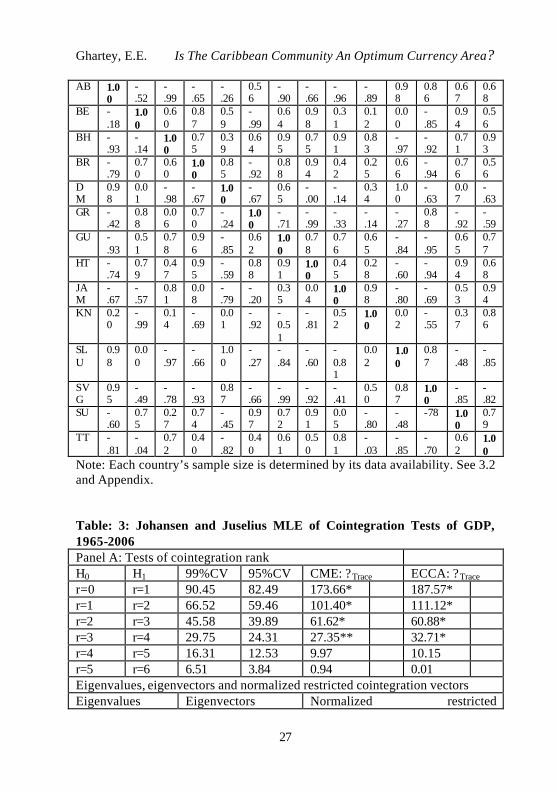
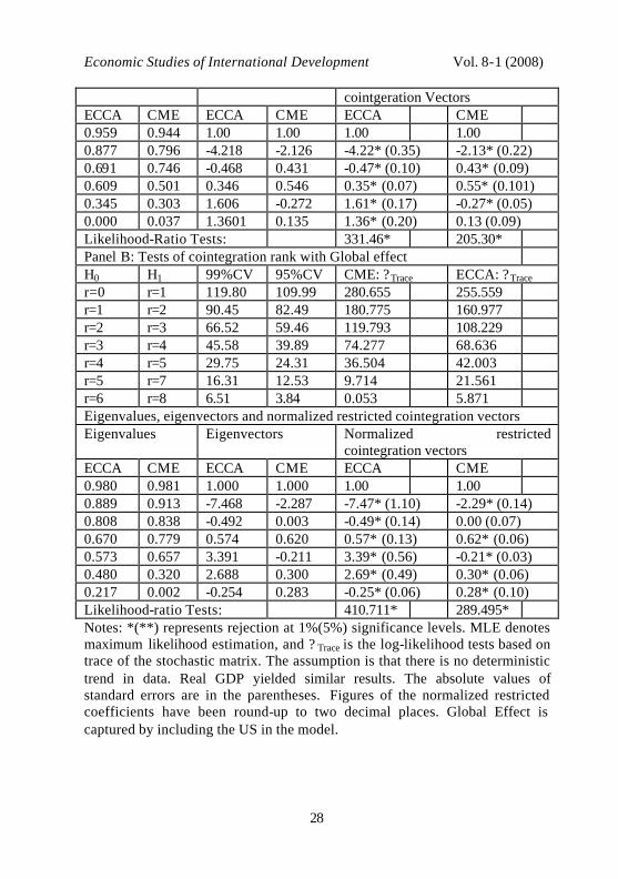
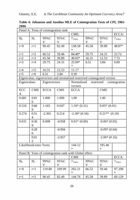
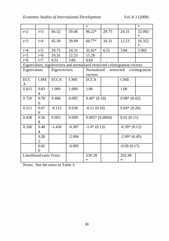
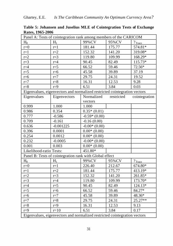
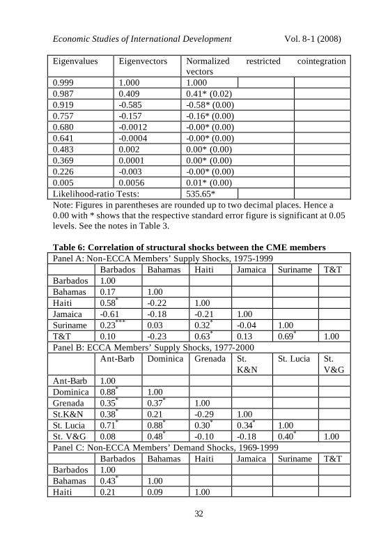
and 88 to 100 percent for real income, although they are asymmetric for several members. 4.2: Multivariate cointegration analysis To test for the OCA criteria by using symmetry of shocks, we have employed the VECM which requires cointegration to serve as an identifying restriction to reduce the computation and simplify the transformation of the system. The Johansen and Juselius (1993) maximum likelihood estimation of cointegration tests of output, prices and exchange rate are reported in Tables 3-5, respectively. The cointegration rank of output is four for both ECCA and non ECCA members at 0.05 significant levels. Thus, there are at most four cointegration vectors and two independent common stochastic trends for output among members. However, when global influences are introduced by including the US, the cointegration vectors increase to five for the non ECCA members and six for the ECCA members at 0.05 significant levels. See Table 3. In Table 4, there are at most four cointegration vectors for prices among the non ECCA members at 0.05 significant levels, and at most one cointegration vector among the ECCA members at 0.01 significant levels. With exposure to global influences, the cointegration vectors increase to at most five for the non ECCA members and four for the ECCA members. This shows that there are two independent common trends for prices among the non ECCA members and three for the ECCA members. The number of cointegration vectors increases to at most five for the non ECCA members, and four for the ECCA members when global influences are captured by including the US. Thus despite global influence, the number of independent common trends for prices remains to be two for the non ECCA members but drops to one for the ECCA members. In Table 5, there are at most five cointegration vectors for exchange rate for the entire CME members at 0.05 significant levels with four common stochastic trends for exchange rates. However, with global effect, the cointegration vectors increase to at most eight at 0.05 significant levels, leaving two common stochastic trends. Note that the ECCA members use a single currency, the ECCA dollar. The relative strength of the cointegration relationship among the members is very robust and can be assessed by the magnitudes of


18

the eigenvalues. Evidently the cointegration vectors are highly correlated with the stationary component of the process. The leading normalized restricted cointegration vectors reported in Tables 3-5 are all significant as judged by their respective log-likelihood ratios. Estimates of the long-run coefficients of supply shocks in Table 3 reported as normalized restricted cointegration vectors are significant for three coefficients of the ECCA members and all the coefficients of the non ECCA members. Additionally, the significance of coefficients increases when global influences are included in the study.

In Panels A and B of Table 4, all the long-run coefficients of demand shocks from the normalized restricted cointegration results are significant with the exception of one coefficient which is found to be insignificant when global influences are included in the results. Monetary shocks in Table 5 have significant long-run coefficients for all CME members at 0.01 significant levels, even when global influences are accounted for by including the US. All of the countries5 in the results of Tables 3-5 are included in the VECM to estimate the impulse response functions for the shocks employed to test the OCA convergence criteria, namely: the correlation between members, relative sizes of those shocks and their speed of adjustment. 4.3: Correlation of Underlying Structural Shocks Bayoumi and Eichengreen (1992) note that in determining symmetry of shocks the correlation of real incomes is subject to conflated information. This is because an increase in real income can result from either an increase in supply shock (which is termed productivity shock in real business cycle theory) or from responses to demand shocks stemming from a world-wide boom or both. Thus a shock to real income is affected by both effects of shocks and responses. As a result, they adopted a VAR technique to decompose real income and prices into supply shocks, and demand shocks, respectively (see Blanchard and Quah’s, 1989).

Following (Lippi and Reichlin’s, 1994) comment on their approach, we have used a VECM which uses cointegration as an identifying restriction to decompose real income, prices and exchange rates into supply, demand and monetary shocks. Note that supply shocks are the ideal mechanism for investigating the feasibility of 5 See Table 2a for the list of countries included in the empirical analysis.


19

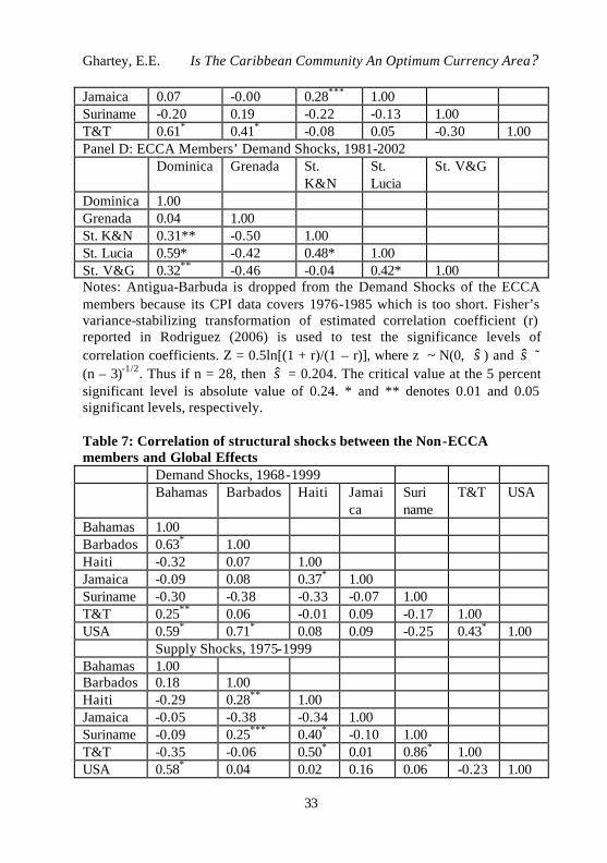
forming a monetary union by a group of economies, as it is less likely to include the effect of macroeconomic policy, unlike demand and monetary shocks which normally include the impact of macroeconomic policies being implemented (see Demertzis, et al. 2000). Correlations of supply shocks between non-ECCA members in Table 6 are negative with the exception of Barbados and Haiti, Suriname and Haiti, Trinidad-Tobago and Haiti, and Trinidad-Tobago and Suriname. Apart from Haiti and Suriname which are not Anglophone, it can be easily inferred that responsiveness of supply shocks between the non-ECCA members are generally asymmetric.

Correlations of supply shocks between members of the ECCA are significant in Panel B of Table 6. Only St. Kitts-Nevis and Grenada, Grenada and St. Vincent-Grenadines, and St. Kitts-Nevis and St. Vincent-Grenadines show asymmetric response to supply shocks, while St. Vincent-Grenadines and Antigua-Barbuda have insignificant response to supply shocks. This could be explained by the fact that their smaller sizes inhibit them from diversifying fully, which makes it difficult for them to effectively rely on a common monetary policy and their respective fiscal machinery to absorb supply shocks. Most ECCA members response to supply shocks are significant than the non-ECCA members. This can be explained by the fact the ECCA members share a common currency which imposes some discipline in their policy management, unlike the non ECCA members. The responsiveness to demand shocks in Panel C of Table 6 are also asymmetric between most non-ECCA members with the exception of Barbados and Bahamas, Trinidad-Tobago and Barbados, Bahamas and Trinidad-Tobago, and Jamaica and Haiti where demand shocks between them are significantly correlated.

Responses of demand shocks between the ECCA members are significant in Panel D of Table 6 despite the under sized sample of their prices. Only St. Vincent-Grenadines and St. Kitts-Nevis have asymmetric response to demand shocks. This shows that despite the benefits a common currency bestow on members, the administration of fiscal policies by each members can still influence their ability to effectively respond to demand shocks. In Table 7, when we include global effects, we find that demand shocks between most non-ECCA members are either


20

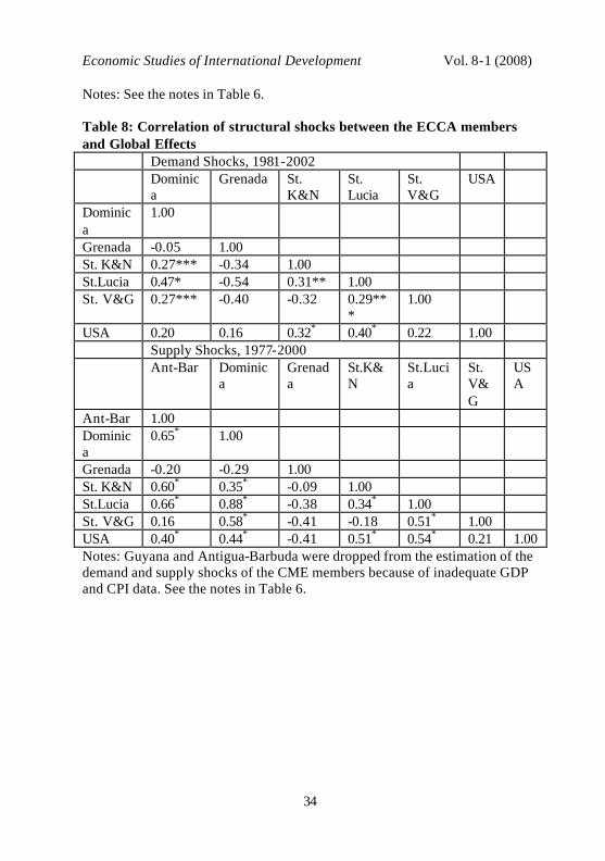
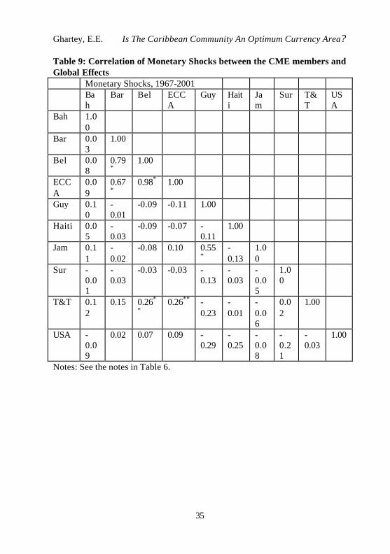
insignificant or asymmetric. Jamaica and Haiti, Trinidad-Tobago and The Bahamas, Barbados and The Bahamas have significant symmetric response to demand shocks. Additionally, shocks between The Bahamas and the USA, Barbados and the USA, and Trinidad-Tobago and the USA are highly significant than what prevail between the non-ECCA members. The rest of the non-ECCA members do not have symmetric response to demand shocks with the USA. Additiona lly, global effects of supply shocks in Table 7 show that only The Bahamas and USA are significantly correlated. This can be explained by the fact that The Bahamas maintains much closer ties with the US than with the CME members. The Bahamian dollar is unofficially linked closely to the US dollar and that is why it is hesitant to become a full-fledge member of the CME. We also find significant symmetric response to supply shocks between Barbados and Haiti, Barbados and Suriname, Trinidad-Tobago and Haiti, and Trinidad-Tobago and Suriname. This suggests that only they are more likely to succeed in adopting a common currency to employ a common monetary policy to deal with adverse supply shocks. The rest of non-ECCA members have either asymmetric or insignificant response to supply shocks between them in the face of global influence. In Table 9, correlations of monetary shocks between the non-ECCA members are even less promising. Belize and Barbados, Belize and ECCA members, Barbados and ECCA members, Trinidad-Tobago and ECCA members, and Jamaica and Guyana show highly significant correlations. The rest of the countries do not show any significant correlations between members. This suggests that Barbados, Belize and Trinidad-Tobago can be considered as potential candidates to join the ECCA members to form an OCA, since they can employ a common monetary and exchange rate policy to respond to monetary shocks, although the inflation rates of Belize require a special attention. The results are strengthened when the ECCA members are exposed to global effects (Bayoumi and Eichengreen, 1992) in the face of only demand shocks in Table 8. With the exception of Grenada which shows asymmetric response to demand shocks with the rest of members, and St. Vincent-Grenadines and St. Kitts-Nevis which have insignificant correlation between them; responses to demand shocks between the remaining ECCA members are highly significant.


21

The responsiveness to supply shocks between the ECCA members are also highly significant in Table 8, except again, Grenada which shows asymmetric response with other ECCA members and the USA. It is safe to conclude from the empirical evidence that both demand and supply shocks between the ECCA members are highly and significantly correlated because they share a common currency. 4.2.1: Relative Sizes and Speed of Adjustment to Shocks

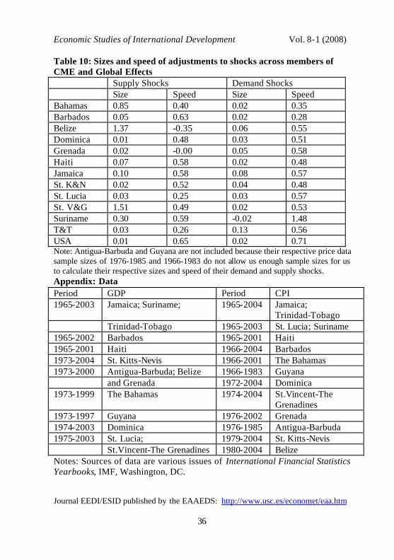
In Table 10, results of relative sizes of underlying structural demand and supply shocks of the CME members are measured by one-year (or four quarters) responsiveness from a unit demand shock, and five-year responsiveness from a unit supply shock. Note that a larger size of underlying shock definitely means that a member will be better served by adopting a flexible exchange rate to pursue independent policy in response to shocks, than joining a common currency or a fixed exchange rate regime to respond to such shocks.

The speed of adjustments and sizes of shocks by (Bayoumi and Eichengreen, 1992) were also employed by (Zhang, et al. 2004). The concept is very subjective as it is determined by the researcher who takes into account the characteristics of the economy and the type of data available. Bayoumi and Eichengreen (1992) use three years impulse response as a ratio of the long-run to measure speed of adjustment to supply shocks for the US, and (Zhang, et al. 2004) use four-quarters (or a year) response as a ratio of long-run effect of 20-quarter (or five-year) horizon. Considering that our annual data is affected by under-sized sample problem, the speed of adjustment to demand shocks is measured by the response after one-year as a share of the long-run effect which is measured by the sum of responses after second-year to the end of the period. 6

The speed of adjustment to supply shocks is measured by the response of five-year to a unit shock as a share of the long-run effect which is measured by the sum of responses after the fifth-year to the end of the horizon similar to (Zhang, et al. 2004).7 This naturally means

6 Note that because sizes of shocks are arbitrary, (Zhang, et al. 2004, fn18.) use the one-quarter impact in calculating the size of demand and monetary shocks. 7 Bayoumi and Eichengreen (1992, p.33) cite the simple measure of the speed of adjustment to shocks as the ratio of the impulse response function in the


22

that our speed will be much slower compared with previous studies. We have applied the method consistently across the board for reliable results. Note again, that for the CME members, it is plausible to even use longer shocks than what we have used in the calculation as it will take much longer time for such shocks to taper off because of structural bottlenecks since communications and infrastructure are not as well developed as the US, our ideal OCA. Nevertheless, it could also be argued that because most members of the CME are small island economies, the time it takes for their shocks to wear off may not be longer than the US which spans a much larger area with a much larger population.

Results of Table 10 show that apart from Belize, St. Vincent-Grenadines, and The Bahamas, which experience relatively large supply shocks unaccompanied by faster speed of adjustment, Suriname experiences moderately large shock with relatively faster speed of adjustment. Jamaica experiences 10 percent supply shocks but its speed of adjustment is about 57 percent, which is more than the average speed. The rest of the countries experience fairly normal supply shocks with sizes that are less than 10 percent. Dominica has the same size of supply shocks as the US but its speed of adjustment of 48 percent is less than the median speed of adjustment in our study. Barbados experiences almost the same speed of adjustment as the US, although the latter has a smaller size of supply shocks. Grenada experiences a smaller size of supply shocks but its speed of adjustment to those shocks is extremely slow, almost zero.

Sizes of demand shocks among members in Table 10 are comparable to that of the US, but whereas the speed of adjustment to such shocks is very high in the US, most CME members have moderate speed of adjustments. The Bahamas, Barbados, Haiti and St. Kitts-Nevis have speed of adjustments which are less than the average speed of 50 percent. Suriname has the fastest speed of adjustments to demand shocks in the study but its size is negative or asymmetric so it is not easy to explain its relevance. With the exception of St. Lucia, the rest of ECCA members experience more than average speed of adjustment third-year to its long-run level. A higher ratio indicates a faster speed of adjustment to shocks and a lower ratio shows a slower speed of adjustment to shocks.


23

to demand shocks. On the average, with a global effect, of the 4 percent demand shocks experienced in the region about 67 percent adjustment is completed within a year; whereas the US experience 2 percent shocks and completes 71 percent of the adjustment within a year.

Thus, we can surmise that the relatively large size of shocks and slow speed of adjustment in the Caribbean compared with the US are due to the relatively inflexible labor market and rigid wage rates in the region where activities of the numerous unions render internal adjustments to shocks rather difficult. 5: Conclusion The empirical findings show that the ECCA members experience significantly higher correlation between them than the non-ECCA members. Speed of adjustment to demand shocks are not distinctly different from the ECCA and non-ECCA members, but supply shocks of the ECCA members are relatively faster than the non-ECCA members. Additionally, sizes of the ECCA members’ demand and supply shocks are relatively smaller than the normal experience of the non-ECCA members with the exception of St. Vincent and the Grenadines. The results also lend credence to the fact that using a common currency bestows on members some OCA benefits which can only grow with time, as structural shocks of the ECCA members are more symmetrical than the non-ECCA members who practice independent monetary policy. Monetary shocks results suggest that Barbados, Belize and Trinidad-Tobago could join the ECCA to form an OCA in the region, although supply and demand shocks with global effects show that Belize and Trinidad-Tobago will be poor candidates. Additionally, the US being a well diversified economy which can be considered as an OCA, has a relatively smaller size of shocks and faster speed of adjustment to shocks than the CME members; therefore adopting a common currency may not be a smooth sail for the CME members.


24

Bibliography Bayoumi, T. and B. Eichengreen (1992), “Shocking Aspects of European Monetary Unification,” NBER, Working Paper No. 3949: 1-39. Bean, C.R. (1992), “Economic and monetary union in Europe,” Journal of Economic Perspectives, 6(4): 31-52. Blanchard, O.J. and D. Quah (1989), “The Dynamic Effects of Aggregate Supply and Demand Disturbances,” American Economics Review, 79: 655-673. Demertzis, M., A.H. Hallet and O. Rummel (2000), “Is the European Union a National Currency Area, or is it held together by Policy Makers?” Weltwirtschaftliches Archiv , 135: 657-679. Fleming, J.M. (1971), “On exchange rate unification,” Economic Journal, 81: 467-488. Frankel, J.A., and A.K. Rose (2000), “Estimating the effect of currency unions on trade and output,” NBER Working Paper 7857, August. _____ and _____ (1998), “The endogeneity of optimum currency area criteria,” Economic Journal, 108: 1009-1025. Ghartey, E.E. (2003), “Monetary policy and deficits financing in Jamaica,” Journal of Economic Development, 28 (1): 81-99. Grubel, H. (1970), “The Theory of Optimum Currency Area,” Canadian Journal of Economics, 3 (2): 318-324. Johansen, S. and K. Juselius (1993), “Testing structural hypothesis in a multivariate cointegration analysis of the PPP and the UIP for the UK,” Journal of Econometrics, 53: 211-244. Kenen, P.B. (1969), “The theory of optimum currency areas: an eclectic view,” in Monetary problems of the international economy , R.A. Mundell and A.K. Swoboda (eds.) (Chicago: University of Chicago Press), 41-60. _____ (1997), “Common currencies versus currency areas,” American Economic Review, 87(2): 211-213. Lippi, M. and L. Reichlin (1993), “The Dynamic Effects of Aggregate Demand and Supply Disturbances: Comment,” American Economic Review, 83 (3): 644-652. Manioc, O. and J.G. Montauban (2001), “Is a monetary union in CARICOM desirable?” LEAD, University of Antilles and Guyana. McKinnon, R.I. (1963), “Optimum currency areas,” American Economic Review, 53: 717-25.


25

Mundell, R.A. (1961), “Theory of optimum currency areas,” American Economic Review, 51: 657-665. Nitsch, V. (2002), “Honey, I shrunk the currency union effect on trade,” The World Economy , 25(4): 457-474. Parkin, M. (1972), “An overwhelming case for European Monetary Union,” Banker, 122: 1139-1142. Rodriguez, R.N. (2006), “Correlation,” Encyclopedia of Statistical Sciences, Wiley-Inter-Science, 2: 1375-1385. Rose, A.K. (2000), “One money one market,” Economic Policy, 15-30: 7-46. _____ and C. Engel (2000), “Currency union and international integration,” NBER Working Paper 7872, September. Summary, R.M. (1989), “A Political-Economic Model of US Bilateral Trade,” Review of Economics and Statistics, 71 (1): 179-182. Tavlas, G.S. (1993), “The ‘new’ theory of optimum currency areas,” World Economy , 16: 663-685. Zhang, Z., K. Sato and M. McAleer (2004), “Is a Monetary Union Feasible for East Asia?” Applied Economics, 36: 1031-1043. Table 2a: Standard deviations and correlations of inflation and real economic growth Std. dev. Of

Inflation Correlation of Inflation

Std. Dev. Of Economic Growth

Correlation of Economic Growth

Ant. & Barb 0.06 0.97 1.00 0.08 0.32 1.00 Bahamas 1.43 0.99 0.99 0.07 -0.01 0.37 Barbados 0.06 0.99 0.91 0.09 0.94 0.27 Belize 2.07 0.99 0.99 0.09 0.41 0.31 Dominica 0.06 0.91 0.98 0.08 0.29 0.57 Grenada 0.06 0.95 1.00 0.81 -0.22 -0.45 Guyana 0.06 0.89 0.74 0.22 0.99 -0.22 Haiti 0.09 0.12 0.37 0.10 0.27 -0.18 Jamaica 0.12 -0.90 -0.76 0.10 -0.66 -0.34 St. K & N 0.03 1.00 0.96 0.05 -0.26 0.38 St. Lucia 0.08 0.88 0.97 0.08 0.44 0.70 St. V & G 2.12 0.98 1.00 0.06 -0.88 0.29 Suriname 0.35 0.90 0.98 0.35 -0.46 -0.30 T & T 0.04 -0.16 0.09 0.11 -0.99 0.24 USA 0.03 1.00 0.97 0.02 1.00 0.34


26

Table 2b: Correlation of Economic Growth, Inflation, and Real Income between the CME members Economic Growth(Lower Triangular matrix)\ Inflation(Upper triangular matrix) A

B BE B

H BR

DM

GR

GU

HT

JAM

SKN

SLU

SVG

SU TT

AB 1.00

0.99

0.99

0.91

0.98

1.00

0.74

0.37

-0.76

0.96

0.97

1.00

0.98

0.09

BE 0.31

1.00

1.00

0.96

0.96

0.99

0.82

0.25

-0.83

0.99

0.94

1.00

0.95

-.03

BH 0.37

0.32

1.00

0.96

0.95

0.98

0.82

0.24

-0.83

0.99

0.93

1.00

0.95

-.04

BR 0.27

0.20

0.33

1.00

0.83

0.90

0.95

-.04

-0.95

0.99

0.80

0.94

0.82

-.32

DM

0.57

-.19

0.05

0.06

1.00

0.99

0.61

0.52

-0.63

0.90

1.00

0.97

1.00

0.26

GR -0.45

-.23

-0.18

-.44

-.57

1.00

0.71

0.41

-0.73

0.95

0.98

0.99

0.99

0.13

GU -0.22

0.08

-0.20

-.22

-.20

0.48

1.00

-.35

-1.00

0.90

0.57

0.78

0.60

-.60

HT -0.18

-.31

-0.15

0.09

-.10

0.19

-0.10

1.00

0.33

0.09

0.57

0.31

0.54

0.96

JAM

-0.34

0.00

-0.43

-.55

-.31

0.52

0.44

0.01

1.00

-0.91

-.59

-.79

-.62

0.58

SKN

0.38

0.01

0.29

0.44

0.17

-.04

0.02

-.19

-0.03

1.00

0.87

0.97

0.89

-.19

SLU

0.70

0.40

0.43

0.24

0.65

-.73

-0.23

-.23

-0.37

0.15

1.00

0.96

1.00

0.32

SVG

0.29

0.31

0.35

0.26

0.45

-.77

-0.37

-.57

-0.42

0.16

0.64

1.00

0.97

0.03

SU -0.30

-.17

0.10

-.19

-.29

0.46

0.06

0.63

0.28

-0.18

-.35

-0.49

1.00

0.28

TT 0.24

-.03

0.05

0.49

0.31

-.43

-0.19

0.30

-0.35

0.06

0.36

0.21

0.15

1.00

Real Income (Lower Triangular matrix)\Real Per Capita Income (Upper Triangular matrix)


27

AB 1.00

-.52

-.99

-.65

-.26

0.56

-.90

-.66

-.96

-.89

0.98

0.86

0.67

0.68

BE -.18

1.00

0.60

0.87

0.59

-.99

0.64

0.98

0.31

0.12

0.00

-.85

0.94

0.56

BH -.93

-.14

1.00

0.75

0.39

0.64

0.95

0.75

0.91

0.83

-.97

-.92

0.71

0.93

BR -.79

0.70

0.60

1.00

0.85

-.92

0.88

0.94

0.42

0.25

0.66

-.94

0.76

0.56

DM

0.98

0.01

-.98

-.67

1.00

-.67

0.65

-.00

-.14

0.34

1.00

-.63

0.07

-.63

GR -.42

0.88

0.06

0.70

-.24

1.00

-.71

-.99

-.33

-.14

-.27

0.88

-.92

-.59

GU -.93

0.51

0.78

0.96

-.85

0.62

1.00

0.78

0.76

0.65

-.84

-.95

0.65

0.77

HT -.74

0.79

0.47

0.95

-.59

0.88

0.91

1.00

0.45

0.28

-.60

-.94

0.94

0.68

JAM

-.67

-.57

0.81

0.08

-.79

-.20

0.35

0.04

1.00

0.98

-.80

-.69

0.53

0.94

KN 0.20

-.99

0.14

-.69

0.01

-.92

-0.51

-.81

0.52

1.00

0.02

-.55

0.37

0.86

SLU

0.98

0.00

-.97

-.66

1.00

-.27

-.84

-.60

-0.81

0.02

1.00

0.87

-.48

-.85

SVG

0.95

-.49

-.78

-.93

0.87

-.66

-.99

-.92

-.41

0.50

0.87

1.00

-.85

-.82

SU -.60

0.75

0.27

0.74

-.45

0.97

0.72

0.91

0.05

-.80

-.48

-78 1.00

0.79

TT -.81

-.04

0.72

0.40

-.82

0.40

0.61

0.50

0.81

-.03

-.85

-.70

0.62

1.00

Note: Each country’s sample size is determined by its data availability. See 3.2 and Appendix. Table: 3: Johansen and Juselius MLE of Cointegration Tests of GDP, 1965-2006 Panel A: Tests of cointegration rank H0 H1 99%CV 95%CV CME: ?Trace ECCA: ?Trace r=0 r=1 90.45 82.49 173.66* 187.57* r=1 r=2 66.52 59.46 101.40* 111.12* r=2 r=3 45.58 39.89 61.62* 60.88* r=3 r=4 29.75 24.31 27.35** 32.71* r=4 r=5 16.31 12.53 9.97 10.15 r=5 r=6 6.51 3.84 0.94 0.01 Eigenvalues, eigenvectors and normalized restricted cointegration vectors Eigenvalues Eigenvectors Normalized restricted


28

cointgeration Vectors ECCA CME ECCA CME ECCA CME 0.959 0.944 1.00 1.00 1.00 1.00 0.877 0.796 -4.218 -2.126 -4.22* (0.35) -2.13* (0.22) 0.691 0.746 -0.468 0.431 -0.47* (0.10) 0.43* (0.09) 0.609 0.501 0.346 0.546 0.35* (0.07) 0.55* (0.101) 0.345 0.303 1.606 -0.272 1.61* (0.17) -0.27* (0.05) 0.000 0.037 1.3601 0.135 1.36* (0.20) 0.13 (0.09) Likelihood-Ratio Tests: 331.46* 205.30* Panel B: Tests of cointegration rank with Global effect H0 H1 99%CV 95%CV CME: ?Trace ECCA: ?Trace r=0 r=1 119.80 109.99 280.655 255.559 r=1 r=2 90.45 82.49 180.775 160.977 r=2 r=3 66.52 59.46 119.793 108.229 r=3 r=4 45.58 39.89 74.277 68.636 r=4 r=5 29.75 24.31 36.504 42.003 r=5 r=7 16.31 12.53 9.714 21.561 r=6 r=8 6.51 3.84 0.053 5.871 Eigenvalues, eigenvectors and normalized restricted cointegration vectors Eigenvalues Eigenvectors Normalized restricted

cointegration vectors ECCA CME ECCA CME ECCA CME 0.980 0.981 1.000 1.000 1.00 1.00 0.889 0.913 -7.468 -2.287 -7.47* (1.10) -2.29* (0.14) 0.808 0.838 -0.492 0.003 -0.49* (0.14) 0.00 (0.07) 0.670 0.779 0.574 0.620 0.57* (0.13) 0.62* (0.06) 0.573 0.657 3.391 -0.211 3.39* (0.56) -0.21* (0.03) 0.480 0.320 2.688 0.300 2.69* (0.49) 0.30* (0.06) 0.217 0.002 -0.254 0.283 -0.25* (0.06) 0.28* (0.10) Likelihood-ratio Tests: 410.711* 289.495* Notes: *(**) represents rejection at 1%(5%) significance levels. MLE denotes maximum likelihood estimation, and ? Trace is the log-likelihood tests based on trace of the stochastic matrix. The assumption is that there is no deterministic trend in data. Real GDP yielded similar results. The absolute values of standard errors are in the parentheses. Figures of the normalized restricted coefficients have been round-up to two decimal places. Global Effect is captured by including the US in the model.


29

Table 4: Johansen and Juselius MLE of Cointegration Tests of CPI, 1965-2006 Panel A: Tests of cointegration rank CME: ECCA: H0 H1 99%C

V 95%CV

?Trace 99%CV

95%CV

?Trace

r=0 r=1 90.45 82.49 138.58*

45.58 39.89 48.87*

r=1 r=2 66.52 59.46 84.40* 29.75 24.31 23.72 r=2 r=3 45.58 39.89 49.03* 16.31 12.53 7.73 r=3 r=4 29.75 24.31 25.94*

* 6.51 3.84 0.69

r=4 r=5 16.31 12.53 11.17 r=5 r=6 6.51 3.84 0.39 Eigenvalue, eigenvectors and normalized restricted cointegrated vectors Eigenvalues Eigenvectors Normalized restricted cointegration

vectors ECCA

CME ECCA CME ECCA CME

0.681 0.816

1.000 1.000 1.00 1.00

0.516 0.669

1.165 0.047 1.16* (0.31) 0.05* (0.01)

0.274 0.514

-2.365 0.214 -2.36* (0.34) 0.21** (0.10)

0.031 0.369

0.008 -0.058 0.01* (0.00) -0.06* (0.05)

0.286

-0.094 -0.09* (0.04)

0.012

-2.057 -2.06* (0.16)

Likelihood-ratio Tests: 144.12*

185.46*

Panel B: Tests of cointegration rank with Global effect CME ECCA H0 H1 99%C

V 95%CV

?Trace 99%CV

95%CV

?Trace

r=0 r=1 119.80 109.99 202.21*

66.52 59.46 97.298*

r=1 r=2 90.45 82.49 144.76 45.58 39.89 60.129


30

* * r=2 r=3 66.52 59.46 96.22* 29.75 24.31 32.082

* r=3 r=4 45.58 39.89 60.77* 16.31 12.53 16.352

* r=4 r=5 29.75 24.31 32.41* 6.51 3.84 3.985 r=5 r=6 16.31 12.53 11.26 r=6 r=7 6.51 3.84 0.64 Eigenvalues, eigenvectors and normalized restricted cointegration vectors Eigenvalues Eigenvectors Normalized restricted cointegration

vectors ECCA

CME ECCA CME ECCA CME

0.815 0.834

1.000 1.000 1.00 1.00

0.720 0.780

0.466 0.085 0.46* (0.10) 0.08* (0.02)

0.511 0.670

-0.112 0.636 -0.11 (0.16) 0.64* (0.26)

0.430 0.588

0.005 0.009 0.005* (0.0004) 0.01 (0.11)

0.166 0.484

-1.430 -0.387 -1.4* (0.13) -0.39* (0.12)

0.282

-2.994 -2.99* (0.45)

0.020

-0.093 -0.09 (0.17)

Likelihood-ratio Tests: 230.39*

292.49*

Notes: See the notes in Table 3.


31

Table 5: Johansen and Juselius MLE of Cointegration Tests of Exchange Rates, 1965-2006 Panel A: Tests of cointegration rank among members of the CARICOM H0 H1 99%CV 95%CV ?Trace r=0 r=1 181.44 175.77 574.81* r=1 r=2 152.32 141.20 319.08* r=2 r=3 119.80 109.99 168.29* r=3 r=4 90.45 82.49 115.73* r=4 r=5 66.52 59.46 72.56* r=5 r=6 45.58 39.89 37.19 r=6 r=7 29.75 24.31 19.52 r=7 r=8 16.31 12.53 9.28 r=8 r=9 6.51 3.84 0.03 Eigenvalues, eigenvectors and normalized restricted cointegration vectors Eigenvalues Eigenvectors Normalized restricted cointegration

vectors 0.999 1.000 1.000 0.986 0.354 0.35* (0.01) 0.777 -0.586 -0.59* (0.00) 0.709 -0.161 -0.16 (0.00) 0.636 -0.001225 -0.00* (0.00) 0.396 0.0001 0.00* (0.00) 0.254 0.0012 0.00* (0.00) 0.232 -0.0005 -0.00* (0.00) 0.001 0.003 0.00* (0.00) Likelihood-ratio Tests: 451.80* Panel B: Tests of cointegration rank with Global effect H0 H1 99%CV 95%CV ?Trace r=0 r=1 226.40 212.67 674.80* r=1 r=2 181.44 175.77 413.19* r=2 r=3 152.32 141.20 261.85* r=3 r=4 119.80 109.99 173.70* r=4 r=5 90.45 82.49 124.13* r=5 r=6 66.52 59.46 84.27* r=6 r=7 45.58 39.89 48.36* r=7 r=8 29.75 24.31 25.27** r=8 r=9 16.31 12.53 9.13 r=9 r=10 6.51 3.84 0.17 Eigenvalues, eigenvectors and normalized restricted cointegration vectors


32

Eigenvalues Eigenvectors Normalized restricted cointegration vectors

0.999 1.000 1.000 0.987 0.409 0.41* (0.02) 0.919 -0.585 -0.58* (0.00) 0.757 -0.157 -0.16* (0.00) 0.680 -0.0012 -0.00* (0.00) 0.641 -0.0004 -0.00* (0.00) 0.483 0.002 0.00* (0.00) 0.369 0.0001 0.00* (0.00) 0.226 -0.003 -0.00* (0.00) 0.005 0.0056 0.01* (0.00) Likelihood-ratio Tests: 535.65* Note: Figures in parentheses are rounded up to two decimal places. Hence a 0.00 with * shows that the respective standard error figure is significant at 0.05 levels. See the notes in Table 3. Table 6: Correlation of structural shocks between the CME members Panel A: Non-ECCA Members’ Supply Shocks, 1975-1999 Barbados Bahamas Haiti Jamaica Suriname T&T Barbados 1.00 Bahamas 0.17 1.00 Haiti 0.58* -0.22 1.00 Jamaica -0.61 -0.18 -0.21 1.00 Suriname 0.23*** 0.03 0.32* -0.04 1.00 T&T 0.10 -0.23 0.63* 0.13 0.69* 1.00 Panel B: ECCA Members’ Supply Shocks, 1977-2000 Ant-Barb Dominica Grenada St.

K&N St. Lucia St.

V&G Ant-Barb 1.00 Dominica 0.88* 1.00 Grenada 0.35* 0.37* 1.00 St.K&N 0.38* 0.21 -0.29 1.00 St. Lucia 0.71* 0.88* 0.30* 0.34* 1.00 St. V&G 0.08 0.48* -0.10 -0.18 0.40* 1.00 Panel C: Non-ECCA Members’ Demand Shocks, 1969-1999 Barbados Bahamas Haiti Jamaica Suriname T&T Barbados 1.00 Bahamas 0.43* 1.00 Haiti 0.21 0.09 1.00


33

Jamaica 0.07 -0.00 0.28*** 1.00 Suriname -0.20 0.19 -0.22 -0.13 1.00 T&T 0.61* 0.41* -0.08 0.05 -0.30 1.00 Panel D: ECCA Members’ Demand Shocks, 1981-2002 Dominica Grenada St.

K&N St. Lucia

St. V&G

Dominica 1.00 Grenada 0.04 1.00 St. K&N 0.31** -0.50 1.00 St. Lucia 0.59* -0.42 0.48* 1.00 St. V&G 0.32** -0.46 -0.04 0.42* 1.00 Notes: Antigua-Barbuda is dropped from the Demand Shocks of the ECCA members because its CPI data covers 1976-1985 which is too short. Fisher’s variance-stabilizing transformation of estimated correlation coefficient (r) reported in Rodriguez (2006) is used to test the significance levels of correlation coefficients. Z = 0.5ln[(1 + r)/(1 – r)], where z ~ N(0, s ) and s ˜ (n – 3)-1/2. Thus if n = 28, then s = 0.204. The critical value at the 5 percent significant level is absolute value of 0.24. * and ** denotes 0.01 and 0.05 significant levels, respectively. Table 7: Correlation of structural shocks between the Non-ECCA members and Global Effects Demand Shocks, 1968-1999 Bahamas Barbados Haiti Jamai

ca Suri name

T&T USA

Bahamas 1.00 Barbados 0.63* 1.00 Haiti -0.32 0.07 1.00 Jamaica -0.09 0.08 0.37* 1.00 Suriname -0.30 -0.38 -0.33 -0.07 1.00 T&T 0.25** 0.06 -0.01 0.09 -0.17 1.00 USA 0.59* 0.71* 0.08 0.09 -0.25 0.43* 1.00 Supply Shocks, 1975-1999 Bahamas 1.00 Barbados 0.18 1.00 Haiti -0.29 0.28** 1.00 Jamaica -0.05 -0.38 -0.34 1.00 Suriname -0.09 0.25*** 0.40* -0.10 1.00 T&T -0.35 -0.06 0.50* 0.01 0.86* 1.00 USA 0.58* 0.04 0.02 0.16 0.06 -0.23 1.00


34

Notes: See the notes in Table 6. Table 8: Correlation of structural shocks between the ECCA members and Global Effects Demand Shocks, 1981-2002 Dominic

a Grenada St.

K&N St. Lucia

St. V&G

USA

Dominica

1.00

Grenada -0.05 1.00 St. K&N 0.27*** -0.34 1.00 St.Lucia 0.47* -0.54 0.31** 1.00 St. V&G 0.27*** -0.40 -0.32 0.29**

* 1.00

USA 0.20 0.16 0.32* 0.40* 0.22 1.00 Supply Shocks, 1977-2000 Ant-Bar Dominic

a Grenada

St.K&N

St.Lucia

St. V&G

USA

Ant-Bar 1.00 Dominica

0.65* 1.00

Grenada -0.20 -0.29 1.00 St. K&N 0.60* 0.35* -0.09 1.00 St.Lucia 0.66* 0.88* -0.38 0.34* 1.00 St. V&G 0.16 0.58* -0.41 -0.18 0.51* 1.00 USA 0.40* 0.44* -0.41 0.51* 0.54* 0.21 1.00 Notes: Guyana and Antigua-Barbuda were dropped from the estimation of the demand and supply shocks of the CME members because of inadequate GDP and CPI data. See the notes in Table 6.


35

Table 9: Correlation of Monetary Shocks between the CME members and Global Effects Monetary Shocks, 1967-2001 Ba

h Bar Bel ECC

A Guy Hait

i Jam

Sur T&T

USA

Bah 1.00

Bar 0.03

1.00

Bel 0.08

0.79*

1.00

ECCA

0.09

0.67*

0.98* 1.00

Guy 0.10

-0.01

-0.09 -0.11 1.00

Haiti 0.05

-0.03

-0.09 -0.07 -0.11

1.00

Jam 0.11

-0.02

-0.08 0.10 0.55*

-0.13

1.00

Sur -0.01

-0.03

-0.03 -0.03 -0.13

-0.03

-0.05

1.00

T&T 0.12

0.15 0.26*

* 0.26** -

0.23 -0.01

-0.06

0.02

1.00

USA -0.09

0.02 0.07 0.09 -0.29

-0.25

-0.08

-0.21

-0.03

1.00

Notes: See the notes in Table 6.


36

Table 10: Sizes and speed of adjustments to shocks across members of CME and Global Effects Supply Shocks Demand Shocks Size Speed Size Speed Bahamas 0.85 0.40 0.02 0.35 Barbados 0.05 0.63 0.02 0.28 Belize 1.37 -0.35 0.06 0.55 Dominica 0.01 0.48 0.03 0.51 Grenada 0.02 -0.00 0.05 0.58 Haiti 0.07 0.58 0.02 0.48 Jamaica 0.10 0.58 0.08 0.57 St. K&N 0.02 0.52 0.04 0.48 St. Lucia 0.03 0.25 0.03 0.57 St. V&G 1.51 0.49 0.02 0.53 Suriname 0.30 0.59 -0.02 1.48 T&T 0.03 0.26 0.13 0.56 USA 0.01 0.65 0.02 0.71 Note: Antigua-Barbuda and Guyana are not included because their respective price data sample sizes of 1976-1985 and 1966-1983 do not allow us enough sample sizes for us to calculate their respective sizes and speed of their demand and supply shocks. Appendix: Data Period GDP Period CPI 1965-2003 Jamaica; Suriname; 1965-2004 Jamaica;

Trinidad-Tobago Trinidad-Tobago 1965-2003 St. Lucia; Suriname 1965-2002 Barbados 1965-2001 Haiti 1965-2001 Haiti 1966-2004 Barbados 1973-2004 St. Kitts-Nevis 1966-2001 The Bahamas 1973-2000 Antigua-Barbuda; Belize 1966-1983 Guyana and Grenada 1972-2004 Dominica 1973-1999 The Bahamas 1974-2004 St.Vincent-The

Grenadines 1973-1997 Guyana 1976-2002 Grenada 1974-2003 Dominica 1976-1985 Antigua-Barbuda 1975-2003 St. Lucia; 1979-2004 St. Kitts-Nevis St.Vincent-The Grenadines 1980-2004 Belize Notes: Sources of data are various issues of International Financial Statistics Yearbooks, IMF, Washington, DC. Journal EEDI/ESID published by the EAAEDS: http://www.usc.es/economet/eaa.htm

Documents

IS THE CARIBBEAN COMMUNITY AN OPTIMUM … Studies of International Development Vol. 8-1 (2008) IS THE CARIBBEAN COMMUNITY AN OPTIMUM CURRENCY AREA? GHARTEY, Edward E.* Abstract This