Embed Size (px)
Citation preview

IRT Models to Assess Change Across Repeated Measurements
James S. RobertsGeorgia Institute of Technology
Qianli MaUniversity of Maryland
University of Maryland
Many Thanks!!!
• Thanks Bob.
• Thanks to Mayank Seksaria,Vallerie Ellis, Dan Graham, Yi Cao, and Yunyun Dai for their assistance at various stages of this project.
• Thanks to the Project MATCH Coordinating Center at the University of Connecticut for sharing their data.

Situations in Which Repeated Measures IRT Models Are Useful
• Each respondent receives the same test multiple times– Typical pretest, posttest, follow-up, treatment
studies
• Each respondent receives alternate forms of a comparable test with common items across forms (or across pairs of forms)– More elaborate repeated measures designs
that control for memory effects

• Each respondent receives alternate forms that are not comparable (in difficulty) but have some common items– Vertical measurement situations
• ECLS, Some school testing programs
• Each of these situations involves a set of common items across (successive pairs of) administered tests– 100% common items = same form– Less than 100% common items = alternate forms

Typical Approaches to Repeated Measures Data In IRT
• Calibrate responses from each administration separately– Ignores correlation of the latent trait across
test administrations
• Calibrate responses from each administration simultaneously allowing for different prior distributions at each administration– Still ignores correlation
• Multidimensional Approaches– Andersen (1985)– Reckase and Martineau (2004)– Estimate theta at each testing occasion
simultaneously
• Does incorporate correlation across testing occasions
• Does not really assess change in the latent variable

An Alternative IRT Approach
• Embretson’s (1991) Multidimensional Rasch Model for Learning and Change (MRMLC)
– Developed to measure change in a latent trait across repeatedly measured items that are scored as binary variables

)|1( **
,...,1)( TjjtijXP
)(
1
)(1
*
*
exp1
exp
ti
t
qqj
ti
t
qqj
b
b

Where: 11*
jj is the baseline (time 1) level of the latent trait for the jth respondent
122*
jjj is the change in the
level of latent trait from time1 to time 2for the jth respondent
)1(*
tjtjtj is the change in the
level of latent trait from time t -1 to time tfor the jth respondent with t = 2, …, T

bi(t) is the difficulty of the ith item nested within test administration t
There must be common itemsacross test form administrations andthe difficulty is assumed constant
for a given common item
This maintains the metricacross forms

• This model parameterizes the latent trait scores for each individual as an initial trait level followed by t-1 latent change scores
– It is multivariate in the sense that each individual has T latent trait scores
• However, each of these scores relates to positions on a single unidimensional continuum

Note that:
So the latent trait level for the jth individual at time t
(i.e., the composite trait at time t ) is the sum of the
initial level along with all the latent change scores
t
qjqjt
1
*

• Along with estimates of the aforementioned parameters, one also obtains estimates of the latent variable means and the correlation matrix for these latent variables:
**
2
*
1,...,,
T
TTTT
T
T
rrr
rrr
rrr
R
...
............
...
...
21
22221
11211
Advantages of the Multidimensional IRT Approach to Change
• Traditional Benefits of IRT Models that Fit the Data
– Sample invariant interpretation of item parameters
– Item invariant interpretation of person parameters
– Index of precision at the individual level
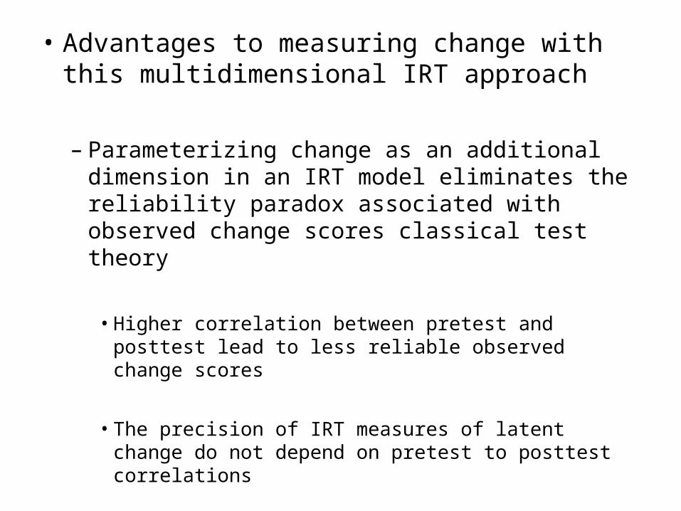
• Advantages to measuring change with this multidimensional IRT approach
– Parameterizing change as an additional dimension in an IRT model eliminates the reliability paradox associated with observed change scores classical test theory
• Higher correlation between pretest and posttest lead to less reliable observed change scores
• The precision of IRT measures of latent change do not depend on pretest to posttest correlations
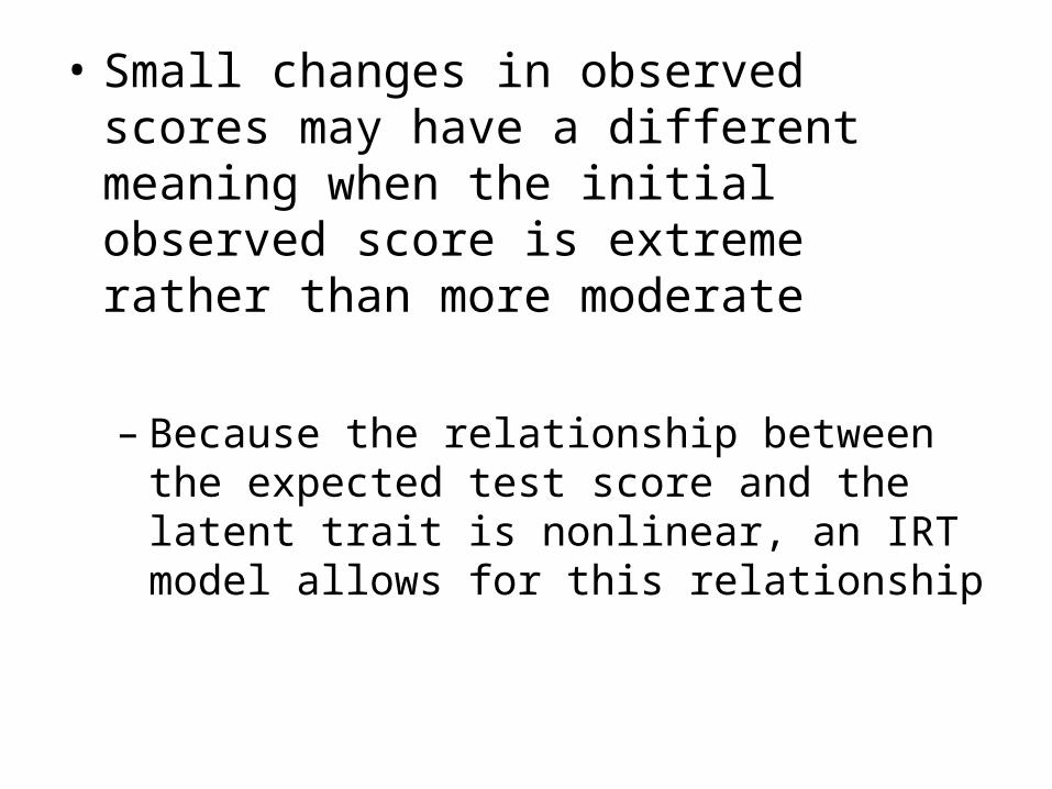
• Small changes in observed scores may have a different meaning when the initial observed score is extreme rather than more moderate
– Because the relationship between the expected test score and the latent trait is nonlinear, an IRT model allows for this relationship


Further Generalization of the Basic Model
• One can easily extend the MRMLC to more general situations
– Allow for graded (polytomous) responses
Wang, Wilson & Adams (1998)
Wang & Chyi-In (2004)
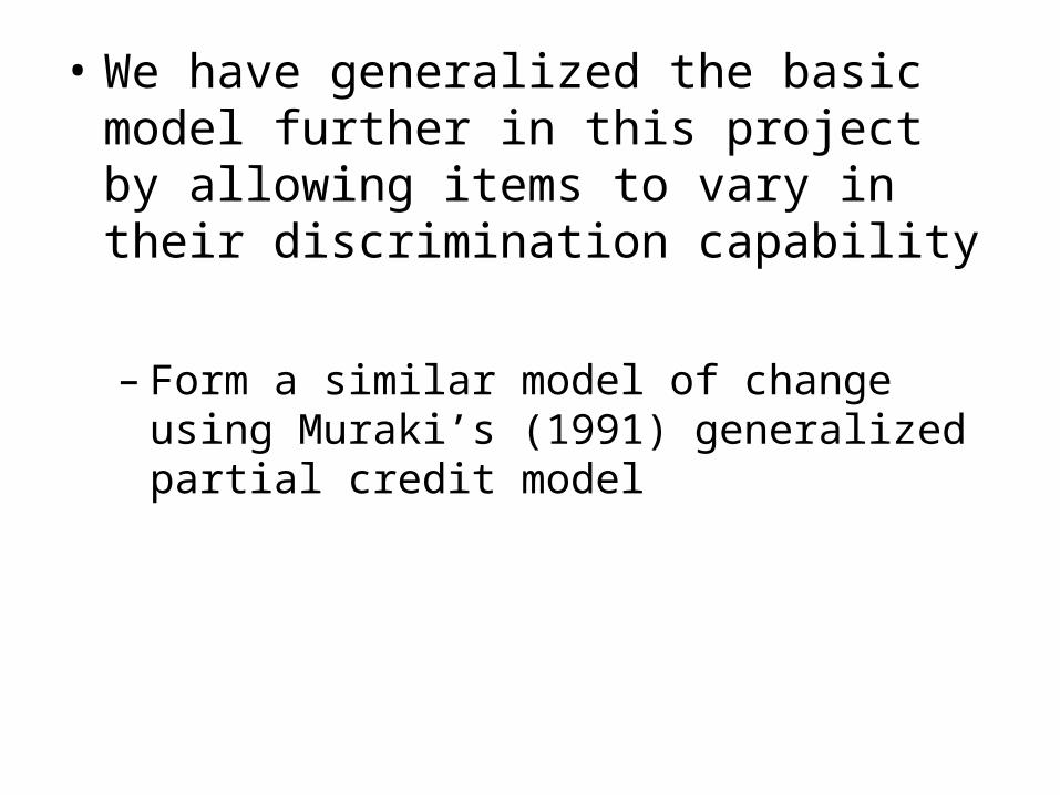
• We have generalized the basic model further in this project by allowing items to vary in their discrimination capability
– Form a similar model of change using Muraki’s (1991) generalized partial credit model

)|( **
,...,1)( Tjjtij xXP
iM
w
w
kkti
t
qqjti
x
kkti
t
qqjti
0 0)(
1)(
0)(
1)(
*
*
exp
exp

Where: 11*
jj is the baseline level of thelatent trait for the jth respondent
122*
jjj is the change in the
level of latent trait from baseline to time 2for the jth respondent
)1(*
tjtjtj is the change in the
level of latent trait from time t -1 to time tfor the jth respondent with t = 2, …, T

i ( t ) k is the kth step difficulty parameter for the
ith item on the test administration t
i ( t ) is the discrimination parameter for the
ith item on test administration t
Again, these item parameters are held constant
for common items on successive test
administrations.


• Also get means and correlations for latent variables :
**
2
*
1,...,,
T
TTTT
T
T
rrr
rrr
rrr
R
...
............
...
...
21
22221
11211

• Example 1: Beck Depression Inventory
– 21 self-report items designed to measure depression
• Two items were clearly not appropriate for a cumulative IRT model
– Appetite loss and weight loss

• Remaining items relate to:– Sadness, discouragement, failure,
dissatisfaction, guilt persecution, disappointment, blame, suicide, crying, irritation, interest in others, decisiveness, attractiveness appraisal, ability to work, ability to sleep, tiring, worry, sexual interest
– Four response categories per item• Graded item responses coded as 0 to 3
– Higher item scores are indicative of more severe symptoms
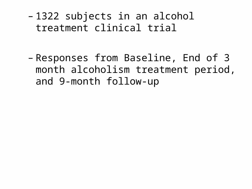
– 1322 subjects in an alcohol treatment clinical trial
– Responses from Baseline, End of 3 month alcoholism treatment period, and 9-month follow-up

• Dimensionality Assessment
Eigenvalue Ratio
Baseline 7.01 / 1.32
3-Months 7.72 / 1.23
9-Months 7.83 / 1.39

• Classical Test Theory Statistics
BaselineMean Score: 9.52 s.d. 7.94 =.90
3 MonthsMean Score: 6.75 s.d. 7.29 =.90
9 MonthsMean Score: 6.94 s.d. 7.45 =.91

• Classical Test Theory Statistics (cont.)
ITC ___ ___Time Range Obs. Obs. range
Baseline (.34, .64) .50 (.12, .76)
3 Months (.20, .72) .36 (.11, .53)
9 Months (.36, .71) .37 (.13, .53)
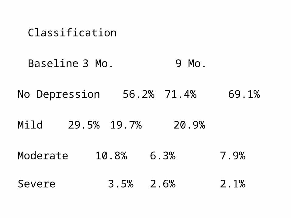
Classification
Baseline 3 Mo. 9 Mo.
No Depression 56.2% 71.4% 69.1%
Mild 29.5% 19.7% 20.9%
Moderate 10.8% 6.3% 7.9%
Severe 3.5% 2.6% 2.1%

• Parameter Estimation– Markov Chain Monte Carlo estimation with
WinBUGS
MVN(, ) prior for
N(0,4) prior for
LN(0,.25) prior for
Estimation requires two constraints on a commonitem
Set one step difficulty parameter and one discrimination parameter to constant values
1)( ti
)( ti
*
tj

• Item Parameter Estimates
Range Mean
(1.37, 2.38) 1.82
(.43, 2.73) 1.62

• Test Characteristic Curve (for Composite Theta at Time t)

• Test Information Function (for Composite Theta at Time t)

• Estimated Person Distribution Hyperparameters
Baseline .362 .861
Change from -.525 .856Baseline to TxEnd (3 Months)
Change from Tx .002 .829 End to Follow-up(3 to 9 Months)
t*ˆ j t*ˆ j

• Estimated Correlation Among Person Parameters
134.09.
34.118.
09.18.1ˆ
R
EAP Person Estimates of Latent Baseline Level and Change


Example 2: Simulated Multiple Forms Design
• Two Assessment Periods With a 20-Item Form Administered at Each Testing Period
– Four items are common across test forms
– Item parameters sampled from 3-category items from the 1998 NAEP Technical Report
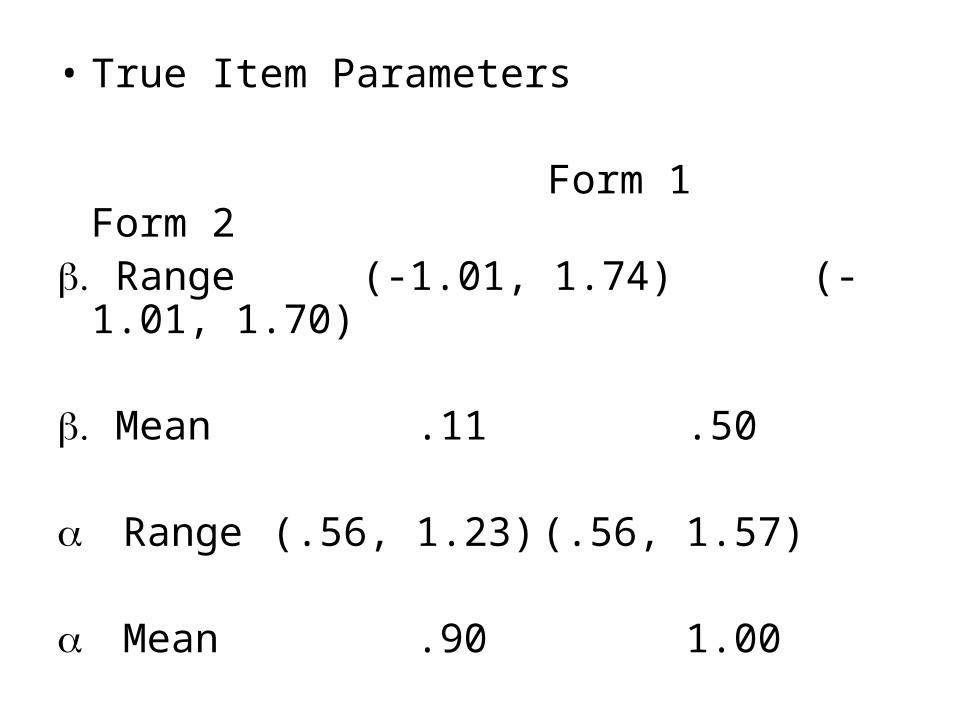
• True Item Parameters
Form 1 Form 2 Range (-1.01, 1.74) (-1.01, 1.70)
Mean .11 .50
Range (.56, 1.23) (.56, 1.57)
Mean .90 1.00

• Person Parameters at Time 1 and Change at Time 2 were Sampled From a Bivariate Normal Distribution with = -.243
j1* ~ N(0, 1)
j2* ~ N(.5, 1.0625)
• 2000 Simulees

• Estimated Item Parameters
Range MeanForm 1 Form 2 Form 1
Form 2
. ( -.99, 1.74) ( -.99, 1.87) .17 .61
(-1.01, 1.74) (-1.01, 1.70) .11 .50
(.53, 1.15) (.53, 1.43) .85 .96
(.56, 1.23) (.56, 1.57) .90 1.00
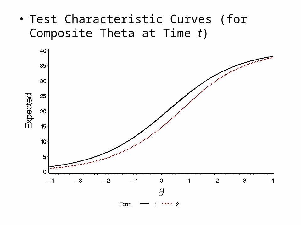
• Test Characteristic Curves (for Composite Theta at Time t)

• Test Information Functions (for Composite Theta at Time t)

• Estimated Person Distribution Hyperparameters
Time 1 .07 1.08
.00 1.00
Change from .54 1.10
Time 1 to Time 2 .50 1.03
t*ˆ j t*ˆ j

• Estimated Correlation Among Person Parameters
130.
30.1ˆR

EAP Person Estimates of Latent Baseline Level and Change


Next Steps
• Recovery Simulations– In progress, so far, so good
• Want to try this out with real student proficiency data– Do you have any to share?
• Want to investigate alternative estimation strategies for new model
– WinBUGS is really slow
– NLMIXED would probably be quite slow too
– MMAP should work well, but will require a lot of effort to develop a general program

The Sprout Model
• The assessment is p-dimensional at baseline
• Individuals change along the p dimensions, but q new dimensions “sprout” out across time
– Individuals change along the new dimensions as well

• Could look at change on all dimensions or project onto some subset of dimensions
• Similar to work that Reckase and Martineau (2004) have done with MIRT– Strategies differ in how change is parameterized– Sprout model emphasizes change over repeated
measurements of the same respondents rather than vertical scaling of cross-sectional groups
• Potential problems– Identification– Data demands required for reasonable parameter
recovery
Summary
• The multidimensional IRT approach to change has the advantages of other IRT models and can alleviate some problematic aspects to measuring change from a traditional classical test theory perspective
• The model presented here is quite general and can be applied to a variety of testing situations

• It leads to some very intuitive multi-trait generalizations
– The practicality of implementing these generalizations remains to be seen
• We are hopeful

Thanks!


![[IRT] Item Response Theory · 2019. 3. 1. · Title irt — Introduction to IRT models DescriptionRemarks and examplesReferencesAlso see Description Item response theory (IRT) is](https://img.pdfslide.us/doc/110x75/60f87abb593d3015bc4d5fae/irt-item-response-theory-2019-3-1-title-irt-a-introduction-to-irt-models.jpg)