Embed Size (px)
Citation preview
Investigation of the Gas Dispersion and Mixing
Characteristics in Column Flotation using
Computational Fluid Dynamics (CFD)
by
Ikukumbuta Mwandawande
Dissertation presented for the Degree
of
DOCTOR OF PHILOSOPHY
(Extractive Metallurgical Engineering)
in the Faculty of Engineering
at Stellenbosch University
Supervisor
Prof. G. Akdogan
Co-Supervisor
Prof. S.M. Bradshaw
March 2016

i
Declaration
By submitting this dissertation electronically, I declare that the entirety of the work contained
therein is my own, original work, that I am the sole author thereof (save to the extent
explicitly otherwise stated), that reproduction and publication thereof by Stellenbosch
University will not infringe any third party rights and that I have not previously in its entirety
or in part submitted it for obtaining any qualification.
Date: March 2016
Copyright © 2016 Stellenbosch University
All rights reserved
Stellenbosch University https://scholar.sun.ac.za

ii
Abstract
In this thesis, Computational Fluid Dynamics (CFD) was applied to study gas dispersion and
mixing characteristics of industrial and pilot scale flotation columns. An Eulerian-Eulerian
multiphase modelling approach with appropriate interphase momentum exchange terms was
applied to simulate the multiphase flow inside the column while turbulence in the continuous
phase was modelled using the k-ϵ realizable turbulence model. The CFD simulations in this
research were performed using the Ansys Fluent 14.5 CFD solver.
In the first part of the research, CFD was used to predict the average gas holdup and the axial
gas holdup variation in the collection zone of a 0.91 m diameter pilot flotation column
operated in batch mode. The axial gas holdup profile was achieved in the simulations using
the Ideal Gas law to impose compressibility effects on the air bubbles. With mean absolute
relative error (MARE) ranging from 6.2 to 10.8%, the predicted average gas holdup values
were in good agreement with experimental data. The axial gas holdup prediction was
generally good for the middle and top parts of the column where the mean absolute relative
error values were less than 10% while the gas holdup was over-predicted for the bottom part
of the column (MARE exceeding 20%), especially at lower superficial gas velocities. The
axial velocity of the air bubbles decreased with height along the column. The axial decrease
in the bubble velocity may be due to the increase in the drag force resulting from the upward
increase in gas holdup in the column. Simulations were also conducted to compare the gas
holdup predicted with three different drag models, the Universal drag coefficient, the
Schiller-Naumann, and the Morsi-Alexander drag models. The gas holdup predictions for the
three drag models were not significantly different.
Flotation columns are known for their improved metallurgical performance compared to
conventional flotation cells. However, increased mixing in the column can adversely affect its
grade/recovery performance. In the second part of this research, the mixing characteristics of
the collection zone of industrial flotation columns were investigated using CFD. Liquid and
particle residence time distribution (RTD) data were computed from CFD simulations and
subsequently used to determine the mixing parameters (the mean residence time and the
vessel dispersion number). Liquid RTD was modelled using the Species Model available in
Ansys Fluent while the particle RTD was modelled using a user defined scalar (UDS)
transport equation that computes the age of the particles in the column. The mean residence
time of particles in the column was well predicted with a mean absolute relative error equal to
Stellenbosch University https://scholar.sun.ac.za

iii
7.8%. The results obtained showed that particle residence time decreases with increasing
particle size. The residence time of the coarser particles (125 µm) was found to be about 50%
of the liquid residence time while the finer particles (44 µm) had residence time similar to the
liquid one. These findings are in agreement with experimental data available in the literature.
The relationship between the liquid and solids axial dispersion coefficients was also
investigated by comparing the water and the solids flow patterns. The flow patterns between
the phases revealed that their dispersion coefficients were similar. In addition, the effects of
the bubble size and particle size of the solids on the liquid dispersion were investigated. It
was found that increasing particle size of the solids resulted in a decrease in the liquid vessel
dispersion number. On the other hand, a decrease in the bubble size caused a significant
increase in the liquid vessel dispersion number.
Flotation columns are normally operated at optimal superficial gas velocities to maintain
bubbly flow conditions. However, with increasing superficial gas velocity, loss of bubbly
flow may occur with adverse effects on column performance. It is therefore important to
identify the maximum superficial gas velocity above which loss of bubbly flow occurs. The
maximum superficial gas velocity is usually obtained from a gas holdup versus superficial
gas velocity plot in which the linear portion of the graph represents bubbly flow while
deviation from the linear relationship indicates a change from the bubbly flow to the churn-
turbulent regime. However, this method is difficult to use when the transition from bubbly
flow to churn-turbulent flow is gradual as happens in the presence of frothers. Two
alternative methods are presented in the final part of the present research in which the flow
regime prevailing in the column is related to radial gas holdup profiles and gas holdup versus
time plots obtained from CFD simulations. The results showed that radial gas holdup profiles
can be used to distinguish bubbly flow (saddle shaped gas holdup profiles) from churn
turbulent flow (steep parabolic gas holdup profiles). However, the transitional regime
between these two extremes was difficult to characterize due to its gradual nature. Another
important finding of this research was that different radial gas holdup profiles could result in
opposite liquid flow patterns. For example, a liquid circulation pattern with upward flow in
the centre and downward flow near the column walls was always present when the radial gas
holdup profile is parabolic. On the other hand, an inverse flow pattern was observed in which
the liquid rises near the column wall but descends in the centre and adjacent to the wall. This
profile was accompanied by corresponding saddle shaped radial gas holdup profiles.
Stellenbosch University https://scholar.sun.ac.za

iv
Opsomming
In hierdie tesis word berekeningsvloeidinamika (CFD) gebruik om die gasdispersie- en
vermengingskenmerke van flottasiekolomme op industriële en proefskaal te bestudeer. ’n
Meerfasige Euler-Euler-modelleringsbenadering met toepaslike momentumuitruiling tussen
fases is gebruik om die meerfasige vloei in die kolom te simuleer. Die turbulensie in die
kontinue fase is op sy beurt met die realiseerbare k-ε-turbulensiemodel gemodelleer. Die
CFD-simulasies in hierdie navorsing is met behulp van die CFD-oplossingsagteware Ansys
Fluent 14.5 uitgevoer.
In die eerste deel van die navorsing is CFD gebruik om die gemiddelde en aksiale
gasvasvangingsvariasie te voorspel in die versamelsone van ’n proefflottasiekolom met ’n
deursnee van 0,91 m wat in lotte bedryf word. Die aksiale gasvasvangingsprofiel in die
simulasies is verkry deur van die idealegaswet gebruik te maak om ’n
saamdrukbaarheidseffek op die lugborrels uit te oefen. Met ’n gemiddelde absolute relatiewe
afwykingswaarde (MARE) van tussen 6.2 en 10.8% het die voorspelde gemiddelde
gasvasvangingswaardes sterk ooreenkomste met die eksperimentele data getoon. Die
voorspelde aksiale gasvasvangingswaardes was oor die algemeen goed vir die middelste en
boonste dele van die kolom, waar die gemiddelde absolute relatiewe afwykingswaardes
minder as 10% was. Tog was die voorspelde gasvasvangingswaardes vir die onderste
gedeelte van die kolom te hoog (met ’n MARE van meer as 20%), veral teen laer
oppervlakkige gassnelhede. Die aksiale snelheid van die lugborrels het afgeneem namate dit
hoër op in die kolom beweeg het. Dié aksiale afname in borrelsnelheid kan moontlik
toegeskryf word aan die toename in sleurkrag vanweë die verhoogde gasvasvanging hoër op
in die kolom. Daar is ook simulasies gedoen om die voorspelde gasvasvangingswaardes met
drie verskillende sleurmodelle, naamlik die universele sleurkoëffisiënt, Schiller-Naumann en
Morsi-Alexander, te vergelyk. Die voorspelde gasvasvangingswaardes vir die drie
sleurmodelle het nie beduidend verskil nie.
Flottasiekolomme is bekend vir hulle beter metallurgiese werkverrigting vergeleke met
konvensionele flottasieselle. Tog kan verhoogde vermenging in die kolom ’n negatiewe
uitwerking op graad/herwinning hê. In die tweede deel van die navorsing is die
vermengingskenmerke in die versamelsone van industriële flottasiekolomme met behulp van
CFD ondersoek. Data oor die verblyftydverspreiding (RTD) van vloeistof en deeltjies is op
grond van CFD-simulasies bereken en daarná gebruik om die vermengingsparameters
Stellenbosch University https://scholar.sun.ac.za

v
(gemiddelde verblyftyd en houerdispersiewaarde) vas te stel. Die RTD vir vloeistof is
gemodelleer met die spesiemodel in die sagteware Ansys Fluent. Die RTD vir deeltjies is op
sy beurt met ’n gebruikersomskrewe skalêre (UDS-) vervoervergelyking gemodelleer wat die
ouderdom van die deeltjies in die kolom bereken. Die gemiddelde verblyftyd van deeltjies in
die kolom is akkuraat voorspel, met ’n gemiddelde absolute relatiewe afwykingswaarde van
7.8%. Die resultate toon dat deeltjieverblyftyd afneem namate deeltjiegrootte toeneem. Die
verblyftyd van die growwer deeltjies (125 µm) blyk sowat 50% van die vloeistofverblyftyd te
wees, terwyl die verblyftyd van die fyner deeltjies (44 µm) soortgelyk is aan dié van
vloeistof. Hierdie bevindinge stem ooreen met die eksperimentele data wat in die literatuur
beskikbaar is. Die verwantskap tussen die aksiale dispersiekoëffisiënte vir vloeistof en vaste
stowwe is ook ondersoek deur die vloeipatrone van water en vaste stowwe te vergelyk. Die
vloeipatrone tussen die fases dui op soortgelyke dispersiekoëffisiënte. Daarbenewens is die
uitwerking van die borrelgrootte en deeltjiegrootte van vaste stowwe op vloeistofdispersie
ondersoek. Daar is bevind dat ’n toename in die deeltjiegrootte van vaste stowwe ’n afname
in die houerdispersiewaarde van vloeistof tot gevolg het. Daarteenoor lei ’n afname in
borrelgrootte tot ’n beduidende toename in die houerdispersiewaarde van vloeistof.
Flottasiekolomme word gewoonlik teen optimale oppervlakkige gassnelhede bedryf om
borrelvloei-omstandighede te handhaaf. Namate oppervlakkige gassnelheid egter toeneem,
kan borrelvloei afneem, wat ’n nadelige uitwerking op die werkverrigting van die kolom kan
hê. Daarom is dit belangrik om die maksimum oppervlakkige gassnelheid te bepaal waarbo
borrelvloei afneem. Hierdie maksimum oppervlakkige gassnelheid word gewoonlik verkry
deur middel van ’n grafiek van gasvasvanging teenoor oppervlakkige gassnelheid, waar die
lineêre gedeelte van die grafiek die borrelvloei voorstel, en afwyking van die lineêre
verwantskap op ’n verandering van die borrelvloei- na die kolk-turbulente vloeiregime dui.
Tog is dit moeilik om hierdie metode te gebruik as die oorgang van borrel- na kolk-turbulente
vloei geleidelik plaasvind, soos wanneer daar skuimmiddels betrokke is. In die laaste deel
van die navorsing word twee alternatiewe metodes aangebied waarin die heersende
vloeiregime in die kolom vergelyk word met die radiale gasvasvangingsprofiele en die
gasvasvanging/tyd-grafieke wat uit die CFD-simulasies verkry is. Die resultate toon dat
radiale gasvasvangingsprofiele gebruik kan word om borrelvloei (saalvormige
gasvasvangingsprofiele) van kolk-turbulente vloei (steil paraboliese gasvasvangingsprofiele)
te onderskei. Die oorgangsregime tussen hierdie twee uiterstes was egter moeilik om te tipeer
weens die geleidelike aard daarvan. ’n Verdere belangrike bevinding van hierdie navorsing is
Stellenbosch University https://scholar.sun.ac.za
vi
dat verskillende radiale gasvasvangingsprofiele tot teenoorgestelde vloeistofvloeipatrone kan
lei. ’n Vloeistofsirkulasiepatroon met opwaartse vloei in die middel en afwaartse vloei naby
die kolomwande was byvoorbeeld deurentyd teenwoordig toe die radiale
gasvasvangingsprofiel parabolies was. Daarteenoor is ’n omgekeerde vloeipatroon
waargeneem waarin die vloeistof naby die kolomwand styg, maar in die middel en langs die
wand daal, welke profiel met saalvormige radiale gasvasvangingsprofiele gepaardgegaan het.
Stellenbosch University https://scholar.sun.ac.za

vii
Acknowledgements
I would like to acknowledge several people who have provided support or advice during the
course of my PhD research. First and foremost I would like to acknowledge the Centre for
International Cooperation at VU University Amsterdam (CIS-VU) and the Copperbelt
University (CBU) for offering me a PhD scholarship through the Nuffic-HEART Project. I
would also like to convey my sincere gratitude to my supervisors Professor Guven Akdogan
and Professor Steven Bradshaw for their valuable advice and encouragement throughout my
research programme.
I would also like to thank my colleagues and fellow research students, Mohsen, Deside,
Bawemi, Arthur, Henri, Clyde and Edson for the advice and friendships during my research
journey.
My gratitude also goes to Stephan Schmitt and Dawie Marais at Qfinsoft for their willingness
to provide advice regarding the ANSYS FLUENT software.
Finally, let me thank my wife Lenny and my son Michael for their valued support, love,
understanding and patience.
Stellenbosch University https://scholar.sun.ac.za

viii
Dedication
This thesis is dedicated to the late Professor Glasswell Nkonde for supporting me to come
and study at Stellenbosch University. May His Soul Rest In Peace.
Stellenbosch University https://scholar.sun.ac.za

ix
Table of Contents
Declaration .................................................................................................................................. i
Abstract ...................................................................................................................................... ii
Opsomming ............................................................................................................................... iv
Acknowledgements .................................................................................................................. vii
Dedication .............................................................................................................................. viii
Table of Contents ...................................................................................................................... ix
List of Figures .......................................................................................................................... xv
List of Tables .......................................................................................................................... xix
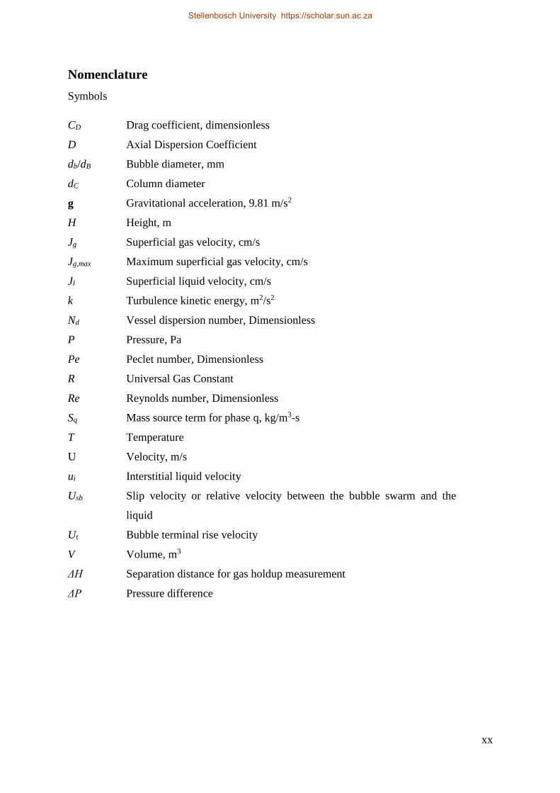
Nomenclature ........................................................................................................................... xx
Chapter 1 Introduction .......................................................................................................... 1
1.1 Background ................................................................................................................ 1
1.2 Objectives .................................................................................................................. 4
1.3 Scope and Limitations................................................................................................ 4
1.4 Scientific contributions and Novelty ......................................................................... 7
1.5 Thesis Structure ......................................................................................................... 8
Chapter 2 Literature Review............................................................................................... 10
2.1 Introduction .............................................................................................................. 10
2.2 Gas dispersion .......................................................................................................... 10
2.2.1 Superficial gas velocity and its effects on flotation column performance ......... 10
2.2.1.1 Maximum superficial gas velocity in column flotation .............................. 10
2.2.2 Gas Holdup ........................................................................................................ 12
2.2.2.1 Gas holdup measurement techniques ......................................................... 13
2.2.2.2 Axial gas holdup distribution ..................................................................... 14
2.2.2.3 Radial gas holdup distribution .................................................................... 14
2.2.2.4 Liquid Circulation in the Column ............................................................... 15
2.2.3 Bubble Size ........................................................................................................ 15
Stellenbosch University https://scholar.sun.ac.za

x
2.2.4 Bubble surface area flux (Sb) ............................................................................. 16
2.3 Mixing ...................................................................................................................... 17
2.4 CFD models of column flotation in the literature .................................................... 21
2.5 Conclusion ............................................................................................................... 28
Chapter 3 Simulation Methodology ................................................................................... 30
3.1 Introduction .............................................................................................................. 30
3.2 Model geometry, mesh and boundary conditions .................................................... 30
3.2.1 Defining the computational domain................................................................... 30
3.2.2 Modelling of the spargers .................................................................................. 31
3.2.2.1 Calculation of mass and momentum source terms ..................................... 31
3.2.3 Boundary conditions .......................................................................................... 32
3.2.3.1 Batch operated columns .............................................................................. 32
3.2.3.2 Continuously operated columns ................................................................. 32
3.2.4 Mesh size and grid independence considerations .............................................. 32
3.3 Multiphase model..................................................................................................... 32
3.3.1 Overview of multiphase models ........................................................................ 32
3.3.2 Choice of multiphase model for the present research ........................................ 33
3.3.3 Eulerian-Eulerian multiphase model.................................................................. 34
3.4 Turbulence model .................................................................................................... 35
3.4.1 Overview of turbulence modelling methods ...................................................... 35
3.4.2 Choice of turbulence model for the present research ......................................... 37
3.4.3 Realizable k-ϵ turbulence model ........................................................................ 38
3.4.4 Turbulence near the column wall ....................................................................... 39
3.5 Numerical simulation set up and solution methods ................................................. 41
Chapter 4 Numerical prediction of gas holdup and its axial variation in a flotation column
44
4.1 Introduction .............................................................................................................. 44
Stellenbosch University https://scholar.sun.ac.za

xi
4.2 Description of the column ........................................................................................ 45
4.3 CFD Model description............................................................................................ 47
4.3.1 Model geometry and mesh ................................................................................. 47
4.3.2 Boundary conditions .......................................................................................... 50
4.3.3 Multiphase Model .............................................................................................. 50
4.3.3.1 Drag force formulations .............................................................................. 51
4.3.4 Turbulence model .............................................................................................. 54
4.3.5 Numerical solution methods .............................................................................. 54
4.4 Results and discussion ............................................................................................. 55
4.4.1 Simulation results with Universal drag coefficient ............................................ 55
4.4.1.1 Liquid flow field ......................................................................................... 55
4.4.1.2 Gas holdup distribution in the column ....................................................... 57
4.4.1.3 Comparison of predicted gas holdup with experimental data .................... 59
4.4.1.4 Bubble velocities ........................................................................................ 62
4.4.2 Comparison of average and axial gas holdup predicted using different drag
coefficients ........................................................................................................................ 65
4.5 Conclusions .............................................................................................................. 74
Chapter 5 CFD Simulation of the mixing characteristics of industrial flotation columns . 75
5.1 Introduction .............................................................................................................. 75
5.2 Theory ...................................................................................................................... 77
5.3 CFD Methodology ................................................................................................... 78
5.3.1 Model geometry, mesh, and boundary conditions ............................................. 78
5.3.1.1 Grid independence study (0.45 m square column) ..................................... 80
5.3.1.2 Grid independency study (0.91 m diameter cylindrical column) ............... 82
5.3.2 Multiphase model............................................................................................... 84
5.3.2.1 Gas-liquid drag force .................................................................................. 85
5.3.2.2 Liquid-solid drag force ............................................................................... 86
Stellenbosch University https://scholar.sun.ac.za
xii
5.3.3 Turbulence model .............................................................................................. 86
5.3.4 Residence Time Distribution (RTD) Simulation ............................................... 87
5.3.4.1 Liquid RTD................................................................................................. 87
5.3.4.2 Particle (Solids) RTD ................................................................................. 89
5.4 Results and discussion ............................................................................................. 90
5.4.1 Square column ................................................................................................... 91
5.4.1.1 Liquid residence time distribution (RTD) .................................................. 91
5.4.1.2 Particle (solids) RTD .................................................................................. 92
5.4.1.3 Comparison of liquid (water) and solids flow patterns .............................. 95
5.4.2 Cylindrical column............................................................................................. 97
5.4.2.1 Liquid residence time distribution (RTD) .................................................. 97
5.4.2.2 Particle (solids) RTD ................................................................................ 101
5.4.2.3 Comparison of liquid and solids flow patterns at higher solids content (16.2
wt% solids).................................................................................................................. 102
5.5 Conclusion ............................................................................................................. 104
Chapter 6 Investigation of flow regime transition in a column flotation cell using CFD 106
6.1 Introduction ............................................................................................................ 106
6.2 Methods for flow regime identification ................................................................. 107
6.2.1 Radial Gas Holdup profiles .............................................................................. 108
6.2.2 Gas holdup versus Time graph ........................................................................ 109
6.3 Description of the modeled column ....................................................................... 109
6.4 CFD Methodology ................................................................................................. 110
6.4.1 Geometry and mesh ......................................................................................... 110
6.4.2 Boundary conditions ........................................................................................ 113
6.4.3 Multiphase Model ............................................................................................ 113
6.4.4 Turbulence Modeling ....................................................................................... 114
6.4.5 Numerical solution methods ............................................................................ 115
Stellenbosch University https://scholar.sun.ac.za
xiii
6.5 Results and discussion ........................................................................................... 115
6.5.1 Water and air only (without frother) ................................................................ 116
6.5.1.1 Gas holdup versus superficial gas velocity (gas rate) graph .................... 117
6.5.1.2 Radial gas holdup profiles ........................................................................ 118
6.5.1.3 Gas holdup versus time graphs ................................................................. 120
6.5.2 Water with frother (as in column flotation) ..................................................... 125
6.5.3 Maximum superficial gas velocity for a column operating with 1.5 mm average
bubble size ...................................................................................................................... 126
6.5.4 Liquid Velocity vectors.................................................................................... 131
6.5.5 Effect of interphase turbulent dispersion on radial gas holdup profile ............ 134
6.5.6 Applicability of radial gas holdup profiles for flow regime characterization in
large diameter columns ................................................................................................... 135
6.6 Conclusions ............................................................................................................ 136
Chapter 7 Conclusions and Recommendations ................................................................ 138
7.1 Research summary ................................................................................................. 138
7.2 Conclusions ............................................................................................................ 140
7.2.1 Gas holdup and its distribution in the column ................................................. 140
7.2.2 Mixing characteristics of the collection zone in column flotation ................... 140
7.2.3 Flow regime identification using CFD ............................................................ 141
7.3 Recommendations .................................................................................................. 142
References .............................................................................................................................. 143
Appendix 1: Mass and momentum source terms for the simulations in Chapter 4 . ............. 157
Appendix 2: User defined function for the source term used in particle age transport equation
................................................................................................................................................ 158
Appendix 3: Mass and momentum source terms for the simulations in Chapter 6. .............. 159
Appendix 4: Drag coefficient calculations used for the CD versus Re graphs in Figure 4.6. 160
Appendix 5: Predicted turbulence quanties at mid-height position for the column (0.91 m
diameter) simulated in Chapter 4. .......................................................................................... 163
Stellenbosch University https://scholar.sun.ac.za

xiv
Appendix 6: Some turbulence quantities taken at mid-height position for the column
simulated in Chapter 6 for bubbly flow and churn-turbulent flow conditions. ..................... 165
Stellenbosch University https://scholar.sun.ac.za

xv
List of Figures
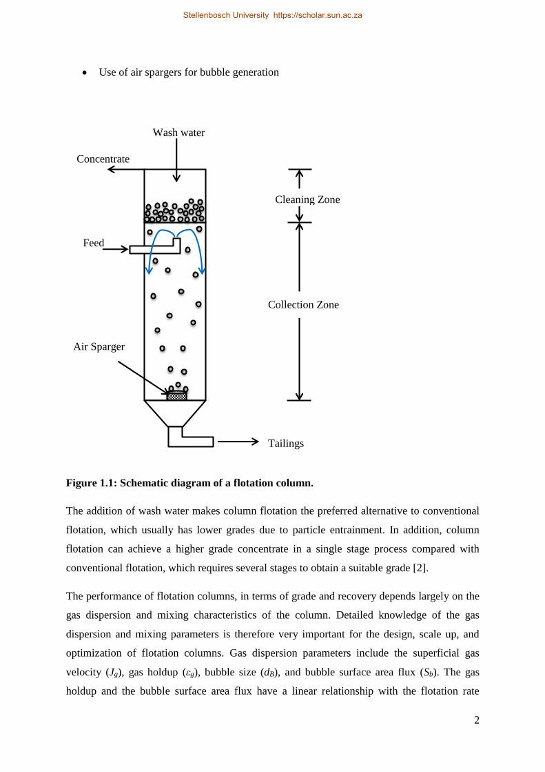
Figure 1.1: Schematic diagram of a flotation column................................................................ 2
Figure 2.1: Methods of measuring gas holdup (adapted from Finch and Dobby [2]). ............ 13
Figure 2.2: Recovery as a function of the dimensionless product kτ for different values of Nd
(Redrawn from Luttrell et al. [56]). ......................................................................................... 18
Figure 3.1: Comparison of the two approaches that can be used for near wall treatment in
CFD simulations (Adapted from Bengt et al. [72]). ................................................................ 41
Figure 3.2: The SIMPLE algorithm (adapted from Versteeg and Malalasekera [71]). ........... 43
Figure 4.1: position of pressure sensing devices and their distance from the top of the column
(adapted from Gomez et al. [18]). ............................................................................................ 46
Figure 4.2: CFD model geometry of the experimental pilot column. ...................................... 47
Figure 4.3: CFD mesh for the 0.91 m diameter cylindrical column. ....................................... 48
Figure 4.4: Simulated axial water velocity profiles for the investigated mesh sizes
(Superficial gas velocity, Jg = 1.51 cm/s). ............................................................................... 49
Figure 4.5: Simulated bubble velocity profiles for the different mesh sizes (Superficial gas
velocity, Jg = 1.51 cm/s). ......................................................................................................... 50
Figure 4.6: Drag coefficient CD as a function of bubble Reynolds number Re for 0 ≤ Re <
1000.......................................................................................................................................... 54
Figure 4.7: Vectors showing the predicted flow of water in the column (superficial gas
velocity, Jg = 0.93 cm/s). ......................................................................................................... 56
Figure 4.8: Axial water velocity profile at column mid-height position (Height = 6.75 m).
Superficial gas velocity, Jg = 0.93 cm/s. .................................................................................. 57
Figure 4.9: Gas holdup contours – time averaged air volume fraction (Jg = 0.93 cm/s). ........ 58
Figure 4.10: Comparison of CFD simulations with hydrostatic pressure effects
(compressibility) and the case without hydrostatic bubble 'expansion' (incompressible); Jg =
1.51 cm/s. ................................................................................................................................. 59
Figure 4.11: Parity plot comparing the predicted (CFD) average gas holdup and the
experimental data [18]. ............................................................................................................ 60
Figure 4.12: Comparison of the predicted axial gas holdup profile with experimental data
[18]; Jg = 0.72 cm/s. ................................................................................................................. 61
Figure 4.13: Comparison of the predicted axial gas holdup profile with experimental data
[18]; Jg = 0.93 cm/s. ................................................................................................................. 61
Stellenbosch University https://scholar.sun.ac.za
xvi
Figure 4.14: Comparison of the predicted axial gas holdup profile with experimental data
[18]; Jg = 1.51 cm/s. ................................................................................................................. 62
Figure 4.15: Comparison of the predicted axial gas holdup profile with experimental data
[18]; Jg = 1.67 cm/s. ................................................................................................................. 62
Figure 4.16: Axial velocity profiles of air bubbles at three different heights along the column;
Jg = 1.51 cm/s. .......................................................................................................................... 64
Figure 4.17: Axial bubble velocity versus height along the column axis; Jg = 1.51 cm/s. ...... 65
Figure 4.18: Parity plot comparing the average gas holdup prediction for different drag
models. The different models are compared against the experimental data from Gomez et
al.[18] ....................................................................................................................................... 66
Figure 4.19: Comparison of axial gas holdup prediction for different drag coefficients;
superficial gas velocity, Jg = 0.72 cm/s. .................................................................................. 68
Figure 4.20: Comparison of axial gas holdup prediction for different drag coefficients;
superficial gas velocity, Jg = 0.93 cm/s. .................................................................................. 69
Figure 4.21: Comparison of gas holdup prediction for different drag coefficients; superficial
gas velocity, Jg = 1.51 cm/s. .................................................................................................... 69
Figure 4.22: Comparison of gas holdup prediction for different drag coefficients; superficial
gas velocity, Jg = 1.67 cm/s. .................................................................................................... 70
Figure 5.1: Computational mesh for the 0.45 m square column (side view). .......................... 79
Figure 5.2: Computational mesh for the 0.91 m diameter cylindrical column. ....................... 80
Figure 5.3: Simulated mean axial bubble velocities for different mesh sizes (0.45 m square
column). ................................................................................................................................... 81
Figure 5.4: Simulated mean axial liquid (water) velocities for different mesh sizes (0.45 m
square column). ........................................................................................................................ 82
Figure 5.5: Simulated mean axial bubble velocity profiles for the different mesh sizes (0.91 m
diameter column). .................................................................................................................... 83
Figure 5.6: Simulated mean axial liquid velocity profiles for the different mesh sizes (0.91 m
diameter column). .................................................................................................................... 84
Figure 5.7: Simulated liquid (water) RTD for the square column compared with the
experimental data of Dobby and Finch [58]. ........................................................................... 92
Figure 5.8: Contours of simulated particle age distribution in the square column; particle size
= 44 µm. ................................................................................................................................... 93
Figure 5.9: Axial velocity profile of water showing the circulation pattern with upward flow
at the centre and downward flow near the column walls (square column). ............................. 94
Stellenbosch University https://scholar.sun.ac.za

xvii
Figure 5.10: Comparison of CFD predicted (simulation) and experimental measurements [58]
of particle mean residence time vs particle size. ...................................................................... 95
Figure 5.11: Comparison of liquid (water) and solids (88 µm) axial velocity profiles. .......... 96
Figure 5.12: Comparison of liquid (water) and solids (125 µm) axial velocity profiles. ........ 97
Figure 5.13: Simulated liquid (water) RTD for the cylindrical column compared with the
experimental data of Yianatos and Bergh [65]. ....................................................................... 98
Figure 5.14: Effect of particle size on the liquid vessel dispersion number. The results are
from CFD simulations performed with two different bubble sizes, namely 0.8 and 1 mm
(cylindrical column). .............................................................................................................. 100
Figure 5.15: Effect of bubble size on the liquid vessel dispersion number (cylindrical
column). ................................................................................................................................. 100
Figure 5.16: Spatial distribution of particle age for 112.5 µm particles; bubble size = 1 mm.
................................................................................................................................................ 101
Figure 5.17: Comparison of water velocity vectors with particle age contours in the column.
................................................................................................................................................ 102
Figure 5.18: Comparison of liquid (water) and solids (56.5 µm) axial velocity profiles. ..... 103
Figure 5.19: Comparison of liquid (water) and solids (112.5 µm) axial velocity profiles. ... 104
Figure 6.1: Gas holdup as a function of superficial gas velocity (adapted from Finch and
Dobby[2]). .............................................................................................................................. 108
Figure 6.2: Schematic diagram of the modelled experimental column (after Xu et al. [20].).
................................................................................................................................................ 110
Figure 6.3: Water velocity profiles at mid-height in the collection zone (Height = 152.5 cm).
................................................................................................................................................ 112
Figure 6.4: Bubble velocity profiles at mid-height in the collection zone (Height = 152.5 cm).
................................................................................................................................................ 112
Figure 6.5: CFD predicted gas holdup as a function of superficial gas velocity. .................. 118
Figure 6.6: Radial gas holdup profile at Jg = 1.84 cm/s in the bubbly flow regime. The profile
is saddle shaped with three distinct peaks.............................................................................. 119
Figure 6.7: Radial gas holdup profiles at Jg = 4.44 cm/s in the bubbly flow regime. The
saddle shaped profile is characterised by two near wall peaks and a central minimum value.
................................................................................................................................................ 119
Figure 6.8: Radial gas holdup profile at Jg = 6.12 cm/s (Jgmax) showing a flat profile with
features intermediate between saddle and parabolic profiles. ............................................... 120
Stellenbosch University https://scholar.sun.ac.za
xviii
Figure 6.9: Radial gas holdup profile at Jg = 14 cm/s in the churn-turbulent flow regime. The
typical profile is a steep parabolic profile. ............................................................................. 121
Figure 6.10: Gas holdup versus time graph for Jg = 1.84 cm/s. The constant gas holdup
indicates bubbly flow conditions in the column. ................................................................... 121
Figure 6.11: Gas holdup versus time graph for Jg = 14 cm/s. The wide variations in gas
holdup are a characteristic feature of the churn-turbulent flow regime. ................................ 122
Figure 6.12: Comparison of CFD predicted gas holdup with experimental data [19]. .......... 126
Figure 6.13: Radial gas holdup profile at Jg = 1.01 cm/s (Bubble size = 1.5 mm). ............... 127
Figure 6.14: Gas holdup versus Time for Jg = 1.01 cm/s (Bubble size = 1.5 mm). .............. 127
Figure 6.15: Radial gas holdup profile at Jg,max (3.12 cm/s). ................................................. 128
Figure 6.16: Gas holdup versus Time graph for Jg = 3.12 cm/s (Jg,max); bubble size = 1.5 mm.
................................................................................................................................................ 129
Figure 6.17: Radial gas holdup profile at Jg = 5.28 cm/s (bubble size = 1.5 mm). ............... 130
Figure 6.18: Gas holdup versus Time graph for Jg = 5.28 cm/s (bubble size = 1.5 mm). ..... 130
Figure 6.19: Liquid velocity vectors at mid-height in the collection zone for Jg = 4.03 cm/s
(Gulf-stream circulation pattern). .......................................................................................... 133
Figure 6.20: Liquid velocity vectors at mid-height in the collection zone for Jg = 1.54 cm/s
(Inverse circulation pattern). .................................................................................................. 134
Figure 6.21: Effect of turbulent dispersion on the simulated radial gas holdup profile. ....... 135
Stellenbosch University https://scholar.sun.ac.za
xix
List of Tables
Table 2.1: Previous literature on CFD modelling of column flotation. ................................... 27
Table 3.1: RANS based turbulence models. ............................................................................ 37
Table 3.2: Turbulence model constants. .................................................................................. 39
Table 4.1: Mesh sizes investigated in the grid dependence study. .......................................... 49
Table 4.2: The drag coefficients that were used in the CFD simulations in the present study.
.................................................................................................................................................. 53
Table 4.3: Parameters used in the CFD simulations. ............................................................... 55
Table 4.4: Predicted average velocities of air bubbles at different superficial gas velocities. 63
Table 4.5: Comparison of average gas holdup predicted using different drag coefficients. ... 67
Table 4.6: Comparison of axial gas holdup predicted with different drag coefficients for the
bottom section of the column. The drag coefficients are compared against the experimental
data of Gomez et al.[18]........................................................................................................... 71
Table 4.7: Comparison of axial gas holdup predicted with different drag coefficients for the
middle section of the column. The drag coefficients are compared against the experimental
data of Gomez et al.[18]........................................................................................................... 72
Table 4.8: Comparison of axial gas holdup predicted with different drag coefficients for the
top section of the column. The drag coefficients are compared against the experimental data
of Gomez et al.[18]. ................................................................................................................. 73
Table 5.1: Mesh sizes considered for the grid independency study (0.45 m square column). 81
Table 5.2: Mesh sizes considred for the grid independency study (0.91 m diameter column).
.................................................................................................................................................. 82
Table 5.3: Operating conditions of the industrial columns being simulated in the present study
[58, 65]. .................................................................................................................................... 90
Table 5.4: Comparison of CFD predicted mixing parameters with experimental data. .......... 92
Table 5.5: Comparison of CFD predicted (simulated) mixing parameters with experimental
data. .......................................................................................................................................... 98
Table 6.1: The five mesh sizes and their respective characteristics. ..................................... 111
Table 6.2: Summary of CFD simulation of the water and air system (without frother); Jg,max =
6.12 cm/s. ............................................................................................................................... 123
Table 6.3: Summary of the characteristics of the different flow regimes. ............................. 124
Table 6.4: Summary of CFD simulation results for 1.5 mm bubble size. ............................. 131
Stellenbosch University https://scholar.sun.ac.za
xx
Nomenclature
Symbols
CD Drag coefficient, dimensionless
D Axial Dispersion Coefficient
db/dB Bubble diameter, mm
dC Column diameter
g Gravitational acceleration, 9.81 m/s2
H Height, m
Jg Superficial gas velocity, cm/s
Jg,max Maximum superficial gas velocity, cm/s
Jl Superficial liquid velocity, cm/s
k Turbulence kinetic energy, m2/s2
Nd Vessel dispersion number, Dimensionless
P Pressure, Pa
Pe Peclet number, Dimensionless
R Universal Gas Constant
Re Reynolds number, Dimensionless
Sq Mass source term for phase q, kg/m3-s
T Temperature
U Velocity, m/s
ui Interstitial liquid velocity
Usb Slip velocity or relative velocity between the bubble swarm and the
liquid
Ut Bubble terminal rise velocity
V Volume, m3
ΔH Separation distance for gas holdup measurement
ΔP Pressure difference
Stellenbosch University https://scholar.sun.ac.za

xxi
Greek letters
𝜎𝑘 Turbulent Prandtl number for turbulence kinetic energy, k
ε Phase volume fraction (holdup)
ϵ Turbulence dissipation rate, m2/s3
εg Gas holdup
μ Viscosity, kg/m-s
μt Turbulent viscosity, kg/m-s
ρ Density, kg/m3
ρsl Slurry density
σ2 Variance
σϵ Turbulent Prandtl number for turbulence dissipation rate, ϵ
σϴ2 Relative variance
τ Mean residence time
𝜏𝑞̿̿ ̿ Stress-strain tensor
Subscripts
B Bubble
D Drag
G, g Gas
i, j Spatial directions
L, l Liquid
q Phase
Abbreviations
ADM Axial Dispersion Model
CFD Computational Fluid Dynamics
DNS Direct Numerical Simulation
DPM Discrete Phase Model
LES Large Eddy Simulation
LSTS Large and Small Tanks in Series
MAC Marker and Cell
MARE Mean Absolute Relative Error
Stellenbosch University https://scholar.sun.ac.za
xxii
PDE Partial Differential Equation
QUICK Quadratic Upstream Interpolation for Convective Kinetics
RANS Reynolds-Averaged Navier Stokes
RTD Residence Time Distribution
SIMPLE Semi-Implicit Method for Pressure-Linked Equations
TSTE Taylor Series Truncation Error
UDF User Defined Function
UDS User Defined Scalar
VOF Volume of Fluid
Stellenbosch University https://scholar.sun.ac.za
1
Chapter 1 Introduction
1.1 Background
Column flotation was invented in 1962 [1]. However, the first commercial size unit, a 36 inch
diameter column was unsuccessful due to mechanical problems. It was only after several
years that another unit, an 18 inch square column, was built in order to carry out tests and
modifications to subsequently improve the larger column. The development work on the 18
inch column was successfully completed in 1967 and an identical 18 inch column was later
installed in the first commercial operation at Mines Gaspé (in Quebec, Canada) in 1980 for
Mo cleaning. The flotation column proved to perform better than conventional flotation cells,
with a single column stage replacing several stages of conventional cells [2].
Over the years, column flotation has become a very important concentration technology used
in mineral processing and coal beneficiation industries. However, flotation columns have also
found other applications outside mineral processing such as de-inking of recycled paper [3].
The concentration process in column flotation is achieved through the collection of the
valuable hydrophobic mineral particles by a rising swarm of air bubbles in counter-current
flow against a slurry feed. The bubbles, which are formed by bubble generators (spargers)
located near the column bottom then transport the mineral particles to the froth zone where
the particles are eventually recovered in the overflow. Wash water is added continuously at
the top of the column in order to maintain a net downward flow of water that eliminates
entrained unwanted particles and stabilizes the froth. This net downward flow of water is
referred to as positive bias flow [2]. A schematic diagram of the flotation column is presented
in Figure 1.1.
The column volume is divisible into two sections: the collection zone in which bubbles
collect the floatable mineral particles, and the cleaning zone (or froth zone) where wash water
removes the unwanted particles entrained in the water crossing with bubbles from the
collection zone. The two zones are separated by an interface which defines the froth depth or
the interface level. Column flotation differs from conventional flotation in three major
aspects:
Addition of wash water to eliminate entrainment
Absence of mechanical agitation
Stellenbosch University https://scholar.sun.ac.za
2
Use of air spargers for bubble generation
Figure 1.1: Schematic diagram of a flotation column.
The addition of wash water makes column flotation the preferred alternative to conventional
flotation, which usually has lower grades due to particle entrainment. In addition, column
flotation can achieve a higher grade concentrate in a single stage process compared with
conventional flotation, which requires several stages to obtain a suitable grade [2].
The performance of flotation columns, in terms of grade and recovery depends largely on the
gas dispersion and mixing characteristics of the column. Detailed knowledge of the gas
dispersion and mixing parameters is therefore very important for the design, scale up, and
optimization of flotation columns. Gas dispersion parameters include the superficial gas
velocity (Jg), gas holdup (εg), bubble size (dB), and bubble surface area flux (Sb). The gas
holdup and the bubble surface area flux have a linear relationship with the flotation rate
Cleaning Zone
Collection Zone
Feed
Tailings
Air Sparger
Concentrate
Wash water
Stellenbosch University https://scholar.sun.ac.za
3
constant [4] suggesting that these two parameters affect flotation column performance. The
bubble surface area flux has been recognised as the key factor that can be used to characterise
flotation machines. However, some researchers have found a linear relationship between the
gas holdup and the bubble surface area flux [5, 6]. The gas holdup was therefore suggested to
be used in place of the bubble surface area flux to characterise the flotation process. This
could be advantageous since gas holdup is easier to measure.
On the other hand, the bubble surface area flux and the gas holdup are both determined by the
superficial gas velocity and the bubble size. The superficial gas velocity also determines the
prevailing flow regime in the column. There are two types of flow conditions that can occur
in a flotation column, the bubbly flow regime characterized by uniform flow of bubbles of
uniform size, and the churn-turbulent flow regime characterized by large bubbles rising
rapidly in the collection zone causing liquid circulation. The bubbly flow regime is the
optimal condition for flotation column operation [2, 7, 8]. However, excessive superficial gas
velocity may cause loss of bubbly flow and subsequently cause a reduction in column
performance. Excessive superficial gas velocity may also result in loss of the collection
zone/cleaning zone interface, resulting in poor concentrate grade.
Mixing of the various phases in the flotation column has also emerged as one of the important
factors which affect both the particle-bubble attachment and detachment processes [9, 10]. A
high degree of mixing will therefore have a detrimental effect on the overall performance of a
flotation column. The mixing parameters which are used to characterise axial mixing in the
collection zone include the vessel dispersion number and the mean residence time of the
liquid and solid phases. Mixing parameters are used to quantify the effect of mixing upon
recovery [2].
Because of their significance in column flotation, gas dispersion and mixing parameters have
been the focus of a large number of research publications in the mineral processing field. On
the other hand, Computational Fluid Dynamics (CFD) has emerged as a numerical modelling
tool that can be used to increase the understanding of the complex hydrodynamics pertaining
to flotation cells [11-14]. However, there are a limited number of research publications on
CFD modelling of column flotation. The earliest CFD model of column flotation was a two-
dimensional two-phase fluid dynamic model presented by Deng et al. [11]. The model was
used to simulate liquid and gas flow patterns in the column using the MAC (Marker and Cell)
Stellenbosch University https://scholar.sun.ac.za
4
numerical method. Subsequent CFD based models of column flotation have been published
focusing on different aspects of the process [13-17].
In general, the existing CFD research on column flotation seems to have adequately
addressed bubble-particle interaction processes such as collision efficiencies, attachment, and
detachment [13, 16]. On the other hand, the gas dispersion and mixing parameters have not
been adequately studied. The aim of the present research was therefore to apply CFD
methodology to investigate the gas dispersion and mixing parameters in industrial and pilot
scale flotation columns.
1.2 Objectives
The main objective of this research was to apply CFD modelling to investigate the gas
dispersion and mixing parameters as well as their relationship to flotation column
performance. In order to accomplish this main objective the research was divided into smaller
objectives as outlined below:
To formulate a CFD model capable of predicting gas dispersion and mixing in the
flotation column
To carry out CFD simulations to determine the following gas dispersion parameters
o Gas holdup and its distribution in the column
o Maximum superficial gas velocity for flotation column operation
To perform CFD simulations of mixing in the column in order to determine the
following parameters
o The liquid residence time distribution RTD
o The liquid mean residence time
o The vessel dispersion number for the liquid phase
o The Particle mean residence time
To investigate the effects of gas dispersion parameters on the liquid flow patterns and
mixing conditions in in the column
To validate the CFD results with experimental data that is available in the literature
1.3 Scope and Limitations
The focus of this research is on the hydrodynamics and mixing characteristics of the
collection zone in flotation columns. In the hydrodynamics part of the research, CFD
Stellenbosch University https://scholar.sun.ac.za
5
modelling is applied to predict both the average and local gas holdup, and bubble velocities in
the collection zone of the column. CFD simulations are also used to investigate regime
transition from bubbly flow to churn-turbulent flow in order to determine the maximum
superficial gas velocity for column flotation.
The experimental work of Gomez et al. [18] is used in the present research for validation of
the gas holdup predictions while the maximum superficial gas velocity predictions are
compared against different experimental and theoretical results available in the literature [19-
21]. Since the corresponding experimental research was performed in two-phase systems with
water and air only (in the presence of frother), two-phase simulations are conducted in the
hydrodynamics part of the present study in order to simulate the actual conditions that were
used in the experiments.
On the other hand, the second part of the present research involves three-phase CFD
simulations which are conducted in order to investigate liquid and solids mixing in industrial
flotation columns. The actual flotation process in terms of bubble-particle collisions,
attachment, and detachment is beyond the scope of the present research. However, these
aspects have already been adequately studied by previous researchers notably Nadeem et al.
[16] and Kho and Schwarz [13]. The present work therefore simulates the multiphase flow
occurring in column flotation without incorporating bubble-particle interactions. The mixing
parameters in flotation columns are mostly determined by the gas holdup (i.e., gas rate and
bubble size) and the superficial liquid velocities. However, the presence of solids in bubble
columns has been reported to have an influence on gas holdup due to its effects on bubble
coalescence [22]. The predicted gas holdup in the CFD simulations is therefore limited to the
influence from the superficial gas velocity, superficial liquid velocity, and bubble size used in
the simulations.
The collection zone and the cleaning zone of a flotation column are known to have different
hydrodynamic characteristics. Although it would be desirable to formulate a CFD model that
includes both zones, the differences in turbulence and flow behaviour and the complex mass
transfer occurring at the interface will make it difficult to obtain a single simulation that
combines the two zones [23]. The CFD models applied in the present research therefore
consider the collection zone of the columns while the froth zone is not modelled. Similarly,
Deng et al. [11] did not include the froth zone in their CFD model. For column scale up
purposes, previous researchers have suggested that the recovery in the distinct zones can be
Stellenbosch University https://scholar.sun.ac.za
6
modelled independently and then combined into the overall recovery for the column [24, 25].
In the same way, it is also acceptable in the present CFD model to consider the collection
zone independent of the froth zone.
In terms of operating conditions and column geometry, the information available in the
literature for the flotation columns simulated in the present work is limited to superficial
velocities calculated over the entire column cross-section. Air spargers are therefore not
included in the CFD model geometry in the present work. Instead, the air bubbles are
introduced into the model over the entire cross section of the column. This is a valid
representation considering that the sparging systems in industrial flotation columns are
characteristically designed to provide an even distribution of air bubbles over the entire
column cross section [26]. Uniform gas holdup distribution has also been experimentally
confirmed for these sparging systems in laboratory and pilot scale flotation columns [27, 28].
The air bubbles are introduced into the collection zone in the model by means of mass and
momentum source terms derived from the given superficial gas velocities.
The liquid phase (pulp) is also introduced into the column in similar fashion as the air
bubbles, i.e, over the entire column cross section at the top part of the collection zone. This is
also a legitimate representation considrering that the superficial liquid velocity at the liquid
inlet boundary at the top of the collection zone must include both the bias water from the
wash-water distribution system and the feed being introduced near the top of the collection
zone.
In this work, a single and constant bubble size was assumed in all the subsequent CFD
simulations. In other words each air bubble is assumed to have a constant diameter
throughout its trajectory in the column. However, air bubbles rising in pilot and industrial
scale flotation columns experience change in diameter as a result of the expansion caused by
the decreasing hydrostatic pressure with increasing height along the column [29, 30]. This
increase in bubble size results in an increase in the gas holdup and also increases the bubble
rise velocity. Sam et al. [31] reported about 10% bubble expansion over a 4m height in an
experimental water column. It is therefore important to highlight the constant bubble size
assumption as one of the limitations of this work. However, using a constant bubble size not
only simplifies the CFD model but it will also reduce the computational effort required to
perform the simulations.
Stellenbosch University https://scholar.sun.ac.za
7
In the simulations where axial gas holdup profiles were of interest, compressibility effects
were implemented using the ideal gas law to calculate the density of the air bubbles as a
function of the local hydrostatic pressure values. However, since the actual hydrostatic
expansion of the bubbles was not implemented in the CFD model, the bubble size is held
constant in the simulations while allowing bubble density to vary in response to the changing
hydrostatic pressure. This indirect method was earlier used by previous researchers in order
to obtain the correct phase distribution in bubble columns [22, 32].
1.4 Scientific contributions and Novelty
There has been previous work conducted on CFD modelling of column flotation such as
Deng et al. [11], Nadeem et al. [16], Kho and Schwarz [13] and Rehman et al. [17]. However,
the unique contribution of the present work is the introduction of a detailed study of the gas
dispersion and mixing characteristics of the collection zone of industrial and pilot scale
flotation columns.
In terms of the gas dispersion in the column, this study applies CFD to predict the average
gas holdup as well as the axial gas holdup distribution in the column. This provides a further
opportunity to validate the CFD work with not only the average gas holdup data, but also the
axial variation of gas holdup in the column. The axial variation of gas holdup has not been
adequately investigated in the previous CFD modelling of flotation columns in the literature.
Numerical simulations are further applied in the present work to determine the maximum
superficial gas velocity for transition from bubbly flow to churn-turbulent flow conditions in
a flotation column. This is an important aspect for the application of CFD in column
optimization which has also not been studied in previous column flotation CFD research. In
particular, CFD has been used in the present research to confirm and demonstrate the
relationship between the prevailing flow regime and the radial gas holdup profiles observed
in the column. Radial gas holdup profiles can therefore be used to determine the change of
flow regime from bubbly flow to churn-turbulent flow in the column. The use of Gas holdup
versus Time graphs to determine the prevailing flow regime has equally been demonstrated
using CFD.
Also in this study, residence time distributions (RTDs) for the liquid phase in the column are
predicted and compared with experimental data available in the literature. In addition, solids
mean residence time in the column is predicted using user defined scalar (UDS) transport
Stellenbosch University https://scholar.sun.ac.za
8
equations that calculate the age of the particles in the column. This method has been applied
in studies of mixing in different reactors in the chemical engineering field [33-37]. However,
this study is the first one to introduce particle age transport equations in column flotation
modelling.
The introduction of the particle age UDS offers an attractive method for predicting both the
solids and liquid mean residence time at lower computational cost compared to other methods
that are based on Lagrangian particle tracking. In addition, the numerical solution of the
particle age UDS gives the distribution of particle (solids) residence time in the column
which can be used to understand the effect of liquid recirculation on the mixing behaviour of
solids in column flotation. The predicted liquid RTDs and particle mean residence times can
also become useful to compare and validate CFD work against experimental data.
1.5 Thesis Structure
The thesis consists of seven chapters. Each chapter begins with an introduction to give an
overview or summary of its contents. In Chapter 1, column flotation technology is introduced
together with a summary of literature findings that are used to define the objectives and scope
of the present research.
Chapter 2 reviews the available literature focussing on gas dispersion and mixing
characteristics of flotation columns. An overview of various modelling approaches applicable
to column flotation is also included in this chapter.
In Chapter 3, the methodology that was used to simulate multiphase flow in both batch and
continuous column operation is summarized. This includes geometry and mesh generation,
choice of multiphase model, turbulence model, and numerical solution procedure.
In Chapter 4, Chapter 5, and Chapter 6, the CFD modelling work conducted in this research
is described. The results of CFD simulations are presented and discussed under the respective
‘Results and Discussion’ sections included in the chapters. Each of these chapters ends with a
conclusion summarizing the key findings from CFD simulations.
Chapter 4 describes the application of CFD to study gas holdup and axial gas holdup
distribution in a flotation column. The simulation of mixing characteristics of industrial
flotation columns is described in Chapter 5. In Chapter 6, the issue of flow regime transition
Stellenbosch University https://scholar.sun.ac.za

9
and maximum Superficial gas velocity is investigated. Chapter 7 concludes the present
research and recommendations are outlined for future work.
Stellenbosch University https://scholar.sun.ac.za

10
Chapter 2 Literature Review
2.1 Introduction
This chapter provides a review of previous research on CFD modelling of column flotation.
However, since the focus of the present research is on the application of CFD to investigate
gas dispersion and mixing in column flotation, it is instructive to first introduce previous
theoretical, experimental and industrial research focussing on gas dispersion and mixing
parameters. The effects of the gas dispersion and mixing characteristics on the performance
of the flotation column were briefly discussed in Chapter 1. On the other hand, a more
detailed discussion is presented in this chapter in order to provide a sufficient background to
place the present research in context. This literature review will therefore be structured
according to the following themes: gas dispersion in column flotation, mixing characteristics
of flotation columns, and finally a review of CFD models of column flotation in the literature.
2.2 Gas dispersion
Gas dispersion is the collective term encompassing three parameters in mineral flotation: the
superficial gas velocity (or simply gas rate), gas holdup, and bubble size. The other
parameter, bubble surface area flux, is derived from these and has emerged as a key
parameter which is used to characterise the performance of flotation machines. The gas
dispersion parameters are discussed in this section together with their relationship to the
performance of flotation columns.
2.2.1 Superficial gas velocity and its effects on flotation column performance
Superficial gas velocity is defined as the volumetric flow rate of gas divided by the column
cross-sectional area and is measured in cm/s [2]. The rate of flotation depends on the
availability of bubble surface area in the column. However, the bubble surface area is
controlled by the superficial gas velocity [38]. It has been observed generally that flotation
column performance deteriorates when the superficial gas velocity is increased beyond a
certain limit [20]. The identification of this maximum superficial gas velocity is therefore
required for design, scale up, and effective operation of flotation columns.
2.2.1.1 Maximum superficial gas velocity in column flotation
The maximum superficial gas velocity in column flotation has been studied by a number of
researchers [19, 20, 38, 39]. Dobby and Finch [39] investigated the interaction between
Stellenbosch University https://scholar.sun.ac.za
11
bubble size and superficial gas and liquid velocities together with their collective effect on
the rate of particle collection in a column. They demonstrated that the maximum superficial
gas velocity was dependent upon the bubble size and the superficial liquid velocity. The
maximum superficial gas velocity was observed to decrease as bubble size decreased. The
maximum gas velocity also decreased with increasing superficial liquid velocity. The
dependence of the maximum superficial gas velocity on bubble size was further investigated
by Xu et al. [20]. They found that the maximum gas velocity decreased with increasing
frother concentration (or decreasing bubble size). Xu et al. [19] had earlier identified three
phenomena that can be used to characterise the maximum superficial gas velocity: loss of
bubbly flow, loss of interface, and loss of positive bias. These phenomena can therefore be
used as a criteria for determing the maximum superficial gas velocity.
2.2.1.1.1 Loss of bubbly flow
Two types of flow have been distinguished in flotation columns, the bubbly flow regime
characterised by uniform flow of bubbles of uniform size, and the churn-turbulent flow
regime characterised by large bubbles rising rapidly causing liquid circulation in the
collection zone [2, 20]. In small columns of diameter less than 0.1 m, the large bubbles may
fill the column cross section giving rise to a slug flow regime. The flow regime, whether
bubbly flow regime or churn-turbulent flow regime, depends on the superficial gas velocity
or gas rate. Flotation columns are normally operated in the bubbly flow regime which is the
optimal condition for the performance of the column [2, 7, 8]. However, excessive superficial
gas velocity may change the flow regime from bubbly flow to churn-turbulent flow thereby
affecting the performance of the flotation column. The increased mixing associated with the
churn-turbulent flow regime results in a decrease in the recovery [40].
2.2.1.1.2 Loss of interface
Excessive gas rate or superficial gas velocity may also cause loss of collection zone/froth
zone interface resulting in the loss of the cleaning effect of the froth zone[20]. As the gas
velocity increases, the gas holdup in the collection zone increases while the gas holdup in the
froth zone decreases [2]. The observed decrease in gas holdup in the froth zone is as a result
of an increase in entrained water being transferred from the collection zone across the
interface into the froth zone as the gas velocity increases. Loss of interface occurs when the
gas holdup in the collection zone equals the gas holdup in the froth zone [2, 20]. In other
Stellenbosch University https://scholar.sun.ac.za

12
words, loss of interface occurs when sufficient water is transferred from the collection zone
into the froth zone to make the water holdup become equal in the two zones [40]. This results
in the loss of the cleaning effect of the froth zone. The loss of interface occurs at
approximately the same superficial gas velocity as the loss of bubbly flow [20].
2.2.1.1.3 Loss of positive bias
Flotation columns are normally operated with a net positive flow (positive bias) of liquid
from the froth to the collection zone. However, excessive superficial gas velocity may result
in loss of positive bias and adversely affect the performance of the column. The role of the
positive bias is to minimise entrainment in order to maximise the concentrate grade. Loss of
positive bias will therefore cause deterioration in grade.
2.2.1.1.4 Effect of column diameter on the maximum superficial gas velocity
Ityokumbul [38] pointed out the possible dependency of the maximum gas velocity on the
size or diameter of the flotation column. He derived an expression for the maximum gas
velocity for bubbly flow conditions in the column including the effect of the column
diameter. The first step was to determine the critical Froude number for bubbly flow
conditions. The maximum gas velocity for transition from the bubbly flow regime was then
related to the column diameter according to the following equation:
𝐽𝑔,𝑚𝑎𝑥 = 0.109𝑑𝐶0.5
(2.1)
2.2.2 Gas Holdup
Gas holdup is defined as the volumetric fraction (or percent) occupied by gas at any point in a
column [2]. It is one of the most important parameters affecting the metallurgical
performance of flotation columns. In this regard, some studies have reported that gas holdup
affected both the recovery and grade in industrial and pilot scale flotation columns [41, 42].
These studies reported a linear relationship between gas holdup and recovery. It has been
observed that the gas holdup has a linear relationship with both the flotation rate constant and
the bubble surface area flux [4, 5, 41-43]. However, increasing gas holdup may also lower the
concentrate grade because the subsequent increase in bubble surface area will also favour the
collection of gangue and non-liberated particles either by true flotation or entrainment or both
[42]. Some studies have suggested that gas holdup could be used for control purposes in
column flotation [44].
Stellenbosch University https://scholar.sun.ac.za

13
Apart from its potential in control, gas holdup also has diagnostic applications. For example,
rapid changes in gas holdup might indicate transition from bubbly flow to churn-turbulent
flow conditions in the column. Another example is the sudden drop in gas holdup that occurs
when a sparger is malfunctioning [44].
2.2.2.1 Gas holdup measurement techniques
The methods of determining gas holdup experimentally have been elaborated by Finch and
Dobby [2] as shown in Figure 2.1.
Figure 2.1: Methods of measuring gas holdup (adapted from Finch and Dobby [2]).
The pressure difference method is the most commonly used method in which gas holdup is
measured over an interval between two positions along the column height as:
휀𝑔 = 1 −
∆𝑃
𝜌𝑠𝑙𝑔∆𝐿 (2.2)
where ∆P is the pressure difference, ρsl is the slurry density, and ∆L is the distance between
the two pressure measurement positions. By taking pressure measurements at different
locations along the column, the method can be used to determine the axial gas holdup profile.
The gas holdup sensor method such as conductivity sensor can also be used to obtain axial
gas holdup measurements in the column. On the other hand, the level rise method is
Δh
Gas
a) Level rise
ΔP
Gas
b) Pressure difference
ΔL
Gas
c) Sensor (e.g. conductivity)
Stellenbosch University https://scholar.sun.ac.za

14
impractical in flotation columns where the froth phase occupies the top part of the column
[2].
2.2.2.2 Axial gas holdup distribution
Gas holdup has been observed to vary with height along the collection zone of the flotation
column – increasing by almost 100% from the bottom to the top part of the column [18]. The
increase in gas holdup with height has been attributed to the hydrostatic expansion of air
bubbles resulting from the decreasing hydrostatic pressure with increasing height along the
column. Zou and Egiebor presented a force balance method describing the changes in gas
holdup with column height [30]. They observed the existence of an exponential relationship
between gas holdup and column height.
Gomez and co-workers [45] also measured gas holdup variations in a laboratory column and
a pilot scale flotation column operated with water and air only. They obtained axial gas
holdup profiles in which gas holdup approximately doubled over a distance of 8 to 10 m. The
gas holdup profiles were not linear and had a gradient that increased towards the top of the
collection zone.
2.2.2.3 Radial gas holdup distribution
Two general gas holdup profiles are known to exist, the parabolic profile and the saddle-
shaped profile. Xu et al. [27] conducted measurements of radial gas holdup profiles in a
flotation column using a conductivity technique. They found that two different types of
profiles occurred depending on superficial gas velocity, a W-shaped profile at low superficial
gas rates, and saddle- shaped profiles at higher superficial gas velocities. On the other hand,
Serizawa and co-workers[46] observed that radial gas holdup profiles were a strong function
of the prevailing flow pattern. The saddle-shaped profiles were thus associated with bubbly
flow conditions, while parabolic profiles occurred under slug flow regime.
Subsequent investigations by other researchers have demonstrated the relationship between
radial gas holdup profiles and the prevailing flow regime in bubble/flotation columns.
Bennett et al. [47] used electrical capacitance tomography (ECT) to distinguish homogeneous
(bubbly) flow from churn-turbulent flow. They reported that radial gas concentration
(holdup) profiles changed from being initially flat at low gas flow rates to become more bow
shaped and steep at the edges as the flow regime changed from bubbly flow to churn-
turbulent flow. The radial gas concentration profiles showed that the transition between the
two flow regimes was a gradual one.
Stellenbosch University https://scholar.sun.ac.za

15
2.2.2.4 Liquid Circulation in the Column
Liquid circulation and non-uniform radial gas holdup profiles in bubble/flotation columns are
intimately related [48]. The density difference produced by non-uniform radial gas holdup
profiles provides the driving force for the liquid circulation in the column. One particular
liquid circulation pattern known as “gulf-streaming” in which the liquid flows up in the
centre of the column and descends near the walls has been reported by a number of authors
[48-50]. However, an inverse circulation pattern has also been proposed which is associated
with saddle-shaped radial gas holdup profiles [51].
2.2.3 Bubble Size
Bubble size is one of the most important parameters affecting the performance of a flotation
column. The rate of bubble-particle collision increases with decreasing bubble size. Particle
collection is therefore a function of bubble size. It is therefore important to have a flotation
process in which the bubble generation system produces smaller bubbles in order to increase
the probability of bubble-particle collision. If large bubbles are produced, the recovery will
be hindered because there will be fewer bubbles, less bubble surface area, and higher bubble
velocity [1]. Typical bubble sizes in flotation columns are in the range 0.5 – 2 mm.
Bubble diameter can be estimated from drift flux analysis. The method of estimating bubble
diameter by drift flux analysis has been described in several publications including Dobby et
al.[52], Yianatos et al.[53], Banisi and Finch [54], and Lόpez-Saucedo et al. [55]. In drift flux
analysis, the slip velocity or relative velocity (Usb) between the bubble swarm and the liquid
(or slurry) depends on the superficial gas velocity (Jg), the slurry rate Jl and the gas holdup
(εg) according to:
𝑈𝑠𝑏 =
𝐽𝑔
휀𝑔±
𝐽𝑙
(1 − 휀𝑔) (2.3)
where the +/- signs denotes countercurrent flow/cocurrent flow, respectively.
The slip velocity is then related to the bubble terminal rise velocity (Ut) and gas holdup (εg)
according to the following relationship:
𝑈𝑠𝑏 = 𝑈𝑡(1 − 휀𝑔)𝑚−1
(2.4)
where m is a function of the Reynolds number.
Stellenbosch University https://scholar.sun.ac.za

16
Banisi and Finch [54] determined that m = 3 fits the conditions encountered in flotation. The
terminal velocity (Ut) estimated from equation (2.4) is used to calculate the bubble diameter
(dB) as:
𝑑𝐵 = [
18𝜇𝑠𝑙𝑈𝑡
𝑔(𝜌𝑠𝑙 − 𝜌𝑏)∗ (1 + 0.15𝑅𝑒𝑠
0.687)]1 2⁄
(2.5)
where µsl is the slurry viscosity, Res is the Reynold’s number of the bubble swarm, and ρsl
and ρb are the slurry density and bubble density, respectively.
In summary, the method of estimating bubble size using drift flux analysis involves the use of
experimental measurements of Jg and εg to find the value of dB at which the Usb calculated
from equation (2.3) above is equal to the Usb calculated from the following equation (2.6):
𝑈𝑠𝑏 =
𝑔𝑑𝐵2(1 − 휀𝑔)
2(𝜌𝑠𝑙 − 𝜌𝑏)
18𝜇𝑠𝑙(1 + 0.15𝑅𝑒𝑠0.687)
(2.6)
Lόpez-Saucedo et al. [55] reported the results of an extensive programme to test the drift flux
model at the industrial scale. With a relative error of approximately 15%, the bubble size
estimated in industrial flotation columns in the range of 1.3 – 2.7 mm was found to be in
good agreement with the experimentally determined bubble size. Hitherto, the drift flux
model had only been validated at laboratory and pilot scale.
2.2.4 Bubble surface area flux (Sb)
The bubble surface area flux is the bubble surface area per unit time per unit cross-sectional
area of the flotation cell. Flotation performance is related to the bubble size and bubble
surface area flux since the flotation rate constant is related to the bubble surface area flux
(which is calculated from the bubble diameter and superficial gas velocity).
Hernandez et al. [4] explored the relationship between the flotation rate constant (KC) and gas
dispersion parameters using de-inking of recycled paper in a flotation column. The rate
constant was estimated from a mixing model (the axial dispersion model). The bubble size
that was used to calculate the bubble surface area flux was estimated from drift flux analysis.
A linear relationship between the flotation rate constant (KC) and bubble surface area flux
was found. A similar linear dependence of the flotation rate constant on gas holdup has also
been reported suggesting that these two gas dispersion parameters can be interchanged. The
Stellenbosch University https://scholar.sun.ac.za
17
bubble surface area flux is related to the bubble size and gas holdup according to the
following equations, respectively:
𝑆𝑏 =
6𝐽𝑔
𝑑𝐵 (2.7)
𝑆𝑏 ≅ 5.5휀𝑔 (2.8)
2.3 Mixing
Considering the particle collection process in a column as a first-order rate process, the
recovery of particles in the collection zone is dependent upon three variables [2]:
the rate constant kc
the mean residence time, and
a mixing parameter
The mixing conditions within the flotation column are therefore important for scale-up and
design purposes. In the extreme case, mixing can be considered as either plug flow transport
or a perfectly mixed reactor. In plug flow, the residence time of all elements of the fluid (and
mineral particles) is the same. Plug flow in a column will mean there is a concentration
gradient of floatable mineral along the axis of the column. In a perfectly mixed reactor, there
is a distribution of retention time and the concentration is the same throughout the reactor.
Transport conditions in the plant flotation column are usually between those of plug flow and
perfectly mixed flow. In this case, the one-dimensional (axial) plug flow dispersion model is
used to describe the axial mixing process in the collection zone of the flotation column [2].
The degree of mixing is quantified by the axial dispersion coefficient D (units of
length2/time). The mixing conditions can also be described in terms of two mixing
parameters: the mean residence time τ and the dimensionless vessel dispersion number Nd.
The vessel dispersion number is given by:
𝑁𝑑 =
𝐷
𝑢𝐻 (2.9)
where u is either the liquid interstitial velocity or the particle velocity and H is the height of
the collection zone. For plug flow conditions Nd = 0 while Nd = ∞ represents perfectly mixed
flow. The inverse of Nd, called the Peclet number Pe is sometimes used in place of Nd to
describe mixing conditions in a column.
Stellenbosch University https://scholar.sun.ac.za
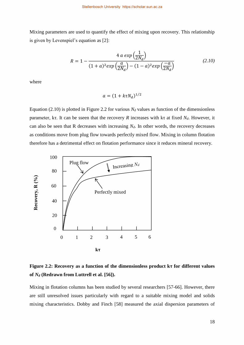
18
Mixing parameters are used to quantify the effect of mixing upon recovery. This relationship
is given by Levenspiel’s equation as [2]:
𝑅 = 1 −4 𝑎 𝑒𝑥𝑝 (
12𝑁𝑑
)
(1 + 𝑎)2𝑒𝑥𝑝 (𝑎
2𝑁𝑑) − (1 − 𝑎)2𝑒𝑥𝑝 (
−𝑎2𝑁𝑑
) (2.10)
where
𝑎 = (1 + 𝑘𝜏𝑁𝑑)1 2⁄
Equation (2.10) is plotted in Figure 2.2 for various Nd values as function of the dimensionless
parameter, kτ. It can be sseen that the recovery R increases with kτ at fixed Nd. However, it
can also be seen that R decreases with increasing Nd. In other words, the recovery decreases
as conditions move from plug flow towards perfectly mixed flow. Mixing in column flotation
therefore has a detrimental effect on flotation performance since it reduces mineral recovery.
Figure 2.2: Recovery as a function of the dimensionless product kτ for different values
of Nd (Redrawn from Luttrell et al. [56]).
Mixing in flotation columns has been studied by several researchers [57-66]. However, there
are still unresolved issues particularly with regard to a suitable mixing model and solids
mixing characteristics. Dobby and Finch [58] measured the axial dispersion parameters of
20
40
60
80
100
0
1 2 3 4 5 6 0
Rec
overy
, R
(%
)
kτ
Perfectly mixed
Plug flow
Stellenbosch University https://scholar.sun.ac.za
19
large industrial columns as an initial step towards the development of a scale-up methodology
for flotation columns. Their work involved pulsed tracer tests using liquid and solid tracers
on 0.46 and 0.91 m square columns, each 13 m high. The axial dispersion coefficient of
solids (Ds) was found to be equal to the liquid dispersion coefficient (Dl). The axial
dispersion coefficient (in m2/s) was also found to be linearly dependent on column diameter
according to the following relationship:
𝐷𝑠 = 𝐷𝑙 = 0.063𝑑𝐶 (2.11)
Mavros [9] reviewed different liquid phase axial dispersion coefficient data available in the
literature. The existing correlations were tested and a new correlation covering data for
different column sizes was derived. The axial dispersion coefficient was found to be related
to the column diameter and superficial gas velocity according to the following expression:
𝐷 = (9.3𝑑𝐶 − 30.1)𝐽𝑔0.603 (2.12)
The expression was able to estimate the axial dispersion coefficient reasonably. However, the
expression does not account for the effect of the superficial liquid velocity and is only
applicable to a limited range of liquid superficial velocities.
Mavros and Daniilidou [10] performed residence time distribution measurements of the
liquid phase in four flotation columns with increasing diameters. The measurements were
presented and analysed according to the axial dispersion model. The mixing of the liquid
phase was studied systematically in order to determine the effect of the column diameter and
the superficial liquid and gas velocities on the mixing process. The dispersion number,
characterising mixing, was determined in flotation columns of internal diameters varying
from 2.5 to 11.0 cm and the results were compared with literature data to obtain the following
correlation:
𝑁𝑑 = 0.0194 𝑒𝑥𝑝 (0.267𝑑𝐶)𝐽𝑙−0.56 (2.13)
where Jl = superficial liquid velocity.
Their experimentally obtained dispersion number data indicated that mixing in a flotation
column depends mostly upon the column diameter and the superficial liquid velocity. For the
usual range of velocities, the narrower the column, the less mixed are its contents, since plug
flow conditions are approached. The larger the column is, the more mixed will be its contents
Stellenbosch University https://scholar.sun.ac.za
20
leading to intense recirculation phenomena. It was also observed that the gas velocity (Jg)
does not affect the dispersion number considerably, while liquid velocity (Jl) seems to have a
limiting effect. In other words, the effect of Jl will at some stage begin to diminish until a
limit is reached beyond which it will no longer have any effect on the liquid dispersion
number.
Mankosa et al. [63] investigated mixing in column flotation and used RTD data to derive
expressions relating column operating and design parameters to axial dispersion. These
authors found that the axial dispersion increased with increasing gas rate and column
diameter while an increase in either liquid flow rate or column length caused a decrease in
axial dispersion. Using dimensional analysis an expression was obtained in which the Peclet
number (Pe) is related to column flow rates and geometry as follows:
𝑃𝑒 = 0.7 [(𝐻 𝑑𝐶⁄ )0.63(𝑢𝑖 𝐽𝑔⁄ )0.5
] (2.14)
The above expression was found to be useful for a wide range of design and operating
parameters.
Yianatos and Bergh [65] measured the residence time distribution of the liquid and solid
particles in an industrial flotation column in order to compare the hydrodynamic behaviour of
the liquid and mineral phases. The residence time of liquid (or fine particles) was found to be
about half the residence time of the coarse particles. It was also confirmed that the solids and
liquid axial dispersion coefficients were equal.
Yianatos et al. [66] evaluated the mixing characteristics and the effective residence time of
liquid and solid particles in industrial flotation equipment including mechanical cells and
flotation columns. In their work the mixing characteristics in flotation columns were
modelled using the Axial Dispersion Model (ADM) and the Large and small tanks in series
model (LSTS). The LSTS model consists of one large perfect mixer in series with two small
perfect mixers plus a dead time. The two small perfect mixers correspond to the feed input
and bubble generation zones while the large perfect mixer is related to volume extending
from below the feed enterance to the bubble generation level.
The analytical solution of this model was given by Yianatos et al. [66]. The LSTS model was
found to provide a more adequate description of the liquid mixing in flotation columns
compared to the ADM (using closed-closed boundaries). It was also found that despite the
Stellenbosch University https://scholar.sun.ac.za
21
presence of baffles, the mixing conditions in industrial columns are close to well mixed.
Their results further showed that the vessel dispersion number for the solid particles was
similar with the liquid one. However, the overall solids residence time was 11% smaller than
the liquid one despite the fact that the average particle size was finer (25% w/w with particle
sizes > 24 µm). These observations are similar to earlier findings by Dobby and Finch [58]
and Yianatos and Bergh [65].
Massinaei et al. [67] studied the mixing conditions in industrial rougher columns using
residence time distribution (RTD) data. They used a radioactive liquid tracer (Br-82) to trace
the material reporting to tailings and concentrate streams. It was found from the RTD
analysis that the large and small tanks in series (LSTS) model was the best model for
representing the liquid transferred to tailings while the N perfect mixers in series model best
represented the liquid going to the concentrate stream. A theoretical model for counter-
current columns was used to estimate the solids mean residence time. The results obtained
showed a ratio of 1.4:1 between the liquid and solids residence times. This work also showed
that despite the presence of vertical baffles in the columns, the mixing conditions were close
to well mixed.
Massinaei et al. [67] further described the possible causes of mixing in industrial columns.
Mixing or turbulence in industrial flotation columns was attributed to convective pulp
recirculation and turbulent dispersion resulting from the counter-current contact between the
bubble swarm and the pulp. The feed and air entrances also cause mixing near the top and
bottom parts of the column, respectively. In addition, operating variables can also affect the
mixing conditions in an industrial flotation column. For example, increasing the superficial
gas velocity may result in increase in the extent of mixing in the column while increasing the
pulp density will result in a reduction in the degree of mixing.
2.4 CFD models of column flotation in the literature
The use of mathematical modelling in research aimed at achieving improvements in mineral
processing and extractive metallurgy has been growing in importance. The models that are
being applied for this purpose range in complexity from those based on statistical regression
of experimental data (empirical models) to detailed micro-phenomenological models
representing all the physical and chemical phenomena associated with the process being
modelled [68].
Stellenbosch University https://scholar.sun.ac.za

22
In linear regression models, the process performance criteria are expressed as simple linear
functions of the process variables. However, such empirical models are usually case sensitive
and cannot be extrapolated beyond the range of data from which the model was derived.
Inspite of these limitations, empirical models have very useful features: they are easy to
construct, easy to apply, and they provide helpful information about the process which can be
used to develop more general models [69]. On the other hand, phenomenological models
provide a realistic representation of the process and are capable of being extrapolated. The
information required to develop this type of models can be obtained by means of fluid flow
simulation using Computational Fluid Dynamics (CFD) modelling [68].
Computational Fluid Dynamics (CFD) can be described as the study of fluid flow, heat
transfer and related phenomena using computer-based numerical simulations. CFD is based
on a set of governing equations derived from the laws of conservation of mass, momentum,
and energy. These equations form a system of non-linear partial differential equations (PDEs)
which usually have no analytical solutions. Numerical methods are therefore needed to solve
the governing equations in CFD simulations.
The derivation of these equations can be found in several texts such as Anderson [70] and
Versteeg and Malalasekera [71]. As described by Anderson [70], CFD involves replacement
of the partial differential equations with discretized algebraic equations that approximate the
partial differential equations. These algebraic equations are then solved to obtain flow field
values at discrete points in space and/or time. The discrete points define the grid or mesh of
the solution. The process of developing a set of algebraic equations that can be used in place
of partial differential equations is known as discretization. The algebraic equations are then
solved at discrete points in the flow domain.
Over the last few years, CFD has emerged as a powerful tool that can be used to predict the
complex hydrodynamics as well as the performance of mineral flotation cells. In CFD
modelling, the flotation cell is discretized into finite control volumes or grid cells where local
values of flow field variables are calculated. The detailed understanding of flow physics that
is achieved by using this method allows modifications to existing equipment and operating
conditions to improve flotation performance.
Mineral flotation is a multiphase process involving three phases: liquid, air bubbles, and
mineral particles. Multiphase models are therefore required in order to carry out CFD
simulations of a flotation cell. Some of the most widely used multiphase models include the
Stellenbosch University https://scholar.sun.ac.za
23
Eulerian-Lagrangian, the Eulerian-Eulerian, and the Volume-of-fluid (VOF) models. In the
Eulerian-Lagrangian approach, the liquid phase is modelled as a continuum while the
dispersed phase is modelled by tracking the individual trajectories of a large number of
particles. This approach is therefore limited to systems with a low volume fraction of
dispersed particles.
On the other hand, the Eulerian-Eulerian modelling approach treats all the different phases as
continuous phases. The momentum and continuity equations are then solved for each phase
separately. The Eulerian-Eulerian model can be applied to simulate very complex flows.
However, it does not always give the best results since empirical information is required to
close the momentum equations [72].
The VOF model is a Eulerian-Eulerian model in which the interface between the different
phases is tracked. The model can be used to simulate stratified flows, free surface flows, and
the movement of large bubbles in a liquid phase. Since the interface between the fluids must
be resolved, the VOF model is not suitable for a system with a large number of bubbles.
Despite CFD being one of the most widely used numerical modelling methods, literature on
CFD modelling of column flotation is rather scarce. One of the earliest CFD models of
column flotation was reported by Deng et al. [11] who presented a two-dimensional, two-
phase, fluid dynamic model of a flotation column. The model was used to simulate liquid and
gas flow patterns in the collection zone of the column using the MAC (Marker and Cell)
numerical method. The numerical computations were performed only for one half of the
column since the system was assumed to be axis-symmetric. The simulated liquid axial
velocity profile revealed a liquid circulation flow pattern in which the liquid flows upwards in
the center part of the column and downwards near the column walls. This study further
concluded that liquid mixing in flotation columns was primarily caused by the liquid
circulation resulting from gas flow rather than dispersion. However, only laminar flow was
considered in the study hence the model did not consider the effect of turbulent fluctuations
or turbulent eddies on liquid mixing in the column. Moreover, the actual mixing
characteristics of the column were not investigated in terms of residence time distribution
simulations. The model was also not validated with experimental data due to limited
published results at the time of their work.
Subsequent CFD based models of column flotation have been published focusing on different
aspects of the process. Building upon the work of Deng et al. [11], a two-dimensional Euler-
Stellenbosch University https://scholar.sun.ac.za
24
Lagrangian model was used by Xia et al. [15] to simulate the alleviation of liquid back-
mixing by baffles and packings in a flotation column. These authors studied the liquid flow
patterns in three different column geometries in order to compare the liquid back-mixing in
an open column, a horizontally perforated plate baffled column, and a regular structured
packed column. The simulated results revealed that the liquid back-mixing effect in bubble
columns could be alleviated using baffles or packings. In addition, the effects of operating
conditions such as uneven aeration, gas velocity, and bubble size on liquid flow patterns in
the column were also studied. A decrease in bubble size was reported to have caused an
increase in the upward axial liquid velocity resulting in a possible increase in liquid back-
mixing in the column. However, similar assumptions were applied as in Deng et al. [11]
where turbulence effects were not considered. The actual mixing processes in terms of liquid
RTD were also not included in the simulations.
A similar study was also conducted by Rehman et al. [17] who investigated the effect of
various perforated baffle designs on air holdup and mixing in a flotation/bubble column using
CFD. To reduce the computational cost, simulations were performed only for one quarter of
the column geometry using a rotational periodic boundary condition to periodically repeat the
results for the entire column. The Eulerian-Eulerian multiphase model was utilized in the
simulations together with the standard k-epsilon turbulence model. The trays (baffles) were
observed to significantly increase the overall air holdup compared to the column without
baffles. A similar observation was also reported by Xia et al. [15] who suggested that the
presence of baffles and packing would hinder the upward movement of bubbles and therefore
increase the bubble retention time or gas holdup. Rehman et al. [17] further reported a slight
decrease in gas holdup with height or axial direction which was attributed to the increase in
bubble size as a result of reduction in static pressure. However, this trend is quite the opposite
of the well known axial increase in gas holdup that has been previously reported by several
researchers [18, 30, 45, 73].
Another study was conducted by Chakraborty et al. [14] in which the effect of air flow rate,
height-to-diameter ratio, column taper angle, and sparger configuration on the hydrodynamics
of the column flotation cell was investigated. The Eulerian-Eulerian or two fluid model was
was employed to simulate the gas-liquid two phase flow in the column while turbulence in
the continuous phase was modelled using the well known single phase standard k-ϵ
turbulence model. In addition, the model suggested by Sato and Sekoguchi [74] was used to
account for bubble induced turbulence. This study concluded that increasing air flow rate
Stellenbosch University https://scholar.sun.ac.za
25
resulted in an increase in gas holdup and complexity in the bubble plume structure. In
addition, increasing column height-to-diameter ratio was also observed to bring about a
complex flow pattern with multiple staggered vortices in the column. A low height-to-
diameter ratio was therefore recommended as one of the required conditions for obtaining
good separation in a column flotation cell. However, previous studies [63] have also reported
that increasing height-to-diameter ratio actually results in a decrease in axial mixing in the
column. Increasing column height-to-diameter ratio will therefore result in improved
recovery and performance of the column. In terms of the effect of sparger configuration, the
work by Chakraborty et al. [14] found that uniform gas distribution was essential for column
flotation. Xia et al. [15] also recommended uniform aeration across the cross section of the
column.
Other recent CFD models of column flotation have focussed more on bubble-particle
interactions such as collision, attachment and detachment processes in the collection zone of
flotation columns. Some of the research reported in this category include the work by
Nadeem et al. [16]. and Koh and Schwarz [13]. Nadeem et al. [16] presented their work on
CFD simulation of bubble-particle collision probabilities in quiescent flotation conditions
similar to the conditions prevailing in column flotation. The simulations were conducted
using an Euler-Lagrange approach in which the velocity field was solved for steady state
conditions. The solid particles were introduced as a discrete phase injection and the
subsequent particle tracks were used to calculate collision probabilities. Turbulence was
modeled for the continuous phase using the standard k-ϵ turbulence model. The bubble-
particle collision probability was then modeled in a small rectangular geometry with a
stationary bubble positioned at its centre. A trap boundary condition was applied on the
bubble in order for the particles to become trapped upon collision. The collision probability
was then obtained as the ratio of trapped particles to the total number of particles. An
important finding of Nadeem et al. was that the probability of collision was higher for a
smaller (1 mm) bubble than for a larger (1.5 mm) bubble.
Koh and Schwarz [13] studied hydrodynamics in coal flotation using computational fluid
dynamics. They applied an Eulerian-Eulerian multi-fluid model to simulate a microcel
column and a Jameson cell using the CFD code CFX-4.4. The standard k-ϵ turbulence model
was used to model turbulence in the continuous pulp phase. The flotation effect was modeled
by considering three sub-processes including collision, attachment, and detachment. A
significant finding of their work was that the local particle-bubble detachment rate was
Stellenbosch University https://scholar.sun.ac.za
26
determined by the local value of the turbulent dissipation rate. The importance of identifying
those regions of high turbulent dissipation rates was therefore highlighted by these authors.
In a recently published paper, Sarhan et al. [75] have studied the impact of the presence of
solid particles on bubble coalescence and breakup in column flotation using Computational
Fluid Dynamics (CFD). They employed the commercial CFD software package AVL FIRE
2009.2 to model the hydrodynamics in the flotation column cell. The two-fluid or Eulerian-
Eulerian multiphase model was used together with the standard k-ϵ turbulence model which
was used for calculating the turbulent viscosity in the continuous (liquid) phase. In addition,
the population balance equation (PBE) was used to predict the number density of different
bubble size classes in the column. This study found that the presence of solids reduced the
gas holdup in the flotation cell (column). The authors also reported that the size of gas
bubbles decreased with increasing superficial gas velocity causing the gas holdup to increase.
Their results further showed that the sauter mean bubble diameter decreased with increasing
solids concentration.
The CFD models of column flotation discussed above have all focussed on the processes
occurring in the collection zone of the column. However, some CFD models of froth
behaviour in flotation cells are also available in the literature [23, 76]. Cilliers [23] presented
a paper in which the use of CFD in foam and froth modelling was discussed. The paper
included an introduction of the physics of froths and a review of the methodology of
combining the models for each phase into a complete description. An example of the use of
froth CFD for equipment design was also given in which two alternative methods of wash
water addition were compared. The paper concluded by highlighting a number of issues that
still need to be addressed, in particular, the failure of bubble films causing coalescence in the
froth and the bursting of bubbles on the surface. Cilliers [23] further observed that the
combination of pulp and froth models into a single simulation was desired but difficult to
accomplish due to the differences in turbulence and flow behaviour, and the complex mass
transfer across the pulp-froth interface.
A more recent publication [76] describes a numerical model for the flow of foams in flotation
cells that can be used to simulate flowing foams in up to three-dimensions. The numerical
model was implemented in fluidity, a general purpose finite element method code that allows
simulations to be carried out on anisotropic unstructured meshes. The code makes use of the
finite elements to solve Laplace’s equation for a potential function and is capable of using
Stellenbosch University https://scholar.sun.ac.za
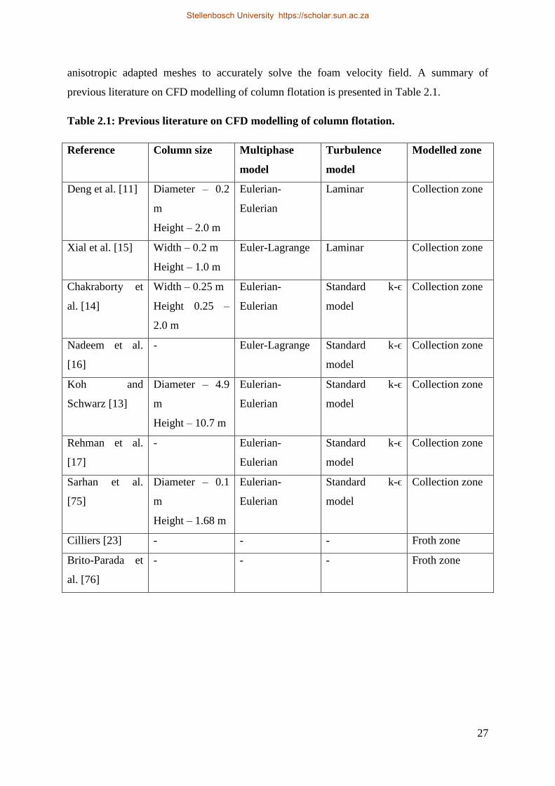
27
anisotropic adapted meshes to accurately solve the foam velocity field. A summary of
previous literature on CFD modelling of column flotation is presented in Table 2.1.
Table 2.1: Previous literature on CFD modelling of column flotation.
Reference Column size Multiphase
model
Turbulence
model
Modelled zone
Deng et al. [11] Diameter – 0.2
m
Height – 2.0 m
Eulerian-
Eulerian
Laminar Collection zone
Xial et al. [15] Width – 0.2 m
Height – 1.0 m
Euler-Lagrange Laminar Collection zone
Chakraborty et
al. [14]
Width – 0.25 m
Height 0.25 –
2.0 m
Eulerian-
Eulerian
Standard k-ϵ
model
Collection zone
Nadeem et al.
[16]
- Euler-Lagrange Standard k-ϵ
model
Collection zone
Koh and
Schwarz [13]
Diameter – 4.9
m
Height – 10.7 m
Eulerian-
Eulerian
Standard k-ϵ
model
Collection zone
Rehman et al.
[17]
- Eulerian-
Eulerian
Standard k-ϵ
model
Collection zone
Sarhan et al.
[75]
Diameter – 0.1
m
Height – 1.68 m
Eulerian-
Eulerian
Standard k-ϵ
model
Collection zone
Cilliers [23] - - - Froth zone
Brito-Parada et
al. [76]
- - - Froth zone
Stellenbosch University https://scholar.sun.ac.za

28
2.5 Conclusion
This literature review has discussed the established body of knowledge regarding gas
dispersion and mixing characteristics of flotation columns. Previous CFD models of column
flotation available in the published literature have also been reviewed. The various
approaches that have been used to model column flotation are outlined in Table 2.1. Most of
the researchers have used the Eulerian-Eulerian multiphase model together with the standard
k-ϵ turbulence model to simulate the multiphase flows in the flotation column while others
have assumed that turbulence was insignificant. It would therefore be instructive to
investigate the effect of the different turbulence models in the context of column flotation
modelling. However, this might not be possible to do in the present research due to lack of
detailed experimental data against which the various models can be compared.
Despite the fact that a number of CFD models have already been reported by previous
researchers, this literature review has found that gas dispersion and mixing in column
flotation have not been adequately studied. For example, the only study in which the axial gas
holdup is investigated reported profiles that contradict the well known axial increase in gas
holdup along the column axis [17]. On the other hand, while both Deng et al. [11] and Xia et
al. [15] discuss mixing in column flotation, the actual mixing in the column in terms of RTD
studies has not been simulated. The conclusions that were made in these studies regarding
back-mixing in column flotation were therefore based entirely on the effects of various
operational or geometrical conditions on the axial liquid velocity profiles. However, it would
be more informative to investigate the effect of operating parameters (such as superficial gas
velocity or bubble size) or column geometry on the actual liquid mixing parameters such as
the vessel dispersion or axial dispersion coefficient. In addition, the work conducted by Deng
et al. [11] and Xia et al. [15] was limited to two phase (gas-liquid) flow in which mineral
particles were not considered. The mixing characteristics of solids in column flotation have
therefore not been studied in the previous CFD models.
Considering the gaps established in this literature review, the purpose of the present research
is to apply CFD methodology to investigate the gas dispersion and mixing chacteristics of
pilot and industrial scale flotation columns. In terms of gas dispersion parameters, CFD will
be applied to simulate the average gas holdup and the axial gas holdup variation in a pilot
column flotation cell. The effect of gas rate and flow regime on radial gas holdup profiles
will be investigated in the context of the maximum superficial gas velocity for column
flotation. On the other hand, the mixing parameters in column flotation will be studied with
Stellenbosch University https://scholar.sun.ac.za

29
particular interest on the solids mixing characteristics and the effects of particle and bubble
sizes on the liquid dispersion number.
Stellenbosch University https://scholar.sun.ac.za
30
Chapter 3 Simulation Methodology
3.1 Introduction
This chapter provides the details of the methodology that will be employed in this thesis. The
aim of the research, namely to apply CFD simulations to investigate gas dispersion and
mixing in flotation columns has been established in the literature review in the previous
chapter (Chapter 2). The focus of this methodology chapter is therefore on the development
of a CFD methodology that is capable of providing reliable predictions of the gas dispersion
and mixing parameters in the column. In general, CFD simulations involve the following six
aspects:
defining a representative model geometry and boundary conditions for the equipment
that is to be modelled
meshing the model geometry in order to generate a grid of cells in which flow
variables will be calculated
selecting suitable modelling approaches for computing the turbulent multiphase flow
problem under study
Setting up the solver solution methods for the computation
Solving the corresponding partial differential equations for the flow variables
Analysing the results
This chapter is therefore laid out in such a way that these six themes are addressed in the
flotation column CFD model.
3.2 Model geometry, mesh and boundary conditions
3.2.1 Defining the computational domain
Flotation columns are divisible into two distinct zones as described in Chapter 1, the
collection zone and the cleaning zone. Since the two zones have different hydrodynamic
characteristics, the definition of a relevant computational domain is essential to the
simulation of flotation columns. In as much as it would be desirable to formulate CFD
simulations that combine the two zones, their inherent differences in the flow and turbulence
characteristics would make it difficult to combine the two zones together in a single
simulation [23]. In addition, such a CFD model would have to account for the complex mass
transfer processes occurring accross the interface between the two zones.
Stellenbosch University https://scholar.sun.ac.za

31
Previous studies have either simulated the collection zone or the froth zone as described in
the literature review. The present model therefore considers the collection zone of the
columns while the froth zone is not modelled. The resulting simplified model geometry is a
vessel of height equal to the collection zone height and radial dimensions similar to the
respective industrial or pilot column being simulated.
3.2.2 Modelling of the spargers
The sparging of gas was modelled by means of mass and momentum source terms for the
computational cells at the bottom of the column. The model assumes that the gas phase enters
the column in form of air bubbles. Since the sparging systems that are used in industrial
flotation columns are designed to achieve uniform distribution of air bubbles over the entire
column cross section [26], the air bubbles were introduced over the entire column cross
section in the present research without including the physical spargers in the model geometry.
Uniform air distribution has also been verified in pilot scale flotation columns by means of
radial gas holdup measurements [27, 28]. The use of the entire column cross section for
bubble introduction into the column is therefore a legitimate albeit simplified representation
of the sparging system in the simulated columns. Correspondingly, the information available
in the literature for the simulated flotation columns was mostly presented in terms of
superficial velocities calculated over the entire column cross-section.
3.2.2.1 Calculation of mass and momentum source terms
The mass and momentum source terms were calculated from the superficial gas (air) velocity,
Jg as follows:
𝑀𝑎𝑠𝑠 𝑠𝑜𝑢𝑟𝑐𝑒 =
𝜌𝑎𝑖𝑟 ∗ 𝐴𝑐 ∗ 𝐽𝑔
𝑉 (3.1)
where ρair is the density of air (1.225 kg/m3), Ac is the column cross-sectional area (m2), Jg is
the superficial gas (air) velocity (m/s) and V is the volume of the cell zone where the source
terms are applied. The momentum source terms were calculated from the respective mass
source terms according to the following equation:
𝑀𝑜𝑚𝑒𝑛𝑡𝑢𝑚 𝑠𝑜𝑢𝑟𝑐𝑒 = 𝑚𝑎𝑠𝑠 𝑠𝑜𝑢𝑟𝑐𝑒 ∗ 𝐽𝑔 (3.2)
In this study, the air bubbles are assumed to emerge from the sparger in the upward direction.
The momentum source terms were therefore introduced in the upward direction, in other
words, only the Y momentum component was considered while the X and Z momentum
Stellenbosch University https://scholar.sun.ac.za
32
components were neglected. The calculated mass and momentum source terms for the
different columns simulated in this research are provided in Appendix 1 and 3.
3.2.3 Boundary conditions
3.2.3.1 Batch operated columns
For the batch operated column, there are no inlets or outlets for the liquid phase. Boundary
conditions were therefore specified for the column wall only. In this case, no slip boundary
conditions were applied at the column wall for both the continuous phase (water) and the
dispersed phase (air bubbles).
3.2.3.2 Continuously operated columns
For the continuously operated column, inlet and outlet boundary conditions had to be
specified at the top (inlet) and bottom (outlet) of the column. For the liquid phase the top of
the column was modelled as a velocity inlet boundary where inlet velocity was set equal to
the superficial liquid velocity, Jl. Since the computational domain being considered is the
collection zone of the column, the superficial liquid velocity must include the feed rate plus
the bias water resulting from wash water addition. The superficial liquid velocity is therefore
equal to the superficial tailing rate. The bottom part of the column was also modelled as
velocity inlet boundary where exit velocity was set equal to superficial liquid velocity but
with a negative sign. For the column wall, no slip conditions were applied a for both the
liquid (continuous phase) and the air bubbles as well as solids (dispersed phases).
3.2.4 Mesh size and grid independence considerations
In order to eliminate the possibility of errors resulting from coarse mesh sizes, grid
dependence studies were undertaken in which the mesh was progressively refined from an
initially coarse mesh until there was no significant change in the simulated axial water
velocity and bubble velocity profiles.
3.3 Multiphase model
3.3.1 Overview of multiphase models
The models for simulating multiphase flows can generally be grouped into three classes:
Direct Numerical Simulation (DNS)
Eulerian-Lagrangian
Eulerian-Eulerian
Stellenbosch University https://scholar.sun.ac.za
33
Direct numerical simulations (DNS) can be used to obtain a full resolution of the behaviour
of bubbles or particles in a carrying fluid. Multiphase DNS therefore involves simulations in
which one fully resolves the temporal and spatial scales relevant to the fluid dynamics [77].
One of the most widely used methods in multiphase DNS is the Volume of Fluid (VOF)
method. In the VOF model the interface between the different phases is tracked. The VOF
model is suitable for simulating stratified flows, free surface flows and the movement of large
bubbles in a liquid [78]. Since the interface between the phases must be resolved, VOF is not
applicable for systems with a large number of bubbles or liquid droplets.
In the Eulerian-Lagrangian modelling method, the continuous phase is modelled as a
continuum by solving the Navier-Stokes equations. On the other hand, the dispersed
(secondary) phase is simulated in a Lagrangian frame of reference by tracking the motion of
the individual particles (or bubbles) using an equation of motion. However, the computational
cost associated with computing individual particle or bubble trajectories is high and increases
with an increase in the number of simulated particles. The Eulerian-Lagrangian method is
therefore limited to dilute systems in which the dispersed phase volume fraction is less than
10% [78, 79].
In the Eulerian-Eulerian modelling approach, the different phases are considered as
continuous phases that are interacting with each other. Conservation equations governing the
balance of mass, momentum, and energy are in this case solved for each phase separately.
However, the interaction between the different phases must be accounted for through
additional models.
3.3.2 Choice of multiphase model for the present research
The multiphase CFD model used in this research was selected after a thorough literature
review of CFD models of bubble column reactors and flotation columns. The ‘hierarchy of
models’ concept that was introduced by Delnoij et al. [80] was particularly useful in the
selection of a suitable multiphase model for industrial and pilot scale flotation columns.
A range of hydrodynamic phenomena characterised by different length and time scales occur
in bubble columns. In addition, a wide range of bubble diameters and shapes can also be
encountered depending on the physical properties of the liquid phase and the flow regime in
which the bubble column is being operated. Bubble columns also differ in sizes and
geometry. It is, therefore, difficult to develop a generalized CFD model that is capable of
Stellenbosch University https://scholar.sun.ac.za

34
resolving all the different hydrodynamic features occurring at the various length and time
scales.
The ‘hierarchy of models’ concept recommends different CFD models depending on the size
of the column, the length scales of the particular hydrodynamic phenomena, and the
prevailing flow regime. In other words each model is applied for studying specific
hydrodynamic phenomena, occurring at a defined scale [81].
According to Delnoij et al. [80] a two-fluid model is recommended to study flow structures
occurring in industrial scale bubble columns due to its relatively lower computational cost.
An Eulerian-Eulerian two-fluid model was therefore chosen in the present research
considering the size of the simulated flotation columns. The Eulerian-Eulerian approach has
been applied in several CFD models of pilot-scale bubble columns [22, 32, 82] of similar
dimensions as the flotation columns that are simulated in the present research. A review of
previous CFD models involving column flotation also found that the Eulerian-Eulerian model
was used in most of these studies[11, 13, 14, 17].
3.3.3 Eulerian-Eulerian multiphase model
In the Eulerian-Eulerian approach, both the continuous (primary) phase and the dispersed
(secondary) phase are modelled in an Eulerian frame of reference as interpenetrating
continua. The gas, solid, and liquid phases are considered as three distinct phases that are
interacting with each other. Conservation equations for mass and momentum are therefore
solved for each phase separately. Interaction between the phases is then accounted for by
means of momentum exchange terms incorporated in their respective momentum equations.
In the present research, the multiphase flow in the flotation columns was modelled
considering water as the continuous phase (or primary phase) while air bubbles and solid
particles were treated as dispersed phases (or secondary phases). The volume averaged mass
and momentum conservation equations are as follows, respectively:
𝜕
𝜕𝑡(휀𝑞𝜌𝑞) + 𝛻. (휀𝑞𝜌𝑞𝒖𝑞⃗⃗ ⃗⃗ ) = 𝑆𝑞 (3.3)
𝜕
𝜕𝑡(휀𝑞𝜌𝑞𝒖𝑞⃗⃗ ⃗⃗ ) + 𝛻. (휀𝑞𝜌𝑞𝒖𝑞⃗⃗ ⃗⃗ ⊗ 𝒖𝑞⃗⃗ ⃗⃗ ) = −휀𝑞𝛻𝑝 + 𝛻. 휀𝑞𝜏𝑞̿̿̿ + 휀𝑞𝜌𝑞�⃗⃗� + 𝑀𝐺,𝐿 (3.4)
where q is the phase indicator, q = L for the liquid phase, q = G for the gas phase, εq is the
volume fraction, ρq is the phase density, and uq is the velocity of the qth phase, while Sq is a
Stellenbosch University https://scholar.sun.ac.za

35
source term. 𝑀𝐺,𝐿 is the interaction force between the phases and ερg is the gravity force,
while τq̿ is the qth phase stress-strain tensor given by:
𝜏𝑞̿̿̿ = 휀𝑞𝜇𝑞(𝛻𝒖𝑞⃗⃗ ⃗⃗ + 𝛻𝒖𝑞⃗⃗ ⃗⃗
𝑇) + 휀𝑞 (𝜆𝑞 −
2
3𝜇𝑞)𝛻. 𝒖𝑞⃗⃗ ⃗⃗ 𝐼 ̿ (3.5)
The liquid phase was modelled as incompressible hence its continuity (mass conservation)
equation is simplified as follows:
𝜕휀𝐿
𝜕𝑡+ ∇. (휀𝐿𝜌𝐿𝒖𝐿⃗⃗ ⃗⃗ ) = 0 (3.6)
Interaction between the phases is generally accounted for through inclusion of the drag force
while non drag forces such as the virtual mass and lift force can be neglected [83-85].
Momentum exchange between the phases was therefore accounted for by means of the drag
force only in this research. The different drag models that have been used in this research are
described in subsequent chapters.
3.4 Turbulence model
3.4.1 Overview of turbulence modelling methods
Turbulent flows are characterised by velocity fluctuations in which small scale and high
frequency fluctuations may occur. It would therefore be too computationally expensive to
simulate turbulent flows in detail, especially for high Reynolds number flows. Fortunately, it
is not always necessary in most engineering applications to resolve all the details of the
turbulent fluctuations. Instead, the small scale and high frequency fluctuations can be
removed by manipulating the instantaneous (exact) governing equations to produce modified
equations that are computationally less expensive to solve. However, the modified equations
contain additional unknown variables that have to be determined using turbulence models.
The choice of turbulence model is crucial for successful CFD simulations. There are
numerous turbulence models that have been proposed over the last few decades. In order to
select a suitable turbulence model, one has to consider the type of flow that is to be modelled
as well as its implications on the computational cost of the simulations. Selecting a particular
turbulence model is therefore usually a trade-off between the required accuracy and the
computational cost of the simulations.
Stellenbosch University https://scholar.sun.ac.za
36
The methods for turbulence modelling can be grouped in to three categories: Direct
numerical simulation (DNS), Large-eddy simulation (LES), and Reynolds-averaged Navier-
Stokes (RANS) equations. In DNS, the unsteady 3D Navier-Stokes equations are solved
directly to resolve the turbulent flow. A turbulence model is therefore not required since the
equations adequately describe the flow. However, DNS requires very dense computational
grids and small time steps in order to resolve the entire range of length scales and time scales
of the turbulent flow, especially at high Reynolds number. The computational cost of DNS is
therefore too high for the method to be applied for industrial computations [71, 78].
On the other hand, Large-eddy simulation (LES) is another form of modelling approach
which is less computationally expensive than DNS. In LES, the dynamics of the large
turbulent eddies are computed while the smallest scales of the turbulence are unresolved. This
is accomplished by space filtering of the unsteady Navier-Stokes equations to separate the
larger eddies and eliminate the smaller eddies prior to the computations. The effects of the
small unresolved eddies on the resolved flow (mean flow and large eddies) are then included
by means of a sub-grid scale model. Since a coarser mesh is used in LES simulations than the
mesh required for DNS, LES results in substantial savings in the computational cost of the
simulations. However, LES simulations also require a very fine mesh and small time steps.
The computational cost of LES is therefore still high compared with other turbulence models.
The most widely used turbulence models for routine engineering simulations are based on the
Reynolds-averaged Navier-Stokes (RANS) equations. In this approach, the instantaneous
Navier-Stokes equations are time-averaged to produce the RANS equations which are solved
to obtain a time averaged or mean flow field. The RANS equations are derived by
decomposing the instantaneous variables in the Navier-Stokes equations into a mean part and
a fluctuating component and then time averaging the resulting equations to obtain a set of
equations for the average flow field (RANS equations). The velocity components are
decomposed into a mean part and a fluctuating component according to:
𝑢𝑖 = 𝑢𝑖 + 𝑢𝑖′ (3.7)
where 𝑢𝑖 and 𝑢𝑖′ are the mean and fluctuating components, respectively (i = 1, 2, 3).
Similarly, the scalar quantities such as pressure and energy are decomposed into the
following form:
𝜑 = 𝜑 + 𝜑′ (3.8)
Stellenbosch University https://scholar.sun.ac.za
37
where 𝜑 represents any scalar quantity.
Substituting the decomposed form for the flow variables into the continuity and momentum
equations (Navier-Stokes equations) and taking the time average produces the RANS
equations. However, the Reynolds-averaged momentum equations contain additional
unknowns (−𝜌𝑢𝑖′𝑢𝑗
′) called Reynolds or turbulent stresses which represent the effects of
turbulent fluctuations on the mean flow. The Reynolds stresses are subsequently determined
with the help of a turbulence model. RANS turbulence modelling therefore involves the
calculation of the mean flow while employing turbulence models to simulate the effect of
turbulent fluctuations on the mean flow. RANS turbulence models are classified according to
the number of additional transport equations that need to be solved together with the
Reynolds averaged flow equations as outlined in Table 3.1 [71].
Table 3.1: RANS based turbulence models.
Number of additional transport equations Turbulence model
Zero Mixing length model
One Sparlart – Allmaras model
Two k-ϵ model
k-ω model
Algebraic stress model
Seven Reynolds stress model
3.4.2 Choice of turbulence model for the present research
The turbulence model used in this research was selected following a thorough literature
survey on CFD modelling of column flotation cells. Most of the studies have utilised the
standard k-ϵ turbulence model to simulate turbulence in the continuous (liquid) phase [13, 14,
16, 86, 87] while others have assumed laminar flow conditions [11, 15]. However, the
presence of turbulence resulting from bubble motion and the feed and air enterances near the
top and bottom of the column has been suggested as the cause of the dispersion which is one
of the reasons for mixing in flotation columns [66, 67, 88]. It is therefore necessary to
consider turbulence in subsequent CFD models of column flotation.
For flows with recirculation, such as the flows encountered in flotation columns, the
realizable k-ϵ turbulence model has been reported to perform better than the widely used
Stellenbosch University https://scholar.sun.ac.za

38
standard k-ϵ model [89]. The present research therefore employs the realizable k-ϵ turbulence
model to account for turbulence in the continuous phase (water).
3.4.3 Realizable k-ϵ turbulence model
The k-ϵ model is based on the Eddy Viscosity concept. The Reynolds stresses are therefore
related to the velocity gradients through the eddy or turbulent viscosity as presented in the
following equation:
−𝜌𝑢𝑖
′𝑢𝑗′ = 𝜇𝑡 (
𝜕𝒖𝑖
𝜕𝑥𝑗+
𝜕𝒖𝑗
𝜕𝑥𝑖) −
2
3(𝜌𝑘 + 𝜇𝑡
𝜕𝒖𝑘
𝜕𝑥𝑖) 𝛿𝑖𝑗 (3.9)
where μt is the eddy or turbulent viscosity, k is the turbulence kinetic energy and δij is the
Kronecker delta. The turbulent viscosity is then calculated from the turbulence kinetic energy
(k) and the turbulence dissipation rate (ϵ). The k-ϵ model is therefore a two equation
turbulence model since two additional transport equations must be solved for the turbulence
kinetic energy (k) and dissipation rates (ϵ). For the realizable k-ϵ model, the turbulence
kinetic energy (k) and turbulence dissipation rate equations are presented as follows:
𝜕
𝜕𝑡(𝜌𝑘) +
𝜕
𝜕𝑥𝑗(𝜌𝑘𝒖𝑗) =
𝜕
𝜕𝑥𝑗[(𝜇 +
𝜇𝑡
𝜎𝑘)
𝜕𝑘
𝜕𝑥𝑗] + 𝐺𝑘 + 𝐺𝑏 − 𝜌𝜖 − 𝑌𝑀 + 𝑆𝑘 (3.10)
𝜕
𝜕𝑡(𝜌𝜖) +
𝜕
𝜕𝑥𝑗(𝜌𝜖𝒖𝑗)
=𝜕
𝜕𝑥𝑗[(𝜇 +
𝜇𝑡
𝜎𝜖)
𝜕𝜖
𝜕𝑥𝑗] + 𝜌𝐶1𝑆𝜖 − 𝜌𝐶2
𝜖2
𝑘 + √𝜈𝜖+ 𝐶1𝜖
𝜖
𝑘𝐶3𝜖𝐺𝑏 + 𝑆𝜖
(3.11)
where
𝐶1 = 𝑚𝑎𝑥 [0.43,
𝜂
𝜂 + 5] , 𝜂 = 𝑆
𝑘
𝜖, 𝑆 = √2𝑆𝑖𝑗𝑆𝑖𝑗 (3.12)
The quantities C1 and C1ϵ are empirical constants while σk and σϵ are the turbulent Prandtl
numbers for k and ϵ, respectively. Sk and Sϵ are source terms. The term Gk represents the
generation of turbulence kinetic energy due to velocity gradients while Gb is the turbulence
kinetic energy due to buoyancy. YM is the contribution of the fluctuating dilatation in
compressible turbulence to the overall dissipation rate. The eddy viscosity or turbulent
viscosity, μt is then modelled as follows:
Stellenbosch University https://scholar.sun.ac.za

39
𝜇𝑡 = 𝜌𝐶𝜇
𝑘2
𝜖 (3.13)
The variable, Cμ is calculated from the following equation:
𝐶𝜇 =
1
𝐴0 + 𝐴𝑠𝑘𝑈∗
𝜖
where
𝑈∗ ≡ √𝑆𝑖𝑗𝑆𝑖𝑗 + 𝛺𝑖�̃�𝛺𝑖�̃�
𝛺𝑖�̃� = 𝛺𝑖𝑗 − 2𝜖𝑖𝑗𝑘𝜔𝑘
𝛺𝑖𝑗 = 𝛺𝑖𝑗̅̅ ̅̅ − 𝜖𝑖𝑗𝑘𝜔𝑘
𝐴0 = 4.04
𝐴𝑠 = √6𝑐𝑜𝑠∅
∅ =1
3𝑐𝑜𝑠−1(√6𝑊),𝑊 =
𝑆𝑖𝑗𝑆𝑗𝑘𝑆𝑘𝑖
𝑆3, �̃� = √𝑆𝑖𝑗𝑆𝑖𝑗 , 𝑆𝑖𝑗 =
1
2(𝜕𝑢𝑗
𝜕𝑥𝑖+
𝜕𝑢𝑖
𝜕𝑥𝑗)
(3.14)
where 𝛺𝑖𝑗̅̅ ̅̅ is the mean rate of rotation rate viewed in a rotating reference frame with angular
momentum 𝜔𝑘. The model constants for the Realizable k-ϵ turbulence model are summarized
in Table 3.2.
Table 3.2: Turbulence model constants.
𝜎𝑘 𝜎𝜖 𝐶1 𝐶2 𝐶𝜇 𝐴0 𝐶1𝜖
1.0 1.2 Eq.(3.12) 1.9 Eq.(3.14) 4.0 1.44
3.4.4 Turbulence near the column wall
The presence of walls has a profound effect on the behaviour of turbulence in wall bounded
turbulent flows. The near wall region is characterised by relatively larger viscous effects and
rapid variation of the flow variables. Correct representation of the influence of walls on
turbulent flows is therefore an important aspect of CFD simulations involving wall-bounded
flows.
The near-wall region is divisible into three sublayers. In the innermost layer, the viscous
sublayer, flow is almost laminar and molecular viscosity has a dominant effect on momentum
transfer while turbulence plays a major role in the outer layer called the fully turbulent layer.
Between the viscous sublayer and the fully turbulent layer is an interim region in which the
Stellenbosch University https://scholar.sun.ac.za

40
molecular viscosity and turbulence are equaly important. This interim layer is known as the
buffer layer.
There are two main approaches that can be used to model the near wall region in CFD
simulations. In the first approach, the viscosity affected inner region (viscous and buffer
layers) is not resolved. Instead, semi-empirical formulae known as wall functions are used to
bridge the viscosity affected region between the wall and the fully turbulent region. This
approach saves considerable comuptational resources since the the viscosity affected near
wall region is not resolved. The wall function approach was therefore used in the present
research in order to minimise the computational cost of the simulations.
The standard wall functions used in this research are based on the work of Launder and
Spalding [90]. The momentum boundary condition is then obtained from the law-of-the-wall
for the mean velocity as follows:
𝑈∗ =
1
𝜅ln(𝐸𝑦∗) (3.15)
where U* is the dimensionless velocity and y* is the dimensionless distance from the wall.
These parameters are given by the following expressions:
𝑈∗ ≡ 𝑈𝑃𝐶𝜇1 4⁄ 𝑘𝑃
1 2⁄ (3.16)
𝑦∗ ≡
𝜌𝐶𝜇1 4⁄ 𝑘𝑃
1 2⁄ 𝑦𝑃
𝜇 (3.17)
In equations (3.15) to (3.17), κ is the Von Kármán constant (= 0.4187), E is an empirical
constant (= 9.793), UP is the mean velocity of the fluid at the near-wall node P, kP is the
turbulence kinetic energy at near-wall node P, yP is the distance from point P to the wall, and
μ is the dynamic viscosity of the fluid.
The second approach, the low Reynolds number model method, employs modified turbulence
models which are used to resolve the inner layer up to the wall. The wall function approach
and the low Reynolds number model approach are compared in Figure 3.1.
Stellenbosch University https://scholar.sun.ac.za
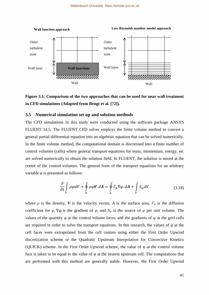
41
Figure 3.1: Comparison of the two approaches that can be used for near wall treatment
in CFD simulations (Adapted from Bengt et al. [72]).
3.5 Numerical simulation set up and solution methods
The CFD simulations in this study were conducted using the software package ANSYS
FLUENT 14.5. The FLUENT CFD solver employs the finite volume method to convert a
general partial differential equation into an algebraic equation that can be solved numerically.
In the finite volume method, the computational domain is discretised into a finite number of
control volumes (cells) where general transport equations for mass, momentum, energy, etc
are solved numerically to obtain the solution field. In FLUENT, the solution is stored at the
centre of the control volumes. The general form of the transport equations for an arbitrary
variable φ is presented as follows:
𝜕
𝜕𝑡∫𝜌𝜑𝑑𝑉
𝑉
+ ∮𝜌𝜑𝑽. 𝑑𝑨
𝐴
= ∮Γ𝜑∇𝜑. 𝑑𝑨
𝐴
+ ∫𝑆𝜑𝑑𝑉
𝑉
(3.18)
where ρ is the density, V is the velocity vector, A is the surface area, Γφ is the diffusion
coefficient for φ, ∇𝜑 is the gradient of φ, and Sφ is the source of φ per unit volume. The
values of the quantity φ at the control volume faces, and the gradients of φ at the grid cells
are required in order to solve the transport equations. In this research, the values of φ at the
cell faces were extrapolated from the cell centres using either the First Order Upwind
discretization scheme or the Quadratic Upstream Interpolation for Convective Kinetics
(QUICK) scheme. In the First Order Upwind scheme, the value of φ at the control volume
face is taken to be equal to the value of φ at the nearest upstream cell. The computations that
are performed with this method are generally stable. However, the First Order Upwind
Wall functions Wall layer
Outer
turbulent
zone
Wall
Wall function approach
Wall
Outer
turbulent
zone
Wall layer
Low Reynolds number model approach
Stellenbosch University https://scholar.sun.ac.za

42
scheme is prone to numerical diffusion errors since it has only first order accuracy in terms of
Taylor series truncation error (TSTE).
Alternatively, a higher order discretization scheme such as the QUICK scheme can be
employed in order to minimize numerical diffusion errors. In the QUICK scheme, the value
of φ at the cell face is obtained from a quadratic function passing through two bracketing
nodes (on each side of the face) and a node on the upstream side. For a uniform grid, the
value of φ at the cell face between bracketing nodes i and i – 1 and upstream node i – 2 is
given by [71]:
𝜑𝑓𝑎𝑐𝑒 =
6
8𝜑𝑖−1 +
3
8𝜑𝑖 −
1
8𝜑𝑖−2 (3.19)
In terms of Taylor series truncation error the QUICK scheme is third order accurate on a
uniform mesh. The pressure and the velocity components were coupled using the SIMPLE
algorithm in an iterative process outlined in Figure 3.2. The Computations were performed
using the University of Stellenbosch's Rhasatsha High Performance Computing (HPC)
cluster: http://www.sun.ac.za/hpc.
Stellenbosch University https://scholar.sun.ac.za
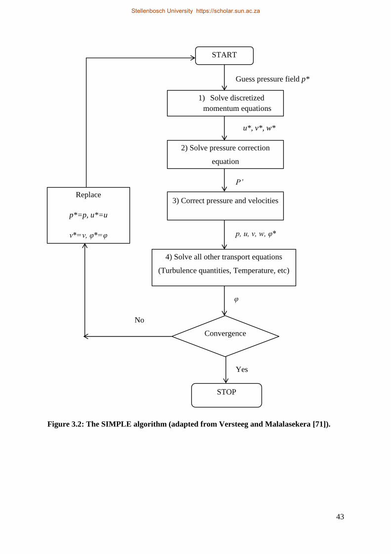
43
Figure 3.2: The SIMPLE algorithm (adapted from Versteeg and Malalasekera [71]).
START
Guess pressure field p*
1) Solve discretized
momentum equations
2) Solve pressure correction
equation
3) Correct pressure and velocities
4) Solve all other transport equations
(Turbulence quantities, Temperature, etc)
Convergence
?
STOP
Replace
p*=p, u*=u
v*=v, φ*=φ
u*, v*, w*
P’
p, u, v, w, φ*
φ
Yes
No
Stellenbosch University https://scholar.sun.ac.za
44
Chapter 4 Numerical prediction of gas holdup and its axial variation in a
flotation column
4.1 Introduction
In this chapter, Computational Fluid Dynamics (CFD) is applied to predict the average gas
holdup and the axial gas holdup variation in the collection zone of a 0.91 m-diameter
cylindrical pilot flotation column operated in batch mode. Gas holdup is one of the most
important parameters affecting the metallurgical performance of the column. It is defined as
the volumetric fraction (or percentage) occupied by gas at any point in a column [2]. Some
studies have reported that gas holdup affected both the recovery and grade in industrial and
pilot scale flotation columns [41, 42]. These studies reported a linear relationship between
gas holdup and recovery. Linear relationships between gas holdup and the flotation rate
constant have also been identified highlighting its effect on flotation kinetics [4, 43]. Other
researchers have suggested that gas holdup could be used for control purposes in column
flotation [44]. However, apart from its potential in control, gas holdup also has diagnostic
applications, for example, the sudden drop in gas holdup that occurs when a sparger is
damaged [44].
CFD modelling has been applied to predict the average gas holdup for the whole flotation
column [13, 14]. However, the gas holdup has been observed to vary with height along the
collection zone of the flotation column– increasing by almost 100% from the bottom to the
top of the column [18, 45, 73]. The increase in gas holdup with height has been attributed to
the hydrostatic expansion of bubbles [30, 73]
In spite of the reported increase in gas holdup along the column height, the CFD literature on
column flotation does not account for this phenomenon. This could result in the under-
prediction of gas holdup especially in cases where the available experimental measurements
were taken near the top of the column. In an attempt to understand the observed axial
variations in gas holdup, some researchers conducted experiments in which axial velocity
profiles of single bubbles were measured [31]. On the other hand CFD is capable of
predicting the entire flow fields of the various phases involved in the flotation process. The
axial variation in bubble velocity can therefore be investigated with CFD in order to
understand its relationship with the spatial gas distribution in the column.
Stellenbosch University https://scholar.sun.ac.za

45
The aim of the work discussed in this chapter was therefore to investigate the application of
CFD for predicting not only the average gas holdup but also the axial gas holdup variation in
the column. In this regard, CFD was used to model a cylindrical pilot column that was used
in previous studies on axial gas holdup distribution [18, 45]. In addition, the axial velocity
profiles of the gas phase were studied in order to explain the increase in gas holdup with
height along the column.
4.2 Description of the column
The pilot flotation column was used in previous research by Gomez et al. [18, 45] to study
gas holdup in the collection zone. It had a diameter of 0.91 m and a height of about 13.5 m.
The experimental work was conducted with air and water only in a batch process. Air was
introduced into the column through three Cominco-type spargers.
This column was selected for the present CFD modelling studies because axial gas holdup
variation had been earlier identified and investigated for the column. The gas holdup data
available for the column was therefore used to validate the CFD results in the present work.
In the experimental work [18, 45], the column was divided into three sections over which
pressure measurements were taken. An illustration of the column is provided in Figure 4.1 to
show the position of the pressure sensing devices and their respective distance from the top of
the column.
Stellenbosch University https://scholar.sun.ac.za

46
Figure 4.1: position of pressure sensing devices and their distance from the top of the
column (adapted from Gomez et al. [18]).
For the air-water system the gas holdup can be determined from the pressure difference ∆p
between two points separated by a distance ∆H according to the following equation [18]:
휀𝐺 = 100 [1 −
∆𝑝
∆𝐻] (4.1)
The gas holdup in the experimental work was therefore calculated from pressure
measurements taken over the three sections using pressure transducer 2 for the top part, water
manometers 1 and 2 for the middle part, and water manometers 2 and 3 for the bottom part.
Manometer 3
(12.14 m)
Manometer 1
(3.47 m)
Manometer 2
(10.31 m)
Transducer 1
(2.80 m)
Transducer 2
(3.50 m)
Transducer 3
(11.95 m)
Top part
Middle part
Bottom part
Stellenbosch University https://scholar.sun.ac.za
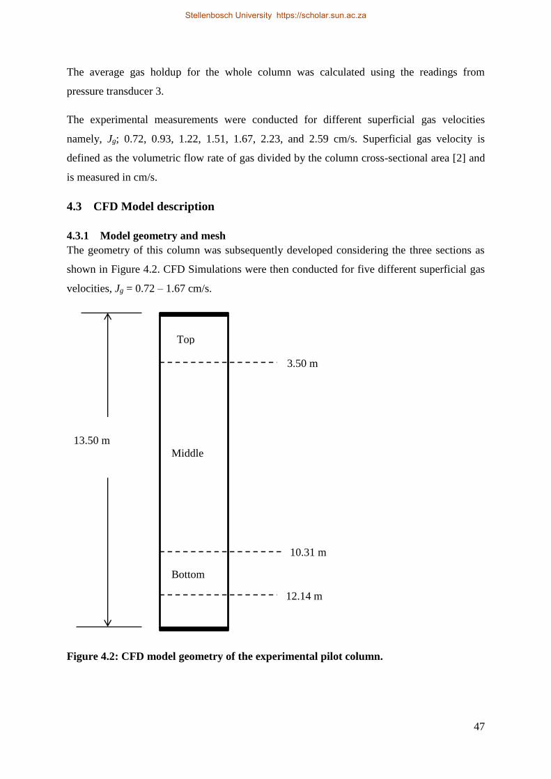
47
The average gas holdup for the whole column was calculated using the readings from
pressure transducer 3.
The experimental measurements were conducted for different superficial gas velocities
namely, Jg; 0.72, 0.93, 1.22, 1.51, 1.67, 2.23, and 2.59 cm/s. Superficial gas velocity is
defined as the volumetric flow rate of gas divided by the column cross-sectional area [2] and
is measured in cm/s.
4.3 CFD Model description
4.3.1 Model geometry and mesh
The geometry of this column was subsequently developed considering the three sections as
shown in Figure 4.2. CFD Simulations were then conducted for five different superficial gas
velocities, Jg = 0.72 – 1.67 cm/s.
Figure 4.2: CFD model geometry of the experimental pilot column.
3.50 m
10.31 m
12.14 m
Middle
Top
Bottom
13.50 m
Stellenbosch University https://scholar.sun.ac.za

48
The meshing application of ANSYS Workbench was used to generate the mesh over the
model geometry. The mesh was generated using the Sweep method which creates a mesh
comprising mainly hexahedral elements. The computational mesh of the column is presented
in Figure 4.3. Grid dependency studies were conducted in order to eliminate the possibility of
errors resulting from an unsuitable mesh size. The mesh was therefore progressively refined
from an initially coarse mesh of cell size equal to 5 cm and number of cells equal to 97188
until there were no significant changes in the simulated axial water and bubble velocity
profiles. The different mesh sizes that were investigated are presented in Table 4.1 while the
axial velocity profiles obtained for these meshes are shown in Figure 4.4 and Figure 4.5. It
can be seen that the mean axial water and bubble velocity profiles do not change significantly
from mesh 3 up to mesh 5. However, the axial velocity for mesh 5 is slightly higher than
mesh 3 and mesh 4. Therefore, based on these results, mesh 4 comprising 884601 elements
with cell size equal to 2.25 cm was used for all subsequent simulations in this study
considering it as a reasonable trade off between the required accuracy and the computational
time of the simulations. A Minimum Orthogonal Quality of 0.840 was obtained for the mesh.
Figure 4.3: CFD mesh for the 0.91 m diameter cylindrical column.
Top view Side view
Stellenbosch University https://scholar.sun.ac.za

49
Table 4.1: Mesh sizes investigated in the grid dependence study.
Identification Element (Cell) Size
in cm
Number of elements Number of nodes
Mesh 1 (coarse mesh) 5.00 97188 106038
Mesh 2 3.75 203280 218764
Mesh 3 2.70 528150 555912
Mesh 4 2.25 884601 925328
Mesh 5 1.85 1611132 1667575
Figure 4.4: Simulated axial water velocity profiles for the investigated mesh sizes
(Superficial gas velocity, Jg = 1.51 cm/s).
-0,2
-0,15
-0,1
-0,05
0
0,05
0,1
0,15
-0,6 -0,4 -0,2 0 0,2 0,4 0,6
Me
an A
xial
Wat
er
Ve
loci
ty (
m/s
)
Radial Position (m)
Mesh 1 Mesh 2 Mesh 3 Mesh 4 Mesh 5
Stellenbosch University https://scholar.sun.ac.za
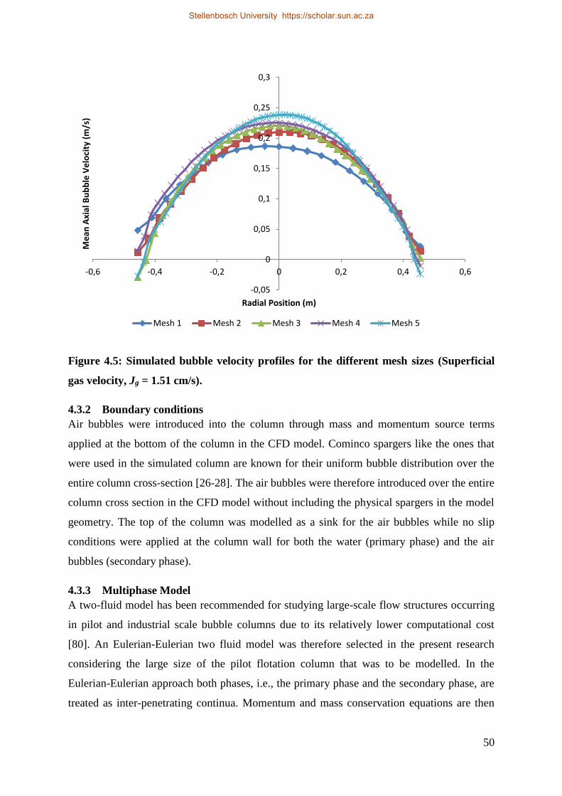
50
Figure 4.5: Simulated bubble velocity profiles for the different mesh sizes (Superficial
gas velocity, Jg = 1.51 cm/s).
4.3.2 Boundary conditions
Air bubbles were introduced into the column through mass and momentum source terms
applied at the bottom of the column in the CFD model. Cominco spargers like the ones that
were used in the simulated column are known for their uniform bubble distribution over the
entire column cross-section [26-28]. The air bubbles were therefore introduced over the entire
column cross section in the CFD model without including the physical spargers in the model
geometry. The top of the column was modelled as a sink for the air bubbles while no slip
conditions were applied at the column wall for both the water (primary phase) and the air
bubbles (secondary phase).
4.3.3 Multiphase Model
A two-fluid model has been recommended for studying large-scale flow structures occurring
in pilot and industrial scale bubble columns due to its relatively lower computational cost
[80]. An Eulerian-Eulerian two fluid model was therefore selected in the present research
considering the large size of the pilot flotation column that was to be modelled. In the
Eulerian-Eulerian approach both phases, i.e., the primary phase and the secondary phase, are
treated as inter-penetrating continua. Momentum and mass conservation equations are then
-0,05
0
0,05
0,1
0,15
0,2
0,25
0,3
-0,6 -0,4 -0,2 0 0,2 0,4 0,6
Me
an A
xial
Bu
bb
le V
elo
city
(m
/s)
Radial Position (m)
Mesh 1 Mesh 2 Mesh 3 Mesh 4 Mesh 5
Stellenbosch University https://scholar.sun.ac.za

51
solved for each of the phases separately. Interaction between the phases was accounted for
through inclusion of the drag force between phases. The Eulerian-Eulerian model has been
reviewed in Chapter 3. The continuity and momentum equations for the Eulerian-Eulerian
model are therefore not repeated here and are given in Chapter 3 as equation (3.3) and
equation (3.4), respectively.
In the present research, water was modelled as the primary phase while air bubbles were
treated as the secondary phase. The volume fraction (or gas holdup) of the secondary phase
was calculated from the mass conservation equations as:
1
𝜌𝑟𝐺(𝜕
𝜕𝑡(휀𝐺𝜌𝐺) + ∇. (휀𝐺𝜌𝐺𝒖𝐺⃗⃗⃗⃗ ⃗) = 𝑆𝐺) (4.2)
where ρrG is the phase reference density, or volume averaged density of the secondary phase
in the solution domain. The volume fraction of the primary phase was calculated from the
secondary phase one, considering that the sum of the volume fractions is equal to 1. In order
to obtain the correct local distribution of the gas phase, previous researchers implemented
compressibility effects in their CFD models using the ideal gas law [22, 32]. Similarly, the
axial gas holdup variation in the present study was accomplished in the CFD simulations by
applying the ideal gas law to compute the density of the secondary phase (ρG) as a function of
the local pressure distribution in the column according to the following equation:
𝜌𝐺 =
𝑝𝑜𝑝 + 𝑝
𝑅𝑀𝑤
𝑇
(4.3)
where p is the local relative (or gauge) pressure predicted by CFD, pop is operating pressure,
R is the universal gas constant, Mw is the molecular weight of the gas, and T is temperature.
4.3.3.1 Drag force formulations
Generally, the drag force per unit volume for bubbles in a swarm is given by [84]:
𝐹 𝐷 =
3휀𝐺휀𝐿
4(𝜌𝐿
𝑑𝐵) 𝐶𝐷|𝒖𝐺⃗⃗⃗⃗ ⃗ − 𝒖𝐿⃗⃗ ⃗⃗ |(𝒖𝐺⃗⃗⃗⃗ ⃗ − 𝒖𝐿⃗⃗ ⃗⃗ ) (4.4)
where CD is the drag coefficient, dB is the bubble diameter, and 𝒖𝐺⃗⃗⃗⃗ ⃗ − 𝒖𝐿⃗⃗ ⃗⃗ is the slip velocity.
The drag force formulation includes the correction for bubble swarms and local volume
fractions of the phases [91]. There are several empirical correlations for the drag coefficient,
CD, in the literature. The drag coefficient is normally presented in these correlations as a
Stellenbosch University https://scholar.sun.ac.za
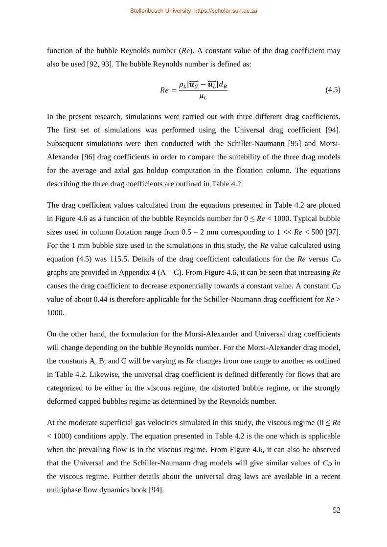
52
function of the bubble Reynolds number (Re). A constant value of the drag coefficient may
also be used [92, 93]. The bubble Reynolds number is defined as:
𝑅𝑒 =
𝜌𝐿|𝒖𝐺⃗⃗⃗⃗ ⃗ − 𝒖𝐿⃗⃗ ⃗⃗ |𝑑𝐵
𝜇𝐿 (4.5)
In the present research, simulations were carried out with three different drag coefficients.
The first set of simulations was performed using the Universal drag coefficient [94].
Subsequent simulations were then conducted with the Schiller-Naumann [95] and Morsi-
Alexander [96] drag coefficients in order to compare the suitability of the three drag models
for the average and axial gas holdup computation in the flotation column. The equations
describing the three drag coefficients are outlined in Table 4.2.
The drag coefficient values calculated from the equations presented in Table 4.2 are plotted
in Figure 4.6 as a function of the bubble Reynolds number for 0 ≤ Re < 1000. Typical bubble
sizes used in column flotation range from 0.5 – 2 mm corresponding to 1 << Re < 500 [97].
For the 1 mm bubble size used in the simulations in this study, the Re value calculated using
equation (4.5) was 115.5. Details of the drag coefficient calculations for the Re versus CD
graphs are provided in Appendix 4 (A – C). From Figure 4.6, it can be seen that increasing Re
causes the drag coefficient to decrease exponentially towards a constant value. A constant CD
value of about 0.44 is therefore applicable for the Schiller-Naumann drag coefficient for Re >
1000.
On the other hand, the formulation for the Morsi-Alexander and Universal drag coefficients
will change depending on the bubble Reynolds number. For the Morsi-Alexander drag model,
the constants A, B, and C will be varying as Re changes from one range to another as outlined
in Table 4.2. Likewise, the universal drag coefficient is defined differently for flows that are
categorized to be either in the viscous regime, the distorted bubble regime, or the strongly
deformed capped bubbles regime as determined by the Reynolds number.
At the moderate superficial gas velocities simulated in this study, the viscous regime (0 ≤ Re
< 1000) conditions apply. The equation presented in Table 4.2 is the one which is applicable
when the prevailing flow is in the viscous regime. From Figure 4.6, it can also be observed
that the Universal and the Schiller-Naumann drag models will give similar values of CD in
the viscous regime. Further details about the universal drag laws are available in a recent
multiphase flow dynamics book [94].
Stellenbosch University https://scholar.sun.ac.za

53
Table 4.2: The drag coefficients that were used in the CFD simulations in the present
study.
Schiller and
Naumann[95] 𝐶𝐷 = {
24
𝑅𝑒[1 + 0.15𝑅𝑒0.687] 𝑓𝑜𝑟 𝑅𝑒 < 1000
0.44 𝑓𝑜𝑟 𝑅𝑒 > 1000 (4.6)
Morsi and
Alexander[96] 𝐶𝐷 =
𝐴
𝑅𝑒+
𝐵
𝑅𝑒2+ 𝐶
𝐴 𝐵 𝐶𝑅𝑒 < 0.1 24 0 00.1 ≤ 𝑅𝑒 < 1 22.73 0.0903 3.691 ≤ 𝑅𝑒 < 10 29.1667 −3.8889 1.22210 ≤ 𝑅𝑒 < 100 46.5 −116.67 0.6167100 ≤ 𝑅𝑒 < 1000 98.33 −2778 0.36441000 ≤ 𝑅𝑒 < 5000 148.62 −4.75 × 10⁴ 0.3575000 ≤ 𝑅𝑒 < 10000 −490.546 5.787 × 10⁵ 0.4610000 ≤ 𝑅𝑒 < 50000 −1662.5 5.4167 × 10⁶ 0.5191𝑅𝑒 ≥ 50000 0 0 0.44
(4.7)
Universal
drag[94] 𝐶𝐷𝑣𝑖𝑠
=24
𝑅𝑒(1 + 0.1𝑅𝑒0.75)
where Re is the relative Reynolds number for the primary phase L
and the secondary phase G obtained on the basis of the relative
velocity of the two phases as:-
𝑅𝑒 =𝜌𝐿|𝒖𝐿⃗⃗ ⃗⃗ − 𝒖𝐺⃗⃗⃗⃗ ⃗|𝑑𝐵
𝜇𝑒
where μe is the effective viscosity of the primary phase considering
the effects of the secondary phase.
𝜇𝑒 =𝜇𝐿
1 − 휀𝐺
(4.8)
Stellenbosch University https://scholar.sun.ac.za

54
Figure 4.6: Drag coefficient CD as a function of bubble Reynolds number Re for 0 ≤ Re <
1000.
4.3.4 Turbulence model
Turbulence was modelled using the realizable k-ϵ turbulence model which is a RANS
(Reynolds- Averaged Navier-Stokes) based model. In the RANS modelling approach, the
instantaneous Navier-Stokes equations are replaced with the time averaged Navier-Stokes
(RANS) equations which are solved to produce a time averaged flow field. The averaging
procedure introduces additional unknowns, the Reynolds stresses. The Reynolds stresses are
subsequently resolved by employing Boussinesq’s eddy viscosity concept where the
Reynolds stresses (or turbulent stresses) are related to the velocity gradients according
equation (3.9). The eddy (turbulent) viscosity is then modelled as outlined in equation (3.13)
and equation (3.14).
4.3.5 Numerical solution methods
Momentum and volume fraction equations were discretized using the QUICK scheme, while
First Order Upwind was employed for turbulence kinetic energy and dissipation rate
0
0,2
0,4
0,6
0,8
1
1,2
1,4
1,6
1,8
0 200 400 600 800 1000
Dra
g co
effi
cien
t, C
D
Bubble Reynolds number, Re
CD as a function of Re
Schiller Naumann Morsi Alexander Universal drag
Stellenbosch University https://scholar.sun.ac.za

55
discretization. The QUICK scheme provides up to third-order accuracy in the computations,
while First Order Upwind is easier to converge. The time step size was 0.05s.
For simulations that were difficult to converge the First Order Upwind scheme was used in
place of the QUICK scheme until convergence. In some of such cases the time step size was
changed from 0.05s to 0.025s to enhance convergence. The simulations were run up to flow
times of between 400s and 540s since the bubble residence time in a similar sized column
was measured to be between 4-5 minutes [98].
4.4 Results and discussion
Two sets of CFD simulations were carried out in this study to predict the average gas holdup
and the axial gas holdup variation in the flotation column. The first set of simulations was
conducted using the Universal drag coefficient to calculate the drag force between the air
bubbles and the liquid. Another set of simulations was then performed with the Schiller-
Naumann and the Morsi-Alexander drag coefficients in order to compare the suitability of the
different drag models for predicting gas holdup in the column. The physical parameters used
in the simulations are defined in Table 4.3: Parameters used in the CFD simulations.. The
simulation results obtained with the Universal drag are presented first followed by a
comparison of the results obtained with the three different drag coefficients.
Table 4.3: Parameters used in the CFD simulations.
Liquid phase (water)
Density 998.2 kg/m3
Viscosity 0.001 kg/m-s
Gas phase (air bubbles)
Density 1.225 kg/m3; for compressible flow, density
was calculated using the Ideal Gas law
Viscosity 1.789 x 10⁻⁵ kg/m-s
Bubble diameter 1 mm
4.4.1 Simulation results with Universal drag coefficient
4.4.1.1 Liquid flow field
The predicted velocity vectors of the liquid (water) in the column are shown in Figure 4.7.
The liquid velocity field shows a typical circulating flow in the column in which the liquid is
rising in the centre and descending near the walls of the column. This compares well with
Stellenbosch University https://scholar.sun.ac.za

56
earlier CFD predictions for flotation columns [11, 13] as well as experimental data on bubble
columns [48, 50].
The type of liquid circulation where upward flow exists in the centre while downward flow
prevails near the column walls is referred to as gulf-stream circulation [49]. This liquid
circulation pattern has been attributed to density differences arising from non-uniform radial
gas holdup profiles [48, 49].
The simulated axial velocity profile of water at the mid-height position in the column is
presented in Figure 4.8. It can be seen in this Figure that the water velocity is positive
(upward) in the centre of the column and negative (downward) near the wall hence
confirming the gulf-stream circulation pattern in the column. The axial water velocity profile
shown in Figure 4.8 is asymmetrical. Asymmetrical velocity profiles have also been reported
by other researchers who conducted experimental studies on bubble columns [50].
Figure 4.7: Vectors showing the predicted flow of water in the column (superficial gas
velocity, Jg = 0.93 cm/s).
Bottom part Middle part Top part
Stellenbosch University https://scholar.sun.ac.za
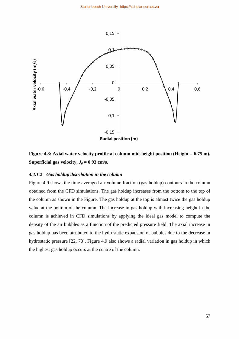
57
Figure 4.8: Axial water velocity profile at column mid-height position (Height = 6.75 m).
Superficial gas velocity, Jg = 0.93 cm/s.
4.4.1.2 Gas holdup distribution in the column
Figure 4.9 shows the time averaged air volume fraction (gas holdup) contours in the column
obtained from the CFD simulations. The gas holdup increases from the bottom to the top of
the column as shown in the Figure. The gas holdup at the top is almost twice the gas holdup
value at the bottom of the column. The increase in gas holdup with increasing height in the
column is achieved in CFD simulations by applying the ideal gas model to compute the
density of the air bubbles as a function of the predicted pressure field. The axial increase in
gas holdup has been attributed to the hydrostatic expansion of bubbles due to the decrease in
hydrostatic pressure [22, 73]. Figure 4.9 also shows a radial variation in gas holdup in which
the highest gas holdup occurs at the centre of the column.
-0,15
-0,1
-0,05
0
0,05
0,1
0,15
-0,6 -0,4 -0,2 0 0,2 0,4 0,6
Axi
al w
ater
vel
oci
ty (
m/s
)
Radial position (m)
Stellenbosch University https://scholar.sun.ac.za

58
Figure 4.9: Gas holdup contours – time averaged air volume fraction (Jg = 0.93 cm/s).
The CFD model was further tested for the case in which the effect of the hydrostatic pressure
is neglected. In this case, the air bubbles were assigned a constant density of 1.225 kg/m3. In
other words, simulation results in which the air bubbles were modelled as incompressible
(without hydrostatic ‘expansion’) were compared with the results in which compressibility
effects are accounted for using the ideal gas law. This was done in order to determine
whether there was no other source of change in axial gas holdup. The axial gas holdup
profiles of the two cases are compared in Figure 4.10. The case with compressibility effects
shows an axial gas holdup profile in which the gas holdup increases by at least 100% from
bottom to top along the height of the column. On the other hand, the incompressible case
does not show significant increase in axial gas holdup. The decreasing hydrostatic pressure
therefore plays the major role in creating an axial gas holdup profile in flotation columns.
Stellenbosch University https://scholar.sun.ac.za

59
Figure 4.10: Comparison of CFD simulations with hydrostatic pressure effects
(compressibility) and the case without hydrostatic bubble 'expansion' (incompressible);
Jg = 1.51 cm/s.
4.4.1.3 Comparison of predicted gas holdup with experimental data
The gas holdup was obtained from CFD simulations as a volume-weighted average volume
fraction of the air bubbles. The predicted average gas holdup is the net volume-weighted
average volume fraction for the three sections (bottom, middle, and top) of the column while
axial gas holdup was determined from the local value of air volume fraction in each of the
three sections. Figure 4.11 is the parity plot comparing the simulated (predicted) average gas
holdup against the experimental gas holdup measurements [18]. The CFD predictions seem to
be in good agreement with the experimental data since all the points lie close to the line y = x
as shown in the Figure.
0
2
4
6
8
10
12
14
0,02 0,04 0,06 0,08 0,1 0,12 0,14
He
igh
t (m
)
Gas holdup (time averaged)
With compressibility Without compressibility
Stellenbosch University https://scholar.sun.ac.za

60
Figure 4.11: Parity plot comparing the predicted (CFD) average gas holdup and the
experimental data [18].
The axial gas holdup predicted for each of the three sections (bottom, middle, and top) of the
column is also compared against experimental data in Figure 4.12 – Figure 4.15. The increase
of gas holdup along the column height can be observed both in the CFD predictions and
experimental data as shown in these Figures.
The axial gas holdup prediction for the middle part of the column gave an excellent
comparison with experimental data while the top part was slightly under-predicted for the
higher superficial gas velocities (Jg = 1.51 cm/s and 1.67 cm/s). On the other hand, it can be
observed from Figure 4.12 – Figure 4.15 that the axial gas holdup is over-predicted for the
bottom part of the column especially at lower superficial gas velocities (Jg = 0.72 and 0.93
cm/s). This is because the CFD model applies a constant bubble size of 1 mm and does not
account for bubble coalescence and break up in the column. At lower superficial gas
velocities bubble coalescence will be the dominant process compared to bubble break up
[99], hence the experimental gas holdup in the bottom part of the column will be lower than
the predicted one. However, with increasing Superficial gas velocity bubble break up
probably reduces the average bubble size to around the 1 mm value used in the simulations,
0
1
2
3
4
5
6
7
8
9
10
0 2 4 6 8 10
Pre
dic
ted
gas
ho
ldu
p (
%)
Experimental gas holdup (%)
Stellenbosch University https://scholar.sun.ac.za
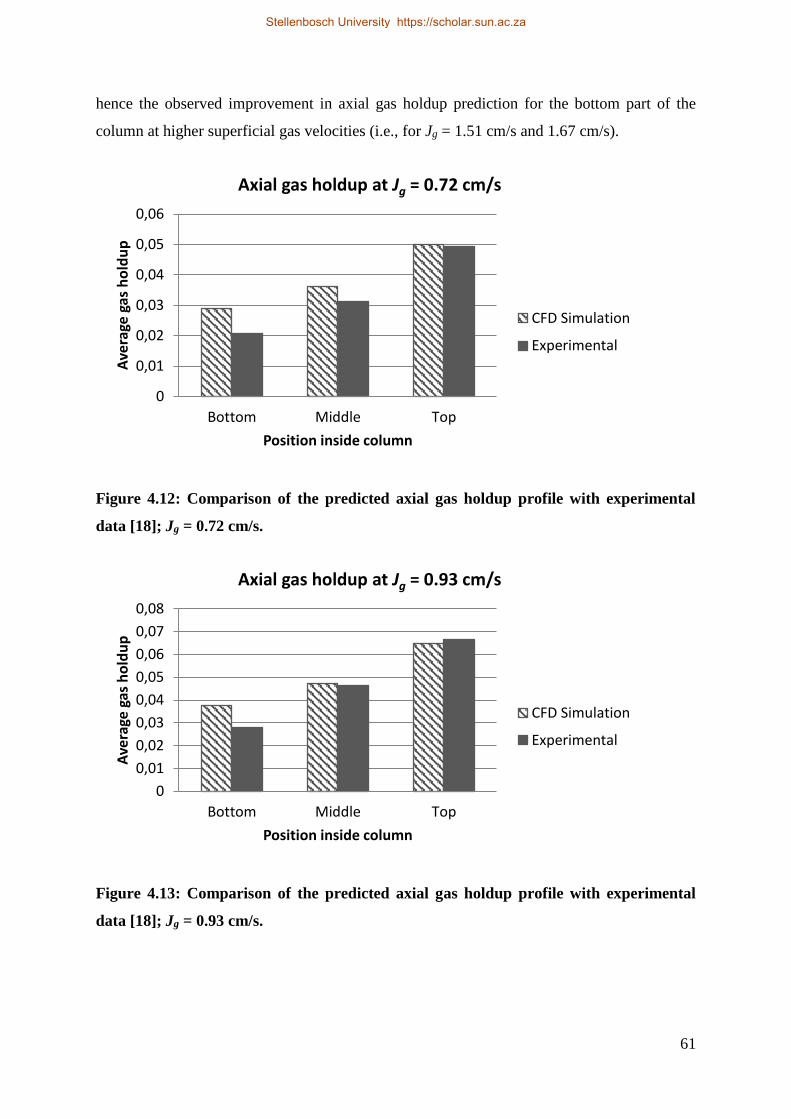
61
hence the observed improvement in axial gas holdup prediction for the bottom part of the
column at higher superficial gas velocities (i.e., for Jg = 1.51 cm/s and 1.67 cm/s).
Figure 4.12: Comparison of the predicted axial gas holdup profile with experimental
data [18]; Jg = 0.72 cm/s.
Figure 4.13: Comparison of the predicted axial gas holdup profile with experimental
data [18]; Jg = 0.93 cm/s.
0
0,01
0,02
0,03
0,04
0,05
0,06
Bottom Middle Top
Ave
rage
gas
ho
ldu
p
Position inside column
Axial gas holdup at Jg = 0.72 cm/s
CFD Simulation
Experimental
0
0,01
0,02
0,03
0,04
0,05
0,06
0,07
0,08
Bottom Middle Top
Ave
rage
gas
ho
ldu
p
Position inside column
Axial gas holdup at Jg = 0.93 cm/s
CFD Simulation
Experimental
Stellenbosch University https://scholar.sun.ac.za

62
Figure 4.14: Comparison of the predicted axial gas holdup profile with experimental
data [18]; Jg = 1.51 cm/s.
Figure 4.15: Comparison of the predicted axial gas holdup profile with experimental
data [18]; Jg = 1.67 cm/s.
4.4.1.4 Bubble velocities
Table 4.4 shows the volume weighted average velocity magnitude of air bubbles obtained
from the CFD simulations at different superficial gas velocities. For the constant bubble size
of 1 mm used in the CFD simulations, the average velocity magnitude seems to decrease
0
0,02
0,04
0,06
0,08
0,1
0,12
Bottom Middle Top
Ave
rage
gas
ho
ldu
p
Position inside column
Axial gas holdup at Jg = 1.51 cm/s
CFD Simulation
Experimental
0
0,02
0,04
0,06
0,08
0,1
0,12
0,14
Bottom Middle Top
Ave
rage
gas
ho
ldu
p
Position inside column
Axial gas holdup at Jg = 1.67 cm/s
CFD Simulation
Experimental
Stellenbosch University https://scholar.sun.ac.za

63
slightly with increasing superficial gas velocity. This is perhaps due to the increase in average
gas holdup resulting from increasing the superficial gas velocity [100-102].
Table 4.4: Predicted average velocities of air bubbles at different superficial gas
velocities.
Superficial gas velocity (cm/s) Average Velocity Magnitude of air
bubbles (cm/s)
0.72 12.79
0.93 12.33
1.22 11.78
1.51 11.84
1.67 11.61
The simulated axial velocity profiles of air bubbles at different heights in the column are
shown in Figure 4.16 for Jg = 1.51 cm/s. It can be seen that the axial bubble velocity
decreases with height along the column. Previous research on axial velocity profiles of single
bubbles also identified similar bubble behaviour along the column height due to the
progressive increase in the drag coefficient resulting from surfactant-induced changes at the
bubble surface [31]. However, since the effects of surfactants on bubble surfaces are not
accounted for in the present CFD model, the observed axial variation in bubble velocity in
this case must have its origins in some other mechanism, possibly the increase in the drag
force resulting from the increase in gas holdup with height along the column. The observed
decrease in bubble velocity with column height could result in a further increase in axial gas
holdup variations. Figure 4.16 also also shows a change in the shape of the axial bubble
velocity profile from a parabolic shape at the bottom and in the middle to a more uniform
profile at the top of the column where the flow turbulence is fully developed.
In Figure 4.17, the axial velocity of bubbles is plotted against height along the column axis.
The profile obtained shows three stages of the velocity profile similar to the three-stage
profile described by Sam et al. [31] for single bubbles rising in a 4 m water column in the
presence of frother. In the initial stage, the bubble velocity increases rapidly (acceleration
stage) to reach a maximum velocity of 23.2 cm/s at height approximately 2.7 m in the
column. This value compares favourably with the maximum velocity of 25.0±0.4 cm/s
reported by Sam et al. [31] for bubbles of 0.9 mm diameter. In the second stage (deceleration
Stellenbosch University https://scholar.sun.ac.za

64
stage), the bubble velocity is decreasing until at height approximately 8.5 m. After that the
bubble velocity appears to fluctuate around an average velocity of about 11.5 cm/s (constant
velocity or terminal velocity stage). This value can be compared to the terminal velocities of
between 11.0 and 12.0 cm/s observed by Sam et al. [31] for similar bubble size (0.9 mm
bubble diameter).
An interesting observation here is that in spite of the fact that our CFD model does not
account for the effects of frother, the results in Figure 4.17 are quiet similar to the three-stage
profile described by Sam et al. [31] for bubbles rising in water in the presence of frother
where the decreasing velocity in stage 2 was attributed to progressive adsorption of surfactant
molecules as the bubble rises. On the other hand, equation (4.4) indicates that the drag force
on the air bubbles should increase with increasing volume fraction of the bubbles (or gas
holdup). The deceleration of bubbles observed in the CFD results could therefore be related
to the increase in gas holdup along the column axis due to subsequent increases in the drag
force.
Figure 4.16: Axial velocity profiles of air bubbles at three different heights along the
column; Jg = 1.51 cm/s.
-0,05
0
0,05
0,1
0,15
0,2
0,25
-0,6 -0,4 -0,2 0 0,2 0,4 0,6
Axi
al B
ub
ble
Ve
loci
ty (
m/s
)
Radial position (m)
Position 10 m height Position 6.75 m height Position 3.50 m height
Stellenbosch University https://scholar.sun.ac.za
65
Figure 4.17: Axial bubble velocity versus height along the column axis; Jg = 1.51 cm/s.
4.4.2 Comparison of average and axial gas holdup predicted using different drag
coefficients
In this research, simulations were also performed to compare the gas holdup prediction when
different drag coefficient formulations were used. In this regard, CFD simulations were
carried out with three drag models, the Universal drag, Schiller and Naumann, and the Morsi
and Alexander models. The parity plot comparing the average gas holdup prediction for the
different drag coefficients is shown in Figure 4.18. It can be seen that there is no significant
difference between the results obtained with the three drag coefficients.
0
2
4
6
8
10
12
14
0 0,05 0,1 0,15 0,2 0,25
He
igh
t (m
)
Axial Bubble Velocity (m/s)
Stellenbosch University https://scholar.sun.ac.za
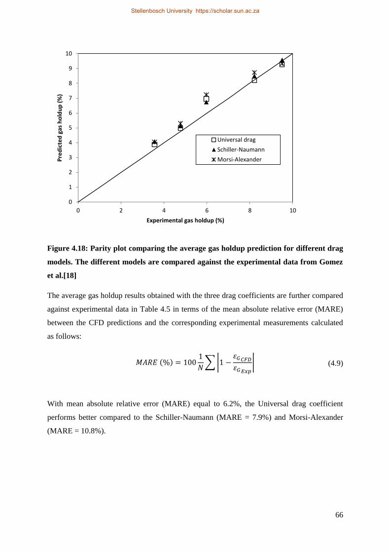
66
Figure 4.18: Parity plot comparing the average gas holdup prediction for different drag
models. The different models are compared against the experimental data from Gomez
et al.[18]
The average gas holdup results obtained with the three drag coefficients are further compared
against experimental data in Table 4.5 in terms of the mean absolute relative error (MARE)
between the CFD predictions and the corresponding experimental measurements calculated
as follows:
𝑀𝐴𝑅𝐸 (%) = 100
1
𝑁∑|1 −
휀𝐺𝐶𝐹𝐷
휀𝐺𝐸𝑥𝑝
| (4.9)
With mean absolute relative error (MARE) equal to 6.2%, the Universal drag coefficient
performs better compared to the Schiller-Naumann (MARE = 7.9%) and Morsi-Alexander
(MARE = 10.8%).
0
1
2
3
4
5
6
7
8
9
10
0 2 4 6 8 10
Pre
dic
ted
gas
ho
ldu
p (
%)
Experimental gas holdup (%)
Universal drag
Schiller-Naumann
Morsi-Alexander
Stellenbosch University https://scholar.sun.ac.za

67
Table 4.5: Comparison of average gas holdup predicted using different drag
coefficients.
UNIVERSAL DRAG
Superficial gas velocity
(cm/s)
Average gas holdup (%) -
Experimental
Gas Holdup
(%) - CFD
Relative
Error
0.72 3.56 3.86 0.084
0.93 4.77 4.98 0.044
1.22 5.97 6.91 0.157
1.51 8.21 8.20 0.001
1.67 9.50 9.27 0.024
Mean absolute relative error (MARE) = 6.22%
SCHILLER NAUMANN
Superficial gas velocity
(cm/s)
Average gas holdup (%) -
Experimental
Gas Holdup
(%) - CFD
Relative
Error
0.72 3.56 4.08 0.146
0.93 4.77 5.13 0.075
1.22 5.97 6.74 0.129
1.51 8.21 8.50 0.035
1.67 9.50 9.58 0.008
Mean absolute relative error (MARE) = 7.89%
MORSI ALEXANDER
Superficial gas velocity
(cm/s)
Average gas holdup (%) -
Experimental
Gas Holdup
(%) - CFD
Relative
Error
0.72 3.56 4.05 0.138
0.93 4.77 5.29 0.109
1.22 5.97 7.22 0.209
1.51 8.21 8.74 0.065
1.67 9.50 9.33 0.018
Mean absolute relative error (MARE) = 10.77%
Stellenbosch University https://scholar.sun.ac.za

68
The Axial gas holdup predictions using the different drag coefficients are compared with
experimental data [18] in Figure 4.19– Figure 4.22. There is again no significant difference
between the results obtained with the three drag coefficients. For all the three drag models, the
gas hold up prediction was very good for the middle part of the column, good for the top part,
and over predicted at low superficial gas velocity (Jg = 0.72 cm/s and 0.93 cm/s) for the bottom
part of the column. The over-prediction of the local gas holdup at the bottom part of the column
can be attributed to bubble coalescence as already explained above. The mean absolute relative
error calculated for the different drag coefficients for the axial gas holdup prediction are
presented in Table 4.6 – Table 4.8. Mean absolute relative error above 20% was obtained for the
gas holdup prediction in the bottom part of the column with all three drag coefficients. On the
other hand, the gas holdup in the middle and top parts of the column was predicted with less than
10% relative error.
Figure 4.19: Comparison of axial gas holdup prediction for different drag coefficients;
superficial gas velocity, Jg = 0.72 cm/s.
0
1
2
3
4
5
6
Bottom Middle Top
Gas
ho
ldu
p (
%)
Position inside column
Axial gas holdup at Jg = 0.72 cm/s
Universal drag
Schiller-Naumann
Morsi-Alexander
Experimental
Stellenbosch University https://scholar.sun.ac.za
Stellenbosch University https://scholar.sun.ac.za

69
Figure 4.20: Comparison of axial gas holdup prediction for different drag coefficients;
superficial gas velocity, Jg = 0.93 cm/s.
Figure 4.21: Comparison of gas holdup prediction for different drag coefficients; superficial
gas velocity, Jg = 1.51 cm/s.
0
1
2
3
4
5
6
7
8
Bottom Middle Top
Gas
ho
ldu
p (
%)
Position inside column
Axial gas holdup at Jg = 0.93 cm/s
Universal drag
Schiller-Naumann
Morsi-Alexander
Experimental
0
2
4
6
8
10
12
Bottom Middle Top
Gas
ho
ldu
p (
%)
Position inside column
Axial gas holdup at Jg = 1.51 cm/s
Universal drag
Schiller-Naumann
Morsi-Alexander
Experimental
Stellenbosch University https://scholar.sun.ac.za
Stellenbosch University https://scholar.sun.ac.za

70
Figure 4.22: Comparison of gas holdup prediction for different drag coefficients; superficial
gas velocity, Jg = 1.67 cm/s.
0
2
4
6
8
10
12
14
Bottom Middle Top
Gas
ho
ldu
p (
%)
Position inside column
Axial gas holdup at Jg = 1.67 cm/s
Universal drag
Schiller-Naumann
Morsi-Alexander
Experimental
Stellenbosch University https://scholar.sun.ac.za
Stellenbosch University https://scholar.sun.ac.za
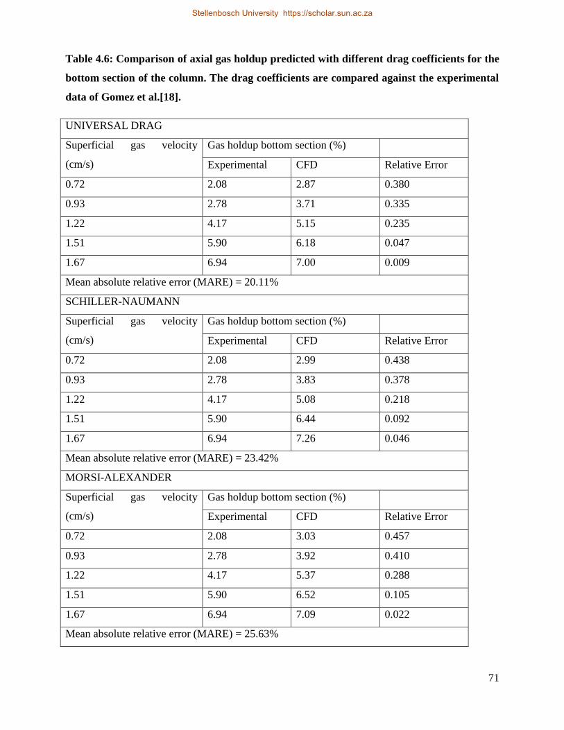
71
Table 4.6: Comparison of axial gas holdup predicted with different drag coefficients for the
bottom section of the column. The drag coefficients are compared against the experimental
data of Gomez et al.[18].
UNIVERSAL DRAG
Superficial gas velocity
(cm/s)
Gas holdup bottom section (%)
Experimental CFD Relative Error
0.72 2.08 2.87 0.380
0.93 2.78 3.71 0.335
1.22 4.17 5.15 0.235
1.51 5.90 6.18 0.047
1.67 6.94 7.00 0.009
Mean absolute relative error (MARE) = 20.11%
SCHILLER-NAUMANN
Superficial gas velocity
(cm/s)
Gas holdup bottom section (%)
Experimental CFD Relative Error
0.72 2.08 2.99 0.438
0.93 2.78 3.83 0.378
1.22 4.17 5.08 0.218
1.51 5.90 6.44 0.092
1.67 6.94 7.26 0.046
Mean absolute relative error (MARE) = 23.42%
MORSI-ALEXANDER
Superficial gas velocity
(cm/s)
Gas holdup bottom section (%)
Experimental CFD Relative Error
0.72 2.08 3.03 0.457
0.93 2.78 3.92 0.410
1.22 4.17 5.37 0.288
1.51 5.90 6.52 0.105
1.67 6.94 7.09 0.022
Mean absolute relative error (MARE) = 25.63%
Stellenbosch University https://scholar.sun.ac.za
Stellenbosch University https://scholar.sun.ac.za

72
Table 4.7: Comparison of axial gas holdup predicted with different drag coefficients for the
middle section of the column. The drag coefficients are compared against the experimental
data of Gomez et al.[18].
UNIVERSAL DRAG
Superficial gas velocity
(cm/s)
Gas holdup middle section (%)
Experimental CFD Relative Error
0.72 3.11 3.57 0.148
0.93 4.64 4.61 0.006
1.22 5.84 6.44 0.103
1.51 7.79 7.67 0.015
1.67 8.72 8.66 0.007
Mean absolute relative error (MARE) = 5.59%
SCHILLER-NAUMANN
Superficial gas velocity
(cm/s)
Gas holdup middle section (%)
Experimental CFD Relative Error
0.72 3.11 3.77 0.212
0.93 4.64 4.78 0.030
1.22 5.84 6.29 0.077
1.51 7.79 7.94 0.019
1.67 8.72 8.96 0.028
Mean absolute relative error (MARE) = 7.32%
MORSI-ALEXANDER
Superficial gas velocity
(cm/s)
Gas holdup middle section (%)
Experimental CFD Relative Error
0.72 3.11 3.73 0.199
0.93 4.64 4.90 0.056
1.22 5.84 6.70 0.147
1.51 7.79 8.16 0.047
1.67 8.72 8.75 0.003
Mean absolute relative error (MARE) = 9.072%
Stellenbosch University https://scholar.sun.ac.za
Stellenbosch University https://scholar.sun.ac.za
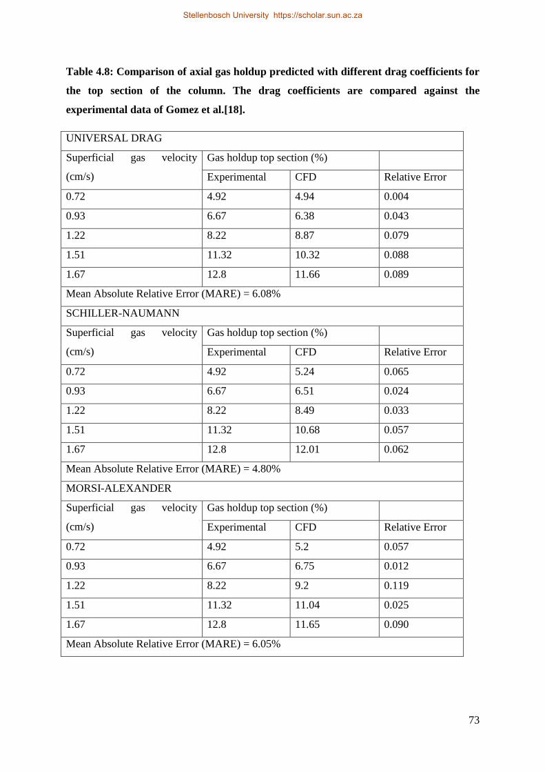
73
Table 4.8: Comparison of axial gas holdup predicted with different drag coefficients for
the top section of the column. The drag coefficients are compared against the
experimental data of Gomez et al.[18].
UNIVERSAL DRAG
Superficial gas velocity
(cm/s)
Gas holdup top section (%)
Experimental CFD Relative Error
0.72 4.92 4.94 0.004
0.93 6.67 6.38 0.043
1.22 8.22 8.87 0.079
1.51 11.32 10.32 0.088
1.67 12.8 11.66 0.089
Mean Absolute Relative Error (MARE) = 6.08%
SCHILLER-NAUMANN
Superficial gas velocity
(cm/s)
Gas holdup top section (%)
Experimental CFD Relative Error
0.72 4.92 5.24 0.065
0.93 6.67 6.51 0.024
1.22 8.22 8.49 0.033
1.51 11.32 10.68 0.057
1.67 12.8 12.01 0.062
Mean Absolute Relative Error (MARE) = 4.80%
MORSI-ALEXANDER
Superficial gas velocity
(cm/s)
Gas holdup top section (%)
Experimental CFD Relative Error
0.72 4.92 5.2 0.057
0.93 6.67 6.75 0.012
1.22 8.22 9.2 0.119
1.51 11.32 11.04 0.025
1.67 12.8 11.65 0.090
Mean Absolute Relative Error (MARE) = 6.05%
Stellenbosch University https://scholar.sun.ac.za

74
4.5 Conclusions
CFD modelling was applied to study the gas holdup and its variation along the collection
zone of a pilot flotation column. Both the predicted average gas holdup and the axial (local)
gas holdup were in good agreement with the experimental data available in the literature. The
generally known gas distribution profile, with the gas holdup increasing upward in the
column and having maximum values in the column centre was also predicted by the CFD
simulations.
Three drag models, the Universal drag, Schiller-Naumann, and Morsi-Alexander drag
coefficients were compared in this study in order to determine the suitable drag model for
average and axial gas holdup prediction in the column. The three drag coefficients all
produced good prediction of both the average and local gas holdup. Therefore, any of these
three drag coefficients can be used to model flotation column hydrodynamics.
An axial velocity profile was also observed in which the bubble velocity magnitude
decreased with height along the column. The reason for this could be the increase in drag
force resulting from the axial increase in gas holdup along the column height. However, the
decrease in axial bubble velocity along the column height can result in a further increase in
the axial gas holdup variations compared to the effect of the hydrostatic pressure only. The
axial variation in gas holdup could therefore be explained as having its origins in two inter-
related processes – the hydrostatic expansion of air bubbles and the development of a bubble
velocity profile in which the axial velocity of bubbles decreases with height along the
column.
Stellenbosch University https://scholar.sun.ac.za

75
Chapter 5 CFD Simulation of the mixing characteristics of industrial
flotation columns
5.1 Introduction
In this chapter, the mixing characteristics of the collection zone of industrial flotation
columns are investigated using Computational Fluid Dynamics (CFD). Flotation columns are
known for their improved metallurgical performance compared to conventional flotation
cells. However, increased mixing in the column can adversely affect its grade/recovery
performance.
It has been observed that mineral recovery decreases as the mixing conditions increase from
plug flow towards perfectly mixed flow in the column [2, 56]. A high degree of mixing will
therefore have detrimental effects on the overall performance of a flotation column. As a
result, the design and optimization of flotation columns require detailed knowledge of the
effects of various geometrical and operational parameters on the mixing characteristics of the
column.
The mixing characteristics of flotation columns have been studied by several researchers [58,
64, 65, 103, 104]. However, there are still uncertainties particularly with regard to solids
mixing characteristics in the column. The earlier studies by Dobby and Finch [58] and
Yianatos and Bergh [65] suggested that the solids and liquid axial dispersion coefficients
were equal. On the other hand, several authors have questioned the equivalence of the solids
and liquid dispersion citing various reasons [61, 105, 106]. Some researchers have also
investigated the effect of solids on the liquid dispersion in the column [40, 59]. It has been
reported that the liquid dispersion decreased as the percentage of solids in the feed increased,
possibly due to viscous effects. However, the effect of particle size on the liquid dispersion
has not yet been studied.
The studies described above were entirely based on experimental methods which did not
provide detailed information of the solids and liquid flow patterns inside the flotation column.
On the other hand, Computational Fluid Dynamics (CFD) is an alternative modelling tool
which is based on the flow physics of the process. CFD methodology can therefore be used in
the study of the mixing characteristics of flotation columns, with the additional advantage of
basing the interpretation of the results on the flow patterns derived from numerical
simulations. Despite the fact that CFD can potentially be useful in the design and
Stellenbosch University https://scholar.sun.ac.za
76
optimization of column flotation, there seems to be a limited amount of literature on the
subject. In addition, the few column flotation CFD models in the literature in which mixing is
investigated have simulated two phase (gas-liquid) flows only while solids have not been
included in the column [11, 15].
Deng et al. [11] applied numerical simulations to study the flows in flotation columns. They
predicted a liquid circulation pattern in which the axial liquid velocity was upward in the
centre and downward near the walls of the column. The mixing in the flotation column was
further attributed to the liquid circulation pattern established in the column. However, the
actual mixing was not simulated in terms of residence time distributions (RTDs).
Subsequent studies were conducted by Xia et al. [15] who used a two-dimensional CFD
model to simulate the alleviation of liquid back-mixing by baffles and packings in a flotation
column. Their study revealed that the liquid back-mixing in an open bubble/flotation column
could be alleviated using baffles and packings. However, the liquid RTD simulations were
not conducted in order to quantify the actual mixing parameters in the open column compared
to the baffled column and the column with packings.
The aim of the study presented in this chapter was, therefore, to investigate the mixing
characteristics of industrial flotation columns using Computational Fluid Dynamics (CFD). In
this regard, CFD models were developed for the 0.45 m square column and the 0.91 m
diameter cylindrical column from the work of Dobby and Finch [58] and Yianatos and Bergh
[65], respectively. These authors’ data was therefore used to validate the present modelling
approach. Specifically, the work presented in this chapter involves numerical simulations of
residence time distributions (RTDs) of both the liquid and solid phases in industrial columns.
The simulated RTDs are then used to determine the mixing parameters, i.e., the mean
residence time and the vessel dispersion number. Both the mean residence time and the vessel
dispersion number are useful parameters in the design and scale-up equations for column
flotation.
In addition, the simulated flow patterns of the solid and liquid phases are compared in order
to understand the relationship between the solid and liquid dispersion characteristics. The
effects of particle size and bubble size on liquid back-mixing in the column are also
investigated.
Stellenbosch University https://scholar.sun.ac.za

77
5.2 Theory
The one-dimensional (axial) plug flow dispersion model is applicable to describe the axial
mixing process in the collection zone of the flotation column [2]. In this case, the degree of
mixing is quantified by the axial dispersion coefficient D (units of length2/time) or the
dimensionless vessel dispersion (Nd).
Two extreme cases of mixing exist, namely:
Plug flow (negligible dispersion), Nd → 0
Perfectly mixed reactor (large dispersion), Nd → ∞
The vessel dispersion number is given by:
𝑁𝑑 =
𝐷
𝑢𝐻 (5.1)
where u is either the liquid interstitial velocity or the particle velocity and H is the height of
the collection zone.
The axial dispersion coefficient (D) or the vessel dispersion number (Nd) can be calculated
from Residence Time Distribution (RTD) data using two parameters: the mean residence time
(τ) and the variance or measure of the spread of the RTD curve (σ2). These measures are
directly related by theory to D and/or Nd. In this study, the mean residence time was
calculated from the first moment about the origin according to the following equation [107]:
𝜏 =
∫ 𝑡 𝐶 𝑑𝑡∞
0
∫ 𝐶 𝑑𝑡∞
0
=∑𝑡𝐶∆𝑡
∑𝐶∆𝑡 (5.2)
On the other hand, the variance is given by the second moment about the mean as follows:
𝜎2 =
∫ (𝑡 − 𝜏)2 𝐶 𝑑𝑡∞
0
∫ 𝐶 𝑑𝑡∞
0
=∫ 𝑡2 𝐶 𝑑𝑡
∞
0
∫ 𝐶 𝑑𝑡∞
0
− 𝜏2 (5.3)
For a set of discrete data points, the variance is expressed as:
𝜎2 ≅
∑(𝑡 − 𝜏)2𝐶∆𝑡
∑𝐶∆𝑡=
∑ 𝑡2𝐶∆𝑡
∑𝐶∆𝑡− 𝜏2 (5.4)
Stellenbosch University https://scholar.sun.ac.za
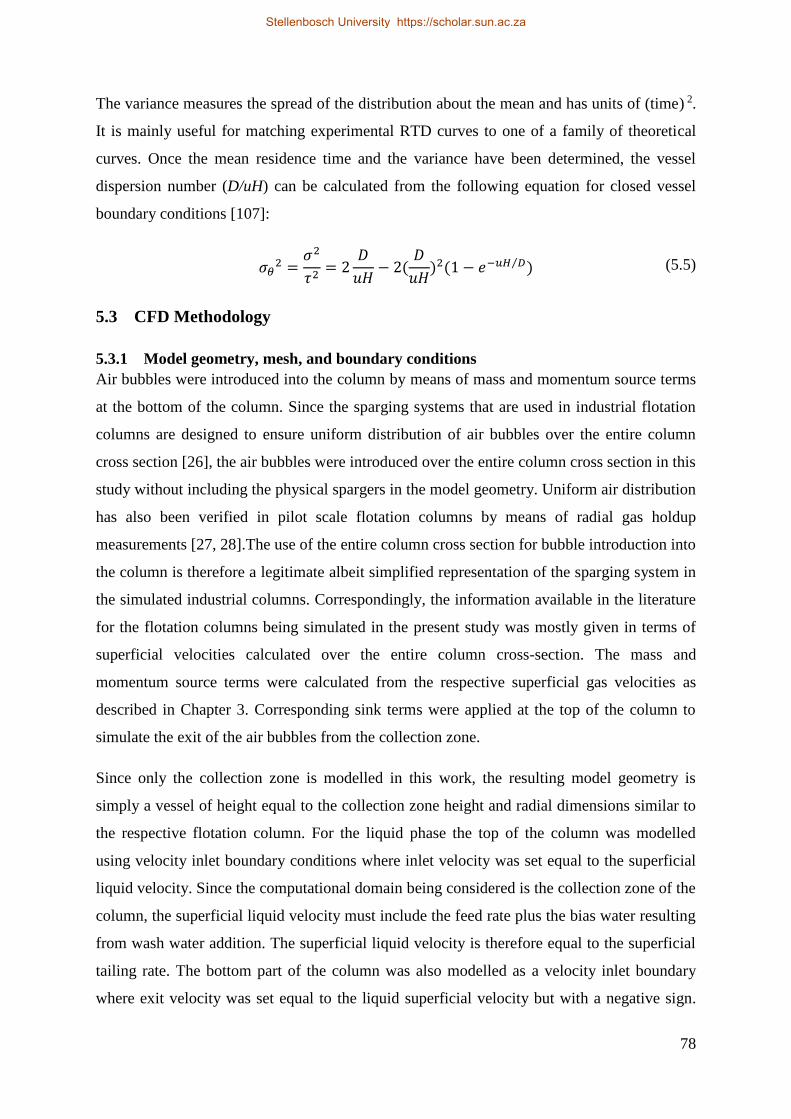
78
The variance measures the spread of the distribution about the mean and has units of (time) 2.
It is mainly useful for matching experimental RTD curves to one of a family of theoretical
curves. Once the mean residence time and the variance have been determined, the vessel
dispersion number (D/uH) can be calculated from the following equation for closed vessel
boundary conditions [107]:
𝜎𝜃
2 =𝜎2
𝜏2= 2
𝐷
𝑢𝐻− 2(
𝐷
𝑢𝐻)2(1 − 𝑒−𝑢𝐻 𝐷⁄ ) (5.5)
5.3 CFD Methodology
5.3.1 Model geometry, mesh, and boundary conditions
Air bubbles were introduced into the column by means of mass and momentum source terms
at the bottom of the column. Since the sparging systems that are used in industrial flotation
columns are designed to ensure uniform distribution of air bubbles over the entire column
cross section [26], the air bubbles were introduced over the entire column cross section in this
study without including the physical spargers in the model geometry. Uniform air distribution
has also been verified in pilot scale flotation columns by means of radial gas holdup
measurements [27, 28].The use of the entire column cross section for bubble introduction into
the column is therefore a legitimate albeit simplified representation of the sparging system in
the simulated industrial columns. Correspondingly, the information available in the literature
for the flotation columns being simulated in the present study was mostly given in terms of
superficial velocities calculated over the entire column cross-section. The mass and
momentum source terms were calculated from the respective superficial gas velocities as
described in Chapter 3. Corresponding sink terms were applied at the top of the column to
simulate the exit of the air bubbles from the collection zone.
Since only the collection zone is modelled in this work, the resulting model geometry is
simply a vessel of height equal to the collection zone height and radial dimensions similar to
the respective flotation column. For the liquid phase the top of the column was modelled
using velocity inlet boundary conditions where inlet velocity was set equal to the superficial
liquid velocity. Since the computational domain being considered is the collection zone of the
column, the superficial liquid velocity must include the feed rate plus the bias water resulting
from wash water addition. The superficial liquid velocity is therefore equal to the superficial
tailing rate. The bottom part of the column was also modelled as a velocity inlet boundary
where exit velocity was set equal to the liquid superficial velocity but with a negative sign.
Stellenbosch University https://scholar.sun.ac.za

79
For the column wall, no slip boundary conditions were applied for both the liquid (primary
phase) and the air bubbles as well as solids (secondary phases).
The mesh used in the present study was generated over the model geometry using the
meshing application of ANSYS Workbench. The mesh was in each case generated using the
Sweep method which creates a mesh comprising mainly hexahedral elements. The
computational mesh for the square and the cylindrical columns are shown in Figure 5.1 and
Figure 5.2, respectively. Grid independency studies were conducted in which the numerical
solution was tested at several different mesh sizes until changes in applicable flow regimes
became insignificant.
Figure 5.1: Computational mesh for the 0.45 m square column (side view).
Stellenbosch University https://scholar.sun.ac.za
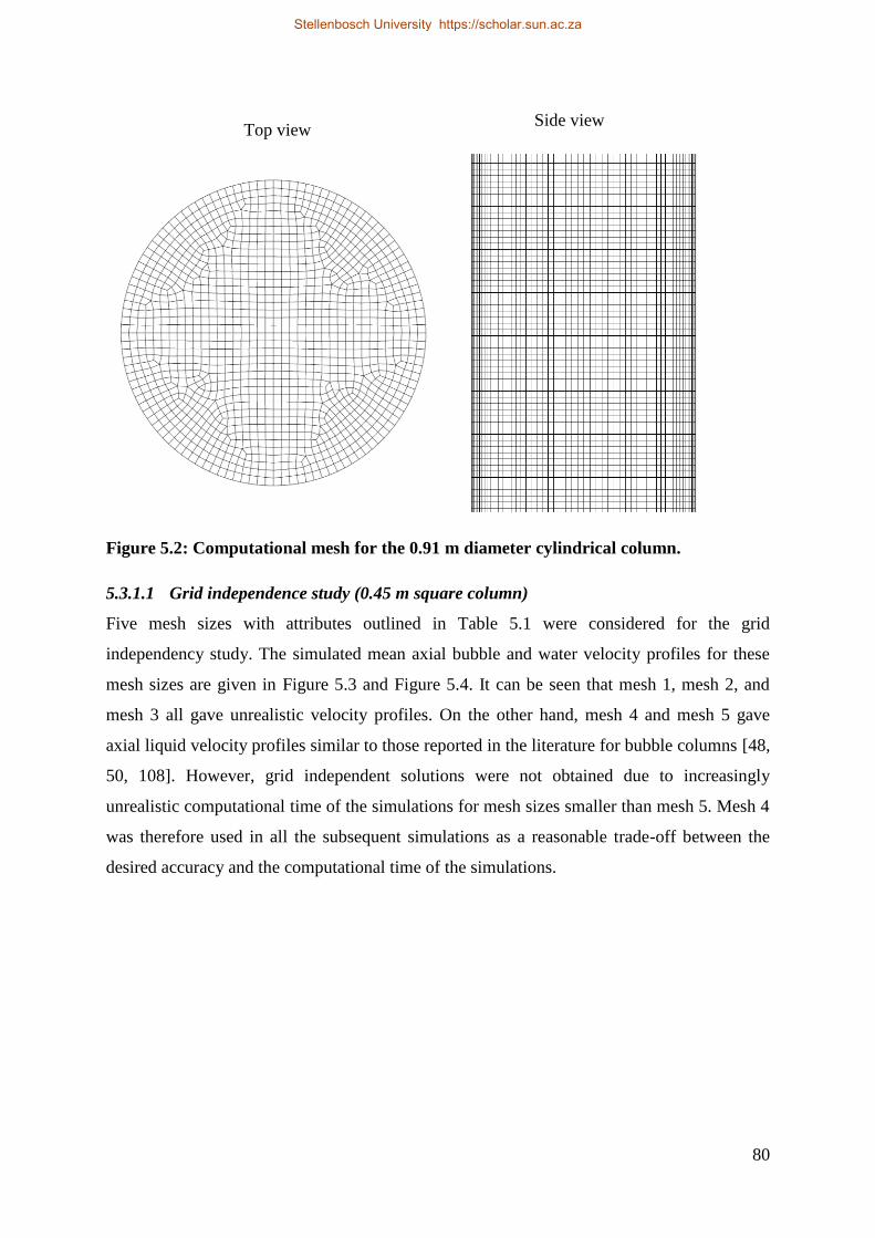
80
Figure 5.2: Computational mesh for the 0.91 m diameter cylindrical column.
5.3.1.1 Grid independence study (0.45 m square column)
Five mesh sizes with attributes outlined in Table 5.1 were considered for the grid
independency study. The simulated mean axial bubble and water velocity profiles for these
mesh sizes are given in Figure 5.3 and Figure 5.4. It can be seen that mesh 1, mesh 2, and
mesh 3 all gave unrealistic velocity profiles. On the other hand, mesh 4 and mesh 5 gave
axial liquid velocity profiles similar to those reported in the literature for bubble columns [48,
50, 108]. However, grid independent solutions were not obtained due to increasingly
unrealistic computational time of the simulations for mesh sizes smaller than mesh 5. Mesh 4
was therefore used in all the subsequent simulations as a reasonable trade-off between the
desired accuracy and the computational time of the simulations.
Top view Side view
Stellenbosch University https://scholar.sun.ac.za

81
Table 5.1: Mesh sizes considered for the grid independency study (0.45 m square
column).
Identification Element size
(cm)
Number of
cells
Number of
nodes
Minimum
orthogonal
quality
Gas
holdup
(%)
Mesh 1 5 19, 200 23, 353 1 13.07
Mesh 2 3.5 53, 508 61, 650 1 13.01
Mesh 3 2.5 123, 768 138, 263 1 12.56
Mesh 4 1.75 367, 744 397, 305 1 13.43
Mesh 5 1.25 986, 256 1, 043, 178 1 13.24
Figure 5.3: Simulated mean axial bubble velocities for different mesh sizes (0.45 m
square column).
-0,1
-0,05
0
0,05
0,1
0,15
0,2
0,25
0,3
-0,25 -0,2 -0,15 -0,1 -0,05 0 0,05 0,1 0,15 0,2 0,25
Me
an a
xial
bu
bb
le v
elo
city
(m
/s)
Radial position (m)
Mesh 1 Mesh 2 Mesh 3 Mesh 4 Mesh 5
Stellenbosch University https://scholar.sun.ac.za
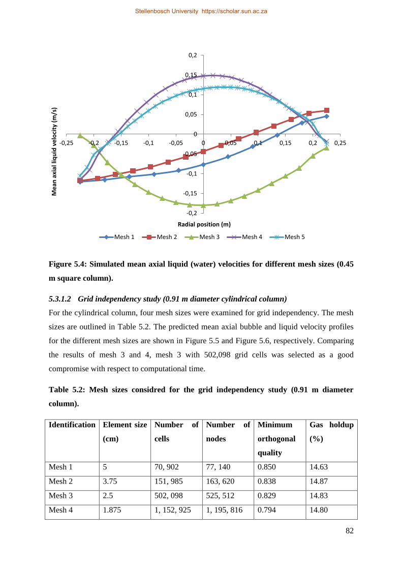
82
Figure 5.4: Simulated mean axial liquid (water) velocities for different mesh sizes (0.45
m square column).
5.3.1.2 Grid independency study (0.91 m diameter cylindrical column)
For the cylindrical column, four mesh sizes were examined for grid independency. The mesh
sizes are outlined in Table 5.2. The predicted mean axial bubble and liquid velocity profiles
for the different mesh sizes are shown in Figure 5.5 and Figure 5.6, respectively. Comparing
the results of mesh 3 and 4, mesh 3 with 502,098 grid cells was selected as a good
compromise with respect to computational time.
Table 5.2: Mesh sizes considred for the grid independency study (0.91 m diameter
column).
Identification Element size
(cm)
Number of
cells
Number of
nodes
Minimum
orthogonal
quality
Gas holdup
(%)
Mesh 1 5 70, 902 77, 140 0.850 14.63
Mesh 2 3.75 151, 985 163, 620 0.838 14.87
Mesh 3 2.5 502, 098 525, 512 0.829 14.83
Mesh 4 1.875 1, 152, 925 1, 195, 816 0.794 14.80
-0,2
-0,15
-0,1
-0,05
0
0,05
0,1
0,15
0,2
-0,25 -0,2 -0,15 -0,1 -0,05 0 0,05 0,1 0,15 0,2 0,25
Me
an a
xial
liq
uid
ve
loci
ty (
m/s
)
Radial position (m)
Mesh 1 Mesh 2 Mesh 3 Mesh 4 Mesh 5
Stellenbosch University https://scholar.sun.ac.za
83
Figure 5.5: Simulated mean axial bubble velocity profiles for the different mesh sizes
(0.91 m diameter column).
-0,15
-0,1
-0,05
0
0,05
0,1
0,15
0,2
0,25
0,3
0,35
-0,6 -0,4 -0,2 0 0,2 0,4 0,6
Me
an a
xial
bu
bb
le v
elo
city
(m
/s)
Radial position (m)
Mesh 1 Mesh 2 Mesh 3 Mesh 4
Stellenbosch University https://scholar.sun.ac.za

84
Figure 5.6: Simulated mean axial liquid velocity profiles for the different mesh sizes
(0.91 m diameter column).
5.3.2 Multiphase model
In this research, the multiphase flow in the flotation columns was modeled using the
Eulerian-Eulerian (E-E) approach which has been recommended for industrial scale bubble
columns due to its computational efficiency [80, 109]. In the Eulerian-Eulerian approach,
both the continuous (primary) phase and the dispersed (secondary) phase are modelled in an
Eulerian frame of reference as interpenetrating continua. Conservation equations for mass
and momentum are therefore solved for each phase separately. Interaction between the phases
is then accounted for by means of momentum exchange terms incorporated in their respective
momentum equations.
In the present study, the three-phase flow in the industrial flotation columns was modelled
considering water as the continuous phase (or primary phase) while air bubbles and solid
particles were treated as dispersed phases (or secondary phases). The volume averaged mass
and momentum conservation equations for the gas and liquid phase have been given in
Chapter 3, equations (3.3) and (3.4). The continuity and momentum equations for the solids
(particles) are presented respectively as follows:
-0,25
-0,2
-0,15
-0,1
-0,05
0
0,05
0,1
0,15
0,2
-0,6 -0,4 -0,2 0 0,2 0,4 0,6
Me
an a
xial
liq
uid
(w
ate
r) v
elo
city
(m
/s)
Radial position (m)
Mesh 1 Mesh 2 Mesh 3 Mesh 4
Stellenbosch University https://scholar.sun.ac.za

85
𝜕
𝜕𝑡(휀𝑠𝜌𝑠) + 𝛻. (휀𝑠𝜌𝑠𝒖𝑠⃗⃗⃗⃗ ) = 0 (5.6)
𝜕
𝜕𝑡(휀𝑠𝜌𝑠𝒖𝑠⃗⃗⃗⃗ ) + 𝛻. (휀𝑠𝜌𝑠𝒖𝑠⃗⃗⃗⃗ ⊗ 𝒖𝑠⃗⃗⃗⃗ ) = −휀𝑠𝛻𝑝 − ∇𝑃𝑠 + 𝛻. 휀𝑠𝜏�̿� + 휀𝑠𝜌𝑠�⃗⃗� + 𝑀𝑠,𝑙 (5.7)
where s is the index for solid phase and Ps is the solids pressure, εs is the volume fraction, ρs
is the phase density, and 𝒖𝑠⃗⃗⃗⃗ is the velocity of the solid phase. 𝑀𝑠,𝑙 is the momentum exchange
between the solids and liquid phases and ερg is the gravity force, while τ�̿� is the solids phase
stress tensor given by:
𝜏�̿� = 휀𝑠𝜇𝑠(𝛻𝒖𝑠⃗⃗⃗⃗ + 𝛻𝒖𝑠⃗⃗⃗⃗
𝑇) + 휀𝑠 (𝜆𝑠 −
2
3𝜇𝑠) 𝛻. 𝒖𝑠⃗⃗⃗⃗ 𝐼 ̿ (5.8)
In terms of the momentum exchange forces between the phases, only the drag force between
the continuous phase and the dispersed phases was considered in this study. The momentum
exchange between the two dispersed phases was not included in the model.
5.3.2.1 Gas-liquid drag force
The drag force per unit volume for bubbles in a swarm is generally obtained from the
following equation:
𝐹𝐷⃗⃗ ⃗⃗ (𝑔, 𝑙) =
3휀𝑔휀𝑙
4(𝜌𝑙
𝑑𝐵) 𝐶𝐷(𝑔, 𝑙)|𝒖𝑔⃗⃗ ⃗⃗ − 𝒖𝑙⃗⃗⃗⃗ |(𝒖𝑔⃗⃗ ⃗⃗ − 𝒖𝑙⃗⃗⃗⃗ ) (5.9)
where CD (g, l) is the drag coefficient between the liquid phase and the air bubbles, dB is the
bubble diameter, and 𝒖𝑔⃗⃗ ⃗⃗ − 𝒖𝑙⃗⃗⃗⃗ is the slip velocity. There are a number of empirical
correlations that can be used to calculate the drag coefficient, CD (g, l). The drag coefficient is
normally presented in these correlations as a function of the bubble Reynolds number (Re)
defined as:
𝑅𝑒 =
𝜌𝑙|𝒖𝑔⃗⃗ ⃗⃗ − 𝒖𝑙⃗⃗⃗⃗ |𝑑𝐵
𝜇𝑙 (5.10)
In this study, the drag coefficient was calculated using the Universal Drag Laws [94]. In this
case, the universal drag coefficient is defined in different ways depending on whether the
prevailing regime is in the viscous regime category, the distorted bubble regime, or the
strongly deformed caped bubbles regime. At the moderate superficial gas velocities simulated
Stellenbosch University https://scholar.sun.ac.za

86
in the present study, the viscous regime conditions apply and the drag coefficient is
calculated from the following equation:
𝐶𝐷(𝑔, 𝑙)𝑣𝑖𝑠 =
24
𝑅𝑒(1 + 0.1𝑅𝑒0.75) (5.11)
5.3.2.2 Liquid-solid drag force
The drag force between the liquid and the solid particles was calculated using the Wen and
Yu model [110]. The drag force per unit volume is given by:
𝐹𝐷⃗⃗ ⃗⃗ (𝑠, 𝑙) =
3
4𝐶𝐷(𝑠, 𝑙)
휀𝑠휀𝑙𝜌𝑙|𝒖𝑠⃗⃗⃗⃗ − 𝒖𝑙⃗⃗⃗⃗ |
𝑑𝑠휀𝑙
−2.65(𝒖𝑙⃗⃗⃗⃗ − 𝒖𝑠⃗⃗⃗⃗ ) (5.12)
The drag coefficient is calculated as:
𝐶𝐷(𝑠, 𝑙) =
24
휀𝑙𝑅𝑒𝑠
[1 + 0.15(휀𝑙𝑅𝑒𝑠)0.687] (5.13)
The Wen and Yu model is suitable for dilute systems similar to the conditions simulated in
the present study.
5.3.3 Turbulence model
Turbulence in the continuous phase (water) was modelled using the realizable k-ϵ turbulence
model which is a RANS (Reynolds-Averaged Navier-Stokes) based model. In the RANS
turbulence modelling, the instantaneous Navier-Stokes equations are time averaged to
produce the Reynolds-Averaged Navier-Stokes (RANS) equations which are solved to obtain
a time averaged flow field. The averaging procedure introduces additional unknowns; the
Reynolds stresses which represent the effects of turbulent fluctuations on the mean flow.
RANS models therefore calculate the mean flow while modelling the effect of turbulent
fluctuations on the mean flow.
The k-ϵ model is an Eddy Viscosity turbulence model. The Reynolds stresses are therefore
related to the velocity gradients through the turbulent viscosity as presented in the following
equation:
−𝜌𝑢𝑖
′𝑢𝑗′ = 𝜇𝑡 (
𝜕𝒖𝑖
𝜕𝑥𝑗+
𝜕𝒖𝑗
𝜕𝑥𝑖) −
2
3(𝜌𝑘 + 𝜇𝑡
𝜕𝒖𝑘
𝜕𝑥𝑖) 𝛿𝑖𝑗 (5.14)
where μt is the turbulent or eddy viscosity, k is the turbulent kinetic energy and δij is the
Kronecker delta. The Kronecker delta is important in order to make the eddy viscosity
Stellenbosch University https://scholar.sun.ac.za
87
concept applicable to normal stresses where i = j. On the other hand, the turbulent viscosity is
calculated from the turbulent kinetic energy (k) and the turbulent dissipation rate according to
the following equation:
𝜇𝑡 = 𝜌𝐶𝜇
𝑘2
𝜖 (5.15)
The k-ϵ model is therefore a two equation turbulence model since two additional transport
equations must be solved for the turbulent kinetic energy (k) and dissipation rates (ϵ).
5.3.4 Residence Time Distribution (RTD) Simulation
There are several methods for predicting residence time distribution using CFD. One way is
to represent the tracer fluid by a large number of discrete particles and then applying
Lagrangian particle tracking analysis with the Discrete Phase Model (DPM) available in
ANYSIS FLUENT [111, 112]. The particle residence time is monitored at the outlet and
plotted in a histogram which represents the residence time distribution. This method was not
used in the present study because it requires a larger number of particles with subsequent
increase in the computational cost of the simulations.
In the second method, the tracer fluid is considered as a continuum by solving an additional
transport equation for the tracer species. The concentration of the tracer is then monitored at
the outlet to give the RTD. The method applied to simulate the liquid RTD in the present
study is similar to this one.
5.3.4.1 Liquid RTD
Liquid RTD was modelled by solving conservation equations for chemical tracer species
using the Species Model in ANSYS FLUENT. In multiphase flows, the species conservation
equation is solved for each phase q to predict the local mass fraction of each species 𝑌𝑖𝑞 by
means of a convection-diffusion equation for the ith species. For an inert tracer species, the
species conservation equation for a multiphase mixture can be represented as follows:
𝜕
𝜕𝑡(𝜌𝑞휀𝑞𝑌𝑖
𝑞) + ∇. (𝜌𝑞휀𝑞 �⃗⃗� 𝑞𝑌𝑖𝑞) = −∇. 휀𝑞𝐽𝑖⃗⃗
𝑞 (5.16)
where 𝐽𝑖⃗⃗ is the diffusion flux of species i which is obtained from the following equation:
𝐽𝑖⃗⃗ = −(𝜌𝐷𝑖,𝑚 +
𝜇𝑡
𝑆𝑐𝑡) ∇𝑌𝑖 (5.17)
Stellenbosch University https://scholar.sun.ac.za

88
where Di,m is the mass diffusion coefficient for species i, Sct is the turbulent Schmidt number
(𝜇𝑡
𝜌𝐷𝑡 where μt is the turbulent viscosity) and Dt is the turbulent diffusivity. The flux 𝐽𝑖⃗⃗
therefore consists of two parts, the molecular diffusion and the turbulent diffusion.
In the present study, the simulations were conducted in two stages. First, the velocity flow
field was calculated using the First Order Upwind scheme for momentum, volume fraction,
and turbulence kinetic energy and dissipation rate discretization. The First Order Upwind
scheme was preferred in order to avoid divergence during the computations.
In the second stage, tracer simulations were performed on the ‘frozen’ velocity field obtained
in the first step. In other words, once the converged solution of the flow equations was
obtained, the flow field was ‘frozen’ by disabling the flow equations and the turbulence and
volume fraction equations in the solver. A tracer species was then defined with properties
similar to those of the carrier fluid, in this case water. Next, unsteady tracer simulations were
carried out solving only the species conservation equation using the Second Order Implicit
formulation for time discretization.
5.3.4.1.1 Tracer injection and monitoring
The tracer mass fraction at the column inlet was set to 1 for time durations similar to the
tracer injection time in the respective experimental columns. In this case, the total injection
time was about 30 seconds for the square column [58] and 1 second for the cylindrical
column [65]. After that, the mass fraction of the tracer was again set to 0 and the simulation
continued. The mass fraction of the tracer was subsequently recorded at the outlet every 10s
and used to obtain the Residence Time Distribution (RTD) curves from which the mean
residence time (τ) and the vessel dispersion number (Nd) were calculated.
The method used for liquid RTD simulation is summarized as follows:
Calculate velocity field – Calculated using the First Order Upwind momentum
discretization scheme
Introduce Tracer Species – A tracer species is introduced having properties of water,
the carrier fluid
Perform unsteady tracer simulation – Species conservation equation is solved on
frozen flow field while monitoring exit mass fraction
Stellenbosch University https://scholar.sun.ac.za
89
5.3.4.2 Particle (Solids) RTD
Particle RTD was modelled using a transport equation that computes the age of particles in
the column. This method is based on the transport equation for the local residence time of a
fluid as derived by Ghirelli and Leckner [35]. The equation was introduced into the CFD
model of the flotation column as a User Defined Scalar (UDS) equation. In this case, particle
age (or residence time) is considered as a scalar property that is being transported by the
particles. The resulting spatial distribution of particle age in the column can be used to
describe the mixing characteristics of the solid phase. The transport equation for the age of
particles is presented as follows:
𝜕
𝜕𝑡(𝜌𝑠휀𝑠𝑎𝑠) +
𝜕
𝜕𝑥𝑖
(𝜌𝑠𝒖𝑖휀𝑠𝑎𝑠) = 𝜌𝑠휀𝑠 (5.18)
The product on the right hand side of equation (5.18) was included as a source term
introduced by means of a User Defined Function (UDF). The UDF is outlined in Appendix 2.
The boundary conditions for the particle age were set up as follows:
At the inlet the particle age (or residence time) is set to zero
At the walls, a zero flux condition was specified for the particle age
At the outlet, the particle age was extrapolated from the last domain cell
The mean residence time of the particles was obtained as the mass weighted or area weighted
average age of the particles at the outlet. An overview of the method is presented in the
following outline:
Calculate velocity field – First Order Upwind scheme is used for momentum
discretization
Introduce UDS for particle age – Particle age is considered as a scalar property
transported by the particles
Solve UDS equation – Scalar conservation equation for spatial age distribution is
solved on ‘frozen’ flow field
Determine Residence time – Mass Weighted Average age at outlet is the mean
residence time
Stellenbosch University https://scholar.sun.ac.za
90
5.4 Results and discussion
Three phase CFD simulations were conducted to model the 0.45 m square column and the
0.91 m diameter cylindrical column that were used in the work of Dobby and Finch [58] and
Yianatos and Bergh [65], respectively. The operating conditions of the two columns are
presented in theTable 5.3.
A bubble size of 1 mm was used in the simulations for the 0.45 m column since this is the
typical bubble size reported for this column in literature [1]. On the other hand, the 0.91 m
diameter column was simulated with different average bubble sizes including 0.8, 1, 1.5 and
2 mm in order to determine the bubble size that would give the correct gas holdup (18%) for
the column (refer to Table 5.3). The correct gas holdup was subsequently obtained with a
bubble size of 0.8 mm. The simulated RTDs obtained using the different bubble sizes were
also compared in order to investigate the effect of bubble size on axial mixing in the column.
The CFD simulations in this study were conducted using average particle sizes comparable
with the range of particle sizes studied in the corresponding experimental work. Separate
simulations were performed for each particle size in order to minimize the computational cost
of the simulations. The results obtained from the CFD simulations are presented separately
for the two columns.
Table 5.3: Operating conditions of the industrial columns being simulated in the present
study [58, 65].
Square column (Dobby and
Finch)
Cylindrical column
(Yianatos and Bergh)
Superficial gas velocity
(cm/s) 1.4 1.8
Superficial liquid velocity
(cm/s) 1.2 0.92
Gas holdup (%) 5.5 18
Feed wt% solids 3 16.2
Solids volume fraction 0.006 0.0604
Solids density (g/cm3) 5.19 3
Collection zone height (m) 9.5 10
Stellenbosch University https://scholar.sun.ac.za
91
5.4.1 Square column
In their experimental work, Dobby and Finch [58] measured the liquid (water) RTD together
with the solids RTD for a range of solid particle sizes averaging 44, 63, 88, and 125 µm. In
the present research, CFD modelling was applied to simulate the operating conditions
prevailing in the experimental column. Separate simulations were carried out for each of the
particle sizes, i.e., using one size of particles at a time.
5.4.1.1 Liquid residence time distribution (RTD)
The Residence Time Distribution (RTD) obtained from CFD simulation is compared with the
experimental RTD in Figure 5.7. Since the dominant particle size (d80) for the modelled
column was mostly particles of about 45 µm size [2], the CFD results that were compared
with the experimental liquid RTD are those that were run with the 44 µm average particle
size. The CFD results compare favourably with the experimental data as shown in Figure 5.7.
The mixing parameters calculated from the CFD simulated liquid RTD, together with the
predicted air holdup are compared with the literature experimental data inTable 5.4. Both the
liquid mean residence time and the vessel dispersion number are reasonably well predicted by
the CFD simulations. However, the predicted air holdup is larger than the measured one.
Dobby and Finch [58] also noted that the measured air holdup was smaller than would be
expected for bubbles of approximately 1 mm size. However, the reason for the small air
holdup value is not clear from their experimental data. One of the possible reasons could be
that the experimental air holdup was probably measured near the bottom of the column in
which case the air holdup would be smaller than the average holdup in the entire column
considering the axial gas holdup variation.
Stellenbosch University https://scholar.sun.ac.za

92
Figure 5.7: Simulated liquid (water) RTD for the square column compared with the
experimental data of Dobby and Finch [58].
Table 5.4: Comparison of CFD predicted mixing parameters with experimental data.
Parameter CFD Prediction Experimental data[58]
Liquid mean residence time
(𝜏𝑙) in minutes 11.4 12.6
Vessel dispersion number
(Nd) 0.209 0.278
Estimated air holdup, εg 0.130 0.055
5.4.1.2 Particle (solids) RTD
Solving the transport equation of the particle age in the column gives the spatial distribution
of the age of the particles in the collection zone of the column. The spatial age distribution of
44 µm solids is presented in Figure 5.8 for illustration. The simulated particle age seems to
increase from the walls towards the centre of the column. This is as a result of the liquid
circulation pattern in which the liquid (water) rises in the centre of the column and descends
near the walls. The axial velocity profile of water at the mid-height position in the column is
presented in Figure 5.9. It can be seen that the velocity is positive in the centre and negative
0
0,1
0,2
0,3
0,4
0,5
0,6
0,7
0,8
0,9
1
0 0,5 1 1,5 2 2,5 3 3,5
Dim
en
sio
nle
ss R
TD E
(ϴ)
Dimensionless Time (ϴ)
Experimental (Dobby and Finch 1985)
CFD Simulation
Stellenbosch University https://scholar.sun.ac.za

93
near the walls of the column. The water is therefore rising in the centre and descending at the
walls. The rising water carries with it ‘older’ particles that had reached the bottom part of the
column while the descending water carries with it the ‘younger’ particles entering the column
at the top. The particle age distribution in the column is therefore governed by the established
liquid circulation prevailing in the column. The implication of these observations is that the
back-mixing effect resulting from liquid circulation in flotation columns might cause short-
circuiting of feed to gangue flow as earlier suggested by Xia et al. [15]. Gangue might also
flow back to feed or concentrate flow and thus make separation less selective.
Figure 5.8: Contours of simulated particle age distribution in the square column;
particle size = 44 µm.
Stellenbosch University https://scholar.sun.ac.za

94
Figure 5.9: Axial velocity profile of water showing the circulation pattern with upward
flow at the centre and downward flow near the column walls (square column).
The area weighted average or mass weighted average age of the particles at the outlet of the
column gives the particle mean residence time. In Figure 5.10, the particle mean residence
times obtained from the CFD simulations using the particle age scalar equation are compared
with the experimental values reported by Dobby and Finch [58]. The Mean Absolute Relative
Error (MARE) between the CFD predictions and the experimental data was calculated from
the following equation:
𝑀𝐴𝑅𝐸(%) = 100
1
𝑁𝛴 |1 −
𝜏𝐶𝐹𝐷
𝜏𝐸𝑥𝑝.| (5.19)
With Mean Absolute Relative Error (MARE) equal to 7.8% the CFD results compared well
with the experimental data. The simulation results in Figure 5.10 also show that the solids
(particle) mean residence time decreases with increasing particle size. This is also evident in
the corresponding experimental data. In comparison with the simulated liquid mean residence
time of 11.4 minutes (refer to Table 5.4), the predicted mean residence time of 5 minutes for
the largest particle size (125 µm) was about 50% of the liquid residence time. On the other
-0,3
-0,25
-0,2
-0,15
-0,1
-0,05
0
0,05
0,1
0,15
-0,25 -0,2 -0,15 -0,1 -0,05 0 0,05 0,1 0,15 0,2 0,25
Axi
al W
ate
r V
elo
city
(m
/s)
Radial Position (m)
Stellenbosch University https://scholar.sun.ac.za

95
hand, the smallest particle size (44 µm) had mean residence time (10.3 minutes) similar to the
liquid one.
Figure 5.10: Comparison of CFD predicted (simulation) and experimental
measurements [58] of particle mean residence time vs particle size.
5.4.1.3 Comparison of liquid (water) and solids flow patterns
A comparison of the liquid and solids axial velocity profiles was undertaken as illustrated in
Figure 5.11 and Figure 5.12 in order to determine whether the solids dispersion number and
the liquid one were equivalent as suggested by previous researchers [58, 65, 104]. The axial
velocity profiles were taken at the mid-height position in the column. In Figure 5.11, the axial
velocity profile of 88 µm solids is compared with the liquid one. It can be observed that the
negative part (downward part) of the solids axial velocity is slightly larger than the liquid one
while the positive solids velocity (upward part) is less than the liquid one. This is due to the
gravitational settling imposed on the solid particles. However, the differences in the velocities
of the phases are not large enough to suggest significant differences in their axial mixing. It is
therefore reasonable for column flotation design and scale up purposes to assume the equality
of the liquid and solids vessel dispersion numbers for this particular particle size.
0
2
4
6
8
10
12
14
20 40 60 80 100 120 140
Par
ticl
e m
ean
re
sid
en
ce t
ime
(M
inu
tes)
Particle size (µm)
Experimental
CFD Simulation
Stellenbosch University https://scholar.sun.ac.za
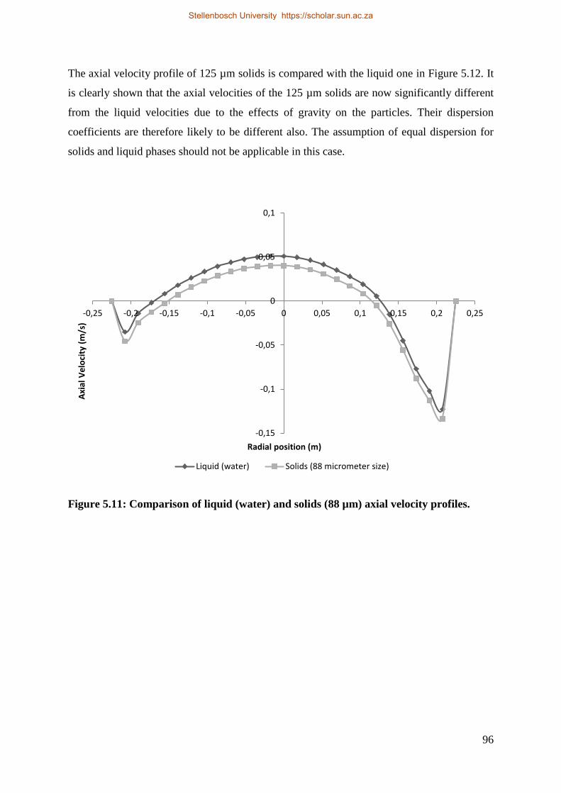
96
The axial velocity profile of 125 µm solids is compared with the liquid one in Figure 5.12. It
is clearly shown that the axial velocities of the 125 µm solids are now significantly different
from the liquid velocities due to the effects of gravity on the particles. Their dispersion
coefficients are therefore likely to be different also. The assumption of equal dispersion for
solids and liquid phases should not be applicable in this case.
Figure 5.11: Comparison of liquid (water) and solids (88 µm) axial velocity profiles.
-0,15
-0,1
-0,05
0
0,05
0,1
-0,25 -0,2 -0,15 -0,1 -0,05 0 0,05 0,1 0,15 0,2 0,25
Axi
al V
elo
city
(m
/s)
Radial position (m)
Liquid (water) Solids (88 micrometer size)
Stellenbosch University https://scholar.sun.ac.za
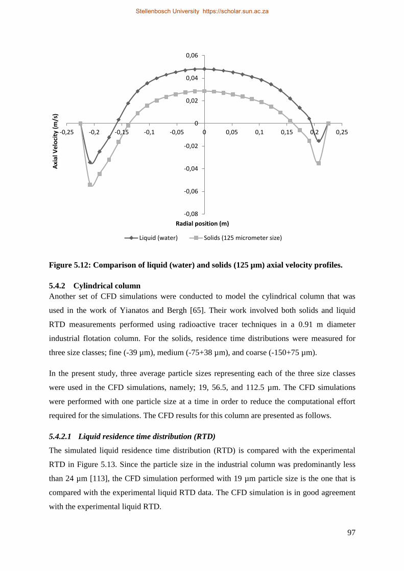
97
Figure 5.12: Comparison of liquid (water) and solids (125 µm) axial velocity profiles.
5.4.2 Cylindrical column
Another set of CFD simulations were conducted to model the cylindrical column that was
used in the work of Yianatos and Bergh [65]. Their work involved both solids and liquid
RTD measurements performed using radioactive tracer techniques in a 0.91 m diameter
industrial flotation column. For the solids, residence time distributions were measured for
three size classes; fine (-39 µm), medium (-75+38 µm), and coarse (-150+75 µm).
In the present study, three average particle sizes representing each of the three size classes
were used in the CFD simulations, namely; 19, 56.5, and 112.5 µm. The CFD simulations
were performed with one particle size at a time in order to reduce the computational effort
required for the simulations. The CFD results for this column are presented as follows.
5.4.2.1 Liquid residence time distribution (RTD)
The simulated liquid residence time distribution (RTD) is compared with the experimental
RTD in Figure 5.13. Since the particle size in the industrial column was predominantly less
than 24 µm [113], the CFD simulation performed with 19 µm particle size is the one that is
compared with the experimental liquid RTD data. The CFD simulation is in good agreement
with the experimental liquid RTD.
-0,08
-0,06
-0,04
-0,02
0
0,02
0,04
0,06
-0,25 -0,2 -0,15 -0,1 -0,05 0 0,05 0,1 0,15 0,2 0,25
Axi
al V
elo
city
(m
/s)
Radial position (m)
Liquid (water) Solids (125 micrometer size)
Stellenbosch University https://scholar.sun.ac.za

98
The mixing parameters (liquid mean residence time and vessel dispersion number) calculated
from the CFD simulated liquid RTD, together with the predicted air holdup are compared
with the experimental data of Yianatos and Bergh [65] in Table 5.5. It can be seen that the
simulated mixing parameters are in reasonable agreement with the experimental data.
Figure 5.13: Simulated liquid (water) RTD for the cylindrical column compared with
the experimental data of Yianatos and Bergh [65].
Table 5.5: Comparison of CFD predicted (simulated) mixing parameters with
experimental data.
Parameter CFD prediction Experimental data [65]
Liquid mean residence time
in minutes (𝜏𝑙)
15.5 14.3
Relative variance (𝜎𝜃2) 0.561 0.515
Vessel dispersion number
(Nd)
0.488 0.41
Gas holdup, εg (%) 17.6 18
0
0,1
0,2
0,3
0,4
0,5
0,6
0,7
0,8
0,9
1
0 0,5 1 1,5 2 2,5 3 3,5 4
Dim
en
sio
nle
ss R
TD E
(ϴ)
Dimensionless time (ϴ)
Experimental (Yianatos and Bergh 1992)
CFD Simulation
Stellenbosch University https://scholar.sun.ac.za

99
5.4.2.1.1 Effect of particle size and bubble size on liquid axial mixing
The effect of particle size on the liquid vessel dispersion number was investigated using
liquid RTDs obtained from CFD simulations performed with different particle sizes. The
results are shown in Figure 5.14 for simulations conducted with two different bubble sizes;
0.8 and 1 mm. It can be seen that increasing the particle size results in a decrease in the liquid
vessel dispersion number. On the other hand, previous studies had found that increasing the
percentage of solids (wt %) in the feed caused a slight decrease in the liquid mixing intensity
inside the column [59, 114, 115]. In other words the liquid vessel dispersion number
decreased with increasing solids percentage in the feed (or increasing pulp density).
Subsequently, the feed solids percentage has been included in the empirical correlations that
are used for estimating the vessel dispersion number for predicting the recovery in column
scale up procedures. However, the decrease in liquid dispersion number observed in the
present research as particle size increases suggests that particle size should also be considered
in the correlations for estimating the vessel dispersion number. This way the effect of particle
size on mineral recovery will also be accounted for in the scale up procedure.
Figure 5.14 also shows that increasing bubble size caused reduction in the liquid dispersion.
A similar observation was reported by Xia et al. [15] who observed that a reduction in bubble
size resulted in a rise in the axial liquid velocity. The increase in liquid back-mixing can be
attributed to the increase in gas holdup resulting from the reduction in bubble size. As the
bubble size is reduced, the number of bubbles increases while the bubble rise velocity
reduces causing an increase in bubble residence time. The subsequent increase in gas holdup
results in higher axial liquid velocity which will cause a stronger back-mixing effect [15, 59].
The effect of bubble size on liquid dispersion is further illustrated in Figure 5.15. The liquid
vessel dispersion number decreased from 0.488 to 0.281 when the bubble size was increased
from 0.8 mm to 1mm, which is almost a 50% decrease. This is an important finding
especially with regard to fine particles flotation where micro bubbles have been suggested to
improve the collection efficiency of the fine particles. Using micro bubbles may therefore not
necessarily result in improved fine particles recovery because of the increase in liquid back-
mixing.
Stellenbosch University https://scholar.sun.ac.za

100
Figure 5.14: Effect of particle size on the liquid vessel dispersion number. The results
are from CFD simulations performed with two different bubble sizes, namely 0.8 and 1
mm (cylindrical column).
Figure 5.15: Effect of bubble size on the liquid vessel dispersion number (cylindrical
column).
0
0,1
0,2
0,3
0,4
0,5
0,6
0 20 40 60 80 100 120
Liq
uid
ves
sel d
isp
ersi
on
nu
mb
er
Particle size (µm)
0.8 mm bubble size 1 mm bubble size
0,488
0,281
0
0,1
0,2
0,3
0,4
0,5
0,6
0,8 1
Ve
sse
l dis
pe
rsio
n n
um
be
r
Bubble size (mm)
Stellenbosch University https://scholar.sun.ac.za
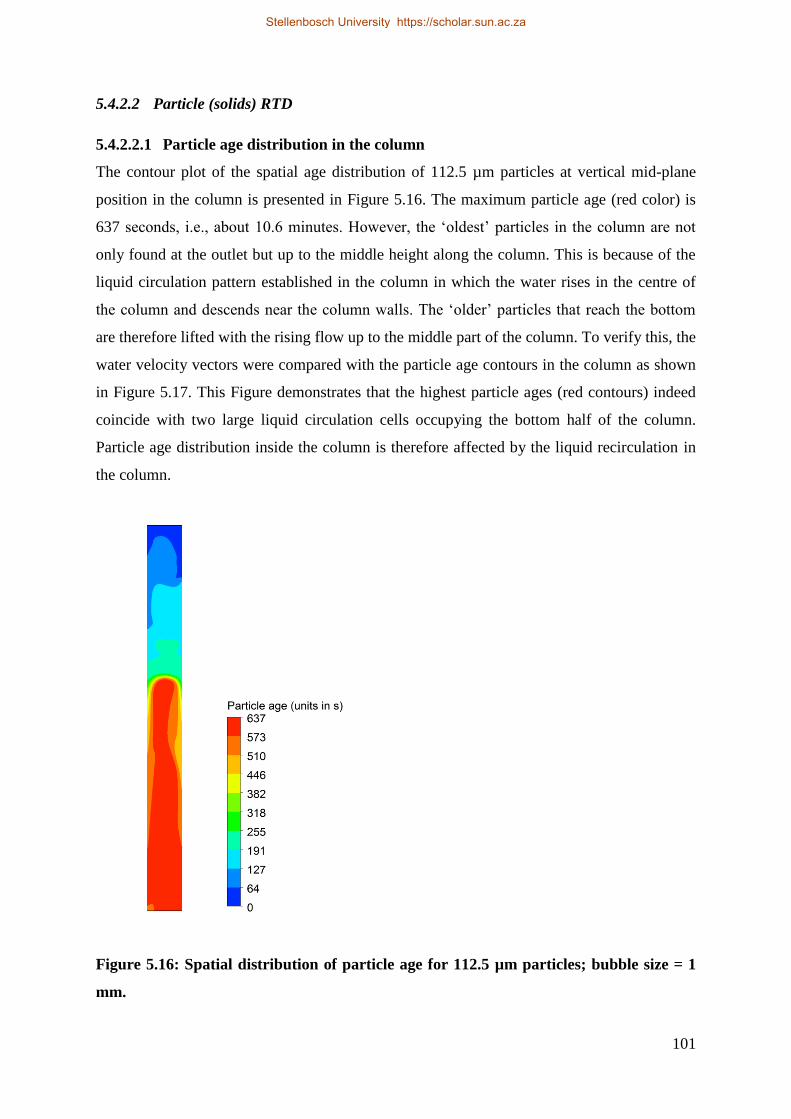
101
5.4.2.2 Particle (solids) RTD
5.4.2.2.1 Particle age distribution in the column
The contour plot of the spatial age distribution of 112.5 µm particles at vertical mid-plane
position in the column is presented in Figure 5.16. The maximum particle age (red color) is
637 seconds, i.e., about 10.6 minutes. However, the ‘oldest’ particles in the column are not
only found at the outlet but up to the middle height along the column. This is because of the
liquid circulation pattern established in the column in which the water rises in the centre of
the column and descends near the column walls. The ‘older’ particles that reach the bottom
are therefore lifted with the rising flow up to the middle part of the column. To verify this, the
water velocity vectors were compared with the particle age contours in the column as shown
in Figure 5.17. This Figure demonstrates that the highest particle ages (red contours) indeed
coincide with two large liquid circulation cells occupying the bottom half of the column.
Particle age distribution inside the column is therefore affected by the liquid recirculation in
the column.
Figure 5.16: Spatial distribution of particle age for 112.5 µm particles; bubble size = 1
mm.
Stellenbosch University https://scholar.sun.ac.za

102
Figure 5.17: Comparison of water velocity vectors with particle age contours in the
column.
5.4.2.3 Comparison of liquid and solids flow patterns at higher solids content (16.2 wt%
solids)
One of the arguments against the assumption of equal liquid and solids dispersion
coefficients is that the solids content (3 wt %) that was used in the research that led to that
conclusion [58] was too small to highlight any differences between the two phases [61].
Liquid (water) and solids axial velocity profiles obtained from CFD simulations for the 0.91
m diameter column operating with higher solids content (16.2 wt % solids) [65] were
therefore compared in order to determine whether their axial dispersion coefficients would
still be equal. The liquid and solids (56.5 and 112.5 µm) axial velocity profiles at mid-height
location are presented in Figure 5.18 and Figure 5.19. It can be seen that the solids axial
velocities are similar to the liquid ones even for the 112.5 µm particle size. The assumption
of equal solids and liquid dispersion would therefore be applicable for the operating
conditions in this column. Yianatos and Bergh [65] also reported similar conclusions from
their experimental RTD measurements.
Stellenbosch University https://scholar.sun.ac.za
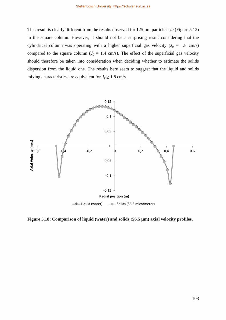
103
This result is clearly different from the results observed for 125 µm particle size (Figure 5.12)
in the square column. However, it should not be a surprising result considering that the
cylindrical column was operating with a higher superficial gas velocity (Jg = 1.8 cm/s)
compared to the square column (Jg = 1.4 cm/s). The effect of the superficial gas velocity
should therefore be taken into consideration when deciding whether to estimate the solids
dispersion from the liquid one. The results here seem to suggest that the liquid and solids
mixing characteristics are equivalent for Jg ≥ 1.8 cm/s.
Figure 5.18: Comparison of liquid (water) and solids (56.5 µm) axial velocity profiles.
-0,15
-0,1
-0,05
0
0,05
0,1
0,15
-0,6 -0,4 -0,2 0 0,2 0,4 0,6
Axi
al V
elo
city
(m
/s)
Radial position (m)
Liquid (water) Solids (56.5 micrometer)
Stellenbosch University https://scholar.sun.ac.za
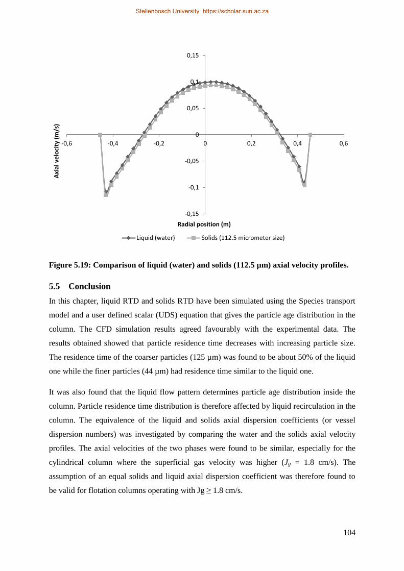
104
Figure 5.19: Comparison of liquid (water) and solids (112.5 µm) axial velocity profiles.
5.5 Conclusion
In this chapter, liquid RTD and solids RTD have been simulated using the Species transport
model and a user defined scalar (UDS) equation that gives the particle age distribution in the
column. The CFD simulation results agreed favourably with the experimental data. The
results obtained showed that particle residence time decreases with increasing particle size.
The residence time of the coarser particles (125 µm) was found to be about 50% of the liquid
one while the finer particles (44 µm) had residence time similar to the liquid one.
It was also found that the liquid flow pattern determines particle age distribution inside the
column. Particle residence time distribution is therefore affected by liquid recirculation in the
column. The equivalence of the liquid and solids axial dispersion coefficients (or vessel
dispersion numbers) was investigated by comparing the water and the solids axial velocity
profiles. The axial velocities of the two phases were found to be similar, especially for the
cylindrical column where the superficial gas velocity was higher (Jg = 1.8 cm/s). The
assumption of an equal solids and liquid axial dispersion coefficient was therefore found to
be valid for flotation columns operating with Jg ≥ 1.8 cm/s.
-0,15
-0,1
-0,05
0
0,05
0,1
0,15
-0,6 -0,4 -0,2 0 0,2 0,4 0,6
Axi
al v
elo
city
(m
/s)
Radial position (m)
Liquid (water) Solids (112.5 micrometer size)
Stellenbosch University https://scholar.sun.ac.za
105
In addition, the effects of the bubble size and particle size of the solids on the liquid
dispersion were investigated. It was found that increasing particle size of the solids resulted
in a decrease in the liquid vessel dispersion number. On the other hand, a decrease in the
bubble size caused a significant increase in the liquid vessel dispersion number.
Stellenbosch University https://scholar.sun.ac.za

106
Chapter 6 Investigation of flow regime transition in a column flotation
cell using CFD
6.1 Introduction
The focus of this chapter is to apply CFD to investigate flow regime transition in a column
flotation cell. Two types of flow characteristics can be distinguished in gas-liquid flows in
bubble columns, bubbly flow and churn-turbulent flow. The bubbly flow regime is
characterized by uniform flow of bubbles of uniform size. On the other hand, churn-turbulent
flow is characterized by a wide variation in bubble sizes with large bubbles rising rapidly and
causing liquid circulation.
Flotation columns are normally operated in the bubbly flow regime which is the optimal
condition for column flotation [2, 7, 8]. However, it has been generally observed that
flotation column performance deteriorates when the superficial gas velocity is increased
beyond a certain limit [20]. The identification of this critical or maximum superficial gas
velocity is therefore important for optimal operation of flotation columns.
Xu et al. [19, 20] investigated three phenomena that can be used to identify the maximum
superficial gas velocity in column flotation: loss of interface, loss of positive bias flow, and
loss of bubbly flow. The loss of interface occurs when the hydrodynamic conditions in the
froth zone of the column become identical to the conditions prevailing in the collection zone.
This will result in the loss of the cleaning action associated with the froth zone.
In column flotation, wash water which is continuously added at the top of the column
maintains a net downward flow of water that prevents entrained particles from reaching the
concentrate. This net downward flow of water is referred to as positive bias flow. By
minimizing entrainment of unwanted particles, a positive bias maximizes concentrate grade.
Loss of positive bias occurs when the superficial gas velocity is high enough to cause the
reversal of the net flow of water at the froth/collection zone interface.
On the other hand, the loss of bubbly flow occurs when the superficial gas velocity is
sufficiently high to bring a transition from bubbly flow conditions into churn-turbulent flow.
The increased mixing associated with churn-turbulent flow is unfavorable to the mineral
recovery in the column.
Stellenbosch University https://scholar.sun.ac.za

107
Considering the froth and liquid (pulp) phases as distinct flow regimes with different liquid
holdups, Langberg and Jameson [21] investigated the hydrodynamic conditions under which
the froth and pulp phases can coexist in a flotation cell. The effects of superficial gas velocity
and bubble size on the limiting conditions for flow regime coexistence and for countercurrent
flow across the froth-liquid interface were studied using a one dimensional two-phase flow
model. Their study identified two hydrodynamic limiting conditions relevant to the operation
of flotation cells and columns, the limiting condition for the coexistence of the froth and
liquid (pulp) phases, and the limiting condition for countercurrent flow.
Of the three phenomena used to identify the maximum superficial gas velocity in column
flotation, the loss of bubbly flow is the most difficult to determine [19, 20]. The relationship
between gas holdup and superficial gas velocity is used to determine the loss of bubbly flow
in the column. In this method, a linear gas holdup versus superficial gas velocity relationship
represents bubbly flow while deviation from linearity defines loss of bubbly flow. However,
the loss of bubbly flow is difficult to identify with this method because of the gradual nature
of the transition from bubbly flow to churn-turbulent conditions in the presence of frother
[19].
In this research, the maximum superficial gas velocity for transition from bubbly flow to
churn-turbulent flow was studied using Computational Fluid Dynamics (CFD). Besides the
gas holdup versus superficial gas velocity relationship, two alternative methods of flow
regime characterization are employed to identify the loss of bubbly flow in a pilot scale
column flotation cell. The first method involves examining the evolution of radial gas holdup
profiles as a function of superficial gas velocity. The shape of the radial gas holdup profile
has been recognized as a function of the flow pattern in two phase flows [46, 116]. On the
other hand, a graph of gas holdup versus time can also be used to identify the prevailing flow
regime in the flotation column [117]. Wide variations in the gas holdup versus time graph
characterize churn-turbulent flow conditions while gas holdup is almost constant under
bubbly flow conditions.
6.2 Methods for flow regime identification
The relationship between gas holdup and superficial gas velocity can be used to define the
prevailing flow regime in the flotation column [118]. In the bubbly flow regime, the gas
holdup increases linearly with increasing superficial gas velocity. However, the gas holdup
deviates from this linear relationship when the superficial gas velocity is increased above a
Stellenbosch University https://scholar.sun.ac.za

108
certain value as shown in Figure 6.1. The superficial gas velocity at which deviation from the
linear relationship occurs is thus the maximum or critical velocity above which the flow
regime changes from bubbly flow to churn-turbulent flow. In other words, it is the maximum
superficial gas velocity for loss of bubbly flow.
Figure 6.1: Gas holdup as a function of superficial gas velocity (adapted from Finch and
Dobby[2]).
Xu et al. [19] applied the gas holdup versus superficial gas velocity relationship to determine
the maximum superficial gas velocity for loss of bubbly flow in a pilot scale flotation
column. However, these authors reported difficulties in the identification of the regime
transition point as a result of the gradual nature of this transition particularly in the presence
of frother. The present study therefore applies the following alternative methods to
distinguish the different flow regimes and thus identify the maximum velocity above which
the transition from bubbly flow to churn-turbulent flow will occur.
6.2.1 Radial Gas Holdup profiles
Two general gas holdup profiles are known to exist, the parabolic profile and the saddle-
shaped profile. Kobayasi et al. [116] studied the characteristics of the local void fraction (gas
holdup) distribution in air-water two phase flow. They reported a ‘peculiar’ distribution,
Bubbly flow
regime
Churn-turbulent flow
regime
Transition
Superficial gas velocity (cm/s)
Gas
hold
up
, (%
)
Stellenbosch University https://scholar.sun.ac.za
109
different from the previously accepted power law distribution in bubbly flow conditions. The
distribution associated with bubbly flow has its peaks near the pipe wall. On the other hand,
the distribution in slug flow had its maximum at the centre of the pipe.
Serizawa et al. [46] also studied various local parameters and turbulence characteristics of
concurrent air-water two phase bubbly flow. They found that the distribution of void fraction
(radial gas holdup) was a strong function of the flow pattern. The void fraction distribution
changed from saddle shaped to parabolic as gas velocity increased. A saddle shaped
distribution is therefore associated with bubbly flow conditions, while a parabolic one
represents slug flow.
6.2.2 Gas holdup versus Time graph
A plot of gas holdup versus time can also be used to identify the existing flow regime in a
column The gas holdup versus time will be relatively constant when the column is in the
bubbly flow regime. On the other hand, the gas holdup will show wide variations when the
column is operating in the churn-turbulent regime.[117]. A similar method has been used by
previous researchers in which variations in conductivity signals were used to characterize the
flow regime in the downcomer of a Jameson flotation cell [119, 120].
6.3 Description of the modeled column
The CFD model developed in the present research was used to simulate the flotation column
that was used in the experimental work of Xu et al. [19, 20]. The column was made of
Plexiglas and was 400 cm in height and 10.16 cm in diameter. The column was operated
continuously and air was introduced into the bottom of the column through a cylindrical
stainless steel sparger, 3.8 cm in diameter and 7 cm in length. This sparger geometry gives a
ratio of column cross-section to sparger surface area of about 1:1. A schematic diagram of the
column is presented in Figure 6.2. A detailed description of the experimental set up is
presented elsewhere [20].
Stellenbosch University https://scholar.sun.ac.za
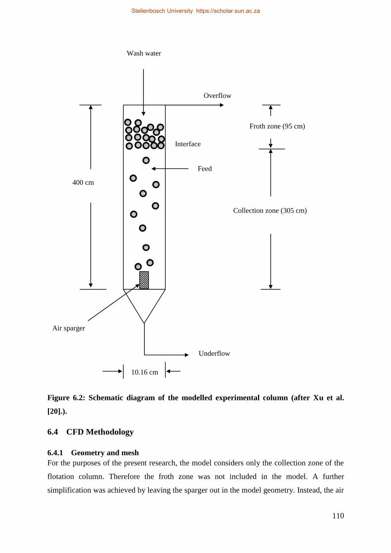
110
Figure 6.2: Schematic diagram of the modelled experimental column (after Xu et al.
[20].).
6.4 CFD Methodology
6.4.1 Geometry and mesh
For the purposes of the present research, the model considers only the collection zone of the
flotation column. Therefore the froth zone was not included in the model. A further
simplification was achieved by leaving the sparger out in the model geometry. Instead, the air
Underflow
Overflow
10.16 cm
Air sparger
Froth zone (95 cm)
400 cm
Interface
Wash water
Feed
Collection zone (305 cm)
Stellenbosch University https://scholar.sun.ac.za

111
was introduced from the bottom part of the column over the entire column cross section. This
will not affect the required gas holdup prediction since the ratio of column cross-section to
sparger surface area was about 1:1 in the experimental flotation column. The result of these
simplifications is that the model geometry is reduced to a cylindrical vessel of height equal to
the collection zone height (305 cm in this case) and diameter equal to the diameter of the
experimental flotation column.
A mesh comprising mainly hexahedral elements was generated over the model geometry
using the sweep method in ANSYS Meshing. Five mesh sizes were investigated in order to
achieve grid independent numerical results. The mesh sizes are summarized in Table 6.1
together with their respective attributes.
Table 6.1: The five mesh sizes and their respective characteristics.
Mesh Number of cells Number of nodes Minimum
Orthogonal
Quality
CPU time (Hrs)
Mesh 1 13,940 17,510 0.9318 2.5
Mesh 2 34,160 39,474 0.939 4.5
Mesh 3 79,755 88,560 0.773 14
Mesh 4 98,112 108,433 0.831 16
Mesh 5 114,696 126,764 0.878 17
The axial water and bubble velocity profiles obtained for the different mesh sizes are shown
in Figure 6.3 and Figure 6.4, respectively. Grid independence was achieved with mesh 3 to
mesh 4 and 5. Mesh 3 (79,755 elements) was therefore selected for all subsequent simulations
in this study.
Stellenbosch University https://scholar.sun.ac.za

112
Figure 6.3: Water velocity profiles at mid-height in the collection zone (Height = 152.5
cm).
Figure 6.4: Bubble velocity profiles at mid-height in the collection zone (Height = 152.5
cm).
-0,15
-0,1
-0,05
0
0,05
0,1
0,15
0,2
-0,06 -0,04 -0,02 0 0,02 0,04 0,06
Me
an A
xial
wat
er
velo
city
(m
/s)
Radial position (m)
Mesh 1 Mesh 2 Mesh 3 Mesh 4 Mesh 5
0
0,05
0,1
0,15
0,2
0,25
0,3
0,35
-0,06 -0,04 -0,02 0 0,02 0,04 0,06
Bu
bb
le v
elo
city
(m
/s)
Radial position (m)
Mesh 1 Mesh 2 Mesh 3 Mesh 4 Mesh 5
Stellenbosch University https://scholar.sun.ac.za
113
6.4.2 Boundary conditions
Air bubbles were introduced into the column through mass and momentum source terms at
the column bottom. The source terms were calculated from the respective superficial gas
velocities and were applied over the entire column cross section at the bottom (source) and at
the top (sink) of the collection zone.
For the liquid phase, the top of the collection zone was modelled as a velocity inlet boundary
where inlet velocity was specified as equal to superficial liquid velocity Jl. Since the
computational domain being considered is the collection zone of the column, the superficial
liquid velocity must include the feed rate plus the bias water resulting from wash water
addition. The superficial liquid velocity is therefore equal to the superficial tailing rate, Jt.
The bottom part was also modelled as velocity inlet where exit velocity was set equal to
minus superficial liquid velocity. At the column wall, no slip boundary conditions were
applied for both the air bubbles and the liquid phase.
6.4.3 Multiphase Model
The Eulerian-Eulerian (E-E) multiphase modelling approach used in this study has already
been described in Chapter 3. Interaction between the phases in the model was accounted for
through inclusion of the drag force between phases. The drag force is included in the
respective momentum conservation equations as a source term. The continuity and
momentum equations for the Eulerian-Eulerian model have been presented in Chapter 3 in
equations (3.3) and (3.4) and will not be repeated here for brevity. The volume fraction (or
gas holdup) of the secondary phase was calculated from the mass conservation equations as
described in section 4.3.3 using equation (4.2).
In the present study, the drag coefficient was calculated using the universal drag laws [94]. In
this case, the drag coefficient is defined in different ways depending on whether the
prevailing regime is in the viscous regime category, the distorted bubble regime, or the
strongly deformed capped bubbles regime. The different regimes are defined on the basis of
the Reynolds number. In the viscous regime the drag coefficient is presented as:
𝐶𝐷𝑣𝑖𝑠
=24
𝑅𝑒(1 + 0.1𝑅𝑒0.75) (6.1)
where Re is the relative Reynolds number for the primary phase L and the secondary phase G
defined as:
Stellenbosch University https://scholar.sun.ac.za

114
𝑅𝑒 =
𝜌𝐿|𝒖𝐿⃗⃗ ⃗⃗ − 𝒖𝐺⃗⃗⃗⃗ ⃗|𝑑𝐵
𝜇𝑒 (6.2)
and µe is the effective viscosity for the bubble-liquid mixture given by:
𝜇𝑒 =𝜇𝐿
1 − 휀𝐺 (6.3)
In the distorted bubble regime the drag coefficient is given as follows:
𝐶𝐷𝑑𝑖𝑠= 2 3⁄ (
𝑑𝐵
𝜆𝑅𝑇) {
1 + 17.67𝑓6
7⁄
18.67𝑓}
2
; 𝑓 = (1 − 휀𝐺)1.5 (6.4)
where λRT is the Rayleigh-Taylor instability wavelength defined as follows:
𝜆𝑅𝑇 = (
𝜎
𝑔∆𝜌𝐺𝐿)0.5
(6.5)
and σ is the surface tension, g the gravitational acceleration, and ΔρGL is the absolute value of
the density difference between the phases G and L.
For the strongly deformed, capped bubbles regime, the following drag coefficient is used:
𝐶𝐷𝑐𝑎𝑝
=8
3(1 − 휀𝐺)2 (6.6)
Under churn-turbulent flow conditions, the drag coefficient is calculated using equation(6.6).
Further details about the universal drag laws are available in a recent multiphase flow
dynamics book [94].
6.4.4 Turbulence Modeling
Turbulence in the continuous phase was modelled using the k-ϵ realizable turbulence model,
a RANS (Reynolds- Averaged Navier- Stokes) based model in which the time averaged
Navier-Stokes (RANS) equations are solved in place of the instantaneous Navier-Stokes
equations to produce a time averaged flow field. The averaging procedure introduces
additional unknown terms; the Reynolds stresses which are subsequently resolved by
employing Boussinesq’s eddy viscosity concept where the Reynolds stresses (or turbulent
stresses) are related to the velocity gradients according to equation (3.9) as described in
section 3.4.3 where the realizaable k-e model is explained.
Stellenbosch University https://scholar.sun.ac.za
115
6.4.5 Numerical solution methods
The momentum and volume fraction equations were discretized using the first order upwind
scheme. The first order upwind scheme was also employed for turbulence kinetic energy and
dissipation rate discretization. A time step size of 0.05s was used in all the simulations. The
simulations were run up to a flow time of at least 240s. Time averaging was carried out over
the last 120s.
6.5 Results and discussion
If the entire range of bubble sizes encompassing the different flow regimes is known, CFD
simulations can be conducted for a range of superficial gas velocities covering the different
flow regimes. A plot of gas holdup versus superficial gas velocity can then be used to
determine the point of departure from bubbly flow conditions as described earlier. For a
system comprising of water and air without frother, an empirical formula derived by Shen
[117] can be used to calculate the Sauter mean bubble size as a function of the superficial gas
velocity. However, a similar empirical equation derived for column flotation conditions
where frother plays an important role in determining the bubble size is only limited to
superficial gas velocities ranging from 1 to 3 cm/s. The first set of CFD results presented in
this study is therefore obtained using bubble sizes calculated for a system without frother.
The gas holdup versus superficial gas velocity relationship obtained is then used to delineate
the different flow regimes prevailing in the column.
Once the flow regimes are identified, the evolution of radial gas holdup profiles and gas
holdup versus time graphs can be examined for the flow regimes determined from the gas
holdup versus superficial gas velocity graph. Radial gas holdup profiles and gas holdup
versus. time graphs are then used to determine the maximum superficial gas velocity for a
column operating with an average bubble size of 1.5 mm which is comparable with typical
bubble sizes being used in industrial flotation columns. The radial gas holdup profiles were
obtained at the mid-height position (152.5 cm height) in the column. On the other hand, the
gas holdup versus time graphs were obtained from a surface monitor located at column mid-
height position from which area weighted average gas holdup measurements were recorded at
5 second intervals.
It is important at this stage, to clarify the definition of regime transition and churn-turbulent
flow regime as used in the present study. Churn-turbulent flow is normally associated with a
wide bubble size distribution including large bubbles. However, the CFD simulations in the
Stellenbosch University https://scholar.sun.ac.za
116
present research were conducted with a single mean bubble size assigned for each superficial
gas velocity. Furthermore, in order to investigate the flow regime transition for conditions
relevant to column flotation, the other set of CFD simulations was performed with the bubble
size held at a constant value of 1.5 mm while increasing the superficial gas velocity to
determine the maximum superficial gas velocity for that particular bubble size. The reference
to churn-turbulent flow in the present study is therefore not based on a wide bubble size
distribution of large bubbles in the presence of smaller ones. On the other hand, a CFD model
coupled with a bubble population balance model can be used to predict bubble size
distributions in the column. However, the present research did not incorporate bubble
population balance modelling.
According to Lockett and Kirkpatrick [121] there are three main reasons for breakaway from
ideal bubbly flow; flooding, liquid circulation, and the presence of large bubbles. It should
therefore be possible to identify regime transition from changes in the pattern and intensity of
the liquid circulation in the column even if changes in bubble size are negligible or absent.
On the other hand, the liquid circulation pattern and its intensity depend on the prevailing
radial gas holdup profile in the column [48].
Saddle shaped gas holdup profiles have already been related to bubbly flow conditions in
two-phase flows [46, 116]. However, the bubbly flow regime is generally characterized by a
radially uniform gas holdup distribution [122-124]. Both saddle and flat gas holdup profiles
can therefore be considered to indicate the existence of the bubbly flow regime in the column.
On the other hand, the churn-turbulent flow regime is generally distinguished by a non-
uniform radial gas holdup distribution causing bulk liquid circulation. Parabolic gas holdup
profiles are therefore interpreted to signify churn-turbulent flow conditions in the column.
6.5.1 Water and air only (without frother)
For the water and air only (no frother) system, CFD simulations were carried out for
superficial gas velocities ranging from 1.01 to 14 cm/s to encompass both the bubbly flow
and churn-turbulent flow regimes. The Sauter mean bubble size for a multi-bubble system
without frother (i.e., water and air only) can be calculated as a function of the superficial gas
velocities from the following empirical formula [117]:
𝑑𝐵𝑆 = 0.33(𝐽𝑔)0.24
(6.7)
Stellenbosch University https://scholar.sun.ac.za
117
This empirical formula was derived for a laboratory flotation column with a porous stainless
steel sparger similar to the one that was used in the column being modelled in the present
work. The equation was therefore used in the present work to calculate the average bubble
sizes that were subsequently used in the CFD simulations.
6.5.1.1 Gas holdup versus superficial gas velocity (gas rate) graph
The graph of gas holdup versus superficial gas velocity obtained from CFD simulations is
presented in Figure 6.5. The different flow regimes can be cleared delineated as follows:
Bubbly flow regime; Jg 1.01 – 6.12 cm/s (linear portion of the graph)
Transition; 6.12 < Jg ≤ 11.71 cm/s (deviation from linear relationship between gas
holdup and superficial gas velocity)
Churn-turbulent flow; Jg > 11.71 cm/s (third portion of the gas holdup versus
superficial gas velocity graph)
The maximum superficial gas velocity (Jgmax) before loss of bubbly flow is therefore equal
to 6.12 cm/s for the water and air only system (without frother). This value compares well
with the maximum superficial gas velocity of 5.25 cm/s for loss of bubbly flow predicted
from drift flux theory by Xu et al. [20].
Having delineated the different flow regimes using the gas holdup versus superficial gas
velocity relationship, the evolution of the radial gas holdup profiles was examined as the
superficial gas velocity increased from 1.01 cm/s to 14 cm/s.
Stellenbosch University https://scholar.sun.ac.za
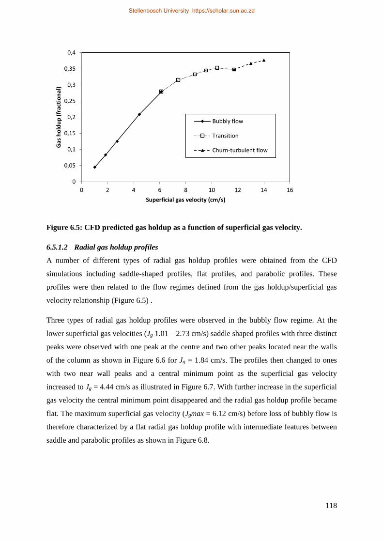
118
Figure 6.5: CFD predicted gas holdup as a function of superficial gas velocity.
6.5.1.2 Radial gas holdup profiles
A number of different types of radial gas holdup profiles were obtained from the CFD
simulations including saddle-shaped profiles, flat profiles, and parabolic profiles. These
profiles were then related to the flow regimes defined from the gas holdup/superficial gas
velocity relationship (Figure 6.5) .
Three types of radial gas holdup profiles were observed in the bubbly flow regime. At the
lower superficial gas velocities (Jg 1.01 – 2.73 cm/s) saddle shaped profiles with three distinct
peaks were observed with one peak at the centre and two other peaks located near the walls
of the column as shown in Figure 6.6 for Jg = 1.84 cm/s. The profiles then changed to ones
with two near wall peaks and a central minimum point as the superficial gas velocity
increased to Jg = 4.44 cm/s as illustrated in Figure 6.7. With further increase in the superficial
gas velocity the central minimum point disappeared and the radial gas holdup profile became
flat. The maximum superficial gas velocity (Jgmax = 6.12 cm/s) before loss of bubbly flow is
therefore characterized by a flat radial gas holdup profile with intermediate features between
saddle and parabolic profiles as shown in Figure 6.8.
0
0,05
0,1
0,15
0,2
0,25
0,3
0,35
0,4
0 2 4 6 8 10 12 14 16
Gas
ho
ldu
p (
frac
tio
nal
)
Superficial gas velocity (cm/s)
Bubbly flow
Transition
Churn-turbulent flow
Stellenbosch University https://scholar.sun.ac.za
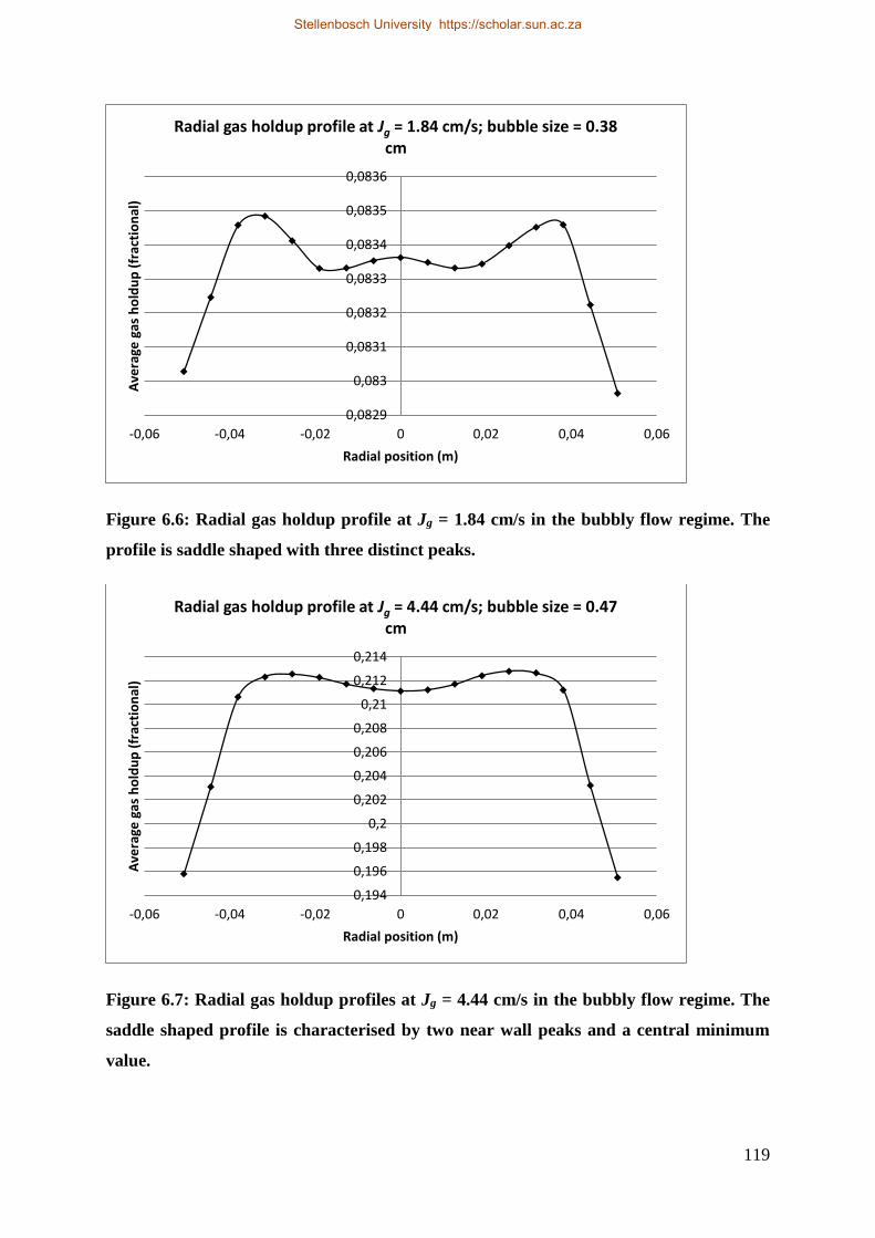
119
Figure 6.6: Radial gas holdup profile at Jg = 1.84 cm/s in the bubbly flow regime. The
profile is saddle shaped with three distinct peaks.
Figure 6.7: Radial gas holdup profiles at Jg = 4.44 cm/s in the bubbly flow regime. The
saddle shaped profile is characterised by two near wall peaks and a central minimum
value.
0,0829
0,083
0,0831
0,0832
0,0833
0,0834
0,0835
0,0836
-0,06 -0,04 -0,02 0 0,02 0,04 0,06
Ave
rage
gas
ho
ldu
p (
frac
tio
nal
)
Radial position (m)
Radial gas holdup profile at Jg = 1.84 cm/s; bubble size = 0.38 cm
0,194
0,196
0,198
0,2
0,202
0,204
0,206
0,208
0,21
0,212
0,214
-0,06 -0,04 -0,02 0 0,02 0,04 0,06
Ave
rage
gas
ho
ldu
p (
frac
tio
nal
)
Radial position (m)
Radial gas holdup profile at Jg = 4.44 cm/s; bubble size = 0.47 cm
Stellenbosch University https://scholar.sun.ac.za

120
Figure 6.8: Radial gas holdup profile at Jg = 6.12 cm/s (Jgmax) showing a flat profile
with features intermediate between saddle and parabolic profiles.
The transition from bubbly flow to churn-turbulent flow was gradual and characterized by
flat (Jg = 7.41 cm/s) to parabolic (Jg 8.70 – 11.71 cm/s) radial gas holdup profiles. The
parabolic profiles became progressively steep as the superficial gas velocity increased.
Eventually the flow regime changes into churn-turbulent flow (Jg > 11.71 cm/s) which is
characterized by steep parabolic gas holdup profiles as shown in Figure 6.9.
6.5.1.3 Gas holdup versus time graphs
Another method that was used to distinguish flow regimes in the water–air system using CFD
simulations was by means of gas holdup versus time graphs. Comparing the two extreme
cases, the gas holdup versus time was mostly constant in the bubbly flow regime as shown in
Figure 6.10 for Jg = 1.84 cm/s, except for moderate variations at the maximum superficial gas
velocity. On the hand hand, very wide variations in gas holdup were observed in the churn-
turbulent flow regime (i.e., Jg > 11.71 cm/s), as illustrated in Figure 6.11 for Jg = 14 cm/s.
The transition from bubbly flow to churn-turbulent flow pattern was gradual and
characterized by moderate to large fluctuations in gas holdup in which the gas holdup
variations became increasingly intense as the superficial gas velocity increased.
0,26
0,265
0,27
0,275
0,28
0,285
0,29
-0,06 -0,04 -0,02 0 0,02 0,04 0,06
Ave
rage
gas
ho
ldu
p (
frac
tio
nal
)
Radial position (m)
Radial gas holdup profile at Jg = 6.12 cm/s; bubble size = 0.51 cm
Stellenbosch University https://scholar.sun.ac.za

121
Figure 6.9: Radial gas holdup profile at Jg = 14 cm/s in the churn-turbulent flow regime.
The typical profile is a steep parabolic profile.
Figure 6.10: Gas holdup versus time graph for Jg = 1.84 cm/s. The constant gas holdup
indicates bubbly flow conditions in the column.
0,25
0,3
0,35
0,4
0,45
0,5
-0,06 -0,04 -0,02 0 0,02 0,04 0,06
Ave
rage
gas
ho
ldu
p (
frac
tio
nal
)
Radial position (m)
Radial gas holdup profile at Jg = 14.00 cm/s; bubble size = 0.62 cm
0
0,02
0,04
0,06
0,08
0,1
0,12
0,14
0,16
0 50 100 150 200
Ave
rage
gas
ho
ldu
p (
frac
tio
nal
)
Time (Seconds)
Stellenbosch University https://scholar.sun.ac.za

122
Figure 6.11: Gas holdup versus time graph for Jg = 14 cm/s. The wide variations in gas
holdup are a characteristic feature of the churn-turbulent flow regime.
The results from the CFD simulations of the water and air only (no frother) system where
bubble sizes are calculated from the superficial gas velocity according to equation (6.7) are
summarized in Table 6.2. The progression from bubbly flow conditions to churn-turbulent
flow can also be clearly appreciated from this Table. The distinguishing characteristics of the
flow regimes are summarised in Table 6.3.
0,25
0,27
0,29
0,31
0,33
0,35
0,37
0,39
0,41
0 50 100 150 200
Ave
rage
gas
ho
ldu
p (
frac
tio
nal
)
Time (Seconds)
Stellenbosch University https://scholar.sun.ac.za
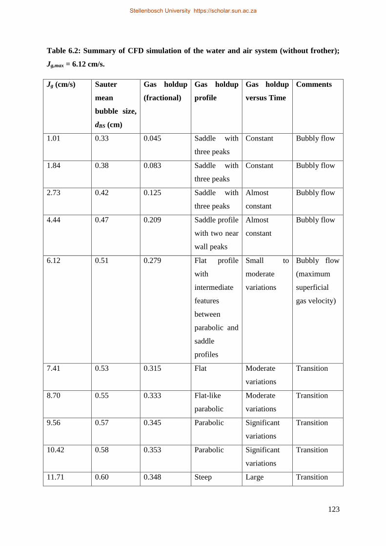
123
Table 6.2: Summary of CFD simulation of the water and air system (without frother);
Jg,max = 6.12 cm/s.
Jg (cm/s) Sauter
mean
bubble size,
dBS (cm)
Gas holdup
(fractional)
Gas holdup
profile
Gas holdup
versus Time
Comments
1.01 0.33 0.045 Saddle with
three peaks
Constant Bubbly flow
1.84 0.38 0.083 Saddle with
three peaks
Constant Bubbly flow
2.73 0.42 0.125 Saddle with
three peaks
Almost
constant
Bubbly flow
4.44 0.47 0.209 Saddle profile
with two near
wall peaks
Almost
constant
Bubbly flow
6.12 0.51 0.279 Flat profile
with
intermediate
features
between
parabolic and
saddle
profiles
Small to
moderate
variations
Bubbly flow
(maximum
superficial
gas velocity)
7.41 0.53 0.315 Flat Moderate
variations
Transition
8.70 0.55 0.333 Flat-like
parabolic
Moderate
variations
Transition
9.56 0.57 0.345 Parabolic Significant
variations
Transition
10.42 0.58 0.353 Parabolic Significant
variations
Transition
11.71 0.60 0.348 Steep Large Transition
Stellenbosch University https://scholar.sun.ac.za
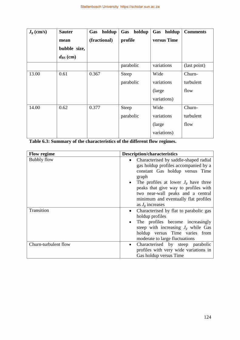
124
Jg (cm/s) Sauter
mean
bubble size,
dBS (cm)
Gas holdup
(fractional)
Gas holdup
profile
Gas holdup
versus Time
Comments
parabolic variations (last point)
13.00 0.61 0.367 Steep
parabolic
Wide
variations
(large
variations)
Churn-
turbulent
flow
14.00 0.62 0.377 Steep
parabolic
Wide
variations
(large
variations)
Churn-
turbulent
flow
Table 6.3: Summary of the characteristics of the different flow regimes.
Flow regime Description/characteristics
Bubbly flow Characterised by saddle-shaped radial
gas holdup profiles accompanied by a
constant Gas holdup versus Time
graph
The profiles at lower Jg have three
peaks that give way to profiles with
two near-wall peaks and a central
minimum and eventually flat profiles
as Jg increases
Transition Characterised by flat to parabolic gas
holdup profiles
The profiles become increasingly
steep with increasing Jg while Gas
holdup versus Time varies from
moderate to large fluctuations
Churn-turbulent flow Characterised by steep parabolic
profiles with very wide variations in
Gas holdup versus Time
Stellenbosch University https://scholar.sun.ac.za

125
6.5.2 Water with frother (as in column flotation)
In flotation columns, the bubble size depends not only on the superficial gas velocity but also
on other physical chemical characteristics of the gas-liquid system. In this case, the bubble
size can be calculated as a function of the superficial gas velocity according to the following
relationship [2, 8].
𝑑𝐵 = 𝐶(𝐽𝑔)𝑛
(6.8)
where C and n are constants. The constant C is a fitting parameter which depends mainly on
frother concentration, the sparger size and column size. Simulations were carried out for the
experimental conditions used by Xu et al. [19, 20] particularly the case in which the frother
concentration was 10 ppm. The value of C was therefore equal to 1 while n was 0.25.
The gas holdup obtained from the CFD simulations is plotted as a function of superficial gas
velocity in Figure 6.12. The experimental data from Xu et al. [19] are included in the Figure
for comparison. It can be seen that the predicted gas holdup is in good agreement with the
experimental data up to superficial gas velocity Jg = 3.60 cm/s. Above Jg = 3.60 cm/s, the
relationship in equation (6.8) is not applicable because the value of the exponent n (0.25) is
valid for Jg 1 – 3 cm/s [8]. Unfortunately there is no equation relating bubble size and
superficial gas velocity for flow conditions above Jg = 3 cm/s. Therefore, the gas holdup
versus superficial gas velocity graph obtained from CFD simulations cannot be used to
determine the maximum superficial gas velocity since the range of bubble sizes for the
different flow regimes cannot be completely determined.
On the other hand, Xu et al. [19] used the gas holdup versus superficial gas velocity
relationship to identify the maximum gas velocity for loss of bubbly flow. However, they
reported a gradual and unclear transition from bubbly flow to churn-turbulent flow
conditions. The maximum superficial gas velocity for conditions applicable in flotation
columns can be obtained using radial gas holdup profiles and the gas holdup versus time
graphs as already described. In this regard, CFD simulations were performed for a stipulated
bubble size of 1.5 mm which is similar to common bubble sizes used in column flotation. The
bubble size was held constant during the simulations while increasing the superficial gas
velocity to encompass both bubbly flow and churn-turbulent flow conditions.
Stellenbosch University https://scholar.sun.ac.za
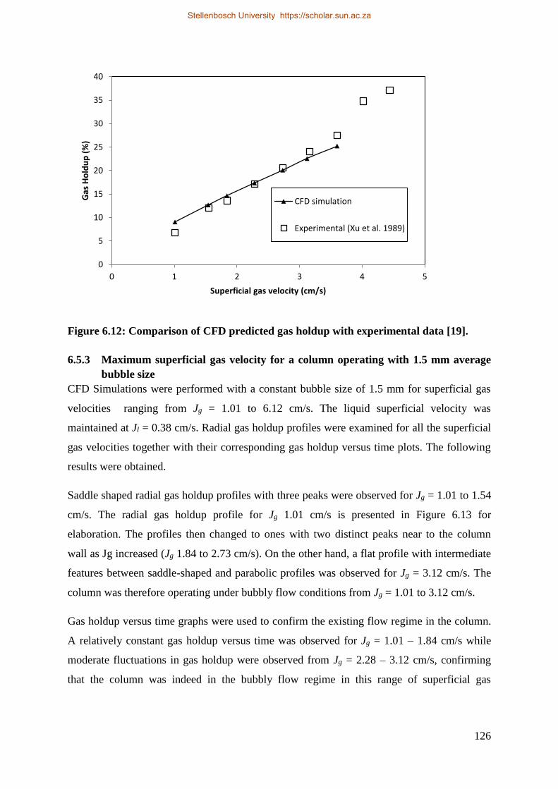
126
Figure 6.12: Comparison of CFD predicted gas holdup with experimental data [19].
6.5.3 Maximum superficial gas velocity for a column operating with 1.5 mm average
bubble size
CFD Simulations were performed with a constant bubble size of 1.5 mm for superficial gas
velocities ranging from Jg = 1.01 to 6.12 cm/s. The liquid superficial velocity was
maintained at Jl = 0.38 cm/s. Radial gas holdup profiles were examined for all the superficial
gas velocities together with their corresponding gas holdup versus time plots. The following
results were obtained.
Saddle shaped radial gas holdup profiles with three peaks were observed for Jg = 1.01 to 1.54
cm/s. The radial gas holdup profile for Jg 1.01 cm/s is presented in Figure 6.13 for
elaboration. The profiles then changed to ones with two distinct peaks near to the column
wall as Jg increased (Jg 1.84 to 2.73 cm/s). On the other hand, a flat profile with intermediate
features between saddle-shaped and parabolic profiles was observed for Jg = 3.12 cm/s. The
column was therefore operating under bubbly flow conditions from Jg = 1.01 to 3.12 cm/s.
Gas holdup versus time graphs were used to confirm the existing flow regime in the column.
A relatively constant gas holdup versus time was observed for Jg = 1.01 – 1.84 cm/s while
moderate fluctuations in gas holdup were observed from Jg = 2.28 – 3.12 cm/s, confirming
that the column was indeed in the bubbly flow regime in this range of superficial gas
0
5
10
15
20
25
30
35
40
0 1 2 3 4 5
Gas
Ho
ldu
p (
%)
Superficial gas velocity (cm/s)
CFD simulation
Experimental (Xu et al. 1989)
Stellenbosch University https://scholar.sun.ac.za
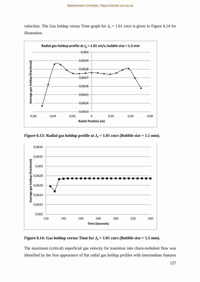
127
velocities. The Gas holdup versus Time graph for Jg = 1.01 cm/s is given in Figure 6.14 for
illustration.
Figure 6.13: Radial gas holdup profile at Jg = 1.01 cm/s (Bubble size = 1.5 mm).
Figure 6.14: Gas holdup versus Time for Jg = 1.01 cm/s (Bubble size = 1.5 mm).
The maximum (critical) superficial gas velocity for transition into churn-turbulent flow was
identified by the first appearance of flat radial gas holdup profiles with intermediate features
0,0623
0,0624
0,0625
0,0626
0,0627
0,0628
0,0629
0,063
-0,06 -0,04 -0,02 0 0,02 0,04 0,06
Ave
rage
gas
ho
ldu
p (
frac
tio
nal
)
Radial Position (m)
Radial gas holdup profile at Jg = 1.01 cm/s; bubble size = 1.5 mm
0,062
0,0622
0,0624
0,0626
0,0628
0,063
0,0632
0,0634
120 140 160 180 200 220 240
Ave
rage
gas
ho
ldu
p (
frac
tio
nal
)
Time (Seconds)
Stellenbosch University https://scholar.sun.ac.za

128
between parabolic and saddle shaped profiles at Jg = 3.12 cm/s. Thus, for a constant bubble
size of 1.5 mm the transition to churn-turbulent flow begins at Jg = 3.6 cm/s. The maximum
superficial gas velocity (Jg,max) before loss of bubbly flow is therefore 3.12 cm/s for a
flotation column operating with an average bubble size of 1.5 mm at superficial liquid
velocity (Jl) equal to 0.38 cm/s. This compares favorably with the maximum gas velocity of
3.60 cm/s reported by Xu et al. [19, 20] with reference to loss of interface. Indeed these
authors did report that loss of interface and loss of bubbly flow occurred at approximately the
same superficial gas velocities. The predicted gas holdup at Jg,max is equal to 20.1% which
compares favorably with the maximum gas holdup of 20 to 24% reported by Dobby et al.
[44].
The radial gas holdup profile at Jg,max is shown in Figure 6.15 and its corresponding Gas
holdup versus Time graph in Figure 6.16. It can be seen that the maximum superficial gas
velocity is characterized by a flat gas holdup profile accompanied by moderate gas holdup
fluctuations.
Figure 6.15: Radial gas holdup profile at Jg,max (3.12 cm/s).
0,192
0,194
0,196
0,198
0,2
0,202
0,204
-0,06 -0,04 -0,02 0 0,02 0,04 0,06
Ave
rage
gas
ho
ldu
p (
frac
tio
nal
)
Radial Position (m)
Radial gas holdup profile at Jg = 3.12 cm/s; bubble size = 1.5 mm
Stellenbosch University https://scholar.sun.ac.za

129
Figure 6.16: Gas holdup versus Time graph for Jg = 3.12 cm/s (Jg,max); bubble size = 1.5
mm.
In the churn-turbulent regime, steeper parabolic radial gas holdup profiles were observed
from Jg = 5.28 cm/s as shown in Figure 6.17. On the other hand, very wide variations in Gas
holdup versus Time at Jg = 5.28 cm/s (Figure 6.18) further confirm that the churn-turbulent
flow regime was now prevailing in the column. The results from the CFD simulations for 1.5
mm bubble size are summarized in Table 6.4. The progression from bubbly flow conditions
to churn-turbulent flow can be clearly seen in the Table.
0,185
0,19
0,195
0,2
0,205
0,21
0,215
120 140 160 180 200 220 240
Ave
rage
gas
ho
ldu
p (
frac
tio
nal
)
Time (Seconds)
Stellenbosch University https://scholar.sun.ac.za
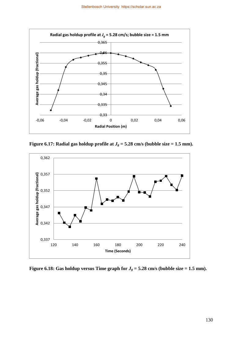
130
Figure 6.17: Radial gas holdup profile at Jg = 5.28 cm/s (bubble size = 1.5 mm).
Figure 6.18: Gas holdup versus Time graph for Jg = 5.28 cm/s (bubble size = 1.5 mm).
0,33
0,335
0,34
0,345
0,35
0,355
0,36
0,365
-0,06 -0,04 -0,02 0 0,02 0,04 0,06
Ave
rage
gas
ho
ldu
p (
frac
tio
nal
)
Radial Position (m)
Radial gas holdup profile at Jg = 5.28 cm/s; bubble size = 1.5 mm
0,337
0,342
0,347
0,352
0,357
0,362
120 140 160 180 200 220 240
Ave
rage
gas
ho
ldu
p (
frac
tio
nal
)
Time (Seconds)
Stellenbosch University https://scholar.sun.ac.za
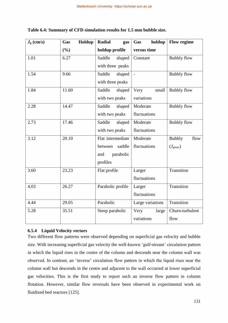
131
Table 6.4: Summary of CFD simulation results for 1.5 mm bubble size.
Jg (cm/s) Gas Holdup
(%)
Radial gas
holdup profile
Gas holdup
versus time
Flow regime
1.01 6.27 Saddle shaped
with three peaks
Constant Bubbly flow
1.54 9.66 Saddle shaped
with three peaks
- Bubbly flow
1.84 11.60 Saddle shaped
with two peaks
Very small
variations
Bubbly flow
2.28 14.47 Saddle shaped
with two peaks
Moderate
fluctuations
Bubbly flow
2.73 17.46 Saddle shaped
with two peaks
Moderate
fluctuations
Bubbly flow
3.12 20.10 Flat intermediate
between saddle
and parabolic
profiles
Moderate
fluctuations
Bubbly flow
(Jgmax)
3.60 23.23 Flat profile Larger
fluctuations
Transition
4.03 26.27 Parabolic profile Larger
fluctuations
Transition
4.44 29.05 Parabolic Large variations Transition
5.28 35.51 Steep parabolic Very large
variations
Churn-turbulent
flow
6.5.4 Liquid Velocity vectors
Two different flow patterns were observed depending on superficial gas velocity and bubble
size. With increasing superficial gas velocity the well-known ‘gulf-stream’ circulation pattern
in which the liquid rises in the centre of the column and descends near the column wall was
observed. In contrast, an ‘inverse’ circulation flow pattern in which the liquid rises near the
column wall but descends in the centre and adjacent to the wall occurred at lower superficial
gas velocities. This is the first study to report such an inverse flow pattern in column
flotation. However, similar flow reversals have been observed in experimental work on
fluidized bed reactors [125].
Stellenbosch University https://scholar.sun.ac.za

132
The inverse circulation pattern has been theoretically investigated in bubble columns and is
associated with fully developed saddle-shaped radial gas holdup profiles [51, 126]. In the
present study, the inverse circulation pattern was observed at Jg = 1.01 cm/s and Jg = 1.54
cm/s for simulations with bubble size = 1.5 mm and superficial liquid velocity = 0.38 cm/s.
Prominent saddle shaped gas holdup profiles with two distinct peaks near the walls of the
column were also present under these conditions. The liquid velocity vector plots obtained
from CFD simulations are presented in Figure 6.19 and Figure 6.20 for the two circulation
patterns.
Clark et al. [126] have described the sequence of events that may initiate liquid circulation in
bubble columns. In general, liquid circulation in bubble columns is initiated by density
differences in the gas-liquid mixture depending on the prevailing radial gas holdup profile. If
the concentration of air bubbles is higher in the central part of the column compared to the
outer annular region, the mean mixture density will be lower near the centre of the column
than in the outer annulus. The hydrostatic pressure head will therefore be higher in the outer
annulus hence a radial pressure difference is set up inside the column. This will cause an
inward radial movement of liquid and initiate liquid circulation. The inverse circulation
pattern will occur if the concentration of bubbles is higher in the outer annular region as
happens in the case of saddle-shaped gas holdup profiles.
Stellenbosch University https://scholar.sun.ac.za
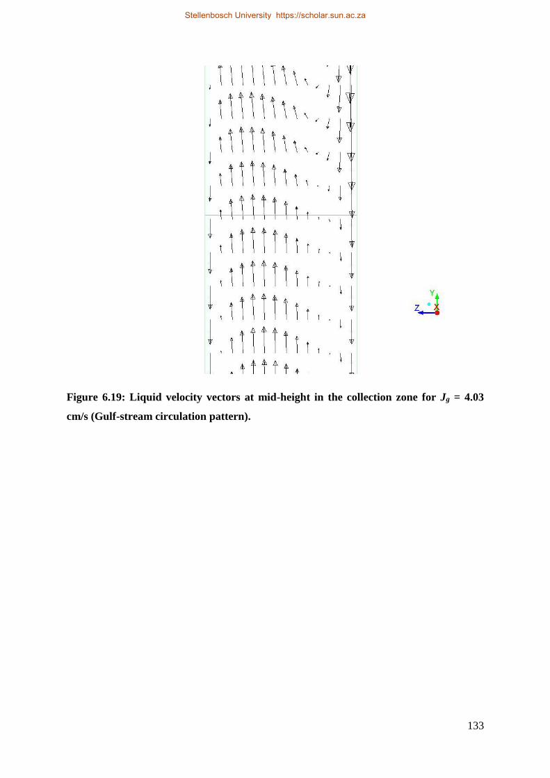
133
Figure 6.19: Liquid velocity vectors at mid-height in the collection zone for Jg = 4.03
cm/s (Gulf-stream circulation pattern).
Stellenbosch University https://scholar.sun.ac.za

134
Figure 6.20: Liquid velocity vectors at mid-height in the collection zone for Jg = 1.54
cm/s (Inverse circulation pattern).
6.5.5 Effect of interphase turbulent dispersion on radial gas holdup profile
The CFD results discussed in this work so far did not consider the interphase turbulent
dispersion forces in the simulations. However, turbulent dispersion, if taken into account,
might have an influence on the shape of the simulated radial gas holdup profiles. This is
because when turbulent dispersion forces are included in the simulations, turbulent
fluctuations will cause additional dispersion of phases from regions of high volume fraction
to regions of low volume fraction. In other words, the dispersed phase particles (or bubbles)
will be moving from areas of high concentration to low concentration areas. Turbulent
dispersion is therefore expected to have an effect on radial gas holdup profiles in the column.
The above concerns were addressed in this work by running some simulations in which the
model of Lopez de Bertodano [127] was used to determine the effect of turbulent dispersion
on the predicted radial gas holdup profile. The results are presented in Figure 6.21. Apart
from a small reduction of the peak gas holdup values near the column wall, it can be seen that
the turbulent dispersion did not have a significant influence on the shape of the gas holdup
Stellenbosch University https://scholar.sun.ac.za
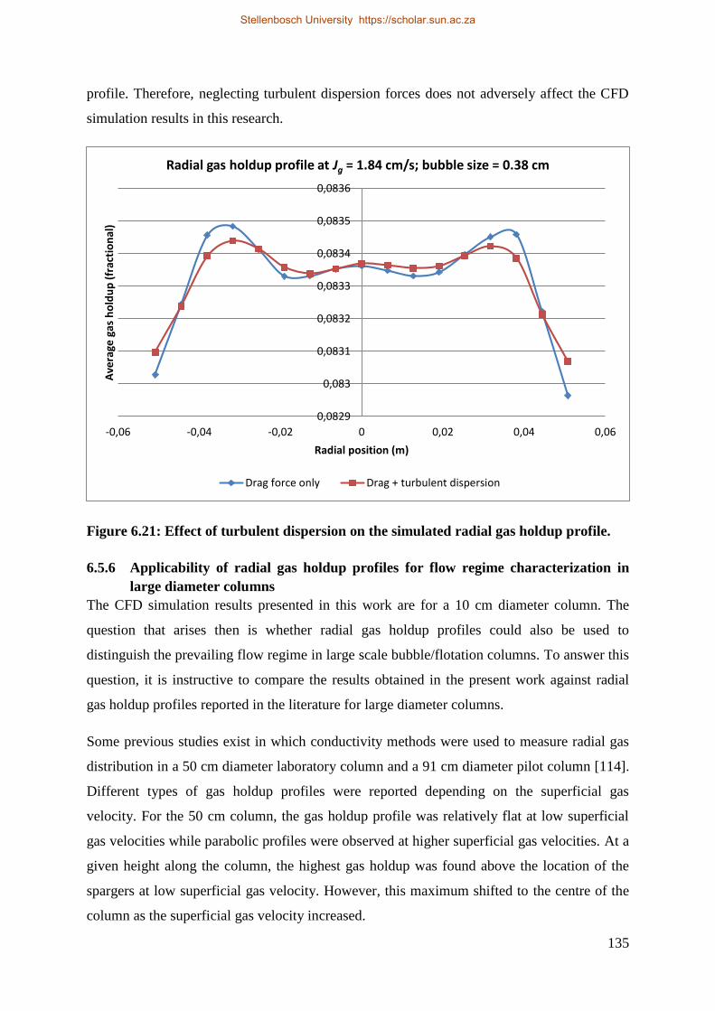
135
profile. Therefore, neglecting turbulent dispersion forces does not adversely affect the CFD
simulation results in this research.
Figure 6.21: Effect of turbulent dispersion on the simulated radial gas holdup profile.
6.5.6 Applicability of radial gas holdup profiles for flow regime characterization in
large diameter columns
The CFD simulation results presented in this work are for a 10 cm diameter column. The
question that arises then is whether radial gas holdup profiles could also be used to
distinguish the prevailing flow regime in large scale bubble/flotation columns. To answer this
question, it is instructive to compare the results obtained in the present work against radial
gas holdup profiles reported in the literature for large diameter columns.
Some previous studies exist in which conductivity methods were used to measure radial gas
distribution in a 50 cm diameter laboratory column and a 91 cm diameter pilot column [114].
Different types of gas holdup profiles were reported depending on the superficial gas
velocity. For the 50 cm column, the gas holdup profile was relatively flat at low superficial
gas velocities while parabolic profiles were observed at higher superficial gas velocities. At a
given height along the column, the highest gas holdup was found above the location of the
spargers at low superficial gas velocity. However, this maximum shifted to the centre of the
column as the superficial gas velocity increased.
0,0829
0,083
0,0831
0,0832
0,0833
0,0834
0,0835
0,0836
-0,06 -0,04 -0,02 0 0,02 0,04 0,06
Ave
rage
gas
ho
ldu
p (
frac
tio
nal
)
Radial position (m)
Radial gas holdup profile at Jg = 1.84 cm/s; bubble size = 0.38 cm
Drag force only Drag + turbulent dispersion
Stellenbosch University https://scholar.sun.ac.za
136
For the pilot column (91 cm diameter), radial gas holdup profiles were studied for Jg 0.60,
0.90, and 2.15 cm/s. The gas holdup profiles at low superficial gas velocities (Jg 0.60 and
0.90 cm/s) had a‘W’ shape with highest values observed near the column wall. The gas
holdup profiles then became saddle shaped as the superficial gas velocity increased to Jg =
2.15 cm/s.
From the above discussion, it is clear that there is a relationship between superficial gas
velocity and the shape of the radial gas holdup profile in the column. This relationship can be
employed to determine the prevailing flow regime in the column as has been demonstrated in
the present research.
6.6 Conclusions
In this study, the evolution of the shape of the radial gas holdup profile in a pilot scale
flotation column was studied using CFD to delineate the maximum gas velocity for loss of
bubbly flow. With increasing superficial gas velocity, the gas holdup profile undergoes
different stages which can be used to define the prevailing flow regime in the column. The
different flow regimes were also verified by the intensity of the local variations of the gas
holdup.
In the bubbly flow regime, saddle shaped and flat radial gas holdup profiles were obtained.
These profiles were accompanied by little to moderate gas holdup variations in the column.
The transition regime was gradual and characterised by flat to parabolic gas holdup profiles.
The parabolic profiles progressively became steeper as the superficial gas velocity increased.
The corresponding Gas holdup versus Time graphs in the transition regime showed moderate
to wide variations in gas holdup.
On the other hand, the churn-turbulent flow regime was distinguished by steep parabolic gas
holdup profiles with very wide variations in Gas holdup versus Time.
For conditions relevant to column flotation, the maximum superficial gas velocity was
determined for a column operating with an average bubble size of 1.5 mm and superficial
liquid velocity equal to 0.38 cm/s. The maximum superficial gas velocity was found to be
equal to 3.12 cm/s. The corresponding maximum gas holdup value was 20.1%.
Stellenbosch University https://scholar.sun.ac.za
137
Two possible flow patterns were revealed in the simulated column in this study, the gulf-
stream circulation pattern and an inverse circulation pattern. The latter was observed only in
the presence of fully developed saddle shaped radial gas holdup profiles.
Stellenbosch University https://scholar.sun.ac.za
138
Chapter 7 Conclusions and Recommendations
7.1 Research summary
The purpose of this research was to apply Computational Fluid Dynamics (CFD) to study gas
dispersion and mixing in industrial and pilot scale flotation columns. These two themes had
not been adequately addressed by previous CFD literature pertaining to column flotation. The
term gas dispersion combines three variables in minerals flotation: superficial gas velocity,
bubble size, and gas holdup. In addition, the bubble surface area flux, a fourth parameter
derived from the three, is used to characterize the flotation process. On the other hand, the
mixing processes in the column also affect its performance in terms of grade and recovery.
The CFD simulations in this research were performed using the Eulerian-Eulerian multiphase
model in which the different phases are considered separately as interpenetrating continua.
The Eulerian-Eulerian approach was selected among other models considering its lower
computational cost compared with other models such as the Eulerian-Lagrangian. These other
models are limited to simulating systems in which the dispersed phase volume fractions are
considerably low (less than 10% for Eulerian-Lagrangian model). The interaction between
the phases in the Eulerian-Eulerian model was accounted for by means of the drag force only
while other forces such as virtual mass and lift force were assumed to be negligible based on
literature evidence.
In the CFD simulations, the flow variables are calculated by solving the Reynolds averaged
momentum and continuity equations. In addition, the turbulence model is solved in order to
account for the effects of turbulence fluctuations on the mean flow. The turbulence in the
continuous liquid phase in the columns was modelled using the Realizable k-ϵ turbulence
model. On the other hand, previous CFD models of column flotation in the literature have
used the Standard k-ϵ model while others have assumed laminar flow conditions. It would
therefore be necessary to investigate the effect of using different turbulence models on the
simulated flow variables. However, this aspect was not studied in the present research in the
context of column flotation due to lack of experimental data against which to compare the
models.
An important aspect of the research involves the definition of a suitable computational
domain for the flotation column CFD model. Due to the differences in flow patterns and
turbulence characteristics between the collection zone and the froth zone, it still remains a
Stellenbosch University https://scholar.sun.ac.za
139
challenge to formulate CFD simulations that combine the two zones. The focus of this
research was therefore the collection zone of the column while the froth phase was not
included in the model.
Further simplifications were achieved in this research by excluding the spargers from the
model geometry. Instead, the air bubbles were introduced into the column over the entire
column cross section at the bottom of the vessel. Considering the uniform gas holdup
distributions that are achievable with flotation column spargers, introducing air bubbles over
the entire column section is a reasonable albeit simplified representation of the actual
sparging mechanism.
The formulated CFD methodology was subsequently used to study the following three
aspects of column flotation:
Gas holdup and its axial variation along the column
Mixing characteristics of the collection zone, and
Flow regime transition in the column
The main conclusions of the research are summarized in the next section within the context
of these three issues. The axial gas holdup variation in the column was achieved by imposing
compressibility effects on the bubbles using the Ideal Gas law. The actual hydrostatic
expansion of the bubbles was not modelled. The CFD model therefore accounts for changes
in bubble density in response to the local hydrostatic pressure value while the bubble size
remains constant throughout the column. However, the results obtained compared favourably
with experimental data.
The mixing characteristics of the liquid phase (water) in industrial flotation columns were
simulated using the Species model available in the Ansys Fluent CFD solver. On the other
hand, the particle (solids) mean residence time was determined scalar transport equation that
computes the age of particles to give their spatial age distribution in the column. The mean
residence time is then obtained as the area weighted average age of the particles at the outlet.
This method has been used to predict mean residence time in the chemical engineering
literature. However, this research is the first to apply the method for column flotation studies.
An advantage of using this particle age equation is that it has less computational cost
compared to other methods such as Lagrangian particle tracking. In addition, this method
Stellenbosch University https://scholar.sun.ac.za

140
provides further insights into the effects of liquid recirculation on particle residence time in
the column.
The final part of this research investigated flow regime transition in a pilot scale column cell.
The well-known method in which the superficial gas velocity is plotted against gas holdup
was used to predict flow regime transition for a system with water and air only (without
frother). However, the method could not be applied to model a system with frother due to the
unavailability of methods to calculate the mean bubble sizes that could be used in the
simulations for the column in the churn-turbulent regime. The effect of superficial gas
velocity on radial gas holdup profiles was therefore studied in order to distinguish the flow
regime on the basis of the gas holdup profiles under conditions relevant to column flotation.
A CFD model coupled with a Bubble Population Balance model might be more suitable for
simulating columns in the churn-turbulent regime because bubble size distributions can then
be incorporated in the model.
7.2 Conclusions
7.2.1 Gas holdup and its distribution in the column
Gas holdup was observed to increase with height along the column as reported in the
literature. The gas holdup increased by more than 100% from the bottom to the top part of the
column over a height of 13.5 m. An axial profile of bubble velocity was observed in which
bubble velocity increased rapidly to a maximum value and then began to decrease with height
to a terminal velocity. This study attributes the axial decrease in bubble velocity to a possible
increase in drag force resulting from increasing gas holdup along the column height. It is also
argued that the decrease in bubble velocity will further increase the gas holdup profile due to
increased bubble residence time. This study therefore proposes that the axial increase in gas
holdup maybe inter-related with the axial bubble velocity reduction observed along the
column axis.
7.2.2 Mixing characteristics of the collection zone in column flotation
In terms of mixing in the column, the formulated CFD model was used to simulate the liquid
RTDs in order to determine the mixing parameters (the vessel dispersion number and the
mean residence time) for the column. The model was capable of predicting mixing
parameters comparable with experimental data for both square and cylindrical industrial
columns. This research further investigated the effect of liquid circulation on the particle
residence time. It was found that the spatial age distribution of the particles in the column is
Stellenbosch University https://scholar.sun.ac.za

141
related to the prevailing liquid circulation flow pattern. The effects of solids particle size and
bubble size on the liquid dispersion in the column were also studied. The CFD simulation
results showed that the liquid dispersion is affected by particle size and bubble size.
Increasing the particle size of the solids resulted in a decrease in the liquid vessel dispersion
number. On the other hand, a decrease in bubble size resulted in an increase in the liquid
vessel dispersion number.
7.2.3 Flow regime identification using CFD
Flow regime transition was identified for a water and air system (without frother) using gas
holdup versus superficial gas velocity graphs derived from CFD simulations. Radial gas
holdup profiles were then studied for the delineated flow regimes in order to determine
whether gas holdup profiles could be used to indicate the prevailing flow pattern in the
column. In this regard, the bubbly flow regime can be characterized by three distinct radial
gas holdup profiles as follows:
saddle shaped profiles with three peaks at lower superficial gas velocities
Saddle shaped profiles with two near wall peaks and a central minimum as the
superficial gas velocity increases
Flat gas holdup profiles just before transition towards churn turbulent flow. In some
cases the profiles appear to have intermediate features between saddle and parabolic
gas holdup profiles
The transition regime was characterized by flat profiles that evolved into parabolic profiles as
the superficial gas velocity increased. The transition regime was therefore seen to be gradual
which would make it difficult to use radial gas holdup profiles to determine the maximum gas
velocity in column flotation. However, parabolic radial gas holdup profiles would certainly
indicate that the column is operating under churn turbulent flow conditions.
The prevailing flow patterns in the column were further confirmed using gas holdup versus
time graphs. The two extreme conditions of bubbly flow and churn turbulent flow were easier
to distinguish. In this case, the gas holdup remained constant in the bubbly flow regime while
churn turbulent flow was characterized by wide variations in the gas holdup. The transition
regime was again gradual in which the gas holdup versus time graphs show moderate to wide
fluctuations as the superficial gas velocity increases.
Stellenbosch University https://scholar.sun.ac.za

142
Another important observation emerging from this research was that different radial gas
holdup profiles could result in opposite liquid flow patterns. For example, a liquid circulation
pattern with upward flow in the centre and downward flow near the column walls was always
present when the gas holdup profile is parabolic. On the other hand, an inverse flow pattern
was observed in which the liquid rises near the column wall but descends in the centre and
adjacent to the wall. This profile was accompanied by corresponding saddle shaped gas
holdup profiles.
7.3 Recommendations
The following recommendations can be considered for future research:
For the work on gas holdup and its distribution in the column, it is recommended for
future research to incorporate the actual bubble expansion as a function of height or
hydrostatic pressure inside the column. This aspect was neglected in the present
research in order to achieve a simplified CFD model and also to reduce the
computational effort required to perform the simulations.
The present research has investigated the relationship between radial gas holdup
profiles and the prevailing flow pattern in a 0.1 m diameter column. It would be
important in future studies to find out whether radial gas holdup profiles can be used
to distinguish flow regimes in industrial flotation columns. Radial gas holdup profiles
should therefore be studied in larger columns in the context of flow regime
characterization.
The CFD simulations in the present study assumed a constant average bubble size for
all the columns. However, for the churn turbulent regime, a bubble size distribution
exists which could have an effect on the hydrodynamics of the column. On the other
hand, a bubble population balance model can be used to predict bubble size
distributions in the column. It is therefore recommended for future research to apply
CFD models coupled with bubble population balance models when simulating
different flow regimes in the column.
Some of the CFD models in the literature have used the standard k-ϵ model to account
for turbulence while others have assumed laminar conditions. It would be helpful to
compare the different turbulence models in terms of their prediction of flow variables
in future studies.
Stellenbosch University https://scholar.sun.ac.za
143
References
References
1. Wheeler D. In: Column flotation-the original column. Proceedings of 2nd latin american
congress in froth flotation (SH castro, J. alvarez eds.); ; 1985. p. 19-23.
2. Finch JA, Dobby GS. Column flotation. Oxford, England: Pergamon Press; 1990.
3. Finch J, Hardie C. An example of innovation from the waste management industry:
Deinking flotation cells. Minerals Eng. 1999;12(5):467-75.
4. Hernandez H, Gomez C, Finch J. Gas dispersion and de-inking in a flotation column.
Minerals Eng. 2003;16(8):739-44.
5. Finch J, Xiao J, Hardie C, Gomez C. Gas dispersion properties: Bubble surface area flux
and gas holdup. Minerals Eng. 2000;13(4):365-72.
6. Matiolo E, Testa F, Yianatos J, Rubio J. On the gas dispersion measurements in the
collection zone of flotation columns. Int J Miner Process. 2011;99(1):78-83.
7. Ityokumbul M. A new modelling approach to flotation column desing. Minerals Eng.
1992;5(6):685-93.
8. Yianatos J, Finch J. Gas holdup versus gas rate in the bubbly regime. Int J Miner Process.
1990;29(1):141-6.
9. Mavros P. Mixing in flotation columns. part I: Axial dispersion modelling. Minerals Eng.
1993;6(5):465-78.
Stellenbosch University https://scholar.sun.ac.za
144
10. Mavros P, Daniilidou A. Mixing in flotation columns. part II. liquid-phase residence time
distributions studies. Minerals Eng. 1993;6(7):707-19.
11. Deng H, Mehta R, Warren G. Numerical modeling of flows in flotation columns. Int J
Miner Process. 1996;48(1):61-72.
12. Koh P, Schwarz M, Zhu Y, Bourke P, Peaker R, Franzidis J. In: Development of CFD
models of mineral flotation cells. Third international conference on computational fluid
dynamics in the minerals and process industries, melbourne, australia; ; 2003. p. 171-5.
13. Koh P, Schwarz M. In: CFD models of microcel and jameson flotation cells. Seventh
international conference on CFD in the minerals and process industries, CSIRO, melbourne,
australia; ; 2009.
14. Chakraborty D, Guha M, Banerjee P. CFD simulation on influence of superficial gas
velocity, column size, sparger arrangement, and taper angle on hydrodynamics of the column
flotation cell. Chem Eng Commun. 2009;196(9):1102-16.
15. Xia Y, Peng F, Wolfe E. CFD simulation of alleviation of fluid back mixing by baffles in
bubble column. Minerals Eng. 2006;19(9):925-37.
16. Nadeem M, Ahmed J, Chughtai IR, Ullah A. CFD-based estimation of collision
probabilities between fine particles and bubbles having intermediate reynolds number.
Nucleus. 2009;46(3):153-9.
17. Rehman A, Nadeem M, Zaman M, Nadeem B. Effect of various baffle designs on air
holdup and mixing in a flotation column using CFD. . 2011.
Stellenbosch University https://scholar.sun.ac.za

145
18. Gomez C, Uribe-Salas A, Finch J, Huls B. Gas holdup measurement in flotation columns
using electrical conductivity. Can Metall Q. 1991;30(4):201-5.
19. Xu M, Uribe-Salas A, Finch J, Gomez C. In: Gas rate limitation in column flotation.
Processing of complex ores: Proceedings of the international symposium on processing of
complex ores, halifax, august 20-24, 1989; Elsevier; 1989. p. 397.
20. Xu M, Finch J, Uribe-Salas A. Maximum gas and bubble surface rates in flotation
columns. Int J Miner Process. 1991;32(3):233-50.
21. Langberg D, Jameson G. The coexistence of the froth and liquid phases in a flotation
column. Chemical engineering science. 1992;47(17):4345-55.
22. Schallenberg J, Enß JH, Hempel DC. The important role of local dispersed phase hold-
ups for the calculation of three-phase bubble columns. Chemical engineering science.
2005;60(22):6027-33.
23. Cilliers J. In: Understanding froth behaviour with CFD. 5th international conference on
CFD in the process industries CSIRO, melbourne; ; 2006.
24. Dobby GS. A fundamental flotation model and flotation column scale-up [dissertation].
Montreal, Canada: McGill University; 1985.
25. Dobby G, Finch J. Column flotation: A selected review, part II. Minerals Eng.
1991;4(7):911-23.
26. Harach PL, Redfearn MA, Waites DB, inventors; Cominco Ltd. V, Canada, assignee.
United States patent 4,911,826. 1990 .
Stellenbosch University https://scholar.sun.ac.za
146
27. Xu M, Finch J, Huls B. Measurement of radial gas holdup profiles in a flotation column.
Int J Miner Process. 1992;36(3):229-44.
28. Paleari F, Xu M, Finch J. Radial gas holdup profiles: The influence of sparger systems.
Minerals and Metallurgical Processing. 1994;11(2):111-7.
29. Yianatos J, Bergh L, Sepulveda C, Núñez R. Measurement of axial pressure profiles in
large-size industrial flotation columns. Minerals Eng. 1995;8(1):101-9.
30. Zhou Z, Egiebor N. Prediction of axial gas holdup profiles in flotation columns. Minerals
Eng. 1993;6(3):307-12.
31. Sam A, Gomez C, Finch J. Axial velocity profiles of single bubbles in water/frother
solutions. Int J Miner Process. 1996;47(3):177-96.
32. Michele V, Hempel DC. Liquid flow and phase holdup—measurement and CFD
modeling for two-and three-phase bubble columns. Chemical engineering science.
2002;57(11):1899-908.
33. Baléo J, Le Cloirec P. Validating a prediction method of mean residence time spatial
distributions. AIChE J. 2000;46(4):675-83.
34. Baléo J, Humeau P, Le Cloirec P. Numerical and experimental hydrodynamic studies of a
lagoon pilot. Water Res. 2001;35(9):2268-76.
35. Ghirelli F, Leckner B. Transport equation for the local residence time of a fluid. Chemical
engineering science. 2004;59(3):513-23.
36. Liu M, Tilton J. Spatial distributions of mean age and higher moments in steady
continuous flows. AIChE J. 2010;56(10):2561-72.
Stellenbosch University https://scholar.sun.ac.za
147
37. Simcik M, Ruzicka M, Mota A, Teixeira J. Smart RTD for multiphase flow systems.
Chem Eng Res Design. 2012;90(11):1739-49.
38. Ityokumbul M. Maximum gas velocity in column flotation. Minerals Eng.
1993;6(12):1279-86.
39. Dobby G, Finch J. Particle collection in columns—gas rate and bubble size effects. Can
Metall Q. 1986;25(1):9-13.
40. Finch JA, Dobby GS. Column flotation: A selected review. part I. Int J Miner Process.
1991;33(1):343-54.
41. Leichtle GF. Analysis of bubble generating devices in a deinking column [dissertation].
McGill University; 1998.
42. López-Saucedo F, Uribe-Salas A, Pérez-Garibay R, Magallanes-Hernández L. Gas
dispersion in column flotation and its effect on recovery and grade. Can Metall Q.
2012;51(2):111-7.
43. Massinaei M, Kolahdoozan M, Noaparast M, Oliazadeh M, Yianatos J, Shamsadini R, et
al. Hydrodynamic and kinetic characterization of industrial columns in rougher circuit.
Minerals Eng. 2009;22(4):357-65.
44. Dobby G, Amelunxen R, Finch J. In: Column flotation: Some plant experience and model
development. Symposium on automation for mineral development; ; 1985. p. 9-11.
45. Gomez C, Uribe-Salas A, Finch J, Huls B. Axial gas holdup profiles in the collection
zones of flotation columns. Minerals and Metallurgical Processing. 1995;12(1):16-23.
Stellenbosch University https://scholar.sun.ac.za

148
46. Serizawa A, Kataoka I, Michiyoshi I. Turbulence structure of air-water bubbly flow—II.
local properties. Int J Multiphase Flow. 1975;2(3):235-46.
47. Bennett M, Luke S, Jia X, West R, Williams R. In: Analysis and flow regime
identification of bubble column dynamics. 1st world congress on industrial process
tomography, buxton, greater manchester; ; 1999. p. 14-7.
48. Hills J. Radial non-uniformity of velocity and voidage in a bubble column.
Trans.Inst.Chem.Eng. 1974;52(1):1-9.
49. Freedman W, Davidson J. Hold-up and liquid circulation in bubble columns. Transactions
of the Institution of Chemical Engineers and the Chemical Engineer. 1969;47(8):T251.
50. Devanathan N, Moslemian D, Dudukovic M. Flow mapping in bubble columns using
CARPT. Chemical Engineering Science. 1990;45(8):2285-91.
51. Clark N, Atkinson C, Flemmer R. Turbulent circulation in bubble columns. AIChE J.
1987;33(3):515-8.
52. Dobby G, Yianatos J, Finch J. Estimation of bubble diameter in flotation columns from
drift flux analysis. Can Metall Q. 1988;27(2):85-90.
53. Yianatos J, Finch J, Dobby G, Xu M. Bubble size estimation in a bubble swarm. J Colloid
Interface Sci. 1988;126(1):37-44.
54. Banisi S, Finch JA. Technical note reconciliation of bubble size estimation methods using
drift flux analysis. Minerals Eng. 1994 12;7(12):1555-9.
Stellenbosch University https://scholar.sun.ac.za

149
55. López-Saucedo F, Uribe-Salas A, Pérez-Garibay R, Magallanes-Hernández L, Lara-
Valenzuela C. Modelling of bubble size in industrial flotation columns. Can Metall Q.
2011;50(2):95-101.
56. Luttrell G, Mankosa M, Yoon R. In: Design and scale-up criteria for column flotation.
XVIII international mineral processing congress; ; 1993. p. 785-91.
57. Rice R, Oliver A, Newman J, Wiles R. Reduced dispersion using baffles in column
flotation. Powder Technol. 1974;10(4):201-10.
58. Dobby G, Finch J. Mixing characteristics of industrial flotation columns. Chemical
Engineering Science. 1985;40(7):1061-8.
59. Laplante A, Yianatos J, Finch J. On the mixing characteristics of the collection zone in
flotation columns. Column flotation. 1988;88:69-80.
60. Mavros P, Lazaridis N, Matis K. A study and modelling of liquid-phase mixing in a
flotation column. Int J Miner Process. 1989;26(1):1-16.
61. Goodall C, O'Connor C. Residence time distribution studies in a flotation column. part 1:
The modelling of residence time distributions in a laboratory column flotation cell. Int J
Miner Process. 1991;31(1):97-113.
62. Goodall C, O'Connor C. Residence time distribution studies in a flotation column. part 2:
The relationship between solids residence time distribution and metallurgical performance.
Int J Miner Process. 1992;36(3):219-28.
63. Mankosa M, Luttrell G, Adel G, Yoon R. A study of axial mixing in column flotation. Int
J Miner Process. 1992;35(1):51-64.
Stellenbosch University https://scholar.sun.ac.za

150
64. Xu M, Finch J. Solids mixing in the collection zone of flotation columns. Minerals Eng.
1992;5(9):1029-39.
65. Yianatos JB, Bergh LG. RTD studies in an industrial flotation column: Use of the
radioactive tracer technique. Int J Miner Process. 1992;36(1):81-91.
66. Yianatos JB, Bergh LG, Díaz F, Rodríguez J. Mixing characteristics of industrial flotation
equipment. Chemical Engineering Science. 2005;60(8):2273-82.
67. Massinaei M, Kolahdoozan M, Noaparast M, Oliazadeh M, Sahafipour M, Finch J.
Mixing characteristics of industrial columns in rougher circuit. Minerals Eng.
2007;20(15):1360-7.
68. Schwarz M. Flow simulation in minerals engineering. Minerals Eng. 1991;4(7):717-32.
69. Napier-Munn TJ, Lynch A. The modelling and computer simulation of mineral treatment
processes—current status and future trends. Minerals Eng. 1992;5(2):143-67.
70. Anderson JD. Computational fluid dynamics. McGraw-Hill; 1995.
71. Versteeg HK, Malalasekera W. An introduction to computational fluid dynamics: The
finite volume method. Prentice Hall; 2007.
72. Andersson B, Andersson R, Håkansson L, Mortensen M, Sudiyo R. Computational fluid
dynamics for engineers. Cambridge University Press; 2011.
73. Yianatos J, Bergh L, Sepulveda C, Núñez R. Measurement of axial pressure profiles in
large-size industrial flotation columns. Minerals Eng. 1995;8(1):101-9.
Stellenbosch University https://scholar.sun.ac.za
151
74. Sato Y, Sekoguchi K. Liquid velocity distribution in two-phase bubble flow. Int J
Multiphase Flow. 1975;2(1):79-95.
75. Sarhan A, Naser J, Brooks G. CFD simulation on influence of suspended solid particles
on bubbles' coalescence rate in flotation cell. Int J Miner Process. 2016;146:54-64.
76. Brito-Parada P, Neethling S, Cilliers J. The advantages of using mesh adaptivity when
modelling the drainage of liquid in froths. Minerals Eng. 2012;33:80-6.
77. Sasic S, Sibaki EK, Ström H. Direct numerical simulation of a hydrodynamic interaction
between settling particles and rising microbubbles. European Journal of Mechanics-B/Fluids.
2014;43:65-75.
78. Andersson B, Andersson R, Håkansson L, Mortensen M, Sudiyo R, van Wachem B.
Computational fluid dynamics for engineers. Cambridge University Press; 2011.
79. Ranade VV. Computational flow modeling for chemical reactor engineering. Academic
press; 2001.
80. Delnoij E, Kuipers JAM, van Swaaij WPM. Computational fluid dynamics applied to
gas-liquid contactors. Chemical Engineering Science. 1997 11;52(21–22):3623-38.
81. Zhang D. Eulerian modeling of reactive gas-liquid flow in a bubble column. University of
Twente; 2007.
82. Akhtar A. Two-fluid eulerian simulation of bubble column reactors with distributors. J
Chem Eng Japan. 2006;39(8):831-41.
83. Chen P, Sanyal J, Dudukovic M. CFD modeling of bubble columns flows:
Implementation of population balance. Chemical Engineering Science. 2004;59(22):5201-7.
Stellenbosch University https://scholar.sun.ac.za

152
84. Chen P, Duduković M, Sanyal J. Three‐dimensional simulation of bubble column flows
with bubble coalescence and breakup. AIChE J. 2005;51(3):696-712.
85. Chen J, Yang N, Ge W, Li J. Computational fluid dynamics simulation of regime
transition in bubble columns incorporating the dual-bubble-size model. Ind Eng Chem Res.
2009;48(17):8172-9.
86. Sahbaz O, Ercetin U, Oteyaka B. Determination of turbulence and upper size limit in
jameson flotation cell by the use of computational fluid dynamic modelling. Physicochemical
Problems of Mineral Processing. 2012;49(2):535-46.
87. Yan X, Liu J, Cao Y, Wang L. A single-phase turbulent flow numerical simulation of a
cyclonic-static micro bubble flotation column. International Journal of Mining Science and
Technology. 2012;22(1):95-100.
88. Mavros P, Daniilidou A, Papatsiotsou F. Internal recirculation and mixing in flotation
columns. Trans IChemE. 1995;73(Part A).
89. Karthik T, Durst F. Turbulence models and their applications. Department of Mechanical
Engineering, Indian Institute of Technology, Madras, India. 2011.
90. Launder BE, Spalding D. The numerical computation of turbulent flows. Comput
Methods Appl Mech Eng. 1974;3(2):269-89.
91. Laborde-Boutet C, Larachi F, Dromard N, Delsart O, Schweich D. CFD simulation of
bubble column flows: Investigations on turbulence models in RANS approach. Chemical
Engineering Science. 2009;64(21):4399-413.
Stellenbosch University https://scholar.sun.ac.za
153
92. Pfleger D, Gomes S, Gilbert N, Wagner H. Hydrodynamic simulations of laboratory scale
bubble columns fundamental studies of the Eulerian–Eulerian modelling approach. Chemical
Engineering Science. 1999;54(21):5091-9.
93. Pfleger D, Becker S. Modelling and simulation of the dynamic flow behaviour in a bubble
column. Chemical Engineering Science. 2001 2;56(4):1737-47.
94. NI K. Multiphase flow dynamics, vol. 2 thermal and mechanical interactions. 2nd ed.
Berlin, Germany: Springer; 2005.
95. Schiller L, Naumann A. A drag coefficient correlation. Vdi Zeitung. 1935;77:318-20.
96. Morsi S, Alexander A. An investigation of particle trajectories in two-phase flow
systems. J Fluid Mech. 1972;55(2):193-208.
97. Zhou Z, Egiebor N. Technical note a gas-liquid drift-flux model for flotation columns.
Minerals Eng. 1993;6(2):199-205.
98. Yianatos J, Bergh L, Durán O, Diaz F, Heresi N. Measurement of residence time
distribution of the gas phase in flotation columns. Minerals Eng. 1994;7(2):333-44.
99. Prince MJ, Blanch HW. Bubble coalescence and break‐up in air‐sparged bubble columns.
AIChE J. 1990;36(10):1485-99.
100. López-Saucedo F, Uribe-Salas A, Pérez-Garibay R, Magallanes-Hernández L, Lara-
Valenzuela C. Modelling of bubble size in industrial flotation columns. Can Metall Q.
2011;50(2):95-101.
101. Nicklin D. Two-phase bubble flow. Chemical engineering science. 1962;17(9):693-702.
Stellenbosch University https://scholar.sun.ac.za

154
102. Zhou Z, Egiebor N, Plitt L. Frother effects on bubble motion in a swarm. Can Metall Q.
1993;32(2):89-96.
103. Mills P, Yianatos J, O'Connor C. The mixing characteristics of solid and liquid phases in
a flotation column. Minerals Eng. 1992;5(10):1195-205.
104. Yianatos JB, Bergh LG, Díaz F, Rodríguez J. Mixing characteristics of industrial
flotation equipment. Chemical Engineering Science. 2005;60(8):2273-82.
105. Ityokumbul M. A new modelling approach to flotation column desing. Minerals Eng.
1992;5(6):685-93.
106. Mills P, O'Connor C. The modelling of liquid and solids mixing in a flotation column.
Minerals Eng. 1990;3(6):567-76.
107. Levenspiel O. Chemical reaction engineering. Wiley Eastern Limited; 1972.
108. Chen J, Gupta P, Degaleesan S, Al-Dahhan MH, Duduković MP, Toseland BA. Gas
holdup distributions in large-diameter bubble columns measured by computed tomography.
Flow Meas Instrum. 1998;9(2):91-101.
109. Delnoij E. Fluid dynamics of gas-liquid bubble columns [dissertation]. Universiteit
Twente; 1999.
110. Wen C, Yu Y. In: Mechanics of fluidization. Chem. eng. prog. symp. ser. ; 1966. p. 100-
11.
111. Ring T, Wang B, Sang-Choi B, Dhanasekharan K. Predicting residence time distribution
with FLUENT. Fluent News. 2004;31.
Stellenbosch University https://scholar.sun.ac.za
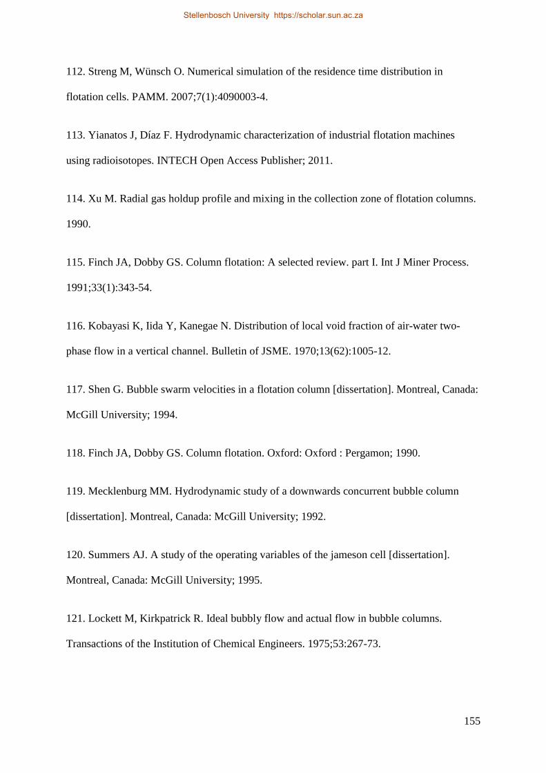
155
112. Streng M, Wünsch O. Numerical simulation of the residence time distribution in
flotation cells. PAMM. 2007;7(1):4090003-4.
113. Yianatos J, Díaz F. Hydrodynamic characterization of industrial flotation machines
using radioisotopes. INTECH Open Access Publisher; 2011.
114. Xu M. Radial gas holdup profile and mixing in the collection zone of flotation columns.
1990.
115. Finch JA, Dobby GS. Column flotation: A selected review. part I. Int J Miner Process.
1991;33(1):343-54.
116. Kobayasi K, Iida Y, Kanegae N. Distribution of local void fraction of air-water two-
phase flow in a vertical channel. Bulletin of JSME. 1970;13(62):1005-12.
117. Shen G. Bubble swarm velocities in a flotation column [dissertation]. Montreal, Canada:
McGill University; 1994.
118. Finch JA, Dobby GS. Column flotation. Oxford: Oxford : Pergamon; 1990.
119. Mecklenburg MM. Hydrodynamic study of a downwards concurrent bubble column
[dissertation]. Montreal, Canada: McGill University; 1992.
120. Summers AJ. A study of the operating variables of the jameson cell [dissertation].
Montreal, Canada: McGill University; 1995.
121. Lockett M, Kirkpatrick R. Ideal bubbly flow and actual flow in bubble columns.
Transactions of the Institution of Chemical Engineers. 1975;53:267-73.
Stellenbosch University https://scholar.sun.ac.za

156
122. Ruzicka M, Zahradnık J, Drahoš J, Thomas N. Homogeneous–heterogeneous regime
transition in bubble columns. Chemical Engineering Science. 2001;56(15):4609-26.
123. Vial C, Poncin S, Wild G, Midoux N. A simple method for regime identification and
flow characterisation in bubble columns and airlift reactors. Chemical Engineering and
Processing: Process Intensification. 2001;40(2):135-51.
124. Shaikh A, Al-Dahhan MH. A review on flow regime transition in bubble columns.
International Journal of Chemical Reactor Engineering. 2007;5(1).
125. Lin J, Chen M, Chao B. A novel radioactive particle tracking facility for measurement
of solids motion in gas fluidized beds. AIChE J. 1985;31(3):465-73.
126. Clark N, Van Egmond J, Nebiolo E. The drift-flux model applied to bubble columns and
low velocity flows. Int J Multiphase Flow. 1990;16(2):261-79.
127. de Bertodano, Martin Aurelio Lopez. Turbulent bubbly two-phase flow in a triangular
duct. 1992.
Stellenbosch University https://scholar.sun.ac.za

157
Appendix 1: Mass and momentum source terms for the simulations in
Chapter 4 .
This Appendix presents the mass and momentum source terms calculated from superficial gas
velocities using equations (3.1) and (3.2)as described in Chapter 3.
Superficial Gas
Velocity ( cm/s)
Superficial Gas
Velocity ( m/s)
Mass Source term (
kg/ m3 - s )
Momentum Source
term ( N/ m3 )
0.72 0.0072 8.82E-01 6.35E-03
0.93 0.0093 1.14E+00 1.06E-02
1.22 0.0122 1.49E+00 1.82E-02
1.51 0.0151 1.85E+00 2.79E-02
1.67 0.0167 2.05E+00 3.42E-02
Stellenbosch University https://scholar.sun.ac.za

158
Appendix 2: User defined function for the source term used in particle age
transport equation
This Appendix outlines the user defined function (UDF) that was used to calculate the source
term in the particle age user defined scalar (UDS) equation described in Chapter 5, equation
(5.18) ).
#include "udf.h"
DEFINE_SOURCE(my_scalar_source,c,t,ds,eqn)
{
real source;
real rho_p = C_R(c,t);
real vof_p = C_VOF(c,t);
source = rho_p*vof_p;
ds[eqn] = 0;
return source;
}
Stellenbosch University https://scholar.sun.ac.za
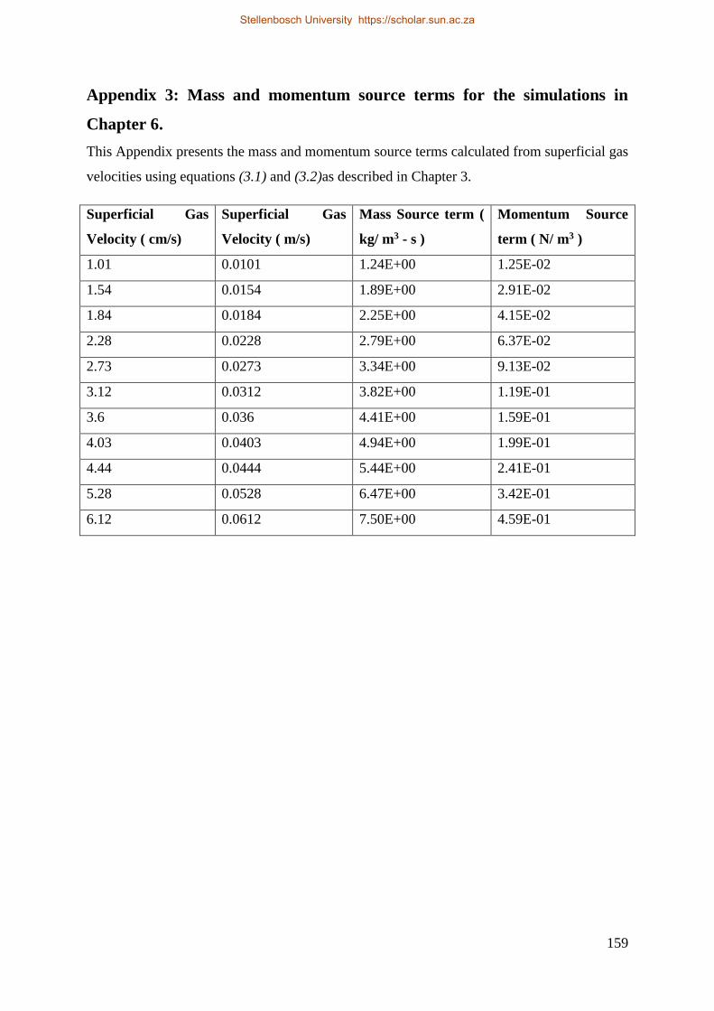
159
Appendix 3: Mass and momentum source terms for the simulations in
Chapter 6.
This Appendix presents the mass and momentum source terms calculated from superficial gas
velocities using equations (3.1) and (3.2)as described in Chapter 3.
Superficial Gas
Velocity ( cm/s)
Superficial Gas
Velocity ( m/s)
Mass Source term (
kg/ m3 - s )
Momentum Source
term ( N/ m3 )
1.01 0.0101 1.24E+00 1.25E-02
1.54 0.0154 1.89E+00 2.91E-02
1.84 0.0184 2.25E+00 4.15E-02
2.28 0.0228 2.79E+00 6.37E-02
2.73 0.0273 3.34E+00 9.13E-02
3.12 0.0312 3.82E+00 1.19E-01
3.6 0.036 4.41E+00 1.59E-01
4.03 0.0403 4.94E+00 1.99E-01
4.44 0.0444 5.44E+00 2.41E-01
5.28 0.0528 6.47E+00 3.42E-01
6.12 0.0612 7.50E+00 4.59E-01
Stellenbosch University https://scholar.sun.ac.za

160
Appendix 4: Drag coefficient calculations used for the CD versus Re graphs
in Figure 4.6.
A. Schiller Naumann
Re CD ;𝐶𝐷 =24
𝑅𝑒(1 + 0.15𝑅𝑒0.687)
50 1,538095554
100 1,091731091
150 0,910215334
200 0,805614687
250 0,735362673
300 0,68389794
350 0,64402356
400 0,611896606
450 0,585254147
500 0,562665302
550 0,543174879
600 0,526117392
650 0,511012886
700 0,497505194
750 0,485323596
800 0,474258079
850 0,46414283
900 0,454844909
950 0,446256291
1000 0,43828814
Stellenbosch University https://scholar.sun.ac.za
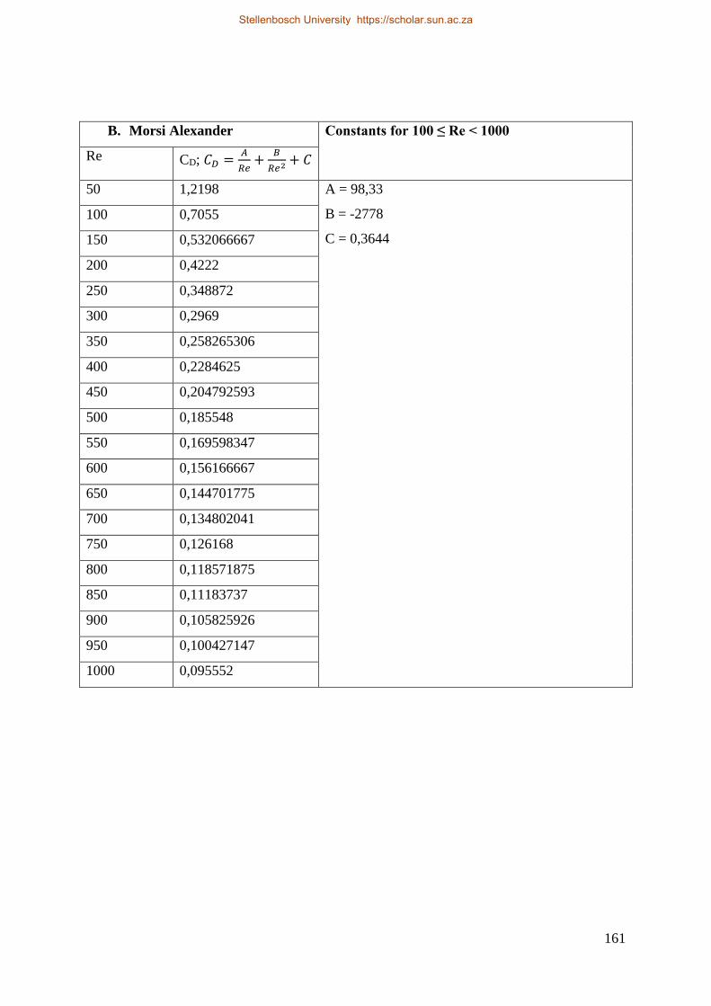
161
B. Morsi Alexander Constants for 100 ≤ Re < 1000
Re CD; 𝐶𝐷 =𝐴
𝑅𝑒+
𝐵
𝑅𝑒2 + 𝐶
50 1,2198 A = 98,33
B = -2778
C = 0,3644
100 0,7055
150 0,532066667
200 0,4222
250 0,348872
300 0,2969
350 0,258265306
400 0,2284625
450 0,204792593
500 0,185548
550 0,169598347
600 0,156166667
650 0,144701775
700 0,134802041
750 0,126168
800 0,118571875
850 0,11183737
900 0,105825926
950 0,100427147
1000 0,095552
Stellenbosch University https://scholar.sun.ac.za
162
C. Universal drag: Viscous region (0 ≤ Reb < 1000)
Re CD; 𝐶𝐷𝑉𝑖𝑠=
24
𝑅𝑒(1 + 0.1𝑅𝑒0.75)
50 1,382544742
100 0,998946638
150 0,845785703
200 0,758195508
250 0,699568046
300 0,656674739
350 0,623445244
400 0,596656315
450 0,574417783
500 0,555538206
550 0,539224121
600 0,524923721
650 0,51223959
700 0,500877116
750 0,49061254
800 0,481272371
850 0,472719681
900 0,464844713
950 0,457558285
1000 0,450787058
Stellenbosch University https://scholar.sun.ac.za

163
Appendix 5: Predicted turbulence quanties at mid-height position for the
column (0.91 m diameter) simulated in Chapter 4.
0
0,5
1
1,5
2
2,5
3
3,5
4
-0,6 -0,4 -0,2 0 0,2 0,4 0,6
Turb
ule
nt
Vis
cosi
ty (
kg/m
-s)
Radial position (m)
Turbulent Viscosity (water)
0
0,5
1
1,5
2
2,5
3
3,5
4
-0,6 -0,4 -0,2 0 0,2 0,4 0,6
Effe
ctiv
e V
isco
sity
(kg
/m-s
)
Radial position (m)
Effective Viscosity (water)
Stellenbosch University https://scholar.sun.ac.za

164
0
0,0005
0,001
0,0015
0,002
0,0025
0,003
-0,6 -0,4 -0,2 0 0,2 0,4 0,6Turb
ule
nt
Kin
etic
En
ergy
(m
2/s
2)
Radial position (m)
Turbulent Kinetic Energy (water)
0
0,0002
0,0004
0,0006
0,0008
0,001
0,0012
-0,6 -0,4 -0,2 0 0,2 0,4 0,6Turb
ule
nt
Dis
sip
atio
n R
ate
(m2
/s3
)
Radial position (m)
Turbulent Dissipation Rate (water)
Stellenbosch University https://scholar.sun.ac.za
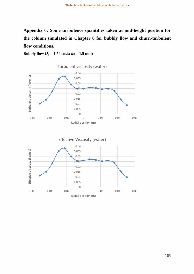
165
Appendix 6: Some turbulence quantities taken at mid-height position for
the column simulated in Chapter 6 for bubbly flow and churn-turbulent
flow conditions.
Bubbly flow (Jg = 1.54 cm/s; dB = 1.5 mm)
0
0,005
0,01
0,015
0,02
0,025
0,03
0,035
0,04
-0,06 -0,04 -0,02 0 0,02 0,04 0,06
Turb
ule
nt
Vis
cosi
ty (
kg/m
-s)
Radial position (m)
Turbulent viscosity (water)
0
0,005
0,01
0,015
0,02
0,025
0,03
0,035
0,04
-0,06 -0,04 -0,02 0 0,02 0,04 0,06
Effe
ctiv
e V
isco
sity
(kg
/m-s
)
Radial position (m)
Effective Viscosity (water)
Stellenbosch University https://scholar.sun.ac.za
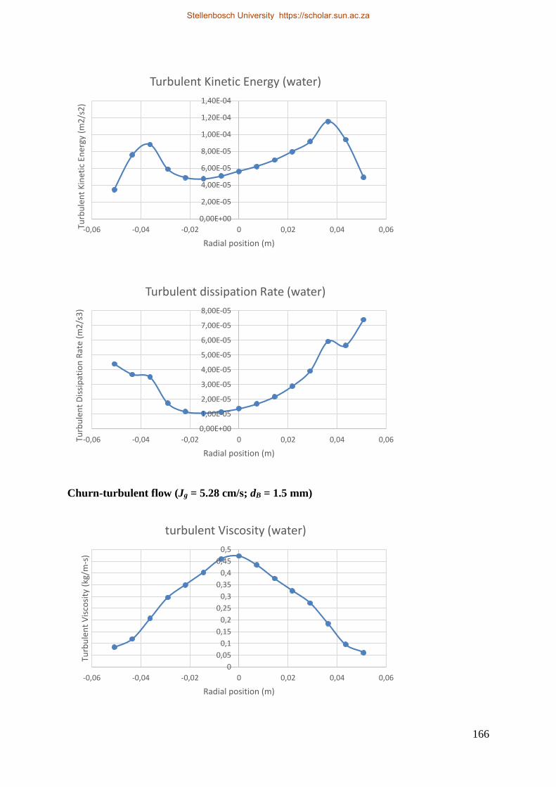
166
Churn-turbulent flow (Jg = 5.28 cm/s; dB = 1.5 mm)
0,00E+00
2,00E-05
4,00E-05
6,00E-05
8,00E-05
1,00E-04
1,20E-04
1,40E-04
-0,06 -0,04 -0,02 0 0,02 0,04 0,06Turb
ule
nt
Kin
etic
En
ergy
(m
2/s
2)
Radial position (m)
Turbulent Kinetic Energy (water)
0,00E+00
1,00E-05
2,00E-05
3,00E-05
4,00E-05
5,00E-05
6,00E-05
7,00E-05
8,00E-05
-0,06 -0,04 -0,02 0 0,02 0,04 0,06Turb
ule
nt
Dis
sip
atio
n R
ate
(m2
/s3
)
Radial position (m)
Turbulent dissipation Rate (water)
0
0,05
0,1
0,15
0,2
0,25
0,3
0,35
0,4
0,45
0,5
-0,06 -0,04 -0,02 0 0,02 0,04 0,06
Turb
ule
nt
Vis
cosi
ty (
kg/m
-s)
Radial position (m)
turbulent Viscosity (water)
Stellenbosch University https://scholar.sun.ac.za
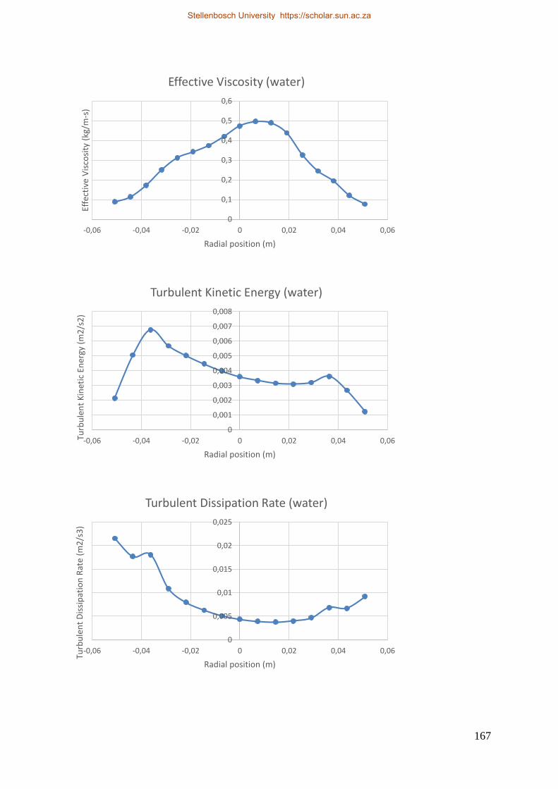
167
0
0,1
0,2
0,3
0,4
0,5
0,6
-0,06 -0,04 -0,02 0 0,02 0,04 0,06
Effe
ctiv
e V
isco
sity
(kg
/m-s
)
Radial position (m)
Effective Viscosity (water)
0
0,001
0,002
0,003
0,004
0,005
0,006
0,007
0,008
-0,06 -0,04 -0,02 0 0,02 0,04 0,06Turb
ule
nt
Kin
etic
En
ergy
(m
2/s
2)
Radial position (m)
Turbulent Kinetic Energy (water)
0
0,005
0,01
0,015
0,02
0,025
-0,06 -0,04 -0,02 0 0,02 0,04 0,06
Turb
ule
nt
Dis
sip
atio
n R
ate
(m2
/s3
)
Radial position (m)
Turbulent Dissipation Rate (water)
Stellenbosch University https://scholar.sun.ac.za