Embed Size (px)
Citation preview

One-dimensional modelling of mixing,dispersion and segregation of
multiphase fluids flowing in pipelines
by
Antonino Tomasello
A thesis submitted to Imperial College London in fulfilmentof the requirements for the degree of
Doctor of Philosophy
Department of Mechanical Engineering, Imperial College LondonExhibition Road, London SW7 2AZ
January 2009

To my sister

Abstract
The flow of immiscible liquids in pipelines has been studied in this work in order to formulate
a one-dimensional model for the computer analysis of two-phase liquid-liquid flow in horizontal
pipes. The model simplifies the number of flow patterns commonly encountered in liquid-liquid
flow to stratified flow, fully dispersed flow and partial dispersion with the formation of one or
two different emulsions. The model is based on the solution of continuity equations for dispersed
and continuous phase; correlations available in the literature are used for the calculation of the
maximum and mean dispersed phase drop diameter, the emulsion viscosity, the phase inversion
point, the liquid-wall friction factors, liquid-liquid friction factors at interface and the slip
velocity between the phases. In absence of validated models for entrainment and deposition
in liquid-liquid flow, two entrainment rate correlations and two deposition models originally
developed for gas-liquid flow have been adapted to liquid-liquid flow. The model was applied
to the flow of oil and water; the predicted flow regimes have been presented as a function
of the input water fraction and mixture velocity and compared with experimental results,
showing an overall good agreement between calculation and experiments. Calculated values
of oil-in-water and water-in-oil dispersed fractions were compared against experimental data
for different oil and water superficial velocities, input water fractions and mixture velocities.
Pressure losses calculated in the full developed flow region of the pipe, a crucial quantity in
industrial applications, are reasonably close to measured values. Discrepancies and possible
improvements of the model are also discussed.
The model for two-phase flow was extended to three-phase liquid-liquid-gas flow within
the framework of the two-fluid model. The two liquid phases were treated as a unique liquid
phase with properly averaged properties. The model for three-phase flow thus developed was
implemented in an existing research code for the simulation of three-phase slug flow with the
formation of emulsions in the liquid phase and phase inversion phenomena. Comparisons with
experimental data are presented.
3

Acknowledgements
This work has been undertaken under the Joint Project on Transient Multiphase Flows
TMF3. I wish to acknowledge the contributions made to this project by the Engineering and
Physical Sciences Research Council (EPSRC), the Department of Trade and Industry and the
following: Advantica; AspenTech; BP Exploration; Chevron; ConocoPhillips; ENI; ExxonMo-
bil; FEESA; Granherne / Subsea 7; Institutt for Energiteknikk; Institut Francais du Petrol;
Norsk Hydro; Petrobras; Scandpower; Shell; SINTEF; Statoil and Total. I wish to express my
sincere gratitude for this support.
I wish to express my deep gratitude to my supervisor, Dr R. I. Issa, for his guidance and
constant help and support. I am grateful I had the opportunity of benefitting from his knowl-
edge, his perspicacity and his experience in the complex and fascinating field of multiphase
flow. I would like to thank Professor G. F. Hewitt, whose wisdom and enthusiasm were an
inexhaustible source of inspiration both for the present work and for the whole TMF project.
I would like to thank Dr Colin Hale from the Chemical Engineering Department at Imperial
College, who provided the experimental data for two-phase and three-phase flow, together with
the knowledge we could share during our fruitful discussions.
My warmest thanks to my colleagues Silvere Barbeau, Bharat Lad and Marco Montini for
their friendship, their kind heart and for everything that I learnt from them. I wish them all
the best for their careers. Very many thanks also to all the PhD students I had the opportunity
to work with in room 503 at the Mechanical Engineering Department: I will not forget their
ability to create an entertaining atmosphere while working hard.
And I cannot forget all that my family did for me while I was so far from them and how
they managed to provide the encouragement and love I needed in many difficult moments. To
them, I am deeply in debt.
4

Contents
Abstract 3
Acknowledgements 4
List of figures 7
List of tables 15
Nomenclature 18
1 Introduction 27
1.1 Background . . . . . . . . . . . . . . . . . . . . . . . . . . . . . . . . . . . . . . . 27
1.2 Present contribution . . . . . . . . . . . . . . . . . . . . . . . . . . . . . . . . . . 28
1.3 Outline of the thesis . . . . . . . . . . . . . . . . . . . . . . . . . . . . . . . . . . 29
2 Literature review 33
2.1 Introduction . . . . . . . . . . . . . . . . . . . . . . . . . . . . . . . . . . . . . . . 33
2.2 Flow patterns in liquid-liquid flow . . . . . . . . . . . . . . . . . . . . . . . . . . 34
2.2.1 Factors influencing oil/water flow pattern . . . . . . . . . . . . . . . . . . 42
2.2.2 Interface curvature . . . . . . . . . . . . . . . . . . . . . . . . . . . . . . . 50
2.3 Pressure gradient and mixture viscosity . . . . . . . . . . . . . . . . . . . . . . . 54
2.4 Drop size and drop size distribution . . . . . . . . . . . . . . . . . . . . . . . . . 67
2.4.1 Drop size . . . . . . . . . . . . . . . . . . . . . . . . . . . . . . . . . . . . 67
2.4.2 Drop size distribution . . . . . . . . . . . . . . . . . . . . . . . . . . . . . 71
5

2.5 Drop breakup and coalescence . . . . . . . . . . . . . . . . . . . . . . . . . . . . . 73
2.5.1 Drop breakup and daughter drop size distribution . . . . . . . . . . . . . 74
2.5.2 Drops coalescence . . . . . . . . . . . . . . . . . . . . . . . . . . . . . . . 75
2.6 Secondary dispersion . . . . . . . . . . . . . . . . . . . . . . . . . . . . . . . . . . 76
2.7 Phase inversion . . . . . . . . . . . . . . . . . . . . . . . . . . . . . . . . . . . . . 78
2.7.1 Ambivalent emulsion region . . . . . . . . . . . . . . . . . . . . . . . . . . 79
2.7.2 Viscosity peak and pressure gradient in pipe flow . . . . . . . . . . . . . . 82
2.7.3 Prediction of phase inversion point . . . . . . . . . . . . . . . . . . . . . . 84
2.8 One-dimensional modelling of liquid-liquid and liquid-liquid-gas pipe flow . . . . 87
2.9 Summary . . . . . . . . . . . . . . . . . . . . . . . . . . . . . . . . . . . . . . . . 92
3 Present approach for liquid-liquid dispersions in pipelines 93
3.1 General description of the model . . . . . . . . . . . . . . . . . . . . . . . . . . . 93
3.2 Model equations . . . . . . . . . . . . . . . . . . . . . . . . . . . . . . . . . . . . 96
3.2.1 Closure models . . . . . . . . . . . . . . . . . . . . . . . . . . . . . . . . . 101
3.3 Entrainment models . . . . . . . . . . . . . . . . . . . . . . . . . . . . . . . . . . 107
3.3.1 Entrainment model based on de Bertodano et al. [1998] correlation . . . . 108
3.3.2 Entrainment rate based on Chesters and Issa [2004] model . . . . . . . . . 112
3.4 Deposition models . . . . . . . . . . . . . . . . . . . . . . . . . . . . . . . . . . . 117
3.4.1 Deposition model based on Zaichik and Alipchenkov [2001] . . . . . . . . 118
3.4.2 Deposition model based on Pan and Hanratty [2002] . . . . . . . . . . . . 123
4 Validation of the two-phase liquid-liquid model 129
4.1 Preamble . . . . . . . . . . . . . . . . . . . . . . . . . . . . . . . . . . . . . . . . 129
4.2 Dispersed phase fractions . . . . . . . . . . . . . . . . . . . . . . . . . . . . . . . 130
4.3 Flow regime maps . . . . . . . . . . . . . . . . . . . . . . . . . . . . . . . . . . . 139
4.4 Pressure losses . . . . . . . . . . . . . . . . . . . . . . . . . . . . . . . . . . . . . 147
4.4.1 Turbulence reduction due to dispersion of the phases - Effects on pressure
losses . . . . . . . . . . . . . . . . . . . . . . . . . . . . . . . . . . . . . . 162
4.5 Results obtained with the de Bertodano et al. [1998] correlation . . . . . . . . . . 176
4.6 Discussion . . . . . . . . . . . . . . . . . . . . . . . . . . . . . . . . . . . . . . . . 177
6

5 Three-phase oil/water/gas flow 181
5.1 Preamble . . . . . . . . . . . . . . . . . . . . . . . . . . . . . . . . . . . . . . . . 181
5.2 Equations for three-phase gas/liquid/liquid flow . . . . . . . . . . . . . . . . . . . 182
5.2.1 Closure models . . . . . . . . . . . . . . . . . . . . . . . . . . . . . . . . . 188
5.3 Dispersion model equations . . . . . . . . . . . . . . . . . . . . . . . . . . . . . . 191
5.4 Results . . . . . . . . . . . . . . . . . . . . . . . . . . . . . . . . . . . . . . . . . . 192
5.5 Conclusions . . . . . . . . . . . . . . . . . . . . . . . . . . . . . . . . . . . . . . . 198
6 Conclusions and future work 201
6.1 Conclusions . . . . . . . . . . . . . . . . . . . . . . . . . . . . . . . . . . . . . . . 201
6.2 Future work . . . . . . . . . . . . . . . . . . . . . . . . . . . . . . . . . . . . . . . 204
Bibliography 206
Appendix A. Hydrostatic pressure term for gas/liquid/liquid and liquid/liquid
flow 222
A-1 Hydrostatic pressure term for three-phase flow . . . . . . . . . . . . . . . . . . . 223
A-2 Hydrostatic pressure term for two-phase flow . . . . . . . . . . . . . . . . . . . . 226
Appendix B. Drift flux equations for liquid mixture 227
Appendix C. Results of the de Bertodano et al. [1998] correlation for en-
trainment rate 229
Appendix D. Model equations - Flowcharts of the solution procedure 241
7

8

List of Figures
2.1 Schematic of flow pattern for the 16.8 mPa s viscosity oil: (a) water velocity =
0.03 m/s; (b) water velocity = 0.20 m/s; (c) water velocity = 0.62 m/s; (from
Charles et al. [1961]) . . . . . . . . . . . . . . . . . . . . . . . . . . . . . . . . . . 35
2.2 Flow regimes for oil and water flow; oil density = 998 kg/m3 and: (a) oil viscosity
6.28 cP and 16.8 cP; (b) oil viscosity 65.0 cP (from Charles et al. [1961]) . . . . . 36
2.3 flow pattern at 20 cm (left) and 200 cm (right) from pipe inlet (from Hasson
et al. [1970]) . . . . . . . . . . . . . . . . . . . . . . . . . . . . . . . . . . . . . . . 38
2.4 Flow regimes identified and relative sketches in Arirachakaran et al. [1989] . . . . 39
2.5 Experimental flow maps for stainless steel pipe (a) and ’transpalite’ test section
(b) (from Angeli [1996]) . . . . . . . . . . . . . . . . . . . . . . . . . . . . . . . . 41
2.6 Experimental flow maps presented in Nadler and Mewes [1997]) . . . . . . . . . . 43
2.7 Experimental flow pattern map, 15upward, Scott [1985] (from Trallero [1995]) . 44
2.8 Experimental flow pattern map, -15downward, Cox [1985] (from Trallero [1995]) 44
2.9 Three-phase flow regime classification by Pan [1996] . . . . . . . . . . . . . . . . 45
2.10 (a) Observed water-gas flow patterns in inclined pipe; (b) Observed oil-water-gas
flow patterns in inclined pipe (Oddie et al. [2003]) . . . . . . . . . . . . . . . . . 46
2.11 Two-phase flow regimes identified by Hussain [2004] . . . . . . . . . . . . . . . . 50
2.12 Two phase flow configuration with curved interface (from Brauner et al. [1996]) . 51
2.13 Interface curvature (from Brauner et al. [1996]) . . . . . . . . . . . . . . . . . . . 52
2.14 Comparison between approximated constant curvature interface (dashed lines,
Brauner et al. [1996]) and exact solution (solid lines, Gorelik and Brauner [1999])
for wettability angle = 15 (from Gorelik and Brauner [1999]) . . . . . . . . . . . 53
9

2.15 Pressure gradient reduction factors as a function of interface position and per-
centage of water in the flowing stream (from Charles and Redberger [1962]) . . . 54
2.16 Pressure gradients for the oil of viscosity 6.29 cP as a function of the input
oil-water ratio and oil velocity. (Charles et al. [1961]) . . . . . . . . . . . . . . . . 55
2.17 Relative viscosity of suspensions of spheres - A, Einstein relation; B, curve for
spheres of very diverse sizes; C curve for spheres of equal size. Diamonds =
spheres of diverse sizes (Eilers [1941]); Circles = spheres of 17:1 size ratio (Ward
and Whitmore [1950]) - from Roscoe [1953] . . . . . . . . . . . . . . . . . . . . . 63
2.18 Comparison of van der Waarden [1954] data with Equations (2.16) and (2.17)
(from Pal and Rhodes [1989]) . . . . . . . . . . . . . . . . . . . . . . . . . . . . . 64
2.19 Measured relative viscosity versus Equation (2.19) (from Pal and Rhodes [1989]) 65
2.20 Drop size distribution of water in kerosene represented by a Rosin-Rammler type
of function (a) and an upper limit log-probability function (b) for U = 2.98 m/s
and 2.22 m/s (from Karabelas [1978]) . . . . . . . . . . . . . . . . . . . . . . . . 72
2.21 Phase inversion mechanism as in Laflin and Oglesby [1976] . . . . . . . . . . . . 79
2.22 Ambivalent range limits (from Selker and Sleicher [1965]) . . . . . . . . . . . . . 80
2.23 Region of ambivalence as affected by liquid/wall wetting, mixture velocity and
contact angle (Brauner and Ullmann [2002]) . . . . . . . . . . . . . . . . . . . . . 81
2.24 Mixture viscosity vs input water function (Arirachakaran et al. [1989]) . . . . . . 82
2.25 Pressure gradients reported in Soleimani [1999] . . . . . . . . . . . . . . . . . . . 83
2.26 Schematic of flow configuration in Vedapuri et al. [1997] (a) and Shi et al. [2002]
(b) (from Shi et al. [2002]) . . . . . . . . . . . . . . . . . . . . . . . . . . . . . . . 88
2.27 Three-phase slug flow. White = gas, Red = oil, Blue = water. (Bonizzi and Issa
[2003]) . . . . . . . . . . . . . . . . . . . . . . . . . . . . . . . . . . . . . . . . . . 91
3.1 Layers of oil in water and water in oil flowing inside a pipe . . . . . . . . . . . . 95
3.2 Entrainment and deposition scheme. Dw = water drops deposition, Ew = water
drops entrainment, Do = oil drops deposition, Eo = oil drops entrainment . . . . 96
3.3 Two phase flow variables . . . . . . . . . . . . . . . . . . . . . . . . . . . . . . . . 100
10

3.4 Slip velocity vs water cut at different mixture velocities, flat interface and pure
liquids . . . . . . . . . . . . . . . . . . . . . . . . . . . . . . . . . . . . . . . . . . 109
3.5 |us|+ c1|4u∗| vs inlet water cut at different mixture velocities, flat interface and
pure liquids. . . . . . . . . . . . . . . . . . . . . . . . . . . . . . . . . . . . . . . . 111
3.6 Water in oil and oil in water entrainment rates for different mixture velocities
and input water fractions from de Bertodano et al. [1998] correlation . . . . . . . 112
3.7 Pinch-off at phase inversion front (Chesters and Issa [2004]) . . . . . . . . . . . . 113
3.8 Experimental root mean square velocity profiles for different mixture velocities,
normalized with the friction velocity. (Elseth [2001]) . . . . . . . . . . . . . . . . 115
3.9 Water in oil and oil in water entrainment rates for different mixture velocities
and input water fractions from Chesters and Issa [2004] correlation . . . . . . . . 117
3.10 Elasticity parameter e as a function of drop diameter for different mixture velocities121
3.11 Water deposition rate predicted by Equations (3.68) (black line) and (3.71) (red
line) for drop diameter = 1 mm, 2 mm, 3 mm and 4 mm respectively. Dispersed
phase fraction = 50%. . . . . . . . . . . . . . . . . . . . . . . . . . . . . . . . . . 125
3.12 Oil deposition rate predicted by Equations (3.68) (black line) and (3.72) (red
line) for drop diameter = 1 mm, 2 mm, 3 mm and 4 mm respectively. Dispersed
phase fraction = 50%. . . . . . . . . . . . . . . . . . . . . . . . . . . . . . . . . . 126
4.1 Measured and predicted entrained oil fraction in water continuous phase for oil
superficial velocities 0.35 m/s and 0.8 m/s (experiments by Al-Wahaibi [2006]) . 131
4.2 Measured and predicted entrained water fraction in oil continuous phase for oil
superficial velocities 0.35 m/s and 0.8 m/s (experiments by Al-Wahaibi [2006]) . 132
4.3 Measured and predicted entrained oil fraction in water continuous phase for oil
superficial velocities 1.1 m/s and 1.4 m/s (experiments by Al-Wahaibi [2006]) . . 133
4.4 Measured and predicted entrained water fraction in oil continuous phase for oil
superficial velocities 1.1 m/s and 1.4 m/s (experiments by Al-Wahaibi [2006]) . . 133
4.5 Oil fraction dispersed into water for uM = 1.34 and uM = 1.5. (Elseth [2001]) . . 135
4.6 Oil fraction dispersed into water for uM = 1.67 and uM = 2.0. (Elseth [2001]) . . 136
4.7 Oil fraction dispersed into water for uM = 2.5 and uM = 3.0. (Elseth [2001]) . . 136
11

4.8 Water fraction dispersed into oil for uM = 1.34 and uM = 1.5. (Elseth [2001]) . . 137
4.9 Water fraction dispersed into oil for uM = 1.67 and uM = 2.0. (Elseth [2001]) . . 137
4.10 Water fraction dispersed into oil for uM = 2.5 and uM = 3.0. (Elseth [2001]) . . 138
4.11 Dispersed phase fractions (Soleimani [1999]). UM = 1.25 m/s . . . . . . . . . . . 140
4.12 Dispersed phase fractions (Lovick [2004]) . . . . . . . . . . . . . . . . . . . . . . . 140
4.13 Dispersed phase fractions (Lovick [2004]) . . . . . . . . . . . . . . . . . . . . . . . 141
4.14 Flow patterns (Elseth [2001]) . . . . . . . . . . . . . . . . . . . . . . . . . . . . . 142
4.15 Experimental flow map (Elseth [2001]) and model predictions . . . . . . . . . . . 143
4.16 Flow patterns (Hussain [2004]) . . . . . . . . . . . . . . . . . . . . . . . . . . . . 146
4.17 Measured and predicted pressure losses for pure water (a) and pure oil (b) (Hus-
sain [2004]) . . . . . . . . . . . . . . . . . . . . . . . . . . . . . . . . . . . . . . . 148
4.18 Calculated and measured pressure losses (experimental data by Hussain [2004])
- Hand correlation . . . . . . . . . . . . . . . . . . . . . . . . . . . . . . . . . . . 149
4.19 Measured pressure gradient as a function of distance from inlet (Hussain [2004]) 150
4.20 Pressure losses by Hussain [2004] - Blasius correlation . . . . . . . . . . . . . . . 151
4.21 Pressure losses by Hussain [2004] - Zigrang & Sylvester correlation . . . . . . . . 152
4.22 Measured and predicted pressure losses for pure water (a) and pure oil (b)
(Soleimani [1999]) . . . . . . . . . . . . . . . . . . . . . . . . . . . . . . . . . . . 153
4.23 Pressure losses by Soleimani [1999] - low mixture velocities - Hand correlation . . 154
4.24 Pressure losses by Soleimani [1999] - high mixture velocities - Hand correlation . 154
4.25 Pressure losses by Soleimani [1999] - Blasius correlation . . . . . . . . . . . . . . 156
4.26 Pressure losses by Soleimani [1999] - Zigrang & Sylvester correlation . . . . . . . 156
4.27 Measured and predicted pressure losses for pure water (a) and pure oil (b) (Elseth
[2001]) . . . . . . . . . . . . . . . . . . . . . . . . . . . . . . . . . . . . . . . . . . 157
4.28 Measured and predicted pressure losses with Hand correlation (experimental data
by Elseth [2001]) . . . . . . . . . . . . . . . . . . . . . . . . . . . . . . . . . . . . 158
4.29 Measured and predicted pressure losses with Blasius correlation (experimental
data by Elseth [2001]) . . . . . . . . . . . . . . . . . . . . . . . . . . . . . . . . . 158
4.30 Measured and predicted pressure losses with Zigrang & Sylvester correlation
(experimental data by Elseth [2001]) . . . . . . . . . . . . . . . . . . . . . . . . . 159
12

4.31 Measured and predicted pressure losses for pure water (a) and pure oil (b) (Lovick
[2004]) . . . . . . . . . . . . . . . . . . . . . . . . . . . . . . . . . . . . . . . . . . 160
4.32 Measured and predicted pressure losses - Hand correlation (Lovick [2004]) . . . . 161
4.33 Measured and predicted pressure losses - Blasius correlation (Lovick [2004]) . . . 161
4.34 Measured and predicted pressure losses - Zigrang & Sylvester correlation (Lovick
[2004]) . . . . . . . . . . . . . . . . . . . . . . . . . . . . . . . . . . . . . . . . . . 162
4.35 Friction factors for unstable oil-in-water and water-in-oil dispersions (Pal [1993]) 163
4.36 Soleimani’s data against correlation available and homogeneous model - mixture
velocity = 3.0 m/s . . . . . . . . . . . . . . . . . . . . . . . . . . . . . . . . . . . 164
4.37 Pressure losses at 3.0 m/s with turbulence damping - experimental data from
Soleimani [1999] . . . . . . . . . . . . . . . . . . . . . . . . . . . . . . . . . . . . 166
4.38 Pressure losses at 3.0 m/s with turbulence damping - predictions of Hand’s cor-
relation against experimental data from Soleimani [1999] . . . . . . . . . . . . . . 166
4.39 Pressure gradient calculated with turbulence damping according to Rozentsvaig
[1982] and Hand correlation (experimental data by Soleimani [1999]) . . . . . . . 167
4.40 Pressure gradient calculated with turbulence damping according to Rozentsvaig
[1982] and Blasius correlation (experimental data by Soleimani [1999]) . . . . . . 169
4.41 Pressure losses (Elseth [2001]) . . . . . . . . . . . . . . . . . . . . . . . . . . . . . 171
4.42 Relative viscosity for emulsions with λµ < 1 (a) and λµ > 1 (b) (Pal [2007]) . . . 173
4.43 Relative viscosity for water-in-oil (a) and oil-in-water (b) emulsions from Equa-
tions (4.13) and (4.14) - Fluids properties as in Soleimani [1999] . . . . . . . . . 174
4.44 Pressure gradient measured by Soleimani compared with the prediction of Equa-
tion (4.14) with φm = 0.5 for water in oil dispersions and φm = 0.74 for oil in
water dispersions. . . . . . . . . . . . . . . . . . . . . . . . . . . . . . . . . . . . . 175
5.1 Three-phase flow model variables . . . . . . . . . . . . . . . . . . . . . . . . . . . 183
5.2 Graphic representation of the calculated distribution of oil and water inside the
pipe. UL = 0.5 m/s, UG = 4.0 m/s, water cut = 0.4 - Present model . . . . . . . 193
13

5.3 Graphic representation of the calculated distribution of oil and water inside the
pipe. UL = 0.5 m/s, UG = 4.0 m/s, water cut = 0.4 - Model by Bonizzi and Issa
[2003] . . . . . . . . . . . . . . . . . . . . . . . . . . . . . . . . . . . . . . . . . . 193
5.4 Three-phase flow pressure losses. Experimental data by Odozi [2000] . . . . . . . 194
5.5 Average fully dispersed fraction inside the dispersed slug body (analytical data,
Odozi [2000] experiments) . . . . . . . . . . . . . . . . . . . . . . . . . . . . . . . 196
5.6 Experimental and calculated slug frequency . . . . . . . . . . . . . . . . . . . . . 197
5.7 Calculated and experimental slug translational velocity . . . . . . . . . . . . . . . 198
A-1 Hydrostatic pressure inside the liquid phases . . . . . . . . . . . . . . . . . . . . 223
C-1 Oil fraction dispersed in water for oil superficial velocities Uso = 1.1 m/s and
Uso = 1.4 m/s (Al-Wahaibi [2006]) . . . . . . . . . . . . . . . . . . . . . . . . . . 229
C-2 Water fraction dispersed in oil for oil superficial velocities Uso = 1.1 m/s and
Uso = 1.4 m/s (Al-Wahaibi [2006]) . . . . . . . . . . . . . . . . . . . . . . . . . . 230
C-3 Oil fraction dispersed in water for UM = 1.34 m/s and UM = 1.5 m/s (Elseth
[2001]) . . . . . . . . . . . . . . . . . . . . . . . . . . . . . . . . . . . . . . . . . . 230
C-4 Oil fraction dispersed in water for UM = 1.67 m/s and UM = 2.0 m/s (Elseth
[2001]) . . . . . . . . . . . . . . . . . . . . . . . . . . . . . . . . . . . . . . . . . . 231
C-5 Oil fraction dispersed in water for UM = 2.5 m/s and UM = 3.0 m/s (Elseth
[2001]) . . . . . . . . . . . . . . . . . . . . . . . . . . . . . . . . . . . . . . . . . . 231
C-6 Water fraction dispersed in oil for UM = 1.34 m/s and UM = 1.5 m/s (Elseth
[2001]) . . . . . . . . . . . . . . . . . . . . . . . . . . . . . . . . . . . . . . . . . . 232
C-7 Water fraction dispersed in oil for UM = 1.67 m/s and UM = 2.0 m/s (Elseth
[2001]) . . . . . . . . . . . . . . . . . . . . . . . . . . . . . . . . . . . . . . . . . . 232
C-8 Water fraction dispersed in oil for UM = 2.5 m/s and UM = 3.0 m/s (Elseth
[2001]) . . . . . . . . . . . . . . . . . . . . . . . . . . . . . . . . . . . . . . . . . . 233
C-9 Dispersed phase fractions - data by Soleimani [1999]. UM = 1.25 m/s . . . . . . . 233
C-10 Dispersed phase fractions UM = 1.0 m/s - data by Lovick [2004] . . . . . . . . . 234
C-11 Dispersed phase fractions UM = 1.5 m/s - data by Lovick [2004] . . . . . . . . . 234
C-12 Pressure losses by Hussain [2004] - Hand correlation . . . . . . . . . . . . . . . . 235
14

C-13 Pressure losses by Hussain [2004] - Blasius correlation . . . . . . . . . . . . . . . 235
C-14 Pressure losses by Hussain [2004] - Zigrang & Sylvester correlation . . . . . . . . 236
C-15 Pressure losses by Soleimani [1999] - Hand correlation . . . . . . . . . . . . . . . 236
C-16 Pressure losses by Soleimani [1999] - Blasius correlation . . . . . . . . . . . . . . 237
C-17 Pressure losses by Soleimani [1999] - Zigrang & Sylvester correlation . . . . . . . 238
C-18 Pressure losses by Elseth [2001] - Hand correlation . . . . . . . . . . . . . . . . . 239
C-19 Pressure losses by Elseth [2001] - Blasius correlation . . . . . . . . . . . . . . . . 240
C-20 Pressure losses by Elseth [2001] - Zigrang & Sylvester correlation . . . . . . . . . 240
D-1 Model for dispersion and segregation of the phases: explicit solution scheme with
layer velocities calculated from the mixture velocity uM and the slip velocity us . 241
D-2 Model for dispersion and segregation of the phases: implicit solution scheme with
solution of the momentum equations for the layers velocities. . . . . . . . . . . . 242
15

16

List of Tables
2.1 Flow pattern classification according to Trallero [1995] . . . . . . . . . . . . . . . 41
2.2 Relation between the flow pattern classification of Angeli [1996] and Trallero
[1995] proposed by Valle [2000] . . . . . . . . . . . . . . . . . . . . . . . . . . . . 42
2.3 Influence of pipe material on flow patterns identified by Angeli and Hewitt [2000b] 48
4.1 Fluids properties and pipe geometry for Al-Wahaibi [2006] experiments . . . . . 131
4.2 Fluids properties and pipe geometry for Elseth [2001] experiments . . . . . . . . 135
4.3 Errors between data by Elseth [2001] and predictions . . . . . . . . . . . . . . . . 139
4.4 Elseth [2001] flow patterns reclassified . . . . . . . . . . . . . . . . . . . . . . . . 141
4.5 Criteria used to match experimental flow patterns and predictions. (Experiments
by Elseth [2001]) . . . . . . . . . . . . . . . . . . . . . . . . . . . . . . . . . . . . 142
4.6 Fluids properties and pipe geometry for Hussain [2004] experiments . . . . . . . 145
4.7 Hussain [2004] flow patterns reclassified . . . . . . . . . . . . . . . . . . . . . . . 146
4.8 AAE and AAAE for data reported in Figure 4.18 . . . . . . . . . . . . . . . . . . 149
4.9 AAE and AAAE for data reported in Figure 4.20 . . . . . . . . . . . . . . . . . . 151
4.10 AAE and AAAE for data reported in Figure 4.21 . . . . . . . . . . . . . . . . . . 152
4.11 AAE and AAAE for data reported in Figures 4.23 and 4.24 . . . . . . . . . . . . 155
4.12 AAE and AAAE for data reported in Figures 4.25 and 4.26 . . . . . . . . . . . . 155
4.13 AAE and AAAE for pressure losses measured by Elseth [2001] . . . . . . . . . . 159
4.14 AAE and AAAE for pressure losses measured by Lovick [2004] . . . . . . . . . . 160
17

4.15 Errors for pressure losses calculated with turbulence reduction (Figure 4.39).
Comparison with the errors presented without turbulence reduction (Figures
4.23 and 4.24) . . . . . . . . . . . . . . . . . . . . . . . . . . . . . . . . . . . . . . 167
4.16 Errors for pressure losses calculated with turbulence reduction (Figure 4.40).
Comparison with the errors presented without turbulence reduction (Figure 4.25) 169
4.17 Errors for pressure losses calculated with turbulence reduction (Figure 4.41).
Comparison with the errors presented without turbulence reduction (Figures
4.28 and 4.29). d. r. = drag reduction correlation. . . . . . . . . . . . . . . . . . 170
5.1 Fluids properties and pipe geometry for Odozi [2000] experiments . . . . . . . . . 192
18

Nomenclature
Roman letters
A Cross section area[m2
]
Ad Parameter in Equation (3.63) [−]
AH Parameter in Equation (3.64) [−]
Ai Interfacial area[m2
]
CD Drag coefficient [−]
CE Parameter in Equation (3.44) ≈ 9.8 [−]
Ck Crowding factor in Equation (2.14) [−]
cl Lower layer fraction [−]
Csubscript General form of parameters and constants [−]
Cµ Empirical coefficient in k − ε model = 0.09 [−]
Cη
Parameter in drag reduction model by Rozentsvaig
[1982][−]
Ct Turbulent response function [−]
Cvm Virtual mass coefficient [−]
cw Water cut [−]
D Pipe diameter [m]
Dk Hydraulic diameter - phase k [m]
d Drop diameter [m]
d32 Mean Sauter diameter [m]
19

E, Ep, Es Energy, potential energy, surface energy [J ]
Eo/w Percentage of oil dispersed in water [−]
Ew/o Percentage of water dispersed in oil [−]
e Elasticity parameter for drop collisions [−]
er Wall roughness [m]
eT Parameter in Equation (2.6) [−]
Fi Liquid-liquid interfacial force per unit volume[N/m3
]
Fj Liquid-gas interfacial force per unit volume[N/m3
]
FWL Liquid-wall force term per unit volume[N/m3
]
f Friction factor [−]
g Gravity acceleration[m/s2
]
H Parameter in Equation (3.57) []
h Distance from bottom of the pipe [m]
Jd Deposition rate[kg/(m2s)
]
Jg Deposition rate - gravity contribution[kg/(m2s)
]
Jt Deposition rate - turbulent contribution[kg/(m2s)
]
k Turbulent kinetic energy[m2/s2
]
L Length [m]
Ld Characteristic dimension of a drop [m]
le Eddy length scale [m]
M Mass flow rate [kg/s]
Nwaves Number of interfacial waves in a control volume [−]
n, n1, n2 Generic exponent [−]
P Turbulent energy production rate[m2/s3
]
p Pressure [Pa]
pi Pressure at liquid-liquid interface [Pa]
pj Pressure at gas-liquid interface [Pa]
20

p (w) Probability of event w [−]
Q Volumetric flow rate[m3/s
]
R Pipe radius [m]
RE Entrainment rate[kg/(m2s)
]
Sk Wetted perimeter - phase/layer k [m]
Sλ Source term for phase λ[kg/(m3s)
]
s Solid surface area per unit volume[m−1
]
T Temperature [K]
TL Lagrangian timescale [s]
TLp Eddy-particle interaction time [s]
t Time [s]
U Superficial velocity [m/s]
u Velocity [m/s]
ub Bulk velocity [m/s]
us Slip velocity [m/s]
uT Dispersed drop terminal velocity [m/s]
u∗ Friction velocity [m/s]
u+ Dimensionless velocity [−]
u′ Fluctuating velocity component (continuous phase) [m/s]
v′ Fluctuating velocity component (dispersed phase) [m/s]
V Cumulative volume fraction [−]
Vd Drops deposition velocity [m/s]
vp Drop deposition velocity due to turbulence [m/s]
X Parameter in Equation 2.5 [−]
y+ Dimensionless distance from pipe wall [−]
z Parameter in Equation (2.41) [−]
21

Dimensionless numbers
Eo Eotvos number
NV i Viscosity group in Equation (2.31)
NCa Capillary number
Re Reynolds number
Red Particle Reynolds number
We Weber number
Wet Turbulent Weber number
Greek letters
αo Oil fraction in the upper layer [−]
αw Water fraction in the bottom layer [−]
βo Oil fraction in the bottom layer [−]
βt Parameter in Equation (3.63) [−]
βw Water fraction in the upper layer [−]
γ Pipe inclination [rad]
δExperimental parameter in upper limit log-
probability drop size distribution[−]
δt
Dispersed phase fraction threshold between stratified
and partially dispersed flow[−]
δw Water film thickness in water/gas annular flow [m]
ε Turbulent energy dissipation rate[m2/s3
]
ζExperimental parameter in upper limit log-
probability drop size distribution[−]
θ Wettability angle [rad]
ϑi Liquid-liquid interfacial angle [rad]
ϑj Gas-liquid interfacial angle [rad]
κ Von Karman’s constant = 0.41 [−]
22

λ Wavelength [m]
λij Crowding factor for polydisperse systems [−]
λµ Viscosity ratio = µd/µc [−]
λw Water fraction at phase inversion point [−]
µ Dynamic viscosity [Pa s]
µr Relative mixture viscosity = µM/µc [−]
ν Kinematic viscosity[m2/s
]
ρ Density[kg/m3
]
σ Surface tension [N/m]
σp Standard deviation [−]
τ Shear stress [Pa]
τcl Intercollision time [s]
τdef Drop deformation time [s]
τdris Drop disintegration time [s]
τE Characteristic entrainment time [s]
τp Particle response time [s]
τpinch−off Pinch-off time [s]
Υk Generic function of phase k []
Φ Parameter in Equation 2.5 [−]
φ Dispersed phase concentration [−]
φm Drops maximum packing volume fraction [−]
φ2x, φ2
r, φ2ϕ Restitution coefficients [−]
φ0, φ∗, φp0 Angles in Equation (2.1) and Figure 2.12 [−]
χ Rebound coefficient [−]
ΨAdditional hydrostatic pressure term in liquid mo-
mentum equation
[N/m3
]
Ω Term in liquid momentum equation[N/m3
]
23

Subscripts
0 dilute dispersion
ε dense dispersion
ϕ tangential direction
c continuous
crit critical
D drag
d dispersed
E entrainment
g gas phase
i interface (upper layer-lower layer)
j interface (gas-upper layer)
k generic phase
k faster phase
L liquid
l lower layer
M mixture
max maximum
o oil
otM oil at total mixture flow rate
o/w oil in water
r radial direction
TP two-phase
u upper layer
W wall
w water
w/g water/gas
24

w/o water in oil
wtM water at total mixture flow rate
x axial direction
Abbreviations
1D One-Dimension
3D Three-Dimension
AAE Arithmetic Average Error
AAAE Arithmetic Absolute Average Error
CFD Computational Fluid Dynamics
HAAE Harmonic Absolute Average Error
LHS Left Hand Side
RHS Right Hand Side
r.m.s. root mean square
25

26

Chapter 1
Introduction
1.1 Background
Transport of heavy crude oil over long distances through pipelines may be expensive due
the relatively high viscosity of the fluid and, consequently, to the considerable pumping power
required. Attempts have been made to reduce the viscosity of the transported oil by increas-
ing its temperature; however, the cost of heating long pipelines makes the application of this
technique not effective. Another simple approach to reduce the pressure loss in oil pipelines
consists in the addition of an immiscible, less viscous phase. In the case of oil transport, water
is the ideal additional fluid for its low cost, its abundance and because separation of the two
fluids at the end at the pipeline is a relatively easy and cheap process. To reduce the shear
stress between the fluids and the internal wall of the pipe, it is desirable that the less viscous
fluid wets the wall while keeping the more viscous fluid confined in the core of the pipe. This is
achieved with oil and water flowing in annular configuration with water in the external annulus.
A small amount of water can be sufficient to yield significant pressure loss reduction. Unfor-
tunately, creating and sustaining liquid-liquid annular flow over long distances is not an easy
task as the equilibrium between the phases can be disrupted by buoyancy forces, entrainment
between the phases and irregularity in the pipeline, such as bends, valves and junctions. In
general, annular flow is seldom achieved and the distribution of the phases inside the pipeline
27

is complex and characterised by many different flow patterns, each with its own hydrodynamic
properties. For horizontal pipes and when the fluids have large differences in density, the flow
is often segregated with the lighter fluid flowing on top of the heavier one. For larger mixture
velocities dispersion occurs and emulsions are formed. It has been observed that emulsions
with oil as the continuous phase and a small amount of water as the dispersed phase give rise
to smaller pressure losses than those of pure oil. Obviously, the formation of an emulsion of
water dispersed in oil is much easier to obtain and keep stable than oil-core annular flow. The
concentration of the dispersed water is, in general, not constant in time or along the pipe, nor
uniform across the pipe section. The variation of concentration of the dispersed water and the
interaction between the dispersed drops among themselves and with the continuous phase can
produce local phase inversion. When this happens, an oil continuous mixture becomes a water
continuous mixture, with a change in the hydrodynamic properties of the emulsion. Prediction
and control of the flow pattern and its hydrodynamic properties are the first steps for the design
of the pumping systems and the separators at the end of the pipeline.
Pipelines are commonly studied with one-dimensional models since two- and three-dimensional
methods can be very expensive in terms of computing resources and time, considering the length
of the pipelines. A few models have been proposed in the past for the one-dimensional analyt-
ical description of two-phase liquid/liquid and three-phase liquid/liquid/gas flow in pipelines.
Different approximations have been used to account for the momentum exchange between the
phases and the formation of emulsions. In particular, the prediction of the formation of emul-
sions, the flow pattern and phase inversion are often sources of inaccuracy for these models.
1.2 Present contribution
The present work aims at making a contribution to the study of segregated and dispersed
flows of two immiscible liquids in pipelines. The objective of the study is to provide a simple
tool for the prediction of the formation of emulsions in two-phase liquid/liquid flow in horizontal
pipes. The tasks undertaken can be summarized as follows:
• A framework of the model is first elaborated in order to reduce the complexity of two-
phase liquid/liquid flow to a scheme easy enough to be implemented in a one-dimensional,
28

Eulerian computer code;
• A set of equations is formulated, whose solution provides a quantitative measure of the
dispersion of the two fluids as they flow along the pipeline;
• The closure models required by the equations of the model are selected, namely mass ex-
change terms accounting for the formation of dispersed drops, liquid-wall and liquid-liquid
friction factors, phase inversion point correlations, dispersed phase drop diameter. In the
present work, the mass exchange terms required special modelling with the introduction
of entrainment and deposition rate closure;
• The model is then validated against experimental data.
1.3 Outline of the thesis
Chapter 2 offers a brief overview of the main features of the flow of two immiscible liquids
in a pipeline. Attention is paid to the flow pattern usually identified in liquid-liquid flow
because of the great effect that the flow pattern has on the pressure drop. The literature
on pressure drop is then examined in detail together with several correlations proposed for
the calculation of the mixture viscosity when dispersion occurs. The focus then moves to the
theoretical formulation of the mechanism responsible for drop fragmentation and how analytical
expressions for the maximum drop diameter in turbulent flow are derived. The hypothesis of
flat drop size distribution is adopted in the present work and the expression by Brauner [2001]
is selected for the calculations. A section of the literature review is dedicated to phase inversion,
usually associated with large and rapid changes in the mixture viscosity and pressure losses.
The prediction of the phase inversion point is a key point in liquid-liquid flow as it involves
dramatic changes in the mixture properties. Despite its relevant effects, phase inversion in
pipelines has received less attention in the research field than phase inversion in stirred tanks.
As a consequence, the current understanding of the mechanisms involved is not accurate and
a relatively small number of correlations for the phase inversion point in pipelines is available.
In this study, the correlations by Decarre and Fabre [1997] are adopted, although they were
originally proposed for agitated vessels. Finally, a brief overview of the available numerical
29

models for two and three-phase flow is presented.
Chapter 3 presents the proposed approach to the simulation of liquid-liquid flow. A sim-
ple set of equations is presented to describe the evolution of the dispersed phase fractions in
space and time. Closure models are presented for the formation of emulsions, in the form of
entrainment and deposition models. At the interface between the fluids waves can appear from
which drops are entrained forming emulsions. The detailed mechanism of formation of drops
is complex and involves complex analytical tools. In this study, however, the mechanism of
entrainment is related to bulk flow quantities through non-dimensional numbers through two
entrainment models, those of Chesters and Issa [2004] and of de Bertodano et al. [1998]. The
second mass exchange term considered is the deposition term, related to the contribution of
gravity and continuous phase turbulence. Two deposition models (Zaichik and Alipchenkov
[2001] and Pan and Hanratty [2002]) are presented in the chapter; coupling together one en-
trainment model with one deposition model allows the equations of the dispersion-segregation
model to simulate the formation of either emulsions or of stratified flow within the flow patterns
accounted for by the model.
Chapter 4 compares the results of the model against different sets of experimental data.
Attention is focused on the dispersed phase fractions, flow patterns and pressure losses. A
critical factor in the calculation of the pressure losses in turbulent dispersed flow is the effect
of the dispersed phase on the continuous phase turbulence: when dispersed drops reduce the
continuous phase turbulence, the resulting pressure losses are less than those measured for the
continuous phase flowing alone at the same velocity. The effects of the dispersed phase on the
continuous phase turbulence has not been addressed by researchers in liquid-liquid flow in as
much detail as in gas-liquid flow and there are few models for the pressure losses in liquid-liquid
flow. A simple relation for drag reduction (Rozentsvaig [1982]) is used to compare results on
pressure losses with and without drag reduction.
Chapter 5 illustrates the possibility of using the dispersion model described in Chapter 3
to three-phase gas/liquid/liquid flow in horizontal pipes and presents some preliminary results.
In particular, three-phase slug flow is the object of study and the model is implemented within
the research computer code TRIOMPH. Three-phase slug flow is a complex flow involving both
a gas-liquid interface and a liquid-liquid interface. Waves at the gas-liquid interface may grow
30

becoming slugs: the coupling of the dispersion model with the TRIOMPH code accounts for the
changes in the composition of the liquid mass (formation of emulsions or stratification) both in
the slug body and in the liquid film between two consecutive slugs. The implementation and
validation of the model for three-phase flow presented is in its early stage and more work is left
for future studies.
Chapter 6 presents the conclusions reached by this study together with suggestions for
future work that might be undertaken to improve the current model.
31

32

Chapter 2
Literature review
2.1 Introduction
In this chapter previous work on two-phase liquid-liquid flow is briefly reviewed, focusing
attention on oil/water flow. The first topic covered in the chapter is the different flow patterns
observed in experimental work and the classifications proposed to group the observed flow
patterns (section 2.2). Factors influencing the flow pattern are discussed (section 2.2.1) together
with the literature on the interface curvature evaluation (section 2.2.2). Section 2.3 is dedicated
to an important parameter in industrial two-phase flows applications, namely the pressure
gradient. A relevant aspect in the calculation of the pressure gradient is the mixture viscosity
of the emulsion flowing in the pipe; models for emulsion viscosity are reported in the same
section. There follows an exposition of the studies on the dispersed phase drop size and drop
size distribution (section 2.4), drop breakup and coalescence (section 2.5) and formation of
secondary dispersion (section 2.6). Section 2.7 discusses the phase inversion phenomenon and
the criteria to predict phase inversion. The chapter is concluded with a section (2.8) dedicated
to one-dimensional CFD models available in the literature for two-phase immiscible flow in
pipelines.
33

2.2 Flow patterns in liquid-liquid flow
Two or more phases flowing inside a pipeline may assume different geometrical flow config-
urations, referred to as flow patterns. The recognition of the flow pattern inside a pipe is of
great relevance since many characteristic flow quantities (such as pressure losses) are strongly
influenced by the flow pattern.
Experimentalists have proposed a classification of the flow patterns observed for liquid-
liquid flow according to the interface distribution and the in-situ phase fraction. The onset
of a particular flow pattern is governed by the interaction of the fluid physical properties and
the flow parameters; therefore the actual flow pattern is determined mainly by fluid fractions,
fluid viscosities and densities, fluid superficial velocities and interfacial properties, wettability
and geometry of the pipe (internal diameter, inclination, inlet section shape and presence or
absence of mixers at inlet).
The present work focuses on immiscible fluids flowing in horizontal and slightly inclined
pipes. The flow patterns encountered in horizontal pipes are more complex than those observed
in vertical pipes, mainly due to the effect of gravity and buoyancy that tend to separate the
fluids, with the lighter phase flowing on top of the heavier one.
Russel et al. [1959] performed experiments to investigate the flow characteristics of a white
mineral oil and water in a horizontal smooth pipe. The oil had a viscosity of 18.0 mPa s at 25
C and a density of 834 kg/m3. A smooth transparent 25.4 mm diameter horizontal pipe was
used while the oil-water volume flow rate ratio ranged from 0.1 to 10 and the water velocity
varied from 0.035 m/s to 1.08 m/s. Attention was paid to the measurement of pressure drop
and observation of the flow pattern. It was found that at low flow rates a quiescent interface
existed between the oil and water streams, while at high flow rates the interface tended to break
up. As the mixed flow pattern is approached, the interface becomes increasingly wavy.
Similar experiments were conducted by Charles et al. [1961], who used a 1-inch diameter
laboratory pipeline and different oils. They observed a similar series of flow patterns for each
oil and the flow patterns were found to be largely independent of the oil viscosity. At high
oil-water ratios, oil formed the continuous phase with dispersed water drops. As the oil-water
ratio was decreased, four flow patterns were observed: concentric oil-in-water, oil-slugs-in-water,
34

oil-drops-in-water and oil drops in continuous water. Anomalies were exhibited by the most
viscous oil at low superficial water velocities and this was attributed by the authors to the
interfacial properties and the interface energy, which cannot be neglected for low kinetic energy
flows. Annular flow was observed only in the form of water-annulus/oil core while oil-annulus
annular flow was never observed. Charles et al. [1961] attempted to correlate their experimental
findings to those of Russel et al. [1959] and, in particular, they observed that the bubble flow of
Russel et al. appeared to correspond to their oil-drops-in-water, oil-bubbles-in-water and oil-
slugs-in-water flow patterns while the stratified flow pattern and the mixed flow were related
by Charles et al. to the concentric oil-in-water flow pattern and to the water-in-oil flow pattern
respectively.
Figures 2.1 and 2.2 reproduce the flow pattern classification and the flow maps presented
by Charles et al. [1961].
(a) (b)
(c)
Figure 2.1: Schematic of flow pattern for the 16.8 mPa s viscosity oil: (a) water velocity = 0.03m/s; (b) water velocity = 0.20 m/s; (c) water velocity = 0.62 m/s; (from Charles et al. [1961])
The maps in Figure 2.2 show that for low oil and water velocities only partial dispersion is
achieved. On the other hand, totally dispersed flow is obtained when the velocity of one of the
35

(a) (b)
Figure 2.2: Flow regimes for oil and water flow; oil density = 998 kg/m3 and: (a) oil viscosity6.28 cP and 16.8 cP; (b) oil viscosity 65.0 cP (from Charles et al. [1961])
36

phases is significantly higher than the other phase. Although the two maps summarize results
obtained for oils whose viscosities are significantly different, they show a very similar behaviour
for the two liquid phases.
Hasson et al. [1970] performed a study of the flow mechanisms of two immiscible liquids, with
a small density difference, introduced at a horizontal pipe inlet in a concentric flow pattern. The
aim of the study was the investigation of the extent of the annular flow, its break-up mechanisms
and the subsequent flow pattern produced. The two immiscible liquids were distilled water and a
kerosene-perchlorethylene solution, mixed together to give a mixture with density of 1.02 g/cm3.
The two fluids were introduced in a horizontal glass pipe through a horizontal nozzle device so
as to have annular flow at inlet with a water core flowing inside an oil annulus. Experiments
were conducted using a 12.6 mm internal diameter pipe. Hasson et al. found that the stability
of annular flow depended on the ratio of the near-wall and core velocities: when it was very low,
annular flow was not achieved and the thin wall liquid film was immediately dispersed by the
entry turbulence. In contrast, at a comparatively high flow rate ratio and a high core velocity,
annular flow was established in spite of the high entry turbulence. The authors concluded that
annular flow is disrupted by one of two mechanisms: top-wall film break up or collapse of the
core liquid through interfacial waves. Hasson et al. also observed dispersions of both water in oil
and oil in water, water slugs in oil and oil slugs in water, stratified flow and stable annular flow,
suggesting that the flow pattern they observed were similar to those in Russel et al. [1959] and
Charles et al. [1961]. Figure 2.3 shows the various flow patterns observed at two locations from
pipe inlet. In a further paper, Hasson and Nir [1970] studied the core-liquid trajectory in the
horizontal-pipe flow of two annular immiscible liquids with a density difference. Interestingly,
when the interface between the two liquids was wavy, the authors’ numerical prediction of the
upper-film thickness underestimated the experimental data. They concluded that in spite of
their disrupting tendency, waves also contribute towards annular-flow stability.
Oglesby [1979], as reported by Valle [2000] and Liu [2005], performed experiments with
three different oils. Curiously, he observed annular flow with oil encapsulating a water core.
This experimental observation seems to contradict the minimum dissipation principle (see for
example Joseph et al. [1984]) according to which the less viscous fluid would be the one to
wet the internal pipe wall. It has to be kept in mind that, according to Joseph et al. [1984],
37

Figure 2.3: flow pattern at 20 cm (left) and 200 cm (right) from pipe inlet (from Hasson et al.[1970])
38
the dissipation principle does not always hold and the fluid volume ratio has to be considered
also. In particular, they showed analytically that for the most viscous fluid to flow at the pipe
core, it has to occupy most of the pipe cross section. Moreover, for the annular water core
flow reported in Oglesby, the principle may still hold if, as pointed out in Liu [2005], oil flows
in laminar state and water in turbulent state, in which case water may exhibit an apparent
viscosity higher than the oil viscosity.
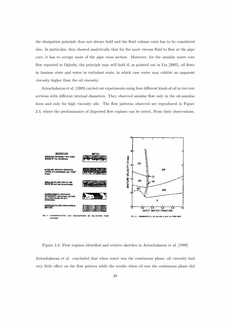
Arirachakaran et al. [1989] carried out experiments using four different kinds of oil in two test
sections with different internal diameters. They observed annular flow only in the oil-annulus
form and only for high viscosity oils. The flow patterns observed are reproduced in Figure
2.4, where the predominance of dispersed flow regimes can be noted. From their observations,
Figure 2.4: Flow regimes identified and relative sketches in Arirachakaran et al. [1989]
Arirachakaran et al. concluded that when water was the continuous phase, oil viscosity had
very little effect on the flow pattern while the results when oil was the continuous phase did
39

not allow the authors to reach any conclusion. As for the absence of water-annulus annular
flow type in all the examined cases, the authors proposed that the physical properties of the
oils used (density and viscosity) were not suitable to sustain a stable oil core.
Valle and Kvandal [1995] performed a study of the stratified oil/water flow pattern reporting
the dispersed phase distribution across the pipe section. They observed the dispersion of both
oil into water and water into oil; in particular, high dispersed fractions at the bottom or at
the top of the pipe where obtained when the difference in the phase superficial velocities was
greater than 0.6-0.7 m/s. The entrained fractions of oil into water and water into oil for constant
mixture velocities plotted against the input water fraction showed a marked U shape with the
lowest region around 0.4-0.6, suggesting some sort of equilibrium between the phases in that
region. An interesting remark is made by the authors regarding the fact that a water film on
the pipe wall was observed for all the flow pattern reported.
Annular flow was not observed by Angeli and Hewitt [1998] who studied co-current flow of
oil and water in horizontal pipes (test sections of stainless steel and acrylic resin were used in
different experiments). Angeli [1996] had used the same oil as in Angeli and Hewitt [1998] to
investigate the droplet distribution in oil-water flow in horizontal pipes. Measurements were
taken varying both the mixture velocity and the input water fraction for both test sections.
Again, annular flow was not observed while the encountered flow patterns were stratified and
stratified mixed flow, three-layer flow and dispersed flow depending on the input water fraction
and mixture velocity. Both steel and acrylic test sections were used in her study. The steel
section produced flow patterns more disturbed than those in the acrylic section for the same
inlet conditions; Angeli suggested that the difference could be attributed to a higher turbulence
in the steel section due to the material roughness. The different wettability of the two materials
was identified as a possible factor responsible for the wider velocity range over which oil is the
continuous phase in the acrylic pipe. Figure 2.5 reproduces the flow maps of Angeli [1996] for
the two test sections used in her experiment.
Trallero [1995] reported that for low oil and water superficial velocities the flow was gravity
dominated and the phases were segregated. He noticed in particular that for moderate water
fractions the oil-water interface was smooth and waveless while a further increase in the flow
rates caused the appearance of interfacial waves. Along the waves, water droplets in the oil
40

(a) (b)
Figure 2.5: Experimental flow maps for stainless steel pipe (a) and ’transpalite’ test section (b)(from Angeli [1996])
layer and oil droplets in the water layer can appear but both kind of droplets remained close
to the interface. Trallero then considered that outside of the stratified region different kinds
of dispersion could be encountered. For large water superficial velocities the flow was water
dominated and water vortices appearing at the interface entered the oil layer and tended to
displace it. On the other hand, oil was the dominant phase for small input water fractions.
Accordingly, Trallero reclassified the flow patterns for a number of investigations as in Tab 2.1.
Tab 2.2 (from Valle [2000]) proposes a possible reclassification to match the flow patterns in
Segregated flow Stratified flowStratified flow with mixing atinterface (ST&MI)
Dispersed flow (waterdominated)
Dispersion of oil in water andwater (Do/w&w)Oil in water dispersions (o/w)
Dispersed flow (oildominated)
Dispersions of waterin oil and oil in water(Dw/o&Do/w)Water in oil dispersions (o/w)
Table 2.1: Flow pattern classification according to Trallero [1995]
Angeli [1996] and Trallero [1995].
Nadler and Mewes [1997] studied the effects of emulsification and phase inversion on pressure
drop for different flow regimes of oil-water mixtures. They distinguished between dispersions
and emulsions, defining dispersions as those flow patterns with an oil and water layers flowing
41

Angeli [1996] Trallero [1995]
Stratified wavy (SW) Stratified flow with mixing atinterface (ST&MI)
Stratified wavy/drops (SWD) (ST & MI)Stratified mixed with an oillayer (SM/oil)
Dispersed water in oil and anoil region free of drops (w/o)
Stratified mixed with a waterlayer (SM/water)
Dispersed oil in water anda water region free of drops(o/w)
Three layer flow pattern (3L) Dispersed oil in water andwater in oil (Dw/o&Do/w)
Mixed (M) Water in oil dispersion (w/o)Oil in water dispersions (o/w)
Table 2.2: Relation between the flow pattern classification of Angeli [1996] and Trallero [1995]proposed by Valle [2000]
on top of each other, with the presence of a dispersed phase in one or both of the two layers.
Emulsions, instead, were defined as the flow pattern with one phase (continuous phase) occu-
pying the whole pipe cross section and the other phase (dispersed phase) uniformly distributed
within the continuous phase. In the authors’ experimental work, phase inversion was reported
to occur only in the form of layers of oil-in-water and water-in-oil flowing over a water layer
(region IIIb in Figure 2.6 (a)); phase inversion, therefore, involved only part of the pipe cross
section.
Lovick and Angeli [2004] considered the dual continuous flow pattern, where both phases
retain their continuity at the top and bottom of the pipe while there is inter-dispersion. In
their experiments, by increasing the mixture velocity the flow pattern changed from stratified
to dual continuous to dispersed flow. In the dual continuous flow pattern, pressure losses where
less than the corresponding values for pure oil flowing in the pipe.
2.2.1 Factors influencing oil/water flow pattern
Pipe inclination
When the pipeline is inclined, the gravity force acting on the fluids can be split into a
component parallel to the pipe axis and another component normal to it. While the latter
acts towards a stable configuration of the fluids, in the case of the former it is necessary to
distinguish between the situation where force opposes the fluid motion (case of pipe inclined
42

(a) (b)
Figure 2.6: Experimental flow maps presented in Nadler and Mewes [1997])
upwards) and the situation when the force enhances the fluid motion (case of pipe inclined
downwards).
Trallero [1995] reported the results of Scott [1985] on the flow pattern in inclined pipes.
In particular, at low oil and water superficial velocities the flow was stratified and exhibited
large amplitude rolling waves. The axial gravity component induced a local back flow in the
water phase at the bottom of the pipe (Rw-cou in Figure 2.7). Trallero further reported that
an increase in the water flow rate also increased the water momentum and the flow became
fully co-current (Rw-coc in Figure 2.7); however, large rolling waves were still observed. A
further increase in the flow rates enhanced the mixing of the liquids, dispersing the oil into the
water. For the highest superficial velocities, oil was emulsified in water. Trallero reclassified
the flow pattern identified by Scott, as in Figure 2.7. Trallero also reclassified the flow pattern
identified by Cox [1985] (Figure 2.8) who studied downward inclined pipes. He observed that
the interface was unstable at low oil-water flow rate ratios while the mixing of the phases
was reduced by increasing the oil superficial velocity. Further increasing the flow rate, Trallero
reported dispersion of the oil (Do/w & w) and at the highest velocities the oil became emulsified
43

Figure 2.7: Experimental flow pattern map, 15upward, Scott [1985] (from Trallero [1995])
Figure 2.8: Experimental flow pattern map, -15downward, Cox [1985] (from Trallero [1995])
44

in the water. The transition to dispersed flow was less affected by the pipe inclination than in
the case of upward inclined pipes.
An analysis of the flow patterns observed in three-phase oil/water/gas flow in horizontal
pipes was presented by Acikgoz et al. [1992]. The authors classified the observed flow patterns
into two main categories: oil-based and water-based flow patterns, on the basis of the extent of
the phase-wall contact surface. With appropriate combinations of total liquid mixture velocity
(with constant oil superficial velocity) and gas superficial velocity, different flow patterns were
obtained within the two main categories, namely plug flow, slug flow, stratified-wavy flow (either
dispersed or separated) and annular flow.
Pan [1996] proposed a flow pattern classification similar to the one by Acikgoz et al. [1992]
(diagram in Figure 2.9) based on the stratification or full dispersion of the liquid phases, the
continuous phase in case of dispersion within the liquid body and the flow pattern when the
gas and the total liquid mass are considered, as in two-phase gas-liquid flow.
Figure 2.9: Three-phase flow regime classification by Pan [1996]
Pan’s experiments underlined the importance of high gas superficial velocities to enhance the
mixing of the liquid phases. Interesting observations were reported on phase inversion involving
the oil and water phases: it was noted that phase inversion occurred suddenly and sharply and
when the experimental rig was set in the region of transition between water continuous and oil
continuous, unstable flows were observed inside the test section. Moreover, the higher pressure
losses were measured outside this unstable region, meaning that the higher pressure gradients
were not associated with phase inversion.
More recently, Oddie et al. [2003] conducted steady state and transient experiments of
water-gas, oil-water and oil-water-gas flow in a transparent, inclinable pipe using kerosene,
45

water and nitrogen. The pipe inclination was varied from 0(vertical) to 92and the flow rate
of each of the phases was varied over a wide range. They reported extensive results for hold-up
as a function of flow rates, flow pattern and pipe inclination. Segregated, semi-segregated,
semi-mixed, mixed, dispersed, and homogeneous flow patterns were observed. Close to the
Figure 2.10: (a) Observed water-gas flow patterns in inclined pipe; (b) Observed oil-water-gasflow patterns in inclined pipe (Oddie et al. [2003])
vertical position (between 0and 45) water and oil flow was dispersed and the two fluids mixed
easily. Approaching the horizontal position, stratified flow patterns appeared (segregated and
semi-segregated flow pattern). However, mixed, dispersed and homogeneous flows were still
observed. For downward inclinations, stratified flow prevailed and high flow rates were required
to disperse the phases.
Pipe diameter
Valle [2000] compared the experimental results by Stapelberg and Mewes [1990] and Nadler
and Mewes [1995a,b] concluding that the stratified flow region decreases as the tube diameter
46

increases and the region for fully dispersed flow (oil and water continuous dispersion) increases
for increasing tube diameter.
Mandal et al. [2007] studied oil and water flow in two pipes with different diameters, namely
0.025 m and 0.012 m, highlighting the differences in the observed flow patterns for the two test
section studied. In particular they reported the occurrence of the rivulet flow and the churn
flow pattern in the narrower pipe while the three-layer pattern appeared in the 0.025 m pipe
but not in the smaller tube. The authors attributed these differences to the increased effect of
surface tension and equilibrium contact angle in the narrow pipe.
Pipe material
The dependence of the flow pattern on the pipe material is of importance both in industrial
application and in the research field. Information on flow pattern, in fact, are often obtained by
easy and direct observation of transparent test sections while other more complex methods are
necessary for flows through metal pipes. The influence of the wettability on the flow properties
indicates that the results and the conclusions reached for transparent test sections cannot be
automatically extended to pipe made of other materials (Angeli and Hewitt [2000b]).
An example of different behaviour in pipes of different materials is provided in the work
of Angeli [1996]. The experimental data for steel test sections and acrylic ones showed more
homogeneous dispersion when using steel pipes; moreover, dispersion in the steel pipe could be
found at lower mixture velocities than in the acrylic section (1.3 m/s for the steel section and
1.7 m/s for the acrylic section.).
Angeli and Hewitt [2000b] made measurements for mixture velocities varying from 0.2 to
3.9 m/s and input water volume fraction from 6% to 86%. They observed that in general, the
mixed flow pattern appeared in the steel pipe at lower mixture velocities than in the acrylic
pipe, where, in addition, oil was the continuous phase for a wider range of conditions. Table
2.3 provides a summary of their finding.
Fluid viscosity
Urdahl et al. [1997] discussed the influence of emulsion viscosity on multiphase flow calcula-
tions; they stated that the viscosity of an emulsion usually depends on the following factors: (a)
the viscosity of the continuous phase; (b) the viscosity of the dispersed phase; (c) the amount
of dispersed phase; (d) shear rate; (e) average droplet diameter and drop size distribution; (f)
47

Flow pattern Remarks
Stratified wavy
This flow pattern existed over a higher range ofconditions in the acrylic pipe (mixture velocitiesup to 0.6 m/s) than in the steel pipe (mixturevelocities up to 0.3 m/s)
Three layers
This regime appeared at lower mixture velocitiesin the steel pipe (mixture velocities 0.7-1.03 m/sand water volume fractions 0.3-0.5) than in theacrylic one (mixture velocities 0.9 - 1.7 m/s andwater volume fractions 0.2-0.5)
Stratified mixed
For high water fractions a layer of oil dropswas observed on the top (SM/water), while forlow input water fraction a layer of water dropswas found on the bottom (SM/oil). While theSM/water regime prevailed over a wide range ofconditions in steel than in the acrylic pipe, theopposite happened for SM/oil regime
Fully dispersed or mixedThis flow pattern appeared at mixture velocitieshigher than 1.3 m/s in the steel tube and 1.7 m/sin the acrylic tube
Table 2.3: Influence of pipe material on flow patterns identified by Angeli and Hewitt [2000b]
emulsion stability; (g) temperature.
Arirachakaran et al. [1989] concluded that when water was the continuous phase, the effect
of oil viscosity on the flow pattern was limited. This seems to be confirmed by the data collected
by Oglesby [1979], as pointed out in Valle [2000].
Mixture velocity and input water fraction
Mixture velocity and input water fraction strongly influence the flow pattern in two-phase
liquid-liquid flow (Figures 2.2, 2.4, 2.5, 2.7, 2.8, 2.11). In general, the effects of mixture velocity
and input water fraction are coupled. Increasing the mixture velocity enhances turbulent effects
and the formation of emulsion, causing the transition from stratified to partially dispersed to
dispersed flow, which can be oil dispersed in water or vice versa depending on the properties of
the fluids and of the flow, including the input water fraction.
Beretta et al. [1997] focused their attention on small diameter pipes (approx. 3 mm in
diameter) where laminar flow is more common than in bigger pipes. Establishing laminar
annular flow with water wetting the pipe wall results in large reductions in pressure losses. By
increasing the mixture velocity, they observed different flow patterns, which they classified as
48

dispersed, intermittent (slug, bubbly and plug flow) and annular.
Arirachakaran et al. [1989], Angeli [1996] and Soleimani [1999] showed that the two key
variables affecting the flow pattern in oil-water mixtures are the mixture velocity and the input
water fraction. High mixture velocities promote the dispersion of the two phases with water-
in-oil regime at low input water fractions and oil-in-water regime at high input water fractions.
An increase in the mixture velocity produces a more homogeneous distribution of the dis-
persed phase (Angeli [1996], Angeli and Hewitt [2000b], Lovick and Angeli [2001]); Angeli and
Hewitt [2000b] also noted that for the same mixture velocity more homogeneous distributions
were obtained for small oil fractions.
Lovick and Angeli [2001] also reported how the slip ratio between the phases changed as a
consequence of changes in the oil input fraction. They observed that at high mixture velocities
the dispersed phase tended to move away from the pipe wall and towards the core of the flow.
For lower mixture velocities, however, turbulence could not disperse the phases homogeneously,
leading to stratification; the portion of the pipe wall wetted by the lesser phase may not be
negligible in this case.
Lovick [2004] observed dual continuous flow for mixture velocities up to 1.5 m/s for input
oil fractions ranging from 10% to 90%. For higher mixture velocities the dual continuous flow
pattern was limited to intermediate oil fractions. Moreover, vertical gradient in the dispersed
phase were detected; in particular, the lower the mixture velocity, the closer to the interface
the dispersed drops remain.
The experimental data and the flow map provided by Hussain [2004] seem to confirm the
importance of the slip ratio between the two phases, as was found by Lovick [2004]. The fluids
used in her experiments were tap water and Exxsol D80, a clear kerosene-like oil. Figure 2.11
shows an example of the flow pattern obtained by Hussain; she summarized the observed flow
patterns as follows: Stratified wavy [SW], Stratified wavy/drops [SWD], Stratified mixed/oil
layer [SM/O layer], Three-layer [3L], Stratified mixed/water layer [SM/W layer] and Dispersed-
flow [DF]. A first conclusion that can be drawn observing Figure 2.11 is that the effects of
the mixture velocity and input water fraction are strongly coupled for low mixture velocity.
For sufficiently high mixture velocities, instead, the flow pattern observed is dispersed flow,
independently from the water cut. It can be observed that for low mixture velocities and low or
49
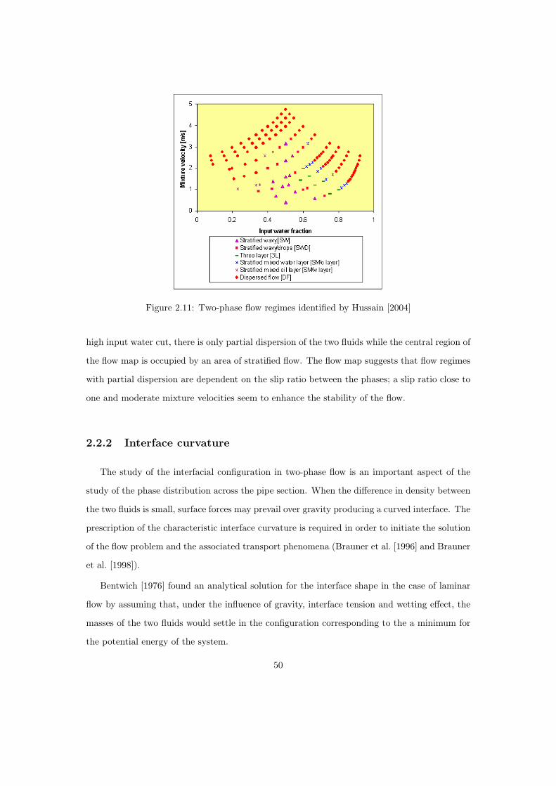
Figure 2.11: Two-phase flow regimes identified by Hussain [2004]
high input water cut, there is only partial dispersion of the two fluids while the central region of
the flow map is occupied by an area of stratified flow. The flow map suggests that flow regimes
with partial dispersion are dependent on the slip ratio between the phases; a slip ratio close to
one and moderate mixture velocities seem to enhance the stability of the flow.
2.2.2 Interface curvature
The study of the interfacial configuration in two-phase flow is an important aspect of the
study of the phase distribution across the pipe section. When the difference in density between
the two fluids is small, surface forces may prevail over gravity producing a curved interface. The
prescription of the characteristic interface curvature is required in order to initiate the solution
of the flow problem and the associated transport phenomena (Brauner et al. [1996] and Brauner
et al. [1998]).
Bentwich [1976] found an analytical solution for the interface shape in the case of laminar
flow by assuming that, under the influence of gravity, interface tension and wetting effect, the
masses of the two fluids would settle in the configuration corresponding to the a minimum for
the potential energy of the system.
50

Brauner et al. [1996] employed a minimal energy consideration to predict the interface
location and shape assuming a constant curvature (circular arc). The authors calculated the
total energy variation for unit length of a horizontal pipe as
∆E
L=
∆(Ep + Es)L
= R3ρ2g
(1− ρ1
ρ2
)[sin3 φ0
sin2 φ∗(ctg φ∗ − ctg φ0) (π − φ∗ + sin (2φ∗) /2)
+23
sin3 φp0
]+ Eo
[sin φ0
π − φ∗
sinφ∗− sin φp
0 + cos θ (φp0 − φ0)
], (2.1)
where Ep and Es are the potential and surface energy of the system, Eo =2σ12
(ρ2 − ρ1) gR2
is the Eotvos number and the geometric parameters in Equation (2.1) can be obtained from
Figure 2.12 The value of the curvature from Equation (2.1) depends on the Eotvos number, the
Figure 2.12: Two phase flow configuration with curved interface (from Brauner et al. [1996])
wettability angle of the two phases θ and, indirectly, from the hold up ratio A1/A2; monograms
may be built, which show the variation of the curvature as a function of one of the variables,
keeping the other two as parameters, as in those reproduced in Figure 2.13. As pointed out
by the authors, for gravity dominated systems, Eo → 0 and Equation (2.1) returns a flat
interface. On the other hand, in systems dominated by surface effects (Eo → ∞), the steady
interface curvature is dominated by the wettability angle and φ0. Brauner et al. [1998] applied
Equation (2.1) together with the momentum equations for the two phases within the framework
of the two-fluid model and studied the curvature of the interface for laminar-laminar flow and
turbulent-turbulent flow.
Soleimani [1999] obtained an exact formulation for the interface coordinates in equilibrium
conditions imposing that the pressure jump across the interface has to be balanced by effective
pressure due to surface tension. The solution, consequently, was obtained from integration of
51

(a) (b)
Figure 2.13: Interface curvature (from Brauner et al. [1996])
52

the Young-Laplace equation.
Like in Soleimani, a force balance across the interface is applied in Gorelik and Brauner [1999]
to find an exact solution for the interface coordinates. Curvature was not assumed constant,
although symmetry was assumed with respect to the vertical diameter of the pipe section. The
authors also found an approximate solution for the interfacial curvature by assuming constant
curvature and solving the variational problem of minimising the total free energy per unit tube
length, as done in Brauner et al. [1996]. An exact analytical solution was obtained in the case
of unidirectional axial laminar flow. Figure 2.14 shows an example of comparison between the
solution obtained with the constant curvature approximation (Brauner et al. [1996]) and the
exact solution, as calculated by Gorelik and Brauner [1999]. The solution obtained assuming
Figure 2.14: Comparison between approximated constant curvature interface (dashed lines,Brauner et al. [1996]) and exact solution (solid lines, Gorelik and Brauner [1999]) for wettabilityangle = 15 (from Gorelik and Brauner [1999])
constant curvature closely approximates the exact solution; the authors noticed that deviation
become larger for θ → 0 while the comparison improves as θ → π/2. As observed by the
authors, the assumption of constant curvature is legitimate when gravity effects can be ignored,
such as for microgravity conditions and for fluids of comparable densities.
Ng et al. [2001] used the solution of the Young-Laplace equation to calculate the interface
53

shapes for various Bond numbers, contact angles and holdup. According to their results, when
the dominant parameter is the surface tension (small Bond numbers) the interface is strongly
curved while when there is a large difference in the fluid densities (large Bond numbers) the
effects of the surface tension are weaker and the interface is almost flat, curving only close to
the pipe walls.
2.3 Pressure gradient and mixture viscosity
Charles and Redberger [1962] computed the liquid flow rate for five hypothetical oils ranging
in viscosity from 4 to 1500 mPa s in the presence of water, by computing the oil and velocity
profiles for a series of arbitrary oil-water interface positions. In general, according to their
(a)(b)
Figure 2.15: Pressure gradient reduction factors as a function of interface position and percent-age of water in the flowing stream (from Charles and Redberger [1962])
calculation, the greater the oil viscosity, the greater is the rate of increase of the pressure
gradient reduction factor with increasing water percentage, although for the higher oil viscosities
the curves are very close together (Figure 2.15). For the theoretical fluids considered, the
percentage of water needed to bring about the maximum benefit varied from 12% for a 4.0 cP
oil to 93% for a 1500.0 cP oil. For all viscosities the pressure gradient reduction factor decreases
very rapidly as the water percentage approaches 100.
The results of Charles and Redberger [1962] confirmed what was obtained previously by
Charles et al. [1961]. The latter investigated the horizontal flow of equal density oil-water
54

mixture in a 1-inch diameter horizontal pipeline using oil viscosities 6.29, 16.8, 65.0 cP and
superficial velocities ranging from 0.03 to 1.06 m/s with input oil-water ratios ranging from
0.1 to 10.0. The measurements indicated that for given oil flow rate the pressure gradient was
reduced to a minimum by the addition of water, provided the oil was not in turbulent state.
Maximum pressure gradient reduction factors varied from 1.7 for the 6.29 mPa s viscosity oil
to 10 for the 65.0 mPa s viscosity oil at input oil-water ratios of 4.5 and 1.0 respectively.
An example of the curves of pressure gradients obtained by Charles and Redberger is shown in
Figure 2.16. It is apparent that, for oil flow rate below 0.3 m/s, a reduction in pressure gradient
Figure 2.16: Pressure gradients for the oil of viscosity 6.29 cP as a function of the input oil-waterratio and oil velocity. (Charles et al. [1961])
was obtained by the addition of water. The factors by which the pressure gradients were reduced
were largest at the lowest oil flow rates. For oil velocities above 0.3 m/s a pressure gradient
reduction was not observed and an increase in pressure gradient was detected immediately
upon the addition of water. However, this consideration cannot strictly be extended to the
other oils examined in that work since their behaviour showed significant dissimilarities. It
may nevertheless be concluded from the results that the addition of increasing amount of water
to oil, which is originally in laminar flow, lowers the pressure gradients to a minimum, after
55

which the addition of more water increases the pressure gradient and, with sufficient water, the
pressure gradient exceeds the pressure gradient for oil flowing alone.
Soot and Knudsen [1973] derived empirical and theoretical equations for predicting pressure
losses for two phase liquid-liquid flow in pipes. The authors investigated the effect of the
dispersed drop size on pressure losses. The drop size distribution of the dispersed phase was
determined from flow photographs. Drop size seemed to have a small effect on pressure losses
but this effect appeared to be swamped by errors affecting both the measurements and the
calculations. From their observations it is possible to conclude that the pressure drop decreases
for increasing drop size with a sensitivity to high concentrations.
Ward and Knudsen [1967] performed a study of friction losses, velocity profiles and drop
size distributions of liquid-liquid dispersions in turbulent flow. An interesting problem brought
to attention by Ward and Knudsen is whether and when it is possible to apply methodologies
developed for single phase flow to two-phase flow for the prediction of momentum and heat
transfer. The required condition is that the mixture should behave as a homogeneous fluid.
The authors referred to the work of Baron et al. [1953], who had concluded that, when the
particle diameter is small compared to the size of the region of viscous flow, a single-phase
equation can be used to describe the two-phase flow. Baron et al. [1953] correlated the particle
diameter to the Kolmogorov microscale and, by considering the ratio of the inertia forces and
the drag forces acting on the dispersed phase, derived the following criterion that determines
when a dispersion behaves as a single phase homogeneous fluid:
Rec
(dp
D
)2 (ρd
ρc
)≤ 1, (2.2)
where Rec is the Reynolds number based on viscosity of continuous phase, ρc and ρd are the
continuous and dispersed phase densities respectively and D is the pipe diameter. According
to Ward and Knudsen, applications of equation (2.2) to a liquid-liquid dispersion flowing in a
4-in pipe at Rec = 10000 indicates that the drop diameter should be less than 1 mm. Ward and
Knudsen performed experimental studies with a commercial petroleum solvent and two clear,
highly refined oils with large differences in viscosity. Examining the results of their experiments
56

they modified Equation (2.2) in the form:
Re
(d32
D
)2 (ρd
ρe
)≤ 2, (2.3)
where Re is the Reynolds number based on the effective viscosity of the dispersion and ρe is the
density of dispersion and d32 is the dispersed phase droplets mean Sauter diameter. Equation
(2.3) provides a tool for determining whether oil-in-water dispersions behave as homogeneous
Newtonian fluids. Although the criterion is of the same order of magnitude of that derived by
Baron et al., Ward and Knudsen are quick to point out that their conclusion is strictly limited
to the three oil-in-water systems they investigated.
An approach similar to the one of Baron et al. [1953] was adopted by Cengel et al. [1962],
who assumed that the dispersion behaved as a single-phase fluid and used measured friction
factors to calculate an effective viscosity of the mixture. Cengel et al. were aware of the
limitations imposed by Baron et al. to the particle size and, although no direct measurement
of the droplets size is performed, indirect calculations showed the dispersed droplets to be of
order of 10-25 µm, matching the indication in Baron et al. [1953]. Moreover, Cengel et al. [1962]
assumed that the dispersed phase was uniformly dispersed throughout the continuous phase and
no slip between the dispersed and continuous phase, i.e. constant concentration throughout the
system. The measured pressure losses were used to calculate the effective viscosity both for
laminar flow and turbulent flow by means of the relationship derived by Langhaar (laminar flow)
and a Blasius-like correlation for the liquid-wall friction factor in turbulent flow. The viscosities
calculated from vertical flow data were found to be considerably lower than the corresponding
laminar viscosities, and the difference increased with an increase in the dispersed phase (oil)
concentration. The low values of viscosity obtained from turbulent data indicated that the
pressure drop in turbulent flow of emulsions (for a given flow rate) was less than the value
expected for laminar flow; in other words, the emulsions exhibited drag reduction behaviour in
turbulent flow.
Faruqui and Knudsen [1962] studied the momentum and heat-transfer characteristics of an
unstable liquid-liquid dispersion made up of a kerosene-like petroleum solvent and water and
containing up to 50% dispersed phase. Velocity and temperature profiles, friction factors and
57

heat transfer coefficient were obtained for dispersions of various concentrations in turbulent
flow in a vertical tube. The velocity profiles were used to calculate the effective viscosities of
the emulsions by means of a logarithmic law in the form:
u+ = CA + CB log(y+µm
), (2.4)
where u+ is the dimensionless velocity, y+ is the dimensionless distance from the pipe wall,
µm is the mixture viscosity and CA and CB are functions of the dispersion concentration. The
analysis of the velocity profile suggested that the dispersions manifested Newtonian behaviour
at low mixture velocity and non-Newtonian characteristics at high mixture velocity.
Charles and Lilleleth [1966] adopted the parameters X and Φ introduced by Lockhart and
Martinelli [1949] to correlate pressure loss data for the stratified flow of two immiscible liquids
in the laminar-turbulent regime. The parameters were defined in the form:
X2 =
(dpdz
)o(
dpdz
)w
Φ2 =
(dpdz
)TP(
dpdz
)o
(2.5)
where(
dpdz
)o
and(
dpdz
)w
are the pressure gradients for the oil and water flowing alone in the
channel respectively and(
dpdz
)TP
is the two phase (oil-water mixture) pressure gradient. It is
worth remembering that the work of Lockhart and Martinelli [1949] focused on the pressure
gradient of gas-liquid mixtures in horizontal pipes. Charles and Lilleleth [1966] examined the
flow in one rectangular and two circular cross section pipes. Data from three set of experiments
with liquid-liquid were fitted reasonably well using Equation (2.5), with a maximum deviation
of approximately 24%.
Theissing [1980], as reported by Angeli [1996], Angeli and Hewitt [1998] and Valle [2000],
proposed an expression for the pressure gradients that is supposed to be independent of the
particular flow regime:
(dp
dz
)
TP
=
[(dp
dz
) 1neT
otM
(Mo
Mt
) 1eT
+(
dp
dz
) 1neT
wtM
(Mw
Mt
) 1eT
]neT
, (2.6)
where:
58

eT = 3− 2
2√
ρo
ρw
1 +ρo
ρw
0.7n
n =n1 + n2
(1χ
)0.2
1 +(
1χ
)0.2
n1 =
ln
(dp
dz
)
oM(dp
dz
)
otM
ln
(MoM
Mt
) n2 =
ln
(dp
dz
)
wM(dp
dz
)
wtM
ln
(MwM
Mt
) .
(2.7)
In Equation (2.7) ρo and ρw are the oil and water density, Mo and Mw are the oil and water mass
flow rates,(
dpdz
)oM
and(
dpdz
)wM
are the pressure gradients when oil and water flow alone at
Mo and Mw respectively,(
dpdz
)otM
and(
dpdz
)wtM
are the pressure gradients when oil and water
flow alone at the total mixture mass flow rate. While the model in Lockhart and Martinelli
[1949] was specifically developed for gas-liquid flow, Theissing model could be applied both to
gas-liquid and liquid-liquid flow.
Stapelberg and Mewes [1994] studied the slug flow of oil, water and gas in horizontal pipes
and observed that, for lower gas flow rates, the pressure losses associated with oil flowing on
top of water had an intermediate value between the pressure losses measured for the two-phase
oil-gas flow and the two-phase water-gas flow. For higher gas flow rate, the three-phase pressure
losses were smaller than the corresponding two-phase gas-water flow. Moreover, the authors
reported that the oil fraction had little effect on the pressure losses when the mixture velocity
was kept constant. For liquid-liquid flow they followed the suggestion of Charles and Lilleleth
[1966] by presenting their data in a Lockhart-Martineli diagram, calculating the parameter of
the model in a form that accounts for the flow pattern.
Arirachakaran et al. [1989] adopted the pressure gradient prediction model for stratified flow
developed by Malinowsky [1975]. The model assumes that the flow is stratified, with a smooth
interface and with neither relative motion nor mass transfer between the phases. Furthermore,
the total wall shear stress is calculated as the sum of the water and oil wall shear stress, which
in turn are calculated as a fraction of the wall shear stress which would be encountered if each
59

phase was flowing alone in the pipe at the same velocity. As a weighting factor, they used
the fraction of the pipe occupied by each phase expressed through the oil and water wetted
perimeter So and Sw:
τW = τWo + τWw =So
2πRτ ′Wo +
Sw
2πRτ ′Ww. (2.8)
With simple steps, the following expression is derived:
(dp
dz
)
TP
=So
2πR
(dp
dz
)
o
+Sw
2πR
(dp
dz
)
w
, (2.9)
which correlates the two-phase pressure gradient(
dpdz
)TP
to the pressure gradients that would
occur if either phase was flowing alone in the pipe at the same velocity ((
dpdz
)o
and(
dpdz
)w
for
oil and water respectively).
Pal [1993] presented results concerning the laminar and turbulent flow behaviour of unstable
(without any added surfactant) and surfactant-stabilised water-in-oil emulsions. Both emulsions
without surfactants exhibited drag reduction behaviour in the turbulent regime. Drag reduction
seemed to be connected with the amount of dispersed phase fraction; however, the effect was
more severe in water-in-oil emulsions. Conversely, emulsions with added surfactants showed
little drag reduction and in some case the drag reduction phenomenon disappeared completely.
Therefore, Pal indicated that single-phase equations should be applied to emulsions with added
surfactants. Pal related the drag reduction behaviour to the break-up and coalescence of dis-
persed phase drops. The presence of surfactants inhibits these processes and, according to Pal,
this is the reason for the absence of drag reduction when surfactants are added to the mixture.
Results similar to those of Pal [1993] are reported also by Angeli and Hewitt [1998], who plotted
friction factors against mixture velocity for a steel pipe and found that the friction factors for
water-in-oil emulsions are much lower than those for pure oil flow but the friction factors for
oil-in-water flow do not differ much from single-phase data.
An expression for the calculation of the viscosity of suspensions of solid particles for infinite
dilution was proposed by Einstein [1906] in the form:
µM
µc= 1 + 2.5φ, (2.10)
60

where µM is the viscosity of the suspension, µc is the viscosity of the continuous phase and φ
is the volumetric concentration of the dispersed phase.
Equation (2.10) was developed for solid sphere immersed in a fluid. Taylor [1932] proposed
an expression similar to the one proposed by Einstein, which can be applied when the dispersed
phase is made up of spherical fluid particles as:
µM
µc= 1 + 2.5φ
(0.4 + µd
µc
1 + µd
µc
). (2.11)
As in the case of Einstein’s expression, the expression by Taylor is supposed to work for any
dilute dispersion.
Guth and Simha [1936] modified the expression proposed by Einstein to account for the
interaction between particles and to increase the range of dispersed phase fraction over which
the formula could be applied:µM
µc= 1 + 2.5φ + 14.1φ2. (2.12)
Eilers [1941, 1943] formulated the following expression:
µM
µc=
(1 +
2.5φ
2 (1− Caφ)
)2
, (2.13)
where Ca is a coefficient tuned by the author to fit experimental data. The values reported for
Ca range from 1.28 to 1.35
An improvement to Taylor’s expression was provided by Oldroyd [1953] who considered
the case of droplets with partial internal circulation. Leviton and Leighton [1936], Richard-
son [1950], Mooney [1951] and Barnea and Mizrahi [1973] proposed exponential relationships
between the relative viscosity of the emulsion and the dispersed phase concentration.
Mooney [1951] attempted to extend and apply Einstein’s expression to a suspension of finite
concentration and theoretically derived:
µM
µc= exp
(2.5φ
1− Ckφ
), (2.14)
where Ck is the self-crowding factor. With rudimentary arguments Mooney derived the upper
61

and lower limits for the allowed values of Ck, proposing 1.35 < Ck < 1.91. Equation (2.14)
is valid for monodisperse systems; for polydisperse systems the author introduced a variable
factor, λij , which accounts for the crowding of spheres of radius rj by spheres of radius ri.
A similar expression was proposed by Barnea and Mizrahi [1973]:
µM
µc= exp
(CK1φ
1− CK2φ
). (2.15)
From the data presented in Thomas [1965] Barnea and Mizrahi derived CK1 = 2.66± 0.20 and
CK2 = 1.00± 0.03
A simple extension of the work of Einstein was proposed by Brinkman [1952]:
µM =µc
(1− φ)2.5 . (2.16)
The author claimed that his expression could be applied to higher concentration if the result
for infinitesimal dispersions was known. In the derivation of his formula, he used Einstein
expression for the solution at infinitesimal concentration.
An identical expression was obtained in Roscoe [1953], who did not cite Brinkman’s work.
Roscoe, however, pointed out in the derivation process that the expression derived is strictly
valid in the limiting case of extreme diversity in the drop size distribution.
For the case of spheres of equal size, Roscoe made a distinction between high and low
concentration. For the first case, he referred to the results of Vand [1948] who pointed out
the importance of collisions between the dispersed spheres. Roscoe observed that a certain
amount of liquid is trapped between the spheres in actual contact and this increases the effective
concentration of the suspension. For very high concentrations spheres may form aggregates of
three or more, closely packed and roughly spherical in form, yielding an increase in the effective
concentration by a factor 3√
2/π (∼= 1.350). Equation (2.16) was modified accordingly to
account for this increase, taking the form:
µM =µc
(1− 1.35φ)2.5 . (2.17)
Figure 2.17 compares Equations (2.16) and (2.17) with data by Eilers [1941] and Ward and
62

Figure 2.17: Relative viscosity of suspensions of spheres - A, Einstein relation; B, curve forspheres of very diverse sizes; C curve for spheres of equal size. Diamonds = spheres of diversesizes (Eilers [1941]); Circles = spheres of 17:1 size ratio (Ward and Whitmore [1950]) - fromRoscoe [1953]
Whitmore [1950], the first set of data having a more remarkable diversity in disperse phase
drop size.
No explicit formula is given by Roscoe for low concentrations and spheres of equal size.
However, he shows approximately that, because of the interaction between droplets, the value
of the effective concentration increases rapidly to 1.35φ for increasing φ, allowing the application
of equation (2.17).
Pal and Rhodes [1989] compared the experimental results of van der Waarden [1954] with
the prediction of equations (2.16) and (2.17), as in Figure 2.18, which shows that both equations
largely overpredict the experimental data.
Pal and Rhodes [1985] developed an equation that correlated the relative viscosities of both
oil in water and water in oil emulsions as a function of normalised dispersed phase concentration,
in the form:
µM
µc=
[1 +
1.342φ/ (φ)µr=100
1.194− φ/ (φ)µr=100
]2.226
, (2.18)
63

Figure 2.18: Comparison of van der Waarden [1954] data with Equations (2.16) and (2.17)(from Pal and Rhodes [1989])
where (φ)µr=100 is the concentration of dispersed phase at which the relative viscosity of the
emulsion becomes 100 and will depend on all the possible factors which affect the viscosity of
emulsions. Pal and Rhodes recommended the use of Equation (2.18) for the concentration range
for which it was tested, i.e. φ/ (φ)µr=100 < 1. Equation (2.18) was reformulated in modified
form by Pal and Rhodes [1989], where the fit was extended to a larger set of data (van der
Waarden [1954], Eilers [1941, 1943] and 14 sets of data collected by the authors) as shown in
Figure 2.19. Equation (2.18) then becomes:
µφ
µc=
[1 +
φ/ (φ)µr=100
1.187− φ/ (φ)µr=100
]2.492
. (2.19)
In the same paper, Pal and Rhodes offer a theoretical approach that accounts for the effects
of hydration and flocculation of dispersed particles through a hydration factor CK0 and a
flocculation factor CKF . With assumptions similar to those in the derivations by Roscoe [1953]
and Brinkman [1952] they arrived to the following expression:
µM
µc= [1− CK0CKF (γ)]−2.5
. (2.20)
64
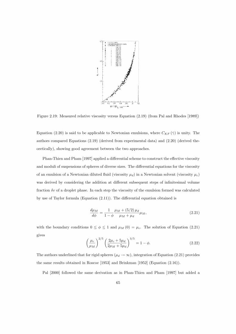
Figure 2.19: Measured relative viscosity versus Equation (2.19) (from Pal and Rhodes [1989])
Equation (2.20) is said to be applicable to Newtonian emulsions, where CKF (γ) is unity. The
authors compared Equations (2.19) (derived from experimental data) and (2.20) (derived the-
oretically), showing good agreement between the two approaches.
Phan-Thien and Pham [1997] applied a differential scheme to construct the effective viscosity
and moduli of suspensions of spheres of diverse sizes. The differential equations for the viscosity
of an emulsion of a Newtonian diluted fluid (viscosity µd) in a Newtonian solvent (viscosity µc)
was derived by considering the addition at different subsequent steps of infinitesimal volume
fraction δv of a droplet phase. In each step the viscosity of the emulsion formed was calculated
by use of Taylor formula (Equation (2.11)). The differential equation obtained is
dµM
dφ=
11− φ
µM + (5/2) µd
µM + µdµM , (2.21)
with the boundary conditions 0 ≤ φ ≤ 1 and µM (0) = µc. The solution of Equation (2.21)
gives (µc
µM
)2/5 (2µc + 5µd
2µM + 5µd
)3/5
= 1− φ. (2.22)
The authors underlined that for rigid spheres (µd →∞), integration of Equation (2.21) provides
the same results obtained in Roscoe [1953] and Brinkman [1952] (Equation (2.16)).
Pal [2000] followed the same derivation as in Phan-Thien and Pham [1997] but added a
65

factor that takes into account the presence of adsorbed surfactant on the drop surface.
Johnsen and Rønningsen [2003] compared experimental data for water-in-oil emulsions with
water cuts in the range 0-90% against a temperature-dependent Richardson-type correlation
(proposed in Rønningsen [1995]) and to Equations (2.14), (2.19) and the model proposed in Pal
[2000]. The expression proposed in Rønningsen [1995] is
ln(
µM
µc
)= C1 + C2T + C3φ + C4Tφ, (2.23)
where T is the temperature. From their comparisons, Johnsen and Rønningsen [2003] concluded
that the best results were given by Equation (2.19) provided that the equation was tuned to
measured data; Mooney’s equation was a valid alternative and for low and medium water cuts
the viscosity returned by Equation (2.23) was comparable to the values provided by Mooney,
although slightly lower.
Pal [2001] presented a comparison between the viscosity models of Choi and Schowalter
[1975], Yaron and Gal-Or [1972] and Phan-Thien and Pham [1997] The first two relations are
derived from a cell model approach and are expressed in the form:
µφ
µc= 1 + I
[φ1/3
]φ, (2.24)
where I is a known function whose expression is given in the respective papers. Pal [2001]
compared the correlations with 19 sets of data, reaching the conclusion that the model of Yaron
and Gal-Or [1972] gives the best prediction for the viscosity of concentrated emulsions over a
wide range of dispersed phase fraction and viscosity ratio. The other two models examined
gave good predictions at low dispersed phase fractions only. At high dispersed phase fractions
the model of Phan-Thien and Pham [1997] underpredicts the relative viscosity of the mixture
whereas that of Choi and Schowalter [1975] overpredicts it.
66

2.4 Drop size and drop size distribution
2.4.1 Drop size
The drop size of dispersed phase is often described by use of one of the following quantities:
d10 weighted average drop size,∫∞0
d′p (d′) dd′
d32 Sauter mean drop diameter,
∫∞0
d′3p (d′) dd′∫∞0
d′2p (d′) dd′
d50 drop diameter below which 50% of the volume is found
d95 drop diameter below which 95% of the volume is found
d99 drop diameter below which 99% of the volume is found
where p (d′) dd′ is the probability for a drop of having diameter in the interval d′ − d′ + dd′.
Ward and Knudsen [1967] carried out experiments exploring the range of dispersed phase from
a value close to 0% up to 50% and proposed that the mean Sauter diameter of the dispersed
drops depends on φ0.4, where φ is the dispersed phase concentration. Angeli [1996] agreed
with the results of Ward and Knudsen, but her study covered dispersions that ranged from 3%
to 10%; however, it should be noted that Ward and Knudsens data were very scattered and
also showed that when the dispersed phase concentration increased, the peak in the drop size
distribution shifted towards small diameters.
Many of the available studies on drop size in liquid-liquid dispersion are related to stirred
tanks and less work has been done on dispersions occurring in pipeline flow. In his fundamental
study, Hinze [1955] calculated the maximum stable drop diameter postulating that the forces
acting on a drop of diameter d undergoing deformation and breakup are the surface force τ
(whether viscous stress or dynamic pressure), the surface tension of order of magnitude σ/d
and viscous stresses of order of magnitude µd
d
√τρd
.
Hinze argued that in turbulent flow the forces determining the size of the largest drops
are the dynamic pressure forces, which are caused by changes in velocity over distances at the
most equal to the diameter of the drop. Assuming that the fluctuations of wavelength 2d are
the source of the dynamic pressure responsible for the breakage of the largest drops, Hinze
calculated:
dmax
(ρc
σ
) 35
ε25 = C, (2.25)
67

where C is a constant. Using data provided by Clay [1940], which were obtained for annu-
lar turbulent field between coaxial rotating cylinders, Hinze assumed that dmax ' d95 and
determined C = 0.725. It is worth noting that, apart from the hypothesis of isotropic and
homogeneous turbulence where Kolmogorov energy distribution is valid, Hinze further assumed
dilute dispersions under non-coalescing conditions.
For the breakup of drops in turbulent liquid flow, Levich [1962] used the force balance
applied by Kolmogorov [1949] (forces due to dynamic pressure difference at two sides of the
drop, counteracted by surface tension forces) for the calculation of the maximum stable diameter
that can resist the deformation produced by the action of small eddies:
dcrit
2= L
25d
(σ
CDρ
) 35√
2u
65
, (2.26)
where CD ∼ 0.5 is the drag coefficient for flow past a drop and Ld is a characteristic dimension
of the drop. Levich [1962] also considered the case when ρc ¿ ρd (e.g. breakup of drops in
turbulent gas flow), modifying Equation (2.26) so as to account for the density ratio of the two
phases:dcrit
2=
(σ
CDρc
) 35
(ρc
ρd
) 25 L
25d
u65
(2.27)
Interestingly, Levich also observed that close to the wall, velocity variations are sharper than
in the core flow and, as a consequence of the differences in the local dynamic pressure, the
maximum stable drop in the proximity of the wall will be smaller than in the core region.
Hughmark [1971] combined together the external force due to the dynamic pressure acting
on the drop and the sum of the surface force that opposes the drop deformation and the viscous
stresses of the drop, obtaining the balance:
1.69u2∗ρc =
σ
dmax+ 1.3
µd
dmaxu∗
√ρc
ρd, (2.28)
from which the maximum drop diameter can be derived.
68
Starting from Hinze’s work, Sleicher [1962] proposed different expressions for the non-
dimensional groups introduced by Hinze, deriving:
We
õdub
σ= 38
[1 + 0.7
(µdub
σ
)0.7]
, (2.29)
where We = dmaxρcu2b
σ and ub is the bulk velocity. While Hinze considered turbulence in the
core region of the pipe, Sleicher’s derivation employed the universal profile of velocity and is
therefore applicable close to pipe wall.
Sleicher’s experiments were conducted with a 1 12 diameter pipe. Paul and Sleicher [1965]
conducted experiments on a 12 pipe ( 1
3 of that used by Sleicher [1962]) and found for C in
Equation (2.29) the value 43 instead of 38, thus concluding that dmax is proportional to D−0.1.
From the work of Hinze [1955] and Levich [1962], Hesketh et al. [1987] derived an expression
for the maximum stable drop diameter accounting for the drop deformation in the calculation
of the capillary pressure term:
dmax =
[(Wecrit
2
)0.6](
σ0.6
(ρ2cρd)
0.2
)(ε)−0.4
. (2.30)
Equation (2.30) is further modified to include the stabilising effect of viscous forces on the drops
by adding a viscosity group NV i following Calabrese et al. [1986]:
dmax = Cn
[(Wecrit
2
)0.6](
σ0.6
(ρ2cρd)
0.2
)(ε)−0.4 (1 + CBNV i)
0.6, (2.31)
where CB = 1.5 (Berkman and Calabrese [1985])
Angeli and Hewitt [2000a] reported data on drop size and drop size distribution for dis-
persed volume fractions between 3.4% and 9% and continuous phase velocity ranging from 1.1
to 1.7 m/s. Data reported in the paper were collected using both steel and an acrylic test sec-
tions. A comparison is made between the experimental data and the model proposed by Hinze
[1955], Sleicher [1962], Kubie and Gardner [1977], Hesketh et al. [1987]. The best fits of the
experimental data were given by the Sleicher [1962] and Kubie and Gardner [1977] correlations,
although it is observed that they were not able to account for the effects of the pipe material.
69

The Hesketh et al. [1987] correlation gave results similar to Hinze [1955], which underpredicted
the experimental data in all cases.
More recently Brauner [2001] and Brauner and Ullmann [2002] have extended the work of
Kolmogorov and Hinze to dense dispersions. Brauner [2001] calculates the mean energy dissi-
pation rate in Equation (2.25) as a function of the liquid-wall friction factor and the continuous
phase velocity as:
ε =4τuc
Dρc (1− φd)=
2u3cf
D
ρm
ρc (1− φd), (2.32)
which, together with (2.25) provides:
(dmax)0 =(
dmax
D
)
0
= 0.55(
ρcu2cD
σ
)−0.6 [ρm
ρc (1− φd)
]−0.4
. (2.33)
Equation (2.33) gives the maximum stable drop diameter for dilute dispersions, with the rec-
ommendation:
1.82Re−0.7c <
dmax
D< 0.1. (2.34)
For dense dispersions, the coalescence process between drops cannot be neglected. Brauner
[2001] observed that the drop tendency to coalesce is contrasted by the turbulent energy carried
by the continuous phase. Therefore, she equated the surface energy production of the dispersed
phase to the rate of turbulent energy supply by the continuous phase, obtaining:
ρcu′2
2Qc = CH
6σ
dmaxQd, (2.35)
where Qc and Qd are the flow rates of the continuous and dispersed phase respectively and CH
is a constant of order 1. Remembering Equation (2.32) and assuming v2 = 2 (εdmax)2/3, one
obtains from Equation (2.35):
(dmax)ε =(
dmax
D
)
ε
= 2.22C3/5H
(ρcu
2cD
σ
)−0.6 [ρm
ρc (1− φd)
]−0.4 (φd
1− φd
)0.6
, (2.36)
70

and the conditions in (2.34) still hold. According to Brauner [2001], the maximum drop diameter
should be taken as:dmax
D= max
(dmax
D
)
0
,
(dmax
D
)
ε
. (2.37)
Equations (2.33), (2.36) and (2.37) are the basic equations of the model named in Brauner
[2001] as the H-model. Adopting a line of derivation similar the one used in the H-model,
Brauner also developed the K-model that utilises the suggestions of Hughmark [1971] and the
results of Kubie and Gardner [1977] as starting points, giving:
(dmax
D
)
0
= 30ρc
ρmWe−1
c Re0.2c (2.38)
(dmax
D
)
ε
= 174CKWe−1c Re0.2
c
ρc
ρm
(φd
1− φd
). (2.39)
2.4.2 Drop size distribution
Studies on drop size distribution were presented by Ward and Knudsen [1967] and Kubie
and Gardner [1977]. Collins and Knudsen [1970] reported that no distribution law with any
theoretical basis could be found which correlated experimental distributions.
Karabelas [1978] obtained water drop size spectra using two liquid hydrocarbons as contin-
uous phases. He reported that the measured spectra showed a remarkable similarity and could
be fitted by either a Rosin-Rammler type of equation (Figure 2.20 (a)),
V = exp[−
(d
d95
)n], (2.40)
or an upper limit log-normal probability function (Mugele and Evans [1951]) (Figure 2.20 (b)):
V =12
exp [1− erf (Cδz)] , (2.41)
where z = ln[
ζd
dmax − d
]and ζ and Cδ are parameters obtained from experimental data. The
71

(a) (b)
Figure 2.20: Drop size distribution of water in kerosene represented by a Rosin-Rammler typeof function (a) and an upper limit log-probability function (b) for U = 2.98 m/s and 2.22 m/s(from Karabelas [1978])
72

mean Sauter diameter d32, and d95 were derived for the log-normal distribution in the form:
d32 =dmax
1 + ζ exp[
14C2
δ
] , (2.42)
d95 =
dmax
ζexp
[1.163Cδ
]
1 +1ζ
exp[1.163Cδ
] . (2.43)
Angeli [1996] conducted experiments with a stainless and an acrylic test section. In general,
Angeli confirmed that increase in the mixture velocity and in the friction factor resulted in
smaller drops, as can be inferred theoretically from the models for the maximum stable diameter.
The Rosin-Rammler distribution fitted well the experimental data with the value of Cδ ranging
from 2.1 to 2.8, in agreement with the range (2.3 - 2.9) determined by Karabelas [1978]. Angeli
also noted the dependency of the drop average diameter on the continuous phase velocity and
on the friction factors and proposed two new correlations for dmax and d32:
dmax =4.2 ∗ 10−2 ∗ f−3.13
u1.8c
(2.44)
d32 =2 ∗ 10−2 ∗ f−3.13
u1.8c
. (2.45)
Angeli and Hewitt [2000a] fitted their experimental data with both the Rosin-Rammler
distribution and the upper limit log-normal distribution. This choice, however, is criticized by
Simmons and Azzopardi [2001], who pointed out that the Rosin-Rammler distribution does not
contain a mathematical upper cut-off, giving rise to infinite drop sizes. Therefore, Simmons
and Azzopardi found more reasonable the adoption of the upper-limit log-normal function.
2.5 Drop breakup and coalescence
The population of drops, with regard to the drop size, can be described analytically by a
function n = n (r, d, t), where n (r, d, t) dV d d returns the number of drops with diameter in
the interval d - d + δd in the volume dV at location r and time t. The changes of the drop
73

size distribution in time and space are due to breakup, coalescence, heat and mass transfer and
advective transport of drops. Ignoring heat and mass transfer, the equation which the function
n obeys can be written as:
∂n
∂t+5 · (un) = Birth (r, d, t)−Death (r, d, t) , (2.46)
where Birth (r, d, t) and Death (r, d, t) indicate the rate of production and destruction of drops,
both processes depending on breakup and coalescence, for which appropriate models are needed.
A vast literature exists in which methods are proposed for the solution of the population balance
equations (Monte Carlo simulation methods, method of successive approximations, method of
moments, finite elements methods, finite volume scheme). A review of these solution techniques,
however, is beyond the scope of the present work.
2.5.1 Drop breakup and daughter drop size distribution
Drop breakup
Coulaloglou and Tavlarides [1977] proposed phenomenological models to describe drop
breakup and coalescence in a turbulently agitated liquid-liquid dispersion. They assumed
that ”an oscillating deformed drop will break if the turbulent kinetic energy transmitted to
the droplet by turbulent eddies exceeds the drop surface energy”. A modified version of their
model was proposed by Chen et al. [1998].
Prince and Blanch [1990] proposed that bubbles undergo break-up upon collision with eddies
of appropriate size and containing sufficient energy to cause rupture. Their model was further
developed by Tsouris and Tavlarides [1994].
Luo and Svendsen [1996] developed a new model assuming that the surface of a bubble or
drop exposed to a turbulent field is bombarded by eddies with different energy content and
breakup is due to the integral energy transferred from the impacting eddies to the drop. This
model is characterized by the absence of unknowns or adjustable parameters and does not
require any hypothesis on the daughter drop size distribution, which can be derived from the
model itself.
74

Daughter drop size distribution
A crucial point in the formulation of the breakage models is the choice of the size distribution
of the daughter drops. Valentas et al. [1966] used both a delta distribution and a truncated
normal distribution. A normal distribution was assumed also by Coulaloglou and Tavlarides
[1977], Chatzi and Lee [1987], Chatzi et al. [1989], Chatzi and Kiparissides [1992] and Maggioris
et al. [2000]. Hesketh et al. [1991] adopted a modified version of the 1/X distribution. Nambiar
et al. [1992], instead, pointed out that unequal breakage is more favourable, since it involves
less expenditure of surface energy. Consistently, Luo and Svendsen [1996] derived a U-shaped
distribution with the minimum for equal size breakage. The probability for equal size breakage
is not zero, except for very small bubbles with size close to the minimum length scale of eddies
in a system or when the dissipation rates are very low. Ruiz and Padilla [2004] suggested that
the choice of the distribution function should depend on the prevailing breakage mechanism,
indicating that a U-shaped function would be appropriate in cases when an erosive breakage
type is prevailing and a lognormal or beta function for thorough breakage.
2.5.2 Drops coalescence
Coulaloglou and Tavlarides [1977] pointed out that, for the coalescence of two droplets to
occur in a turbulent flow field, they must collide and remain in contact for a time sufficient to
allow the film drainage, rupture and coalescence. They derived an expression for the collision
rate in analogy to collisions between molecules as in the kinetic theory of gases and evaluated
the collision efficiency from the ratio between the contact time between the droplets and the
time required for coalescence. A similar approach is followed by Tsouris and Tavlarides [1994].
Shinnar [1961] pointed out that local velocity fluctuations will increase the rate of colli-
sion between droplets and thereby increase the chance of coalescence. Competitively, velocity
fluctuations may re-separate the approaching droplets before the interposed continuous phase
film becomes thin enough to rupture and allow the coalescence. The prevention of coalescence
through this mechanism depends on the drop diameter and, for very small droplets, adhesion
forces always prevail over the separating forces due to turbulence.
75

Howarth [1964] formulated an equation for the coalescence frequency of uniformly sized
drops in a homogeneous isotropic turbulent-flow suspension of infinite extent assuming that,
for coalescence to occur, the relative velocity along the line of centres of two drops at the instant
of collision must exceed a critical value.
Thomas [1981] agreed with Shinnar [1961] on the role of turbulence in preventing coalescence
of dispersed bubbles and droplets, but derived an expression for the minimum drop diameter
for coalescence based on dimensional analysis, following the approach of Hinze [1955] for drop
breakup.
In Prince and Blanch [1990] the coalescence rate was modelled studying collisions due to
turbulence, buoyancy and laminar shear and evaluating the time required for coalescence once
the bubbles collide.
2.6 Secondary dispersion
Secondary dispersion is characterised by the presence of droplets of the continuous phase
inside drops of the dispersed phase. Secondary dispersions may be seen in the photographs
presented by Rodger et al. [1956] and Pal [1993]; the phenomenon was reported also in Quinn
and Sigloh [1963]. In particular, Pacek et al. [1994] observed the inclusion of droplets inside
bigger drops in all of their experiments. They explained the fact that the phenomenon had not
been observed more frequently in previous works by arguing that it occurs for dispersions of
volume fraction φd >∼ 0.25 while in most of the previous works the dispersed phase fraction
was below 0.3. The authors reported the formation of droplets of oil inside drops of water
for water-in-oil dispersions; conversely, when dealing with oil-in-water dispersions, secondary
dispersion was not observed. Pacek and Nienow [1995] also noted an asymmetric behaviour of
oil-in-water and water-in-oil dispersions with regard to secondary dispersion and phase inversion
point, regardless of the physical properties of each of the phases and the interfacial tension.
Kumar [1996] pointed out many asymmetries in the behaviour of oil-in-water and water-in-
oil emulsions even when the two fluids had similar densities and viscosities. Kumar proposed
that the asymmetric behaviour could be due to the differences in the dielectric constants of the
two phases; the oil droplets experience repulsive forces due to the overlapping of the electrical
76

double layers and have low coalescence efficiency whereas, conversely, water droplets have high
coalescence efficiency. Groeneweg et al. [1998], who studied stirred tanks, stressed the impor-
tance of secondary dispersions in the mechanism of phase inversion. Secondary dispersion, in
fact, increases the effective dispersed phase fraction for a given dispersed phase holdup, hence
possibly reducing the dispersed phase holdup required for phase inversion. However, the growth
of the dispersed phase drops through ingestion of continuous phase droplets is contrasted by
the escape process of the enclosed droplets and a dynamic equilibrium may be reached between
the inclusion and the escape rates. Groeneweg et al. conjectured that in the case of low-viscous
liquids (e.g. Pacek and Nienow [1995]), secondary inclusion occurs in both emulsion types but
for oil-in-water emulsions inclusion is effectively counteracted by escape and thus secondary
dispersion appears only in water-in-oil emulsions. Klahn et al. [2002] proposed a model that
related the variation in time of the inclusion fraction to the initial inclusion fraction, the escape
probability, the frequency of contact with the engulfing drop boundary and the fraction of the
cross section area of the drop from where escape is possible.
Agterof et al. [2003] observed that when secondary dispersion is highly unstable phase
inversion may be achieved only by increasing the dispersed phase volume fraction; conversely,
formation of stable secondary dispersion increases the effective dispersed phase volume fraction
and the rate of coalescence, thus promoting inversion.
Coalescence between drops is only one of the possible mechanisms that result in inclusion of
droplets. Sajjadi et al. [2002] distinguished between Bi-collisions and Multi-body collisions, the
latter more likely to happen at high dispersed phase concentration, when drops are packed and
the system approaches phase inversion. Sajjadi et al. also described the mechanism of Drop
Deformation, following the idea originally proposed by Ohtake et al. [1987]. For abnormal
emulsions, shear or pressure fluctuations on the drop may deform the surface, which becomes
concave towards the inside of the drop. The continuous phase may get caught inside the concave
surface with the formation of one or more ingested droplets
77

2.7 Phase inversion
The phase inversion process is one in which the two phases reverse role so that the continuous
phase becomes dispersed and vice versa. The mechanism of phase inversion is not yet well
understood. However, it seems that a major role is played by the breakup and coalescence
mechanisms between the dispersed phase drops with the formation of secondary dispersion,
caused both by the physical properties of the fluids and by the properties of the flow.
The prediction of the kind of dispersion and the phase inversion point is important both
in agitated tanks and in pipeline flows since the properties of the flow (such us settling time
in agitated vessels or pressure losses in pipeline flow) are largely influenced by the emulsion
type. As pointed out in the critical review of the phase inversion studies presented by Yeo
et al. [2000], the possible parameters influencing phase inversion are the phase volume ratios,
the interfacial tension and the density difference between the two liquids. Speed, position and
shape of the impeller, vessel geometry and material of construction may have a major role in
the phase inversion point in agitated tanks while phase inversion in pipelines may be influenced
by the inlet conditions (Yeo et al. [2000]).
Efthimiadu and Moore [1994] observed that the phase inversion point in liquid-liquid dis-
persions produced by shear was influenced by the wettability of the shearing surfaces and the
difference in viscosity of the fluids. The authors considered phase inversion as a form of in-
stability of the emulsion that may occur whenever the equilibrium between coalescence and
re-dispersion shifts towards coalescence. A simplified illustration of the mechanism of phase
inversion was presented by Laflin and Oglesby [1976], as reported in Figure 2.21. In Figure
2.21, the process of inversion is connected to the coalescence of the dispersed phase drops. Ex-
amining the figure from left to right, one can see that as the dispersed phase fraction increases
the dispersed droplets are more and more packed, increasing the probability of coalescence and
the formation of secondary dispersion. The fraction of water marked as inversion point is the
critical point at which oil is still the continuous phase; a minimal increase in the water dispersed
concentration causes phase inversion and oil becomes the new continuous phase. If the figure is
browsed from the right to the left one may conclude that the inversion from water continuous
to oil continuous occurs at the same phase fractions. Experimental evidence shows that this
78

Figure 2.21: Phase inversion mechanism as in Laflin and Oglesby [1976]
is not true and, moreover, there exist an ambivalent region where both dispersion kinds may
exist.
2.7.1 Ambivalent emulsion region
The ambivalent range was observed by Selker and Sleicher [1965], who performed experi-
ments with stirred tanks. The authors examined the possible factors that may have influence
on the ambivalent region concluding from their experiments that only the viscosity ratio of
the fluids could be responsible for the limits of ambivalence. Among the observations made
by the authors, one may report the remarkable size of the ambivalent region, the tendency of
the more viscous fluid to become the dispersed phase and the lack of symmetry of the pro-
cess (Figure 2.22), which may be explained by differences in the polarity of the phases or by
the presence of contaminants. The conclusions of Selker and Sleicher were partially revised
by Norato et al. [1998]. They agreed that the density difference does not affect greatly the
ambivalent region limits; however, their experiments showed a significant dependence on the
interfacial tension and the viscosity of the two phases. In particular, a high continuous phase
viscosity lengthens the time required for the drainage of the film between colliding drops, thus
reducing the coalescence probability. The asymmetric behaviour of phase inversion noted by
79

Figure 2.22: Ambivalent range limits (from Selker and Sleicher [1965])
Selker and Sleicher [1965] is observed by other researchers (among whom are Arashmid and
Jeffreys [1980], Gulinger et al. [1988], Kumar et al. [1991] and Nienow et al. [1994]). Pacek
et al. [1994] attributed the asymmetry to secondary dispersion, which is noted to happen for
water-in-oil dispersions but not vice versa. Secondary dispersion is also used to explain the
delay time for phase inversion since time is required for the ingestion process of droplets to be
completed. However, no definite conclusions were reached in the paper since it was observed
that when repeating the experiments of Gilchrist et al. [1989] delay time was not obtained and,
moreover, unpublished data showed delay time changing from zero to infinity over a 0.01 phase
fraction variation. Kumar [1996] explained the asymmetric behaviour in terms of difference
in the dielectric constants of the organic and aqueous phases: while dispersed oil drops are
affected by repulsive forces that cause low coalescence efficiency, the same does not happen for
water drops, for which the small dielectric constant ensures a higher collision efficiency than
for oil drops. Gulinger et al. [1988] pointed out that emulsion viscosity may not be a control-
ling mechanism in the inversion process but as a consequence of the change in the structure
of the emulsion as the dispersed fraction increases. Clarke and Sawistowski [1978], studying
agitated vessels, suggested that the ambivalent region is a metastable region and its amplitude
is strongly influenced by the inverse of the interfacial tension. It has been observed (e.g. Tidhar
et al. [1986]; Deshpande and Kumar [2003]) that as the agitation speed of the vessel increases,
the ambivalent range becomes narrower.
Brauner and Ullmann [2002] studied the effect of rewetting and presence of contaminants
on the ambivalent range. The authors attributed the existence of ambivalent regions to pro-
80

cesses that follow phase inversion and have a significant longer time scale, such as rewetting or
diffusion. They also deduced analytically that the effect of rewetting is larger for large d/D, i.e.
at low mixture velocities, as exemplified in Figure 2.23, and depends on the liquid-solid wetta-
bility angle. For high mixture velocity the difference due to the wettability angle vanishes. The
Figure 2.23: Region of ambivalence as affected by liquid/wall wetting, mixture velocity andcontact angle (Brauner and Ullmann [2002])
presence of surfactants, according to the authors, widens the ambivalent region limits opposing
the process of phase inversion. However, the effect of emulsifiers and solutes is thought to be
complex since it may affect the free energy of the system, for example through the formation
of a double layer of charge at interface and the formation of a rigid (or semi-rigid) interfacial
film.
Ioannou et al. [2005b] studied the flow of oil and water dispersions in horizontal pipes
investigating the effects of velocity, initial conditions, pipe material and pipe diameter on the
phase inversion point. An ambivalent region was observed in the larger pipes and seemed
to become wider as the mixture velocity increased; conversely, an ambivalent range was not
observed in the small pipes. This was also reported by Ioannou et al. [2005a], who also gave
an account of the results in Ioannou et al. [2003] and reported an ambivalent range in large
pipes only. Ioannou et al. [2005a] also noted that mixture velocity and dispersion initialization
did not affect the phase inversion point significantly. For agitated vessels, instead, Arashmid
and Jeffreys [1980] had concluded that the ambivalence range could vary over a large interval
81

depending on how the dispersion was produced.
2.7.2 Viscosity peak and pressure gradient in pipe flow
Evidence of the presence of a peak in the emulsion viscosity at the phase inversion point and
its effect on the pressure gradient is provided, for example, by Arirachakaran et al. [1989], Pal
[1993] and Soleimani [1999]. Arirachakaran et al. [1989] performed measurements of pressure
gradients calculating the mixture viscosity from the experimental pressure drop data assuming
homogeneous dispersion (see Figure 2.24). Soleimani [1999] reported the pressure gradient
Figure 2.24: Mixture viscosity vs input water function (Arirachakaran et al. [1989])
associated with the flow of the mixtures at different water cut normalised by the pressure
gradient of pure oil flowing in the pipe (Figure 2.25).
Data on pressure gradient and mixture viscosity show an increase as the dispersed phase
(organic or aqueous) approaches the phase inversion point, reaching the maximum at that point.
After inversion, both pressure gradient and viscosity fall.
Ioannou et al. [2005b] agreed with previous work showing a peak in viscosity as the phase
82

Figure 2.25: Pressure gradients reported in Soleimani [1999]
83

inversion point is reached and much lower viscosity immediately after inversion (see Figures
2.24 and 2.25). The authors also observed that inversion is not instantaneous but lasts for some
time, characterised by fluctuations in the pressure gradients.
2.7.3 Prediction of phase inversion point
The prediction of the phase inversion point is a crucial issue both in pipeline flow and in batch
applications in stirred vessels. Many studies have focused on the development of correlations for
the prediction of this point; most of the work done and the correlations developed stems from
experimental observation and have therefore an empirical or semi-empirical nature. Correlations
for the prediction of the phase inversion point in agitated vessels were given in Quinn and Sigloh
[1963], Yeh et al. [1964], Luhning and Sawistowski [1971], Arashmid and Jeffreys [1980], Tidhar
et al. [1986], Gilchrist et al. [1989], Kumar et al. [1991] Yeo et al. [2002]. These criteria are
dependent on the physical properties of the fluids, the geometry of the agitated system, and
the agitation speed. Reviewing previous results, Decarre and Fabre [1997] pointed out that
viscosity is the dominant factor in the laminar regime while in turbulent regimes the sensitivity
of the phase inversion point to the fluid properties is diminished. It is often assumed that at
the phase inversion point the total system energy or the interfacial energy manifest a minimum.
Decarre and Fabre [1997], for example, assumed local thermal-dynamic equilibrium between the
immiscible phases and postulated that the continuous and dispersed phases were determined by
the minimal free enthalpy of the system and phase inversion would happen when the values of
the free enthalpy corresponding to the two possible dispersions (oil-in-water and water-in-oil)
were equal. From these assumptions, Decarre and Fabre calculated expressions for the critical
oil fraction accounting for the possible condition of the system before and after phase inversion
(laminar-laminar, laminar-turbulent and turbulent-turbulent). These criteria do not account
for the ambivalent range.
The ambivalent range was not accounted for in the work of Arirachakaran et al. [1989] who,
observing experimental data, postulated a logarithmic relationship in the fully laminar oil phase
region between oil viscosity and the input water fraction required to produce phase inversion.
The authors correlated the data in such a way that for a 1 cP oil the system would invert at
84

50% input water fraction. The expression derived is:
λw = 0.5− 0.1108 log µo. (2.47)
Nadler and Mewes [1997] observed phase inversion only in limited portions of the pipe cross
section, prior to the formation of emulsions. The authors used a correlation derived from the
momentum equation for the two phases to predict the water fraction at the inversion point, as
already done by Nadler and Mewes [1995b]:
λw =1
1 + Ck,1
(Cf,2
Cf,1
ρ1−nf,2f,2
ρ1−nf,1f,1
µnf,2f,2
µnf,1f,1
1[DUM ]nf,2−nf,1
)1/Ck,2, (2.48)
where Cf,i and nf,i (i = 1, 2) are friction factors parameters as in the Blasius correlation, Ck,i
are constants, D is the pipe diameter and UM is the mixture superficial velocity. Equation
(2.48) is based on the momentum equations written for two layers and neglecting the interfacial
shear between the fluids. The form of Equation (2.48) depends on the correlation adopted for
the calculation of the fluid-wall friction factors.
Both Arirachakaran et al. [1989] and Nadler and Mewes [1997] observed a noticeable role
played by viscosity on the inversion point. In their theoretical study, Yeh et al. [1964] had
obtained a correlation for the dispersed phase fraction based only on the fluids viscosity ratio:
λw
1− λw=
õw
µo. (2.49)
Nadler and Mewes [1995b] noted that for laminar flow in both phases and Ck,1 = 1, Ck,2 = 2
Equation (2.48) reduces to Equation (2.49).
Brauner and Ullmann [2002] studied phase inversion in pipelines suggesting that the inver-
sion point could be determined by minimizing the free energy of the system, given by the sum of
the liquid-liquid interfacial energy, the liquid-wall interfacial energy, the continuous phase free
energy and the dispersed free energy. The authors supposed that the system temperature and
the composition of the phases do not change at phase inversion, and therefore considered only
85

the surfaces free energy; equating the free energy corresponding to the two possible dispersion
types (oil-in-water and water-in-oil) they derived:
1− λw =
[σ
d32
]
w/o
+s
6σ cos θ
[σ
d32
]
w/o
+[
σ
d32
]
o/w
, (2.50)
where θ is the wettability angle and s is the solid surface area per unit volume. The free system
energy in Equation (2.50) is expressed for the two possible dispersion types as a function of
the mean Sauter diameter d32 of the dispersed phase corresponding to each possible dispersion.
Brauner and Ullmann [2002] postulated proportionality between the mean Sauter diameter and
the maximum stable diameter for the dispersion, d32 = dmax/Ckd, and calculated the latter
with the expression derived as in Brauner [2001] (Equations (2.33) and (2.36)). The value
of Ckd should vary in the range 1.5 − 5.0, being five times the saturation value indicated in
Azzopardi and Hewitt [1997].
A stochastic approach to the simulation of the phase inversion phenomena can be found
in Yeo et al. [2002] and Yeo [2002]. In these works, phase inversion is studied in agitated
vessels through the application of a Monte Carlo method for drop coalescence and breakup,
utilizing the minimisation of interfacial energy as a criterion for phase inversion. The authors
also included a framework for dealing with the interpenetration of drops, whose importance
increases for high dispersed phase fractions. However, the authors pointed out that the use of
the interfacial energy minimization predicts phase inversion without the hysteresis phenomena
discussed in section 2.7.1, and left the inclusion in their model of the effects of drop charge,
wall wetting and secondary dispersion for future work.
Hu [2005] applied the PBE for the study of phase inversion both in stirred tanks and
pipeline flow. Again the criterion of interfacial energy minimization as proposed in Brauner
and Ullmann [2002] is applied to pipeline flow, being justified by the observation that the
experimental evidence did not show any ambivalent region for the experiments conducted by
Hu. Hu also noted that the inherent characteristic of the drops, the mixture velocity and
the inlet condition affect the location where steady state in terms of drop size distribution
is achieved. He therefore proposed, without claiming generality, that pipeline flow may be
86

characterised by an ambivalent range in terms of distance from inlet required to achieve the
steady state drop distribution instead of an ambivalent range due to differences in input oil
fractions. The distance from inlet where inversion occurs is dependant on the initial conditions,
mixture velocity and fluid physical properties. For the agitated vessels, Hu proposed that phase
inversion occurs when the dynamic equilibrium between coalescence and breakup shifts towards
coalescence, so that the coalescence rate exceeds the breakage rate.
2.8 One-dimensional modelling of liquid-liquid and liquid-
liquid-gas pipe flow
The modelling of two and three phase flow in pipelines is a challenging task because of
the complexity of the physical phenomena involved. Attempts have been made in the past
to formulate simple one-dimensional models for oil-water and oil-water-gas flow in pipelines.
Central to the aim of the present work, a brief review of some of these models is presented here.
Neogi et al. [1994] presented a mechanistic model for stratified gas-liquid-liquid flow in
circular pipes. The model is based on the solution of three momentum equations, one for each
phase, in steady state conditions and does not account for any form of mixing of the phases.
Comparisons with experimental data are presented for gas velocity up to 7 m/s but the liquid
mixture velocity do not exceed 0.3 m/s as otherwise dispersion between oil and water would
appear, which the model is not able to account for. The authors remarked that for high gas
velocities the interfacial oil-gas drag increases the oil velocity making the oil film thinner while
an effect of comparable magnitude is not observed for the drag between the two liquid phases.
A mechanistic approach, again based on the solution of steady-state momentum equations
for each phase, was adopted by Taitel et al. [1995] and Vedapuri et al. [1997]. Taitel et al.
applied their model to stratified gas-liquid-liquid flow to calculate the total liquid height and
the water layer height. Their calculations confirmed what stated in Neogi et al. [1994]: high gas
velocity yield high oil-gas interfacial drag resulting in high oil velocity. As a consequence, the
higher the gas velocity the thinner the oil layer becomes. They also considered upwards inclined
pipes observing that, while for horizontal pipes an increase in viscosity produces significant
87
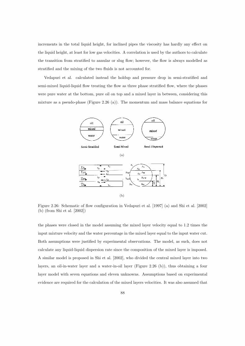
increments in the total liquid height, for inclined pipes the viscosity has hardly any effect on
the liquid height, at least for low gas velocities. A correlation is used by the authors to calculate
the transition from stratified to annular or slug flow; however, the flow is always modelled as
stratified and the mixing of the two fluids is not accounted for.
Vedapuri et al. calculated instead the holdup and pressure drop in semi-stratified and
semi-mixed liquid-liquid flow treating the flow as three phase stratified flow, where the phases
were pure water at the bottom, pure oil on top and a mixed layer in between, considering this
mixture as a pseudo-phase (Figure 2.26 (a)). The momentum and mass balance equations for
(a)
(b)
Figure 2.26: Schematic of flow configuration in Vedapuri et al. [1997] (a) and Shi et al. [2002](b) (from Shi et al. [2002])
the phases were closed in the model assuming the mixed layer velocity equal to 1.2 times the
input mixture velocity and the water percentage in the mixed layer equal to the input water cut.
Both assumptions were justified by experimental observations. The model, as such, does not
calculate any liquid-liquid dispersion rate since the composition of the mixed layer is imposed.
A similar model is proposed in Shi et al. [2002], who divided the central mixed layer into two
layers, an oil-in-water layer and a water-in-oil layer (Figure 2.26 (b)), thus obtaining a four
layer model with seven equations and eleven unknowns. Assumptions based on experimental
evidence are required for the calculation of the mixed layers velocities. It was also assumed that
88

the transition from oil in water to water in oil along the vertical coordinate occurred at 45%
local water cut (valid, of course, only for the system studied by the authors) and the two kind
of dispersion were homogeneous with representative mixture density and viscosity, the latter
being evaluated with a model based on Brinkman’s model.
Jayawardena et al. [2000] modelled oil-water flow as two layers flowing on top of each
other, pure water on the bottom and an oil-water mixed layer on top. Momentum equations
were applied to each layer using average densities and viscosities. The model requires closure
relationships to calculate the oil content in the dispersion. The authors proposed three possible
closures: the simplest is the direct measure of the pure water layer height; however direct
measurements are not possible in most of the cases. The second method consists in varying the
oil content until the predicted pressure gradient matches the experimental pressure gradient.
The third proposed method attempts to correlate the flow rate of the pure water at the bottom
to the flow rate of the dispersion on top by assuming that the ratio of the two flow rates is
proportional to the ratio of the cross sectional areas occupied by each layer. The prediction of
the oil content in the mixed layer is a major weakness of the model.
Lovick [2004] presented a development of the two fluid model (Taitel and Dukler [1976])
where oil and water were modelled as two layers with entrainment from each layer into the
other. Therefore, the model accounts for an oil continuous phase with entrained water that
flows on top and a water continuous phase with entrained oil that flows at the bottom of the
pipe. A one-dimensional momentum balance equation is solved for each phase, with appropriate
closure models for the phases densities and viscosities and for the liquid-wall and liquid-liquid
interfacial friction factors. Calculation were performed twice, first assuming a flat interface
between the fluids and then introducing the interfacial curvature in the calculation, where the
value of the curvature was obtained from the experimental data.
A two fluid momentum balance was used also by Valle [2000], who analysed the force acting
on dispersed drops to derive expressions for the drop entrainment and deposition. Valle treated
the onset of entrainment with the harmonic stability theory already proposed in Trallero [1995].
Once drops are entrained, three forces are assumed to act on them, namely the gravity force,
the drag and the driving force due to turbulence. Valle proposed that dispersion of entrained
drops in a layer occurs when the driving turbulent force prevails over the gravity force. The
89

entrainment rate formula derived by Valle is expressed in the form:
E = C1dinit
λ
(〈v′+2〉u2
∗ −23dinit
|ρc − ρd|ρc
g cos ϑ
)(2.51)
where λ is the interfacial wavelength, dinit is the drop diameter calculated with Hinze’s expres-
sion and 〈v′+2〉 is the dimensionless cross sectional averaged velocity fluctuation, assumed by
Valle equal to 1.44 but with the recommendation of further investigation. The parameter C1
in Equation (2.51) lumps together several constants and no exact expression for this parameter
is proposed by Valle, who sets C1 = 0.1 based on experimental observations.
For the derivation of the deposition rate, Valle again performed a balance of all the forces
acting on the dispersed drops, namely gravity, drag, lift, virtual mass and Basset forces. To
this balance, also the displacement force is added, which accounts for the force required to
drain the film between a drop and the layer interface as the drop approaches it. The final
stage of deposition, that is the coalescence of the approaching droplets on the layer surface, is
approximated by Valle with the model by Charles and Mason [1960].
Valle extended his work to three-phase liquid-liquid-gas flow also and accounted for the
presence of gas bubbles entrained inside the liquid body. Correlations were used to determine
the transition between the basic flow patterns accounted in his model (stratified, annular,
bubbly and slug flow).
Another approach to the calculation of oil and water entrainment is proposed in Al-Wahaibi
[2006] for a framework similar to those of Lovick [2004] and Valle [2000] (two layers flowing on
top of each other, each one with a continuous and dispersed phase and mass exchange between
the layers). The model in Al-Wahaibi [2006] assumes equilibrium between deposition and
entrainment rate. The entrainment rate follows the model proposed in Holowach et al. [2002];
it is assumed that the drop formation mechanism is connected to the formation of interfacial
waves between the fluids and drops detach from the crest of the waves as a consequence of the
difference in velocity between the layers. Critical quantities to be calculated are the numbers
of waves in a control volume, the drop entrainment time and the volume entrained from each
wave. Oil and water deposition rates are calculated by use of empirical correlations based on
the oil and water superficial velocities and friction velocity.
90

Bonizzi and Issa [2003] performed the simulation of three-phase oil-water-gas slug flow in
pipelines within the framework of the two-fluids model already validated for two-phase gas-liquid
flow. The two-fluids model was applied to the gas and the liquid phase, wherein the liquid phase
was considered as the ensemble of water and oil regardless of the flow pattern. The total liquid
mass required the solution of one single momentum equation for the calculation of the mixture
velocity. For stratified flow, a correlation was used to evaluate the slip velocity between the
liquid phases; accordingly, approximated oil and water velocities were calculated without adding
other momentum equations to the set of equations of the model. The dispersion rate of one liquid
into the other was not calculated; rather, only two flow patterns were accounted for: stratified
and fully dispersed flow. The transition from one flow pattern to the other was assumed to
Figure 2.27: Three-phase slug flow. White = gas, Red = oil, Blue = water. (Bonizzi and Issa[2003])
occur abruptly (see Figure 2.27) and was determined using the criterion proposed in Brauner
and Maron [1992] while the continuous phase in fully dispersed flow and phase inversion where
determined applying Decarre and Fabre [1997] criteria. No attempt was made to reproduce
analytically the dispersion process of one phase into the other. The model was able to predict
three-phase slug flow with reasonable agreement between calculation and experimental pressure
losses and slug frequencies.
Chesters and Issa [2004] proposed a mathematical model to describe the evolution of phase
inversion processes in two-fluid systems. The model is based on the calculation of the dis-
persed phase fraction and the fraction of continuous phase ingested by the dispersed phase as
droplets-in-drops (secondary dispersion). The model accounts for the presence of a fluctuating
inversion front of finite thickness between the two dispersion types. The work as such provides a
91

framework that has to be completed with suitable source terms for the equations of the model,
a continuity equation for the continuous phase, a momentum equation for the dispersed and
continuous phases, a turbulence model and interfacial area. Although the model was formu-
lated for multidimensional flow, it provides elements that could be adapted in this thesis to
one-dimensional situations.
2.9 Summary
Literature concerning the main features of two-phase liquid/liquid flow in pipelines was
reviewed in this chapter. Attention was paid to the spatial distribution of the two phases (flow
pattern), to the factors influencing the flow patterns and to the pressure gradient. Mixing
processes between the phases resulting in the formation of mixtures with drops of one phase
dispersed into the other phase were identified. A review of the models to calculate the maximum
drop diameter was presented, with some notes on the studies on drop size distribution, drop
breakup and coalescence among drops. The interactions between the dispersed phase drops
may lead to phase inversion with continuous and dispersed phase exchanging roles. This process
involves dramatic changes in the mixture properties and is often signalled by an increase in the
flow pressure losses.
Two-phase liquid-liquid is often encountered in industrial processes and analytical tools
are required to study the flow computationally and predict the flow pattern and the pressure
losses, dispersion process of the two phases and phase inversion. Because of the complexity of
the phenomena involved the modelling of liquid-liquid flow is a hard task to accomplish. The
review of the existing computational model showed the deficiencies of each model and the need
for further improvements. The development of a model for liquid-liquid immiscible flow is the
subject of next chapter, where a one-dimensional model is proposed in order to simulate the
dispersion of the phases in pipe flow and phase inversion.
92

Chapter 3
Present approach for liquid-liquid
dispersions in pipelines
3.1 General description of the model
In this chapter a model will be proposed for the analytical description of the flow of two
immiscible liquids, such as oil and water, in pipes. The model is proposed as a tool for the
description of the changes in the flow properties (viscosity, density, pressure losses) spatially and
temporally. This is achieved by modelling the physical phenomena usually encountered in oil-
water flow, namely the formation of emulsions and dispersions. The dependency of the phase
velocities and phase distribution on space and time are typically obtained through solution
of partial differential equations. The complexity of the physics involved would require the
solution of 3D equations. However, the one-dimensional approximation is often applied to pipe
flow since the relevant phenomena occur along the pipe axis while the two other coordinate do
not assume particular importance. However, the one-dimensional approach inevitably implies
the calculation of averages across the section. The first task in liquid-liquid one-dimensional
modelling is, therefore, to create a suitable simplified framework for the phenomena described in
chapter 2; then, equations may be proposed to calculate the quantities within that framework.
The flow patterns described in section 2.2 are differentiated by the distribution of the two phases
93

across the pipe section; but a one-dimensional approach cannot effectively account for all the
possible distributions of the phases across the section (namely the flow pattern). Therefore, the
flow patterns described in section 2.2 must be reduced to a simple scheme of basic configurations
easily dealt with. The most natural choice is to classify the flow pattern into fully stratified
with negligible amount of dispersion, stratified dispersed flow and fully dispersed flow. As such,
for stratified and partially dispersed flow, the approach used in the model for the description
of oil and water flow is placed in the category of the dual continuous flow, where each phase
retains its continuity while dispersion of one fluid into the other appears under the form of
dispersed droplets (Lovick [2004], Al-Wahaibi [2006]). For the description of the flow, the
phases are conceived as flowing within two layers, both of which composed of a continuous
and a dispersed phase. Therefore, the bottom layer will be described as a layer where the
heavier phase (namely, water) flows as the continuous phase while the lighter phase (namely
oil) forms the dispersed phase. Vice versa, the layer at the top is modelled as a lighter continuous
phase while the heavier phase is dispersed as drops inside the former. As such, each layer is
regarded as a mixture, for which it is possible to determine the composition by calculating the
percentage of continuous and dispersed phases and derive average properties (namely, mixture
density and mixture viscosity). The two-layer configuration is schematically represented in
picture 3.1 in a typical situation where both layers are emulsions of one phase dispersed into
the other. When no dispersion occurs between the fluids, the flow is fully stratified with pure
liquids flowing in each layer. Conversely, the transition from stratified-dispersed flow to fully
dispersed flow is supposed to happen as described by Nadler and Mewes [1997], with phase
inversion happening inside either of the layers. Mass exchange is allowed between the layers in
the form of entrainment from the continuous phase of one layer to the dispersed phase of the
other (positive source term for dispersed phase) and deposition of dispersed phase drops onto
the other layer (negative source term for the dispersed phase), as schematically represented in
Figure 3.2.
Four variables are introduced with the aim of calculating the fraction of oil and water inside
each layer:
• αw (x, t) - fraction of water in the bottom layer
94

Figure 3.1: Layers of oil in water and water in oil flowing inside a pipe
• βo (x, t) - fraction of oil in the bottom layer
• αo (x, t) - fraction of oil in the top layer
• βw (x, t) - fraction of water in the top layer
The fractions of water and oil in the bottom layer (αw and βo) give the total liquid fraction
in the lower layer while the upper layer faction is given by the summation of αo and βw. In
view of the one-dimensional approximation used, each of the aforementioned quantity should
be suitably calculated as area-averaged quantities, as suggested, among others, by Ishii and
Mishima [1984]. In general, if Υk denotes a function of phase k, the area-averaged value of Υk
will be calculated as:
Υk =
∫Ak
ΥkdA∫Ak
dA=
∫Ak
ΥkdA
αkA, (3.1)
where Ak is the area occupied by phase k. It is supposed that each dispersed phase is homoge-
neously distributed in the layer, i.e. high mixing efficiency is assumed. Moreover, it is supposed
that the dispersed phase in each layer moves at the same velocity with the continuous phase,
that is to say no-slip is assumed between the continuous and dispersed phases, although this is
not an essential assumption for the model. Alternatively, one could apply the drift flux model
95

Figure 3.2: Entrainment and deposition scheme. Dw = water drops deposition, Ew = waterdrops entrainment, Do = oil drops deposition, Eo = oil drops entrainment
(developed, among the others by Ishii [1975] and Wallis [1969] ) to evaluate the velocity of the
continuous and dispersed phases in each layer.
The dispersed phase drops will be supposed to all have the same size, set equal to the
mean Sauter diameter d32. Obviously, the value of the mean Sauter diameter will depend on
the local flow conditions and therefore will be a function of space and time. The choice of a
uniform distribution has the advantage of avoiding the calculation of break-up and coalescence
rates and the solution of population-balance model equations. The inclusion of secondary
ingested droplets will not be accounted for; further improvements of the model to account for
secondary dispersion will be discussed in the chapter on future work. It will be assumed that
heat exchange between the fluids and the pipe wall is negligible (isothermal flow) and no energy
equation for the phases will therefore be required. The effect of surfactants and contaminants
is not accounted for. For convenience, the two immiscible phases will be referred to as oil (the
lighter) and water (the heavier) without the model losing generality.
3.2 Model equations
The scalar quantities introduced in the previous section (αw, βo, αo, βw) are time and space
dependent and each requires the solution of a transport equation. The continuity equations for
96

each quantity take the form:
∂ (ρwαw)∂t
+∂ (ρwulαw)
∂x=
SαwSi
A(3.2a)
∂ (ρwβw)∂t
+∂ (ρwuuβw)
∂x=
SβwSi
A(3.2b)
∂ (ρoαo)∂t
+∂ (ρoulαo)
∂x=
SαoSi
A(3.2c)
∂ (ρoβo)∂t
+∂ (ρoulβo)
∂x=
SβoSi
A, (3.2d)
where the subscript u and l stand for lower and upper layer respectively, Sλ is the source term
for each associated phase fraction and Si is the interfacial width. The solution of Equations
(3.2) is possible when a suitable set of initial and boundary condition are specified. The sum of
the four quantities defined above has to be equal to the total liquid fraction, which is unity for
two-phase flow. Therefore, only the calculation of three of the four quantities above is strictly
required, the forth being obtained as the difference from 1 (two-phase flow) or the mixture
fraction (three-phase flow). In what follows, only αw, βw and βo will be considered, leaving the
amount of oil in the upper layer to be obtained from the others. The source term on the RHS
of the continuity equations (3.2) for the two dispersed phases is responsible for the liquid-liquid
mixing process since it caters for the variations of the dispersed phase fractions within the two
continuous phases. It takes the form:
Sβw = water entrainment rate− water deposition rate
Sβo = oil entrainment rate− oil deposition rate
Sαw = −Sβw
Sαo = −Sβo .
The first component of the source term (Entrainment) is responsible for the generation of
droplets from the continuous phase of one layer to augment the dispersed phase of the other
layer. The second term (Deposition), on the other hand, accounts for the deposition of dispersed
phase drops across the interface between the layers that are absorbed by the continuous phase
of the receiving layer.
97

The process of mutual dispersion of two immiscible liquids is still not clearly understood
and therefore the available literature does not offer a validated model that caters for all the
aspects of this complex phenomenon. In the present work, it has been chosen to make use of the
knowledge and experience gained in the field of gas-liquid flow modelling and to adapt models
developed for gas-liquid dispersion to liquid-liquid dispersion. The gas - liquid models selected
to be used for the liquid - liquid dispersion are modified so as to account for the different
aspects of the two-liquid flow that are not encountered in the gas - liquid flow. Entrainment
and deposition rates will be treated in details in sections 3.3 and 3.4 respectively.
The solution of Equations (3.2) requires knowledge of the velocity in each layer, which is the
same for both continuous and dispersed phase when assuming no-slip. The layer velocities can
be calculated as solution of the equations of the two-fluid model, developed among others by
Ishii [1975]. In its general formulation, the two-fluid model describes the flow of two fluids by
solving three dimensional equations (Ishii [1975], Prosperetti and Jones [1984]). A simplified
one-dimensional version of the model is proposed, for example, in Taitel and Dukler [1976],
Ardron [1980], Ishii and Mishima [1984] and Barnea and Taitel [1994] based on the area-averages
of the quantities. The hypothesis will be made, that the mixture in each layer behaves as a
homogeneous fluid characterized by an area-average density and an appropriately calculated
viscosity. The two-fluid model is based on the solution of two sets of equations, one for each
phase, comprising a continuity equation, a momentum equation and an energy equation. In
the present work, therefore, a continuity and a momentum equation should be solved for the
mixture in each layer, giving the following set of equations:
Upper layer continuity equation
∂ (ρuαu)∂t
+∂ (ρuuuαu)
∂x= Sαu (3.3)
Lower layer continuity equation
∂ (ρlαl)∂t
+∂ (ρlulαl)
∂x= Sαl
(3.4)
98

Upper layer momentum equation
∂ (ρuαuuu)∂t
+∂
(ρuαuu2
u
)
∂x= −αu
∂pi
∂x− αuρug
∂hi
∂xcos γ+
− g cos γ∂ρu
∂x
αuhi − 2R
π
[2π − ϑi
4+
sin ϑi
4+
13
sin3 ϑi
2
]+
− αuρug sin γ − τWuSu
A− τiSi
A
(3.5)
Lower layer momentum equation
∂ (ρlαlul)∂t
+∂
(ρlαlu
2l
)
∂x= −αl
∂pi
∂x− αlρlg
∂hi
∂xcos γ+
− g cos γ∂ρl
∂x
αlhi − 2R
π
[ϑi
4− sin ϑi
4− 1
3sin3 ϑi
2
]+
− αlρlg sin γ − τWlSl
A+
τiSi
A
(3.6)
In Equations (3.3), (3.4), (3.5), (3.6), x and t represent the spatial and temporal variable
respectively, pi is the interfacial pressure, hi is the height of the lower layer, ϑi the angle
determined by the interface between the layers (fig 3.3), R is the pipe radius, γ is the pipe
inclination, A the pipe cross section, τWk is the shear stress between the wall and layer k, Sk
the layer-wall wetted perimeter and τi and Si are the interfacial shear stress and the interfacial
cord respectively.
The term depending on the density derivative in Equations (3.5) and (3.6) comes from
the derivation of the hydrostatic pressure term, as reported in Appendix A. Obviously, if the
composition of the layers does not change, the layer density remains constant and the density
derivative terms disappear.
The layer fractions αu and αl in Equations (3.3) - (3.6) are related to the continuous and
dispersed fractions inside each layer by the simple relations:
αu = αo + βw
αl = αw + βo,
(3.7)
99

Figure 3.3: Two phase flow variables
and the layer densities ρu and ρl are calculated with:
ρu =αoρo + βwρw
αo + βw
ρl =αwρw + βoρo
αw + βo.
(3.8)
In the momentum equations (3.6) and (3.5) the momentum transfer between the layer associated
with the mass exchange is neglected.
By substituting Equations (3.7) and (3.8) into Equations (3.3) and (3.4), one obtains that
the continuity equations for αu and αl can be easily derived from the continuity equations (3.2)
and Sαu = Sαo +Sβw , Sαl= Sαw +Sβo . The equations to be solved for the two-fluid model are
therefore (3.2), (3.5) and (3.6). The two momentum equations require closure relations for the
calculation of the liquid-wall and liquid-liquid interfacial shear stresses; the continuity equations
(3.2), instead, require closure model for the calculation of the entrainment and deposition rate.
The closure models used in the present work for the calculation of the friction factors will be
detailed briefly in the following section while the source term for the continuity equations will
be the subject of discussion in sections 3.3 and 3.4.
100

3.2.1 Closure models
The body forces acting on the two layers are represented by the terms −τWuSu
A, −τWlSl
A,
τiSi
A, −αuρug sin β, −αlρlg sin β, where τWu, τWl and τi are the upper layer-wall shear stress,
the lower layer-wall shear stress and the interfacial shear stress. The shear stresses are commonly
related to the dynamic pressure by expressions of the form:
τWk =12ρkfkuk|uk|, (3.9)
for the liquid-wall shear stress and
τi =12ρfiurel|urel|, (3.10)
for the interfacial shear stress.
The parameters fk and fi represent the liquid-wall and the interfacial friction factors re-
spectively while urel = uu−ul is the relative velocity between the two layers. Many correlations
are available in the literature for the calculation of the friction factors; in this work, the corre-
lations proposed by Blasius and Zigrang & Sylvester (Equations (3.11) and (3.12) respectively)
are adopted and the results are examined:
f =
0.079Re−0.25k for Rek < 105
0.046Re0.2k for Rek > 105
(3.11)
1√f
= −2 log
er/d
3.7− 4.518
Reklog
[6.9Rek
+(
er/d
3.7
)1.1]
(3.12)
The parameter er in Equation (3.12) is the roughness of the internal wall of the pipe. Equations
(3.11) and (3.12) provide the liquid-wall friction factor in turbulent flow; for laminar flow, the
well-known relation
fk =16
Rek(3.13)
101

is used. The Reynolds number Rek is based on the properties of layer k as
Rek =ρkDkuk
µk, (3.14)
being Dk the hydraulic diameter of the layer.
Additionally, the applicability of the correlation by Hand [1991] and Spedding and Hand
[1997] is tested against experimental data, following the investigations of Rippiner [1998] and
Issa and Kempf [2003]. Rippiner [1998] performed extensive comparisons between the corre-
lations available for gas-liquid flow in order to determine the best combination of gas-wall,
liquid-wall and liquid-gas friction factor correlations. The task of this investigation was the
prediction of the gas-liquid slug flow regime, with attention being paid to slug characteris-
tics. The Hand correlation was found to be the best choice for the liquid-wall friction factor.
Bonizzi [2003] applied the findings of Rippiner to the study of three-phase gas-oil-water flow
in pipelines, calculating the oil-wall and water-wall friction factors in stratified flow applying
the Hand’s correlation to both fluids. In the present study Hand’s correlation is tested so that
three-phase slug flow would reduce naturally to two-phase liquid-liquid flow for gas fractions
decreasing to zero. Hand’s correlation is expressed in the form:
fk =24
ReSk
(3.15)
for laminar flow and as:
fk = 0.0262(αkReS
k
)−0.0139(3.16)
for turbulent flow. The Reynolds number ReSk that appears in Equations (3.15) and (3.16)
is calculated from the layer superficial velocity and it is based on the layer averaged density
and layer viscosity, using again the assumption that the mixture in each layer behaves as a
homogeneous fluid with appropriate properties:
ReSk =
ρkDUk
µk, (3.17)
where ρk is calculated according to Equations (3.8), D is the pipe diameter and µk is the layer
102

viscosity. The transition from laminar to turbulent flow is determined from a Reynolds number
based on the actual velocity of the fluid:
Rek =ρkDkuk
µk. (3.18)
The flow is assumed to be laminar when Rek < 2100; otherwise, turbulent flow is assumed to
occur. The hydraulic diameter Dk that appears in (3.18) is calculated from the usual expression
Dk =4 × area occupied by the fluid
wetted perimeter.
Commonly, the faster phase is assumed to flow in an enclosed channel and, therefore, the
wetted perimeter is obtained from the phase-wall wetted perimeter plus the interfacial chord.
The slower phase, instead, is assumed to flow in an open channel and the wetted perimeter is
assumed to be the phase-wall contact surface only. Therefore:
Dk =4αkA
SWk + Si(3.19a)
Dk =4αkA
SWk, (3.19b)
where k is the faster phase. This approximation is widely used when dealing with two-phase
gas-liquid flow, in which case the gas velocity is usually much higher than the liquid velocity
and the approximation of the gas as flowing in an enclosed channel is acceptable. For liquid-
liquid flow, velocities do not differ as much as in gas-liquid flow and are often of the same order,
and Brauner et al. [1998] proposed to exclude the interfacial chord from the hydraulic diameter
for both phases when the two liquid velocities are comparable, so yielding Dk =4αkA
SWk
and
Dk =4αkA
SWk. The mixture viscosity required for the calculation of the Reynolds number is
provided by Brinkman [1952] and Roscoe [1953] (Equation (2.16)). Although there exist more
advanced models, the formula does not require tunable constants and offer the advantage of
generality and simplicity.
Taitel et al. [1995] assumed fi equal to 0.014 or equal to the oil-wall friction factor whenever
the latter was higher than 0.014. A similar approach for the calculation of fi is adopted in the
103

present work and the interfacial friction factor is calculated according to:
fi = maxfWk, 0.014
, (3.20)
where, as before, the subscript k refers to the faster of the two layers. Consistently, the density
in Equation (3.10) is taken as the density of the faster layer, giving:
τi =12ρkfiurel|urel|. (3.21)
Closure relations are needed also for the phase inversion events in each layer. The criteria
for phase inversion have to be applied to each layer: a comparison is made between the amount
of oil in each layer εo and the critical oil fraction ε0crit; when the condition εo > ε0
crit is satisfied,
oil is assumed to be the continuous phase. Bonizzi [2003] performed a comparison between
the criteria for phase inversion proposed by Arirachakaran et al. [1989], Decarre and Fabre
[1997], Brauner and Ullmann [2002], Nadler and Mewes [1995b] and Odozi [2000]. The aim
of Bonizzi’s work was to choose a criterion for phase inversion in three-phase oil/water/gas
slug flow; the predictions of the correlations listed above were compared against experimental
data and the criterion with the smallest error in predicting the experimental continuous phase
was identified. Although the criteria of Decarre and Fabre [1997] were developed for agitated
vessels, Bonizzi showed that they could predict with a smaller error the continuous phase for
the pipe flow data examined. Those criteria were therefore chosen and applied to three-phase
slug flow. Bonizzi’s work had the limitation that all the experimental data examined were in
the turbulent flow region; moreover, the criteria were tested for three-phase slug flow and the
presence of gas in the liquid mass, not accounted for in the criteria, might have influenced the
results of the comparisons. Nevertheless, as it was not possible to perform a similar comparison
against experimental data in the present work, the criteria of Decarre and Fabre were adopted
to determine the phase inversion point in oil-water flow. The criteria of Decarre and Fabre
depend on the flow regime before and after the occurrence of phase inversion; three cases were
considered by Decarre and Fabre, namely laminar or turbulent flow both before and after phase
inversion and the case of laminar flow with oil continuous phase and turbulent flow with water
104

continuous phase. The transition from laminar water continuous flow to turbulent oil continuous
was not examined as it is considered to be unlikely since it has not been commonly observed.
The criteria derived are therefore:
• For laminar flow before and after phase inversion
λw =
1 +
(µw
µo
)2/3−1
(3.22)
• For turbulent flow before and after phase inversion
λw =
1 +
(µw
µo
)1/14 (ρw
ρo
)5/14−1
(3.23)
• For turbulent flow when water is the continuous phase and laminar flow when oil is the
continuous phase
(1− λw)7/5
λw=
0.1451.15 · 23/5
(σfWw)2/5 (Dρw)3/5 U1/5M
µ5/6o µ
1/6w
. (3.24)
As a first approximation, it was chosen to consider a uniform size distribution for the
dispersed phase droplets, namely the mean Sauter diameter. The calculation of the mean
Sauter diameter was performed starting from the maximum stable drop size in a turbulent
field. The expressions proposed by Brauner [2001] (Equations (2.33) and (2.36)) were adopted
for the maximum drop size and, assuming a log-normal distribution in equilibrium conditions
according to the suggestions of Simmons and Azzopardi [2001], the mean Sauter diameter was
obtained from the maximum stable diameter according to (2.42).
As such, the model requires the solution of three continuity equations (Equations (3.2)) and
two momentum equations (Equations (3.5) and (3.6)) and all the equations are closed by source
terms and closure models. The number of differential equations required can be reduced if it
is observed that the flowing incompressible fluids have to satisfy the continuity equation for
the global mixture (all the water plus all the oil) that enters the pipe. From the definition of
mixture density and mixture velocity (derived from the definition of centre of mass velocity),
it follows that:
αMρMuM = (αwρw + βoρo)ul + (αoρo + βwρw)uu, (3.25)
where αM is the total mixture fraction, which is equal to 1 for liquid-liquid flow. Introducing
105

the quantity cl as:
cl =αwρw + βoρo
αMρM, (3.26)
Equation (3.25) becomes:
uM = clul + (1− cl)uu. (3.27)
Furthermore, introducing the slip velocity us between the layers as:
us = uu − ul, (3.28)
simple calculations yield:
uu = uM + clus (3.29a)
ul = uM + (1− cl) us. (3.29b)
Therefore, knowing the mixture velocity from continuity and the slip velocity between the
layers, the layer velocity can be immediately calculated approximately without solving the
layer momentum equation. The calculation of the slip velocity can be approximated as done
in Bonizzi and Issa [2003]. Considering a steady state regime where both temporal and spatial
derivatives vanish and neglecting static head and inertia terms, Equations (3.5) and (3.6) reduce
to:
• Upper layer momentum equation
0 = −αu∂pj
∂x−−αuρug sin γ − τWuSu
A− τiSi
A(3.30)
• Lower layer momentum equation
0 = −αl∂pi
∂x− αlρlg sin γ − τWlSl
A+
τiSi
A(3.31)
By eliminating the pressure gradient between the equations, one obtains
τWlSl
αlA− τWuSu
αuA− τiSi
A
(1αu
+1αl
)+ (ρl − ρu) g sin γ = 0 (3.32)
Equation (3.32) contains the slip velocity in each shear stress, since the layer velocities are
106
calculated according to (3.29); it has therefore to be solved numerically in order to obtain the
slip velocity. An approximate solution of the two-phase incompressible flow can be obtained
deriving the layer velocities from Equation (3.29) and Equation (3.32) and inserting them into
Equations (3.2) (Figure D-1 in Appendix D). Figure D-2, instead, shows the implicit solution
procedure of the equations of the model when the layer velocities are obtained by solving the
momentum equations (3.5) and (3.6).
3.3 Entrainment models
Equations (3.2) requires the specification of the mass exchange between the layers in the
form of entrainment and deposition rates. Entrainment is a complex phenomenon that involves
processes at the liquid interface leading to the appearance of interfacial waves and fingers
protruding from one layer into the other. From these protruding structures, filaments are
detached, which may be carried away from the interface, thereby increasing the dispersed phase
fraction. For fluids with different densities with the lighter fluid flowing on top, the interfacial
instabilities are often referred to as Kelvin-Helmholtz instabilities. A mechanistic approach for
the calculation of the entrainment rate in gas-liquid vertical flow was proposed in Holowach
et al. [2002]. The model applies a force balance (gravity force, drag force and surface tension
force) to the interfacial waves; the number of waves Nwaves in a control volume is calculated
and together with the volume VE entrained from the crest of each wave both give the entrained
volume fraction per unit time and unit volume in the form:
RE =VEρk,ENwaves
Aiτe, (3.33)
where Ai is the interfacial area in the control volume and τe is the entrainment time. A mech-
anist model such as the one mentioned above offers the advantage of generality and would be
applicable in principle to liquid-liquid systems. However, the drawback is significant complexity
and the need for numerous calculations.
Two models will be proposed for the calculation of the entrainment and deposition rate.
It is noted here that experimental data available do not provide the value of entrainment and
107

deposition, but the equilibrium concentration of the dispersed phase in fully developed flow,
when the deposition rate is equal to the entrainment rate. Since no data are available in the
region of developing flow, entrainment and deposition rate correlations were tested against fully
developed flow conditions only.
3.3.1 Entrainment model based on de Bertodano et al. [1998] corre-
lation
An alternative to mechanistic models is offered by correlations based on dimensionless num-
bers. Referring again to the analogy between gas-liquid and liquid-liquid flow, the correlation
of de Bertodano et al. [1998] was modified so as to apply to the case of two immiscible liquids
flowing in a horizontal conduit. The correlation was originally developed for entrainment in
gas-liquid vertical flow, in the form:
RED
µfilm=
4.47× 10⁻⁷
[Weg
(√ρfilm − ρg
ρg
)(Re−Recrit)
]0.925 (µg
µfilm
)0.26
for Re > Recrit
0 for Re < Recrit
(3.34)
where Re is the Reynolds number relative to the liquid film wetting the internal wall of the
pipe and Weg =ρgu
2gD
σw/gis the Weber number calculated from the gas core velocity. The
value of Recrit is used as a threshold for the start of the entrainment process and is tuned
from experimental data. The correlation is linked to the Kelvin-Helmholtz instabilities at the
interface; assuming that the same kind of instabilities are responsible for the production of
dispersion at interface, the correlation was used as a starting point for the calculation of the
liquid entrainment rate from one layer into the other. It was necessary to modify Equation
(3.34) to adapt the correlation from the annular concentric geometry to the stratified layers
geometry. The Weber number was related to the slip velocity between the two layers, giving
We =ρEu2
sD
σw/o. (3.35)
The slip velocity was adopted instead of the velocity of the entraining phase, thus relating
entrainment to the interface shear stress. In the case of gas/liquid flow, the gas velocity is
108

usually much higher than the liquid film velocity and the slip velocity between gas and liquid
may be approximated by the gas velocity (us ∼ ug); Equation (3.35) would therefore return
the expression for the Weber number Weg used in Equation (3.34). As the Reynolds number
Re was calculated in the original correlation from the values of velocity, viscosity and hydraulic
diameter of the entrained phase, by analogy here it was derived from velocity, viscosity and
hydraulic diameter of the entrained layer. The value of the constant that determines the order
of magnitude of the term was tuned against experimental flow maps to match the experimental
liquid/liquid flow regimes and the value of 17.1 · 10−5 was obtained. In Figure 3.4 the slip
velocity us as calculated from the solution of (3.28) is represented for five different mixture
velocities as a function of the input water cut, for pure liquids and assuming flat interface
between the fluids. Calculations, in particular, are performed for the oil used in the work of
Elseth [2001], but similar results can be easily obtained for different oil properties.
0 0.1 0.2 0.3 0.4 0.5 0.6 0.7 0.8 0.9 1input water fraction
-2
-1.5
-1
-0.5
0
0.5
1
1.5
2
slip
vel
ocity
[m
/s]
mixture velocity = 1.0 m/smixture velocity = 1.5 m/smixture velocity = 2.0 m/smixture velocity = 2.5 m/smixture velocity = 3.0 m/s
Figure 3.4: Slip velocity vs water cut at different mixture velocities, flat interface and pureliquids
109

Figure 3.4 clearly shows that the slip velocity assumes high values for small or high input
water fraction while for intermediate water cut its value is relatively small and becomes zero
at one point. This is a point were no entrainment would be predicted, as the Weber number
in both equations (3.38) and (3.39) would be zero and the flow would remain stratified even
at high mixture velocities. The conditions for no-slip between the layers can be inferred from
Equation (3.32): by imposing us = 0, it reduces to:
τWlSl
αlA− τWuSu
αuA+ (ρl − ρu) g sin γ = 0, (3.36)
and, therefore, the minimum value of the entrainment rate will depend on the properties of
the fluid, on the characteristics of the flow and on the geometry of the pipe. Physically, for
sufficiently high mixture velocities fully dispersed flow can result regardless of the water cut, as
small instabilities may grow becoming interfacial waves, leading to the production of a dispersed
phase. To account for the formation of such instabilities, the slip velocity in the Weber number
in Equation (3.35) was replaced with a linear combination of the slip velocity and the difference
in the friction velocity of the two layers, obtaining:
We =ρE (|us|+ c1|4u∗|)2 Di
σw/o. (3.37)
where 4u∗ = u∗,l − u∗,u and the value of c1 was tuned to 2.15. Figure 3.5 shows how the
quantity |us|+ c1|4u∗| changes against the input water fraction for five different velocities. As
in Figure 3.4, there is a minimum corresponding to limited entrainment between the phases;
however, this minimum is not zero and the entrainment term does not vanish.
With the modifications discussed before, Equation (3.34) then becomes:
RED
µw=
17.1 · 10−5
[We
(√ρw − ρo
ρo
)(Rew −Rew
crit)]0.925 (
µo
µw
)0.26
for Rew > Recrit
0 for Rew < Recrit
(3.38)
110

0 0,1 0,2 0,3 0,4 0,5 0,6 0,7 0,8 0,9 1input water fraction
0
0,4
0,8
1,2
1,6
2
abs(
us)+
c1ab
s(u*
o-u*
w)
mixture velocity = 1.0 m/smixture velocity = 1.5 m/smixture velocity = 2.0 m/smixture velocity = 2.5 m/smixture velocity = 3.0 m/s
Figure 3.5: |us| + c1|4u∗| vs inlet water cut at different mixture velocities, flat interface andpure liquids.
for the entrainment of water into oil and
RED
µo=
17.1 · 10−5
[We
(√ρw − ρo
ρw
)(Reo −Reo
crit)]0.925 (
µw
µo
)0.26
for Reo > Recrit
0 for Reo < Recrit
(3.39)
for the entrainment of oil into water. The critical values of the Reynolds numbers Recrit were
obtained from the corresponding values in the Hussain [2004] flow map corresponding to the
transition at low mixture velocities between stratified and partially dispersed flow. The values
determined were 7000 for water and 3300 for oil.
The entrainment rates calculated by Equations (3.38) and (3.39) are plotted in Figure 3.6
for different mixture velocities and as a function of the input water fraction.
The entrainment rates in Figure 3.6 are clearly non symmetrical; for low input water fraction
111
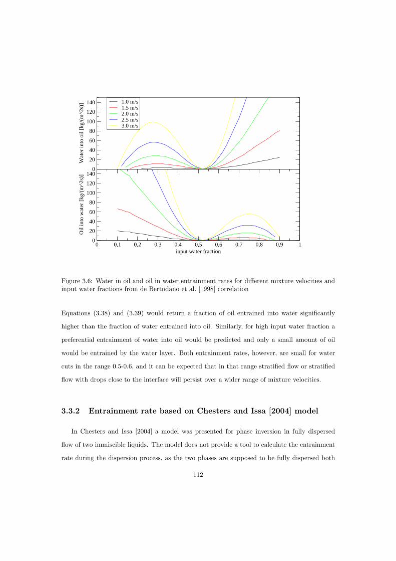
0
20
40
60
80
100
120
140
Wat
er in
to o
il [k
g/(m
^2s)
] 1.0 m/s1.5 m/s2.0 m/s2.5 m/s3.0 m/s
0 0,1 0,2 0,3 0,4 0,5 0,6 0,7 0,8 0,9 1input water fraction
0
20
40
60
80
100
120
140
Oil
into
wat
er [
kg/(
m^2
s)]
Figure 3.6: Water in oil and oil in water entrainment rates for different mixture velocities andinput water fractions from de Bertodano et al. [1998] correlation
Equations (3.38) and (3.39) would return a fraction of oil entrained into water significantly
higher than the fraction of water entrained into oil. Similarly, for high input water fraction a
preferential entrainment of water into oil would be predicted and only a small amount of oil
would be entrained by the water layer. Both entrainment rates, however, are small for water
cuts in the range 0.5-0.6, and it can be expected that in that range stratified flow or stratified
flow with drops close to the interface will persist over a wider range of mixture velocities.
3.3.2 Entrainment rate based on Chesters and Issa [2004] model
In Chesters and Issa [2004] a model was presented for phase inversion in fully dispersed
flow of two immiscible liquids. The model does not provide a tool to calculate the entrainment
rate during the dispersion process, as the two phases are supposed to be fully dispersed both
112

before and after phase inversion. The authors assumed, however, that across the phase inversion
front (fig 3.7) filaments of one phase protruding into the other form, and the detachment of
such filaments produces new dispersed phase (pinch-off mechanism). The analogy between the
Figure 3.7: Pinch-off at phase inversion front (Chesters and Issa [2004])
mechanism of pinch-off as described in Chesters and Issa [2004] and the formation of fingers
of one phase into the other at the liquid-liquid interface in stratified flow suggested that the
model for pinch-off could be used as a basis for the entrainment rate.
Chesters and Issa proposed a first-order representation for the pinch-off term (Sc)pinch−off
given by a function of the type:
(Sc)pinch−off =1− c
τpinch−offf1(c)f2 (Wet) , (3.40)
where τpinch−off is a characteristic pinch-off time and Wet is the Weber number based on the
energetic eddy velocity and length scales:
Wet =ρk5/2
εσ(3.41)
The turbulent kinetic energy k and the energy dissipation rate ε appearing in Equation (3.41)
could be computed from a solution of the equations of the well-known k−ε model. The solution
of the equations of turbulence are beyond the scope of the present approach; therefore, k and
ε are estimated by using approximate expressions. For high Reynolds number, k and ε can be
113

related to the local wall shear stress (friction velocity) in near-wall boundary layers:
k =u2∗
C1/2µ
(3.42)
ε =u3∗
κy(3.43)
where u∗ =√
τW /ρ is the friction velocity, Cµ = 0.09 is a constant employed in the k− ε model
and κ = 0.41 is the Von Karman’s constant. The variable y is the distance of a point from a
solid wall and was chosen as the height of the lower layer. The derivation of Equation (3.42)
makes use of the universal profile of velocity
u+ =1κ
ln(y+
)+ B =
1κ
ln(CEy+
), B ≈ 5.5, CE ≈ 9.8 (3.44)
and, in particular, is limited to 30 < y+ < 500.
The calculation of k and ε at low Reynolds numbers is somewhat more complex. Lohse
[1994] proposed a simple expression for the calculation of the energy dissipation rate at low
Reynolds number, which does not involve the solution of a partial differential equation. In the
present work, the approach of Patel et al. [1984] was favoured. The authors observed that in
the log-law region (pipeline flow) there is equilibrium between production and dissipation of
turbulent kinetic energy. By expressing the production term as,
Pk = −uv∂U
∂y, (3.45)
by calculating the velocity variation along the y coordinate from the logarithmic law (3.44) and
with the approximation −uv ≈ u2∗, the expression obtained for the energy dissipation rate is:
ε+ =νε
u4∗=
1κy+
(3.46)
The turbulent kinetic energy k was calculated starting from its definition
k =〈u′2x 〉+ 〈u′2r 〉+ 〈u′2ϕ 〉
2, (3.47)
114

and assuming homogeneous and isotropic turbulence, so that 〈u′2x 〉 = 〈u′2r 〉 = 〈u′2ϕ 〉, with the
result:
k =32〈u′2x 〉. (3.48)
The mean of the square of the fluctuating velocity component 〈u′2x 〉 of the carrier fluid is
commonly related to the friction velocity and is assumed to be 〈u′2x 〉 = 0.9u∗ close to the pipe
wall and 〈u′2x 〉 = 0.6u∗ close to the pipe axis, as confirmed, for instance, by the experimental data
collected by Elseth [2001] (Figure 3.8). The use of expression (3.46) is however recommended
for 40 < y+ < 100.
Figure 3.8: Experimental root mean square velocity profiles for different mixture velocities,normalized with the friction velocity. (Elseth [2001])
In Chesters and Issa [2004] no expression is proposed for the pinch-off time introduced in
Equation (3.40). In the present work, it has been assumed that the characteristic entrainment
time τE is of the same order of magnitude of the time required for drop deformation (τdef )
and fragmentation (τdis) due to the velocity difference between drop and the surrounding phase
(Lamb [1932]). For analogy, the time required for a drop deformation will correspond to the time
of formation of a thread of one layer into the other and the time required for the disintegration
of the drop will correspond to the time required for the rupture of the root of the thread.
115

Therefore, we have:
τE = τdef + τdris. (3.49)
The deformation timescale can be evaluated following Nigmatulin [1991] and Gelfand [1996]
with the expression:
τdef =d
|us|(
ρd
ρc
)1/2
(3.50)
where d is the diameter of the dispersed phase drops formed at the interface between the flu-
ids, and assumed equal to the average drop diameter while ρd and ρc are the dispersed and
continuous phase densities respectively. It may be immediately seen that for us → 0 the defor-
mation time and, consequently, the entrainment time become very large and no entrainment
is predicted by (3.40). The considerations made for the previous entrainment model can be
repeated here; to avoid too stable an interface when the slip velocity is small, the deformation
time was corrected with the introduction of the difference in friction velocity between the layers,
obtaining:
τdef =d
|us + c2∆u∗|(
ρd
ρc
)1/2
, (3.51)
where c2 = 2.15 is a tunable constant.
The second contribution to the entrainment time, the disintegration time, can be calculated
following Lamb [1932], as the inverse of the lower natural frequency of small drop oscillations
about the spherical form:
τdis =πd3/2 (3ρd + 2ρc)
4 (3σ)1/2, (3.52)
where σ is the interfacial tension.
The proposed form in Chesters and Issa [2004] for function f2 (Wet) in Equation (3.40) is an
exponential one, which ranges from 1 for large Weber numbers to 0 for small Weber numbers.
The final expression derived for liquid-liquid entrainment is:
RE =c3αEA
(τdef + τdis)Siexp
(− c4
Wet
), (3.53)
where c3 = 3.56 · 10−3 and c4 = 2.64. According to the convention in section 3.1, αE stands
for αw for the water entrainment rate and for αo for the oil entrainment rate. Note that for
116

αE → 0 the entrainment rate goes naturally to zero. Figure 3.9 represents the entrainment rate
for oil into water and water into oil as calculated from Equation (3.53).
0
10
20
30
40
50
60
Wat
er in
to o
il [k
g/(m
^2s)
] 1.0 m/s1.5 m/s2.0 m/s2.5 m/s3.0 m/s
0 0,1 0,2 0,3 0,4 0,5 0,6 0,7 0,8 0,9 1input water fraction
0
10
20
30
40
50
60
Oil
into
wat
er [
kg/(
m^2
s)]
Figure 3.9: Water in oil and oil in water entrainment rates for different mixture velocities andinput water fractions from Chesters and Issa [2004] correlation
The entrainment rates in the figure reflect those obtained from the correlation of de Berto-
dano et al. [1998] (Figure 3.6), and similar comments to those of that correlation may be made.
3.4 Deposition models
Deposition of dispersed phase drops in horizontal flow is driven by two effects, the first
is gravity settling and the other is turbulence. Two models for deposition, available in the
literature, were studied in the present work: both models were initially developed for the
deposition of liquid drops carried by a gas phase and needed to be modified in order to be
applied to liquid-liquid flow.
117

3.4.1 Deposition model based on Zaichik and Alipchenkov [2001]
Zaichik and Alipchenkov [2001] suggested a statistical model to calculate the deposition
rate of high-inertia colliding particles in two-phase turbulent flows. The model is developed
for vertical fully developed flow in round pipes and it is derived from the solution of a kinetic
equation for the Probability Density Function (PDF) for high inertia particles in two-phase
turbulent flow. The model is able to predict the deposition rate for dense dispersions, for which
the effects of the collision rate might not be negligible. The asymptotic solution of the model as
presented by the authors is strictly valid for particles, whose relaxation time (τp) is much longer
than the eddy-particle interaction time (TLp). This condition is verified when the density of
the dispersed phase is much higher than the density of the continuous phase, as in the case of
water droplets carried by a gaseous phase, for which the original model was proposed. In the
case of liquid-liquid flow the condition τp À TLp is unlikely to be always obeyed and the two
quantities may be of the same order of magnitude. However, the applicability of the asymptotic
approximation to liquid-liquid flow and feasible adjustments were studied as a tool to predict
the deposition rate.
The particle mass flow rate at the interface due to deposition is given in Zaichik and
Alipchenkov [2001] as:
Jt =4ρdφdτp〈v′2r 〉
rw
[1 +
(1− χ
1 + χ
√2π
+ 41 + χ
1− χ
√π
2τp〈v′2r 〉1/2
rw
)]−1
, (3.54)
where φd is the dispersed phase fraction, 〈v′2r 〉 is the mean of the squared of the fluctuating
dispersed phase velocity in the radial direction and χ is a rebound coefficient developed to
account for the possibility of a drop impacting against the wall-layer to bounce back and return
to the main flow again. The value of this parameter ranges from 0 (perfectly absorbing surface)
to 1 (perfectly rebounding surface). In the case under study in this work, this coefficient may be
used to account for the displacement force, that is the force required to drain the film between
the drop and the interface before the drop can be absorbed. The delay in the absorption of
the drop may decrease the deposition rate as drops may be swept away from the interface
before the absorption process is completed. In Alipchenkov et al. [2004], this parameter is
118

calculated for water droplets in a turbulent gas core and impacting against the liquid film as
χ = 1−exp (−3Weδi), with Weδi = τiδw/σ, where τi is the interfacial shear stress and δw is the
mean film thickness. The issue of liquid-liquid splashing during deposition was not investigated
in details in the present work; however, it is believed that it does not play a major role in
liquid-liquid flow as the impact drop velocity is lower than in the case of liquid-gas flow and
the density and viscosity ratio of the fluids would probably damp the splashing process. For
these reasons, as a first approximation it was chosen to ignore the phenomenon, setting χ = 0
and leaving the issue open to future investigation.
For spherical drops, the particle response time τp is calculated as:
τp =4 (ρd + Cvmρc) d
3ρcCD|uc − ud| , (3.55)
where d is the drop diameter, CD is the drop drag coefficient and Cvm is the virtual mass
coefficient. The value of Cvm used in the present work is 0.5, corresponding to the case of
a single non-deformable sphere in an unbounded domain, thus ignoring the effect of the drop
deformation and dispersed phase concentration (e.g., Drew [1983]). The drag coefficient depends
on the drop Reynolds number Red = ρc|uc − ud|d/µc according to the simple relation:
CD =
24Red
(1 + 0.15Re0.687
d
)for Red ≤ 103
0.44 for Red > 103.
(3.56)
The fluctuating velocity component in the radial direction 〈v′2r 〉 has to be computed as the
solution of the system of algebraic equations for the axial, radial and tangential mean square
of the fluctuating velocity as derived by Zaichik and Alipchenkov [2001]:
(1 +
τp
τcl
)〈v′2x 〉+
(1− χφ2
x
1 + χφ2x
− 1− χ
1 + χ
)(2〈v′2r 〉
π
)1/2 〈v′2x 〉τp
rw=
TLp〈u′2x 〉τp
+2τp
3τclHkp (3.57)
(1 +
τp
τcl
)〈v′2r 〉+
1− χφ2y
1 + χφ2y
(8〈v′2r 〉3
π
)1/2τp
rw=
TLp〈u′2r 〉τp
+2τp
3τclHkp (3.58)
(1 +
τp
τcl
)〈v′2ϕ 〉+
1− χφ2ϕ
1 + χφ2ϕ
(2〈v′2r 〉
π
)1/2 〈v′2ϕ 〉τp
rw=
TLp〈u′2ϕ 〉τp
+2τp
3τclHkp (3.59)
119

The quantity TLp is the eddy-particle interaction time, τcl =(
2π3k
)1/2 5dp
8(1+e)(3−e)φdis a char-
acteristic intercollision time and φ2x,y,ϕ is a restitution coefficient that estimates the momentum
loss associated with the rebound of drops. Since χ = 0, no expression is required for φx,y,ϕ.
Equation (3.57) is derived assuming that the presence of dispersed phase has no effect on
turbulence. It is also assumed that TLp〈u′2r 〉 = cru∗rwTLp/TL, with cr = 5/81. Equations (3.57)
link the fluctuating velocity components of the dispersed phase to one another and to the fluctu-
ating velocity components of the carrier phase. The radial fluctuating component, responsible
for deposition, is linked to the other components by the term2τp
3τclHkp, where H =
2 (2 + e)3 (3− e)
and e is a restitution coefficient that is 0 for totally inelastic collisions between the droplets and
1 for elastic collisions. When the effect of inter-particle collisions is negligible, τp/τcl → 0 and
the equation for 〈v′2r 〉 can be solved independently from the others. However this condition is
not verified in liquid-liquid flow and Equations (3.57) have to be solved simultaneously. The
value of e was estimated in the present work from the coalescence efficiency in the coalescence
model of Coulaloglou and Tavlarides [1977], as:
e = 1− exp
[−ceρcµcε
σ2
(12
3
√π
6d32
)4]
(3.60)
where ce = 5.4 · 1012m−2 and the energy dissipation rate is determined by:
ε =fu3
layer
2D, (3.61)
f being the Darcy friction factor. The expression (3.60) is strongly dependent on the drop size;
in Figure 3.10, the values of e returned for four mixture velocities are plotted. The calculation
is performed for oil drops in water flowing in a 2 inches diameter pipe. For each different
velocity, the value of e rises quickly to the asymptotic value for increasing drop size, predicting
elastic collision for the drop diameter of interest in the application of this deposition model.
However, it should be pointed out that Equation (3.60) is only a proposal for this parameter,
based on the approximation of uniform drop size distribution. Equations (3.57) form a non
linear systems of equations, which was solved numerically using the Newton-Raphson method
(Press et al. [1996]). By choosing the fluctuating velocity components of the continuous phase
120

0.0e+00 5.0e-04 1.0e-03 1.5e-03 2.0e-03 2.5e-03 3.0e-03 3.5e-03 4.0e-03drop diameter [m]
0
0.2
0.4
0.6
0.8
1
1.2
1.4
e [
-]1.5 m/s2.0 m/s2.5 m/s3.0 m/s
Figure 3.10: Elasticity parameter e as a function of drop diameter for different mixture velocities
as starting points for the determination of 〈v′2x 〉, 〈v′2r 〉 and 〈v′2ϕ 〉, convergence was reached with
a fairly small number of iterations. In accordance with the assumption of isotropic turbulence,
it was assumed 〈u′2x 〉 = 〈u′2r 〉 = 〈u′2ϕ 〉.
A much simpler tool for the calculation of the dispersed phase fluctuating velocity component
is obtained by relating the fluctuating velocity components of the continuous and dispersed
phase in the form:
〈v′2x 〉 = Ct〈u′2r 〉. (3.62)
The expression of Ct may be calculated adopting, for example, the suggestion of Hill et al.
[1994], in the form:
Ct =3 + βt
1 + βt + 2ρd/ρc, (3.63)
where βt =2Adl
2e
ρcνcRet, Ad is a drag related coefficient given by Ad = 3
4ρcCD|ud−uc|
d , le is the eddy
length scale given by le = Cµk1.5
µ and Ret = ρc
√〈u′2r 〉leµc
is the turbulence Reynolds number.
121

Alternatively, the expression proposed by Hinze [1975] can be used:
Ct =1 + AHτp/TLp
1 + τp/TLp, (3.64)
with AH =(1 + Cvm) ρc/ρd
1 + Cvmρc/ρd. Note that for ρd/ρc → 1, both correlations predict Ct → 1;
therefore, for two liquids of comparable density, say oil and water, the expected value of Ct will
be of order unity. The interaction time between drops and energy-containing eddies TLp is of
the same order of magnitude of the Lagrangian integral timescale of turbulence TL, which was
approximated by
TL = 0.04Dk/u∗ (3.65)
The model provides the contribution to deposition due to turbulence only. Gravity was not
accounted for in the derivation of Zaichik and Alipchenkov [2001] since the model was developed
for vertical flow. Moreover, the model neglects the crossing trajectory effect. To account for the
contribution of gravity to deposition for horizontal flow, a gravity deposition term was added
in the present work to the turbulence dependent term (3.54), assuming the two terms could be
combined linearly. The gravity term was calculated in the form:
Jg = ρdφduT , (3.66)
where uT is the dispersed droplets terminal velocity under the influence of the gravity field.
Ignoring the effect of interparticle collisions, the influence of the dispersed phase fraction on the
mixture properties and the fluctuation of velocity due to the continuous phase turbulence, the
dispersed phase drops are subject to the action of the gravity force Fg = 43πr3ρdg, buoyancy
force Fb = − 43πr3ρcg and drag force FD = − 1
2πr2ρdCD|uc − ud| (uc − ud) due to the relative
motion between continuous and dispersed phase. When the condition Rep = ρd|uc−ud|dp/µc ¿1 is satisfied, Stoke’s formula for the drag force can be applied and the final settling velocity is
derived as:
uT =|ρd − ρc|gd2
32
18µc. (3.67)
When the particle Reynolds number is higher than one, Equation (3.56) provide the drag
122

coefficient required for the calculation of the drag force and the final velocity will be calculated
by use of numerical techniques.
The total deposition rate Jd then will be given by Equations (3.54) and (3.66)
Jd = Jt + Jg (3.68)
3.4.2 Deposition model based on Pan and Hanratty [2002]
The application of the model presented in the previous section is restricted to large drops,
for which the condition τp À TLp is satisfied. A more general model was derived in the work of
Pan and Hanratty [2002] on gas-liquid annular flow entrainment and deposition. The deposition
rate of water droplets carried by a gas core is obtained according to:
Jd = ρdφdVd, (3.69)
where Vd is the velocity at which the dispersed phase drops reach the liquid-liquid interface.
Following the reasoning of Hanratty and Pan, the velocity ω of a drop along the vertical direction
is given by ω = uT +vp, where uT is the terminal velocity due to gravity and vp is a fluctuating
component due to turbulence. We will assume the velocities as being positive in the same
sense as gravity. By assuming also that the radial fluctuation of velocity follows a Gaussian
distribution centred on uT , the probability p (ω) of a drop of having velocity ω will be:
p (ω) =1√
2πσp
exp
[− (ω − uT )2
2σ2p
], (3.70)
where σp = 〈v′2r 〉. Since water is usually heavier than oil, because of the convention adopted for
the drop velocities, the water deposition rate Vd,w will be given by integrating the probability
123

weighted velocities over the positive range of velocities:
Vd,w =∫ ∞
0
ωp (ω) dω =
=∫ ∞
0
(ω − uT )√2πσp
exp
[− (ω − uT )2
2σ2p
]dω +
∫ ∞
0
uT√2πσp
exp
[− (ω − uT )2
2σ2p
]dω =
=σp√2π
exp[− u2
T
2σ2p
]+
uT
2
[1 + erf
(uT
σp
√2
)],
(3.71)
with uT > 0.
Similarly, the deposition rate Vd,o for the oil dispersed phase, assuming the oil is the lighter
phase and the drops move upwards, will be calculated through integration over negative values
of the velocities, yielding:
Vd,o =∫ 0
−∞ωp (ω) dω =
∫ ∞
−∞ωp (ω) dω −
∫ ∞
0
ωp (ω) dω
= uT −
σp√2π
exp[− u2
T
2σ2p
]+
uT
2
[1 + erf
(uT
σp
√2
)],
(3.72)
with uT < 0. Since the velocity distribution is supposed to be centred on uT , then∫∞−∞ ωp (ω) dω =
uT .
The solution of Equations (3.71) and (3.72) requires the knowledge of the r.m.s. of the
dispersed phase fluctuating velocity component, which can be derived as discussed before in
the form proposed in Equation (3.62), together with Equation (3.64). The calculation of a tur-
bulent deposition term is confined to turbulent flow; in case of laminar flow the only deposition
component is due to gravity and is calculated as Vd = uT for both deposition models.
Figures 3.11 and 3.12 presents a comparison between the two deposition models (Equations
(3.68), (3.71) and (3.72)). For small drop diameters, τp assumes values close to TLp and the
model by Zaichik and Alipchenkov [2001] largely overpredicts the deposition rate. It can be
immediately seen that for τp → 0, Equations (3.57) return infinite values for the fluctuating
dispersed phase velocity components and the values of the deposition rate predicted by (3.54)
would diverge as well. For the diameters considered in Figures 3.11 and 3.12 the two models
calculate comparable deposition rates. For both oil in water and water in oil dispersions, higher
deposition rates are predicted as the drop diameter increases and, consequently, the contribu-
124

tion due to gravity assumes higher values. For a given drop diameter, however, the gravity
deposition term is not affected by the mixture velocity in either model; turbulent velocity fluc-
tuations become larger as the mixture velocity increases, enhancing the turbulent contribution
to deposition. For this reason the deposition rates for constant drop diameter show a small
slope upwards for increasing mixture velocity.
1 1,5 2 2,5 3 3,5mixture velocity [m/s]
0102030405060708090
100
kg/m
2s
1 1,5 2 2,5 3 3,5mixture velocity [m/s]
0102030405060708090
100
kg/m
2s
1 1,5 2 2,5 3 3,5mixture velocity [m/s]
0102030405060708090
100
kg/m
2s
1 1,5 2 2,5 3 3,5mixture velocity [m/s]
0102030405060708090
100
kg/m
2s
Figure 3.11: Water deposition rate predicted by Equations (3.68) (black line) and (3.71) (redline) for drop diameter = 1 mm, 2 mm, 3 mm and 4 mm respectively. Dispersed phase fraction= 50%.
Although the two deposition models propose similar trends for the deposition rate depen-
dency on mixture velocity and dispersed drops size, the validity of the model by Hanratty and
Pan is not constrained by restrictions on the droplets size and offers the guarantee of generality.
The model by Hanratty and Pan was therefore used in the comparison against experimental
data when using either of the entrainment rate correlations proposed in sections 3.3.1 and 3.3.2.
125

1 1.5 2 2.5 3 3.5mixture velocity [m/s]
0102030405060708090
100
kg/m
2s
1 1.5 2 2.5 3 3.5mixture velocity [m/s]
0102030405060708090
100
kg/m
2s
1 1.5 2 2.5 3 3.5mixture velocity [m/s]
0102030405060708090
100
kg/m
2s
1 1.5 2 2.5 3 3.5mixture velocity [m/s]
0102030405060708090
100
kg/m
2s
Figure 3.12: Oil deposition rate predicted by Equations (3.68) (black line) and (3.72) (red line)for drop diameter = 1 mm, 2 mm, 3 mm and 4 mm respectively. Dispersed phase fraction =50%.
Summary
A one-dimensional model for liquid-liquid immiscible flow in pipes was presented in this
chapter. The model reproduces the stratified, partially dispersed and fully dispersed flow pat-
terns within the framework of two layers that can exchange mass in the form of entrainment
and deposition of dispersed phase droplets. Two models for the calculation of the entrainment
rate and two models for the calculation of the deposition rate are presented. The two mod-
els for deposition (Pan and Hanratty [2002], Zaichik and Alipchenkov [2001]) account for the
effects of gravity and turbulence on the dispersed drops. The predictions of these two mod-
els are similar; however, the model by Hanratty and Pan is more general and was preferred
over the model by Zaichik and Alipchenkov, which is affected by limitations. Two entrainment
rates correlation were proposed in the chapter: the first one (de Bertodano et al. [1998]) was
originally developed for gas-liquid flow; it has been shown how it could be modified to predict
the entrainment rate in liquid-liquid flow. The second correlation (Chesters and Issa [2004])
was developed for liquid-liquid turbulent flow. It has been closed in the present work with
126

expressions for the entrainment time scale and suitable expressions for the terms dependent on
the flow turbulence. An analytical comparison of the two entrainment models showed that in
the same flow conditions the values predicted by the models do not differ greatly. Therefore,
the deposition model of Pan and Hanratty and both entrainment correlations will be used in
the present work and comparisons will be performed against experimental data.
127

128
Chapter 4
Validation of the two-phase
liquid-liquid model
4.1 Preamble
The previous chapter described a model for two-phase liquid-liquid flow in pipelines in which
a set of transport equations simulate the process of mass exchange between two stratified layer
(entrainment and deposition); closure relations allow the calculation of the phase velocities and
wall-phase and liquid-liquid interfacial friction factors. In this chapter, a comparison of the
predictions of the model against experimental data will be presented. Comparisons will be
performed with both the entrainment models described in the previous chapter (sections 3.3.1
and 3.3.2) coupled with the deposition model by Pan and Hanratty [2002] (section 3.4.2). In
section 4.2 the dispersed phase fractions as predicted by the model will be compared against
experimental data. The capability of the model to predict the flow patterns in liquid-liquid flow
will be tested in section 4.3 through comparison between calculations and experimental flow
regime maps. This is a qualitative validation of the model. There will follow a quantitative
validation which will compare the predicted pressure losses against experimental data in section
4.4. Finally, overall conclusions will be drawn at the end of the chapter (section 4.6).
129

4.2 Dispersed phase fractions
A comparison is presented with the dispersed phase fractions measured by Al-Wahaibi [2006],
Elseth [2001], Soleimani [1999] and Lovick [2004]. The results are plotted as percentage of water
dispersed in oil (Ew/o) and oil dispersed in water (Eo/w) in the two layers, respectively defined
as:
Ew/o =Qw,u
Qw,u + Qo,u× 100 ≡ βw
αo + βw× 100 (4.1)
Eo/w =Qo,l
Qo,l + Qw,l× 100 ≡ βo
αw + βo× 100, (4.2)
where Q indicates the mass flow rate and the subscripts u and l the upper and lower layer
respectively. Equations (4.1) and (4.2) are valid when assuming no slip between the continuous
and the dispersed phases. Comparisons are made with experimental data for dynamic equilib-
rium conditions between entrainment and deposition. Discrepancies between measured values
and predictions are quantified by the Arithmetic Average Error (AAE):
AAE =
∑Ni=1
Pi −Mi
Mi
N, (4.3)
or by the Arithmetic Absolute Average Error (AAAE):
AAAE =
∑Ni=1
∣∣∣∣Pi −Mi
Mi
∣∣∣∣N
, (4.4)
where Pi and Mi denote predicted and measured values respectively. Since comparisons are
often made over a limited number of experimental points, large errors on one or few points can
result in a large average error for the whole set of data. In this case, the use of the harmonic
average instead of the arithmetic average inside Equation (4.4) may be recommended since the
harmonic average has the advantage of reducing the effect of the points with particularly large
errors:
HAAE =N
∑Ni=1
(∣∣∣∣Pi −Mi
Mi
∣∣∣∣)−1 , (4.5)
130

Al-Wahaibi [2006] performed experiments using the pipe geometry and fluids described in
Table 4.1. The temperature during the experiments was not specified and, therefore, calcu-
lations were performed using the reference values as in the table. The same procedure was
adopted for all the comparison presented in this chapter. Dispersed phase fractions were mea-
Oil density 828 kg/m3
Oil viscosity 5.5 mPa s (25 C)Water density 1000 kg/m3
Water viscosity 1 mPa s (25 C)Interfacial tension (o/w) 39.6 mN/m (25 C)Inner pipe diameter 0.038 m
Table 4.1: Fluids properties and pipe geometry for Al-Wahaibi [2006] experiments
sured at different mixture velocities, keeping the oil superficial velocity constant and varying the
water superficial velocity. Figure 4.1 compares the measured oil fraction entrained into water
with the predictions of the model for two oil superficial velocities (0.35 m/s and 0.8 m/s). The
0 0.2 0.4 0.6 0.8 1 1.2Water superficial velocity [m/s]
0
5
10
15
20
25
30
35
40
45
50
Eow
%
Uso = 0.35 m/s experimentalUso = 0.8 m/s experimentalUso = 0.35 m/s predictionUso = 0.8 m/s prediction
Figure 4.1: Measured and predicted entrained oil fraction in water continuous phase for oilsuperficial velocities 0.35 m/s and 0.8 m/s (experiments by Al-Wahaibi [2006])
predictions are close to the experimental data, being the AAEs 23% and 12% for the lower and
higher velocity respectively (AAAEs equal to 38% and 47% respectively). However, while the
131

experimental data decrease monotonically for increasing water superficial velocity, the results
of the calculation show a more complex behaviour for Uso = 0.8 m/s and a slowly increasing
trend for Uso = 0.35 m/s.
Figure 4.2 shows a comparison between measured and predicted amount of water dispersed
into oil for the same oil superficial velocities as in the previous comparison. Contrary to the oil
0 0.2 0.4 0.6 0.8 1 1.2Water superficial velocity [m/s]
0
5
10
15
20
25
30
35
40
45
50
55
60
Ew
o %
Uso = 0.35 m/s experimentalUso = 0.8 m/s experimentalUso = 0.35 m/s predictionUso = 0.8 m/s prediction
Figure 4.2: Measured and predicted entrained water fraction in oil continuous phase for oilsuperficial velocities 0.35 m/s and 0.8 m/s (experiments by Al-Wahaibi [2006])
fraction entrained into water, the experimental dispersed water fraction increases for increasing
water superficial velocity. The calculations reproduce the same trend but the increasing rate of
dispersion for increasing water superficial velocity is overestimated, with the predicted curves
parting from the experimental points as the water superficial velocity increases. The calculated
dispersed phase fractions in Figures 4.1 and 4.2 for Uso = 0.8 m/s show an inflection when the
water superficial velocity approaches 0.5 m/s; this is due to the slip velocity between the phases
approaching small values, which results in reduced entrainment rate. A similar behaviour is
not seen in the experimental data but the experimental points available are sparse and do not
offer a detailed description of the dispersed fraction in that region.
Figure 4.3 reports the entrained fraction of oil for Uso = 1.1 m/s and Uso = 1.4 m/s. The
132

0 0.2 0.4 0.6 0.8 1 1.2Water superficial velocity [m/s]
0
5
10
15
20
25
30
35
40
45
50
Eow
%Uso = 1.1 m/s experimentalUso = 1.4 m/s experimentalUso = 1.1 m/s predictionUso = 1.4 m/s prediction
Figure 4.3: Measured and predicted entrained oil fraction in water continuous phase for oilsuperficial velocities 1.1 m/s and 1.4 m/s (experiments by Al-Wahaibi [2006])
0 0.2 0.4 0.6 0.8 1 1.2Water superficial velocity [m/s]
0
5
10
15
20
25
30
35
40
45
50
Ew
o %
Uso = 1.1 m/s experimentalUso = 1.4 m/s experimentalUso = 1.1 m/s predictionUso = 1.4 m/s prediction
Figure 4.4: Measured and predicted entrained water fraction in oil continuous phase for oilsuperficial velocities 1.1 m/s and 1.4 m/s (experiments by Al-Wahaibi [2006])
133

mixture velocity UM = Usw +Uso for these two sets of data is higher than in the previous case;
thus, it is not surprising that the measured dispersed phase fractions are higher than in the
previous case. The predictions mirror this behaviour and the calculated entrained fractions are
higher than in the previous case; again, their values are comparable to those of the experimental
data, with the AAAEs being 40% and 31% for the lower and higher water superficial velocity
respectively. The experimental data show a decreasing trend as the water superficial velocity
is increased. The calculated dispersed phase fractions, instead, show an inflection as the one
highlighted for Figure 4.2, after which the dispersed phase fractions increases for increasing
water superficial velocities. As before, the small number of experimental points does not allow
the validation of the predictions of the model.
Figure 4.4 reports the entrained fractions of water into oil for Uso = 1.1 m/s and Uso = 1.4
m/s. The experimental data are consistent with those presented for low oil superficial veloc-
ities and the measured water fractions increase constantly with the water superficial velocity.
Calculations reflect, in average, the same trend, although the rate of increase of the entrained
fraction is overpredicted and the predicted values are constantly above the experimental dis-
persed fractions. As can be expected, the inflections in the predicted Ewo occur at the same
water superficial velocities as in Figure 4.3 for the inflections in the predicted values of Eow.
For this set of data, the error is higher than in the previous comparisons and above 100%,
with a discrepancy between experiments and calculations more noticeable in the case of the
entrainment of oil into water.
It should be noted here that at low mixture velocities the predictions of the model are
affected by correlations used to evaluate turbulence at low Reynolds numbers. The model for
the determination of the maximum drop diameter (which affects both the deposition model
and the entrainment correlation by Chesters and Issa) and of the turbulent kinetic energy
and turbulent energy dissipation rate in the Chesters and Issa correlation are derived for high
Reynolds number; at low Reynolds numbers they may lead to incorrect predictions. It is
also noted that Al-Wahaibi [2006] conducted experiments with two different inlet section, a
rounded T section and a horizontal Y section. Measurements of dispersed phase fractions
showed that the experimental data maintained the same trends when using the two test sections
but the actual values of the dispersed phase fraction could be affected by the inlet geometry
134

(measurements at L/D ≈ 200). The effects of the inlet section geometry may be a subject for
further improvement of the model.
Figures 4.5, 4.6 and 4.7 compare the calculated fraction of oil dispersed into water against
experimental data collected by Elseth [2001]. Experiments were conducted for constant mixture
velocity and variable input water fraction using Exxsol D-60, an oil whose properties are given
in Table 4.2.
Oil density 790 kg/m3 (25 C)Oil viscosity 1.64 mPa s (25 C)Water density 1000 kg/m3 (20 C)Water viscosity 1.02 mPa s (20 C)Interfacial tension (o/w) 43 mN/m (25 C)Inner pipe diameter 0.0563 mPipe roughness 1.0× 10⁻⁵ m
Table 4.2: Fluids properties and pipe geometry for Elseth [2001] experiments
0 10 20 30 40 50 60 70 80 90 100input water fraction %
0
10
20
30
40
50
60
Eow
%
exp - umix = 1.34 m/scalc - umix = 1.34 m/s
0 10 20 30 40 50 60 70 80 90 100input water fraction %
0
10
20
30
40
50
60
Eow
%
exp - umix = 1.5 m/scalc - umix = 1.5 m/s
Figure 4.5: Oil fraction dispersed into water for uM = 1.34 and uM = 1.5. (Elseth [2001])
For all the mixture velocities considered, the averaged oil fraction decreases for increasing
inlet water fraction to a minimum, after which further increase in the inlet water cut leads to a
small increment in the dispersed phase fraction but without attaining the values reached for low
135

0 10 20 30 40 50 60 70 80 90 100input water fraction %
0
10
20
30
40
50
60
Eow
%exp - umix = 1.67 m/scalc - umix = 1.67 m/s
0 10 20 30 40 50 60 70 80 90 100input water fraction %
0
10
20
30
40
50
60
Eow
%
exp - umix = 2.0 m/scalc - umix = 2.0 m/s
Figure 4.6: Oil fraction dispersed into water for uM = 1.67 and uM = 2.0. (Elseth [2001])
0 10 20 30 40 50 60 70 80 90 100input water fraction %
0
10
20
30
40
50
60
Eow
%
exp - umix = 2.5 m/scalc - umix = 2.5 m/s
0 10 20 30 40 50 60 70 80 90 100input water fraction %
0
10
20
30
40
50
60
Eow
%
exp - umix = 3.0 m/scalc - umix = 3.0 m/s
Figure 4.7: Oil fraction dispersed into water for uM = 2.5 and uM = 3.0. (Elseth [2001])
136

0 10 20 30 40 50 60 70 80 90 100input water fraction %
0
10
20
30
40
50
60
Ew
o %
exp - umix = 1.34 m/scalc - umix = 1.34 m/s
0 10 20 30 40 50 60 70 80 90 100input water fraction %
0
10
20
30
40
50
60
Ew
o %
exp - umix = 1.5 m/scalc - umix = 1.5 m/s
Figure 4.8: Water fraction dispersed into oil for uM = 1.34 and uM = 1.5. (Elseth [2001])
0 10 20 30 40 50 60 70 80 90 100input water fraction %
0
10
20
30
40
50
60
Ew
o %
exp - umix = 1.67 m/scalc - umix = 1.67 m/s
0 10 20 30 40 50 60 70 80 90 100input water fraction %
0
10
20
30
40
50
60
Ew
o %
exp - umix = 2.0 m/scalc - umix = 2.0 m/s
Figure 4.9: Water fraction dispersed into oil for uM = 1.67 and uM = 2.0. (Elseth [2001])
137

0 10 20 30 40 50 60 70 80 90 100input water fraction %
0
10
20
30
40
50
60
70
Ew
o %
exp - umix = 2.5 m/scalc - umix = 2.5 m/s
0 10 20 30 40 50 60 70 80 90 100input water fraction %
0102030405060
7080
Ew
o %
exp - umix = 3.0 m/scalc - umix = 3.0 m/s
Figure 4.10: Water fraction dispersed into oil for uM = 2.5 and uM = 3.0. (Elseth [2001])
input water fractions. While for low water cuts the amount of oil dispersed is predominant, for
high water cuts it becomes less significant. The symmetric behaviour is reported for the fraction
of water dispersed into oil (Figures 4.8, 4.9 and 4.10): low input water fractions produces little
amount of water in the oil layer while the amount of water dispersed into oil becomes significant
for high water cuts. It must be borne in mind that for the higher mixture velocities and for
most input water cuts the flow was fully dispersed. For fully dispersed flow the model retains
a division between two ideal layers corresponding to the layers just before inversion. The
calculation of the entrainment rate is suspended and mass exchange between the layers is still
calculated through the deposition terms. Therefore, the dispersed phase fraction (either oil or
water droplets in both layers) changes because of the effects of turbulence and gravity; when
gravity effects prevail the dispersed phase concentration increases at the bottom if the flow is
fully dispersed oil continuous flow or vice versa at the top when oil is the dispersed phase. When
the concentration of dispersed phase in one of the layers reaches the phase inversion point the
flow returns segregated dispersed.
Table 4.3 summerizes the discrepancies between the experimental data collected by Elseth
138

[2001] and the predicted values.
Figure Mixture velocity Quantity AAE AAAE HAAE
4.5 1.34 m/s
Eo/w
30% 81% 44%1.5 m/s > 100% > 100% 37%
4.6 1.67 m/s > 100% > 100% 19%2.0 m/s > 100% > 100% 14%
4.7 2.5 m/s 2% 25% 7%3.0 m/s -23% 23% 21%
4.8 1.34 m/s
Ew/o
> 100% > 100% 65%1.5 m/s > 100% > 100% > 100%
4.9 1.67 m/s > 100% > 100% 73%2.0 m/s > 100% > 100% > 100%
4.10 2.5 m/s > 100% > 100% 13%3.0 m/s 29% 35% 15%
Table 4.3: Errors between data by Elseth [2001] and predictions
The same trend shown in the comparisons with Elseth data is confirmed by the data provided
by Soleimani [1999] and Lovick [2004] (Figures 4.11, 4.12 and 4.13).
In particular, for the data provided by Lovick [2004] the fraction of oil in water is predicted
with more accuracy (AAE = −6% in Figure 4.12 and AAE = 5% in Figure 4.13) than the
fraction of water in oil (AAE = 52% and AAE = 95% for the same figures).
4.3 Flow regime maps
The first flow regime map examined in this section comes from the experimental data col-
lected by Elseth [2001]. Elseth proposed a detailed classification of the observed flow patterns
based on the predominance of the dispersed phase kind (predominant oil in water or predom-
inant water in oil), the distribution of the dispersed phase across the section (oil drops con-
centrated at the pipe bottom, water drops occupying the top of the pipe, drops concentrated
across the interface) and the interface configuration (smooth or wavy). The equations of the
dispersion-segregation model allow the calculation of the amount of water and oil in each layer;
as a result, the model is able to predict the absence of dispersion, the appearance of drops of one
phase into the other or the fully dispersed flow according to the scheme in Table 4.5, where δt
is a small quantity used as a threshold to indicate when the presence of dispersed phase is high
enough to indicate dispersed flow; it was chosen to be δt ∼ 5%. Consistently with the flow pat-
139

0 0.1 0.2 0.3 0.4 0.5 0.6 0.7 0.8 0.9 1input water fraction
0
10
20
30
40
50
Dis
pers
ed p
hase
fra
ctio
n [%
]Eow - experimentalEwo - experimentalEow - calculationEwo - calculation
Figure 4.11: Dispersed phase fractions (Soleimani [1999]). UM = 1.25 m/s
0 0.1 0.2 0.3 0.4 0.5 0.6 0.7 0.8 0.9 1input water fraction
0
10
20
30
40
50
60
Eow
[%
]
expcalc
0 0.1 0.2 0.3 0.4 0.5 0.6 0.7 0.8 0.9 1input water fraction
0
10
20
30
40
50
60
Ew
o [%
]
expcalc
Figure 4.12: Dispersed phase fractions (Lovick [2004])
140

0 0.1 0.2 0.3 0.4 0.5 0.6 0.7 0.8 0.9 1input water fraction
0
10
20
30
40
50
60
Eow
[%
]expcalc
0 0.1 0.2 0.3 0.4 0.5 0.6 0.7 0.8 0.9 1input water fraction
0
10
20
30
40
50
60
Ew
o [%
]
expcalc
Figure 4.13: Dispersed phase fractions (Lovick [2004])
Flow pattern ReclassificationStratified Smooth Stratified flowStratified WavyStratified Mixed Partially dispersed flowOil continuous dispersion witha dense packed layer of waterdroplets Dispersed Flow (Oil continuous)Oil continuous dispersion withan inhomogeneous distributionof water dropletsHomogeneous oil continuous dis-persionWater continuous dispersionwith a dense packed layer of oildroplets Dispersed Flow (Water continuous)Oil continuous dispersion withan inhomogeneous distributionof water dropletsHomogeneous oil continuous dis-persion
Table 4.4: Elseth [2001] flow patterns reclassified
141

terns accounted for by the model, the flow patterns presented in Elseth [2001] were reclassified
as in Table 4.4. Figure 4.14 shows the flow patterns observed and sketched by Elseth, which can
Elseth classification Model classification
Stratified βw < δt
βo < δt
Stratified Mixed βw and/or βo > δt
Fully Dispersed Flow - Oil continuous βo and αo continuous phasesFully Dispersed Flow - Water continuous βw and αw continuous phases
Table 4.5: Criteria used to match experimental flow patterns and predictions. (Experimentsby Elseth [2001])
be reproduced by the model. The simplest flow pattern is the stratified flow without dispersion
(a) Stratified (b) Stratified Mixed with water dropsin oil
(c) Stratified Mixed with oil drops inwater
(d) Stratified Mixed with drops ofboth water in oil and oil in water
(e) Oil continuous dispersion (homo-geneous)
(f) Water continuous dispersion (ho-mogeneous)
Figure 4.14: Flow patterns (Elseth [2001])
between the phases (Figure 4.14(a)). When dispersion occurs, it may produce a water-in-oil
layer on top with pure or almost pure water at the bottom (Figure 4.14(b)), an oil-in-water
dispersion at the bottom with a layer almost devoid of dispersion on top (Figure 4.14(c)) or
both kind of dispersion (Figure 4.14(d)). Full dispersion can be distinguished between oil con-
142

tinuous (Figure 4.14(e)) and water continuous (Figure 4.14(e)); only homogeneous dispersions
will be taken into account, neglecting the stratification of the dispersed phase (inhomogeneous
dispersion). A comparison between the reclassified flow patterns and predictions is shown in
Figure 4.15.
0 0.1 0.2 0.3 0.4 0.5 0.6 0.7 0.8 0.9input water fraction
0
0.5
1
1.5
2
2.5
3
3.5
4
mix
ture
vel
ocity
[m
/s]
Fully dispersed flow
Partial dispersion
Stratified
StratifiedStratified dispersedFully dispersed
Figure 4.15: Experimental flow map (Elseth [2001]) and model predictions
For low mixture velocities oil and water flow on top of each other without the formation
of a dispersed phase. When the mixture velocity is below 0.75 m/s the experimental observa-
tions report stratified smooth flow at intermediate water cuts and the appearance of interfacial
perturbations at the extremes of the water cut range. Experimentally, the formation of the
interfacial waves with the appearance of dispersed phase drops close to the interface marks the
onset of the entrainment of one phase into the other. Analytically, the onset of the entrain-
ment process is clearly marked in the de Bertodano et al. [1998] correlation, where a critical
value of the Reynolds number is used to trigger the entrainment rate calculation. Chesters and
Issa’s correlation does not offer the possibility to exclude the calculation of entrainment at low
turbulence and predicts entrainment (although small) even at such low mixture velocities. The
correlation may be completed by introducing a critical Weber number to trigger entrainment
143

as done in the Lopez de Bertodano et al. correlation by the critical Reynolds number. How-
ever, even without a threshold to trigger entrainment the prediction using Chesters and Issa
correlation appears to be numerically correct since the calculated entrainment rate for mixture
velocities below 0.75 m/s is very small and the equilibrium dispersed phase fraction attains a
negligible value.
At intermediate mixture velocities, dispersion between the phases occurs. As shown in
section 4.2, intermediate mixture velocities do not result in fully dispersed flow and water in
oil emulsions flow on top of oil in water emulsions (partially dispersed flow). For low input
water cut the dispersion is predominantly oil in water while for high input water fractions
there is a concentration of water drops dispersed at the top of the pipe in continuous oil. The
numerical results match the experimental evidence due to the asymmetry in the oil-in-water
and water-in-oil entrainment rates (see Figures 3.6 and 3.9); for small water cuts the amount of
oil entrained into water is greater than the quantity of water entrained into oil and vice versa
for high water cuts. Stratified flow at intermediate water cuts (0.5-0.6) was observed at up to
1.2 m/s. For higher mixture velocities at intermediate water cuts there is a transition from
stratified to partially dispersed flow. The same transition occurs at lower mixture velocities
for high and small water cuts and the minimum mixture velocity required for the formation
of emulsions decreases as the water cut approaches the extreme values of zero and unit. This
trend is common to both the experimental flow pattern map and predictions. Numerically, this
is due to the point of minimum in the entrainment rates, which is analysed in more details in
section 4.2. Physically, when the water cut is about 0.5 the interfacial shear stress between the
phases is small since the ratio between the phase velocities close to the interface approaches
unity. As a consequence, the interface conserves its stability and smoothness which do not
produce entrainment. It is worth pointing out that the value of the equilibrium water fraction
as predicted, for example, by Equation (3.32) imposing us = 0, is influenced by the viscosity
ratio of the two fluids and in the comparisons presented here it does not differ largely from 0.5
since low viscosity oils were used in the experiments.
For high mixture velocities the flow map shows a region of fully dispersed flow covering the
whole range of input water fractions. As in the case of the transition from stratified to partially
dispersed flow, the mixture velocity at which there is transition from partially dispersed to fully
144

dispersed flow is lower when approaching high or small input water cuts. The transition to fully
dispersed flow at intermediate water cuts requires higher mixture velocities. The calculation
reproduces this trend and the borders between the partially dispersed region and the fully
dispersed flow region are in good agreement with the experimental data for high and low
mixture velocities. For intermediate input water cuts, however, the numerical transition to fully
dispersed flow occurs at much higher mixture velocities. This is due to the small interfacial shear
stress calculated at water cuts 0.4-0.5, which results in small entrainment between the phases;
as a consequence the transition to fully dispersed flow is shifted to high mixture velocities.
The flow map reproduced in Figure 4.15 shows that the model predicts with good accuracy
the extent of stratified flow and partially dispersed flow. The transition between flow regimes
is captured in most of the points; some discrepancy still needs investigation, especially in the
transition zone from stratified to partially dispersed flow at low water cut. However, it must
kept in mind that the proposed flow map is a reclassification of the experimental results and
therefore the borders between different flow regime regions are not perfectly defined. For high
mixture velocity and water cut about 0.5, total dispersion is predicted for mixture velocities
higher than shown by the experimental data due to the strong dependence of both entrainment
rates on the slip velocity. A deeper understanding of the formation of interfacial instabilities
and violent mixing is a subject for future work.
The second flow map presented in this section comes from the experimental data collected
by Hussain [2004] and reported in Figure 2.11. Hussain experiments were carried out using tap
water and Exxsol D-80, a clear kerosene-like oil whose properties are stated in Table 4.6.
Oil density 801 kg/m3
Oil viscosity 1.6 mPa s (25 C)Interfacial tension (o/w) 17 mN/m (22 C)Interfacial tension (a/o) 27 mN/m (22 C)Flash point 75 CInner pipe diameter 0.0253 m
Table 4.6: Fluids properties and pipe geometry for Hussain [2004] experiments
The flow patterns observed by Hussain and reclassified in Table 4.7 are very similar to those
identified by Elseth. However, Hussain made a distinction between stratified wavy flow without
dispersion and stratified wavy flow with drops close to the interface, the former not considered
145

by Elseth. The concentration of the dispersed phase at the bottom or at the top of the pipe are
not taken into account (as done by Elseth) by Hussain who regrouped all these flow patterns
in the generic dispersed flow. Moreover, she introduced a flow pattern not observed by Elseth,
the stratified flow with three layers, where the mixing of the two phases is limited to a region
close to the interface were a mixture forms while outside this region pure oil and pure water
flow. This flow pattern is reclassified as partially dispersed flow (Table 4.7).
Flow pattern ReclassificationStratified Wavy
Stratified flowStratified Wavy/dropsThree Layer
Partially dispersed flowStratified Mixed water layerStratified Mixed oil layerDispersed Flow Fully dispersed flow
Table 4.7: Hussain [2004] flow patterns reclassified
A comparison between the reclassified observed flow regimes and the prediction is pre-
sented in Figure 4.16. Hussain’s experimental observations have many features in common
0 0.1 0.2 0.3 0.4 0.5 0.6 0.7 0.8 0.9 1input water fraction
0
1
2
3
4
5
6
mix
ture
vel
ocity
[m
/s]
Fully dispersed flow
Partial dispersion
Stratified
StratifiedStratified dispersedFully dispersed
Figure 4.16: Flow patterns (Hussain [2004])
with Elseth’s flow map. For low mixture velocities the flow remains stratified; the experimen-
146

tal flow patterns for mixture velocities below 0.8 m/s were reported for inlet water cut in the
range 0.45-0.65 only and show a predominance of stratified flow in that region. The calculation
matches the experimental observation predicting either negligible dispersion of the phases or
none at all. For very low or very high water cuts and uM < 0.8 m/s the predictions showed
the presence of very small amount of dispersion; however, no experimental measurements were
performed, which could confirm this result. At uM = 1 m/s the experimental data show that
the stratified region is confined to cw = 0.45−0.55 while dispersion appears outside this region.
A narrow corridor of stratified flow is observed for cw ∼ 0.55 up to 3 m/s. The calculation
shows that transition from stratified to partially dispersed flow occurs around 1 m/s. There is
a stratified region matching the experimental one and corresponding to very low values of the
slip velocity between the phases. This region, however, is not replaced by fully dispersed flow
at very high mixture velocities, producing instead only partial dispersion. Above 1 m/s and
for intermediate mixture velocities the experimental results show a region of partially dispersed
flow at the two sides of the central stratified corridor. For the same mixture velocities, as the
water cut goes towards the limits, there is a transition from partially dispersed flow to fully
dispersed flow. The calculation predicts a similar trend as in the experimental data showing
dispersion at the two sides of the central stratified region with the dispersed phase fraction
increasing as the water cuts approaches small or high values. Although the level of dispersion
approaches the inversion point required for fully dispersed flow, the phases retain the continuity
in the respective layer and the model predicts a wider partially dispersed region than in the
experiments. For mixture velocities above 3.0 m/s the experimental flow pattern indicates fully
dispersed flow regardless of the inlet water cut while the predictions shows that for water cuts
between 0.4 and 0.6 water and oil remain the continuous phase at the bottom and top layers
respectively, although the dispersed phase fractions are high.
4.4 Pressure losses
A comparison between predictions and pressure loss for oil-water pipe flow is presented in
this section. Comparisons will be made against the pressure losses measurements by Hussain
[2004], Soleimani [1999], Elseth [2001] and Lovick [2004].
147

Figure 4.17 presents a comparison between the pressure losses for single phase flow (pure oil
and pure water) measured by Hussain and the pressure losses calculated using the correlations
in Equations (3.16), (3.11) and (3.12). For single phase oil flow all correlations provide good
agreement with the experimental data, with the AAAE ranging from the minimum of 5%
(Blasius correlation) to a maximum of 9% (Hand correlation). For single phase water flow,
however, the calculated pressure losses fall above the experimental data, with the best results
provided by Zigrang & Sylvester correlation (AAAE = 25%) while Blasius and Hand correlation
overestimate the experimental data by 27% and 30% respectively.
0 10000 20000 30000 40000 50000 60000Reynolds number
0
200
400
600
800
1000
1200
1400
1600
1800
2000
Pres
sure
gra
dien
t [Pa
/m]
experimentalHandBlasiusZigrang&Sylvester
(a)
0 4000 8000 12000 16000 20000 24000 28000Reynolds number
0
200
400
600
800
1000
1200
1400
1600
1800
2000
Pres
sure
gra
dien
t [Pa
/m]
experimentalHandBlasiusZigrang&Sylvester
(b)
Figure 4.17: Measured and predicted pressure losses for pure water (a) and pure oil (b) (Hussain[2004])
Hussain performed pressure loss measurements for mixture velocities ranging from 1.8 m/s
to 2.76 m/s at different locations from pipe inlet; a comparison is presented in Figure 4.18 for
four mixture velocities with the measurements taken in the fully developed flow regime (i.e.,
sufficiently far from inlet) so as to calculate the pressure losses for fully developed flow by
combining together Equations (3.5) and (3.6). The Hand correlation for the wall friction factor
was used to generate the results reported in Figure 4.18; good agreement between prediction
and experimental data can be noted from the errors reported in Table 4.8.
The mixture velocities used to collect this set of data are not high enough to result in fully
dispersed flow over the whole range of input water fractions. As can be seen from the flow
map in Figure 2.11 for mixture velocity 1.8 m/s and low input water cuts, for example, drops
are mainly confined to the bottom of the pipe; the opposite happens for high water cuts while
148
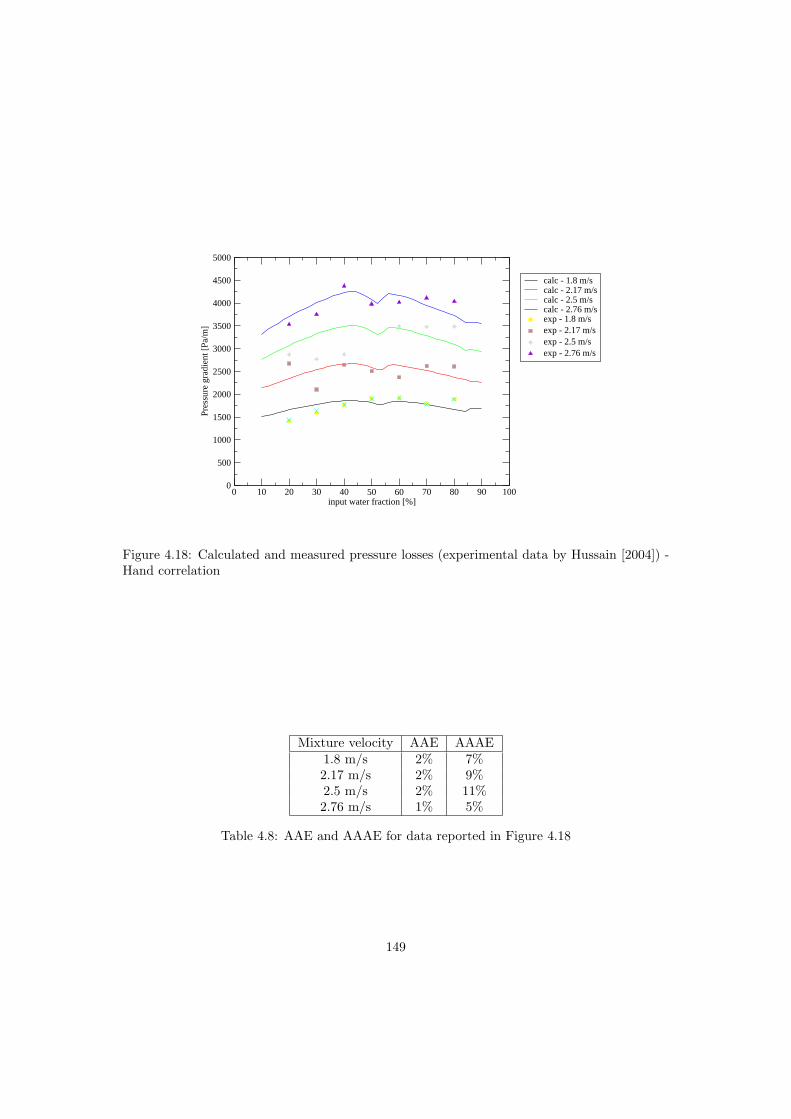
0 10 20 30 40 50 60 70 80 90 100input water fraction [%]
0
500
1000
1500
2000
2500
3000
3500
4000
4500
5000
Pres
sure
gra
dien
t [Pa
/m]
calc - 1.8 m/scalc - 2.17 m/scalc - 2.5 m/scalc - 2.76 m/sexp - 1.8 m/sexp - 2.17 m/sexp - 2.5 m/sexp - 2.76 m/s
Figure 4.18: Calculated and measured pressure losses (experimental data by Hussain [2004]) -Hand correlation
Mixture velocity AAE AAAE1.8 m/s 2% 7%2.17 m/s 2% 9%2.5 m/s 2% 11%2.76 m/s 1% 5%
Table 4.8: AAE and AAAE for data reported in Figure 4.18
149

stratified regime is obtained for intermediate values. However, both experimental data and
calculation show little effect of the flow pattern on the pressure losses. Remarkably, there is
a slight increase in the pressure gradient as the water fraction increases. This is due to the
increase in the amount of water dispersed into oil, which provide higher pressure losses than oil
dispersed into water since the mixture viscosity is higher. The difference in the viscosity of the
two fluid is, however, small and this explains the small difference in the viscosity and pressure
gradient associated with the formation of the two emulsion types.
The pressure gradients in Figure 4.18 are measured between 5.9 m and 7.77 m from the test
section inlet, where the flow was already fully developed. Other measurements were taken at
1.05, 1.55, 3.91, 3.97 and 4.91 m from inlet (Figure 4.19). Interesting observations were made
0 10 20 30 40 50 60 70 80 90input watercut [%]
0
1000
2000
3000
4000
5000
6000
7000
8000
Pres
sure
gra
dien
t [Pa
/m]
L = 1.0 mL = 1.87 mL = 2.0 mL = 3.85 mL = 5.72 mL = 6.72 m
(a) mixture velocity = 1.8 m/s
0 10 20 30 40 50 60 70 80 90input watercut [%]
0
2000
4000
6000
8000
10000
12000
14000
Pres
sure
gra
dien
t [Pa
/m]
L = 1.0 mL = 1.87 mL = 2.0 mL = 3.85 mL = 5.72 mL = 6.72 m
(b) mixture velocity = 2.76 m/s
Figure 4.19: Measured pressure gradient as a function of distance from inlet (Hussain [2004])
by Hussain, who pointed out the complex behaviour of the mixture as a function of distance.
In particular she observed that for the same mixture velocity pressure losses are higher close
to inlet and decrease further along the pipe reaching a fairly constant value. As Figure 4.19
shows, the pressure gradient close to inlet may be up to 4 times that at the end of the pipe.
This was attributed to complex mixing in the vicinity of the inlet region, which is assumed
to be responsible for the enhancement in pressure losses. The perturbation produced by the
inlet region appears to attenuate with distance and the fluids reach equilibrium conditions
towards the end of the channel. Moreover, it is possible that complex flow patterns may evolve
at pipe inlet with violent mixing, phase inversion, leading to either stratified flow or complex
150

distribution of the phases across the pipe section, which would require a more sophisticated
approach to reproduce it analytically.
Figure 4.20 presents the result obtained when the pressure losses are calculated using the
Blasius friction factor correlation.
0 10 20 30 40 50 60 70 80 90 100input water fraction [%]
0
500
1000
1500
2000
2500
3000
3500
4000
4500
5000
Pres
sure
gra
dien
t [Pa
/m]
calc - 1.8 m/scalc - 2.17 m/scalc - 2.5 m/scalc - 2.76 m/sexp - 1.8 m/sexp - 2.17 m/sexp - 2.5 m/sexp - 2.76 m/s
Figure 4.20: Pressure losses by Hussain [2004] - Blasius correlation
Mixture velocity AAE AAAE1.8 m/s -16% 16%2.17 m/s -17% 17%2.5 m/s -15% 15%2.76 m/s -19% 19%
Table 4.9: AAE and AAAE for data reported in Figure 4.20
The use of this correlation, together with the dispersion model, reproduces a trend similar
to the one obtained when using Hand’s correlation; the predictions, however, underestimate the
experimental measurements over the whole range of input water cut and for all the mixture
velocities considered (corresponding errors reported in Table 4.9). As in the previous case,
the calculation were performed applying the homogeneous model inside each layer, calculating
average densities and viscosities using Brinkman’s model, once the dispersed phase fractions are
151

calculated by the dispersion model. For input water fractions close to 50% all the predictions
show a depression corresponding to a decrease in the expected pressure gradient. The reduction
in pressure losses is due to the absence of dispersed phase inside the layers and the calculated
pressure losses correspond to the pressure losses in stratified flow. A very similar trend is
reproduced calculating the pressure losses with the Zigrang & Sylvester correlation (Figure
4.21).
0 10 20 30 40 50 60 70 80 90 100input water fraction [%]
0
500
1000
1500
2000
2500
3000
3500
4000
4500
5000
Pres
sure
gra
dien
t [Pa
/m]
calc - 1.8 m/scalc - 2.17 m/scalc - 2.5 m/scalc - 2.76 m/sexp - 1.8 m/sexp - 2.17 m/sexp - 2.5 m/sexp - 2.76 m/s
Figure 4.21: Pressure losses by Hussain [2004] - Zigrang & Sylvester correlation
Mixture velocity AAE AAAE1.8 m/s -18% 18%2.17 m/s -19% 19%2.5 m/s -16% 16%2.76 m/s -20% 20%
Table 4.10: AAE and AAAE for data reported in Figure 4.21
As in the previous case, the error between experimental data and predictions shows small
variations for the different mixture velocities examined (Table 4.10).
The same facility and the same fluids used in Hussain’s experiments were used previously in
the experiments by Soleimani [1999], but measurements of pressure losses were reported at only
152

one location (between 4.75 and 5.75 m from inlet, mid-point at 5.25). However, the development
of the pressure losses at different locations from inlet reported by Hussain (in Figure 4.19 for
example) shows that at 5.25 m from inlet fully developed flow can be expected for the mixture
velocities in Soleimani’s experiments.
Measurements of pressure gradients for pure oil and water are reported in Figure 4.22
together with the pressure gradients calculated with the various correlations for the liquid-wall
friction factor. For single-phase water flow both the Blasius and Zigrang & Sylvester correlations
0 0,5 1 1,5 2 2,5 3 3,5 4liquid velocity [m/s]
0
400
800
1200
1600
2000
2400
2800
3200
3600
4000
4400
4800
Pres
sure
gra
dien
t [Pa
/m]
experimentalHandBlasiusZigrang
(a)
0 0,5 1 1,5 2 2,5 3 3,5 4liquid velocity [m/s]
0
400
800
1200
1600
2000
2400
2800
3200
3600
4000
4400
4800
Pres
sure
gra
dien
t [Pa
/m]
experimentalHandBlasiusZigrang&Sylvester
(b)
Figure 4.22: Measured and predicted pressure losses for pure water (a) and pure oil (b)(Soleimani [1999])
provide very close results (AAAEs 16% and 17% respectively); however, Hand correlation is
closer to the experimental values (AAAE = 10%). All the correlations, however, underpredict
the single-phase oil flow pressure losses by around 15%. Data for two-phase flow were collected
by Soleimani as a function of the inlet water fraction for different mixture velocities, as shown
in Figure 2.25. Soleimani performed the experiments with smaller water cut increments than
those used by Hussain; for this reason, the peak in the pressure losses corresponding to phase
inversion was caught with more details while in the data by Hussain for high mixture velocities
the position of the narrow peak (cw ∼ 33%) is lost between two consecutive measurements (30%
and 40%). The comparison between the prediction using Hand’s correlation and experimental
data is presented in Figures 4.23 and 4.24 for low and high mixture velocities respectively while
the errors are presented in Table 4.11 for all the mixture velocities.
The expected flow patterns are the same as those in Hussain. For low mixture velocity
153

0 10 20 30 40 50 60 70 80 90 100input water cut [%]
0
200
400
600
800
1000
1200
1400
1600
1800
2000Pr
essu
re g
radi
ent [
Pa/m
]calc - 1.75 m/scalc - 1.5 m/scalc - 1.25 m/scalc - 1.0 m/sexp 1.75 m/sexp 1.5 m/sexp 1.25 m/sexp 1.0 m/s
Figure 4.23: Pressure losses by Soleimani [1999] - low mixture velocities - Hand correlation
0 10 20 30 40 50 60 70 80 90 100input water cut [%]
0
500
1000
1500
2000
2500
3000
3500
4000
4500
5000
5500
Pres
sure
gra
dien
t [Pa
/m]
calc - 3.0 m/scalc - 2.5 m/scalc - 2.0 m/sexp - 3.0 m/sexp - 2.5 m/sexp 2.1 m/s
Figure 4.24: Pressure losses by Soleimani [1999] - high mixture velocities - Hand correlation
154

Mixture velocity AAE AAAE1.0 m/s 3% 7%1.25 m/s 4% 8%1.5 m/s 11% 11%1.75 m/s 7% 7%2.1 m/s 17% 17%2.5 m/s 18% 18%3.0 m/s 28% 28%
Table 4.11: AAE and AAAE for data reported in Figures 4.23 and 4.24
there is good agreement between predictions and experimental data, as can be expected since
Soleimani’s experiments were conducted in the same facility with the same fluids as in Hussain’s
experiments. At 1.75 m/s, drag reduction starts appearing for low water cuts (< 30%) and
the magnitude of that drag reduction increases with the mixture velocity. For 2.0 m/s and
higher velocities a peak appears at about 32% inlet water cut indicating the occurrence of
phase inversion. The graphs show the model does not predict the drag reduction effect and
the peak corresponding to phase inversion is absent. While the predictions obtained from
Hand correlation match the experimental results with reasonable error at mixture velocities
up to 2.1 m/s, it overpredicts the pressure gradient for the two higher mixture velocities (2.5
m/s and 3.0 m/s). However, a comparison between the data at 2.5 m/s reported by Hussain
and by Soleimani shows a significant difference in the experimental results themselves, despite
being obtained from the same facility and with the same fluids. It has not been possible to
determine the reason behind this discrepancy (calibration of the probes, contaminants in the
fluids, changes in the temperature between the two sets of experiments).
Figures 4.25 and 4.26 compare the experimental data of Soleimani with the prediction of
the Blasius and Zigrang & Sylvester correlations respectively.
Mixture velocity Blasius Zigrang & SylvesterAAE AAAE AAE AAAE
1.0 m/s -13% 13% -15% 15%1.25 m/s -13% 13% -16% 16%1.5 m/s -9% 9% -11% 11%1.75 m/s -13% 13% -14% 14%2.1 m/s -13% 13% -14% 14%2.5 m/s -4% 7% -6% 8%3.0 m/s 1% 8% -1% 7%
Table 4.12: AAE and AAAE for data reported in Figures 4.25 and 4.26
155

0 10 20 30 40 50 60 70 80 90 100input water cut [%]
0
500
1000
1500
2000
2500
3000
3500
4000
4500
5000Pr
essu
re g
radi
ent [
Pa/m
]calc - 3.0 m/scalc - 2.5 m/scalc - 2.1 m/scalc - 1.75 m/scalc - 1.5 m/scalc - 1.25 m/scalc - 1.0 m/sexp - 3.0 m/sexp - 2.5 m/sexp 2.1 m/sexp 1.75 m/sexp 1.5 m/sexp 1.25 m/sexp 1.0 m/s
Figure 4.25: Pressure losses by Soleimani [1999] - Blasius correlation
0 10 20 30 40 50 60 70 80 90 100input water cut [%]
0
500
1000
1500
2000
2500
3000
3500
4000
4500
5000
Pres
sure
gra
dien
t [Pa
/m]
calc - 3.0 m/scalc - 2.5 m/scalc - 2.1 m/scalc - 1.75 m/scalc - 1.5 m/scalc - 1.25 m/scalc - 1.0 m/sexp - 3.0 m/sexp - 2.5 m/sexp 2.1 m/sexp 1.75 m/sexp 1.5 m/sexp 1.25 m/sexp 1.0 m/s
Figure 4.26: Pressure losses by Soleimani [1999] - Zigrang & Sylvester correlation
156

As for the previous set of data, at low mixture velocities all the correlations examined
provide similar results: all are in good agreement with the experimental data. Contrary to
the predictions with Hand correlation (Figure 4.23), pressure loss at low mixture velocities in
Figures 4.25 and 4.26 underestimate the experimental values. The prediction of lower pressure
gradients is confirmed at high mixture velocities, where Blasius and Zigrang & Sylvester predict
pressure losses closer to the experimental values than Hand correlation. As in the case of the
Hand correlation, they do not allow for drag reduction and the peak corresponding to phase
inversion is not reproduced.
In Figure 4.27 the pressure gradients for pure oil and pure water measured by Elseth [2001]
are compared against predictions. Again, the Blasius and Zigrang & Sylvester correlations give
very similar results but, contrary to the Soleimani data, they are closer to the experimental data
than Hand’s correlation. Figures 4.28, 4.29 and 4.30 compare the calculated pressure losses for
0 0,5 1 1,5 2 2,5 3 3,5 4liquid velocity [m/s]
0
200
400
600
800
1000
1200
1400
1600
1800
2000
2200
2400
Pres
sure
gra
dien
t [Pa
/m]
experimentalHandBlasiusZigrang
(a)
0 0,5 1 1,5 2 2,5 3 3,5 4liquid velocity [m/s]
0
200
400
600
800
1000
1200
1400
1600
1800
2000
Pres
sure
gra
dien
t [Pa
/m]
experimentalHandBlasiusZigrang
(b)
Figure 4.27: Measured and predicted pressure losses for pure water (a) and pure oil (b) (Elseth[2001])
the experiments of Elseth [2001] with the experimental data.
Despite the physical properties of the oil used by Elseth being similar to those of the oil
used by Soleimani and Hussain (compare Tables 4.2 and 4.6), Elseth reports no peak in the
pressure losses associated with phase inversion. However, Elseth’s measurements are not as
detailed as those of Soleimani and for high mixture velocities, few points were collected by
Elseth around the water cut at which Soleimani reported phase inversion. The comparisons
with the experimental data by Elseth confirm that all the correlations used for the pressure loss
157

0 10 20 30 40 50 60 70 80 90 100input water cut [%]
0
200
400
600
800
1000
1200
1400
1600
1800
2000Pr
essu
re g
radi
ent [
Pa/m
]calc - 1.34 m/scalc - 1.5 m/scalc - 1.67 m/scalc - 2.0 m/scalc - 2.5 m/scalc - 3.0 m/sexp - 1.34 m/sexp - 1.5 m/sexp - 1.67 m/sexp - 2.0 m/sexp - 2.5 m/sexp - 3.0 m/s
Figure 4.28: Measured and predicted pressure losses with Hand correlation (experimental databy Elseth [2001])
0 10 20 30 40 50 60 70 80 90 100input water cut [%]
0
200
400
600
800
1000
1200
1400
1600
1800
2000
Pres
sure
gra
dien
t [Pa
/m]
calc - 1.34 m/scalc - 1.5 m/scalc - 1.67 m/scalc - 2.0 m/scalc - 2.5 m/scalc - 3.0 m/sexp - 1.34 m/sexp - 1.5 m/sexp - 1.67 m/sexp - 2.0 m/sexp - 2.5 m/sexp - 3.0 m/s
Figure 4.29: Measured and predicted pressure losses with Blasius correlation (experimentaldata by Elseth [2001])
158

0 10 20 30 40 50 60 70 80 90 100input water cut [%]
0
200
400
600
800
1000
1200
1400
1600
1800
2000
Pres
sure
gra
dien
t [Pa
/m]
calc - 1.34 m/scalc - 1.5 m/scalc - 1.67 m/scalc - 2.0 m/scalc - 2.5 m/scalc - 3.0 m/sexp - 1.34 m/sexp - 1.5 m/sexp - 1.67 m/sexp - 2.0 m/sexp - 2.5 m/sexp - 3.0 m/s
Figure 4.30: Measured and predicted pressure losses with Zigrang & Sylvester correlation (ex-perimental data by Elseth [2001])
evaluation overpredict the experimental results for high mixture velocities while they all show
good agreement at low mixture velocities (Table 4.13).
Mixture velocity Hand Blasius Zigrang & SylvesterAAE AAAE AAE AAAE AAE AAAE
1.34 m/s 15% 17% -4% 8% -4% 9%1.5 m/s 25% 25% 6% 11% 4% 9%1.67 m/s 26% 26% 5% 10% 5% 10%2.0 m/s 36% 36% 14% 14% 14% 14%2.5 m/s 50% 50% 24% 25% 24% 25%3.0 m/s 56% 56% 27% 27% 27% 27%
Table 4.13: AAE and AAAE for pressure losses measured by Elseth [2001]
Despite the absolute values of the pressure losses depend on the fluid properties and the pipe
characteristics the calculated pressure losses for Soleimani, Hussain and Elseth’s experiments
at high mixture velocities reproduce similar trends with the lower pressure losses calculated
for single phase flow and no drag reduction when dispersion of the phases occurs, as instead
happens in the experimental measurements.
The results shown in the previous comparison are further confirmed by the experimental
159

measurements of oil-water pressure drop performed by Lovick [2004] in a horizontal test section
using the fluids and the geometry in Table 4.1.
Figure 4.31 shows that the pressure losses for pure water and pure oil are well predicted by
all the correlations, with AAAEs ranging from 7% (Hand) to 11% (Blasius) for pure oil and
from 5% (Blasius) to 9% (Hand) for pure water.
0 0,5 1 1,5 2 2,5 3 3,5 4liquid velocity [m/s]
0
400
800
1200
1600
2000
2400
2800
3200
3600
4000
Pres
sure
gra
dien
t [Pa
/m]
experimentalHandBlasiusZigrang&Sylvester
(a)
0 0,5 1 1,5 2 2,5 3 3,5 4liquid velocity [m/s]
0
400
800
1200
1600
2000
2400
2800
3200
3600
4000
Pres
sure
gra
dien
t [Pa
/m]
experimentalHandBlasiusZigrang&Sylvester
(b)
Figure 4.31: Measured and predicted pressure losses for pure water (a) and pure oil (b) (Lovick[2004])
Figures 4.32, 4.33, and 4.34 show the comparison with the experimental data by Lovick
[2004] for different mixture velocities as a function of the inlet water fraction. The errors
reported in Table 4.14 indicate that all the correlations tend to overpredict the experimental
data at all mixture velocities. Contrary to the previous sets of data, the discrepancies do not
seem to increase at higher mixture velocities.
Mixture velocity Hand Blasius Zigrang & SylvesterAAE AAAE AAE AAAE AAE AAAE
0.8 m/s 57% 57% 50% 50% 55% 55%1.0 m/s 54% 54% 34% 34% 34% 34%1.5 m/s 55% 55% 51% 51% 49% 49%2.0 m/s 47% 48% 41% 54% 39% 51%2.5 m/s 58% 58% 51% 56% 48% 53%3.0 m/s 47% 47% 38% 53% 36% 49%3.5 m/s 32% 32% 20% 24% 12% 17%
Table 4.14: AAE and AAAE for pressure losses measured by Lovick [2004]
160

0 10 20 30 40 50 60 70 80 90 100input water fraction [%]
0
500
1000
1500
2000
2500
3000
3500
4000
4500
5000Pr
essu
re g
radi
ent [
m/s
]calc - 0.8 m/scalc - 1.0 m/scalc - 1.5 m/scalc - 2.0 m/scalc - 2.5 m/scalc - 3.0 m/scalc - 3.5 m/sexp - 0.8 m/sexp - 1.0 m/sexp - 1.5 m/sexp - 2.0 m/sexp - 2.5 m/sexp - 3.0 m/sexp - 3.5 m/s
Figure 4.32: Measured and predicted pressure losses - Hand correlation (Lovick [2004])
0 10 20 30 40 50 60 70 80 90 100input water fraction [%]
0
500
1000
1500
2000
2500
3000
3500
4000
4500
5000
Pres
sure
gra
dien
t [m
/s]
calc - 0.8 m/scalc - 1.0 m/scalc - 1.5 m/scalc - 2.0 m/scalc - 2.5 m/scalc - 3.0 m/scalc - 3.5 m/sexp - 0.8 m/sexp - 1.0 m/sexp - 1.5 m/sexp - 2.0 m/sexp - 2.5 m/sexp - 3.0 m/sexp - 3.5 m/s
Figure 4.33: Measured and predicted pressure losses - Blasius correlation (Lovick [2004])
161

0 10 20 30 40 50 60 70 80 90 100input water fraction [%]
0
500
1000
1500
2000
2500
3000
3500
4000
4500
5000
Pres
sure
gra
dien
t [m
/s]
calc - 0.8 m/scalc - 1.0 m/scalc - 1.5 m/scalc - 2.0 m/scalc - 2.5 m/scalc - 3.0 m/scalc - 3.5 m/sexp - 0.8 m/sexp - 1.0 m/sexp - 1.5 m/sexp - 2.0 m/sexp - 2.5 m/sexp - 3.0 m/sexp - 3.5 m/s
Figure 4.34: Measured and predicted pressure losses - Zigrang & Sylvester correlation (Lovick[2004])
4.4.1 Turbulence reduction due to dispersion of the phases - Effects
on pressure losses
A feature in common to the comparisons against both the data of Soleimani and of Elseth is
that the calculated pressure drops at high mixture velocity are overpredicted. Moreover, high
mixture velocities show drag reduction effects and the experimental pressure losses for two-phase
flow are often below the measured pressure losses for single-phase flow. Drag reduction was
studied in the experimental work by Pal [1993], who attributed it to coalescence and breakup
of the dispersed phase droplets. In particular, coalescence may lead to the formation of big
drops that would somehow inhibit the continuous phase turbulence; moreover, breakup and
coalescence would also act as energy sinks for the turbulent energy of the continuous phase.
Experimental evidence provided by Pal showed that water-in-oil emulsions exhibited higher
drag reduction than oil-in-water dispersions and laminar flow could persist at Reynolds number
up to 4000 (see Figure 4.35).
The predictions of the two-fluid model closed by the present dispersion model do not ac-
162

Figure 4.35: Friction factors for unstable oil-in-water and water-in-oil dispersions (Pal [1993])
163

count for drag reduction effects. With the hypothesis of fully dispersed flow and homogeneous
distribution across the pipe section of the dispersed phase, the pressure gradient in the pipe
can be obtained from the simple expression
d p
dx= −1
2ρMfMu2
M − ρMg sin γ, (4.6)
where the mixture density is given by ρM = cwρw + (1− cw) ρo. Fully dispersed flow and
homogeneous dispersion are limited to high mixture velocities; as an example, Figure 4.36
compares the experimental pressure losses reported by Soleimani at 3.0 m/s with the predictions
of Equation (4.6) coupled with the friction factors correlations by Blasius, Hand and Zigrang
& Sylvester (Equations (3.11), (3.16) and (3.12) respectively) All the correlations give similar
0 10 20 30 40 50 60 70 80 90 100input water cut [%]
0
1000
2000
3000
4000
5000
6000
7000
Pres
sure
gra
dien
t [Pa
/m]
BlasiusHandZigrang & Sylvesterexperimental
Figure 4.36: Soleimani’s data against correlation available and homogeneous model - mixturevelocity = 3.0 m/s
predictions: starting from pure oil and increasing the water percentage the predicted pressure
gradient increases up to the point of phase inversion, which for this calculation was deduced
from the experimental data. A sudden jump corresponds to the point of phase inversion;
subsequently, the pressure loss decreases monotonically for increasing water fraction.
164
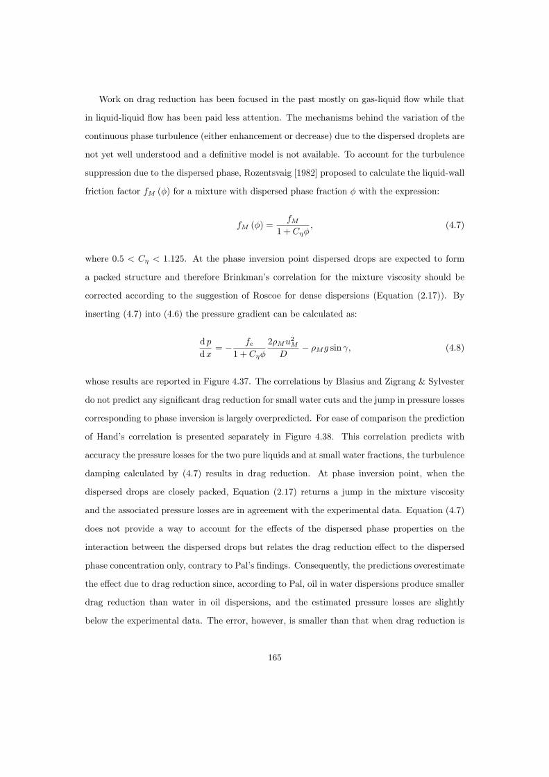
Work on drag reduction has been focused in the past mostly on gas-liquid flow while that
in liquid-liquid flow has been paid less attention. The mechanisms behind the variation of the
continuous phase turbulence (either enhancement or decrease) due to the dispersed droplets are
not yet well understood and a definitive model is not available. To account for the turbulence
suppression due to the dispersed phase, Rozentsvaig [1982] proposed to calculate the liquid-wall
friction factor fM (φ) for a mixture with dispersed phase fraction φ with the expression:
fM (φ) =fM
1 + Cηφ, (4.7)
where 0.5 < Cη < 1.125. At the phase inversion point dispersed drops are expected to form
a packed structure and therefore Brinkman’s correlation for the mixture viscosity should be
corrected according to the suggestion of Roscoe for dense dispersions (Equation (2.17)). By
inserting (4.7) into (4.6) the pressure gradient can be calculated as:
d p
dx= − fe
1 + Cηφ
2ρMu2M
D− ρMg sin γ, (4.8)
whose results are reported in Figure 4.37. The correlations by Blasius and Zigrang & Sylvester
do not predict any significant drag reduction for small water cuts and the jump in pressure losses
corresponding to phase inversion is largely overpredicted. For ease of comparison the prediction
of Hand’s correlation is presented separately in Figure 4.38. This correlation predicts with
accuracy the pressure losses for the two pure liquids and at small water fractions, the turbulence
damping calculated by (4.7) results in drag reduction. At phase inversion point, when the
dispersed drops are closely packed, Equation (2.17) returns a jump in the mixture viscosity
and the associated pressure losses are in agreement with the experimental data. Equation (4.7)
does not provide a way to account for the effects of the dispersed phase properties on the
interaction between the dispersed drops but relates the drag reduction effect to the dispersed
phase concentration only, contrary to Pal’s findings. Consequently, the predictions overestimate
the effect due to drag reduction since, according to Pal, oil in water dispersions produce smaller
drag reduction than water in oil dispersions, and the estimated pressure losses are slightly
below the experimental data. The error, however, is smaller than that when drag reduction is
165
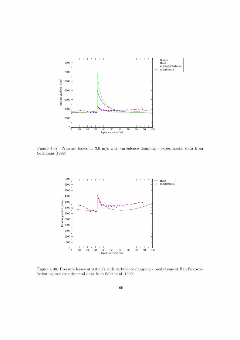
0 10 20 30 40 50 60 70 80 90 100input water cut [%]
0
2000
4000
6000
8000
10000
12000
14000Pr
essu
re g
radi
ent [
Pa/m
]BlasiusHandZigrang & Sylvesterexperimental
Figure 4.37: Pressure losses at 3.0 m/s with turbulence damping - experimental data fromSoleimani [1999]
0 10 20 30 40 50 60 70 80 90 100input water cut [%]
0
500
1000
1500
2000
2500
3000
3500
4000
4500
5000
5500
6000
Pres
sure
gra
dien
t [Pa
/m]
Handexperimental
Figure 4.38: Pressure losses at 3.0 m/s with turbulence damping - predictions of Hand’s corre-lation against experimental data from Soleimani [1999]
166

unaccounted for and the AAAE is 5% for the oil continuous region (left of the phase inversion
point) and 7% for the water continuous region (right of the phase inversion point). Figure 4.39
shows the pressure losses calculated applying the mixing model together with the turbulence
reduction model proposed by Rozentsvaig [1982] for all mixture velocities covered in Soleimani’s
work. The results are obtained for Cη = 1.0 in Equation (4.7), Brinkman’s model for mixture
viscosity and Hand’s correlation for liquid-wall friction factor.
0 10 20 30 40 50 60 70 80 90 100input water cut [%]
0
500
1000
1500
2000
2500
3000
3500
4000
4500
5000
Pres
sure
gra
dien
t [Pa
/m]
exp - 3.0 m/sexp - 2.5 m/sexp 2.1 m/sexp 1.75 m/sexp 1.5 m/sexp 1.25 m/sexp 1.0 m/scalc - 1.0 m/scalc - 1.25 m/scalc - 1.5 m/scalc - 1.75 m/scalc - 2.1 m/scalc - 2.5 m/scalc - 3.0 m/s
Figure 4.39: Pressure gradient calculated with turbulence damping according to Rozentsvaig[1982] and Hand correlation (experimental data by Soleimani [1999])
Mixture velocity AAE AAAE AAAE without drag reduction1.0 m/s -14% 14% 4%1.25 m/s -17% 17% 4%1.5 m/s -14% 14% 10%1.75 m/s -17% 17% 7%2.1 m/s -12% 12% 5%2.5 m/s -13% 13% 18%3.0 m/s -7% 7% 30%
Table 4.15: Errors for pressure losses calculated with turbulence reduction (Figure 4.39). Com-parison with the errors presented without turbulence reduction (Figures 4.23 and 4.24)
It is interesting to compare the errors reported in Table 4.15 for the predictions obtained with
167

and without the drag reduction term. For mixture velocities up to 2.1 m/s the predicted pressure
losses without drag reduction were slightly higher then the measured pressure losses, with errors
ranging from 4% to 10%. The introduction of the drag reduction term shifted the predicted
pressure losses towards lower values, yielding the underprediction of the experimental losses
and larger errors than those affecting the calculation without drag reduction. The change from
average overprediction to underprediction can be observed even at higher mixture velocities but
the average error between predictions and experimental values becomes smaller. Equation (4.7)
does not provide any indication whether the effects of the dispersed phase on the continuous
phase turbulence depend on the Reynolds number; therefore, the correlation was applied both
at high and at low mixture velocities. The results of the calculations, however, seem to suggest
that the use of drag reduction at low mixture velocities is perhaps inappropriate. However, the
data were not provided with error bars and it is not possible to determine if either prediction
(with or without turbulence reduction) falls outside the error range; in any event, the error
relative to the experimental data remains small over the whole range of input water cuts.
At high mixture velocities and low water cuts the predictions of the model are close to the
experimental data: the drag reduction effect provides decreasing pressure losses as the water
cut increases up to ∼ 18%. The peak at phase inversion is not predicted by the model; neither
the phase inversion criteria proposed by Decarre and Fabre nor those derived by Brauner and
Ullmann predict phase inversion point that is observed to be at 32% water cut (the predicted
phase inversion points are 51% and 49% water cut respectively). However, it is possible that the
experimental phase inversion point is affected by secondary dispersion, which is not accounted
for by the present dispersion model. For water cuts above 40% both experimental measurements
and predicted pressure losses increase as the oil percentage reduces to small amounts.
There is a small peak in the calculated pressure losses corresponding to the range of water
cuts 0.55−0.6 which results from the absence of dispersion predicted in that region. As indicated
in the discussion on flow pattern, small dispersed phase fractions are predicted by the dispersion
model when the slip velocity between the continuous phases in the two layers approaches zero,
independently from the mixture velocity. The peak is due to the lack of dispersion between the
phases and the consequent absence of drag reduction. The peak, therefore, gives pressure losses
for stratified flow of pure liquids. When drag reduction is not accounted for, the stratification
168

of the fluids corresponds to a decrease in pressure loss since the viscosity in each layer would
not be increased by the presence of a dispersed phase.
When the turbulence reduction term is used together with the Blasius correlation the cal-
culated pressure losses are as shown in Figure 4.40.
0 10 20 30 40 50 60 70 80 90 100input water cut [%]
0
500
1000
1500
2000
2500
3000
3500
4000
4500
5000
Pres
sure
gra
dien
t [Pa
/m]
calc - 3.0 m/scalc - 2.5 m/scalc - 2.0 m/scalc - 1.75 m/scalc - 1.5 m/scalc - 1.25 m/scalc - 1.0 m/sexp - 3.0 m/sexp - 2.5 m/sexp 2.1 m/sexp 1.75 m/sexp 1.5 m/sexp 1.25 m/sexp 1.0 m/s
Figure 4.40: Pressure gradient calculated with turbulence damping according to Rozentsvaig[1982] and Blasius correlation (experimental data by Soleimani [1999])
Mixture velocity AAE AAAE AAAE without drag reduction1.0 m/s -17% 17% 1%1.25 m/s -21% 21% 13%1.5 m/s -19% 19% 13%1.75 m/s -24% 24% 13%2.1 m/s -19% 19% 13%2.5 m/s -21% 21% 7%3.0 m/s -17% 17% 8%
Table 4.16: Errors for pressure losses calculated with turbulence reduction (Figure 4.40). Com-parison with the errors presented without turbulence reduction (Figure 4.25)
The predicted results differ widely from those reported in Figure 4.39. Since the use of
the Blasius correlation without the turbulence suppression correction provides pressure losses
already close to the experimental results (Figure 4.25), the addition of the turbulence reduction
169

term leads to underprediction of the experimental results (Table 4.16) with overall errors larger
than without turbulence reduction. The addition of this term when using Blasius correlation
for the liquid-wall friction factor does not result in drag reduction; moreover, a striking feature
of the calculated pressure losses is that they are almost constant for each mixture velocity. This
result is due to the equilibrium between turbulence reduction and increasing viscosity of the
mixture due to dispersion.
Figure 4.41 shows a comparison between the experimental pressure losses obtained by Elseth
[2001] and the pressure gradient calculated using both the Hand and Blasius correlations with
the turbulence reduction model of Rozentsvaig. The predicted pressure losses well match the
Mixture velocity Hand correlation Blasius correlationAAAE withd. r.
AAAE withoutd. r.
AAAE withd. r.
AAAE withoutd. r.
1.0 m/s 11% 17% 10% 8%1.25 m/s 14% 25% 6% 11%1.5 m/s 13% 26% 7% 10%1.75 m/s 21% 35% 7% 14%2.1 m/s 27% 50% 11% 25%2.5 m/s 27% 56% 8% 27%
Table 4.17: Errors for pressure losses calculated with turbulence reduction (Figure 4.41). Com-parison with the errors presented without turbulence reduction (Figures 4.28 and 4.29). d. r.= drag reduction correlation.
experimental data for low mixture velocities, where both correlations provide results close to the
measurements and in better agreement than without drag reduction. An improvement is also
observed at high mixture velocities, with the Blasius correlation giving the best comparison
with the experimental values. Hand’s correlation manifests the tendency to overpredict the
experimental results and this tendency becomes stronger as the mixture velocity increases
despite the drag reduction effects accounted for by Rozentsvaig’s correction. As in the case
of Soleimani’s pressure losses, the relative peak at intermediate water cuts is due to modest
dispersion of the phases for those water cuts. This peak is diminished when using the Blasius
correlation which, in turn, predicts a flat profile for the pressure losses even at high mixture
velocities when, instead, the experimental pressure gradient constantly increases for water cut
higher than 35%.
An interesting explanation for the drag reduction mechanism was proposed by Pal [2007]
170

0 10 20 30 40 50 60 70 80 90 100input water cut [%]
0
200
400
600
800
1000
1200
1400
1600
1800
2000Pr
essu
re g
radi
ent [
Pa/m
]
calc - 1.34 m/scalc - 1.5 m/scalc - 1.67 m/scalc - 2.0 m/scalc - 2.5 m/scalc - 3.0 m/sexp - 1.34 m/sexp - 1.5 m/sexp - 1.67 m/sexp - 2.0 m/sexp - 2.5 m/sexp - 3.0 m/s
(a) Pressure losses calculated with Hand’s correlation
0 10 20 30 40 50 60 70 80 90 100input water cut [%]
0
200
400
600
800
1000
1200
1400
1600
1800
2000
Pres
sure
gra
dien
t [Pa
/m]
calc - 1.34 m/scalc - 1.5 m/scalc - 1.67 m/scalc - 2.0 m/scalc - 2.5 m/scalc - 3.0 m/sexp - 1.34 m/sexp - 1.5 m/sexp - 1.67 m/sexp - 2.0 m/sexp - 2.5 m/sexp - 3.0 m/s
(b) Pressure losses calculated with Blasius’ correlation
Figure 4.41: Pressure losses (Elseth [2001])
171

who related it to the reduction in the effective viscosity of the dispersion when the flow regime
changes from laminar to turbulent. The starting point of Pal’s study is the theoretical model
for the relative viscosity µr of concentrated dispersions published by him (Pal [2003]):
µr
[CM − CP + 32µr
CM − CP + 32
]CN−1.25 [CM + CP − 32
CM + CP − 32µr
]CN+1.25
= exp
2.5φ
1− φ
φm
, (4.9)
where φm is the maximum packing volume fraction of droplets and
CM =
√64
N2Ca
+ 1225λ2µ + 1232
λµ
NCa, (4.10)
CP =8
NCa− 3λµ, (4.11)
CN =(22/NCa) + 43.75λµ
CM. (4.12)
Pal studied the behaviour of the mixture viscosity at different capillary number NCa when the
viscosity ratio λµ, defined as the ratio between the dispersed and continuous phase viscosities, is
higher or smaller than 1. He concluded that the laminar and turbulent pipe flow of dispersions
can be treated with the approximations of low capillary number flow and high capillary number
flow respectively. With these hypotheses, Equation (4.9) reduces to:
µr,o
[2µr,∞ + 5λµ
2 + 5λµ
]3/2
= exp
2.5φ
1− φ
φm
(4.13)
for low capillary numbers and to:
µr,∞
[λµ − µr,∞
λµ − 1
]−2.5
= exp
2.5φ
1− φ
φm
, (4.14)
for high capillary numbers. The quantities µr,o and µr,∞ are the limiting relative viscosities at
low and high capillary number respectively. The results of Equations (4.13) and (4.14) were
plotted by Pal for different maximum packing fractions as a function of the volume fraction of
172

dispersed phase as in Figure 4.42.
(a) (b)
Figure 4.42: Relative viscosity for emulsions with λµ < 1 (a) and λµ > 1 (b) (Pal [2007])
The value of φm depends on the drop size distribution and does not to have to be the
same for oil-in-water and water-in-oil emulsions. The case of λµ < 1.0 typically corresponds
to water in oil emulsions while λµ > 1.0 is the case of oil dispersed in water. The theoretical
results in Figure 4.42(a) show that at high capillary numbers and when water is the dispersed
phase (λµ < 1.0), an increase in the dispersed water phase fraction yields a decrease in the
effective viscosity of the mixture. At low capillary numbers, on the contrary, the mixture
viscosity increases for increasing dispersed phase fraction. Figure 4.42(b), instead, shows that
for oil-in-water emulsions the predicted mixture viscosity would increase for increasing dispersed
phase fractions regardless of the capillary number. The predictions of Equation (4.9) for the
fluids used by Soleimani [1999] are reported in Figure 4.43, which confirms the trends reported
in Pal’s work. The reduction in the relative viscosity for water-in-oil emulsions in Figure
4.43(a) is smaller than that reported in Pal’s work (Figure 4.42(a)) due to the relatively small
difference in the viscosities of the fluids used by Soleimani compared to the viscosity ratio in
Pal’s calculations.
From observation of experimental data, Pal suggests that the turbulent pipe flow of dis-
persions can be treated as high capillary number flow, thus employing Equation (4.14) for the
calculation of mixture relative viscosity. The comparison between the prediction of the model
by Pal and the experimental results of Soleimani for uM = 3.0 m/s are presented in Figure
4.44.
The dispersed phase fraction (either water or oil) was supposed to be homogeneously dis-
173

(a)
(b)
Figure 4.43: Relative viscosity for water-in-oil (a) and oil-in-water (b) emulsions from Equations(4.13) and (4.14) - Fluids properties as in Soleimani [1999]
174

0 10 20 30 40 50 60 70 80 90 100input water cut [%]
0
300
600
900
1200
1500
1800
2100
2400
2700
3000
3300
3600
3900
4200
4500
Pres
sure
gra
dien
t [Pa
/m]
BlasiusHandZigrang & SylvesterPrandtlexperimental
Figure 4.44: Pressure gradient measured by Soleimani compared with the prediction of Equation(4.14) with φm = 0.5 for water in oil dispersions and φm = 0.74 for oil in water dispersions.
175

tributed across the pipe section and the transition from oil continuous to water continuous was
assumed to occur at 32% water cut. Different values for φm were applied in the case of water
in oil (φm = 0.5) and oil in water (φm = 0.74) emulsions in order to obtain predictions close to
the experimental data; the flow was assumed to be turbulent and Equation (4.14) was therefore
used to evaluate the mixture viscosity.
For water in oil dispersions (λµ < 1) all the correlations tested predict almost constant
pressure losses; only the Hand correlation show a slightly increasing trend. After phase inversion
and the transition from oil continuous to water continuous (λµ > 1) the experimental data show
an increase in the pressure loss after the sharp decrease immediately after phase inversion. This
trend is reproduced by the Hand correlation, with predicted values close to the experimental
values. The other correlations, instead, manifest a weaker dependence on the water fraction,
with a slightly decreasing trend. It can be observed in Figure 4.44 that there is a gap between
the two branches of each curve and not all the possible input water fractions are covered by
the predictions. A limit of Equation (4.14) is that the existence of the solution for a given φ
depends on the values of λµ and φm; with the values of φm used in the calculations a solution
could not be found when 32.0% < φ < 39.2%. Different choices of φm affect both the amplitude
of this gap and, obviously, the value of the mixture viscosity in the region of dispersed phase
fraction where a solution of Equation (4.14) exists.
4.5 Results obtained with the de Bertodano et al. [1998]
correlation
All the results previously presented in the chapter are obtained applying the correlation
of Chesters and Issa (Equation (3.53)) for the entrainment rates of water into oil and oil into
water. In Appendix C the predictions of the Lopez de Bertodano et al. correlation are presented
for a selection of the experimental data by Al-Wahaibi [2006], Elseth [2001], Soleimani [1999],
Hussain [2004] and Lovick [2004]. The analysis of the dispersed phase fractions (Figures C-1 to
C-11) highlights two problems encountered in the use of this correlation. Firstly it is affected
by the same lack of entrainment at small slip velocities exhibited by the Chesters and Issa
176
correlation. The lack of dispersion between the phases is also responsible for the trend of the
pressure losses results, with peaks corresponding to the regions of formation of emulsions and
lower values at intermediate water cuts where little dispersion is predicted. The correlation
of Lopez de Bertodano et al. also suffers the inaccuracy in the choice of the critical Reynolds
number for the initiation of entrainment. The values of the critical Reynolds number (7000
for the formation of water drops and 3300 for the formation of oil drops) used to generate the
results presented in the appendix provide good predictions of the data of Elseth [2001], but
they underpredict the other results obtained at low mixture velocities. Results might improve
with a finer tuning of the adjustable parameters of the correlation against detailed sets of data
collected at the smallest velocities when entrainment begins. The pressure losses reported in
Figures C-12 to C-20 have characteristics similar to those presented using the Chesters and Issa
correlation. The trend is dictated by the viscosity of the emulsions resulting from the formation
of dispersed drops and, therefore, high dispersed fractions result in high mixture viscosity and
high pressure losses. As with the other correlation, the effects of drag reduction can only be
obtained by introducing turbulence dumping factors.
4.6 Discussion
The proposed model for two-phase liquid-liquid flow in pipe was validated and comparisons
against experimental data were presented in this chapter. Conclusions from the comparisons
can be drawn for dispersed phase fraction, pressure losses and flow regimes predicted by the
model.
• Dispersed phase fractions
The two proposed correlations for the entrainment rate are related to the slip between the
phases since it is supposed that the shear stress between the phases produces interfacial waves
and filaments of one phase protruding into the other, from which drops are detached. The
comparison with experimental data show good agreement. In most of the cases, the model
reproduces the dispersed phase fractions that are obtainable from the equilibrium between
entrainment and deposition between the layers, for different phase ratios and mixture velocities.
177

Discrepancies may be noted at very low mixture velocities when turbulence at low Reynolds
number can be expected. Both entrainment correlations are derived on the assumption of
highly turbulent flow; it is not surprising, then, that when the conditions for laminar flow are
approached the predictions of the model do not match the experimental data. The transition
from partially dispersed flow to fully dispersed flow is signalled by phase inversion, which occurs
at cw ∼ 32% in the experimental data of Hussain, Soleimani and Elseth. The model, however,
calculates the critical oil fraction for phase inversion with the Decarre and Fabre criteria which,
for turbulent flow before and after phase inversion, do not predict a critical oil fraction much
different from 50% when the fluids density and viscosity do not differ largely. Similar results
are predicted when using the Brauner and Ullmann criteria for phase inversion.
• Pressure loss
The main factor connected with the evaluation of the pressure losses is the choice of the empirical
correlation required for the friction factors between liquid and internal pipe wall and for the
interfacial friction. This choice also influences the friction velocity, a quantity that is used in
the calculation of the entrainment and deposition rates. The choice of the wall-liquid friction
factor correlation, therefore, affects not only the pressure loss calculation but the dispersed
phase fraction evaluation and the flow pattern as well.
Three correlations were tested: Hand, Blasius and Zigrang & Sylvester. The use of Hand’s
correlation leads to overprediction in the pressure losses while the Blasius correlation and the
Zigrang & Sylvester correlations yield smaller errors overall. All the correlations examined pro-
vide good results at low and intermediate mixture velocities, when stratified flow or partially
dispersed flow is expected and predicted. It must be kept in mind that the numerical results
are obtained supposing that the emulsions formed in each layer behave as single fluids; this
hypothesis is not always verified (see, for example, Baron et al. [1953]). At high mixture veloci-
ties all the correlations adopted show significant discrepancy when compared with experimental
data, and drag reduction, shown by the experiments, is not reproduced computationally. The
predicted pressure loss is dictated by the viscosity of the mixture formed after dispersion of
the phases, which, according to Brinkman’s model, is always higher than the continuous phase
viscosity. A simple model (Rozentsvaig [1982]) was tested in the present work to show that
178

accounting for drag reduction effects due to dispersion of the phases results in slightly improved
prediction. Small drag reduction effects were obtained in the predicted pressure losses at high
mixture velocity; the experimental drag reduction, however, may be due not only to turbulence
reduction but also to other factors, such as the preferential wetting of the pipe wall by the less
viscous phase. A quick overview of the model by Pal [2007] for the calculation of the mixture
viscosity was presented. The model offers the advantage of making a distinction between lam-
inar and turbulent flow and in the latter case can predict a different behaviour of oil-in-water
and water-in-oil mixtures for varying dispersed phase concentration. Numerical weaknesses of
the model were highlighted. The difficulties encountered in the calculation of the critical oil
fraction for phase inversion affect the prediction of pressure losses as well, since the peak in
the pressure gradient corresponding to phase inversion is not reproduced by the calculation.
The use of the Blasius and Zigrang & Sylvester correlations give pressure losses at high mixture
velocities close to the average of the experimental values, although the predictions do not repro-
duce the details of the experimental trends. This might indicate that the model captures only
the average behaviour of the phases in the pipe since it is based on a simplification of the spatial
phase distribution. Increasing the complexity of the model to account for the distribution of
the phases (for example, introducing the calculation of the interface curvature) together with
improvements in the determination of the phase inversion point and accounting for secondary
dispersion might improve the overall prediction at the cost of increased model complexity.
• Flow patterns
Experimental flow patterns were regrouped to match the flow patterns accounted for by the
model (stratified flow, partially dispersed flow and fully dispersed flow). The model showed
good overall agreement with the experimental flow maps, especially at low and intermediate
mixture velocities over most of the experimental water cuts. The reasons for the persistence of
stratified flow at intermediate water cuts and high mixture velocities have been discussed and
solutions are left for future work.
179

180
Chapter 5
Three-phase oil/water/gas flow
5.1 Preamble
A model was proposed in chapter 3 for the computational simulation of liquid/liquid flow in
pipelines. The model is extended in this chapter to three-phase oil/water/gas flow within the
framework of the existing research code TRIOMPH for the simulation of two and three-phase
slug flow.
The TRIOMPH code solves the equations of the two-fluid model in an Eulerian frame;
when solving the equations of the model, random perturbations within the solution process
generate gas-liquid interfacial disturbances that may grow becoming waves and slugs (slug
capturing technique). The TRIOMPH code has been extensively validated for two-phase gas-
liquid flow (Issa and Abrishami [1986], Rippiner [1998], Issa and Woodburn [1998], Issa and
Kempf [2003]) and the slug capturing technique has proved capable of simulating the formation
and the dynamic development of slugs inside horizontal and inclined pipes.
Bonizzi and Issa [2003] extended the application of the two-fluid model to the simulation
of three-phase gas/liquid/liquid flow using the TRIOMPH code. The model proposed by the
authors is able to account for two flow patterns only in the liquid phases, namely stratified
and fully dispersed flow, and the transition from one flow pattern to the other occurs abruptly,
without accounting properly for dispersion and segregation transition situations. The addition
181

of the present dispersion model provides a tool to predict the distribution of the phases inside
the liquid mass, both in the film between two slugs and inside the slug body, predicting the
kind of emulsions formed inside the liquid.
Section 5.2 describes the framework used in TRIOMPH for the simulation of three-phase
flow using the two-fluid model and illustrates the equations solved by the code together with
the closure models required. The implementation of the equations of the dispersion model is
discussed in section 5.3 and the results of the model are then compared against experimental
data and discussed in section 5.4. Conclusions are drawn at the end of the chapter (section
5.5).
5.2 Equations for three-phase gas/liquid/liquid flow
The aim of this work is the simulation of the pipeline flow of two liquid phases and one
gas phase. The most obvious choice is the solution of the continuity and momentum equations
for each of the phases as already done, for example, in the approach proposed by Taitel et al.
[1995]. In the present work, however, the approach adopted by Bonizzi and Issa [2003] was
preferred as it involves a small number of equations to solve, thus reducing the complexity
of the solution of the problem. The method consists in the coupling of the two-fluid model
(for the gas and the composite liquid mass) with the drift flux model (Ishii [1978]) for the
two liquids. Two momentum equations are solved to calculate the gas and liquid velocities
and one continuity equation is required for the calculation of the fraction either of the gas or
of the combined liquids; once the velocity of the total liquid mass is calculated, the drift-flux
model allows the calculation of the individual velocities of the liquid phases. While Bonizzi
and Issa [2003] introduced a transport equation to calculate the water fraction in stratified flow
and closure models for the transition from stratified to dispersed flow, the equations of the
dispersion-segregation model presented in chapter 3 are applied in the present work. Figure 5.1
shows the reference configuration of the phases and the notation used to derive the equations
of the model. In the reference configuration, it is assumed that an oil-continuous mixture flows
on top of a water-continuous mixture; both mixtures are alternatively indicated as ’layers’, as
done in chapter 3 for the two-phase liquid-liquid model. When no dispersion between the phases
182

Figure 5.1: Three-phase flow model variables
occurs, pure liquid flows within the layers. As done in the derivation presented in chapter 3,
it is supposed that the mixture in each layer behaves as a single homogeneous fluid. The same
quantities introduced for the two-phase model are used here to calculate the amount of oil and
water inside each layer; they are restated here for convenience:
• αw (x, t) - fraction of water in the bottom layer
• βo (x, t) - fraction of oil in the bottom layer
• αo (x, t) - fraction of oil in the top layer
• βw (x, t) - fraction of water in the top layer
The calculation of these quantities is performed by solving the same set of continuity equations
solved for the two-phase flow (Equations (3.2)) where, as for liquid/liquid flow, the source
terms give the net rate of mass exchange between the layers. The derivation of the continuity
equation for the total mass of liquid does not change from the one presented in chapter 3 and
Equation (3.25) is therefore applicable even when an additional gas phase flows inside the pipe.
By defining the fraction of the liquid lower layer as cl =αwρw + βoρo
αMρMand the slip velocity
between the layers as us = uu − ul, the velocities of the upper and lower layer are derived in
183

the same way as in Equation (3.29), that is:
uu = uM + clus (5.1a)
ul = uM + (1− cl) us. (5.1b)
The sum of the four quantities defined above must always sum to the global liquid fraction
which, contrary to the two-phase flow model where it is always equal to 1, in three-phase flow
it ranges from 0 to 1. The layers will be indicated as before by l (lower layer) and u (upper
layer); equations (3.7) and (3.8) are still valid and return the layer fraction (calculated over the
whole pipe cross section area) and the layer densities. The viscosity model by Brinkman [1952]
is applied to each layer to calculate the layer viscosity, and the layer densities are calculated as
ρu =ρoαo + ρwβw
αuand ρl =
ρwαw + ρoβo
αlfor the upper and lower layers respectively.
The equations of the model can be derived from the momentum and continuity equations
written for the three fluids (Taitel et al. [1995]):
Gas continuity equation∂ (ρgαg)
∂t+
∂ (ρgugαg)∂x
= 0 (5.2)
Upper layer continuity equation
∂ (ρuαu)∂t
+∂ (ρuuuαu)
∂x= Sαu (5.3)
Lower layer continuity equation
∂ (ρlαl)∂t
+∂ (ρlulαl)
∂x= Sαl
(5.4)
Gas momentum equation
∂ (ρgαgug)∂t
+∂
(ρgαgu
2g
)
∂x= −αg
∂pj
∂x+
− αgρgg sin γ − τWgSg
A− τjSj
A
(5.5)
184

Upper layer momentum equation
∂ (ρuαuuu)∂t
+∂
(ρuαuu2
u
)
∂x= −αu
∂pj
∂x− αuρug
∂hj
∂xcos γ+
− g cos γ∂ρu
∂x
αuhj − 2R
π
[ϑ
4− sin ϑ
4− 1
3sin3 ϑ
2
]ϑj
ϑi
+
− αuρug sin γ − τWuSu
A− τiSi
A+
τjSj
A
(5.6)
Lower layer momentum equation
∂ (ρlαlul)∂t
+∂
(ρlαlu
2l
)
∂x= −αl
∂pi
∂x− αlρlg
∂hi
∂xcos γ+
− g cos γ∂ρl
∂x
αlhi − 2R
π
[ϑi
4− sin ϑi
4− 1
3sin3 ϑi
2
]+
− αlρlg sin γ − τWlSl
A+
τiSi
A
(5.7)
In Equations (5.2) - (5.7) the subscripts i and j are used to indicate the interface between
upper and lower layer and between the gas and upper layer respectively; Su, Sl and Sg indicate
the wall-upper layer, wall-lower layer and wall-gas wetted perimeters while Si and Sj are the
interfacial chords between upper and lower layers and between upper layer and gas respectively,
calculated assuming flat interfaces. The quantities hi and hj are the lower layer and upper layer
heights, both measured from the bottom of the pipe, γ is the pipe inclination and A is the pipe
cross section. The density dependent terms in (5.6) and (5.7) come from the derivation of the
hydrostatic pressure term (Appendix A). Simple algebraic steps show that the derivatives of
the density of the layers are related to the variations of the layer compositions through:
∂ρu
∂x=
(ρw − ρo)(
αo∂βw
∂x− βw
∂αo
∂x
)
(αo + βw)2(5.8)
∂ρl
∂x=
(ρw − ρo)(
βo∂αw
∂x− αw
∂βo
∂x
)
(αw + βo)2 (5.9)
The momentum equation for the lower layer (Equation (5.7)) is identical to the one presented
for two-phase flow (Equation 3.6) while the momentum equation for the upper layer differs from
185

the corresponding equation in two-phase flow (Equation 3.5) because of the terms where∂hj
∂x
appears and the term accounting for the drag between gas and upper layer. It can be easily
shown that when the gas fraction reduces to zero Equation (5.6) reduces to Equation (3.5).
Pressures at the upper layer-gas and upper & lower layer interfaces are indicated by pj and pi
and are linked to one another by the hydrostatic relation:
pj = pi − ρug cos γ (hj − hi) . (5.10)
As stated before, the three momentum equations are not solved; they will be used as starting
point to derive the momentum equation for the total liquid mass, treated as a single fluid. The
details of the derivation of the equations for the global liquid mass are given in Appendix B. It
is noted here that the sum of the continuity equations (3.2) returns the continuity equation for
the mixture in the form:∂ (ρMαM )
∂t+
∂ (ρMuMαM )∂x
= 0, (5.11)
which has the same form for both two-phase and three-phase flows, with the only difference
being that in two-phase flow the mixture fraction αM is constantly equal to 1. The constitutive
relation between the mixture fraction and the four quantities defined before allow the choice
of one of the four quantities to be obtained from the mixture fraction and the remaining three
quantities; it is chosen here to derive the oil fraction in the upper layer from the other quantities.
The sum of the momentum equations for the oil and water layers returns the momentum
equation for the mixture (Appendix B):
∂ (ρMαMuM )∂t
+∂
(ρMαMu2
M
)
∂x= −αM
∂p
∂x−αMρMg
∂h
∂xcos γ−αMρMg sin γ+Ω+Fj+FWL+Ψ,
(5.12)
where h ≡ hj is the total liquid height, p ≡ pj is the oil-gas interfacial pressure, the term Ω is
given by:
Ω = − ∂
∂x
[αlρlαuρu
αMρMu2
s
](5.13)
and the term Ψ is calculated for stratified and partially dispersed flow only. The term Fj
accounts for the drag at the interface between the gas and the upper layer while the surface
186

forces between liquid and pipe internal wall are accounted for by FWL.
When the flow is stratified or partially dispersed, two separated layers are considered to flow
in the pipe; accordingly, the liquid-wall shear stress is given by the shear stresses calculated for
the two layers:
FWL = −τWwSo
A− τWoSo
A(5.14)
and the interfacial shear stress Fj between the gas and liquid mixture is calculated as
Fj = −τjSj
A; (5.15)
the term Ψ is obtained in the form:
Ψ = αM (ρM − ρu) g cos γ∂hj
∂x− αl (ρl − ρu) g cos γ
∂hi
∂x− αlg cos γ (hj − hi)
∂ρu
∂x+
− g cos γ∂ρu
∂x
(hjαu − 2R
π
[ϑ
4− sin ϑ
4− 1
3sin3 ϑ
2
]ϑj
ϑi
)+
− g cos γ∂ρl
∂x
(hiαl − 2R
π
[ϑi
4− sinϑi
4− 1
3sin3 ϑi
2
]).
(5.16)
When the mixing process of the phases yields full dispersion, the resulting mixture is treated as
a homogeneous fluid with one value for the local velocity, density and viscosity; the slip velocity
between the phases is set to zero, the wall-liquid force FWL is calculated as
FWL = −τWMSM
A, (5.17)
and the additional pressure term Ψ due to the stratification of the fluids vanishes:
Ψ = 0. (5.18)
When the flow is stratified or partially dispersed the knowledge of the layer velocities is required
to calculate the wall-phase shear stresses, the interfacial shear stress between the liquid layers
and the interfacial shear stress between the gas and the upper layer. Moreover, the layer
velocities are required for the solution of the equations of the dispersion-segregation model.
Equation (5.12) provides the mixture velocity uM (x, t) and the layer velocities can be calculated
187

from Equation (5.1) once the slip velocity us is known. The slip velocity between the layers can
be calculated assuming local steady-state conditions for the momentum equations of the two
layers, following the suggestion by Ishii [1978] as done in chapter 3 for the derivation of the slip
velocity in liquid-liquid flow (Equation (3.32)). By neglecting the space and time derivatives,
the static head and the inertia terms in the momentum equations for the layers, Equations (5.6)
and (5.7) reduce to:
0 = −αu∂pj
∂x− αuρug sin γ − τWuSu
A− τiSi
A+
τjSj
A(5.19)
for the upper layer and to
0 = −αl∂pi
∂x− αlρlg sin γ − τWlSl
A+
τiSi
A(5.20)
for the lower layer. By eliminating the pressure gradient between Equations (5.19) and (5.20),
one obtains:
τWlSl
αlA− τWuSu
αuA− τiSi
A
(1αu
+1αl
)+
τjSj
αuA+ (ρl − ρu) g sin γ = 0 (5.21)
Equation (5.21) has to be solved numerically to obtain the slip velocity. The equation derived
looks very similar to the one derived for two-phase flow, the only difference being the addition
of the term that accounts for the interfacial shear stress between the gas and the upper layer.
5.2.1 Closure models
Friction factors
Referring to the stratified configuration in Figure 5.1, five shear stresses have to be calculated
to solve the momentum equations for the gas and the liquid, namely three wall-fluid shear
stresses and the interfacial shear stress between gas and liquid and between the two layers. As
done in two-phase flow, the oil-wall, water-wall and gas-wall shear stresses are related to the
dynamic pressure by
τWk =12ρkfkuk|uk|, (5.22)
188

while the two interfacial shear stresses are calculated as
τi =12ρfi,jurel,i,j |urel,i,j |, (5.23)
where k is any of the phases and i and j stand for oil-water and gas-liquid respectively. Accord-
ing to the suggestions of Bonizzi and Issa [2003], the friction factors for the wall-liquid phases
shear stresses for stratified and partially dispersed flow are calculated with a modified version
of the Hand correlation:
fk =24
Rek(5.24)
for laminar flow and:
fk = 0.0262 (αkRek)−0.0139 (5.25)
for turbulent flow, where k stands either for u or l. The Reynolds number Rek that appears
in Equations (5.24) and (5.25) is calculated from the layer velocity and it is based on the layer
averaged density and layer viscosity by assuming, again, that the mixture in each layer behaves
as a homogeneous fluid:
Rek =ρkDk,huk
µk, (5.26)
where the hydraulic diameter Dk,h in (5.26) is calculated as Dk,h =4 × area occupied by the layer
wall wetted perimeter.
When the flow is fully dispersed, only one liquid-wall friction factor is calculated and, again,
Hand’s correlation is applied; in this case, the Reynolds number in Equations (5.24) and (5.25)
is calculated from the properties of the global mixture:
ReM =ρMDMuM
µM, (5.27)
where the mixture density is calculated as ρM =(αw + βw) ρw + (αo + βo) ρo
αM. The viscosity of
the mixture µM in fully dispersed flow is calculated according to Brinkman’s model (Equation
(2.16)).
Regardless of the liquid flow pattern, the friction factor for the shear stress between gas and
189

pipe internal wall is calculated according to Taitel and Dukler [1976]:
fWG = CG (ReG)−nG , (5.28)
where the Reynolds number ReG is calculated as:
ReG =ρGDGuG
µG, (5.29)
and the hydraulic diameter for the gas is calculated as DG =4αGA
SG + Sj. The parameters CG
and nG in Equation (5.28) depend on whether the gas is in laminar or turbulent state, being
CG = 16 and nG = 1 for laminar flow (ReG < 2100) and CG = 0.046 and nG = 0.2 for
turbulent flow (ReG > 2100). Taitel and Dukler [1976] also assumed that the value of the
gas-liquid interfacial friction factor was close to that of the gas-wall friction factor (fj∼= fG)
both for smooth and wavy gas-liquid interface; thus:
fj = Cj (Rej)−nj , Cj = CG and nj = nG (5.30)
with the Reynolds number Rej calculated as
Rej =ρGDGurel
µG, (5.31)
and urel = |uG − uL|. The friction factor for the drag between the two layers was assumed
constant and equal to 0.014 (Taitel et al. [1995], Bonizzi and Issa [2003])
Phase inversion
As was explained for the two-phase flow model, phase inversion is first checked in each layer
(phase inversion in partially dispersed flow) and once it occurs in either of the layers, the criteria
for phase inversion are applied to the global mixture to check the occurrence of phase inversion
involving the total mass of the liquid (phase inversion in fully dispersed flow). In both cases
the criteria of Decarre and Fabre were chosen as indicator of the change from one continuous
phase to the other. The choice was based on the results of Bonizzi [2003] who studied the
experimental observations reported by Odozi [2000] for three-phase slug flow in pipes. The
190

experimental data were classified either oil continuous flow or water continuous flow inside the
slug body through observation of the residual left on a transparent pipe after the passage of
the slug. More precisely, a viscous and sticky film was taken as indicator of oil continuous flow
inside the slug while a draining residual indicated water continuous inside the slug. Odozi fitted
his experimental data with a simple correlation relating the phase inversion point to the gas
superficial velocity only:
λinvw = 0.3372U0.2219
G (5.32)
Bonizzi compared the experimental observations of Odozi with predictions obtained apply-
ing the criteria of Arirachakaran et al. [1989] (Equation (2.47)), Nadler and Mewes [1995b]
(Equation (2.48)), Decarre and Fabre [1997] (Equations (3.22), (3.23) and (3.24)), Odozi [2000]
(Equation (5.32)), Brauner and Ullmann [2002] (Equation (2.50)). The best results were given
by Equation (5.32) since it was designed to fit the specific set of experimental data. How-
ever, the criteria by Decarre and Fabre, although proposed for phase inversion in stirred tanks,
proved to predict the right continuous phase for a larger number of experimental points than
the other correlations and were therefore preferred for the calculation of the phase inversion
point in three-phase pipe flow and because they are more general than the criterion proposed
by Odozi.
5.3 Dispersion model equations
The four continuity equations introduced in the study of two-phase liquid-liquid mixing flow
are solved in the same form in the case of three-phase gas-liquid-liquid phase. They are recalled
for the sake of clarity:
∂ (ρwαw)∂t
+∂ (ρwulαw)
∂x= Sαw (5.33a)
∂ (ρwβw)∂t
+∂ (ρwuuβw)
∂x= Sβw (5.33b)
∂ (ρoαo)∂t
+∂ (ρoulαo)
∂x= Sαo (5.33c)
∂ (ρoβo)∂t
+∂ (ρoulβo)
∂x= Sβo , (5.33d)
191

The source term in Equations (5.33) is given from entrainment and deposition between the
layers when the flow is stratified or partially dispersed; the calculation of the entrainment rate
is suspended when phase inversion occurs in one of the layers. The continuous and dispersed
phases in each layer are supposed to move at the same velocity, namely the layer velocity,
calculated according to Equations (5.1). The deposition term is calculated from the model by
Pan and Hanratty [2002] (Equation (3.71) for water dispersed in oil and Equation (3.72) for
oil dispersed in water) and the entrainment term is calculated using the model of Chesters and
Issa [2004] (Equation (3.53)).
5.4 Results
The model for dispersion and segregation of the liquid phases in three-phase gas/liquid/liquid
flow was implemented in the TRIOMPH code and preliminary results were tested against exper-
imental data. The aim of the comparisons presented in this section is to illustrate the capability
of the model to be used in the slug capturing framework for the simulation of three-phase gas-
oil-water flow. A thorough validation of the model has not been carried out and is left for future
work.
The experimental data were taken from the work of Odozi [2000], who performed an exper-
imental study of three-phase slug flow of air, water and oil (Shell Tellus 22). The correlations
that relate the physical properties of the fluids used to the temperature and pressure can be
found in the work of the author and are not reported here. For the experiments reproduced in
this section the author indicated a reference temperature of 19 C; accordingly, the calculated
properties of the fluids are those stated in Table 5.1.
Oil density 863.1 kg/m3
Oil viscosity 47.5 mPa sWater density 998.3 kg/m3
Water viscosity 0.9787 mPa sGas density 1.21 kg/m3
Gas viscosity 0.018 mPa sInterfacial tension (o/w) 30 mN/m
Table 5.1: Fluids properties and pipe geometry for Odozi [2000] experiments
The pipe used for the experiments was a horizontal steel pipe 38 m long in which the phases
192

entered without premixing. Figure 5.2 shows a typical result obtained applying the dispersion-
segregation model.
Figure 5.2: Graphic representation of the calculated distribution of oil and water inside thepipe. UL = 0.5 m/s, UG = 4.0 m/s, water cut = 0.4 - Present model
Figure 5.3: Graphic representation of the calculated distribution of oil and water inside thepipe. UL = 0.5 m/s, UG = 4.0 m/s, water cut = 0.4 - Model by Bonizzi and Issa [2003]
The phases enter the pipe as three stratified layer with water at the bottom and oil on top
of it; the gas flows on top as it is the lightest phase. This the closest one-dimensional inlet
configuration to the real inlet conditions where water and gas are introduced into the pipe from
two T-junctions, one at the bottom and the other at the top of the pipe, and oil is introduced
from a smaller pipe coaxial to the test section.
Computationally, liquid-gas interfacial waves come from the solution of the continuity and
momentum equations for the gas and the total liquid phase, eventually becoming slugs. At each
time step the velocity of the liquid mass is used to calculate the layer velocities, which allow the
calculation of the entrainment and deposition terms and the solution of the model equations
(Equations (3.2)). The calculation for the test case reported in Figure 5.2 were carried out
dividing the pipe length into 1250 cells; the number of dots, which are used to represent the
193

dispersed phase at each node, is proportional to the dispersed phase fraction. The differences
with the existing three-phase flow code are related to the formation of the dispersed phase in
the layers: as can be seen in Figure 5.3, the model by Bonizzi and Issa [2003] accounts for two
flow patterns only: the stratified flow and the fully dispersed flow. The transition from one to
the other is not calculated through the evaluation of the amount of dispersion of the two phases;
rather, a simple criterion (Brauner [2001]) was used to predict either of the two flow patterns,
resulting in a sudden snap from stratified to fully dispersed flow or vice versa. In the present
three-phase work, instead, transitions between stratified and fully dispersed flow go through an
intermediate flow pattern (partially dispersed flow) with the calculation of the local quantities
of oil dispersed into water and water dispersed into oil (Figure 5.2).
Figure 5.4 shows a comparison between the calculated pressure losses and the experimental
data provided by Odozi. As done in Odozi’s experiments, the results of the first 120 s were
ignored to allow the initial transient to extinguish and pressure losses are then time averaged
over the following 180 - 200 s. Better agreement with the experimental results is obtained for
0 0.1 0.2 0.3 0.4 0.5 0.6 0.7 0.8 0.9 1input water cut
0
100
200
300
400
500
600
700
800
900
1000
Pres
sure
gra
dien
t [Pa
/m]
predictionexperimental
Figure 5.4: Three-phase flow pressure losses. Experimental data by Odozi [2000]
water cuts below 0.30 and above 0.7. It is expected that at low input water cuts the flow is
194

oil continuous (when dispersion occurs) while at high water cuts the flow is oil dispersed in
water. This tendency is correctly predicted by the model and at high and low water cuts the
predicted pressure losses match the experimental data. Discrepancies, however, are observed
when the water cuts ranges between 0.35 and 0.65. In this region, the experimental data show
an increase in the pressure losses followed by a rapid decrease when the flow changes from oil
continuous to water continuous. For the data reported the transition happens at 46% water cut
and the criteria by Decarre and Fabre, assuming turbulent flow, predict the transition at 44%.
The simulations, instead, show a milder increase in the pressure losses for increasing water cut;
when the flow changes from water dispersed to oil dispersed the pressure losses sink to a lower
value comparable with the experimental results. However, the transition seems to occur at
a much higher input water cut (between 65% and 70%) than in the experimental data. The
origin of this discrepancy is not due to the criteria used for the prediction of the phase inversion
point. It was shown in chapter 4 that the discrepancy between the predicted phase inversion
point and the experimental one in the comparison with two-phase flow data could be due to
secondary dispersion or to the spatial distribution of the phases yielding local phase inversion.
Not the same hold here since the criteria for phase inversion of Decarre and Fabre are in good
agreement with the experimental data. It is believed by the author that the main source of
the discrepancy lays in the mixing process of oil and water inside the slug body. A situation
similar to the one produced in two-phase liquid-liquid flow may be produced in the predictions
of the three-phase flow; at intermediate water cuts high levels of dispersion are reached but they
remain below the phase inversion point in both of the layers, so that the flow remains partially
dispersed and does not switch to fully dispersed flow. The transition from oil continuous to
water continuous with the associated decrease in pressure losses is therefore delayed to higher
values of the water content. This is confirmed by the results showed in Figure 5.5 where the
average fraction of fully dispersed mixture inside the slug body is reported. The data reported
in the figure were obtained by averaging the percentage of full dispersion inside the slug body
over the slugs inside the pipe and over time. When the water fraction is below 0.3 or higher
than 0.7 the two liquid phases are fully dispersed or almost entirely dispersed inside the slug
body. In between this two values the amount of dispersion decreases monotonically as the water
fraction increases and jumps again to fully dispersed flow at about 70% water cut. This data are
195

0 0.1 0.2 0.3 0.4 0.5 0.6 0.7 0.8 0.9 1input watercut
0
0.1
0.2
0.3
0.4
0.5
0.6
0.7
0.8
0.9
1
Frac
tion
of f
ully
dis
pers
ed f
low
in th
e sl
ug b
ody
Figure 5.5: Average fully dispersed fraction inside the dispersed slug body (analytical data,Odozi [2000] experiments)
not to be confused with the dispersed phase percentages shown in chapter 4 for liquid-liquid
flow since they do not give the amount of oil dispersed into water and water dispersed into
oil for the two layers, approximating the vertical distribution of the phases. Figure 5.5 is to
be intended as the amount of partially dispersed and fully dispersed components of the slug
along the axial direction. At intermediate water cuts large amounts of the slug are not fully
dispersed. The dispersed phase fractions of the two liquids were not provided by Odozi and a
direct comparison cannot be made; therefore, it is left for future work to compare the dispersed
phase fraction against experimental data.
It is worth pointing out that the mixing process of the two liquid phases is further enhanced
by the action of the gas (see, for example, Pan [1996]). This contribution to the dispersion of
oil and water was obviously absent in the modelling of emulsion formation in liquid-liquid flow
and the contribution of the gas needs a proper modelling to be included inside the model.
The differences observed in the predicted and experimental pressure losses are somewhat
smoothed in the comparison between the predicted and experimental slug frequencies in Figure
5.6. The increase in the pressure losses in the experimental data for water cuts up to 0.3
196

0 0.1 0.2 0.3 0.4 0.5 0.6 0.7 0.8 0.9 1input water cut
0
0.05
0.1
0.15
0.2
0.25
0.3
0.35
0.4
0.45
0.5
0.55Sl
ug f
requ
ency
[1/
s]
predictionexperimental
Figure 5.6: Experimental and calculated slug frequency
is accompanied by an increase in the slug frequency; the prediction are more scattered and
oscillate around the value 0.41 s−1, a value reached by the experimental data for 40% water
cut. At 46% water cut there is a sudden decrease in the experimental slug frequency due to
the change from oil continuous to water continuous in the slug body. Due to the anomalous
prediction of the dispersed phase fractions previously discussed, there is no abrupt transition in
the calculated slug frequencies. However, they show an average decreasing trend, matching the
experimental data both in the trend and in the numerical values. Although the slug frequency
reproduces with reasonable agreement the experimental data the average slug body length is
smaller than the experimental one.
A final comparison is presented between the predicted and the experimental slug transla-
tional velocity (Figure 5.7). For the behaviour of the experimental data, what was said before
for the pressure losses could be repeated: the slug velocity increases for increasing water cut up
to a maximum value and drops at the phase inversion point. The prediction, however, does not
seem to be affected by the change in water content and the influence due to the flow pattern
does not seem to affect the velocity at which the slugs travel through the pipe. In fact, an al-
197

0 0.1 0.2 0.3 0.4 0.5 0.6 0.7 0.8 0.9 1input water cut
0
1
2
3
4
5
6
7
8
9
Slug
tran
slat
iona
l vel
ocity
[m
/s]
predictionexperimental
Figure 5.7: Calculated and experimental slug translational velocity
most constant value is predicted, close to the value obtained for single phase oil flow. The work
conducted so far on the model for three-phase flow does not allow any definitive explanation for
this inconsistency; however, an investigation on the friction factor correlations adopted would
be the starting point.
5.5 Conclusions
This chapter suggested the implementation guidelines for the application of the segregation-
dispersion model proposed in chapter 3 for liquid-liquid flow to three-phase slug flow. Only
preliminary results were presented and strength points together with weaknesses were high-
lighted. The model was cast within the framework of the existing code TRIOMPH, adding to
the code the possibility to predict three basic flow patterns within the liquid mass (stratified,
partially dispersed and fully dispersed flow) according to the two-layers modelling proposed
in chapter 3. The resulting code was able to capture numerical instabilities leading to the
formation of slugs, thus reproducing analytically the slug flow. The frequency at which slugs
reach the end of the pipe is in overall good agreement with the experimental data while pres-
198

sure losses are better predicted at high and low water cuts and discrepancies are highlighted at
intermediate water cuts. Finally, the results on the slug translational velocity suggest the need
for an investigation on the closure models adopted for the liquid momentum equation. Better
results are expected from improvements of the prediction of the dispersed phase fractions at
intermediate water cuts.
199

200

Chapter 6
Conclusions and future work
A one-dimensional model was presented in this work for the simulation of two-phase liq-
uid/liquid flow. The aim of the model is to predict the evolution of dispersion of the two fluids
with the formation of emulsions and to capture phase inversion between the continuous and
dispersed phase. Two models for entrainment and deposition were developed and compared
with the experimental data. The model was also integrated into the existing TRIOMPH code
for the simulation of gas/liquid/liquid slug flow in order to account for the mixing of the liquid
phases.
The literature review chapter attempted to depict the complexity of multiphase flow even in
the framework of the one-dimensional approximation. Examining the results, one has to keep
in mind that the physics of two-phase flow is very complex and not all the factors affecting the
flow have a satisfactory theoretical explanation and models. If nothing else, this work proved
how difficult is to obtain reasonable results when dealing with multiphase flows.
Conclusions are presented in this chapter together with recommendations for future work.
6.1 Conclusions
A model for deposition was investigated with a detailed description of the interactions
between the dispersed phase and the surrounding fluid (Zaichik and Alipchenkov [2001]). The
model proved to be computationally expensive since it involved at each timestep the numerical
201

solution of a coupled system of equations for the calculation of the axial, radial and tangential
fluctuating velocity components of the droplets. This model needed to be coupled with a gravity
deposition term to provide the total deposition rate and was applicable to a limited range of
dispersed phase drop diameter.
A second deposition rate model was tested (Pan and Hanratty [2002]), which has the ad-
vantage of implicitly accounting for both the contributions to deposition due to turbulence and
gravity. This model has the additional advantage of simplicity and its implementation is less
expensive compared with the previously mentioned model. Moreover, the applicability of this
second model is not limited by the drop size or the difference in density between the fluids;
hence it is preferable.
The two entrainment rate correlations implemented were obtained from the literature and
are based on non-dimensional quantities. Both correlations are based on recognition of the
importance of the turbulence of the flow and the interfacial shear stress in the process of drop
formation. Comparison with experimental dispersed phase fractions and flow maps confirmed
that at low mixture velocity and when the interfacial shear stress is small (small relative velocity
between the phases) drop formation is hindered. However, both correlations appear to suffer
from predicting excessive stability at high mixture velocities, when the prediction of a small
interfacial shear stress does not result in the full dispersion of the phases, contrary to the
experimental evidence.
The comparison with the measured dispersed phase fractions showed that deposition and
entrainment calculated by the model are able to reproduce the experimental trend; the er-
rors between predictions and experiments differ widely from one set of data to another. The
entrainment rate correlations developed depend strongly on the the slip velocity between the
phases and other macroscopic quantities of the flow, such as the friction velocities. Local mi-
croscopic phenomena (such as the the formation of interfacial waves and entrainment of drops
from wave crests) are ignored. The lack of local detailed information and the use of bulk quan-
tities only must be among the factors responsible of the discrepancies between predictions and
experimental data.
The effects of the dispersed drops on the continuous phase turbulence and consequently
the effects on pressure losses where briefly considered when dealing with the pressure loss.
202

Different correlations have been tested and the results compared to the experimental data. At
low mixture velocities all the correlations predicted the experimental data, with relatively small
error. However, at high mixture velocity those correlations do not predict the right pressure
losses and give large discrepancies with the experimental data. It was concluded that at high
mixture velocity the effect of the dispersed phase on the continuous phase turbulence cannot
be negligible. Two simple models for turbulence reduction in dispersed phase flow available
in the literature were examined. The results obtained with the model by Rozentsvaig [1982]
for the calculation of the liquid-wall friction factor were compared against experimental data
and showed that, accounting for drag reduction effects, the predicted pressure losses at high
mixture velocity are closer to the measurements. However, the problem of drag reduction in
liquid/liquid flow does not seem to be a trivial matter and a model as simple as the one proposed
by Rozentsvaig, and implemented here, does not capture the physics of the problem. Some
preliminary results of the model by Pal [2007] for the calculation of the viscosity of the mixture
were presented and discussed. This second model is more accurate than the previous one and
offers an improvement by accounting for the properties of the dispersed phase. Therefore, it
is able to predict a different behaviour of the mixture when either of the phases (oil or water)
is the continuous phase, as shown by the experimental evidence. However, the model was not
fully tested in the present work due to numerical deficiencies highlighted in its presentation,
namely the dependence of the results on the tuneable parameters of the model.
The comparison with experimental flow maps required the reduction of the observed flow
patterns to a simplified group of three basic flow patterns (stratified flow, partially dispersed
and fully dispersed flow) corresponding to those assumed in the model. Experimental flow
pattern maps indicate that each flow pattern is determined by the combination of input water
fraction and mixture velocity. The model reproduces the dependence on these two parameter,
predicting the stratification of the fluids at low mixture velocities and the prevalence of partially
dispersed and fully dispersed flow for higher mixture velocities. The transition to fully dispersed
flow at high mixture velocities suggests that in those region the mechanism is not regulated
by shear stress at the interface but by a more complex physics. While the prediction for
high and low water cut remains in agreement with the experimental data, stratified regimes
or small amount of dispersion are predicted at intermediate water cuts as a consequence of
203

basing the entrainment rate on interfacial shear stress even in that region. Small improvements
were obtained by adding the difference in the friction velocities between the phases to the slip
velocity in the Chesters and Issa correlation. However, the result is still not totally satisfactory.
Finally, it was also shown that the model can be easily implemented in the multiphase code
TRIOMPH to predict slug flow with dispersion of the phases. The results presented have a
demonstrative purpose only and the implementation needs to be completed and fully validated.
The results are encouraging as it was possible to run selected test cases predicting the formation
of slugs with the composition and the flow pattern of the total liquid mass changing as a function
of the local flow conditions.
6.2 Future work
A key parameter in the entrainment and deposition model presented in this work is the mean
Sauter diameter of the dispersion. For mixture velocity in the laminar or near-laminar region
no theoretical model was found in the literature to predict the mean Sauter diameter of the
dispersion. Low Reynolds number turbulence appears to be a crucial factor in the prediction of
the dispersed phase fractions: both the model used to predict the dispersed drop diameter and
the friction velocities used in the dispersion-segregation model, postulate turbulence to be at
high Reynolds number. It was hence chosen to suspend the entrainment calculation whenever
the flow was laminar. Experimental flow map showed that there is a region of low mixture
velocities where the flow is stratified or stratified smooth, regardless of the water holdup, in
the region of transition between laminar and turbulent flow. The study of formation of drops
in this region is not a trivial task and requires extensive investigation. However, a deeper
understanding of the mechanism of drop formation from the liquid-liquid interface would bring
a substantial improvement to the predictions of the model since most of the stratified - dispersed
flow examined occurred in the region of turbulence at low Reynolds numbers.
Moreover, the assumption in the model of single-fluid behaviour for the emulsions is not
always verified, depending on the dispersed phase drop size. It was not possible to quantify the
error introduced by this approximation and accounting for non-homogeneous mixture proper-
ties might introduce an excessive level of complexity in the present model. Nevertheless, the
204

assumption of single-fluid for the mixture has to be kept in mind as a factor contributing to
the discrepancies with the experimental data.
The experimental data examined in this work were collected in small diameter pipes and it
was assumed that the dispersed phase was always homogeneously distributed across the layers.
For larger pipes, drops may not be distributed uniformely in the continuous phase and higher
concentrations of dispersed phase may prevail close to the interface between the fluids. It is
recommended to relax this assumption and introduce an expression for the evaluation of the
dispersed phase vertical concentration gradient; accordingly, the deposition relationship would
have to be modified to account for the dispersed phase concentration gradient.
Ways could be explored in order to extend the basic scheme of flow patterns accounted for by
the model, in order to include more complex flow patterns of interest, such as annular flow. This
would require predicting in more detail the distribution of the phases across the pipe section,
within the capabilities of a one-dimensional model. A first step might be the introduction of
curved interface between the phases applying, for example, the model by Brauner et al. [1996].
At the same time, the effect of the pipe wettability of the two fluids should be studied, in order
to account for the effect of the pipe material on the flow pattern. However, the additional
complexity and, consequently, the increase in the computation time might not be justified by
the benefits.
For a more accurate prediction of phase inversion occurrences, it is strongly recommended
to introduce a model to account for secondary dispersion. Secondary dispersion might be
accounted for, in the Eulerian framework of the dispersion-segregation model, with an additional
transport equation accounting for the fraction of continuous phase ingested by the dispersed
phase droplets. Such an equation would require the calculation of an ingestion rate term and
a release rate term (droplets in drops escaping and returning to the continuous phase). These
two relations together would be the source terms of the new transport equation. Once ingestion
and release are analytically formulated, the solution of an additional transport equation would
be cheap and might improve enormously the prediction of the phase inversion point.
Finally, the model has to be validated for three-phase slug flow against experimental data.
An important addition to the model would be the introduction of the effects of the gas phase on
the liquid-liquid mixing (Odozi [2000]). The model for liquid-liquid dispersion and segregation
205

can also be coupled with a gas entrainment model in the slug body, such as that developed by
Barbeau [2008], to account for the presence of bubbles within the slug body.
206

Bibliography
M. Acikgoz, F. Franca, and R. T. Lahey Jr. An experimental study of three-phase flow regimes.
Int. J. Multiphase Flow, 18(3):327–336, 1992.
W. G. M. Agterof, G. E. J. Vaessen, G. A. A. V. Haagh, J. K. Klahn, and J. J. M. Janssen.
Prediction of emulsion particle sizes using a computational fluid dynamics approach. Colloids
and Surfaces B: Biointerfaces, 31:141–148, 2003.
T. K. Al-Wahaibi. Investigations on the transition between stratified and non-stratified hori-
zontal oil-water flows. PhD thesis, University College London, 2006.
V. M. Alipchenkov, R. I. Nigmatulin, S. L. Soloviev, O. G. Stonik, L. I. Zaichik, and Y. A.
Zeigarnik. A three-fluid model of two-phase dispersed-annular flow. International Journal of
Heat and Mass Transfer, 47:5323–5338, 2004.
P. Angeli. Dispersed liquid-liquid flows in horizontal pipes. PhD thesis, Imperial College,
London, U.K., 1996.
P. Angeli and G. F. Hewitt. Pressure gradient in horizontal liquid-liquid flows. Int. J. Multiphase
Flow, (24):1183–1203, 1998.
P. Angeli and G. F. Hewitt. Drop size distribution in horizontal oil-water dispersed flows.
Chemical Engineering Science, 55:3133–3143, 2000a.
P. Angeli and G. F. Hewitt. Flow structure in horizontal oil-water flow. Int. J. Multiphase
Flow, 26:1117–1140, 2000b.
207

M. Arashmid and G. V. Jeffreys. Analysis of the phase inversion characteristics of liquid-liquid
dispersions. AIChE Journal, 26(1):51–55, 1980.
K. H. Ardron. One-dimensional two-fluid equations for stratified two-phase flow. Int. J. Mul-
tiphase Flow, 6:295–304, 1980.
S. Arirachakaran, K. D. Oglesby, M. S. Malinowsky, O. Shoham, and J. P. Brill. An analysis
of oil/water flow phenomena in horizontal pipes. Paper SPE 18836, Society of Petroleum
Engineers, 1989. Oklahoma.
B. J. Azzopardi and G. F. Hewitt. Maximum drop sizes in gas-liquids flows. Multiphase Science
and Technology, 9:109–204, 1997.
S. Barbeau. Improved models for transient one-dimensional simulations of multiphase slug flow.
PhD thesis, Imperial College, London, U.K., 2008.
D. Barnea and Y. Taitel. Interfacial and structural stability of separated flow. Int. J. Multiphase
Flow, 20:387–414, 1994.
E. Barnea and J. Mizrahi. A generalized approach to the fluid dynamics of particulate systems.
Part 1. General correlation for fluidization and sedimentation in solid multiparticle systems.
The Chemical Engineering Journal, 5:171–189, 1973.
T. Baron, C. Sterling, and A. P. Schueler. Viscosity of suspension - Review and application to
two-phase flow. Proceedings of the Midwestern Conference of Fluid Mechanics, 1953.
M. Bentwich. Two-phase axial laminar flow in a pipe with naturally curved interface. Chemical
Engineering Science, 31:71–76, 1976.
A. Beretta, P. Ferrari, L. Galbiati, and P. A. Andreini. Horizontal oil-water flow in small
diameter tubes. flow patterns. Int. Comm. Heat Mass Transfer, 24(2):223–229, 1997.
P. D. Berkman and R. V. Calabrese. Drop size produced by static mixers. AIChE ann. meet.,
page paper 27e, 1985.
M. Bonizzi. Transient one-dimensional modelling of multiphase slug flow. PhD thesis, Imperial
College, London, U.K., 2003.
208

M. Bonizzi and R. I. Issa. A model for simulating gas bubble entrainment in two-phase horizontal
slug flow. Int. J. Multiphase Flow, 29:1685–1717, 2003.
N. Brauner. The prediction of dispersed flows boundaries in liquid-liquid and gas-liquid systems.
Int. J. Multiphase Flow, 27:885–910, 2001.
N. Brauner and D. Moalem Maron. Flow pattern transitions in two-phase liquid-liquid flow in
horizontal tubes. Int. J. Multiphase Flow, 18:123–140, 1992.
N. Brauner and A. Ullmann. Modeling of phase inversion phenomenon in two-phase pipe flows.
Int. J. Multiphase Flow, 28:1177–1204, 2002.
N. Brauner, J. Rovinsky, and D. Moalem Maron. Determination of the interface curvature
in stratified two-phase systems by energy considerations. Int. J. Multiphase Flow, 22(6):
1167–1185, 1996.
N. Brauner, D. Moalem Maron, and J. Rovinsky. A two-fluid model for stratified flows with
curved interfaces. Int. J. Multiphase Flow, 24:975–1004, 1998.
H. C. Brinkman. The viscosity of concentrated suspensions and solutions. The Journal of
Chemical Physics, 20(4):571, 1952.
R. V. Calabrese, C. Y. Wang, and N. P. Bryner. Drop breakup in turbulent stirred-tank
contactors. Part III: Correlations for mean size and drop size distribution. AIChE Journal,
32(4):677–681, 1986.
J. A. Cengel, A. A. Faruqui, J. W. Finnigan, C. H. Wright, and J. G. Kundsen. Laminar and
turbulent flow of unstable liquid-liquid emulsions. AIChE Journal, 8(3):335–339, 1962.
G. E. Charles and S. G. Mason. The coalescence of liquid drops with flat liquid/liquid interfaces.
Journal of Colloid Science, 15:236–267, 1960.
M. E. Charles and L. U. Lilleleth. Correlation of pressure gradients for stratified laminar-
turbulent pipeline flow of two immiscible liquids. The Canadian Journal of Chemical Engi-
neering, pages 47–49, 1966.
209

M. E. Charles and P. J. Redberger. The reduction of pressure gradients in oil pipelines by the
addition of water: numerical analysis of stratified flow. The Canadian Journal of Chemical
Engineering, pages 70–75, 1962.
M. E. Charles, G. W. Govier, and G. W. Hodgson. The horizontal pipeline flow of equal density
oil-water mixture. Can. J. Chem. Eng., 39:27–36, 1961.
E. Chatzi and J. M. Lee. Analysis of interactions for liquid-liquid dispersions in agitated vessels.
Ind. Eng. Chem. Res., 26:2263–2267, 1987.
E. G. Chatzi and C. Kiparissides. Dynamic simulation of bimodal drop size distributions in low-
coalescence batch dispersion systems. Chemical Engineering Science, 47(2):445–456, 1992.
E. G. Chatzi, A. D. Gavrielides, and C. Kiparissides. Generalized model for prediction of
the steady-state drop size distributions in batch stirred vessels. Ind. Eng. Chem. Res., 28:
1704–1711, 1989.
Z. Chen, J. Pruss, and H-S Warnecke. A population balance model for disperse systems: Drop
size distribution in emulsion. Chemical Engineering Science, 53(5):1059–1066, 1998.
A. K. Chesters and R. I. Issa. A framework for the modelling of phase inversion in liquid-liquid
systems. 5th International Conference on Multiphase Flow, 2004. paper 271.
S. J. Choi and W. R. Schowalter. Rheological properties of nondilute suspensions of deformable
particles. The Physics of Fluids, 18(4):420–427, 1975.
S. I. Clarke and H. Sawistowski. Phase inversion of stirred liquid-liquid dispersions under mass
transfer conditions. Trans ICheme, 56:50–55, 1978.
P. H. Clay. Splitting in dispersion processes. Proceedings of the Royal Academy of Science
(Amsterdam), 43:852–858, 1940.
S. B. Collins and J. G. Knudsen. Drop-size distributions produced by turbulent pipe flow of
immiscible liquids. AIChE Journal, 16(6):1072–1080, 1970.
C. A. Coulaloglou and L. L. Tavlarides. Description of interaction processes in agitated liquid-
liquid dispersions. Chemical Engineering Science, 32:1289–1297, 1977.
210
A. L. Cox. A study of horizontal and downhill two-phase oil-water flow. M. Sc. thesis, The
University of Texas, 1985.
M. A. Lopez de Bertodano, A. Assad, and S. Beus. Entrainment rate of droplets in the ripple-
annular regime for small vertical ducts. Nucl. Sci. Eng., 129:72–80, 1998.
S. Decarre and J. Fabre. Etude sur la prediction de l’inversion de phase. Revue de l’Institut
Francais du Petrole, 52(4):415–424, 1997.
K. B. Deshpande and S. Kumar. A new characteristic of liquidliquid systemsinversion holdup
of intensely agitated dispersions. chemical Engineering Science, 58(16):3829–3835, 2003.
D. A. Drew. Mathematical modeling of two-phase flow. Ann. Rev. Fluid Mech., 15:261–291,
1983.
I. Efthimiadu and I. P. T. Moore. Phase inversion of liquid-liquid dispersions produced between
parallel shearing plates. Chemical Engineering Science, 49(9):1439–1449, 1994.
H. Eilers. Die Viskositat von Emulsionen hochviscoser Stoffe als Funktion der Konzentration.
Kolloid-Zeitschrift, pages 313–321, 1941.
H. Eilers. Die Viskositats - Konzentrationsabhangigkeit kolloider Systeme in organische
Losungsmitteln. Kolloid-Zeitschrift, pages 154–169, 1943.
A. Einstein. Eine neue Bestimmung der Molekuldimensionen. Annalen der Physik, 19:289–306,
1906.
G. Elseth. An experimental study of oil/water flow in horizontal pipes. PhD thesis, Telemark
University College, Norway, 2001.
A. A. Faruqui and J. G. Knudsen. Velocity and temperature profiles of unstable liquid-liquid
dispersions in vertical turbulent flow. Chemical Engineering Science, 17:897–907, 1962.
B. E. Gelfand. Droplet breakup phenomena in flows with velocity lag. Prog. Energy Combust.
Sci., 22(201-265), 1996.
A. Gilchrist, K. N. Dyster, I. P. T. Moore, and A. W. Nienow. Delayed phase inversion in
stirred liquid-liquid dispersions. Chemical Engineering Science, 44(10):2381–2384, 1989.
211

D. Gorelik and N. Brauner. The interface configuration in two-phase stratified pipe flow. Int.
J. Multiphase flow, 25:977–1007, 1999.
F. Groeneweg, W. G. M. Agterof, P. Jaeger, J. J. M. Janssen, J. A. Wieringa, and J. K. Klahn.
On the mechanism of the inversion of emulsions. Trans IchemE, 76:55–63, 1998.
T. R. Gulinger, A. K. Grislingas, and O. Erga. Phase inversion behavior of water-kerosene
dispersions. Ind. Eng. Chem. Res., 27:978–982, 1988.
E. Guth and R. Simha. Untersuchungen uber di Viskositat von Suspensionen und Losungen.
3. Uber die Viskositat von Kugelsuspensionen. Kolloid-Zeitschrift, pages 266–275, 1936.
N. P. Hand. Gas-liquid co-current flow in a horizontal pipe. PhD thesis, Dept. Chem. Eng.,
Quenn’s University, Belfast, U.K., 1991.
D. Hasson and A. Nir. Annular flow of two immiscible liquids II. Analysis of core-liquid ascent.
Can. J. Chem. Eng., 48:521–526, 1970.
D. Hasson, U. Mann, and A. Nir. Annular flow of two immiscible liquids I. Mechanisms. Can.
J. Chem. Eng., 48:514–520, 1970.
R. P. Hesketh, T. W. Fraser Russell, and A. W. Etchells. Bubble size in horizontal pipelines.
AIChE Journal, 33(4):663–667, 1987.
R. P. Hesketh, A. W. Etchells, and T. W. F. Russell. Bubble breakage in pipeline flow. Chemical
Engineering Science, 46(1):1–9, 1991.
D. Hill, D. Wang, A. Gosman, and R. Issa. Numerical prediction of bubble dispersion of bubble
dispersion in shear layer. Proceedings of the Third International Symposium on Multiphase
Flow and Heat Transfer, Xian, China, pages 110–117, 1994.
J. O. Hinze. Fundamentals of the hydrodynamic mechanism of splitting in dispersion processes.
AIChE Journal, 1(3):289–295, 1955.
J. O. Hinze. Turbulence. McGraw-Hill, New York, 1975.
M. J. Holowach, L. E. Hochreiter, and F. B. Cheung. A model for droplet entrainment in heated
annular flow. International Journal of Heat and Fluid Flow, 23:807–822, 2002.
212

W. J. Howarth. Coalescence of drops in a turbulent flow field. Chemical Engineering Science,
19:33–38, 1964.
B. Hu. Experimental and theoretical investigation of phase inversion in liquid-liquid dispersions.
PhD thesis, University College London, 2005.
G. A. Hughmark. Drop breakup in turbulent pipe flow. AIChE Journal, 17(4):1000, 1971.
S. A. Hussain. Experimental and computational studies of liquid-liquid dispersed flows. PhD
thesis, Imperial College, London, U.K., 2004.
K. Ioannou, O. J. Nydal, and P. Angeli. Phase inversion in dispersed liquid-liquid flows. 3rd
European-Japanese Two-Phase Flow Group Meeting, 21-27 September 2003. Certosa di Pon-
tignano.
K. Ioannou, B. Hu, O. K. Matar, G. F. Hewitt, and P. Angeli. Phase inversion in dispersed
liquid-liquid pipe flows. 5th International Conference on Multiphase Flow, ICMF04, 2005a.
paper 108.
K. Ioannou, O. J. Nydal, and P. Angeli. Phase inversion in dispersed liquid-liquid flows. Ex-
perimental Thermal and Fluid Science, 29:331–339, 2005b.
M. Ishii. Thermo-fluid dynamic theory of Two-phase flows. Eyrolles, Paris, 1975.
M. Ishii. One-dimensional drift-flux model and constitutive equations for relative motion be-
tween phases in various two-phase flow regimes. Report ANL-77-47, Argonne National Lab-
oratory, Argonne, Illinois, US, 1978.
M. Ishii and K. Mishima. Two-fluid model and hydrodynamic constitutive relations. Nuclear
Engineering and Design, 82:107–126, 1984.
R. I. Issa and Y. Abrishami. Computer modelling of sluging flow. Technical report, Mech. Eng.
Dept., Imperial college, London, U.K., 1986.
R. I. Issa and M. H. W. Kempf. Simulation of slug flow in horizontal and nearly horizontal
pipes with the two-fluid model. Int. J. Multiphase Flow, 29:69–95, 2003.
213

R. I. Issa and P. J. Woodburn. Numerical predictions of instabilities and slug formation in
horizontal two-phase flows. 3rd Int. Conf. Multiphase Flow, ICMF98, Lyon, France, 1998.
S. S Jayawardena, B. Alkaya, C. L. Redus, and J. P. Brill. A new model for dispersed multi-layer
oil-water flow. Proceedings of BHR 2000 Multiphase Technology, pages 77–89, 2000. Banff
(Canada).
E. E. Johnsen and H. P. Rønningsen. Viscosity of live water-in-crude-oil emulsions: experimental
work and validation of correlations. Journal of Petroleum Science and Engineering, 38:23–36,
2003.
D. D. Joseph, M. Renardy, and Y. Renardy. Instability of the flow of two immiscible liquids
with different viscosities in a pipe. Journal of Fluid Mechanics, 141:309–317, 1984.
A. J. Karabelas. Droplet size spectra generated in turbulent pipe flow of dilute liquid/liquid
dispersions. AIChE Journal, 24(2):170–180, 1978.
J. K. Klahn, J. J. M. Janssen, G. E. J. Vaessen, R. de Swart, and W. G. M. Agterof. On the
escape process during phase inversion of an emulsion. Colloid of Surfaces A: Physicochem.
Eng. Aspects, 210:167–181, 2002.
A. N. Kolmogorov. The breaking of droplets in turbulent flow. Doklady Akademii Nauk SSSR,
66:825–828, 1949.
J. Kubie and G. C. Gardner. Drop size and drop dispersion in straigth horizontal tubes and in
helical coils. Chemical Engineering Science, 32:195–202, 1977.
S. Kumar. On phase inversion characteristics of stirred dispersions. Chemical Engineering
Science, 51(5):831–834, 1996.
S. Kumar, Kumar R, and K. S. Gandhi. Influence of the wetting characteristics of the impeller
on phase inversion. Chemical Engineering Science, 46(9):2365–2367, 1991.
G. C. Laflin and K. D. Oglesby. An experimental study on the effects of flow rate, water fraction
and gas-liquid ratio on air-oil-water flow in horizontal pipes. BSc thesis, University of Tulsa,
1976.
214

H. Lamb. Hydrodynamics. Cambridge Univerisity Press, 1932.
V. G. Levich. Physiochemical Hydrodynamics. 1962.
A. Leviton and A. Leighton. Viscosity relationships in emulsions containing milk fat. J. Phys
Chem, 40:71–80, 1936.
L. Liu. Optical and computational studies of liquid-liquid flows. PhD thesis, Imperial College,
London, U.K., 2005.
R. W. Lockhart and R. C. Martinelli. Proposed correlation of data for isothermal, two-phase,
two-component flow in pipes. Chem. Eng. Prog., 45(1):39–48, 1949.
D. Lohse. Crossover from high to low reynolds number turbulence. Physical Review Letters, 73
(24):3223–3226, 1994.
J. Lovick. Horizontal, oil-water flows in the dual continuous flow regime. PhD thesis, University
College London, 2004.
J. Lovick and P. Angeli. Two-phase liquid flows at the partially dispersed flow regime. Pro-
ceedings of the 4th International Conference on Multiphase Flow, New Orleans, Louisiana,
U.S.A., 2001.
J. Lovick and P. Angeli. Experimental studies on the dual continuous flow pattern in oilwater
flows. Int. J. Multiphase flow, 30:139–157, 2004.
R. W. Luhning and H. Sawistowski. Phase inversion in stirred liquid-liquid systems. Proceedings
of the International Solvent Extraction Conference, The Hague, pages 873–887, 1971.
H. Luo and H. F. Svendsen. Theoretical model for drop and bubble breakup in turbulent
dispersions. AIChE Journal, 42(5):1225–1233, 1996.
D. Maggioris, A. Goulas, A. H. Alexopoulos, E. G. Chatzi, and C. Kiparissides. Prediction of
particle size distribution in suspension polymerization reactors: effect of turbulence nonho-
mogeneity. Chemical Engineering Science, 55(20):4611–4627, 2000.
215

M. S. Malinowsky. An experimental study of oil-water and air-oil-water flowing mixtures in
horizontal pipes. in partial fulfillment of the requirements for the degree of master of science,
University of Tulsa, 1975.
T. K. Mandal, D. P. Chakrabarti, and G. Das. Oil water flow through different diameter pipes
- Similarities and differences. Trans IChemE, Part A, 2007.
M. Mooney. The viscosity of a concentrated suspension of spherical particles. Journal of Colloid
Science, 6:162–170, 1951.
R. A. Mugele and H. D. Evans. Droplet size distribution in sprays. Ind Eng Chem, 43:1317–1325,
1951.
M. Nadler and D. Mewes. The effect of gas injection on the flow of immiscible liquids in
horizontal pipes. Chem. Eng. Technol., 18:156–165, 1995a.
M. Nadler and D. Mewes. Intermittent three-phase flow of oil, water and gas in horizontal
pipes. Proceedings of the fifth International Offshore and Polar Engineering Conference, the
Hague, the Netherlands, 1995b.
M. Nadler and D. Mewes. Flow induced emulsification in the flow of two immiscible liquids in
horizontal pipes. Int. J. Multiphase Flow, 23(1):55–68, 1997.
D. K. R. Nambiar, R. Kumar, T. R. Das, and K. S. Gandhi. A new model for the breakage
frequency of drops in turbulent stirred dispersions. Chemical Engineering Science, 47(12):
2989–3002, 1992.
S. Neogi, A. H. Lee, and W. P. Jepson. A model for multiphase (gas-water-oil) stratified flow in
horizontal pipelines. SPE 28799, pages 553–561, 1994. Melbourne, Australia, 7-10 November.
T. S. Ng, C. J. Lawrence, and G. F. Hewitt. Interface shapes for two-phase laminar stratified
flow in a circular pipe. Int. J. Multiphase Flow, 27:1301–1311, 2001.
A. W. Nienow, A. W. Pacek, I. P. T. Moore, and J. Homer. Fundamental studies of phase
inversion in a stirred vessel. Proc. Euro. Conf. on Mixing, ICheme symposium series, (136):
171–178, 1994.
216

R. I. Nigmatulin. Dynamics of Multiphase Media. Hemisphere, New York, 1991.
M. A. Norato, C. Tsouris, and L. L. Tavlarides. Phase inversion studies in liquid-liquid disper-
sions. The Canadian Journal of Chemical Engineering, 76:486–494, 1998.
G. Oddie, H. Shi, L. J. Durlofsky, K. Aziz, B. Pfeffer, and J. A. Holmes. Experimental study
of two and three phase flows in large diameter inclined pipes. Int. Journal Multiphase Flow,
29:527–558, 2003.
U. A. Odozi. Three-phase gas/liquid/liquid slug flow. PhD thesis, Imperial College, London,
U.K., 2000.
K. D. Oglesby. An experimental study on the effects of oil viscosity, mixture velocity and water
fraction on horizontal oil-water flow. M. Sc. thesis, University of Tulsa, Oklahoma, 1979.
T. Ohtake, T. Hano, K. Takagi, and F. Nakashio. Effects of viscosity on drop diameter of
w/o emulsion dispersion in a stirred tank. Jorunal of Chemical Engineering of Japan, 20(5):
443–447, 1987.
J. G. Oldroyd. The elastic and viscous properties of emulsions and suspensions. Proceedings of
the Royal Society of London, Series A, 218(1132):122–132, 1953.
A. W. Pacek and A. W. Nienow. A problem for the description of turbulent dispersed liquid-
liquid systems. International Journal of Multiphase Flow, 21(2):323–328, 1995.
A. W. Pacek, A. W. Nienow, and I. P. T. Moore. On the structure of turbulent liquid-liquid
dispersed flows in an agitated vessel. Chemical Engineering Science, 49(20):3485–3498, 1994.
R. Pal. Pipeline flow of unstable and surfactant-stabilized emulsions. AIChE Journal, 39(11),
1993.
R. Pal. Viscosityconcentration equation for emulsions of nearly spherical droplets. J. of Colloid
and Interface Science, 231:168–175, 2000.
R. Pal. Evaluation of theoretical viscosity models for concentrated emulsions at low capillary
numbers. Chemical Engineering Journal, 81:15–21, 2001.
217

R. Pal. Viscous behavior of concentrated emulsions of two immiscible newtonian fluids with
interfacial tension. J. Colloid Interface Science, (263):296–305, 2003.
R. Pal. Mechanism of turbulent drag reduction in emulsions and bubbly suspensions. Ind. Eng.
Chem. Res., (46):618–622, 2007.
R. Pal and E. Rhodes. A novel viscosity correlation for non-newtonian concentrated emulsions.
Journal of Colloid and Interface Science, 107(2):301–307, 1985.
R. Pal and E. Rhodes. Viscosity/concentration relationship for emulsions. Journal of Rheology,
33(7):1021–1045, 1989.
L. Pan. High pressure three-phase (gas/liquid/liquid) flow. PhD thesis, Imperial College, Lon-
don, U.K., 1996.
L. Pan and T. J. Hanratty. Correlation of entrainment for annular flow in horizontal pipes.
International Journal of Multiphase Flow, 28:385–408, 2002.
V. C. Patel, W. Rodi, and G. Scheuerer. Turbulence models for near-wall and low Reynolds
number flows: a review. AIAA Journal, 23(9):1308–1319, 1984.
H. I. Paul and C. A. Jr. Sleicher. The maximum stable drop size in turbulent flow: effect of
pipe diameter. Chemical Engineering Science, 20:57–59, 1965.
N. Phan-Thien and D. C. Pham. Differential multiphase models for polydispersed suspensions
and particulate solids. J. Non-Newtonian Fluid Mech., 72:305–318, 1997.
W. H. Press, S. A. Teukolsky, W. T. Vetterling, and B. P. Flannery. Numerical Recipes in
Fortran 77. Cambridge University Press, 1996.
M. J. Prince and H. W. Blanch. Bubble coalescence and breakup in air-sparged bubble columns.
AIChE Journal, 36:1485–1499, 1990.
A. Prosperetti and A. V. Jones. Pressure forces in dispersed two-phase flow. Int. J. Multiphase
Flow, 10:425–440, 1984.
J. A. Quinn and D. B. Sigloh. Phase inversion in the mixing of immiscible liquids. The Canadian
Journal of Chemical Engineering, (41):16–18, 1963.
218
E. G. Richardson. The formation and flow of emulsion. Journal of Colloid Science, 5:404–413,
1950.
J. M. Rippiner. Transient slug flow modelling in horizontal and near horizontal pipelines.
Technical report, Mech. Eng. Dept., Imperial College London, U.K., 1998.
W. A. Rodger, V. G. Trice Jr., and J. H. Rushton. Effect of fluid motion on interfacial area of
dispersions. Chemical Engineering Progress, 52(12):515–520, 1956.
H. P. Rønningsen. Correlations for predicting viscosity of w/o-emulsions based on north sea
crude oils. Proc. SPE International Symposium on Oil Field Chemistry, San Antonio, TX,
U.S.A, 14-17 February 1995. paper 28968.
R. Roscoe. The viscosity of suspensions of rigid spheres. British Journal of Applied Physics, 3:
267–269, 1953.
A. K. Rozentsvaig. Turbulent pipe flow of concentrated emulsions with a nonequilibrium dis-
perse phase. Inzhenerno-Fizicheskii Zhurnal, 42(3):366–372, 1982.
M. C. Ruiz and R. Padilla. Analysis of breakage functions for liquid-liquid dispersions. Hy-
drometallurgy, 72:245–258, 2004.
T. W. F. Russel, G. W. Hodgson, and G. W. Govier. Horizontal pipeline flow of mixtures of
oil and water. Can. J. Chem. Eng., 37:9–17, 1959.
S. Sajjadi, M. Zerfa, and B. W. Brooks. Dynamic behaviour of drops in oil/water/oil dispersions.
Chemical Engineering Science, 57:663–675, 2002.
G. M. Scott. A study of two-phase liquid-liquid flow at variable inclinations. M. Sc. thesis, The
University of Texas, 1985.
A. H. Selker and C. A. Jr. Sleicher. Factors affecting which phase will disperse when immiscible
liquids are stirred together. The Canadian Journal of Chemical Engineering, pages 298–301,
1965.
219

H. Shi, H. Wang, W. P. Jepson, and L. D. Rhyne. Predicting of water film thickness and
velocity for corrosion rate calculation in oil-water flows. published by NACE International,
2002.
R. Shinnar. On the behaviour of liquid dispersions in mixing vessels. Journal of Fluid Mechanics,
10:259–275, 1961.
M. J. H. Simmons and B. J. Azzopardi. Drop size distributions in dispersed liquid-liquid pipe
flow. Int. J. Multiphase Flow, 27:843–859, 2001.
C. A. Jr Sleicher. Maximum stable drop size in turbulent flow. AIChE Journal, 8(4):471–477,
1962.
A. Soleimani. Phase distribution and associated phenomena in oil-water flows in horizontal
tubes. PhD thesis, Imperial College, London, U.K., 1999.
P. M. Soot and J. G. Knudsen. Two-phase liquid-liquid flow in pipes. AIChE Symposium series,
68(118):38–44, 1973.
P. L. Spedding and N. P. Hand. Prediction ion stratified gas-liquid co-current flow in horizontal
pipelines. Int. J. Heat Mass Transfer, 40(8):1923–1935, 1997.
H. Herm Stapelberg and D. Mewes. The flow of two immiscible liquids and air in a horizontal
pipe. Winter Annual Meeting of the American Society of Mechanical Engineers, 1990.
H. Herm Stapelberg and D. Mewes. The pressure loss and slug frequency of liquid-liquid-gas
slug flow in horizontal pipes. Int. J. Multiphase Flow, 1994.
Y. Taitel and A. E. Dukler. A model for predicting flow regime transitions in horizontal and
near horizontal gas-liquid flow. AIChE Journal, 22:47–55, 1976.
Y. Taitel, D. Barnea, and J. P. Brill. Stratified three phase flow in pipes. Int. J. Multiphase
flow, 21(1):53–60, 1995.
G. I. Taylor. The viscosity of a fluid containing small drops of another fluid. Proceedings of
the Royal Society of London. Series A, Containing Papers of a Mathematical and Physical
Character, 138(834):41–48, 1932.
220

P. Theissing. A generally valid method for calculating frictional pressure drop in multiphase
flow. Chem. Ing. Technik, 52(4):344–345, 1980.
D. G. Thomas. Transport characteristics of suspension: VIII. a note on the viscosity of new-
tonian suspensions of uniform spherical particles. Journal of Colloid Science, 20:267–277,
1965.
R. M. Thomas. Bubble coalescence in turbulent flow. Int. J. Multiphase Flow, 7(6):709–717,
1981.
M. Tidhar, J. C. Merchuk, A. N. Sembira, and D. WOLF. Characteristics of a motionless
mixer for dispersion of immiscible fluids-II. Phase inversion of liquid-liquid systems. Chemical
Engineering Science, 41(3):457–462, 1986.
J. L. Trallero. Oil-Water Flow Patterns in Horizontal Pipes. PhD thesis, The University of
Tulsa, 1995.
C. Tsouris and L. L. Tavlarides. Breakage and coalescence models for drops in turbulent
dispersions. AIChE Journal, 40(3):395–406, 1994.
O. Urdahl, A. O. Fredheim, and K. Loken. Viscosity measurements of water-in-oil emulsions
under flowing conditions: A theoretical and practical approach. Colloids and Surfaces A:
Physicochemical and Engineering Aspects, 123-124:623–634, 1997.
K. J. Valentas, O. Bilous, and N. R. Amundson. Analysis of breakage in dispersed phase
systems. Industrial and Engineering Chemistry: Fundamentals, 5(2):271–279, 1966.
A. Valle. Three phase gas-oil-water pipe flow. PhD thesis, Imperial College, London, U.K.,
2000.
A. Valle and H-K. Kvandal. Pressure drop and dispersion characterisitics of separated oil/water
flow. Int. Symp. on Two-phase flow modelling and experimentation, Rome, 1995.
M. van der Waarden. Viscosity and electroviscous effext of emulsions. Journal of Colloid
Science, 9:215–222, 1954.
221

V. Vand. Viscosity of solutions and suspension. I. Theory. J. Phys. Colloid Chem., 52:277–299,
1948.
D. Vedapuri, D. Bessette, and W. P. Jepson. A segregated flow model to predict water layer
thickness in oil-water flows in horizontal and slightly inclined pipelines. BHR Group confer-
ence series publication, 1997.
G. B. Wallis. One-dimensional Two-phase Flow. McGraw-Hill, 1969.
J. P. Ward and J. G. Knudsen. Turbulent flow of unstable liquid-liquid dispersions: drop sizes
and velocity distributions. AIChE Journal, 13(2):357–365, 1967.
S. G. Ward and R. L. Whitmore. Studies of the viscosity and sedimentation of suspensions.
Part 1 .-The viscosity of suspension of spherical particles. British Journal of Applied Physics,
pages 286–290, 1950.
I. Yaron and B. Gal-Or. On viscous flow and effective viscosity of concentrated suspensions
and emulsions. Rheologica Acta, 11:241–252, 1972.
G. C. Yeh, F. H. Jr. Haynie, and R. A. Moses. Phase-volume relationship at the point of phase
inversion in liquid dispersions. AIChE Journal, 10(2):260–265, 1964.
L. Y. Yeo, O. K. Matar, E. S. Perez de Ortiz, and G. F. Hewitt. Phase inversion and associated
phenomena. Multiphase Science and Technology, 12(1):51–116, 2000.
L. Y. Yeo, O. K. Matar, E. S. Perez de Ortiz, and G. F. Hewitt. Simulation studies of phase
inversion in agitated vessels using a monte carlo technique. Journal of colloid and Interface
Science, (248):443–454, 2002.
Leslie Yu-Ming Yeo. Modelling of phase inversion and associated phenomena in liquid-liquid
systems. PhD thesis, Imperial College, London, U.K., 2002.
L. I. Zaichik and V. M. Alipchenkov. A statistical model for transport and deposition of high-
inertia colliding particles in turbulent flow. International Journal of Heat and Fluid Flow,
22:365–371, 2001.
222

Appendix A. Hydrostatic pressure term for gas/liquid/liquid
and liquid/liquid flow
A-1 Hydrostatic pressure term for three-phase flow
Figure A-1: Hydrostatic pressure inside the liquid phases
The pressure pu inside the upper layer, at height y from the bottom as in Figure A-1, is
linked to the pressure at the interface between liquid and gas by the hydrostatic relation:
pu = pj + ρug (hj − y) cos γ (A-1)
The average pressure 〈pu〉 inside the upper layer is calculated as:
〈pu〉 =
∫ hj
hi[pj + ρug (hj − y) cos γ] b (y) dy
αuA, (A-2)
which gives:
αuA〈pu〉 = αupjA + ρug cos γ
∫ hj
hi
(hj − y) b (y) dy. (A-3)
We will assume constant pipe cross section and pipe inclination. By differentiating both sides
223

of the last equation, one obtains:
A∂αu〈pu〉
∂x= A
∂αupj
∂x+ g cos γ
∂ρu
∂x
∫ hj
hi
(hj − y) b (y) dy + ρu∂
∂x
[∫ hj
hi
(hj − y) b (y) dy
],
(A-4)
with
∫ hj
hi
(hj − y) b (y) dy = hj
∫ hj
hi
b (y) dy−∫ hj
hi
yb (y) dy = hjαuA−2R3
[ϑ
4− sin ϑ
4− 1
3sin3 ϑ
2
]ϑj
ϑi
.
(A-5)
Since hi = hi (x) and hj = hj (x), the derivative of the integral term in Equation (A-4) has to
be calculated with Leibniz rule for differentiation:
∂
∂x
∫ b(x)
a(x)
f (x, y) dy =∫ b(x)
a(x)
∂f
∂xdy + f (b (x) , x)
∂b
∂x− f (a (x) , x)
∂a
∂x, (A-6)
being in this case f (x, y) = (hj (x)− y) b (y). With simple algebraic steps one obtains
∂
∂x
∫ hj
hi
(hj − y) b (y) dy = αuA∂hj
∂x− b (hi) (hj − hi)
∂hi
∂x. (A-7)
By inserting Equations (A-5) and (A-7) into Equation (A-4) one obtains:
A∂αu〈pu〉
∂x= A
∂αupj
∂x+ g cos γ
∂ρu
∂x
(hjαuA− 2R3
[ϑ
4− sin ϑ
4− 1
3sin3 ϑ
2
]ϑj
ϑi
)+
+ρu
[αuA
∂hj
∂x− b (hi) (hj − hi)
∂hi
∂x
](A-8)
or, equivalently:
∂αu〈pu〉∂x
=∂αupj
∂x+ g cos γ
∂ρu
∂x
(hjαu − 2R
π
[ϑ
4− sin ϑ
4− 1
3sin3 ϑ
2
]ϑj
ϑi
)+
+ρu
[αu
∂hj
∂x− b (hi) (hj − hi)
A
∂hi
∂x
](A-9)
The pressure term in the momentum equation for the upper layer is in the form
−∂αu〈pu〉∂x
+ pj∂αu
∂x− (pi − pj) b (hi)
A
∂hi
∂x, (A-10)
224

which, by insertion of Equation (A-1), becomes:
−∂αu〈pu〉∂x
+ pj∂αu
∂x− ρug cos γ (hj − hi) b (hi)
A
∂hi
∂x(A-11)
From Equation (A-9) it can be seen that the pressure term for the upper layer (Equation (A-11))
can be rewritten as:
−αu∂pj
∂x− g cos γ
∂ρu
∂x
(hjαu − 2R
π
[ϑ
4− sinϑ
4− 1
3sin3 ϑ
2
]ϑj
ϑi
)+ ρuαu
∂hj
∂x
. (A-12)
A similar derivation can be followed for the calculation of the pressure term in the momentum
equation of the lower layer. The average pressure inside the lower layer is given by:
〈pl〉 =
∫ hi
0[pi + ρlg (hi − y) cos γ] b (y) dy
αlA, (A-13)
and Equations (A-4) and (A-9) become:
A∂αl〈pl〉
∂x= A
∂αlpl
∂x+ g cos γ
∂ρl
∂x
∫ hi
0
(hi − y) b (y) dy + ρl∂
∂x
[∫ hi
0
(hi − y) b (y) dy
]
(A-14)∂αl〈pl〉
∂x=
∂αlpl
∂x+ g cos γ
∂ρl
∂x
(hiαl − 2R
π
[ϑ
4− sin ϑ
4− 1
3sin3 ϑ
2
]ϑi
0
)+ ρlαl
∂hi
∂x
. (A-15)
The pressure term in the momentum equation for the lower layer reads:
−∂αl〈pl〉∂x
+ pi∂αl
∂x. (A-16)
Therefore, from Equations (A-15) and (A-16) the pressure term for the lower layer is rewritten
in the form:
−αl∂pi
∂x− g cos γ
∂ρl
∂x
(hiαl − 2R
π
[ϑ
4− sin ϑ
4− 1
3sin3 ϑ
2
]ϑi
0
)+ ρlαl
∂hi
∂x
. (A-17)
225
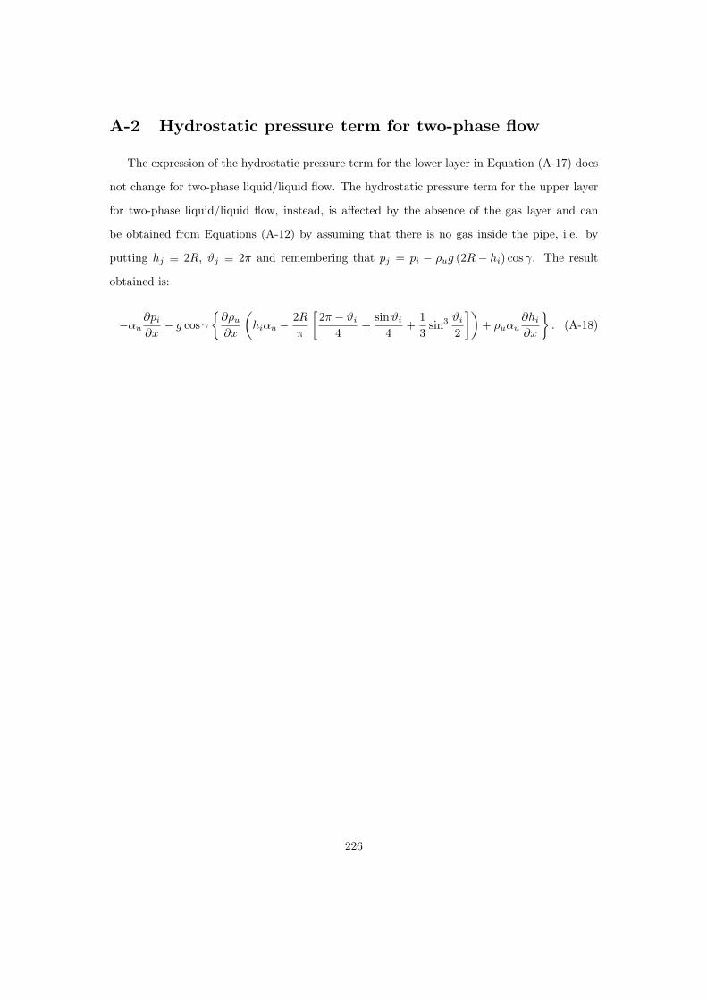
A-2 Hydrostatic pressure term for two-phase flow
The expression of the hydrostatic pressure term for the lower layer in Equation (A-17) does
not change for two-phase liquid/liquid flow. The hydrostatic pressure term for the upper layer
for two-phase liquid/liquid flow, instead, is affected by the absence of the gas layer and can
be obtained from Equations (A-12) by assuming that there is no gas inside the pipe, i.e. by
putting hj ≡ 2R, ϑj ≡ 2π and remembering that pj = pi − ρug (2R− hi) cos γ. The result
obtained is:
−αu∂pi
∂x− g cos γ
∂ρu
∂x
(hiαu − 2R
π
[2π − ϑi
4+
sinϑi
4+
13
sin3 ϑi
2
])+ ρuαu
∂hi
∂x
. (A-18)
226

Appendix B. Drift flux equations for liquid mixture
The continuity equation for the liquid mixture can be obtained from the summation of the
continuity equations of the two layers (Equations (5.3) and (5.4)):
∂ (ρuαu + ρlαl)∂t
+∂ (ρuuuαu + ρlulαl)
∂x= 0. (B-1)
It is assumed in Equation (B-1) that the gas phase does not entrain liquid drops. Keeping in
mind that:
ρMαM = ρuαu + ρlαl (B-2)
uu = uM + clus (B-3)
ul = uM − (1− cl) us (B-4)
cl =αwρw + βoρo
αMρM=
αlρl
αMρM, (B-5)
and substituting into Equation (B-1) one obtains:
∂ (ρMαM )∂t
+∂ (ρMuMαM )
∂x= 0. (B-6)
The momentum equation for the liquid mixture can be obtained by adding together the mo-
mentum equations for the layers (Equations (5.6) and (5.7)). Adding together the LHS of the
equations one obtains:
∂
∂t[ρuαuuu + ρlαlul] +
∂
∂x
[ρuαuu2
u + ρlαlu2l
], (B-7)
or, equivalently,
∂
∂t[ρuαu (uM + clus) + ρlαl (uM − (1− cl)us)] +
∂
∂x
[ρuαu (uM + clus)
2 +
+ρlαl (uM − (1− cl)us)2]. (B-8)
227

Expanding the parentheses in Equation (B-8) one finally obtains:
∂ (ρMαMuM )∂t
+∂
(ρMαMu2
M
)
∂x− Ω, (B-9)
being:
Ω = − ∂
∂x
[αlρlαuρu
αMρMu2
s
]. (B-10)
The pressure at the interface between the liquid layers is related to the pressure at the interface
between the gas and the liquid by the hydrostatic relation:
pi = pj + ρug (hj − hi) cos γ. (B-11)
Differentiating Equation (B-11) one obtains:
∂pi
∂x=
∂pj
∂x+ g cos γ
[∂ρu
∂x(hj − hi) + ρu
(∂hj
∂x− ∂hi
∂x
)]. (B-12)
Inserting Equation (B-12) into Equation (5.7) and adding together the RHSs of Equations (5.6)
and (5.7) one obtains the RHS of the momentum equation for the total liquid mass in the form:
−αM∂pj
∂x− αMρMg cos γ
∂hj
∂x− αMρMg sin γ − τWuSu
A− τWlSl
A+
τjSj
A+ Ψ, (B-13)
where
Ψ = αM (ρM − ρu) g cos γ∂hj
∂x− αl (ρl − ρu) g cos γ
∂hi
∂x− αlg cos γ (hj − hi)
∂ρu
∂x+
− g cos γ∂ρu
∂x
(hjαu − 2R
π
[ϑ
4− sin ϑ
4− 1
3sin3 ϑ
2
]ϑj
ϑi
)+
− g cos γ∂ρl
∂x
(hiαl − 2R
π
[ϑ
4− sin ϑ
4− 1
3sin3 ϑ
2
]ϑi
0
).
(B-14)
228

Appendix C. Results of the de Bertodano et al. [1998] cor-
relation for entrainment rate
0 0.2 0.4 0.6 0.8 1 1.2Water superficial velocity [m/s]
0
5
10
15
20
25
30
35
40
45
50
Eow
%
Uso = 1.1 m/s experimentalUso = 1.4 m/s experimentalUso = 1.1 m/s predictionUso = 1.4 m/s prediction
Figure C-1: Oil fraction dispersed in water for oil superficial velocities Uso = 1.1 m/s andUso = 1.4 m/s (Al-Wahaibi [2006])
229

0 0.2 0.4 0.6 0.8 1 1.2Water superficial velocity [m/s]
0
5
10
15
20
25
30
35
40
45
50
Ew
o %
Uso = 1.1 m/s experimentalUso = 1.4 m/s experimentalUso = 1.1 m/s predictionUso = 1.4 m/s prediction
Figure C-2: Water fraction dispersed in oil for oil superficial velocities Uso = 1.1 m/s andUso = 1.4 m/s (Al-Wahaibi [2006])
0 10 20 30 40 50 60 70 80 90 100input water fraction %
0
10
20
30
40
50
60
Eow
%
exp - umix = 1.34 m/scalc - umix = 1.34 m/s
0 10 20 30 40 50 60 70 80 90 100input water fraction %
0
10
20
30
40
50
60
Eow
%
exp - umix = 1.5 m/scalc - umix = 1.5 m/s
Figure C-3: Oil fraction dispersed in water for UM = 1.34 m/s and UM = 1.5 m/s (Elseth[2001])
230

0 10 20 30 40 50 60 70 80 90 100input water fraction %
0
10
20
30
40
50
60
Eow
%exp - umix = 1.67 m/scalc - umix = 1.67 m/s
0 10 20 30 40 50 60 70 80 90 100input water fraction %
0102030405060
7080
Eow
%
exp - umix = 2.0 m/scalc - umix = 2.0 m/s
Figure C-4: Oil fraction dispersed in water for UM = 1.67 m/s and UM = 2.0 m/s (Elseth[2001])
0 10 20 30 40 50 60 70 80 90 100input water fraction %
0
10
20
30
40
50
60
Eow
%
exp - umix = 2.5 m/scalc - umix = 2.5 m/s
0 10 20 30 40 50 60 70 80 90 100input water fraction %
0
10
20
30
40
50
60
Eow
%
exp - umix = 3.0 m/scalc - umix = 3.0 m/s
Figure C-5: Oil fraction dispersed in water for UM = 2.5 m/s and UM = 3.0 m/s (Elseth [2001])
231
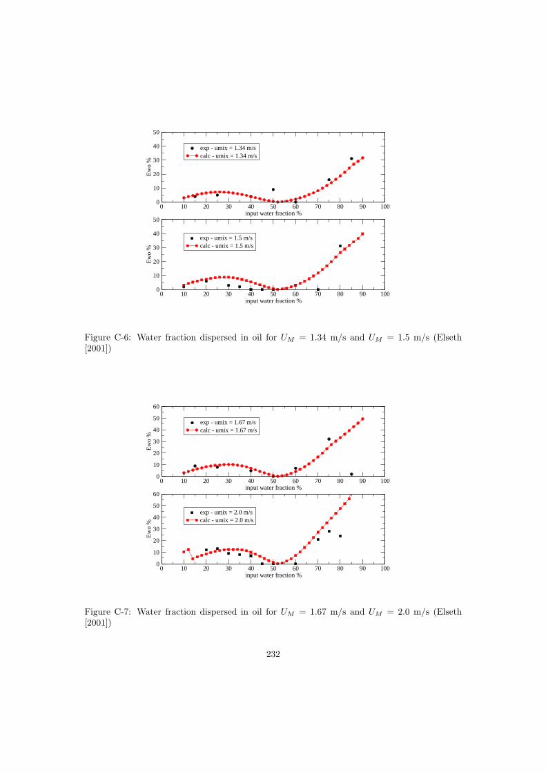
0 10 20 30 40 50 60 70 80 90 100input water fraction %
0
10
20
30
40
50
Ew
o %
exp - umix = 1.34 m/scalc - umix = 1.34 m/s
0 10 20 30 40 50 60 70 80 90 100input water fraction %
0
10
20
30
40
50
Ew
o %
exp - umix = 1.5 m/scalc - umix = 1.5 m/s
Figure C-6: Water fraction dispersed in oil for UM = 1.34 m/s and UM = 1.5 m/s (Elseth[2001])
0 10 20 30 40 50 60 70 80 90 100input water fraction %
0
10
20
30
40
50
60
Ew
o %
exp - umix = 1.67 m/scalc - umix = 1.67 m/s
0 10 20 30 40 50 60 70 80 90 100input water fraction %
0
10
20
30
40
50
60
Ew
o %
exp - umix = 2.0 m/scalc - umix = 2.0 m/s
Figure C-7: Water fraction dispersed in oil for UM = 1.67 m/s and UM = 2.0 m/s (Elseth[2001])
232
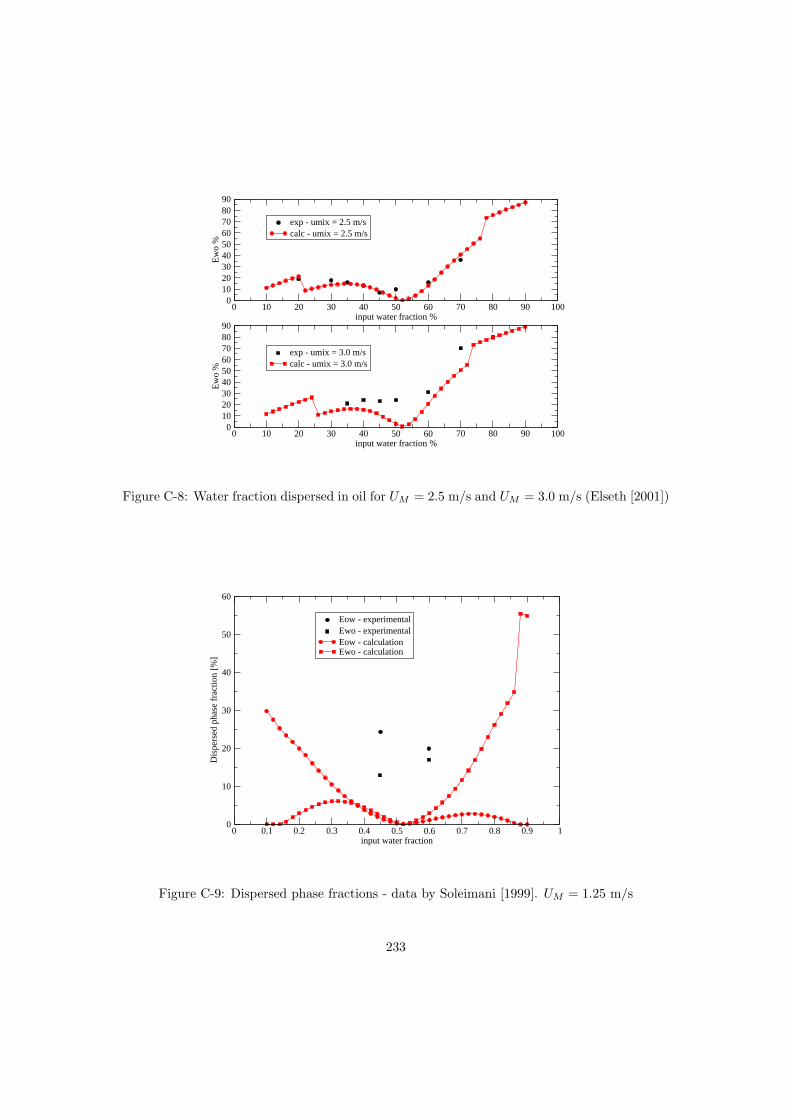
0 10 20 30 40 50 60 70 80 90 100input water fraction %
0102030405060708090
Ew
o %
exp - umix = 2.5 m/scalc - umix = 2.5 m/s
0 10 20 30 40 50 60 70 80 90 100input water fraction %
0102030405060708090
Ew
o %
exp - umix = 3.0 m/scalc - umix = 3.0 m/s
Figure C-8: Water fraction dispersed in oil for UM = 2.5 m/s and UM = 3.0 m/s (Elseth [2001])
0 0.1 0.2 0.3 0.4 0.5 0.6 0.7 0.8 0.9 1input water fraction
0
10
20
30
40
50
60
Dis
pers
ed p
hase
fra
ctio
n [%
]
Eow - experimentalEwo - experimentalEow - calculationEwo - calculation
Figure C-9: Dispersed phase fractions - data by Soleimani [1999]. UM = 1.25 m/s
233

0 0.1 0.2 0.3 0.4 0.5 0.6 0.7 0.8 0.9 1input water fraction
0
10
20
30
40
50
Eow
[%
]expcalc
0 0.1 0.2 0.3 0.4 0.5 0.6 0.7 0.8 0.9 1input water fraction
0
10
20
30
40
50
Ew
o [%
]
expcalc
Figure C-10: Dispersed phase fractions UM = 1.0 m/s - data by Lovick [2004]
0 0.1 0.2 0.3 0.4 0.5 0.6 0.7 0.8 0.9 1input water fraction
0
10
20
30
40
50
Eow
[%
]
expcalc
0 0.1 0.2 0.3 0.4 0.5 0.6 0.7 0.8 0.9 1input water fraction
0
10
20
30
40
50
60
Ew
o [%
]
expcalc
Figure C-11: Dispersed phase fractions UM = 1.5 m/s - data by Lovick [2004]
234

0 10 20 30 40 50 60 70 80 90 100input water fraction %
0
500
1000
1500
2000
2500
3000
3500
4000
4500
5000Pr
essu
re g
radi
ent [
Pa/m
]
calc - 1.8 m/scalc - 2.17 m/scalc - 2.5 m/scalc - 2.76 m/sexp - 1.8 m/sexp - 2.17 m/sexp - 2.5 m/sexp - 2.76 m/s
Figure C-12: Pressure losses by Hussain [2004] - Hand correlation
0 10 20 30 40 50 60 70 80 90 100input water fraction %
0
500
1000
1500
2000
2500
3000
3500
4000
4500
5000
Pres
sure
gra
dien
t [Pa
/m]
calc - 1.8 m/scalc - 2.17 m/scalc - 2.5 m/scalc - 2.76 m/sexp - 1.8 m/sexp - 2.17 m/sexp - 2.5 m/sexp - 2.76 m/s
Figure C-13: Pressure losses by Hussain [2004] - Blasius correlation
235

0 10 20 30 40 50 60 70 80 90 100input water fraction %
0
500
1000
1500
2000
2500
3000
3500
4000
4500
5000Pr
essu
re g
radi
ent [
Pa/m
]
calc - 1.8 m/scalc - 2.17 m/scalc - 2.5 m/scalc - 2.76 m/sexp - 1.8 m/sexp - 2.17 m/sexp - 2.5 m/sexp - 2.76 m/s
Figure C-14: Pressure losses by Hussain [2004] - Zigrang & Sylvester correlation
0 10 20 30 40 50 60 70 80 90 100input water cut %
0
500
1000
1500
2000
2500
3000
3500
4000
4500
5000
5500
6000
Pres
sure
gra
dien
t [Pa
/m]
calc - 3.0 m/scalc - 2.5 m/scalc - 2.1 m/scalc - 1.75 m/scalc - 1.5 m/scalc - 1.25 m/scalc - 1.0 m/sexp - 3.0 m/sexp - 2.5 m/sexp 2.1 m/sexp 1.75 m/sexp 1.5 m/sexp 1.25 m/sexp 1.0 m/s
Figure C-15: Pressure losses by Soleimani [1999] - Hand correlation
236
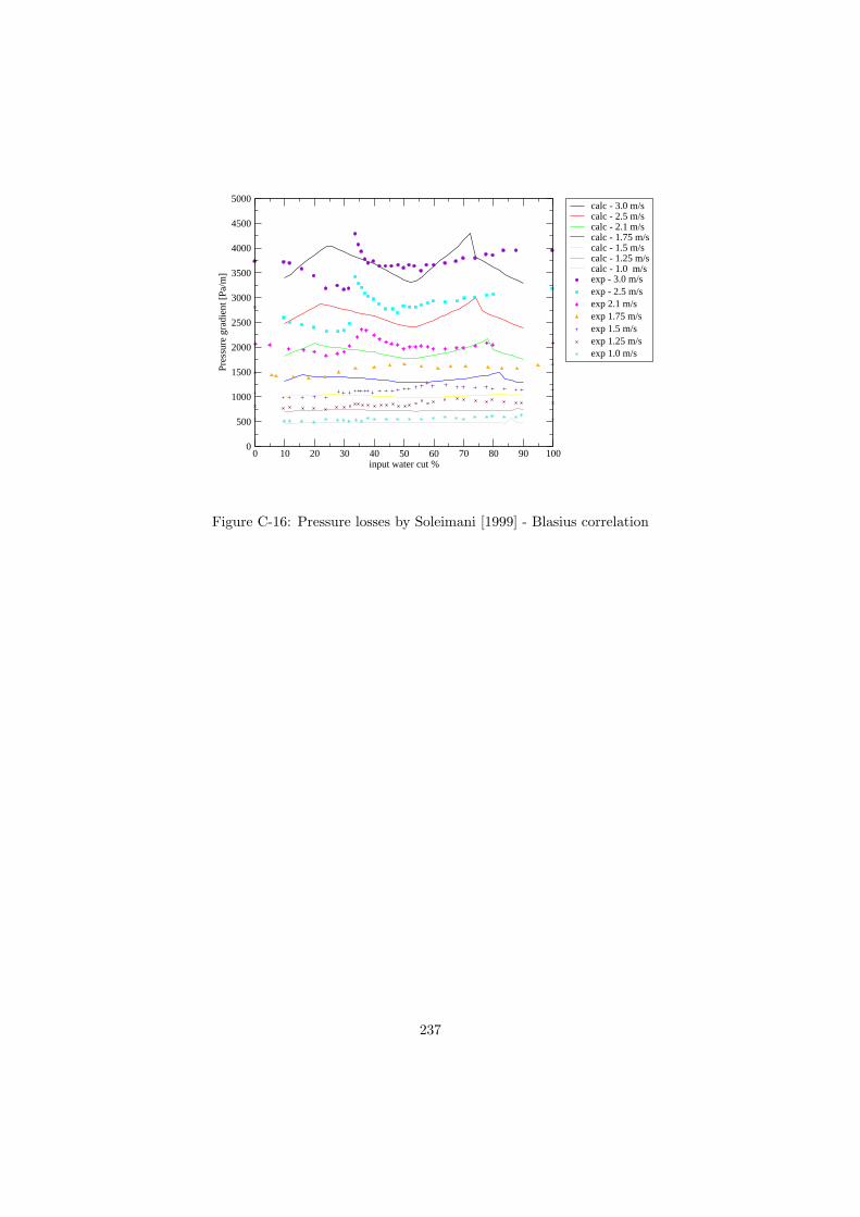
0 10 20 30 40 50 60 70 80 90 100input water cut %
0
500
1000
1500
2000
2500
3000
3500
4000
4500
5000
Pres
sure
gra
dien
t [Pa
/m]
calc - 3.0 m/scalc - 2.5 m/scalc - 2.1 m/scalc - 1.75 m/scalc - 1.5 m/scalc - 1.25 m/scalc - 1.0 m/sexp - 3.0 m/sexp - 2.5 m/sexp 2.1 m/sexp 1.75 m/sexp 1.5 m/sexp 1.25 m/sexp 1.0 m/s
Figure C-16: Pressure losses by Soleimani [1999] - Blasius correlation
237

0 10 20 30 40 50 60 70 80 90 100input water cut %
0
500
1000
1500
2000
2500
3000
3500
4000
4500
5000
Pres
sure
gra
dien
t [Pa
/m]
calc - 3.0 m/scalc - 2.5 m/scalc - 2.1 m/scalc - 1.75 m/scalc - 1.5 m/scalc - 1.25 m/scalc - 1.0 m/sexp - 3.0 m/sexp - 2.5 m/sexp 2.1 m/sexp 1.75 m/sexp 1.5 m/sexp 1.25 m/sexp 1.0 m/s
Figure C-17: Pressure losses by Soleimani [1999] - Zigrang & Sylvester correlation
238

0 10 20 30 40 50 60 70 80 90 100input water cut %
0
400
800
1200
1600
2000
2400
2800
Pres
sure
gra
dien
t [Pa
/m]
calc - 1.34 m/scalc - 1.5 m/scalc - 1.67 m/scalc - 2.0 m/scalc - 2.5 m/scalc - 3.0 m/sexp - 1.34 m/sexp - 1.5 m/sexp - 1.67 m/sexp - 2.0 m/sexp - 2.5 m/sexp - 3.0 m/s
Figure C-18: Pressure losses by Elseth [2001] - Hand correlation
239
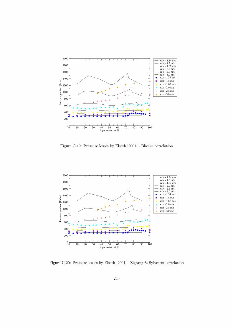
0 10 20 30 40 50 60 70 80 90 100input water cut %
0
200
400
600
800
1000
1200
1400
1600
1800
2000Pr
essu
re g
radi
ent [
Pa/m
]calc - 1.34 m/scalc - 1.5 m/scalc - 1.67 m/scalc - 2.0 m/scalc - 2.5 m/scalc - 3.0 m/sexp - 1.34 m/sexp - 1.5 m/sexp - 1.67 m/sexp - 2.0 m/sexp - 2.5 m/sexp - 3.0 m/s
Figure C-19: Pressure losses by Elseth [2001] - Blasius correlation
0 10 20 30 40 50 60 70 80 90 100input water cut %
0
200
400
600
800
1000
1200
1400
1600
1800
2000
Pres
sure
gra
dien
t [Pa
/m]
calc - 1.34 m/scalc - 1.5 m/scalc - 1.67 m/scalc - 2.0 m/scalc - 2.5 m/scalc - 3.0 m/sexp - 1.34 m/sexp - 1.5 m/sexp - 1.67 m/sexp - 2.0 m/sexp - 2.5 m/sexp - 3.0 m/s
Figure C-20: Pressure losses by Elseth [2001] - Zigrang & Sylvester correlation
240

Appendix D. Model equations - Flowcharts of the solution
procedure
Figure D-1: Model for dispersion and segregation of the phases: explicit solution scheme withlayer velocities calculated from the mixture velocity uM and the slip velocity us
241

Figure D-2: Model for dispersion and segregation of the phases: implicit solution scheme withsolution of the momentum equations for the layers velocities.
242