Embed Size (px)
Citation preview
INVESTIGATION OF ROUGH SURFACE SCATTERING OF
ELECTROMAGNETIC WAVES USING FINITE ELEMENT METHOD
A THESIS SUBMITTED TO
THE GRADUATE SCHOOL OF NATURAL AND APPLIED SCIENCES
OF
MIDDLE EAST TECHNICAL UNIVERSITY
BY
ÖZÜM EMRE AŞIRIM
IN PARTIAL FULFILLMENT OF THE REQUIREMENTS
FOR
THE DEGREE OF MASTER OF SCIENCE
IN
ELECTRICAL AND ELECTRONICS ENGINEERING
JULY 2013

Approval of the thesis:
INVESTIGATION OF ROUGH SURFACE SCATTERING OF
ELECTROMAGNETIC WAVES USING FINITE ELEMENT METHOD
submitted by Özüm Emre Aşırım in partial fulfillment of the requirements for the degree of
Master of Science in Electrical and Electronics Engineering Department, Middle East
Technical University by,
Prof. Dr. Canan Özgen
Dean, Graduate School of Natural and Applied Sciences ________________
Prof. Dr. Gönül Turhan Sayan
Head of Department, Electrical and Electronics Engineering ________________
Prof. Dr. Mustafa Kuzuoğlu
Supervisor, Electrical and Electronics Engineering Dept., METU ________________
Assoc. Prof. Dr. Özlem Özgün
Co-supervisor, Electrical and Electronics Engineering Dept., TEDU ________________
Examining Committee Members
Prof. Dr. Gönül Turhan Sayan
Electrical and Electronics Engineering Dept., METU ________________
Prof. Dr. Mustafa Kuzuoğlu
Electrical and Electronics Engineering Dept., METU ________________
Prof. Dr. Gülbin Dural
Electrical and Electronics Engineering Dept., METU ________________
Assoc. Prof. Dr. Lale Alatan
Electrical and Electronics Engineering Dept., METU ________________
Assoc. Prof. Dr. Özlem Özgün
Electrical and Electronics Engineering Dept., TEDU ________________
Date: 23.07.2013

I hereby declare that all information in this document has been obtained and
presented in accordance with academic rules and ethical conduct. I also
declare that, as required by these rules and conduct, I have fully cited and
referenced all material and results that are not original to this work.
Name, Last name :
Signature :
III
ABSTRACT
INVESTIGATION OF ROUGH SURFACE SCATTERING OF
ELECTROMAGNETIC WAVES USING FINITE ELEMENT METHOD
Aşırım, Özüm Emre
M.S. Department of Electrical and Electronics Engineering
Supervisor : Prof. Dr. Mustafa Kuzuoğlu
Co-Supervisor : Assoc. Prof. Dr. Özlem Özgün
July 2013, 152 pages
This thesis analyzes the problem of electromagnetic wave scattering from rough
surfaces using finite element method. Concepts like mesh generation and random
rough surface generation will be discussed firstly. Then the fundamental concepts
of the finite element method which are the functional form of a given partial
differential equation, implementation of the element coefficient matrices, and the
assemblage of elements will be discussed in detail. The rough surface and the
overall mesh geometry will be implemented with the functional form of the wave
equation, in the form of a global coefficient matrix using finite element method.
Along with an incident wave, boundary conditions on the rough surface will be
imposed and the scattering from different rough surfaces will be analyzed by
solving the resulting linear system of equations that is yielded by the finite element
method. The issues of wave resolution, required mesh size, and the required
computation time will also be discussed as part of the analysis.
Keywords: Rough Surface, Finite Element Method, Scattering
IV
ÖZ
BOZUK YÜZEYLERDEN ELEKTROMANYETİK DALGA SAÇILIMININ
SONLU ELEMANLAR YÖNTEMİ KULLANILARAK İNCELENMESİ
Aşırım, Özüm Emre
Yüksek Lisans, Elektrik Elektronik Mühendisliği Bölümü
Tez Yöneticisi: Prof. Dr. Mustafa Kuzuoğlu
Ortak Tez Yöneticisi: Doç. Dr. Özlem Özgün
Temmuz 2013, 152 sayfa
Bu tezde bozuk yüzeylerden saçılım problemi sonlu elemanlar yöntemi kullanılarak
incelenmektedir. Anlatımda öncelikle bozuk yüzey modellenmesi ve örgü
modellenmesi incelenecektir. Daha sonra, sonlu elemanlar yönteminin temel
içerikleri olan eleman katsayı matrisleri ve eleman birleştirilmesi gibi konular
detaylıca anlatılacaktır. Dalga denkleminin fonksiyonel formu bozuk yüzeyi içeren
örgü geometrisi ile birlikte sonlu elemanlar yöntemi kullanılarak katsayı matrisine
çevrilecektir. Bunu takiben, bozuk yüzeye gelen dalga ile birlikte bozuk yüzey
üzerindeki sınır değer problemi tanımlanacak ve bozuk yüzeyden saçılım problemi
sonlu elemanlar tekniği ile elde edilen lineer denklem sisteminin çözümü ile analiz
edilecektir. Dalga çözünürlüğü, analiz için gereken örgü boyutu, ve analiz için
gereken işlem zamanı gibi problemlerde analizde yer alacaktır.
Anahtar Kelimeler: Bozuk Yüzeyler, Sonlu Elemanlar Yöntemi, Saçılım
V

To My Parents
VI

ACKNOWLEDGMENTS
I would like to express my deepest gratitude to my supervisor Prof. Dr. Mustafa
Kuzuoğlu and co-supervisor Assoc. Prof. Dr. Özlem Özgün for their guidance,
advice, criticism, encouragements and tolerance throughout the research. Without
their support this thesis would not have been completed.
I would also like to thank my friend Mr. Mustafa Gökhan Şanal for his suggestions
and comments.
VII

TABLE OF CONTENTS
ABSTRACT………………………………………………………………………...IV
ÖZ……………………………………………………………………………………V
CHAPTER
1. INTRODUCTION……………………………………………………………………1
2. MAXWELL’S EQUATIONS AND SURFACE BOUNDARY CONDITIONS……3
2.1 Boundary conditions for a media with finite conductivity…………………. 4
2.2 Boundary conditions for a media with infinite conductivity………………...6
2.3 Boundary conditions when there is a source along the interface……………7
2.4 Summary of the boundary conditions……………………………………….7
2.5 Maxwell’s equations in anisotropic media………………………………….8
2.6 Impedance boundary conditions……………………………………………10
3. WAVE EQUATION……………………………………………………………….14
3.1 Wave equation for isotropic media………………………………………...14
3.2 Wave equation in PML (Perfectly Matched Layer) media………………..16
4. MESH GENERATION……………………………………………………………21
4.1 Mesh generation for rectangular domains………………………………...22
4.2 Mesh generation for regions with nonrectangular boundaries…………....26
4.3 Mesh refinement…………………………………………………………...30
4.4 Mesh generation for analyzing rough surface scattering…………………..33
4.5 Generating gaussian rough surfaces………………………………………39
VIII

5. BASICS OF THE TWO DIMENSIONAL
FINITE ELEMENT METHOD……………………………………………44
5.1 Converting PDEs into their functional forms……………………………45
5.2 Solution of the Laplace equation using finite element method…………..49
5.3 Solution of the wave equation using finite element method……………...59
5.4 Prescribed and free nodes of a solution region………………………….....67
5.5 Examples of 2D FEM solutions of the Helmholtz equation ……………...70
6. APPLICATION OF FEM ON ROUGH SURFACE
SCATTERING PROBLEMS……………………………………………………...73
6.1 Locally-conformal perfectly matched layer……………………………...75
6.2 Imposing boundary conditions on the rough surface……………………...79
6.3 Examples of rough surface scattering using FEM…………………………86
6.4 Comparison of FEM solutions with analytical solutions…………………107
7. FAR FIELD ANALYSIS OF THE ROUGH SURFACE
SCATTERING PROBLEM………………………………………………………122
7.1 Relation of the peak power with surface roughness………………………137
8. CONCLUSION…………………………………………………………………..150
REFERENCES……………………………………………………………………...152
IX

This page is intentionally left blank.
X
1
CHAPTER 1
INTRODUCTION
Electromagnetic waves propagate in space as stated by Maxwell’s equations. Based on the
characteristics of the medium of propagation, we may simplify the formulation of Maxwell’s
equations. The propagation of electromagnetic waves can be described in a much simpler
form when the medium of propagation is an unbounded medium that has no scatterers in it.
However this is usually not the case and we may have many scatterers in a given medium.
Therefore the propagation of electromagnetic waves in a medium that contains scattering
objects requires more detailed analysis and discussion.
The analysis and discussion of electromagnetic wave propagation in a bounded media that
contains scattering objects involves the determination of the scattered wave given an incident
wave. To determine the scattered wave from an incident wave, we focus our interest on the
shape and the structure of the scatterer. Using Maxwell’s equations based on the shape and
the constitutive parameters of the scatterer, we can determine the scattered wave.
In this thesis, we are interested in the determination of the scattered field in a media that is
bounded by another media which has a rough boundary. Therefore we are interested in a
rough surface scattering problem. In other words, our aim is to determine the scattered field
from the rough surface boundary by applying Maxwell’s equations given an incident field.
The determination of the scattered field allows us to examine its far field pattern and to
discuss the effects of surface roughness on the scattering of a given incident wave.
The effect of surface roughness on the scattered field pattern has been studied by many
scientists. It is found that as the roughness of the scattering surface increases, the far field
peak amplitude of the scattered field decreases. However there are no exact analytical
formulations that give the relation between surface roughness and the far field peak scattered
field amplitude. Furthermore, the critical roughness levels of a surface that may cause
significant or complete distortion in the far field scattered field pattern for a given incidence
angle are not very well known and there is still considerable ambiguity about “ How rough a
given rough surface really is? ”. In this thesis, our aim is to determine the amount of
distortion of a scattered field pattern for a given surface roughness and an incidence angle.
In literature, there are two approximate formulas that are called “Ament’s formula” and
“Boithias’ formula”, both of these formulas gives an idea about the relation between surface
roughness and the far field peak scattered field amplitude. However, it is still not clear which
of these two formulas is more accurate. The amount of error yielded by these two formulas is
not negligible for all incidence angles and it changes with respect to the angle of incidence.
Especially for grazing incidence angles, the amount of error increases significantly.
2
One purpose of this thesis is to determine the amount of distortion in the scattered field
pattern for different surface roughness levels and for different angles of incidence by
measuring the correlation coefficient of the rough surface scattered field patterns with that of
a flat surface scattered field pattern.
The second and the main purpose of this thesis is to numerically determine an accurate
relation between the peak amplitude of the scattered field and surface roughness. Afterwards,
our goal is to compare the determined relation with Ament’s formula and Boithias’ formula
to decide which of the two formulas is more accurate for a given surface roughness at a
specific incidence angle. We produce a table of results that will give the reader a firm idea
about the relation between the peak scattered field amplitude decay and surface roughness.
By looking at this table, one can have a better understanding of the effect of different surface
roughness levels on the far field scattered field pattern.
All of the computations in this thesis are performed by employing Finite Element Method
(FEM), which is often used for solving partial differential equations. We will utilize
Maxwell’s equations to get a second order wave equation and we will solve for a scalar
second order wave equation for the case. The solution of a second order partial
differential equation in a domain that has an arbitrary boundary can be very accurately
obtained by using FEM. In order to solve a 2D rough surface scattering problem using FEM,
one has to deal with the problem of mesh generation. Generating meshes for regions with
arbitrary boundaries will be discussed in detail. Since the scattering problem is an open
boundary problem, the domain of interest must be limited to a manageable size. This
requires the use of an absorbing boundary condition. As an absorbing boundary condition,
we will use a Perfectly Matched Layer (PML) for absorbing the outgoing waves without
reflection.
Our rough surface boundary will be lossy, which indicates that the scattering media is
conductive, therefore an impedance boundary condition on the rough surface will be
imposed by the FEM formulation. Since we are interested in the scattered field only, the
transmitted wave in the conductive medium will not be investigated.
The scattered field plots are given for different surface roughness levels and different
incidence angles for the purpose of illustration in chapter 6.
Along with the main purpose of this thesis, the necessary background for the application of
FEM on a rough surface scattering problem is discussed in very detail. If the reader is
already familiar with the FEM concept, chapter 6 and chapter 7 should be of more interest.
The essence of this thesis is mostly given in chapter 7, which discusses and illustrates the
effect of surface roughness on the far field scattered field pattern. Our computational results
are compared with Ament’s formula and Boithias’ formula and the accuracy of each formula
is tested for different surface roughness levels and for different angles of incidence.
In the conclusion chapter, the obtained results in chapter 7 are analyzed and discussed. Based
on these results, the potential for future investigations is established.
3
CHAPTER 2
MAXWELL’S EQUATIONS AND SURFACE BOUNDARY CONDITIONS
Maxwell’s equations simply describe field behaviour according to the properties of the
medium of interest. They are the summary of electromagnetic theory and are considered as
physical laws describing the relation between electric fields, magnetic fields, charge
densities and current densities. These equations were seperately found as the result of many
experiments and they are summarized by James Clerk Maxwell. Since the electric and
magnetic fields are vector quantities, these equations are also vector equations which can
be decoupled into their scalar forms for each dimension. Maxwell’s equations can be stated
in differential or integral form, here we are more interested in their differential form,
therefore only the differential forms are stated here.
The differential form of Maxwell’s equations are stated below
All of the quantities written in bold are vectors and and are scalar quantities. The
description of all quantities are given below
E = Electric field intensity (volts/meter)
H = Magnetic field intensity (amperes/meter)
D= Electric flux density (coulombs/square meter)
B= Magnetic flux density (webers/square meter)
= Impressed electric current density (amperes/square meter)
= Conduction electric current density (amperes/square meter)
= Displacement electric current density (amperes/square meter)
4
= Impressed magnetic current density (volts/square meter)
= Displacement magnetic current density (volts/square meter)
= Electric charge density (coulombs/cubic meter)
= Magnetic charge density (webers/cubic meter)
The equation of continuity can be derived directly from the Maxwell’s equations, as
follows:
( )
( )
The quantities E , H , D , B , are related through the constitutive parameters of the
media of interest. These constitutive parameters are different for each media, and they are
related with the physical properties of the material that forms the media of interest. The
constitutive relations are listed below for isotropic media
𝝐 : Permittivity of the medium (Farad/meter)
µ : Permeability of the medium (Henry/meter)
σ : Conductivity of the medium (Siemens/meter)
Since the curl operator is a first order vector differential operator, Maxwell’s equations are
first order, vector differential equations. In order to have a unique solution, differential
equations require boundary conditions. In electromagnetics, the field values of interest
must be specified across the boundaries of the solution region in order to determine a
unique solution for that region. Boundary conditions for finitely conductive media and
infinitely conductive media will be considered respectively and then they will be modified
when there are source currents or source charges at the boundaries.
2.1 Boundary conditions for a media with finite conductivity
The relationship between the two electric field intensities at the interface between two
different media is related with the unit normal vector of the interface as follows
( )
5
Where is the electric field intensity at media 2 and is the electric field intensity at
media 1 and if we consider the interface between the two media as a two dimensional
surface, is the unit normal vector pointing towards media 2.
The conductivities of media 1 and media 2 are and respectively, where
implies that both of the two media have finite conductivity.
An identical relationship is valid for the magnetic field intensities at the interface between
two finitely conductive media
( )
Both of the equations for electric and magnetic fields imply that the tangential components
of the electric and magnetic fields are continuous at an interface between two media with
finite conductivities. However if there are source charges or currents at the interface
between the two media or if either of the two media is a perfect conductor these two
equations do not hold and they must be modified. Boundary conditions for electric and
magnetic fields at perfectly conducting interfaces and for source containing interfaces will
be discussed here respectively.
The boundary condition for the electric flux densities at an interface between two finitely
conductive media is stated below
( )
This equation states that the normal components of the electric flux densities at an interface
between two finitely conductive media which have no source charges or source currents are
continuous. The same equation can be written in terms of the electric field intensities and
permittivities of the two media as
( )
Which states that the normal components of the electric field intensities at an interface
between two finitely conductive media which have no source charges or source currents are
discontinuous. This is expected since their tangential components are continuous.
Similarly the boundary condition for the magnetic flux densities at an interface between
two finitely conductive media is stated as
( )
This equation states that the normal components of the magnetic flux densities at an
interface between two finitely conductive media which have no source charges or source
currents are continuous. The same equation can be written in terms of the magnetic field
intensities and permeabilities of the two media as
( )
Which states that the normal components of the magnetic field intensities at an interface
between two finitely conductive media which have no source charges or source currents are
discontinuous. This is expected since their tangential components are continuous.
6
2.2 Boundary conditions for a media with infinite conductivity
The previously-stated four boundary conditions which are given for a finitely conductive
media must be modified if one of the media is of infinite conductivity or if there are source
charges or currents at the interface between the two media. Assume that media 1 has
infinite conductivity, this implies that =0, so the boundary condition for the electric
field intensities is modified as
,
Which states that the tangential component of the total electric field intensity is zero at
the interface given that media 1 is a perfect electric conductor and .
From the first equation of Maxwell, we can find that also, since
Since medium1 is a perfect electric conductor, there will be an induced electric current
density and an induced electric charge density along the interface between media 1 and
media 2, in that case the boundary condition for the magnetic field intensities must be
modified to account for the induced charges as stated below
( )
= Induced electric current density (amperes/square meter)
Which states that the tangential component of the total magnetic field intensity , is
equal to the induced electric current density along the interface given that media 1 is a
perfect electric conductor and .
The boundary condition for the electric flux densities at a perfectly conductive interface
between two media, where media 1 is a perfect electric conductor is given as
( )
= Surface electric charge density (coulombs/square meter)
These equations state that the normal components of the electric flux density and electric
field intensity are discontinuous at a perfectly conducting interface, where an induced
surface charge density exists.
7
2.3 Boundary conditions when there is a source along the interface (General case)
If none of the two media is a perfect electric conductor, and if there are electric and
magnetic sources existing at the boundary (or interface) , the four boundary conditions are
modified to include the impressed (source) current and charge densities as
( )
( )
( )
( )
(
)
(
)
(
)
(
)
2.4 Summary of the boundary conditions
Finitely conductive media
( )
( )
( )
( )
Infinitely conductive media
8
General case
( )
( )
( )
( )
2.5 Maxwell’s equations in anisotropic media
Maxwell’s equations for isotropic media are
Substituting into the first equation and into the second equation we get
Since these two equations are 3 dimensional vector differential equations, each of them can
be decoupled into 3 scalar differential equations as follows
(
) (
) (
)
(
) (
) (
)
9
Therefore, we seperate each vector to its {x,y,z} components
Where , and are scalars. However, for anisotropic media , and are not scalars
but they are expressed as direction dependent tensors, therefore the last 6 equations must be
modified since , and are not scalar quantities anymore and behave differently for
each component of and H.
For anisotropic media , and are expressed as
[
] µ [
] [
]
Therefore 𝝐 and µ in anisotropic media are related to and H by dot product operation
𝝐 µ.H
( )
( 𝝐 )
(𝝐 )
( )
Therefore the corresponding scalar equations for field components in anisotropic media are
(
)
(
)
(
)
( )
(
)
( )
10
( )
( )
( )
( )
( )
( )
Now let us consider the case of an anisotropic media where and are scalars and
conductivity is diagonally direction dependent
µ [
] 𝝐 [
] [
]
where is not a scalar but a diagonal tensor with , , in that
case, the corresponding scalar equations for field components become
The two examples of anisotropic media are the ionosphere and the artifical PML medium.
2.6 Impedance boundary conditions
There may be infinitely many solutions that satisfy a given differential equation, but we are
usually interested in the unique solution. For a differential equation to have a unique
solution over a given solution region, the boundary conditions of the differential equation
over the boundary of the solution region must be specified. An electromagnetic problem is
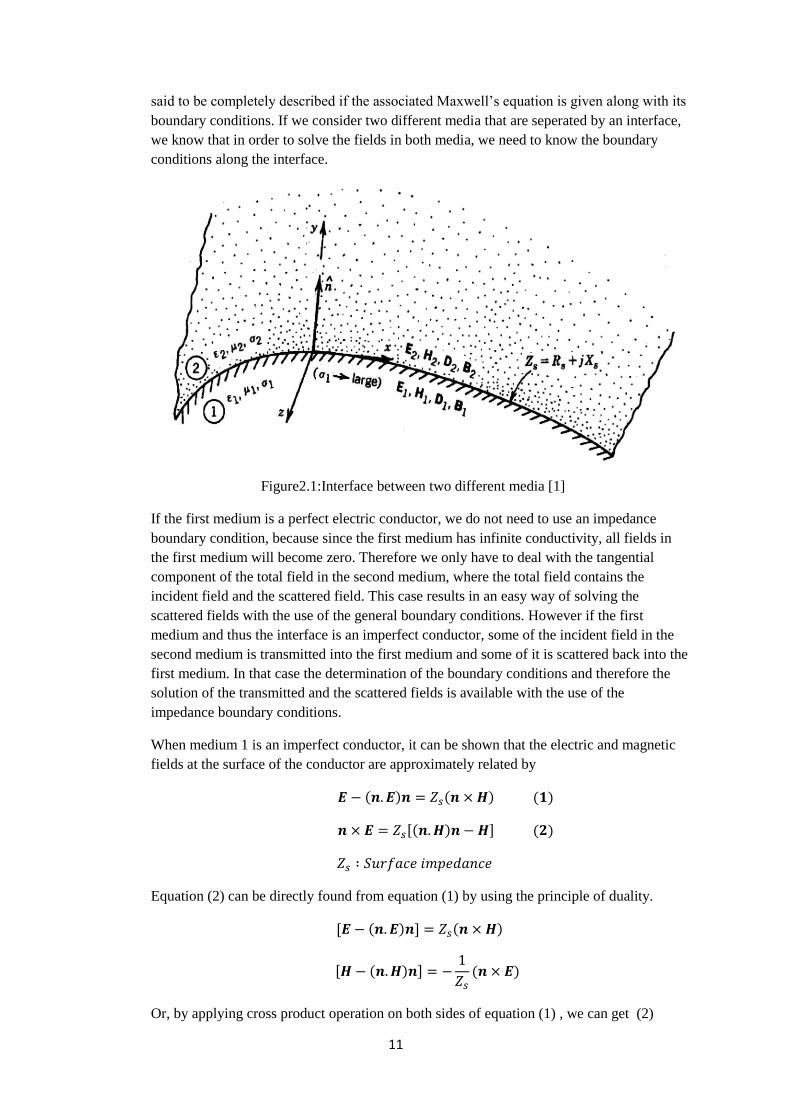
11
said to be completely described if the associated Maxwell’s equation is given along with its
boundary conditions. If we consider two different media that are seperated by an interface,
we know that in order to solve the fields in both media, we need to know the boundary
conditions along the interface.
Figure2.1:Interface between two different media [1]
If the first medium is a perfect electric conductor, we do not need to use an impedance
boundary condition, because since the first medium has infinite conductivity, all fields in
the first medium will become zero. Therefore we only have to deal with the tangential
component of the total field in the second medium, where the total field contains the
incident field and the scattered field. This case results in an easy way of solving the
scattered fields with the use of the general boundary conditions. However if the first
medium and thus the interface is an imperfect conductor, some of the incident field in the
second medium is transmitted into the first medium and some of it is scattered back into the
first medium. In that case the determination of the boundary conditions and therefore the
solution of the transmitted and the scattered fields is available with the use of the
impedance boundary conditions.
When medium 1 is an imperfect conductor, it can be shown that the electric and magnetic
fields at the surface of the conductor are approximately related by
( ) ( ) ( )
[( ) ] ( )
Equation (2) can be directly found from equation (1) by using the principle of duality.
[ ( ) ] ( )
[ ( ) ]
( )
Or, by applying cross product operation on both sides of equation (1) , we can get (2)
12
[ ( ) ] [ ]
[ ( ) ]
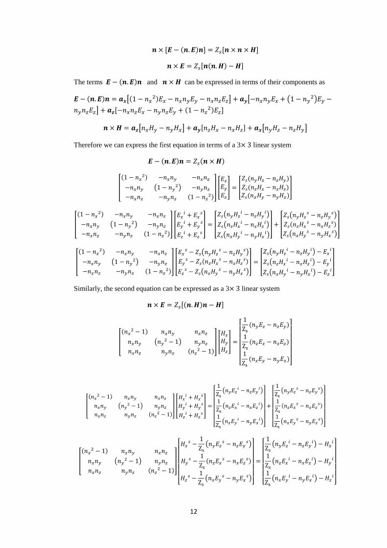
The terms ( ) and can be expressed in terms of their components as
( ) [( ) ] [ (
)
] [ ( ) ]
[ ] [ ] [ ]
Therefore we can express the first equation in terms of a 3 linear system
( ) ( )
[
( )
( )
( )
] [
] [
( )
( )
( )]
[
( )
( )
( )
] [
] [
(
)
(
)
(
)
] [
(
)
(
)
(
)
]
[
( )
( )
( )
] [
(
)
(
)
(
)
] [
(
)
(
)
(
)
]
Similarly, the second equation can be expressed as a 3 linear system
[( ) ]
[
( )
( )
( )
] [
]
[
( )
( )
( )]
[
( )
( )
( )
] [
]
[
(
)
(
)
(
)]
[
(
)
(
)
(
)
]
[
( )
( )
( )
]
[
(
)
(
)
(
)]
[
(
)
(
)
(
)
]
13
So there are 6 equations and 6 unknowns, therefore the systems can be easily solved to
yield the values of {
given the surface impedance and the
surface normal.
Note that each of the field components consists of the incident and scattered fields in
medium 2, but in medium 1, they are equal to the absorbed (transmitted) field.
The fields { in medium 2 can be expressed as
The incident field components are known, therefore we have only the scattered components
as unknowns
Since we have 6 equations at hand, all the scattered field components can be solved, we can
also solve the transmitted field components using the general boundary conditions on the
same imperfectly conducting surface
( ) ( )
( ) ( )
i) There are 3 unknown components of which are
and we have 3
equations from ( ) , therefore
can be solved.
ii) There are 3 unknown components of which are
and we have 3
equations from ( ) , therefore
can be solved.
14
CHAPTER 3
WAVE EQUATION
3.1 Wave equation for isotropic media
Although Maxwell’s four equations simply describe the field behaviour in general, the first
two equations involving E and H are coupled to each other which makes it hard to
understand the field behaviour. Instead we use some vector algebra to obtain single
variable field intensity equations for both E and H at the expense of increased order, but
the equations then become uncoupled and it becomes much easier to understand the
behaviour of the field intensities E and H. In other words we simply convert the two first-
order coupled vector differential equations into two second-order vector differential
equations each of which has a single variable and therefore not coupled to each other. To
get these single variable equations, we start with the first two of Maxwell’s equations
( )
( )
Taking the curl of both sides of these equations and assuming a homogenous medium, we
can write that
[
]
[ ] ( )
[ ] [
] [ ]
[ ] ( )
Substituting ( ) into the right side of ( ) and using the vector identity ( ) at the left side
( ) ( )
We get (6) and (7) as
( )
[
] ( )
( )
( )
Substituting Maxwell’s third equation ( ) into equation ( ) and
rearranging terms, we get
15
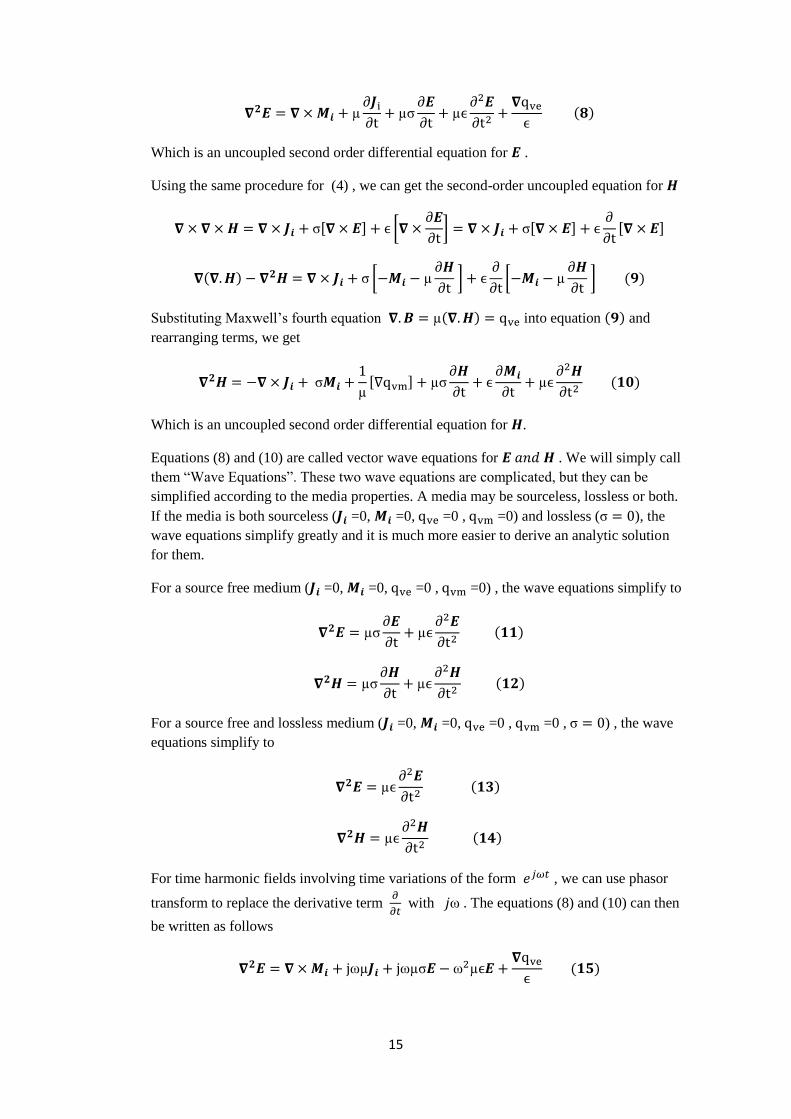
( )
Which is an uncoupled second order differential equation for .
Using the same procedure for (4) , we can get the second-order uncoupled equation for
[ ] [
] [ ]
[ ]
( ) [
]
[
] ( )
Substituting Maxwell’s fourth equation ( ) into equation ( ) and
rearranging terms, we get
[ ]
( )
Which is an uncoupled second order differential equation for .
Equations (8) and (10) are called vector wave equations for . We will simply call
them “Wave Equations”. These two wave equations are complicated, but they can be
simplified according to the media properties. A media may be sourceless, lossless or both.
If the media is both sourceless ( =0, =0, =0 , =0) and lossless ( ), the
wave equations simplify greatly and it is much more easier to derive an analytic solution
for them.
For a source free medium ( =0, =0, =0 , =0) , the wave equations simplify to
( )
( )
For a source free and lossless medium ( =0, =0, =0 , =0 , ) , the wave
equations simplify to
( )
( )
For time harmonic fields involving time variations of the form , we can use phasor
transform to replace the derivative term
with . The equations (8) and (10) can then
be written as follows
( )
16
[ ] ( )
For a source free medium ( =0, =0, =0 , =0) , ( ) and ( ) simplify to
( )
( )
[ ]
Where is called as the lossy propagation constant.
Since is complex valued, we can write it in terms of its real and imaginary parts
α : Attenuation constant (Nepers/meter)
β : Phase constant (Radians/meter)
: Lossy propagation constant
For a source free and lossless medium ( =0, =0, =0 , =0 , ) , ( ) and
( ) simplify to
( )
( )
k = √
k : Propagation constant (Radians/meter)
3.2 Wave equation in PML (Perfectly Matched Layer) media
PML is an anisotropic, lossy medium that is used to terminate the computational region for
computer memory consideration. It is commonly used in scattering and radiation problems
to limit the size of the computational medium and to simulate the computational solution as
if the computational medium size is infinity. This is achieved by adjusting the parameters
of the PML media such that the outer reflections are minimized so that the computational
solution tends to the actual analytical one.
Since PML is a lossy medium, the wave that enters the PML is completely absorbed after a
certain depth which is related with the wavelength of the incident wave. Remembering the
vector wave equations in lossy media and considering cartesian coordinates for analysis,
we can write the scalar {x,y,z} components of the vector wave equations in a lossy medium
as
( ) ( ) ( ) ( )
17
( ) ( ) ( ) ( )
( ) ( ) ( ) ( )
( ) ( ) ( ) ( )
( ) ( ) ( ) ( )
( ) ( ) ( ) ( )
Which can be coupled into their vector forms that are previously described, as follows
[ ]
( )
α : Attenuation constant (Nepers/meter)
β : Phase constant (Radians/meter)
The lossy and anisotropic nature of the PML dictates that its conductivity tensor must not
be a scalar one. The conductivity tensor of the PML is a diagonal matrix with parameters
and , but the permeability ( ) and the permittivity ( ) of the PML medium are
treated as scalars and must have appropriate values related with the electric and magnetic
conductivities of the PML to ensure reflectionless transmission of the incident wave into
the PML medium.
In a 3D PML, we have the following electric and magnetic conductivity tensors
[
] [
]
In a 2D PML, these tensors are expressed as
[
] [
]
We will deal with a 2D PML medium, therefore the conductivity tensors will be our
concern, but we must choose
such that there are no reflections from the
PML boundaries. In Berenger’s journal [2] it is suggested that we must choose the values
of the conductivities such that they satisfy the below relationships
Where and are the permittivity and permeability of free space respectively, assuming
that the computational medium which is surrounded by the PML, is simply free space.
18
Using Maxwell’s equations, we can derive the vector wave equations that are valid inside
the PML medium, since the perfectly matched layer is an artificial medium that is created
for absorbing the outgoing waves, inside the PML medium we have
=0, =0, =0 , =0
The first two equations of Maxwell can be written here as
( )
( )
Taking the curl of both sides of the equations we have
[ ] [
] [ ]
[ ] ( )
[ ] [
] [ ]
[ ] ( )
First let us deal with (3) to determine the wave equation for
( ) ( )
( ) [ ]
[ ] ( )
Taking the phasor transform of (6) we get (7) as
( ) [ ] [ ] ( )
[ ] [ ] ( )
Substituting (2) into (8) and using the vector identity [ ] [ ] , we get
[ ] [ ] ( )
(
) (
) (
) ( )
[ ] ( )
[ ] ( )
Equation 12 can be written in terms of its components as
( ) ( ) ( ) ( )
19
( ) ( ) ( ) ( )
( ) ( ) ( ) ( )
Where the coefficients
are the propagation constants along x, y and z
directions respectively.
An identical procedure is used to derive the wave equation for , therefore the wave
equation for has exactly the same form as (12). But instead of going through the same
procedure to derive the wave equation for , one can use the principle of duality. The
dual of (12) yields
[ ] ( )
Equation 13 can be written in terms of its components as
( ) ( ) ( )
( )
( ) ( ) ( )
( )
( ) ( ) ( )
( )
Where the coefficients
are the propagation constants along x,y and z
directions respectively.
The PML must have a certain depth to prevent outer reflections by attenuating the outgoing
waves. The depth of the PML is related with the wavelength of the incident wave. As the
depth of the PML increases, the accuracy of preventing outer reflections also increases,
however increasing the depth of the PML also increases the required computer memory.
Therefore appropriate lower and upper limits must be determined to effectively minimize
outer layer reflections by using minimum amount of computer memory.
20
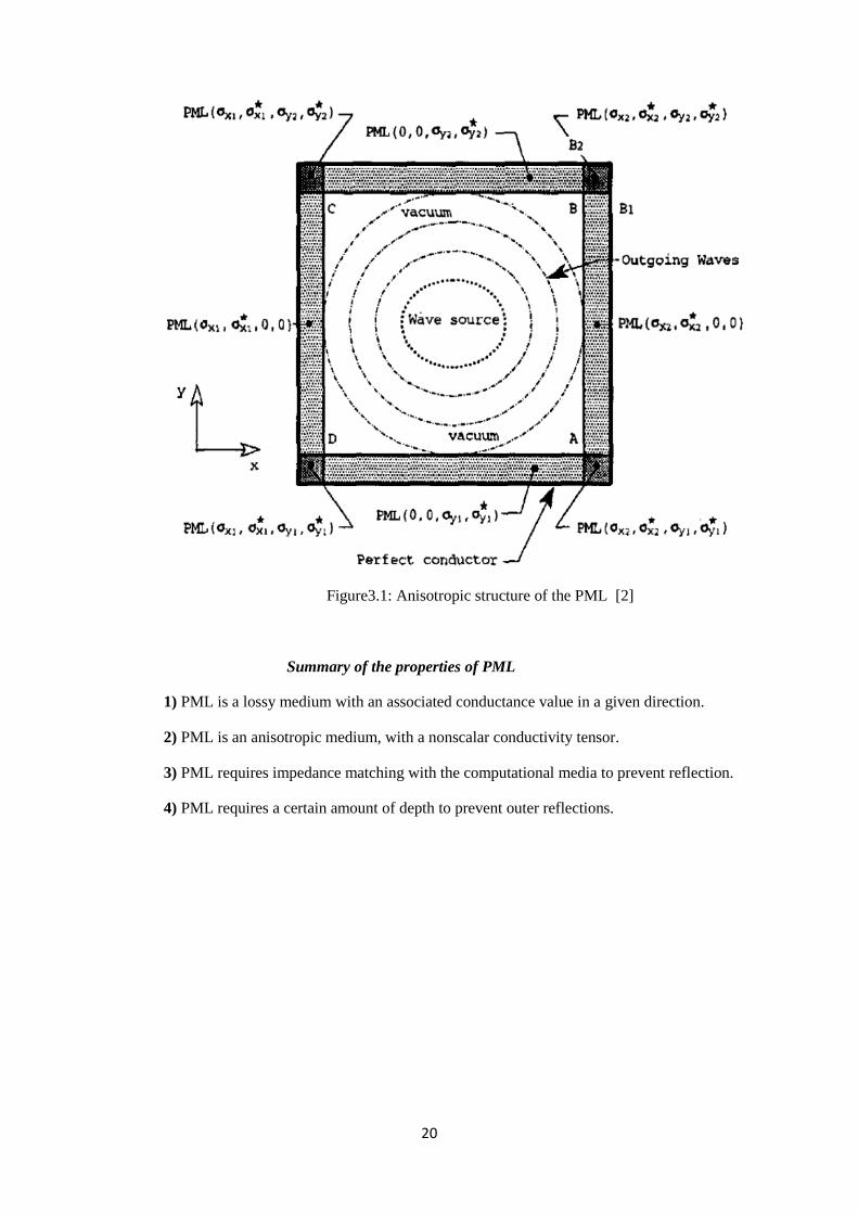
Figure3.1: Anisotropic structure of the PML [2]
Summary of the properties of PML
1) PML is a lossy medium with an associated conductance value in a given direction.
2) PML is an anisotropic medium, with a nonscalar conductivity tensor.
3) PML requires impedance matching with the computational media to prevent reflection.
4) PML requires a certain amount of depth to prevent outer reflections.
21
CHAPTER 4
MESH GENERATION
The finite element method requires the domain of interest to be discretized by a number of
elements, the accuracy of the finite element method depends strongly on how accurately
we have discretized the entire domain, i.e., the solution region. One of the biggest problems
in the finite element method is to discretize the solution region accurately. The accuracy
depends on the number of elements used and how accurately the discretized solution region
resembles the actual solution region.
Since increasing the number of elements yields more accurate solutions, we generally
require a large number of elements to discretize the region of interest. This requires a huge
data preperation step for the geometry of the problem and for the elements in the solution
region, since the coordinates of the boundary of the solution region and each of the
elements must be given as inputs to the computer program. For problems requiring very
accurate solutions we may have to use thousands of elements and for complex solution
regions we may have to use even more. Thus manual data entry for domain discretization,
which is usually called mesh generation, requires huge effort and too much time
consumption and they are very likely to yield results with serious errors. That is why we
come up with automatic mesh generation algorithms, which effectively, systematically and
quickly discretize the region of interest to a specified number of elements. Using automatic
mesh generation algorithms with different levels of automation we can greatly decrease the
amount of necessary data entry to describe the problem at hand. Another big advantage is
that since the process is now computer automized, calculation errors due to human
imperfection become eliminated. Utilizing mesh generation algorithms with the modern
tools of computer graphics, we can visualize the solutions of a given problem on a
specified domain.
There are different mesh generation algorithms in literature. These mesh generation
algorithms are created by considering the computational time efficiency and the complexity
of the solution region. A difficulty arises when the solution region is not a rectangular, but
an arbitrary solution region. Another problem in mesh generation is the computational time
required to assemble each element in the solution region due to a large number of elements.
Taking this fact into account, an optimization must be made between the number of
elements used and the time spent for computation by checking the convergence of the
computed solutions. Today’s mesh generation programs use thousands of elements to
discretize very complex domains involved in applications like structural analysis and
electromagnetics in a very time efficient manner. Most basically computational time
efficiency can be increased by efficient global node numbering and using an efficient
element assembling algorithm as will be discussed later. We will consider here three basic
mesh generation algorithms which involves
22
1) Mesh generation for rectangular regions.
2) Mesh generation for nonrectangular regions with curved boundaries.
3) Mesh refinement for computational accuracy.
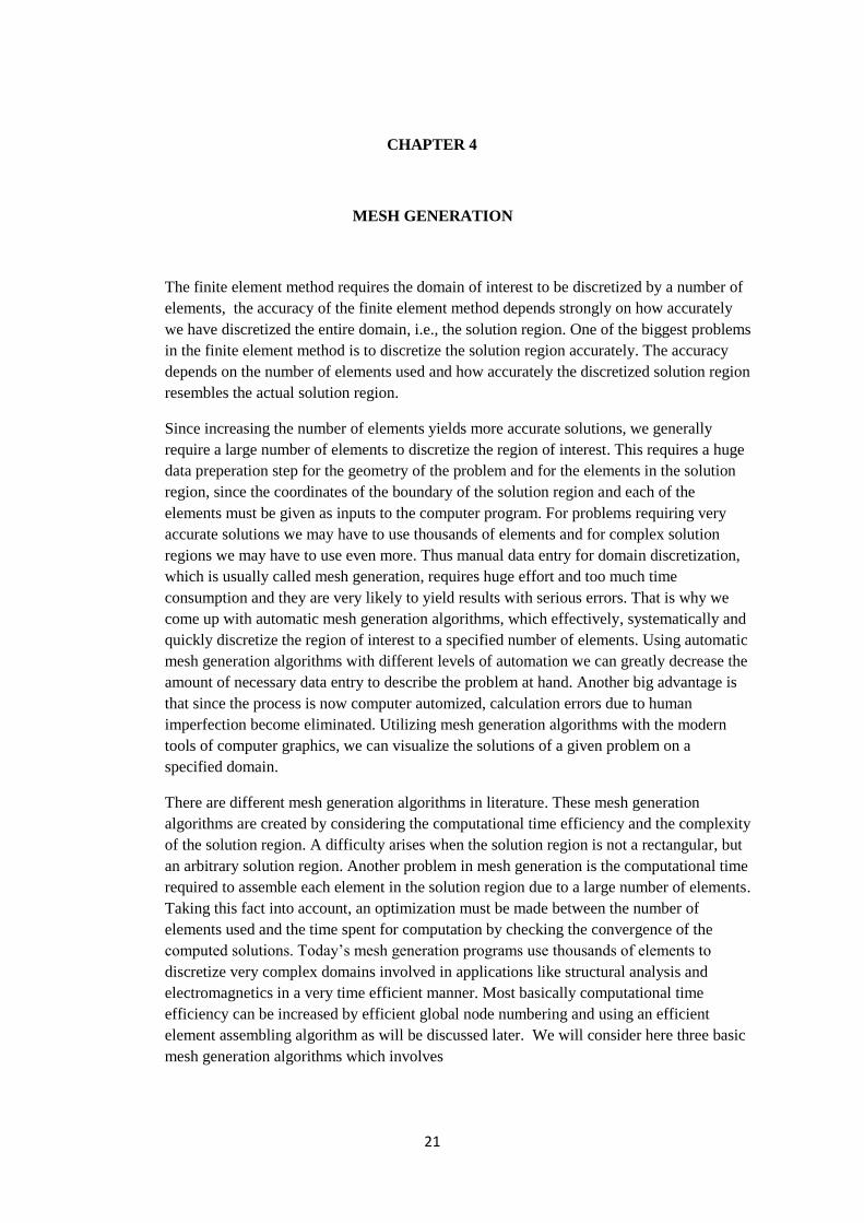
The commonly used element for discretization is a triangle, since triangles easily fit to
curved boundaries. Quadrilaterals can also be used for discretization, but since a
quadrilateral can be split into two triangles and triangles fit better to curved boundaries,
people prefer discretizing with triangles. Different types of elements (triangle,
quadrilateral) can be used at the same solution region for discretization, but this will
increase computational complexity. So, it is better to use only one type of element in a
given solution region, which are usually triangles. Discretization requires that the elements
must not overlap with each other.
Figure 4.1 : Discretization of a region enclosed by a circle [3]
4.1 Mesh generation for rectangular domains
If we are dealing with a rectangular geometry of size a x b , the first thing to do is to divide
the solution region into smaller rectangles, then these rectangles are divided into 2, each of
which are triangular elements.The number of elements used in the solution region depends
on how we divide the x and y directions. The more divisions we use in x and y directions,
the more the number of elements becomes.
-1 -0.5 0 0.5-0.8
-0.6
-0.4
-0.2
0
0.2
0.4
0.6
23
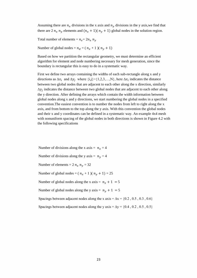
Assuming there are divisions in the x axis and divisions in the y axis,we find that
there are 2 elements and ( )( ) global nodes in the solution region.
Total number of elements = = 2
Number of global nodes = = ( + 1 )( )
Based on how we partition the rectangular geometry, we must determine an efficient
algorithm for element and node numbering necessary for mesh generation, since the
boundary is rectangular this is easy to do in a systematic way.
First we define two arrays containing the widths of each sub-rectangle along x and y
directions as ∆ and ∆ where {i,j}={1,2,3,…,N}, here ∆ indicates the distance
between two global nodes that are adjacent to each other along the x direction, similarly
∆ indicates the distance between two global nodes that are adjacent to each other along
the y direction. After defining the arrays which contain the width information between
global nodes along x and y directions, we start numbering the global nodes in a specified
convention.The easiest convention is to number the nodes from left to right along the x
axis, and from bottom to the top along the y axis. With this convention the global nodes
and their x and y coordinates can be defined in a systematic way. An example 4x4 mesh
with nonuniform spacing of the global nodes in both directions is shown in Figure 4.2 with
the following specifications
Number of divisions along the x axis = = 4
Number of divisions along the y axis = = 4
Number of elements = 2 = 32
Number of global nodes = ( + 1 )( ) = 25
Number of global nodes along the x axis = 5
Number of global nodes along the y axis = 5
Spacings between adjacent nodes along the x axis = ∆x = {0.2 , 0.5 , 0.3 , 0.6}
Spacings between adjacent nodes along the y axis = ∆y = {0.4 , 0.2 , 0.5 , 0.5}
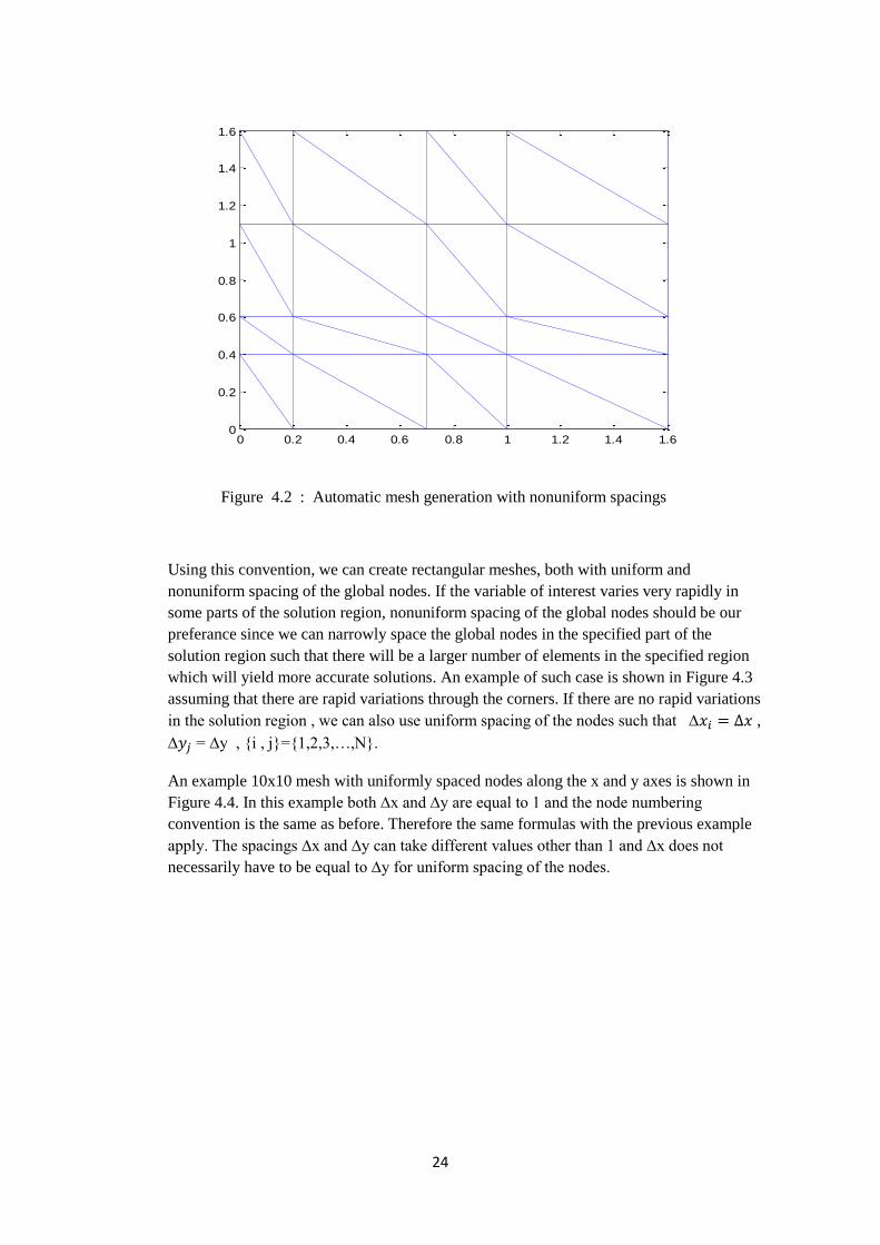
24
Figure 4.2 : Automatic mesh generation with nonuniform spacings
Using this convention, we can create rectangular meshes, both with uniform and
nonuniform spacing of the global nodes. If the variable of interest varies very rapidly in
some parts of the solution region, nonuniform spacing of the global nodes should be our
preferance since we can narrowly space the global nodes in the specified part of the
solution region such that there will be a larger number of elements in the specified region
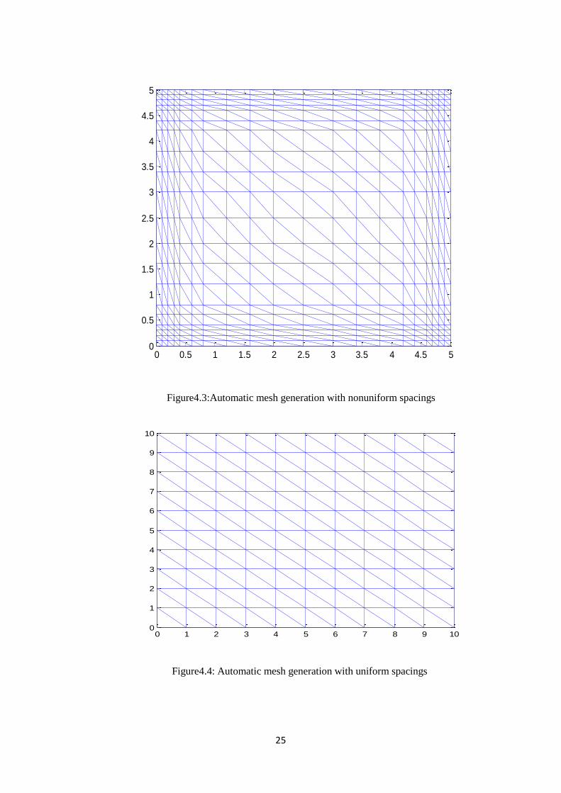
which will yield more accurate solutions. An example of such case is shown in Figure 4.3
assuming that there are rapid variations through the corners. If there are no rapid variations
in the solution region , we can also use uniform spacing of the nodes such that ∆ ,
∆ = ∆y , {i , j}={1,2,3,…,N}.
An example 10x10 mesh with uniformly spaced nodes along the x and y axes is shown in
Figure 4.4. In this example both ∆x and ∆y are equal to 1 and the node numbering
convention is the same as before. Therefore the same formulas with the previous example
apply. The spacings ∆x and ∆y can take different values other than 1 and ∆x does not
necessarily have to be equal to ∆y for uniform spacing of the nodes.
0 0.2 0.4 0.6 0.8 1 1.2 1.4 1.60
0.2
0.4
0.6
0.8
1
1.2
1.4
1.6
25
Figure4.3:Automatic mesh generation with nonuniform spacings
Figure4.4: Automatic mesh generation with uniform spacings
0 0.5 1 1.5 2 2.5 3 3.5 4 4.5 50
0.5
1
1.5
2
2.5
3
3.5
4
4.5
5
0 1 2 3 4 5 6 7 8 9 100
1
2
3
4
5
6
7
8
9
10
26
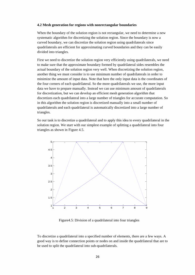
4.2 Mesh generation for regions with nonrectangular boundaries
When the boundary of the solution region is not rectangular, we need to determine a new
systematic algorithm for discretizing the solution region. Since the boundary is now a
curved boundary, we can discretize the solution region using quadrilaterals since
quadrilaterals are efficient for approximating curved boundaries and they can be easily
divided into triangles.
First we need to discretize the solution region very efficiently using quadrilaterals, we need
to make sure that the approximate boundary formed by quadrilateral sides resembles the
actual boundary of the solution region very well. When discretizing the solution region,
another thing we must consider is to use minimum number of quadrilaterals in order to
minimize the amount of input data. Note that here the only input data is the coordinates of
the four corners of each quadrilateral. So the more quadrilaterals we use, the more input
data we have to prepare manually. Instead we can use minimum amount of quadrilaterals
for discretization, but we can develop an efficient mesh generation algorithm that
discretizes each quadrilateral into a large number of triangles for accurate computation. So
in this algorithm the solution region is discretized manually into a small number of
quadrilaterals and each quadrilateral is automatically discretized into a large number of
triangles.
So our task is to discretize a quadrilateral and to apply this idea to every quadrilateral in the
solution region. We start with our simplest example of splitting a quadrilateral into four
triangles as shown in Figure 4.5.
Figure4.5: Division of a quadrilateral into four triangles
To discretize a quadrilateral into a specified number of elements, there are a few ways. A
good way is to define connection points or nodes on and inside the quadrilateral that are to
be used to split the quadrilateral into sub-quadrilaterals.
1 2 3 4 5 6 7 8 91
1.5
2
2.5
3
3.5
4
4.5
5
27
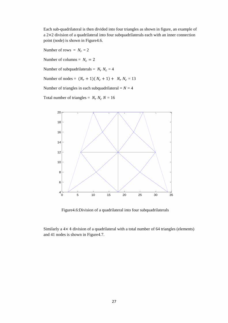
Each sub-quadrilateral is then divided into four triangles as shown in figure, an example of
a 2 2 division of a quadrilateral into four subquadrilaterals each with an inner connection
point (node) is shown in Figure4.6.
Number of rows = = 2
Number of columns =
Number of subquadrilaterals = = 4
Number of nodes = ( )( ) = 13
Number of triangles in each subquadrilateral = = 4
Total number of triangles = = 16
Figure4.6:Division of a quadrilateral into four subquadrilaterals
Similarly a 4 division of a quadrilateral with a total number of 64 triangles (elements)
and 41 nodes is shown in Figure4.7.
0 5 10 15 20 25 30 354
6
8
10
12
14
16
18
20
28
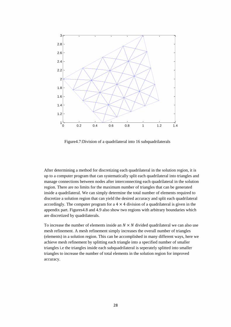
Figure4.7:Division of a quadrilateral into 16 subquadrilaterals
After determining a method for discretizing each quadrilateral in the solution region, it is
up to a computer program that can systematically split each quadrilateral into triangles and
manage connections between nodes after interconnecting each quadrilateral in the solution
region. There are no limits for the maximum number of triangles that can be generated
inside a quadrilateral. We can simply determine the total number of elements required to
discretize a solution region that can yield the desired accuracy and split each quadrilateral
accordingly. The computer program for a division of a quadrilateral is given in the
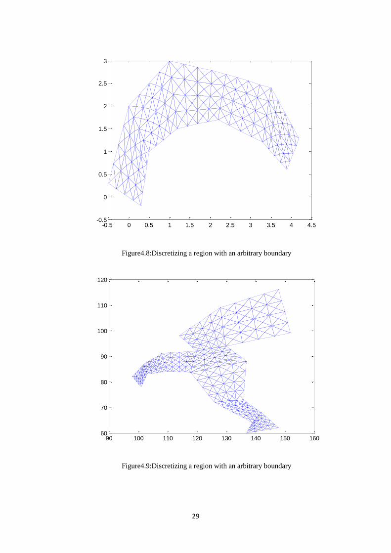
appendix part. Figures4.8 and 4.9 also show two regions with arbitrary boundaries which
are discretized by quadrilaterals.
To increase the number of elements inside an divided quadrilateral we can also use
mesh refinement. A mesh refinement simply increases the overall number of triangles
(elements) in a solution region. This can be accomplished in many different ways, here we
achieve mesh refinement by splitting each triangle into a specified number of smaller
triangles i.e the triangles inside each subquadrilateral is seperately splitted into smaller
triangles to increase the number of total elements in the solution region for improved
accuracy.
0 0.2 0.4 0.6 0.8 1 1.2 1.41
1.2
1.4
1.6
1.8
2
2.2
2.4
2.6
2.8
3
29
Figure4.8:Discretizing a region with an arbitrary boundary
Figure4.9:Discretizing a region with an arbitrary boundary
-0.5 0 0.5 1 1.5 2 2.5 3 3.5 4 4.5-0.5
0
0.5
1
1.5
2
2.5
3
90 100 110 120 130 140 150 16060
70
80
90
100
110
120
30
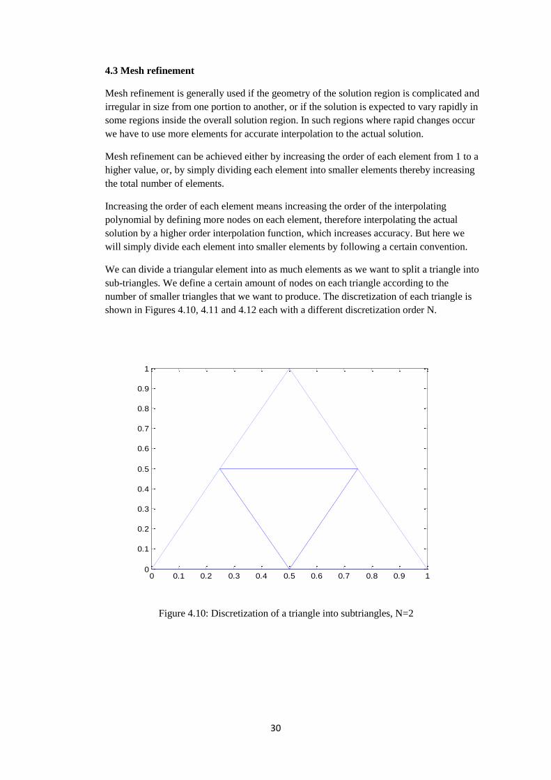
4.3 Mesh refinement
Mesh refinement is generally used if the geometry of the solution region is complicated and
irregular in size from one portion to another, or if the solution is expected to vary rapidly in
some regions inside the overall solution region. In such regions where rapid changes occur
we have to use more elements for accurate interpolation to the actual solution.
Mesh refinement can be achieved either by increasing the order of each element from 1 to a
higher value, or, by simply dividing each element into smaller elements thereby increasing
the total number of elements.
Increasing the order of each element means increasing the order of the interpolating
polynomial by defining more nodes on each element, therefore interpolating the actual
solution by a higher order interpolation function, which increases accuracy. But here we
will simply divide each element into smaller elements by following a certain convention.
We can divide a triangular element into as much elements as we want to split a triangle into
sub-triangles. We define a certain amount of nodes on each triangle according to the
number of smaller triangles that we want to produce. The discretization of each triangle is
shown in Figures 4.10, 4.11 and 4.12 each with a different discretization order N.
Figure 4.10: Discretization of a triangle into subtriangles, N=2
0 0.1 0.2 0.3 0.4 0.5 0.6 0.7 0.8 0.9 10
0.1
0.2
0.3
0.4
0.5
0.6
0.7
0.8
0.9
1
31
Figure 4.11:Discretization of a triangle into subtriangles, N=3
Figure4.12:Discretization of a triangle into subtriangles, N=4
0 0.1 0.2 0.3 0.4 0.5 0.6 0.7 0.8 0.9 10
0.1
0.2
0.3
0.4
0.5
0.6
0.7
0.8
0.9
1
0 0.1 0.2 0.3 0.4 0.5 0.6 0.7 0.8 0.9 10
0.1
0.2
0.3
0.4
0.5
0.6
0.7
0.8
0.9
1
32
Discretization Order Number Of Nodes Number Of Elements
1 3 1
2 6 4
3 10 9
4 15 16
5 21 25
6 28 36
. . .
. . .
. . .
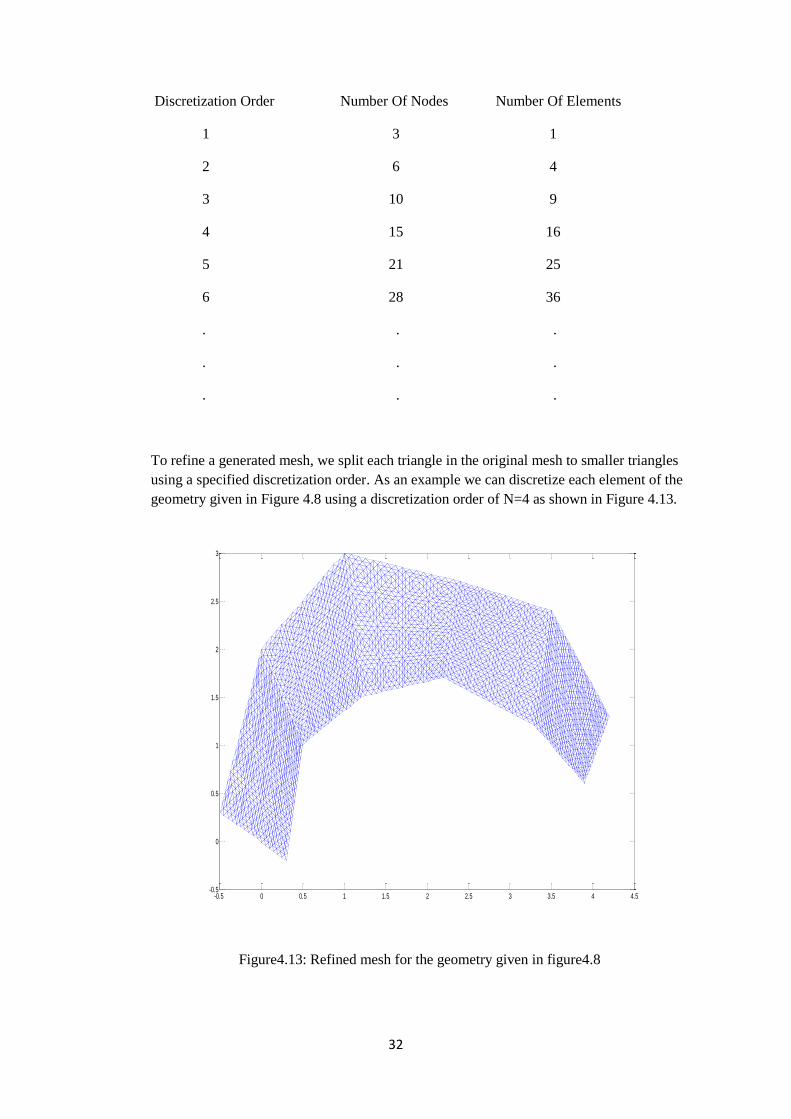
To refine a generated mesh, we split each triangle in the original mesh to smaller triangles
using a specified discretization order. As an example we can discretize each element of the
geometry given in Figure 4.8 using a discretization order of N=4 as shown in Figure 4.13.
Figure4.13: Refined mesh for the geometry given in figure4.8
-0.5 0 0.5 1 1.5 2 2.5 3 3.5 4 4.5-0.5
0
0.5
1
1.5
2
2.5
3
33
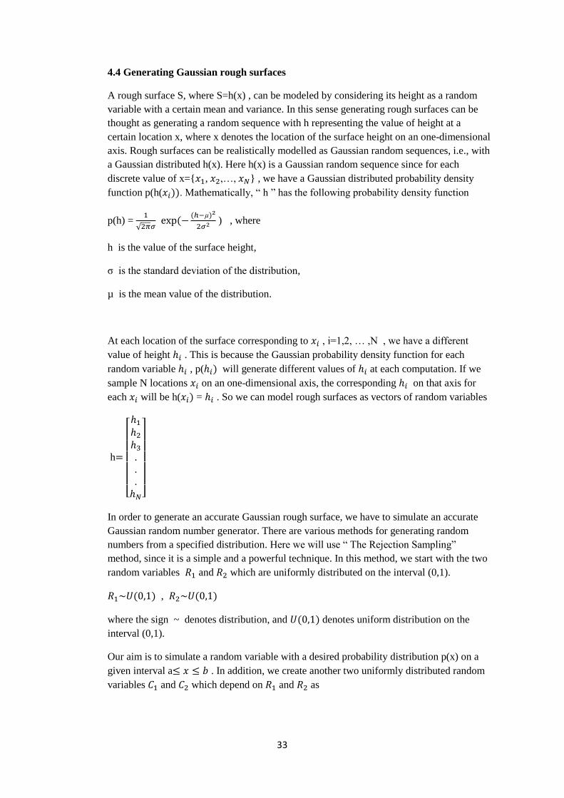
4.4 Generating Gaussian rough surfaces
A rough surface S, where S=h(x) , can be modeled by considering its height as a random
variable with a certain mean and variance. In this sense generating rough surfaces can be
thought as generating a random sequence with h representing the value of height at a
certain location x, where x denotes the location of the surface height on an one-dimensional
axis. Rough surfaces can be realistically modelled as Gaussian random sequences, i.e., with
a Gaussian distributed h(x). Here h(x) is a Gaussian random sequence since for each
discrete value of x={ , ,…, } , we have a Gaussian distributed probability density
function p(h( )). Mathematically, “ h ” has the following probability density function
p(h) =
√ (
( )
) , where
h is the value of the surface height,
is the standard deviation of the distribution,
µ is the mean value of the distribution.
At each location of the surface corresponding to , i=1,2, … ,N , we have a different
value of height . This is because the Gaussian probability density function for each
random variable , p( ) will generate different values of at each computation. If we
sample N locations on an one-dimensional axis, the corresponding on that axis for
each will be h( ) = . So we can model rough surfaces as vectors of random variables
h
[
]
In order to generate an accurate Gaussian rough surface, we have to simulate an accurate
Gaussian random number generator. There are various methods for generating random
numbers from a specified distribution. Here we will use “ The Rejection Sampling”
method, since it is a simple and a powerful technique. In this method, we start with the two
random variables and which are uniformly distributed on the interval (0,1).
( ) , ( )
where the sign ~ denotes distribution, and ( ) denotes uniform distribution on the
interval (0,1).
Our aim is to simulate a random variable with a desired probability distribution p(x) on a
given interval a . In addition, we create another two uniformly distributed random
variables and which depend on and as
34
( ) , ( )
( ) ( ( ) )
The algorithm accepts those values of as samples of the probability distribution p(x) ,
which satisfy the inequality
( )
and those do not, are rejected. Basically in the rejection sampling technique, the values of
that lie above the curve of the desired probability distribution are rejected, and the ones
that are on or below the curve of the desired distribution are accepted as samples of the
desired distribution.
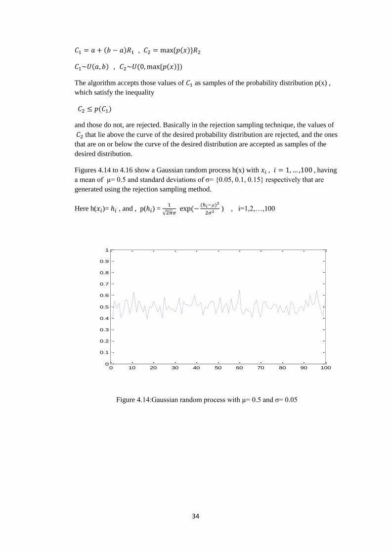
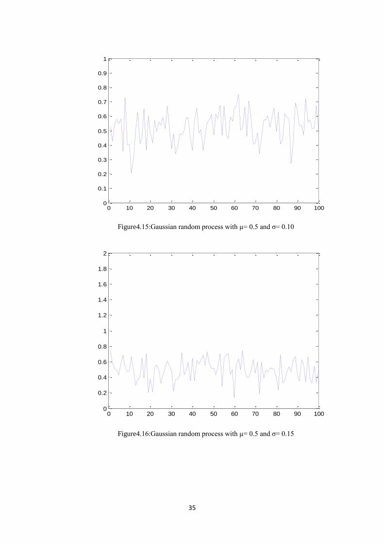
Figures 4.14 to 4.16 show a Gaussian random process h(x) with having
a mean of = 0.5 and standard deviations of = {0.05, 0.1, 0.15} respectively that are
generated using the rejection sampling method.
Here h( )= , and , p( ) =
√ (
( )
) , i=1,2,…,100
Figure 4.14:Gaussian random process with = 0.5 and = 0.05
0 10 20 30 40 50 60 70 80 90 1000
0.1
0.2
0.3
0.4
0.5
0.6
0.7
0.8
0.9
1
35
Figure4.15:Gaussian random process with = 0.5 and = 0.10
Figure4.16:Gaussian random process with = 0.5 and = 0.15
0 10 20 30 40 50 60 70 80 90 1000
0.1
0.2
0.3
0.4
0.5
0.6
0.7
0.8
0.9
1
0 10 20 30 40 50 60 70 80 90 1000
0.2
0.4
0.6
0.8
1
1.2
1.4
1.6
1.8
2
36
A question that arises is how exactly does the generated sequence behaves like Gaussian?
We need to verify that the generated sequence has a Gaussian distribution. A basic and
accurate method for classifying the resulting distribution of the generated sequence h is to
group the samples according to their amplitudes. This is achieved by splitting the total
amplitude range into a number of subranges of amplitudes. A couple of examples are
shown below for different sequences with the following properties
N= Number of samples generated in the sequence
h = Amplitude of the samples in the sequence
Number of amplitude subranges
Sequence 1 : µ=0.5, =0.1, N=1000 , =10, h ~ [0.2,0.8]
Interval 1: 0.20 Number of samples=0
Interval 2: 0.26 Number of samples=0
Interval 3: 0.32 Number of samples=8
Interval 4: 0.38 Number of samples=66
Interval 5: 0.44 Number of samples=253
Interval 6: 0.50 Number of samples=335
Interval 7: 0.56 Number of samples=257
Interval 8: 0.62 Number of samples=74
Interval 9: 0.68 Number of samples=7
Interval 10: 0.74 Number of samples=0
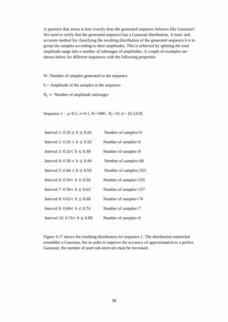
Figure 4.17 shows the resulting distribution for sequence 1. The distribution somewhat
resembles a Gaussian, but in order to improve the accuracy of approximation to a perfect
Gaussian, the number of used sub-intervals must be increased.
37
Figure4.17:The resulting distribution for sequence 1
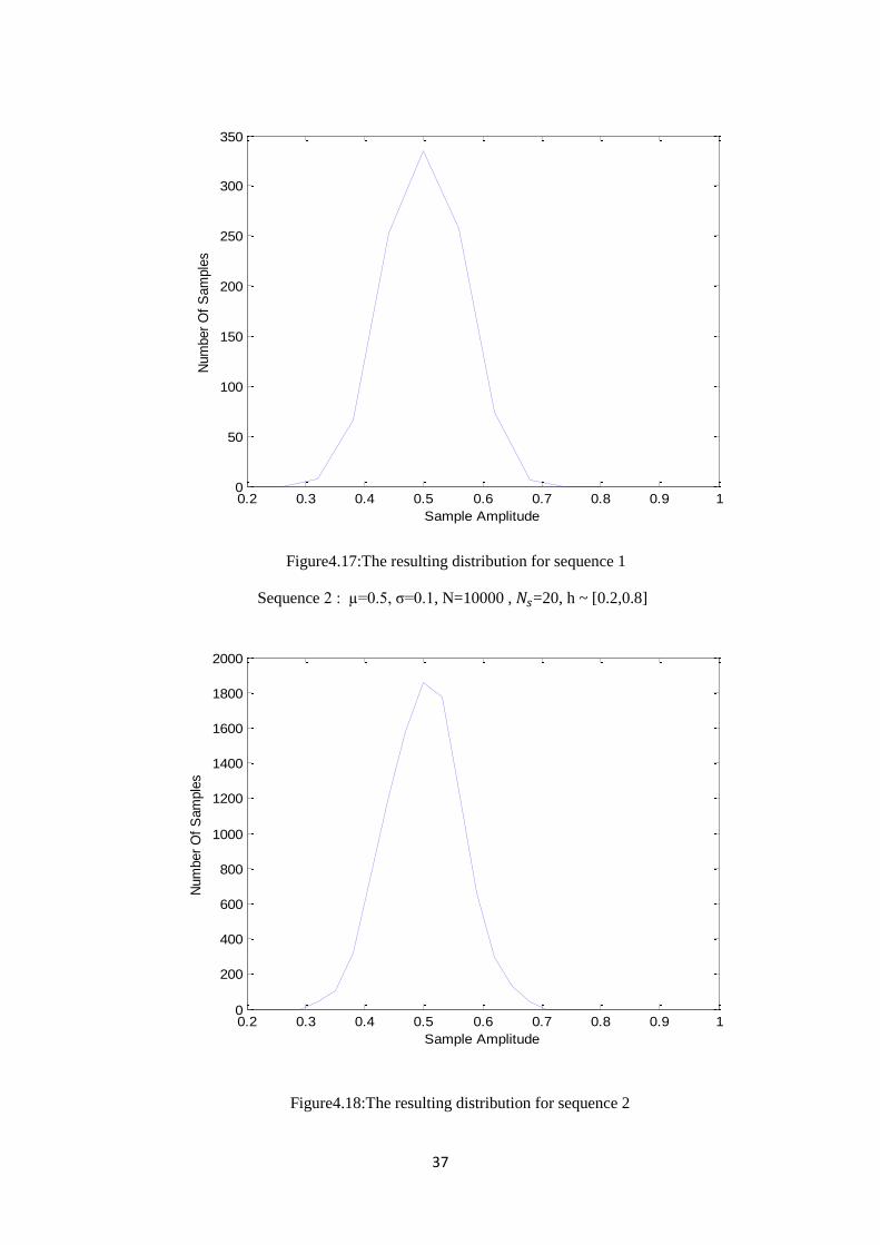
Sequence 2 : =0.5, =0.1, N=10000 , =20, h ~ [0.2,0.8]
Figure4.18:The resulting distribution for sequence 2
0.2 0.3 0.4 0.5 0.6 0.7 0.8 0.9 10
50
100
150
200
250
300
350
Sample Amplitude
Num
ber
Of
Sam
ple
s
0.2 0.3 0.4 0.5 0.6 0.7 0.8 0.9 10
200
400
600
800
1000
1200
1400
1600
1800
2000
Sample Amplitude
Num
ber
Of
Sam
ple
s
38
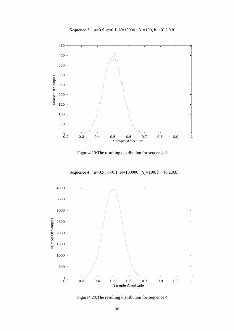
Sequence 3 : =0.5, =0.1, N=10000 , =100, h ~ [0.2,0.8]
Figure4.19:The resulting distribution for sequence 3
Sequence 4 : =0.5 , =0.1, N=100000 , =100, h ~ [0.2,0.8]
Figure4.20:The resulting distribution for sequence 4
0.2 0.3 0.4 0.5 0.6 0.7 0.8 0.9 10
50
100
150
200
250
300
350
400
450
Sample Amplitude
Num
ber
Of
Sam
ple
s
0.2 0.3 0.4 0.5 0.6 0.7 0.8 0.9 10
500
1000
1500
2000
2500
3000
3500
4000
Sample Amplitude
Num
ber
Of
Sam
ple
s
39
4.5 Mesh generation for analyzing rough surface scattering problem
If we are analyzing a rough surface scattering problem, we should be careful when
triangulating the region around the rough surface. Rough surface scattering problems can
be analyzed in regions with a rectangular outer PML boundary. Therefore the previously
described automatic mesh generation algorithm for rectangular domains can be used to
triangulate the solution region, except the region near the rough surface since the rough
surface has an irregular curvature due to its statistical property of having a Gaussian
distribution with a certain mean and standard deviation. That is why we need a seperate
triangulation around the rough surface and the rest of the solution region can be
triangulated identically the same as the previous description of automatic mesh generation
for rectangular regions. In order to seperate the two regions as the region around the rough
surface and the rectangular solution region which is the complement of the region around
the rough surface to the overall solution region, we call the region around the rough surface
as the “near-surface” region and the remaining part as the “complement region” and we use
an upper limit for the upper boundary of the near-surface region which is determined
according to the mean and the standard deviation value of the rough surface height.
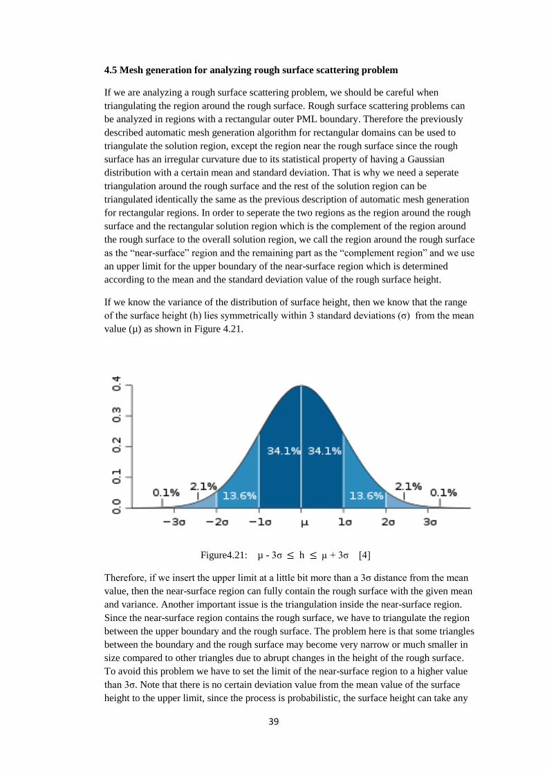
If we know the variance of the distribution of surface height, then we know that the range
of the surface height (h) lies symmetrically within 3 standard deviations ( ) from the mean
value (µ) as shown in Figure 4.21.
Figure4.21: µ - 3 h + 3 [4]
Therefore, if we insert the upper limit at a little bit more than a 3 distance from the mean
value, then the near-surface region can fully contain the rough surface with the given mean
and variance. Another important issue is the triangulation inside the near-surface region.
Since the near-surface region contains the rough surface, we have to triangulate the region
between the upper boundary and the rough surface. The problem here is that some triangles
between the boundary and the rough surface may become very narrow or much smaller in
size compared to other triangles due to abrupt changes in the height of the rough surface.
To avoid this problem we have to set the limit of the near-surface region to a higher value
than 3 . Note that there is no certain deviation value from the mean value of the surface
height to the upper limit, since the process is probabilistic, the surface height can take any
40
value. However the probability that the surface height may exceed a deviation of 3 from
the mean value is very small, therefore inserting the limit to a distance that is greater than
3 will usually result in more accurate triangulation with a lower probability of turning out
ill conditioned results. As we increase the limit from 3 to higher values we get better
results and the probability of getting ill conditioned results becomes smaller.
The overall solution region is terminated with an artificial absorbing medium that is called
“ PML” and is commonly used as an absorbing boundary condition in scattering or
radiation problems to limit the use of computer memory to a specified amount and to
effectively simulate the solution region to infinity by minimizing reflections from the outer
boundary. PML was discussed in detail in its own section in the previous chapter, but here
it is enough to know that PML surrounds the computational (solution) region and has a
specified thickness required for termination of the solution region in order to be used as an
artificial boundary. The thickness of the PML depends on the electrical characteristics of
the impinging wave and the solution region of interest.
The PML is a lossy medium which attenuates the incident wave with a rate that depends on
the conductivity value of the medium as described by Berenger [2]. Usually the attenuation
of the incident wave is very rapid. Therefore we should use smaller triangles with narrower
widths when discretizing the PML medium to handle rapid changes and to yield accurate
results. The size of the total mesh depends on the size of the solution region that we have
determined to analyze the scattering or radiation problem at hand and also the size of the
PML region necessary for terminating the solution region in order to minimize reflections.
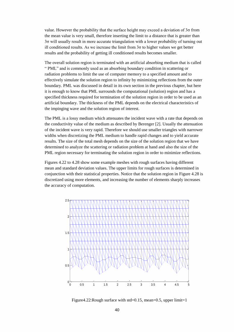
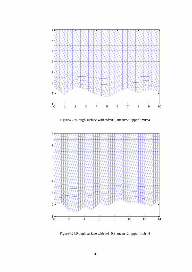
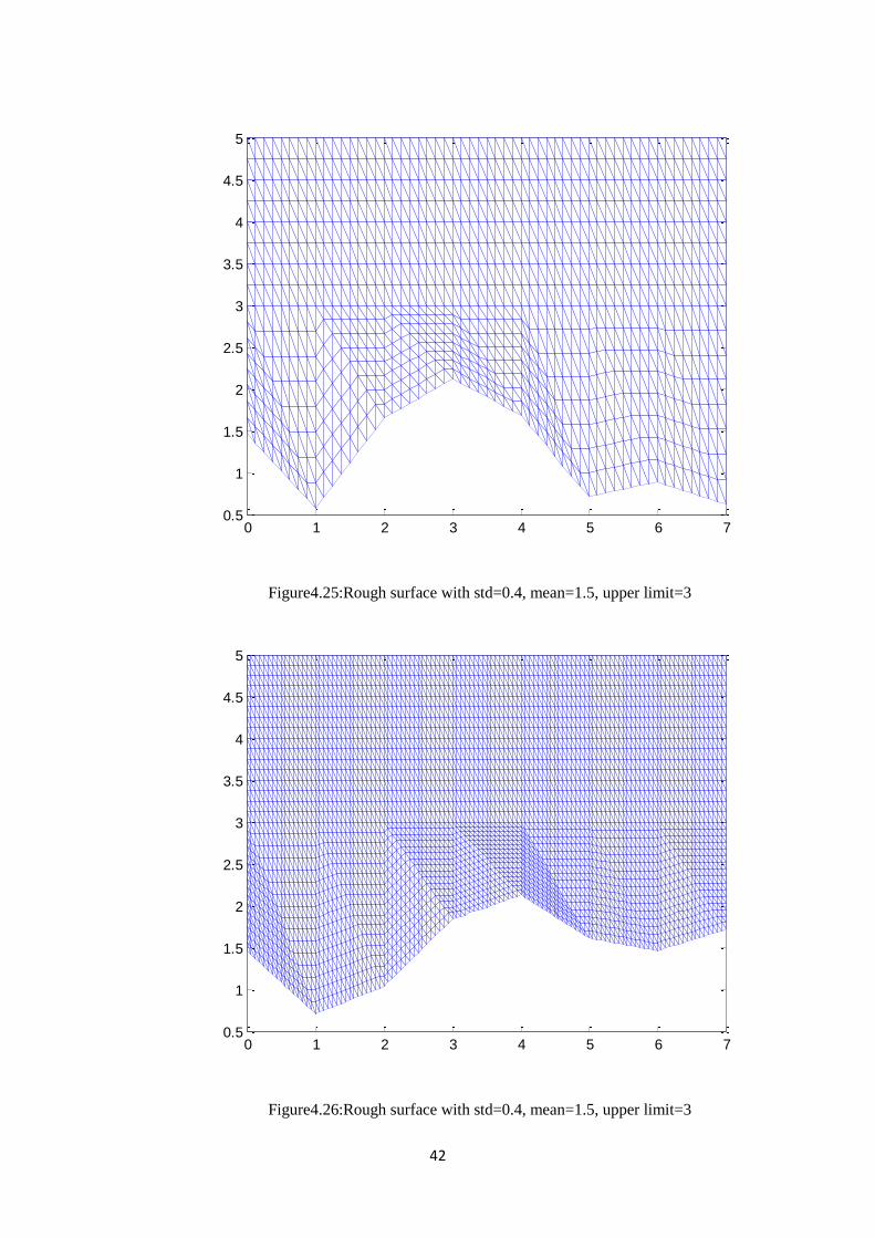
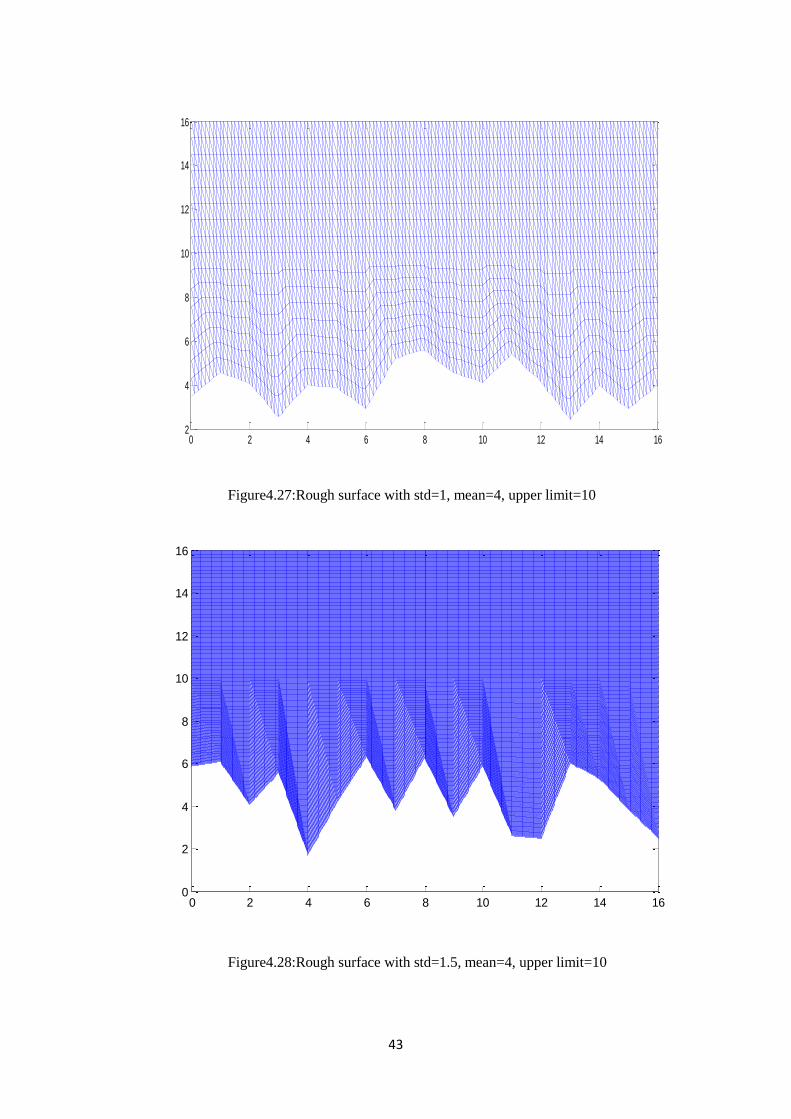
Figures 4.22 to 4.28 show some example meshes with rough surfaces having different
mean and standard deviation values. The upper limits for rough surfaces is determined in
conjunction with their statistical properties. Notice that the solution region in Figure 4.28 is
discretized using more elements, and increasing the number of elements sharply increases
the accuracy of computation.
Figure4.22:Rough surface with std=0.15, mean=0.5, upper limit=1
0 0.5 1 1.5 2 2.5 3 3.5 4 4.5 50
0.5
1
1.5
2
2.5
41
Figure4.23:Rough surface with std=0.5, mean=2, upper limit=4
Figure4.24:Rough surface with std=0.3, mean=2, upper limit=4
0 1 2 3 4 5 6 7 8 9 101
2
3
4
5
6
7
8
0 2 4 6 8 10 12 141
2
3
4
5
6
7
8
42
Figure4.25:Rough surface with std=0.4, mean=1.5, upper limit=3
Figure4.26:Rough surface with std=0.4, mean=1.5, upper limit=3
0 1 2 3 4 5 6 70.5
1
1.5
2
2.5
3
3.5
4
4.5
5
0 1 2 3 4 5 6 70.5
1
1.5
2
2.5
3
3.5
4
4.5
5
43
Figure4.27:Rough surface with std=1, mean=4, upper limit=10
Figure4.28:Rough surface with std=1.5, mean=4, upper limit=10
0 2 4 6 8 10 12 14 162
4
6
8
10
12
14
16
0 2 4 6 8 10 12 14 160
2
4
6
8
10
12
14
16
44
CHAPTER 5
BASICS OF THE TWO DIMENSIONAL FINITE ELEMENT METHOD
In order to use the finite element method for solving a partial differential equation (PDE) ,
we first have to convert the PDE of interest into its functional or variational form. To
convert a PDE into its functional form, we use the theory of calculus of variations which
focuses on the theory of extreme values of functionals. A functional is obtained by an
operator that operates on a function that is composed of one or more functions within
certain limits. Given the values of the independent variables to determine the output of the
function inside the operator, the output of a functional is a number which depends on the
form of the function inside the operator, and the form of the operator as well. The output of
a function depends only on the values of the independent variables.
Here we will deal with integral operators with certain limits that operate on a function. Our
aim is to determine the extreme values of the functional and the function that yields these
extreme values. The following discussion, up to section 5.3, is mostly referenced from [5].
Consider the functional ( ) given below
( ) ∫ (
)
Here is the independent variable and ( ) is a function of . Our goal is to find a
function ( ) that extremizes the functional ( ) along with the boundary conditions
( ) ( )
The integrand ( ) is a function with the independent variable , the dependent
variable and its derivative . Here ( ) is called a functional, or variational to be
extremized.
The variational operator δ is used to calculate the variation of a given function. In our
example, the variation δ of the function ( ) is the infinitesimal change in for a fixed
value of where δ =0. The variation of vanishes at points where is prescribed,
since the prescribed value can not be varied, and it can take any value at points where it is
not prescribed.
Since the integrand ( ) is a function of , a change in as δ will result in a change
in which is . Recalling the total differential of which is
We can write the first variation of at as
45
We know that since does not change as changes to , becomes
If the functional depends on second or higher order derivatives as shown
( ) ∫ (
( ))
Then the total differential and the first variational of are respectively
( ) ( )
( ) ( )
Thus the variational operator behaves like the differential operator.
If = ( ) and = ( ) , then the properties of the variational operator are as follows
( ) ( )
( ) ( )
( ) (
)
( ) ( ) ( )
( )
( )
( ) (
)
( ) ∫ ( ) ∫ ( )
For the functional ( ) to have an extremum, its variational must be zero , =0. This is
the starting condition for converting PDE s into their functional forms since this necessary
condition on the functional is usually in the form of a differential equation with boundary
conditions on the required function.
5.1 Converting PDEs into their functional forms
Given a partial differential equation, we can obtain its functional form using the following
procedure
1) Multiply the partial differential equation with the variational of the parameter of interest,
and integrate over the solution region.
46
2) Use integration by parts to express the derivatives in terms of the variational term.
3) Apply the boundary conditions to the resulting equation and bring the variational
operator outside the integral.
Let us start with a simple example of converting an ordinary differential equation into its
functional form. Consider the differential equation
Let us determine the functional for this ordinary differential equation subject to the
boundary conditions ( ) ( )
Then
∫ (
)
( )
∫
∫ ∫
Using integration by parts to express the derivatives inside the variational operator, the first
term becomes
∫
]
∫
(
)
therefore becomes
]
∫
∫
∫
Since a prescribed value can not be varied ( ) ( ) . Therefore the first term
vanishes , , using the properties of the variational operator δ , becomes
∫
(
) ∫
∫
∫ [ (
)
]
( )
∫ [
]
is the corresponding functional for the given differential equation.
Our interest here is to solve the inhomogenous wave equation using finite element method,
so we must determine the functional form of the inhomogenous wave equation
47
which will be solved by applying the finite element method to the functional form of the
equation, assuming that we are solving the equation in a 2 dimensional region. Using the
previously described procedure we will convert this PDE to its functional form as follows
∬[ ] δ
∬[ ] δ ∬[ ] δ ∬[ ] δ
The first term can be integrated using integration by parts, expanding the first term as
∬[ ] δ ∬[
] δ ∬[
] δ
and applying integration by parts by choosing
(
)
∫[∫
(
) ] ∫[
∫
]
∬[
δ ] ∫
∫
The single integrals become zero, if the boundary conditions are of the homogenous
Dirichlet or Neumann type. As a result, for most of the radiation/scattering problems we
have
∬[
δ ]
∬[ (
) (
) ]
( )
∬[ (
) (
) ]
is the corresponding functional for the inhomogenous wave equation.
The functional forms of the PDEs that are used in electromagnetics are given below for a 2
dimensional solution region. Since we have determined the functional form of the
inhomogenous wave equation, the functional forms of the other PDEs can be directly found
by simplification.
48
( )
∬[ (
) (
) ]
( )
∬[ (
) (
) ]
( )
∬[ (
)
(
)
]
( )
∬[ (
)
(
)
]
( ) for inhomogenous wave equation can also be determined using Mikhlin’s approach to
solve the equation
( )
where [ ] [ ] is the operator of the equation.
Other methods for deriving variational principles to solve electromagnetic problems also
exist in literature.
49
5.2 Solution of the Laplace equation using finite element method
We have already derived the functional for the inhomogenous wave equation
for a 2 dimensional solution region which is
( )
∬[ (
) (
) ]
Choosing , we get the functional for Laplace’s equation as
( )
∬[ (
)
(
)
]
Laplace's equation describes electrostatic problems with . To apply the
finite element method to solve Laplace's equation in a 2 dimensional region, we need to
follow the following procedure
1) Divide the solution region into finite elements, which are usually chosen as triangles.
2) Determine the interpolation functions (or shape functions) for each element in the
solution region.
3)Assemble all elements inside the solution region to get the resulting system of equations,
which is when solved, yields the approximate solution vector that we are looking for.
For a 2 dimensional solution region, we use either triangles or quadrilaterals to discretize
the solution region, since triangles fit better to curved boundaries we prefer to discretize
using triangles. After we decide which element type to use for discretization, we must
derive the representing equations for each element in the solution region. In other words we
need to determine the interpolation functions for each element. After determining the
interpolation functions for each element in the solution region, we use the three node
potential values (or field values) to determine a potential distribution function for each
element. Combining the potential distributions of all elements in the solution region, we get
the overall potential distribution of the solution region.
Figure 5.1 shows two solution regions, the one in the left being nonrectangular and other
being rectangular. The nonrectangular solution region is discretized using both triangles
and quadrilaterals, the rectangular one is discretized by using triangles only. Note that
there is always an unavoidable discretization error for nonrectangular solution regions.
50
Figure5.1:Discretization of rectangular and nonrectangular geometries.
If we know the potential distribution inside each element, which is (x,y), then the
approximate solution for the total region becomes
( ) ∑ ( )
where N is the total number of elements used inside the solution region.
(x,y) which is the potential distribution inside each element can be assumed to be in
polynomial form as, ( ) , then for a given element with vertices
{( ) ( ) ( ) , we have
[
] [
] [ ]
[ ] [
]
[
]
Using this equation along with the polynomial approximation ( ) , if
we express the potential inside an element in terms of the basis functions as
( ) ∑ ( )
51
Then we get as
[( ) ( ) ( ) ]
[( ) ( ) ( ) ]
[( ) ( ) ( ) ]
where A is the area of the element with coordinates {( ) ( ) ( ) , and can
be found from
[ ( )( ) ( )( ) ].
The value of the area is positive for counterclockwise numbering of the nodes, otherwise it
is negative.
Using the equation
( ) ∑ ( )
we can find the potential value anywhere inside an element, i.e., potential distribution is
continuous unlike in the case of finite difference method where the potential values are
known only at the grid points.
Element shape functions have the following two properties
{
∑
( )
For example, an element with vertices
( ) ( ) ( ) ( ) ( ) ( ) , has
[( ) ( ) ( ) ]
[( ) ( ) ( ) ]
[( ) ( ) ( ) ]
with potential values at the three vertices as , , the potential
distribution inside the triangle is determined by the function
( ) ∑ ( )
52
In order to solve Laplace’s equation, which has the functional
( )
∬[ ]
∫[ ]
in a two dimensional solution region, we use the energy functional given by
∫
∫
where is the energy per unit length. For a single element e , becomes , which is
the energy per unit length inside an element e, given by
∫
∫
We have defined , the potential distribution inside an element e as
∑
( )
Therefore the gradient of the expression is
∑
( )
Substituting this equation into the expression for , we get
∑∑
Which is when substituted into the equation for , yields
∫ [ ∑∑
]
Moving the sums, along with and , out of the integral, we get
∑∑ [∫
]
The term inside the brackets is defined as the {i,j} th entry of the element coefficient
matrix [ ( )] , that is defined as
( ) ∫
53
Therefore
∑∑
( )
which can be written in matrix form as (with denoting transposition)
[ ]
[ ( )] [ ] [ ] [
]
[ ( )] [
( )
( ) ( )
( )
( ) ( )
( )
( ) ( )
]
Since
( ) ∫ ∫
( )
The element coefficient matrix [ ( )] is symmetric.
With and already known, we can directly determine ( ) , , as
( )
[ ]
( ) ( ) ( )
( ) ( ) ( )
[ ]
[ ( )] [ ] , is defined for a single element. To get the total energy per unit
length inside the overall solution region, we sum the energies of all elements in the region
∑
[ ] [ ] [ ]
[
]
Where is the number of elements and is the number of nodes in the solution region.
[ ] is called the global coefficient matrix that is assembled using the individual element
coefficient matrices, according to their connections.
can be expanded from its matrix equation form to its general equation form as
[ ] [
]
[
]
54
[
]
[
]
[
]
It can be shown that Laplace’s equation is satisfied, when becomes minimum at all
nodes inside the solution region, therefore we require
By satisfying the condition
, at every node in the solution
region we get a system of linear equations
So in general
yields
∑
∑
Which has a solution for an arbitrary free node , given as
∑
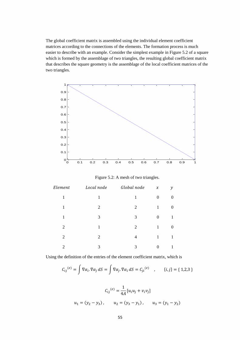
55
The global coefficient matrix is assembled using the individual element coefficient
matrices according to the connections of the elements. The formation process is much
easier to describe with an example. Consider the simplest example in Figure 5.2 of a square
which is formed by the assemblage of two triangles, the resulting global coefficient matrix
that describes the square geometry is the assemblage of the local coefficient matrices of the
two triangles.
Figure 5.2: A mesh of two triangles.
1 1 1 0 0
1 2 2 1 0
1 3 3 0 1
2 1 2 1 0
2 2 4 1 1
2 3 3 0 1
Using the definition of the entries of the element coefficient matrix, which is
( ) ∫ ∫
( )
( )
[ ]
( ) ( ) ( )
0 0.1 0.2 0.3 0.4 0.5 0.6 0.7 0.8 0.9 10
0.1
0.2
0.3
0.4
0.5
0.6
0.7
0.8
0.9
1
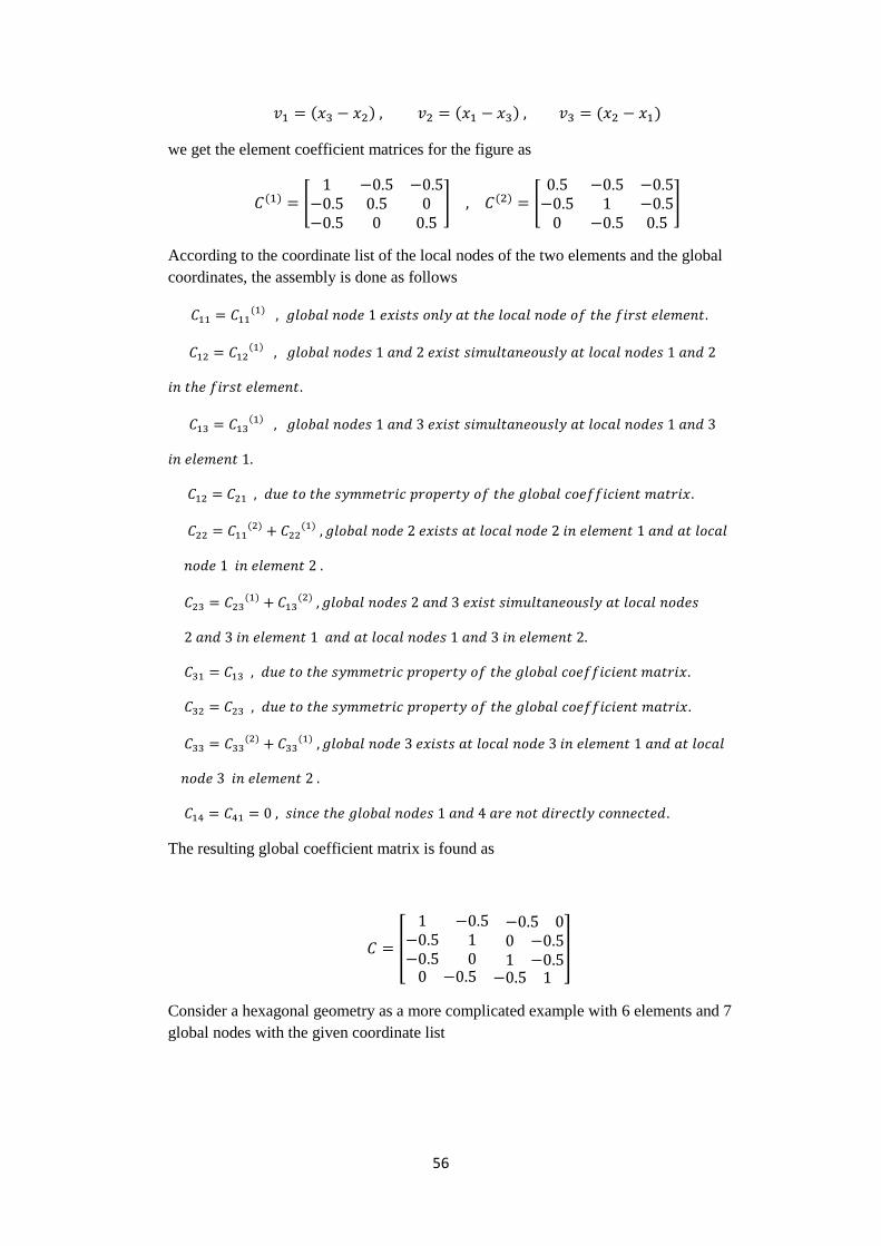
56
( ) ( ) ( )
we get the element coefficient matrices for the figure as
( ) [
] ( ) [
]
According to the coordinate list of the local nodes of the two elements and the global
coordinates, the assembly is done as follows
( )
( )
( )
( )
( )
( )
( )
( )
( )
The resulting global coefficient matrix is found as
[
]
Consider a hexagonal geometry as a more complicated example with 6 elements and 7
global nodes with the given coordinate list
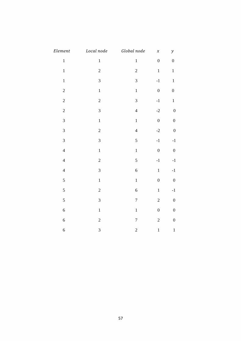
57
1 1 1 0 0
1 2 2 1 1
1 3 3 -1 1
2 1 1 0 0
2 2 3 -1 1
2 3 4 -2 0
3 1 1 0 0
3 2 4 -2 0
3 3 5 -1 -1
4 1 1 0 0
4 2 5 -1 -1
4 3 6 1 -1
5 1 1 0 0
5 2 6 1 -1
5 3 7 2 0
6 1 1 0 0
6 2 7 2 0
6 3 2 1 1
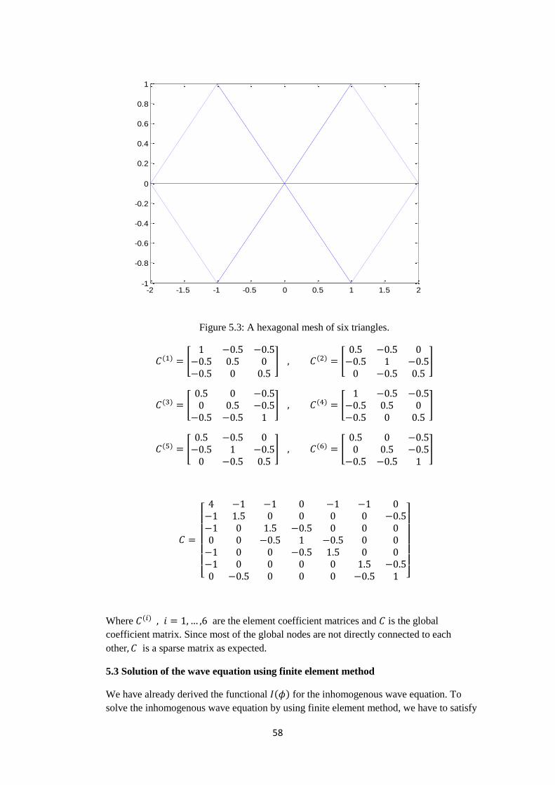
58
Figure 5.3: A hexagonal mesh of six triangles.
( ) [
] ( ) [
]
( ) [
] ( ) [
]
( ) [
] ( ) [
]
[ ]
Where ( ) are the element coefficient matrices and is the global
coefficient matrix. Since most of the global nodes are not directly connected to each
other is a sparse matrix as expected.
5.3 Solution of the wave equation using finite element method
We have already derived the functional ( ) for the inhomogenous wave equation. To
solve the inhomogenous wave equation by using finite element method, we have to satisfy
-2 -1.5 -1 -0.5 0 0.5 1 1.5 2-1
-0.8
-0.6
-0.4
-0.2
0
0.2
0.4
0.6
0.8
1
59
the given boundary conditions and we have to minimize the functional ( ) at each free
node inside the solution region. Again, first we need to express ( ) in terms of the global
coefficient matrix to obtain a matrix equation form of ( ). We will follow an identical
procedure as we did for Laplace’s equation. Recall that the inhomogenous wave equation
is expressed in its functional form as
( )
∬[ (
) (
) ]
∬[ ]
Our aim is to determine the unknown at every free node inside the solution region. The
wave equation is inhomogenous, thus a prescribed source function also exists in the
solution region. We start by expressing in terms of the element shape functions
( ) ∑ ( )
( ) ∑ ( )
Where and are the values of and at node in element .
Substituting the expressions for and into ( ) , we get ( ) as
( )
∑∑ ∫∫(
)
∑∑ ∫∫(
)
∑∑ ∫∫(
)
Where the element coefficient matrices are defined as
( ) ∫∫
( ) ∫∫
( ) ∫∫ {
In matrix form, we can write ( ) as
( )
[ ]
[ ( )] [ ]
[ ]
[ ( )] [ ] [ ] [ ( )] [ ]
where [ ] [ ] , [ ] [ ]
60
( ) is defined for a single element. To determine ( ) which is defined for the
assemblage of all elements, we sum the functionals ( ) , of each
element in the solution region , so that ( ) becomes
( ) ∑ ( )
[ ] [ ] [ ]
[ ] [ ] [ ] [ ] [ ] [ ]
[ ] [ ] , [ ] [ ]
Where [C] and [T] are global coefficient matrices.
We can expand the matrix equation for ( ) into its algebraic form and then minimize
( ) at every free node in the solution region. To do this we split ( ) into three parts as
described below
( ) ( ) ( ) ( )
[ ] [ ] [ ]
[ ] [ ] [ ] [ ] [ ] [ ]
( )
[ ] [ ] [ ] ( )
[ ] [ ] [ ] ( ) [ ] [ ] [ ]
( )
[ (
)
( ) (
) + … + (
) ]
( )
[ (
)
( ) (
) + … + (
) ]
( ) [ ( ) (
) ( ) + … + (
) ]
61
We are trying to determine the vector [ ] [ ] which satisfies ( )
at all free nodes So we need to determine the expression
for ( )
, . The process is as described below
( )
( )
( )
( )
( )
( )
( )
( )
Therefore, in general, we have
( )
∑
Similarly
( )
[ ]
( )
[ ]
( )
[ ]
( )
[ ]
( )
[ ] ∑
( ) contains the source term therefore
( )
[ ]
62
( )
[ ]
( )
[ ]
In general
( )
∑
[ ]
Therefore , ( )
( )
( )
( )
= 0, is expressed as
( )
∑
∑
∑
( )
∑
( )
∑ [
]
If there are no sources in the solution region then the equation simplifies to
( )
∑ [
]
Equations are given for a homogenous medium with a constant value of the wavenumber
which is determined from the constitutive parameters of the medium. If the medium is a
homogenous, isotropic, and lossless , is given as
√
As we increase the mesh size and the number of elements used, the resolution also
increases and we get better simulation results. However this greatly increases the required
computation time of the problem. In order to find the solution of the wave equation in a
given solution region with the specified boundary conditions, first, the computer assigns
global node numbers to the coordinates of each node inside the mesh, then it determines the
element coefficient matrices of each element in the solution region and finally it assembles
all element coefficient matrices. Especially the assembling process requires a great amount
of computation time. Therefore when simulating the solution of a partial differential
equation in a given solution region, a huge trade-off exists between resolution and
computation time.
When the medium is not homogenous, or when the wavenumber, k, is not a constant but an
element varying quantity, we have to introduce a different element coefficient matrix that
takes the variation of ‘k’ from one element to another, into account. For an element varying
wavenumber ‘k’ the functional ( ) becomes
63
( )
∑∑ ∫∫(
)
∑∑
∫∫(
)
∑∑ ∫∫(
)
( ) ∫∫
( ) ∫∫
( )
∑∑ [ ∫∫( )
∫∫( ) ]
∑∑ ∫∫(
)
Here, we can introduce the coefficient matrix ( ) , which is defined as
( )
( )
( )
( ) [ ∫∫( )
∫∫( ) ]
Therefore ( ) can be written as
( )
∑∑
( ) ∑∑
( )
( )
∑∑
[ ( )
( )]
( ) , for element varying ‘k’ , can be written in matrix form as
( )
[ ]
[ ( )] [ ] [ ] [ ( )] [ ]
Summing ( ) for all elements in the solution region, we get
( ) ∑ ( )
( )
[ ] [ ] [ ] [ ] [ ] [ ]
[ ] [ ] , [ ] [ ]
64
Where [M] and [T] are global coefficient matrices. [M] and [T] are assembled using the
previously described procedure in which we have assembled [C].
( ) ( ) ( )
( )
[ ] [ ] [ ] ( ) [ ] [ ] [ ]
Following the same procedure as before, we have
( )
( )
( )
( )
∑
( )
∑
[ ]
Therefore, we have
( )
∑
∑
∑
If there are no sources in the solution region
∑
Using the last two identities , , i=1,2,…,n , can be easily solved. In this procedure we
have treated the wavenumber ‘k’ as an element variable instead of a global node variable,
but at the same time we have treated the source ‘g’ as a node variable. We can also assume
that ‘g’ is an element variable along with ‘k’ , but then we would have to define another
element coefficient matrix regarding the source ‘g’, this is the easiest approach for
computation.
As the final case, consider that both and are element variables, in that case ( )
becomes
( )
∑∑ [ ∫∫( )
∫∫( ) ]
∑∑ ∫∫(
)
65
Therefore ( ) can be written as
( )
∑∑
( ) ∑∑
( )
Since ( ) is symmetric, i.e ,
( ) ( ) , we can also write
( )
∑∑
( ) ∑∑
( )
This equation can be written in matrix form as
( )
[ ]
[ ( )] [ ] [ ] [ ( )]
In order for ( ) to be a scalar quantity , [ ] [ ( )] , must also be scalar, which
dictates that the element coefficient matrix [ ( )] must actually be a [3x1] vector.
Therefore, concerning , we have an element coefficient vector ( ) [ ( )]
which is
( ) [
( )
( ) ( )
( )
( ) ( )
( )
( ) ( )
] ( ) [
( )
( ) ( )
( )
( ) ( )
( )
( ) ( )
]
Therefore
( )
[ ]
[ ( )] [ ] [ ] [ ( )]
Summing ( ) for all elements in the solution region
( ) ∑ ( )
( )
[ ] [ ] [ ] [ ] [ ]
( )
Which yields to
( )
∑[
]
∑
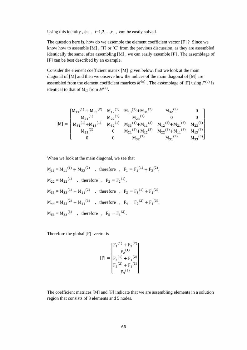
66
Using this identity , , i=1,2,…,n , can be easily solved.
The question here is, how do we assemble the element coefficient vector [F] ? Since we
know how to assemble [M] , [T] or [C] from the previous discussion, as they are assembled
identically the same, after assembling [M] , we can easily assemble [F] . The assemblage of
[F] can be best described by an example.
Consider the element coefficient matrix [M] given below, first we look at the main
diagonal of [M] and then we observe how the indices of the main diagonal of [M] are
assembled from the element coefficient matrices ( ) . The assemblage of [F] using ( ) is
identical to that of from ( )
[ ]
[
( ) ( )
( ) ( )
( ) ( )
( )
( ) ( )
( )
( ) ( )
( ) ( )
( ) ( )
( )
( )
( ) ( )
( ) ( )
( )
( )
( ) ( )]
When we look at the main diagonal, we see that
= ( )
( ) , therefore , ( )
( ).
= ( ) , therefore ,
( ).
= ( )
( ) , therefore , ( )
( ).
= ( )
( ) , therefore , ( )
( ).
= ( ) , therefore ,
( ).
Therefore the global [F] vector is
[ ]
[
( ) ( )
( )
( )
( )
( )
( )
( ) ]
The coefficient matrices [M] and [F] indicate that we are assembling elements in a solution
region that consists of 3 elements and 5 nodes.
67
Note that the symmetry property of the element coefficient matrices and the global
coefficient matrices provides speed for computation, since we only have to calculate the
upper triangular part of the matrices.
5.4 Prescribed and free nodes of a solution region
In order to evaluate the solution at all nodes inside a given region, we need to know the
solution at the boundary of the given region. The nodes at the boundary are known as the
prescribed nodes of the solution region where the solution is already known or prescribed.
For the solution of Helmholtz equation or phasor domain wave equation, the values of
prescribed nodes at the boundary of the solution region can be determined using the
incident or incoming wave that impinges on the boundary of the solution region. Using the
general boundary conditions described in chapter 2, the prescribed node values can be
determined directly from the incident field if the wave equation contains no source term, i.e
g=0. But if the source term is not zero, the prescribed node values can be determined using
the boundary conditions that occur when there are sources at the boundary between two
different media (see chapter 2).
Consider the FEM (Finite Element Method) solution of a 2D homogenous wave equation.
The FEM solution to this problem can be obtained by solving the system linear of
equations generated by the previously found formula
( )
∑ [
] √
[ ] [ ] [ ]
[ ] [ ] [ ]
[ ] [ ] [ ]
[ ] [ ] [ ]
•
•
•
[ ] [ ] [ ]
( )
∑ [
] √
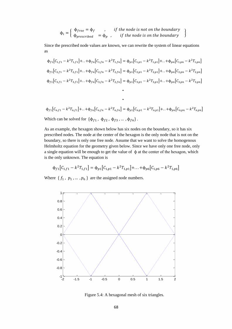
68
{
}
Since the prescribed node values are known, we can rewrite the system of linear equations
as
[ ] [ ] [ ] [ ]
[ ] [ ] [ ] [ ]
[ ] [ ] [ ] [ ]
•
•
[ ] [ ] [ ] [ ]
Which can be solved for .
As an example, the hexagon shown below has six nodes on the boundary, so it has six
prescribed nodes. The node at the center of the hexagon is the only node that is not on the
boundary, so there is only one free node. Assume that we want to solve the homogenous
Helmholtz equation for the geometry given below. Since we have only one free node, only
a single equation will be enough to get the value of ф at the center of the hexagon, which
is the only unknown. The equation is
[ ] [ ] [ ]
Where are the assigned node numbers.
Figure 5.4: A hexagonal mesh of six triangles.
-2 -1.5 -1 -0.5 0 0.5 1 1.5 2-1
-0.8
-0.6
-0.4
-0.2
0
0.2
0.4
0.6
0.8
1
69
5.5 Examples of 2D FEM solutions of the Helmholtz equation in a closed region
Consider the hexagon example given in the previous section. If the prescribed nodes at the
boundary are numbered as { and the free node at the center is
numbered as , we can solve for by using the linear system
( )
∑ [
] √
Since in that case there is only one free node, we need only one equation to solve
[ ] [ ] [ ]
[ ]
[ ]
[ ]
[ ]
[ ]
[ ]
( )
[ ]
( ) ( ) ( )
( ) ( ) ( )
( ) ∫∫ {
( )
( )
As another example, consider a triangular mesh with 15 nodes where 3 of the nodes are in
the interior region of the triangle and the others are at the boundary.
{
}
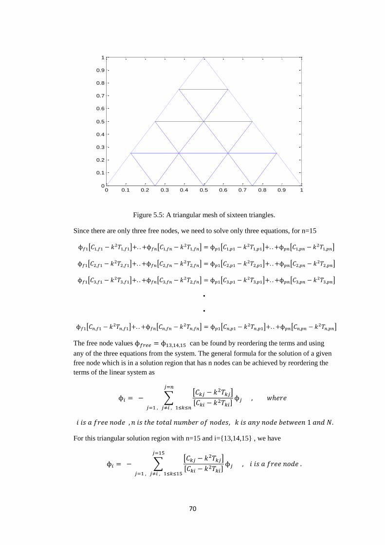
70
Figure 5.5: A triangular mesh of sixteen triangles.
Since there are only three free nodes, we need to solve only three equations, for n=15
[ ] [ ] [ ] [ ]
[ ] [ ] [ ] [ ]
[ ] [ ] [ ] [ ]
•
•
[ ] [ ] [ ] [ ]
The free node values can be found by reordering the terms and using
any of the three equations from the system. The general formula for the solution of a given
free node which is in a solution region that has n nodes can be achieved by reordering the
terms of the linear system as
∑[ ]
[ ]
For this triangular solution region with n=15 and i={13,14,15} , we have
∑[ ]
[ ]
0 0.1 0.2 0.3 0.4 0.5 0.6 0.7 0.8 0.9 10
0.1
0.2
0.3
0.4
0.5
0.6
0.7
0.8
0.9
1
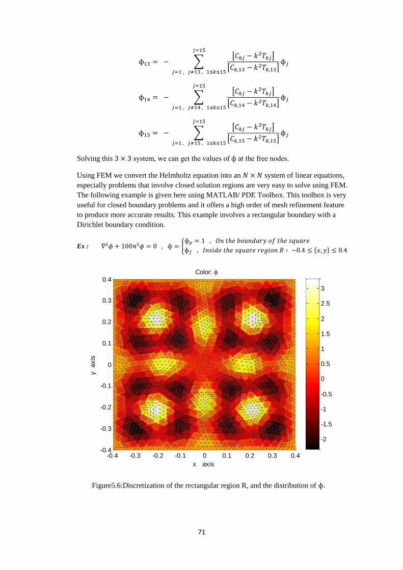
71
∑[ ]
[ ]
∑[ ]
[ ]
∑[ ]
[ ]
Solving this system, we can get the values of ф at the free nodes.
Using FEM we convert the Helmholtz equation into an system of linear equations,
especially problems that involve closed solution regions are very easy to solve using FEM.
The following example is given here using MATLAB/ PDE Toolbox. This toolbox is very
useful for closed boundary problems and it offers a high order of mesh refinement feature
to produce more accurate results. This example involves a rectangular boundary with a
Dirichlet boundary condition.
Ex : {
Figure5.6:Discretization of the rectangular region R, and the distribution of .
-0.4 -0.3 -0.2 -0.1 0 0.1 0.2 0.3 0.4-0.4
-0.3
-0.2
-0.1
0
0.1
0.2
0.3
0.4
x axis
Color:
y
axis
-2
-1.5
-1
-0.5
0
0.5
1
1.5
2
2.5
3
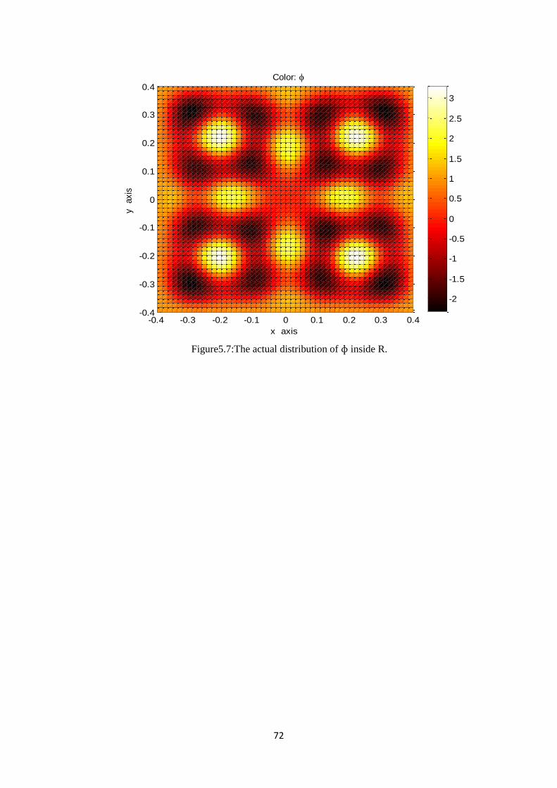
72
Figure5.7:The actual distribution of inside R.
-0.4 -0.3 -0.2 -0.1 0 0.1 0.2 0.3 0.4-0.4
-0.3
-0.2
-0.1
0
0.1
0.2
0.3
0.4
x axis
Color:
y
axis
-2
-1.5
-1
-0.5
0
0.5
1
1.5
2
2.5
3
73
CHAPTER 6
APPLICATION OF FEM ON ROUGH SURFACE SCATTERING PROBLEMS
We have previously described the conversion of the scalar wave equation in phasor form,
into a linear system of equations. After this conversion we discretize the solution region
using triangles and assemble the global coefficient matrix using the individual coefficient
matrices of each element in the region to solve the linear system. In order to solve the
linear system, we need prescribed values, which can be obtained by imposing the boundary
conditions at the surface boundary. Having the global coefficient matrix values and the
prescribed node values at hand, we can solve the linear system of equations to get the node
values everywhere inside the solution region.
Since we know the coordinates of each element in the solution region, assembling the
global coefficient matrix can be thought as the easy part. What is important is to impose the
surface boundary condition on the rough surface.
In electromagnetics, surfaces, whether flat or arbitrary in shape, indicate the sudden change
of constitutive parameters in an unbounded domain or space. Therefore a surface can be
dielectric, good conductor, weak conductor, or a perfect conductor. Depending on the
constitutive parameters of the surface an incident field produces a scattered field and a
transmitted field on the surface. Here, we want to obtain the scattered field as we are
interested in the domain where the incident field exists.
For perfect electric conductor (PEC) surfaces, the tangential component of the scattered
field is equal to the incident field in magnitude and there is a phase difference
between the two. Basically for a incident wave, we have
However, if the surface boundary is not a PEC, then we must use an impedance boundary
condition on the surface, one approach is to use Kirchoff’s approximation which
approximates each point on the surface with a tangent plane at that point and evaluates the
scattered field on that point as if the point is on a flat surface (tangential planar surface).
Another approach is to apply the impedance boundary condition embedded in the finite
element method itself by modifying the coefficient matrices of elements that are on the
surface. In this approach, element coefficient matrices of surface elements are modified to
include the loss effect of the surface, but the coefficient matrices of elements that are not
on the surface remain unchanged. In the end, all of the element coefficient matrices are
assembled to form the global coefficient matrix as before and using the incident field and
the surface loss factor we form the output result vector and solve the linear system. We will
use this latter approach and explain it in detail.
74
Electromagnetic scattering problems involve open boundaries, and open boundary problems
are more complicated compared to problems involving closed boundaries. When we are
dealing with open boundary problems, we have to limit our computational domain of interest
to a manageable size, otherwise the size of the computational region is infinite. This can be
achieved by applying grid truncation techniques known as Absorbing Boundary
Conditions(ABC). There are lots of ABC formulations in literature, the most commonly used
one is Berenger’s Perfectly Matched Layer (PML) [2], which suggests the use of an artificial
absorbing layer of material to realize the absorbing boundary condition. After the
introduction of an initial PML model by Berenger in 1994, the concept has been further
developed by many others. Modifications made on the initial concept of PML have led to
much more applicable and accurate PML realizations regarding the realization of absorbing
boundary conditions. One of them is the Locally Conformal Perfectly Matched Layer, which
uses a non-Maxwellian approach to impose an absorbing boundary condition and achieves
non-Maxwellian PML realization by using complex coordinate transformation. We will use
the locally conformal PML approach and explain it in some detail, more detailed information
about locally conformal PML can be found in the journal by Ozgun and Kuzuoglu[6].
Recall that the finite element method solution of a scalar 2D homogenous wave equation in
phasor domain can be determined for each node , from the linear system
( )
∑ [
] √
[ ] [ ] [ ]
[ ] [ ] [ ]
[ ] [ ] [ ]
[ ] [ ] [ ]
•
•
•
[ ] [ ] [ ]
{
}
75
Using the incident field and the appropriate boundary condition on a given rough surface,
we can get the field values of the rough surface nodes, which are called prescribed nodes
therefore we can rewrite the system in terms of free and prescribed nodes as
[ ] [ ] [ ] [ ]
[ ] [ ] [ ] [ ]
[ ] [ ] [ ] [ ]
•
•
[ ] [ ] [ ] [ ]
Which can be solved for .
However, since we are interested in an open boundary problem which is rough surface
scattering, we must first limit the size of the computational domain such that it will be
enough for us to observe the scattered field behaviour. Because, in order to solve a linear
system, we need to know the size of the linear system and the size of the linear system is
determined by the total number of nodes in the solution region. Using PML, we can limit our
solution region to a manageable size and only after we limit our solution region, we can get
the total number of nodes in our solution region. Therefore the first thing to do when dealing
with a scattering problem, is to limit the size of the domain in accordance with our solution
region of interest and the required computer memory. This is achieved by using PML as an
absorbing boundary condition. Due to its accuracy and ease of implementation, we will use
the Locally Conformal Perfectly Matched Layer as described in[6].
After the implementation of a locally conformal PML, we must determine the values of the
prescribed nodes using a surface impedance boundary condition over the rough surface.
Having determined the size of the computational domain and the values of the prescribed
nodes, we can solve the resulting linear system to get the node (field) values everywhere.
So, first we will limit the size of the computational domain using a locally conformal PML
and then we will impose an impedance boundary condition over a given rough surface.
Therefore we will now discuss these two topics respectively, before proceeding into the
solution of a rough surface scattering problem.
6.1 Locally-conformal perfectly matched layer
The perfectly matched layer (PML) is an artificial layer that is used to bound the
computational domain when we are dealing with an unbounded domain. A PML must
completely absorb the outgoing waves without yielding any reflections for any given
frequency and incidence angle. In other words a PML must be reflectionless to provide
accurate results.
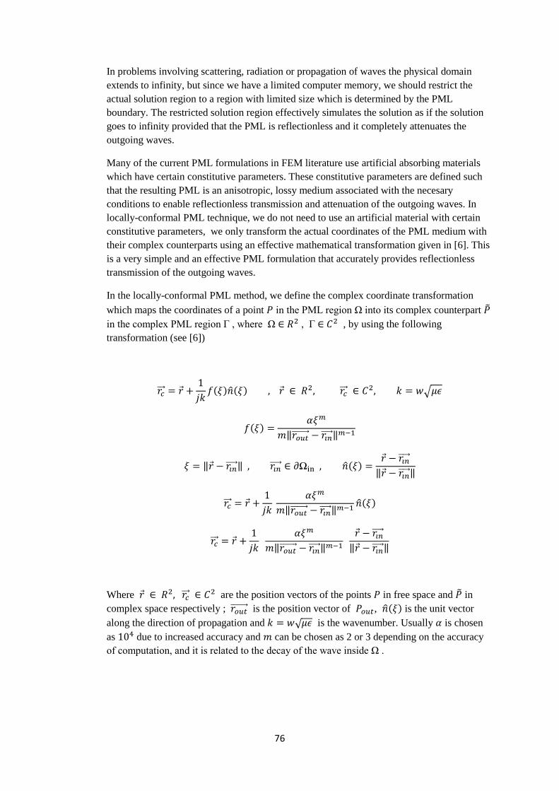
76
In problems involving scattering, radiation or propagation of waves the physical domain
extends to infinity, but since we have a limited computer memory, we should restrict the
actual solution region to a region with limited size which is determined by the PML
boundary. The restricted solution region effectively simulates the solution as if the solution
goes to infinity provided that the PML is reflectionless and it completely attenuates the
outgoing waves.
Many of the current PML formulations in FEM literature use artificial absorbing materials
which have certain constitutive parameters. These constitutive parameters are defined such
that the resulting PML is an anisotropic, lossy medium associated with the necesary
conditions to enable reflectionless transmission and attenuation of the outgoing waves. In
locally-conformal PML technique, we do not need to use an artificial material with certain
constitutive parameters, we only transform the actual coordinates of the PML medium with
their complex counterparts using an effective mathematical transformation given in [6]. This
is a very simple and an effective PML formulation that accurately provides reflectionless
transmission of the outgoing waves.
In the locally-conformal PML method, we define the complex coordinate transformation
which maps the coordinates of a point in the PML region Ω into its complex counterpart
in the complex PML region Γ , where Ω , Γ , by using the following
transformation (see [6])
( ) ( ) √
( )
‖ ‖
‖ ‖ ( )
‖ ‖
‖ ‖ ( )
‖ ‖
‖ ‖
Where are the position vectors of the points in free space and in
complex space respectively ; is the position vector of , ( ) is the unit vector
along the direction of propagation and √ is the wavenumber. Usually is chosen
as due to increased accuracy and can be chosen as 2 or 3 depending on the accuracy
of computation, and it is related to the decay of the wave inside Ω .
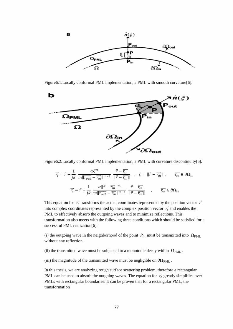
77
Figure6.1:Locally conformal PML implementation, a PML with smooth curvature[6].
Figure6.2:Locally conformal PML implementation, a PML with curvature discontinuity[6].
‖ ‖
‖ ‖ ‖ ‖
‖ ‖
‖ ‖
‖ ‖
This equation for transforms the actual coordinates represented by the position vector
into complex coordinates represented by the complex position vector and enables the
PML to effectively absorb the outgoing waves and to minimize reflections. This
transformation also meets with the following three conditions which should be satisfied for a
successful PML realization[6]:
(i) the outgoing wave in the neighborhood of the point must be transmitted into
without any reflection.
(ii) the transmitted wave must be subjected to a monotonic decay within .
(iii) the magnitude of the transmitted wave must be negligible on .
In this thesis, we are analyzing rough surface scattering problem, therefore a rectangular
PML can be used to absorb the outgoing waves. The equation for greatly simplifies over
PMLs with rectangular boundaries. It can be proven that for a rectangular PML, the
transformation
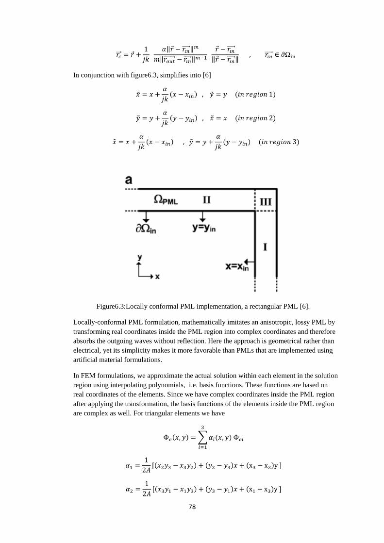
78
‖ ‖
‖ ‖
‖ ‖
In conjunction with figure6.3, simplifies into [6]
( ) ( )
( ) ( )
( )
( ) ( )
Figure6.3:Locally conformal PML implementation, a rectangular PML [6].
Locally-conformal PML formulation, mathematically imitates an anisotropic, lossy PML by
transforming real coordinates inside the PML region into complex coordinates and therefore
absorbs the outgoing waves without reflection. Here the approach is geometrical rather than
electrical, yet its simplicity makes it more favorable than PMLs that are implemented using
artificial material formulations.
In FEM formulations, we approximate the actual solution within each element in the solution
region using interpolating polynomials, i.e. basis functions. These functions are based on
real coordinates of the elements. Since we have complex coordinates inside the PML region
after applying the transformation, the basis functions of the elements inside the PML region
are complex as well. For triangular elements we have
( ) ∑ ( )
[( ) ( ) ( ) ]
[( ) ( ) ( ) ]
79
[( ) ( ) ( ) ]
If we consider region 3 in Figure6.3 as an example, after complex coordinate transformation,
the coordinates and the formulation become
( )
( )
[( ) ( ) ( ) ]
[( ) ( ) ( ) ]
[( ) ( ) ( ) ]
( ) ∑ ( )
After the transformation, we follow the previously described FEM procedure, here the
coordinates of the elements inside the PML region are complex, this will cause the
outgoing waves to decay gradually and efficiently and enables us to analyze scattering
problems accurately.
6.2.1 Imposing boundary conditions on the rough surface – Kirchoff’s approximation
The incident wave hits on the rough surface boundary and based on the constitutive
rough surface parameters, there will be a scattered field on the rough surface boundary. In
the case of an infinite and a perfectly flat boundary, the incident and reflected fields are
related with the which are given for
and polarizations as
( ) ( )
( ) ( )
( ) ( )
( ) ( )
( ) ( )
√ {
[√ (
) ] }
√ {
[√ (
) ] }
(
( ))
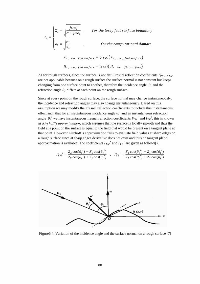
80
{
√
√
( )( )
( )( )
As for rough surfaces, since the surface is not flat, Fresnel reflection coefficients
are not applicable because on a rough surface the surface normal is not constant but keeps
changing from one surface point to another, therefore the incidence angle and the
refraction angle differs at each point on the rough surface.
Since at every point on the rough surface, the surface normal may change instantaneously,
the incidence and refraction angles may also change instantaneously. Based on this
assumption we may modify the Fresnel reflection coefficients to include this instantaneous
effect such that for an instantaneous incidence angle and an instantaneous refraction
angle we have instantaneous fresnel reflection coefficients
and , this is known
as Kirchoff’s approximation, which assumes that the surface is locally smooth and thus the
field at a point on the surface is equal to the field that would be present on a tangent plane at
that point. However Kirchoff’s approximation fails to evaluate field values at sharp edges on
a rough surface since at sharp edges derivative does not exist and thus no tangent plane
approximation is available. The coefficients and
are given as follows[7]
( ) (
)
( ) (
)
(
) ( )
( ) (
)
Figure6.4: Variation of the incidence angle and the surface normal on a rough surface [7]
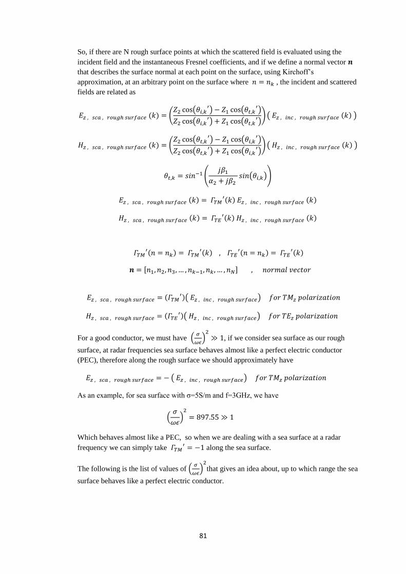
81
So, if there are N rough surface points at which the scattered field is evaluated using the
incident field and the instantaneous Fresnel coefficients, and if we define a normal vector
that describes the surface normal at each point on the surface, using Kirchoff’s
approximation, at an arbitrary point on the surface where , the incident and scattered
fields are related as
( ) ( (
) ( )
( ) (
)) ( ( ) )
( ) ( (
) ( )
( ) (
)) ( ( ) )
(
( ))
( ) ( ) ( )
( ) ( ) ( )
( )
( ) ( )
( )
[ ]
( )( )
( )( )
For a good conductor, we must have (
) , if we consider sea surface as our rough
surface, at radar frequencies sea surface behaves almost like a perfect electric conductor
(PEC), therefore along the rough surface we should approximately have
( )
As an example, for sea surface with =5S/m and f=3GHz, we have
(
)
Which behaves almost like a PEC, so when we are dealing with a sea surface at a radar
frequency we can simply take along the sea surface.
The following is the list of values of (
) that gives an idea about, up to which range the sea
surface behaves like a perfect electric conductor.
82
(
)
{
Kirchoff’s approximation is one of the most employed numerical methods. It is valid for
locally smooth surfaces and is also known as tangent plane approximation. In high
frequencies it is the same as the physical optics (PO) approximation. In this model the field
on the surface is assimilated to the field that would be produced by a tangent plane at the
same point. Thus it depends only on the Fresnel reflection coefficient at the local incidence
angle. Kirchoff’s approximation is a local approximation in the sense that the supposed field
at a surface point does not depend on other surface points[7].
Kirchoff’s approximation is especially very accurate for imposing boundary conditions
numerically with a computer program. Though the approximation is accurate in general,
small errors may occur depending on the incidence angle of the incoming wave for very
rough surfaces. The amount of error further reduces if the rough surface medium is a good
conductor, because as the conductivity of the medium increases the angle of incidence
becomes mathematically less critical. Recall that for a PEC rough surface, the local
reflection coefficients are all the same along the rough surface no matter what the incidence
angle is. As a result, for sea surfaces at radar frequencies, the accuracy of the Kirchoff’s
approximation further improves. The accuracy of the approximation also improves if the
conductivity is very small and the rough surface medium can be considered as a perfect
dielectric, similarly because the angle of incidence becomes mathematically less critical.
In summary, if
(
)
(
)
The accuracy of the Kirchoff’s approximation further increases.
6.2.2 Imposing boundary conditions on the rough surface using FEM
We know that the tangential component of the electric field is continuous at the boundary
between two different media, as stated by the boundary condition
( )
Where
( )
( )
( )
83
In medium1, the wave equation for the total field is given as
√ ( )
Which can be written as
( ) ( )
Also, the wave equations for the incident field and the scattered field are given as
Assuming that we have a 2D rough surface problem defined on the x-y plane, for a
incident wave, we have
( ) ( )
If medium 2 is an imperfectly conducting lossy media, along the boundary between the two
media, the wave equation must be modified to include the loss factor as stated
( ) ( )( )
Since the tangential component of the electric field is continuous at the interface, we have
Therefore, the following formulations are equal
( )
( ) ( )( )
As a result, at the interface the following identity is satisfied
( )
Along the boundary between the two media.
Since
is satisfied everywhere in space, at the boundary we have
( )
84
Which may also be expressed as
( )
( )
For FEM analysis, we will use the following set of formulations to determine the scattered
field everywhere in medium1
( ) ( )
( )
Recall that in 5.3, for the “element to element” varying case, the functional inside an element
was defined as
( )
∑∑ [ ∫∫( )
∫∫( ) ]
∑∑ ∫∫(
)
( )
∑∑
( ) ∑∑
( )
( )
( )
[ ]
[ ( )] [ ] [ ] [ ( )]
( ) ∫∫
( ) ∫∫
( )
( )
( ) ( )
( ) [ ∫∫( )
∫∫( ) ]
( ) [
( )
( ) ( )
( )
( ) ( )
( )
( ) ( )
] ( ) [
( )
( ) ( )
( )
( ) ( )
( )
( ) ( )
]
( )
[ ]
[ ( )] [ ] [ ] [ ( )]
Summing for all elements, we have
85
( ) ∑ ( )
( )
[ ] [ ] [ ] [ ] [ ]
Therefore, the FEM solution is given by (5)
( )
( )
∑[
]
∑
( )
For elements, which have one of its three sides at the boundary, we should introduce the
source and loss factor, since
( ) ( )
( )
{
{
should be evaluated at the center of each surface element.
Therefore, for surface elements having one complete side (two nodes) at the boundary
( )
∑∑ [ ∫∫( )
∫∫( ) ]
∑∑ ∫∫(
)
For all of the other elements
( )
∑∑ [ ∫∫( )
∫∫( ) ]
The rest of the procedure is to assemble all elements as described previously, after forming
the global coefficient matrix and the source vector, we can solve (5) to get the field values
everywhere in medium1. After solving the linear system (5) , we can see that the field values
at the boundary automatically satisfy the impedance boundary condition along the whole
boundary. The resulting linear system can be written in its expanded form as
86
•
•
Section 5.3 can be revisited to recall the assembling procedure of the elements.
6.3 Examples of rough surface scattering using FEM
Until now we have described the fundamental concepts that are necessary for solving the
problem of rough surface scattering using FEM, basically we have discussed the followings
1)Mesh generation for nonrectangular regions.
2)Basics of the finite element method and its formulation.
3)Locally conformal perfectly matched layer.
4)Imposing boundary condition on a given rough surface.
Once these concepts are fully understood and implemented, FEM can be applied on
scattering and radiation problems.
We will now see some examples of rough surface scattering using FEM, here we will
concentrate on four parameters to specify a rough surface scattering problem
1)PML width along x and y directions.
2)Frequency of the incident wave
3)Conductivity of the rough surface boundary.
4)Mesh size of the computational region(excluding PML).
Angle measure: Angle is measured from the positive x axis, that is,
Ф= for positive x axis, Ф= for positive y axis and Ф= for negative x axis.
Incident wave: The incident wave is a uniform plane wave and has an amplitude of 100V/m,
its incidence angle will be specified in each example.
( )
λ : Wavelength , : Standard deviation value of the surface roughness
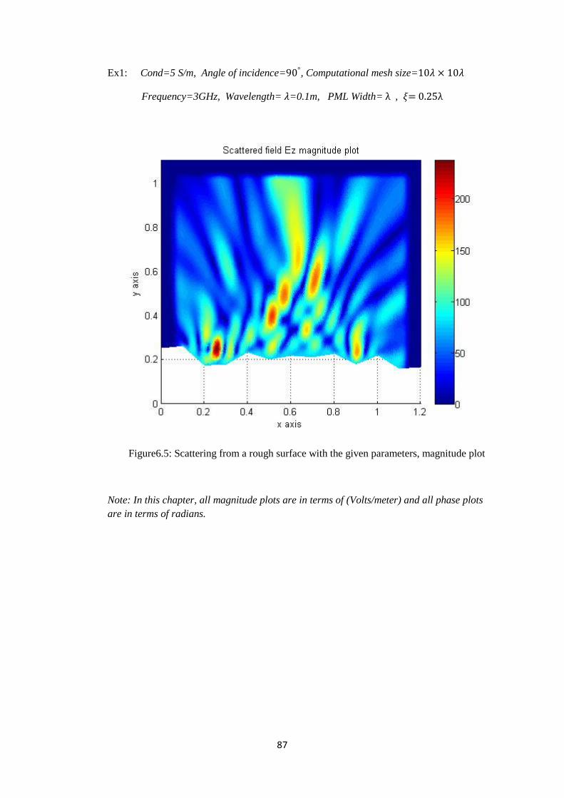
87
Ex1: Cond=5 S/m, Angle of incidence= , Computational mesh size=
Frequency=3GHz, Wavelength= =0.1m, PML Width= ,
Figure6.5: Scattering from a rough surface with the given parameters, magnitude plot
Note: In this chapter, all magnitude plots are in terms of (Volts/meter) and all phase plots
are in terms of radians.
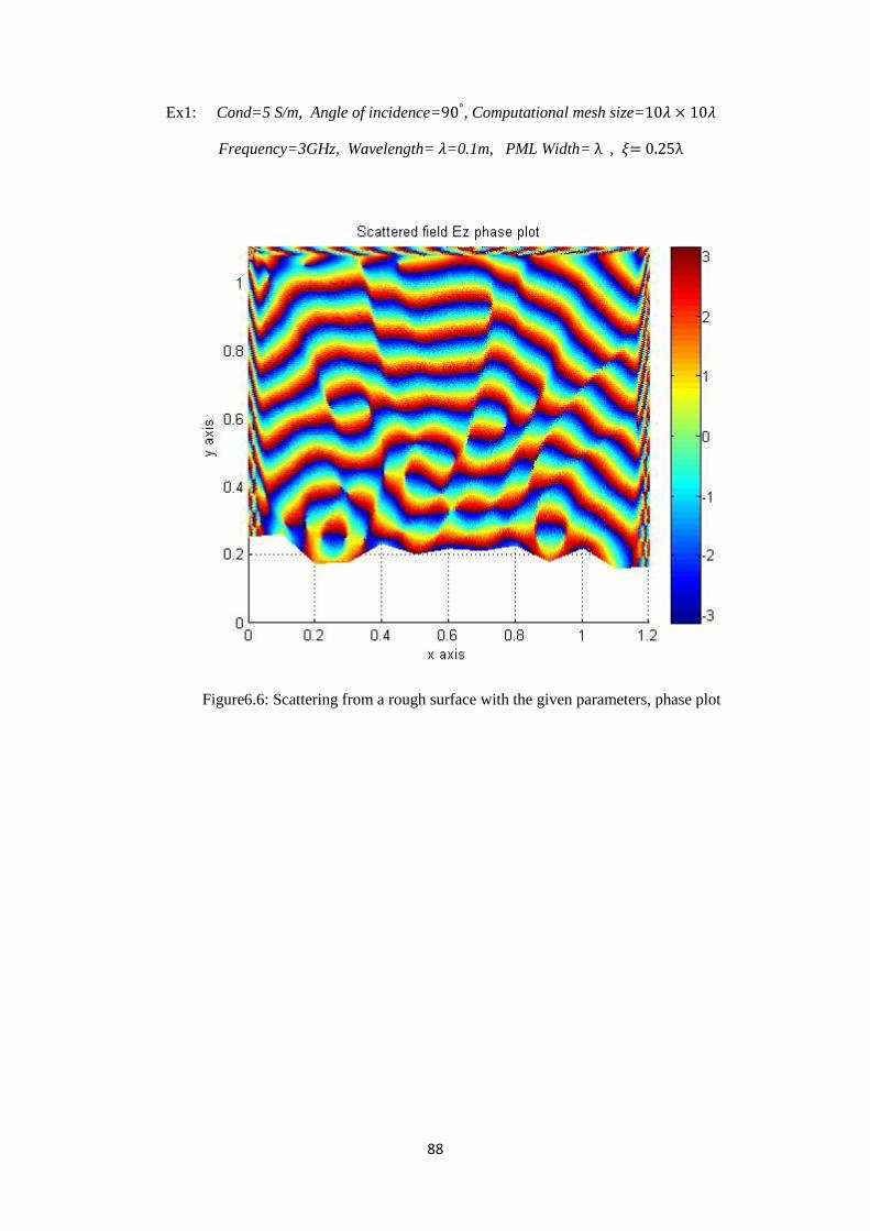
88
Ex1: Cond=5 S/m, Angle of incidence= , Computational mesh size=
Frequency=3GHz, Wavelength= =0.1m, PML Width= ,
Figure6.6: Scattering from a rough surface with the given parameters, phase plot
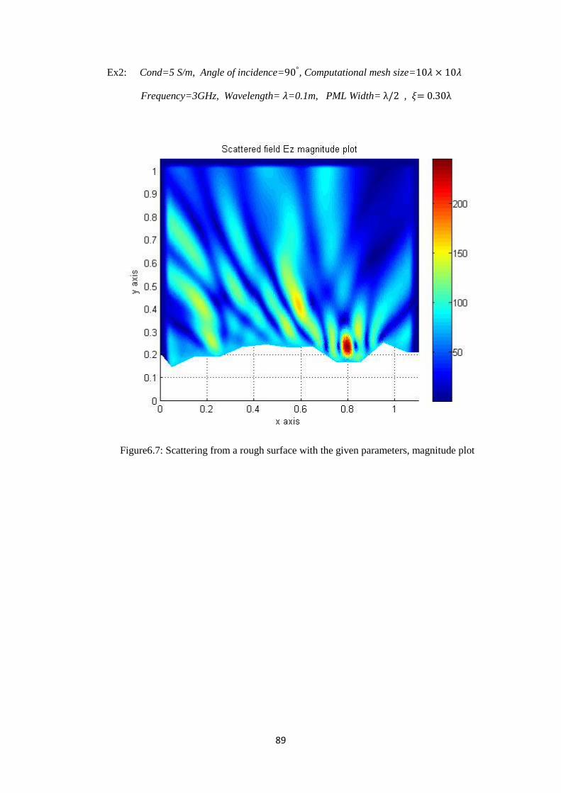
89
Ex2: Cond=5 S/m, Angle of incidence= , Computational mesh size=
Frequency=3GHz, Wavelength= =0.1m, PML Width= ,
Figure6.7: Scattering from a rough surface with the given parameters, magnitude plot
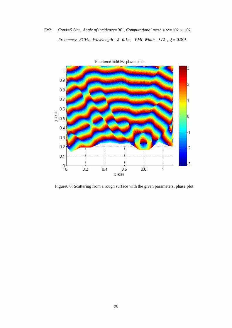
90
Ex2: Cond=5 S/m, Angle of incidence= , Computational mesh size=
Frequency=3GHz, Wavelength= =0.1m, PML Width= ,
Figure6.8: Scattering from a rough surface with the given parameters, phase plot
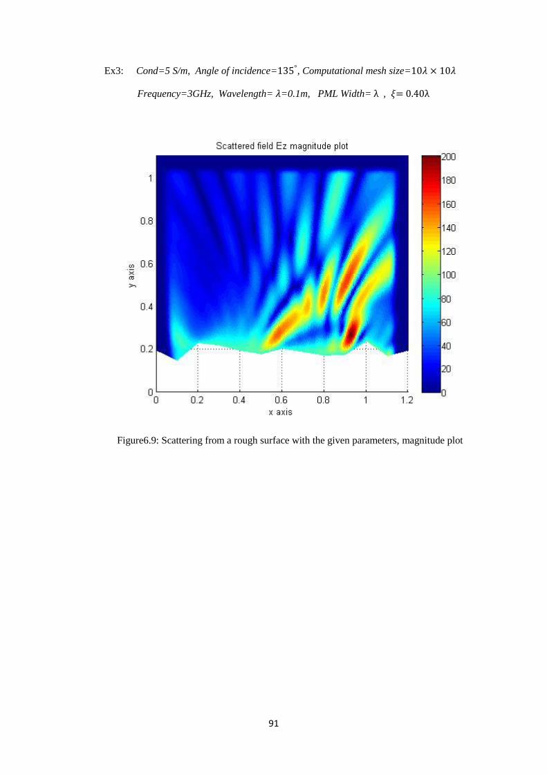
91
Ex3: Cond=5 S/m, Angle of incidence= , Computational mesh size=
Frequency=3GHz, Wavelength= =0.1m, PML Width= ,
Figure6.9: Scattering from a rough surface with the given parameters, magnitude plot

92
Ex3: Cond=5 S/m, Angle of incidence= , Computational mesh size=
Frequency=3GHz, Wavelength= =0.1m, PML Width= ,
Figure6.10: Scattering from a rough surface with the given parameters, phase plot
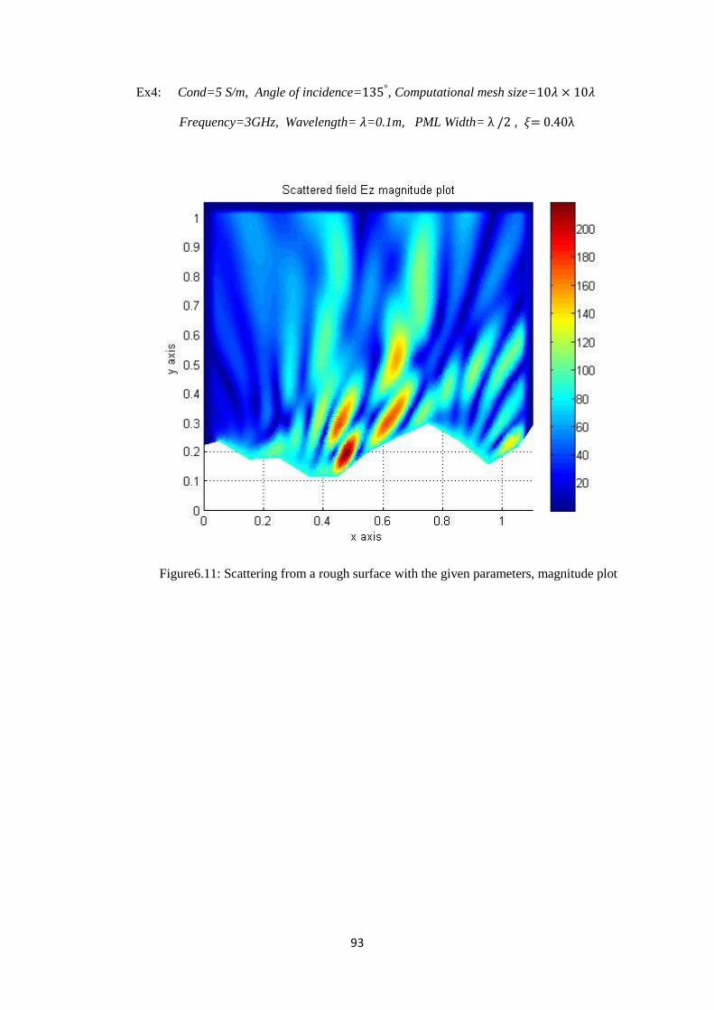
93
Ex4: Cond=5 S/m, Angle of incidence= , Computational mesh size=
Frequency=3GHz, Wavelength= =0.1m, PML Width= ,
Figure6.11: Scattering from a rough surface with the given parameters, magnitude plot
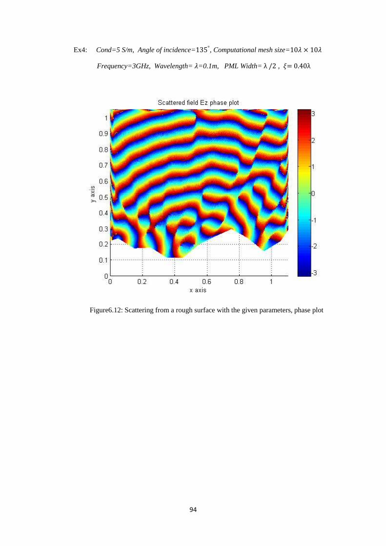
94
Ex4: Cond=5 S/m, Angle of incidence= , Computational mesh size=
Frequency=3GHz, Wavelength= =0.1m, PML Width= ,
Figure6.12: Scattering from a rough surface with the given parameters, phase plot
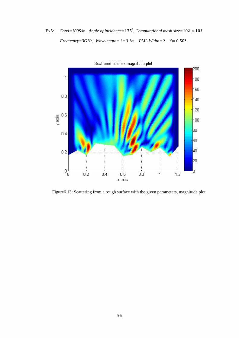
95
Ex5: Cond=100S/m, Angle of incidence= , Computational mesh size=
Frequency=3GHz, Wavelength= =0.1m, PML Width= ,
Figure6.13: Scattering from a rough surface with the given parameters, magnitude plot
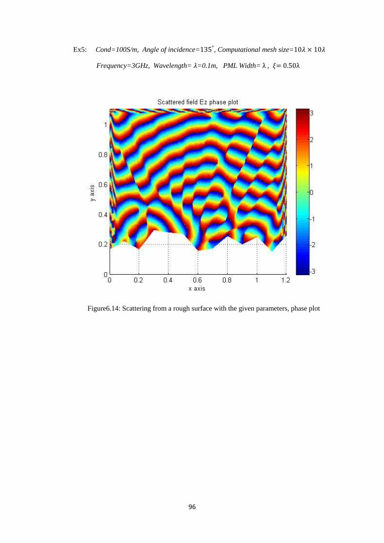
96
Ex5: Cond=100S/m, Angle of incidence= , Computational mesh size=
Frequency=3GHz, Wavelength= =0.1m, PML Width= ,
Figure6.14: Scattering from a rough surface with the given parameters, phase plot
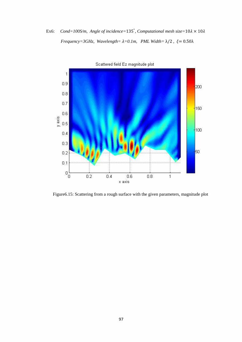
97
Ex6: Cond=100S/m, Angle of incidence= , Computational mesh size=
Frequency=3GHz, Wavelength= =0.1m, PML Width= , =
Figure6.15: Scattering from a rough surface with the given parameters, magnitude plot
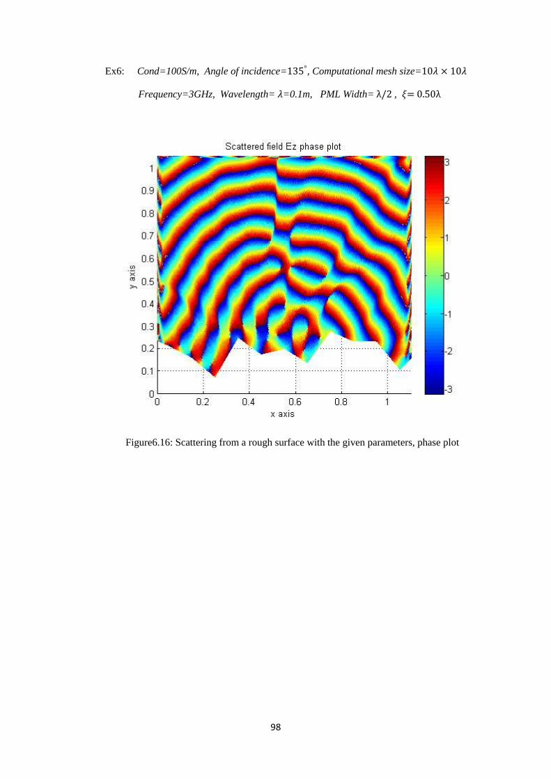
98
Ex6: Cond=100S/m, Angle of incidence= , Computational mesh size=
Frequency=3GHz, Wavelength= =0.1m, PML Width= ,
Figure6.16: Scattering from a rough surface with the given parameters, phase plot
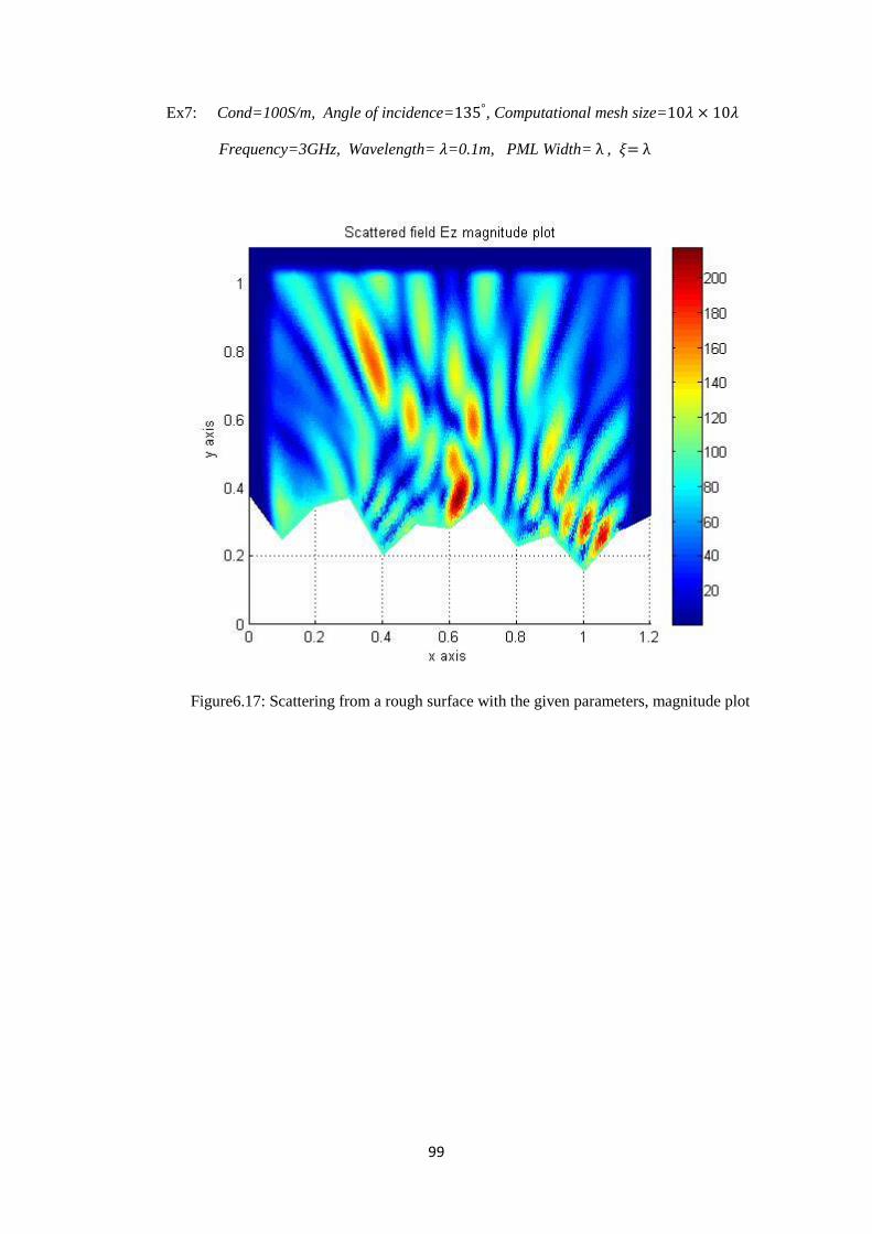
99
Ex7: Cond=100S/m, Angle of incidence= , Computational mesh size=
Frequency=3GHz, Wavelength= =0.1m, PML Width= ,
Figure6.17: Scattering from a rough surface with the given parameters, magnitude plot
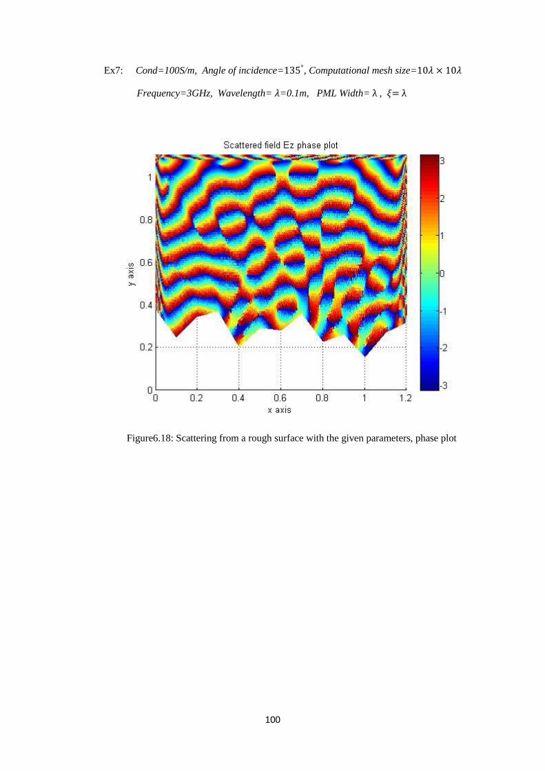
100
Ex7: Cond=100S/m, Angle of incidence= , Computational mesh size=
Frequency=3GHz, Wavelength= =0.1m, PML Width= ,
Figure6.18: Scattering from a rough surface with the given parameters, phase plot
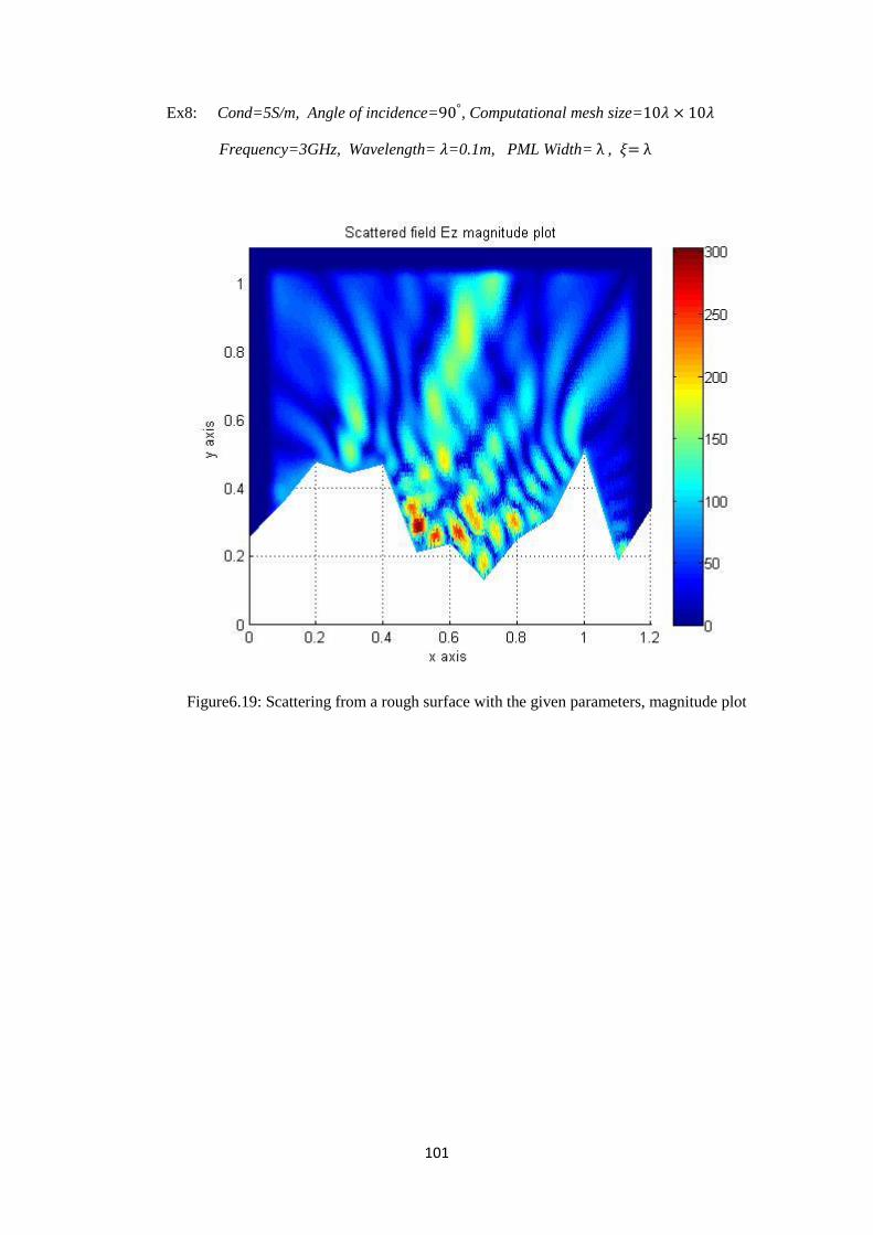
101
Ex8: Cond=5S/m, Angle of incidence= , Computational mesh size=
Frequency=3GHz, Wavelength= =0.1m, PML Width= ,
Figure6.19: Scattering from a rough surface with the given parameters, magnitude plot
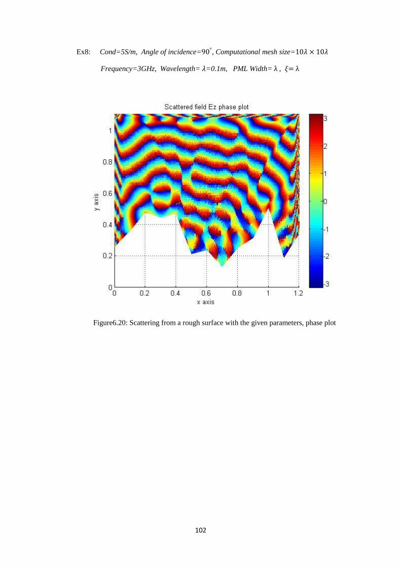
102
Ex8: Cond=5S/m, Angle of incidence= , Computational mesh size=
Frequency=3GHz, Wavelength= =0.1m, PML Width= ,
Figure6.20: Scattering from a rough surface with the given parameters, phase plot
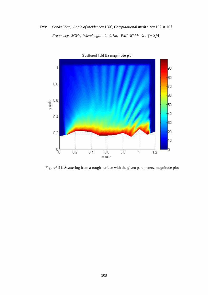
103
Ex9: Cond=5S/m, Angle of incidence= , Computational mesh size=
Frequency=3GHz, Wavelength= =0.1m, PML Width= ,
Figure6.21: Scattering from a rough surface with the given parameters, magnitude plot
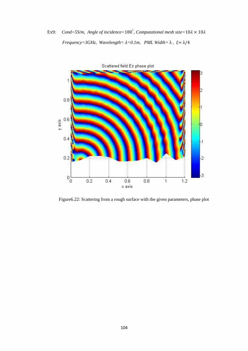
104
Ex9: Cond=5S/m, Angle of incidence= , Computational mesh size=
Frequency=3GHz, Wavelength= =0.1m, PML Width= ,
Figure6.22: Scattering from a rough surface with the given parameters, phase plot
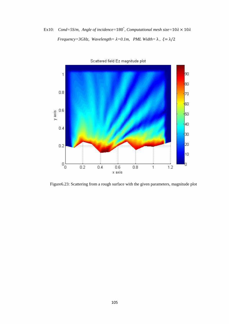
105
Ex10: Cond=5S/m, Angle of incidence= , Computational mesh size=
Frequency=3GHz, Wavelength= =0.1m, PML Width= ,
Figure6.23: Scattering from a rough surface with the given parameters, magnitude plot
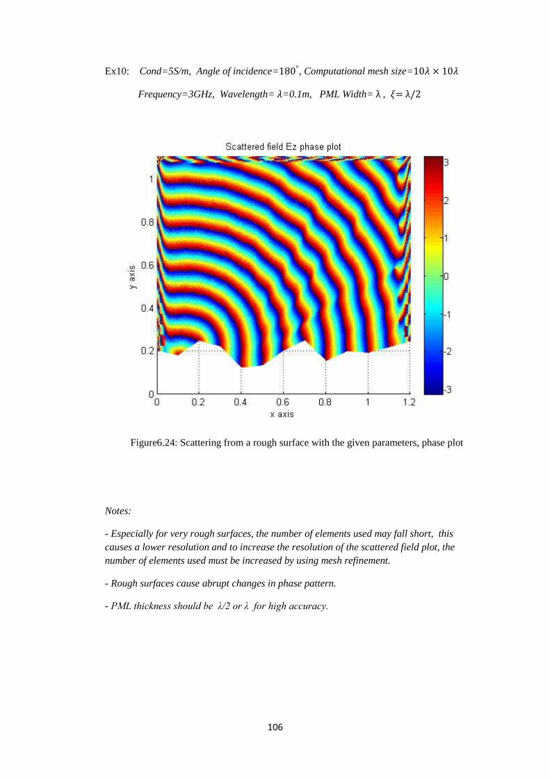
106
Ex10: Cond=5S/m, Angle of incidence= , Computational mesh size=
Frequency=3GHz, Wavelength= =0.1m, PML Width= ,
Figure6.24: Scattering from a rough surface with the given parameters, phase plot
Notes:
- Especially for very rough surfaces, the number of elements used may fall short, this
causes a lower resolution and to increase the resolution of the scattered field plot, the
number of elements used must be increased by using mesh refinement.
- Rough surfaces cause abrupt changes in phase pattern.
- PML thickness should be λ/2 or λ for high accuracy.
107
6.4 Comparison of FEM solutions with analytical solutions
FEM is based on the functionals of partial differential equations whose solutions are desired,
we have previously derived the functional for the Helmholtz equation as
√
( )
∬[ (
) (
) ]
( )
∬[ ]
The FEM solution of the Helmholtz equation is obtained by minimizing its functional at
every point in the solution region as
( )
∑ [
]
If there are no sources in the solution region the solution becomes
( )
∑ [
]
Recall that in chapter2, the most general form of wave equation was given as
Since our domain of interest in analyzing the rough surface problem is lossless and
contains no impressed sources, we have ( =0, =0, =0 , =0) , therefore the general form of the wave equation simplifies into the homogenous Helmholtz equation
However, when an incident plane wave hits the rough surface, it induces an electrical current
distribution on the rough surface, therefore our rough surface scattering problem is not
sourceless along the rough surface boundary. The incident plane wave can be thought as a
conduction current source along the rough surface boundary and the wave equation can be
modified as
= Impressed electric current density (amperes/square meter)
= Conduction electric current density (amperes/square meter)
If the incident wave is a plane wave, this equation becomes a scalar equation and can
be written as
Where J= is the source current density along the rough surface.
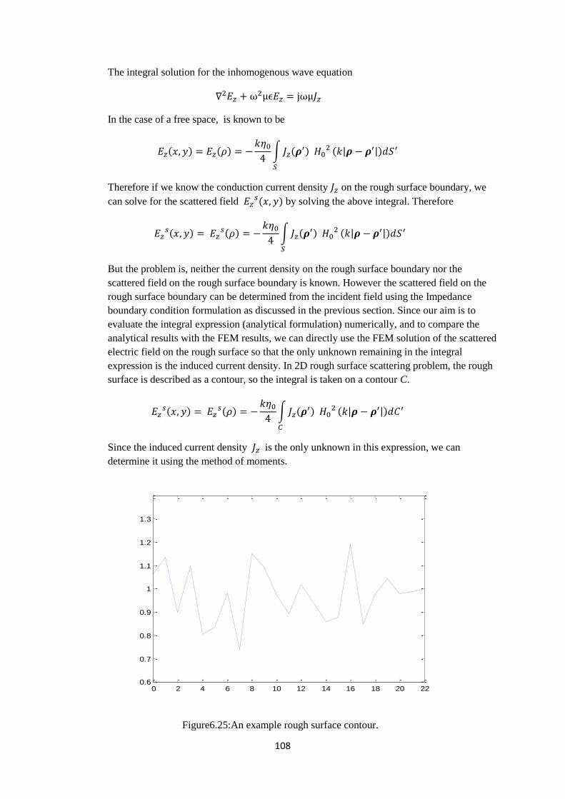
108
The integral solution for the inhomogenous wave equation
In the case of a free space, is known to be
( ) ( )
∫ (
)
( )
Therefore if we know the conduction current density on the rough surface boundary, we
can solve for the scattered field ( ) by solving the above integral. Therefore
( )
( )
∫ (
)
( )
But the problem is, neither the current density on the rough surface boundary nor the
scattered field on the rough surface boundary is known. However the scattered field on the
rough surface boundary can be determined from the incident field using the Impedance
boundary condition formulation as discussed in the previous section. Since our aim is to
evaluate the integral expression (analytical formulation) numerically, and to compare the
analytical results with the FEM results, we can directly use the FEM solution of the scattered
electric field on the rough surface so that the only unknown remaining in the integral
expression is the induced current density. In 2D rough surface scattering problem, the rough
surface is described as a contour, so the integral is taken on a contour C.
( )
( )
∫ (
)
( )
Since the induced current density is the only unknown in this expression, we can
determine it using the method of moments.
Figure6.25:An example rough surface contour.
0 2 4 6 8 10 12 14 16 18 20 220.6
0.7
0.8
0.9
1
1.1
1.2
1.3
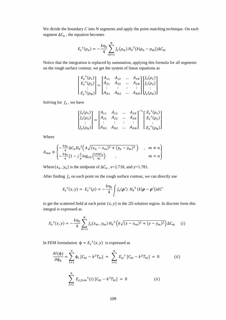
109
We divide the boundary C into N segments and apply the point matching technique. On each
segment , the equation becomes
( )
∑ ( )
( )
Notice that the integration is replaced by summation, applying this formula for all segments
on the rough surface contour, we get the system of linear equations as
[
( )
( )
( )]
[
] [
( )
( )
( )
]
Solving for , we have
[
( )
( )
( )
] [
]
[
( )
( )
( )]
Where
{
( √( ) ( ) )
[
(
)
}
Where{ is the midpoint of , e=2.718, and 𝛾=1.781.
After finding on each point on the rough surface contour, we can directly use
( )
( )
∫ (
)
( )
to get the scattered field at each point { in the 2D solution region. In discrete form this
integral is expressed as
( )
∑ ( )
( √( ) ( ) ) ( )
In FEM formulation ( ) is expressed as
( )
∑ [
] ∑ [
] ( )
∑ ( ) [
] ( )
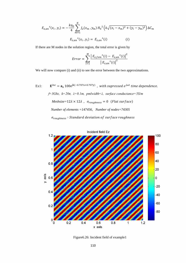
110
( )
∑ ( )
( √( ) ( ) )
( )
( ) ( )
If there are M nodes in the solution region, the total error is given by
∑|
( ) ( )|
| ( )|
We will now compare (i) and (ii) to see the error between the two approximations.
Ex1: ( )
f=3Ghz, k=20π, λ=0.1m, pmlwidth=λ, surface conductance=5S/m
Meshsize= , ( )
Number of elements =147456, Number of nodes=74305
Figure6.26: Incident field of example1
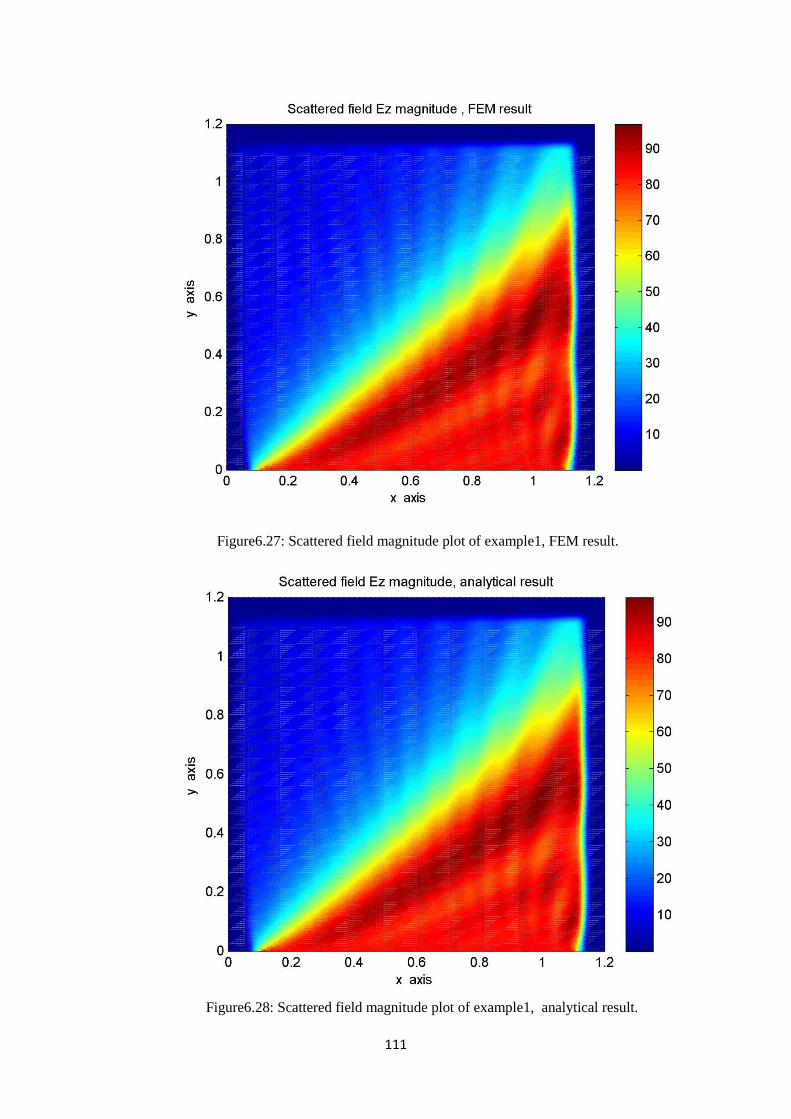
111
Figure6.27: Scattered field magnitude plot of example1, FEM result.
Figure6.28: Scattered field magnitude plot of example1, analytical result.
112
Figure6.29: Scattered field phase plot of example1, FEM result.
Figure6.30: Scattered field phase plot of example1, analytical result.
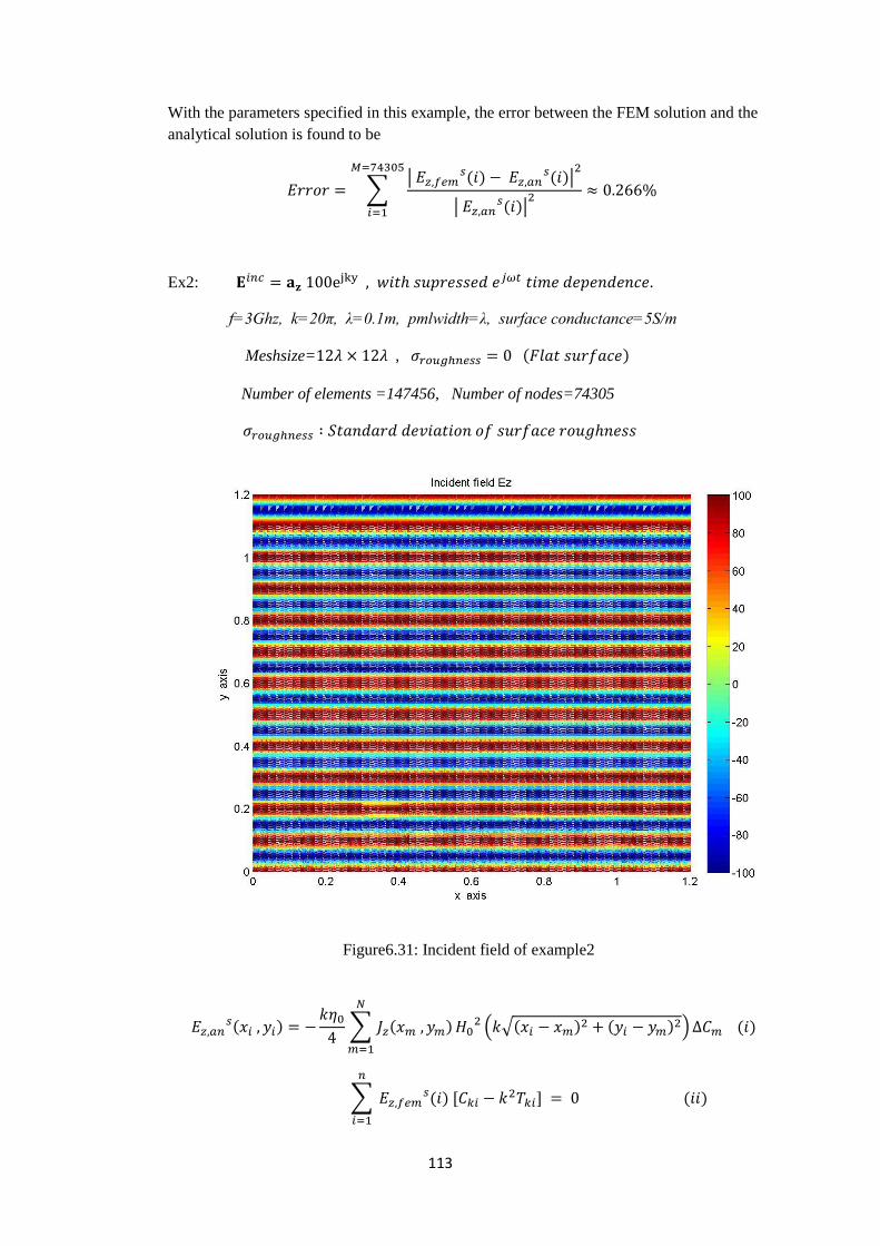
113
With the parameters specified in this example, the error between the FEM solution and the
analytical solution is found to be
∑|
( ) ( )|
| ( )|
Ex2:
f=3Ghz, k=20π, λ=0.1m, pmlwidth=λ, surface conductance=5S/m
Meshsize= , ( )
Number of elements =147456, Number of nodes=74305
Figure6.31: Incident field of example2
( )
∑ ( )
( √( ) ( ) ) ( )
∑ ( ) [
] ( )
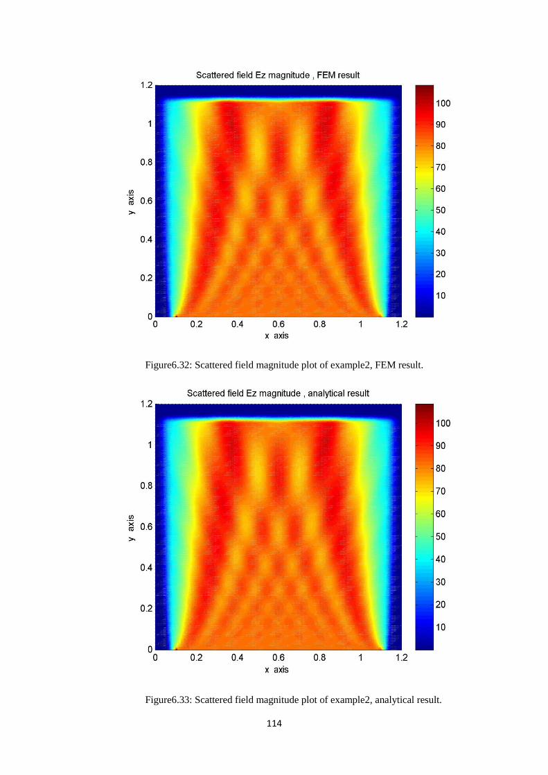
114
Figure6.32: Scattered field magnitude plot of example2, FEM result.
Figure6.33: Scattered field magnitude plot of example2, analytical result.
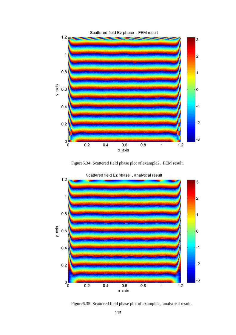
115
Figure6.34: Scattered field phase plot of example2, FEM result.
Figure6.35: Scattered field phase plot of example2, analytical result.
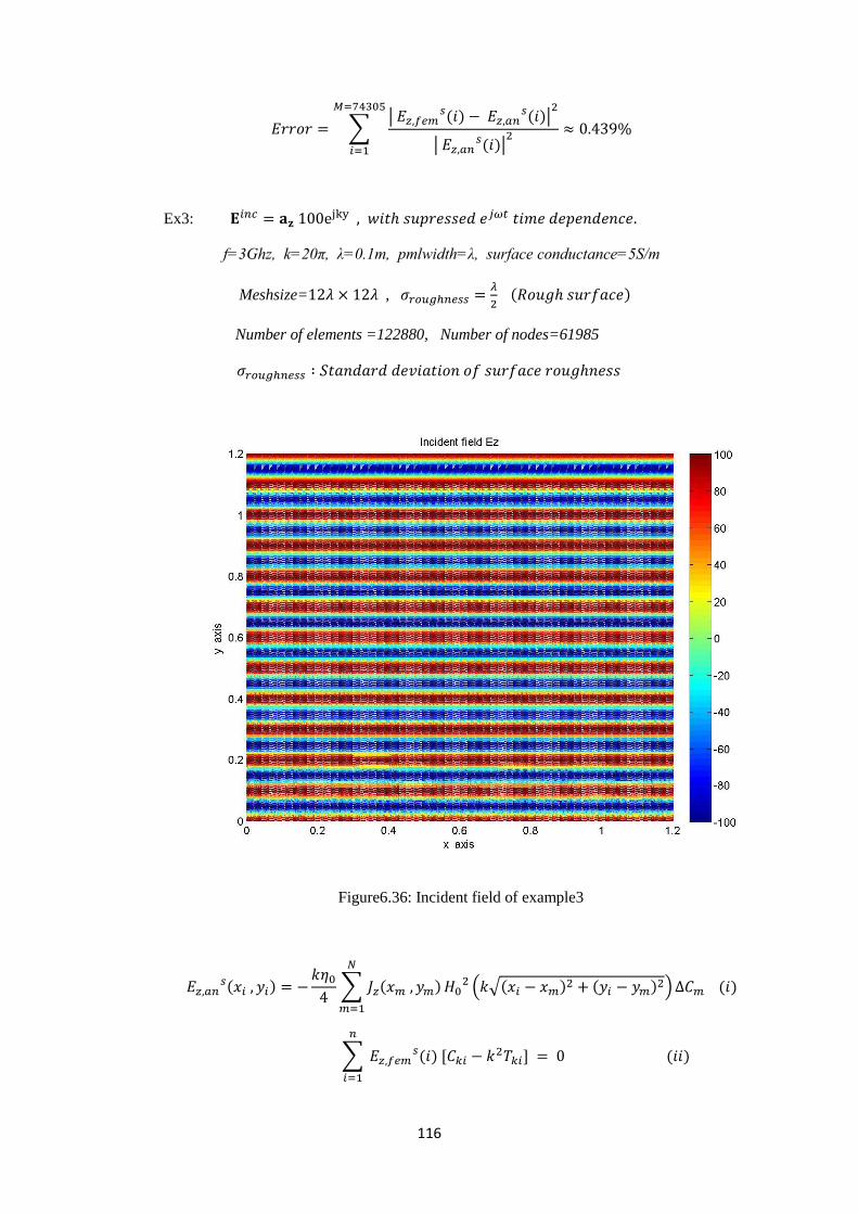
116
∑|
( ) ( )|
| ( )|
Ex3:
f=3Ghz, k=20π, λ=0.1m, pmlwidth=λ, surface conductance=5S/m
Meshsize= ,
( )
Number of elements =122880, Number of nodes=61985
Figure6.36: Incident field of example3
( )
∑ ( )
( √( ) ( ) ) ( )
∑ ( ) [
] ( )
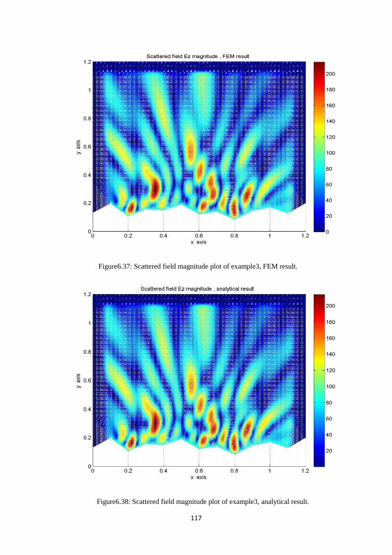
117
Figure6.37: Scattered field magnitude plot of example3, FEM result.
Figure6.38: Scattered field magnitude plot of example3, analytical result.
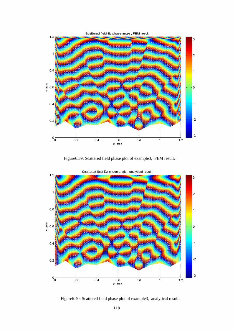
118
Figure6.39: Scattered field phase plot of example3, FEM result.
Figure6.40: Scattered field phase plot of example3, analytical result.
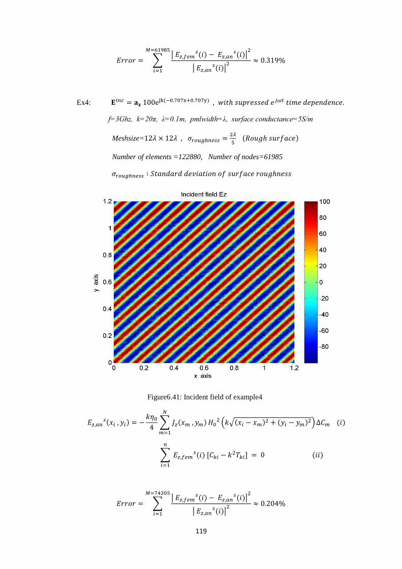
119
∑|
( ) ( )|
| ( )|
Ex4: ( )
f=3Ghz, k=20π, λ=0.1m, pmlwidth=λ, surface conductance=5S/m
Meshsize= ,
( )
Number of elements =122880, Number of nodes=61985
Figure6.41: Incident field of example4
( )
∑ ( )
( √( ) ( ) ) ( )
∑ ( ) [
] ( )
∑|
( ) ( )|
| ( )|
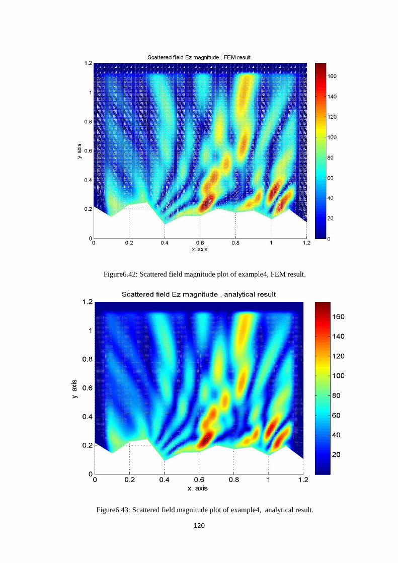
120
Figure6.42: Scattered field magnitude plot of example4, FEM result.
Figure6.43: Scattered field magnitude plot of example4, analytical result.
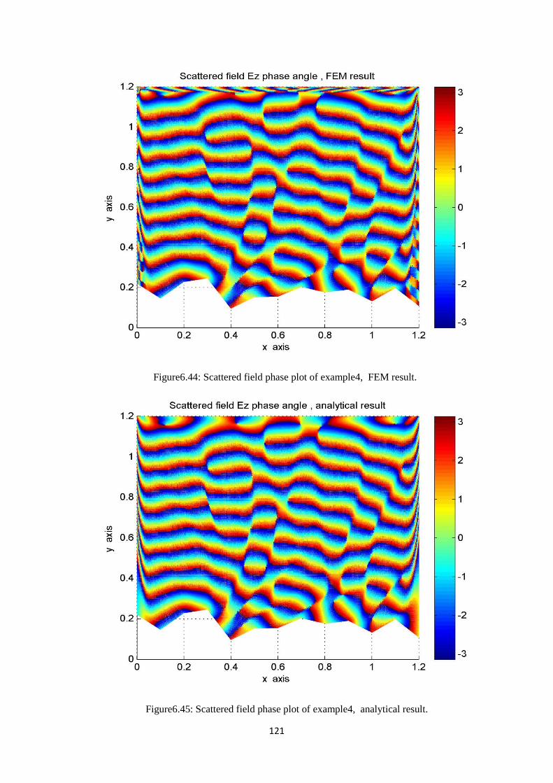
121
Figure6.44: Scattered field phase plot of example4, FEM result.
Figure6.45: Scattered field phase plot of example4, analytical result.
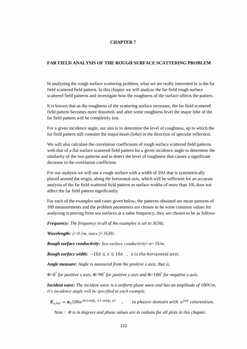
122
CHAPTER 7
FAR FIELD ANALYSIS OF THE ROUGH SURFACE SCATTERING PROBLEM
In analyzing the rough surface scattering problem, what we are really interested in is the far
field scattered field pattern. In this chapter we will analyze the far field rough surface
scattered field patterns and investigate how the roughness of the surface affects the pattern.
It is known that as the roughness of the scattering surface increases, the far field scattered
field pattern becomes more distorted, and after some roughness level the major lobe of the
far field pattern will be completely lost.
For a given incidence angle, our aim is to determine the level of roughness, up to which the
far field pattern still contains the major beam (lobe) in the direction of specular reflection.
We will also calculate the correlation coefficients of rough surface scattered field patterns
with that of a flat surface scattered field pattern for a given incidence angle to determine the
similarity of the two patterns and to detect the level of roughness that causes a significant
decrease in the correlation coefficient.
For our analysis we will use a rough surface with a width of that is symmetrically
placed around the origin, along the horizontal axis, which will be sufficient for an accurate
analysis of the far field scattered field pattern as surface widths of more than 10λ does not
affect the far field pattern significantly.
For each of the examples and cases given below, the patterns obtained are mean patterns of
100 measurements and the problem parameters are chosen to be some common values for
analyzing scattering from sea surfaces at a radar frequency, they are chosen to be as follows
Frequency: The frequency in all of the examples is set to 3GHz.
Wavelength: λ=0.1m, since f=3GHz.
Rough surface conductivity: Sea surface conductivity=σ=5S/m.
Rough surface width:
Angle measure: Angle is measured from the positive x axis, that is,
Ф= for positive x axis, Ф= for positive y axis and Ф= for negative x axis.
Incident wave: The incident wave is a uniform plane wave and has an amplitude of 100V/m,
it’s incidence angle will be specified in each example.
( )
Note : Φ is in degrees and phase values are in radians for all plots in this chapter.
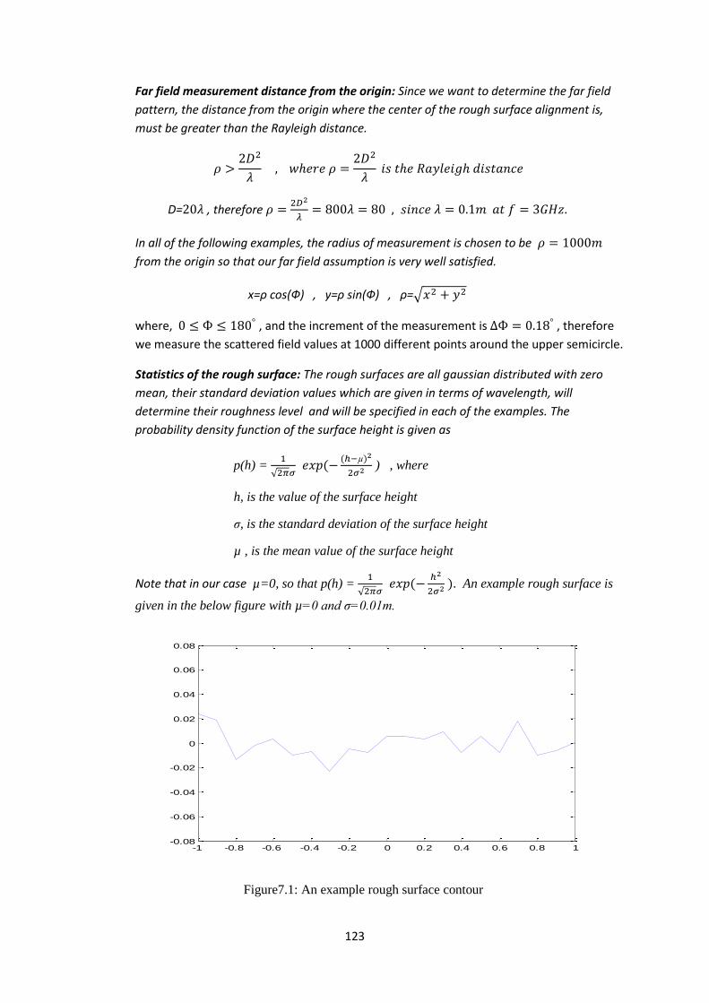
123
Far field measurement distance from the origin: Since we want to determine the far field
pattern, the distance from the origin where the center of the rough surface alignment is,
must be greater than the Rayleigh distance.
D= , therefore
In all of the following examples, the radius of measurement is chosen to be
from the origin so that our far field assumption is very well satisfied.
x=ρ cos(Ф) , y=ρ sin(Ф) , ρ=√
where, , and the increment of the measurement is , therefore
we measure the scattered field values at 1000 different points around the upper semicircle.
Statistics of the rough surface: The rough surfaces are all gaussian distributed with zero
mean, their standard deviation values which are given in terms of wavelength, will
determine their roughness level and will be specified in each of the examples. The
probability density function of the surface height is given as
p(h) =
√ (
( )
) , where
h, is the value of the surface height
σ, is the standard deviation of the surface height
µ , is the mean value of the surface height
Note that in our case µ=0, so that p(h) =
√ (
). An example rough surface is
given in the below figure with µ=0 and σ=0.01m.
Figure7.1: An example rough surface contour
-1 -0.8 -0.6 -0.4 -0.2 0 0.2 0.4 0.6 0.8 1-0.08
-0.06
-0.04
-0.02
0
0.02
0.04
0.06
0.08
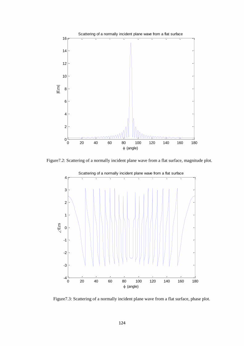
124
Figure7.2: Scattering of a normally incident plane wave from a flat surface, magnitude plot.
Figure7.3: Scattering of a normally incident plane wave from a flat surface, phase plot.
0 20 40 60 80 100 120 140 160 1800
2
4
6
8
10
12
14
16
(angle)
|Ezs|
Scattering of a normally incident plane wave from a flat surface
0 20 40 60 80 100 120 140 160 180-4
-3
-2
-1
0
1
2
3
4
(angle)
E
zs
Scattering of a normally incident plane wave from a flat surface
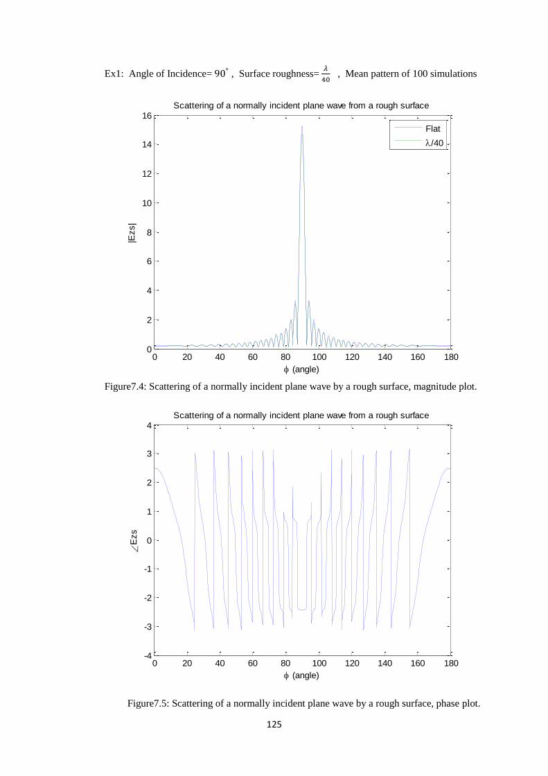
125
Ex1: Angle of Incidence= , Surface roughness=
, Mean pattern of 100 simulations
Figure7.4: Scattering of a normally incident plane wave by a rough surface, magnitude plot.
Figure7.5: Scattering of a normally incident plane wave by a rough surface, phase plot.
0 20 40 60 80 100 120 140 160 1800
2
4
6
8
10
12
14
16
(angle)
|Ezs|
Scattering of a normally incident plane wave from a rough surface
Flat
/40
0 20 40 60 80 100 120 140 160 180-4
-3
-2
-1
0
1
2
3
4
(angle)
E
zs
Scattering of a normally incident plane wave from a rough surface
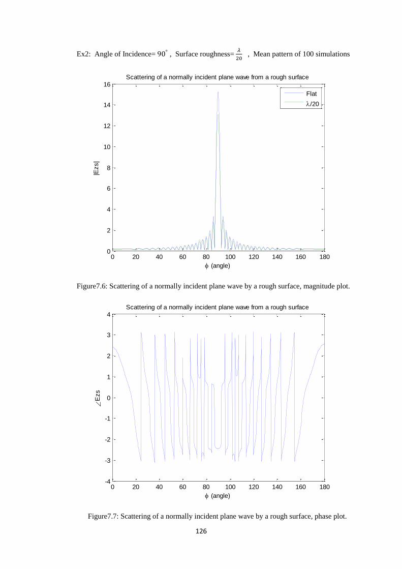
126
Ex2: Angle of Incidence= , Surface roughness=
, Mean pattern of 100 simulations
Figure7.6: Scattering of a normally incident plane wave by a rough surface, magnitude plot.
Figure7.7: Scattering of a normally incident plane wave by a rough surface, phase plot.
0 20 40 60 80 100 120 140 160 1800
2
4
6
8
10
12
14
16
(angle)
|Ezs|
Scattering of a normally incident plane wave from a rough surface
Flat
/20
0 20 40 60 80 100 120 140 160 180-4
-3
-2
-1
0
1
2
3
4
(angle)
E
zs
Scattering of a normally incident plane wave from a rough surface
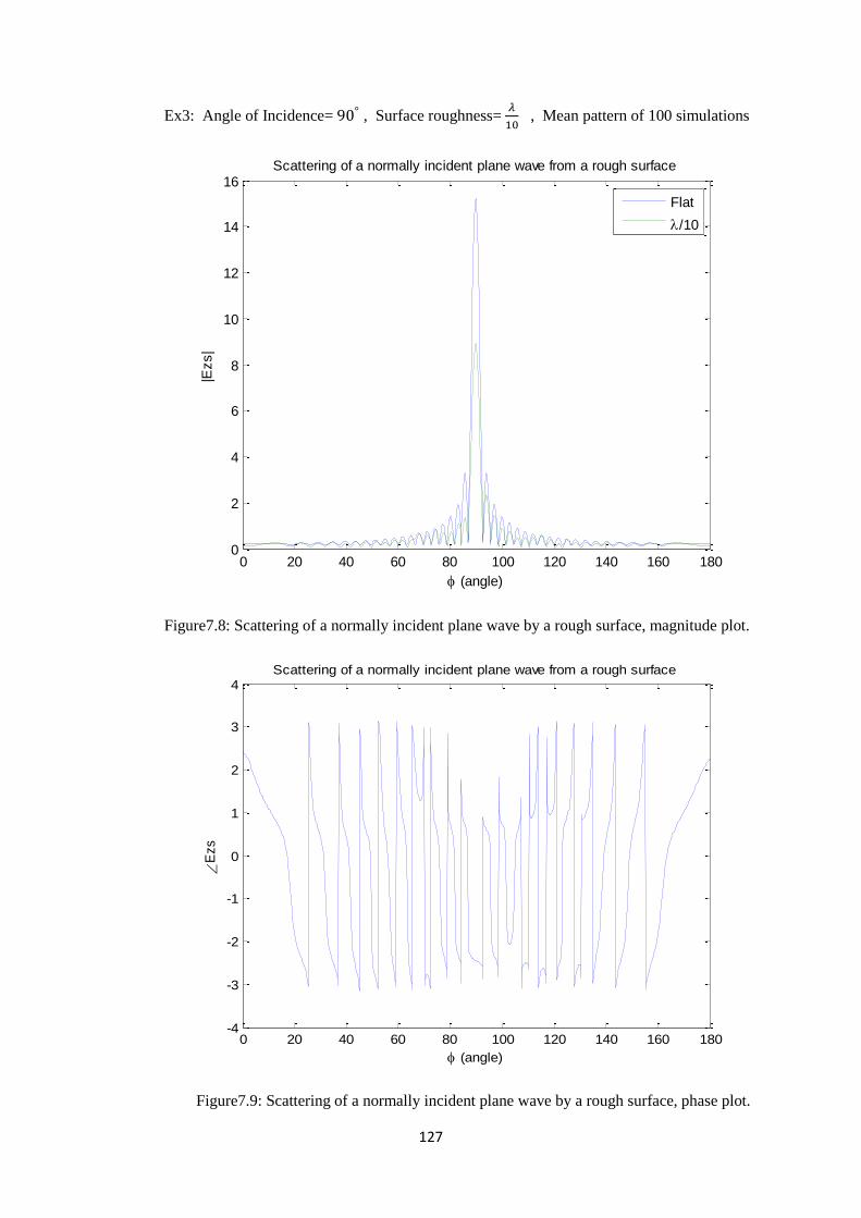
127
Ex3: Angle of Incidence= , Surface roughness=
, Mean pattern of 100 simulations
Figure7.8: Scattering of a normally incident plane wave by a rough surface, magnitude plot.
Figure7.9: Scattering of a normally incident plane wave by a rough surface, phase plot.
0 20 40 60 80 100 120 140 160 1800
2
4
6
8
10
12
14
16
(angle)
|Ezs|
Scattering of a normally incident plane wave from a rough surface
Flat
/10
0 20 40 60 80 100 120 140 160 180-4
-3
-2
-1
0
1
2
3
4
(angle)
E
zs
Scattering of a normally incident plane wave from a rough surface
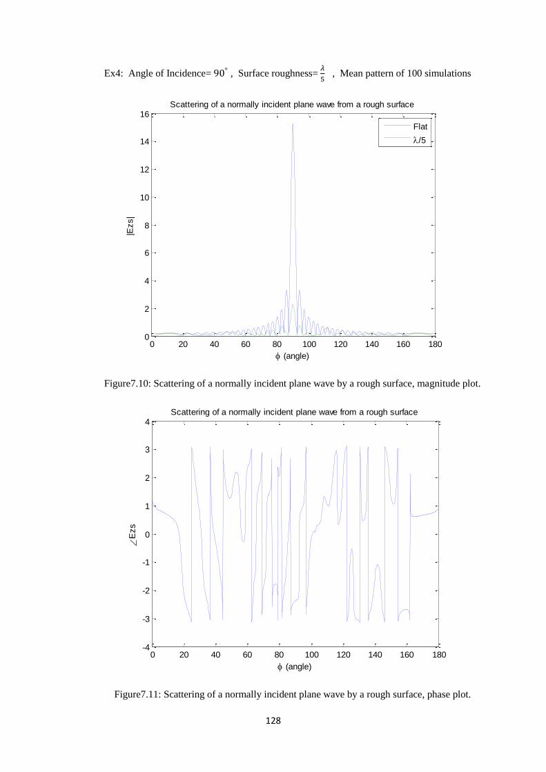
128
Ex4: Angle of Incidence= , Surface roughness=
, Mean pattern of 100 simulations
Figure7.10: Scattering of a normally incident plane wave by a rough surface, magnitude plot.
Figure7.11: Scattering of a normally incident plane wave by a rough surface, phase plot.
0 20 40 60 80 100 120 140 160 1800
2
4
6
8
10
12
14
16
(angle)
|Ezs|
Scattering of a normally incident plane wave from a rough surface
Flat
/5
0 20 40 60 80 100 120 140 160 180-4
-3
-2
-1
0
1
2
3
4
(angle)
E
zs
Scattering of a normally incident plane wave from a rough surface
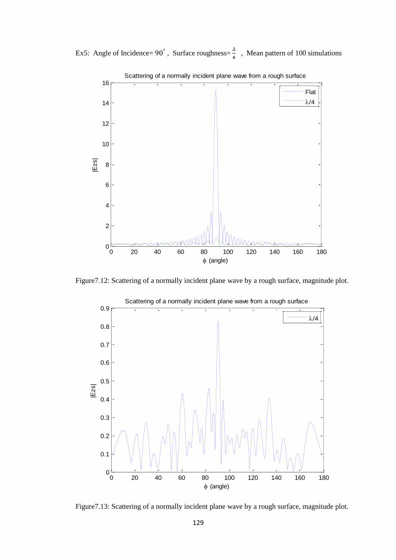
129
Ex5: Angle of Incidence= , Surface roughness=
, Mean pattern of 100 simulations
Figure7.12: Scattering of a normally incident plane wave by a rough surface, magnitude plot.
Figure7.13: Scattering of a normally incident plane wave by a rough surface, magnitude plot.
0 20 40 60 80 100 120 140 160 1800
2
4
6
8
10
12
14
16
(angle)
|Ezs|
Scattering of a normally incident plane wave from a rough surface
Flat
/4
0 20 40 60 80 100 120 140 160 1800
0.1
0.2
0.3
0.4
0.5
0.6
0.7
0.8
0.9
(angle)
|Ezs|
Scattering of a normally incident plane wave from a rough surface
/4
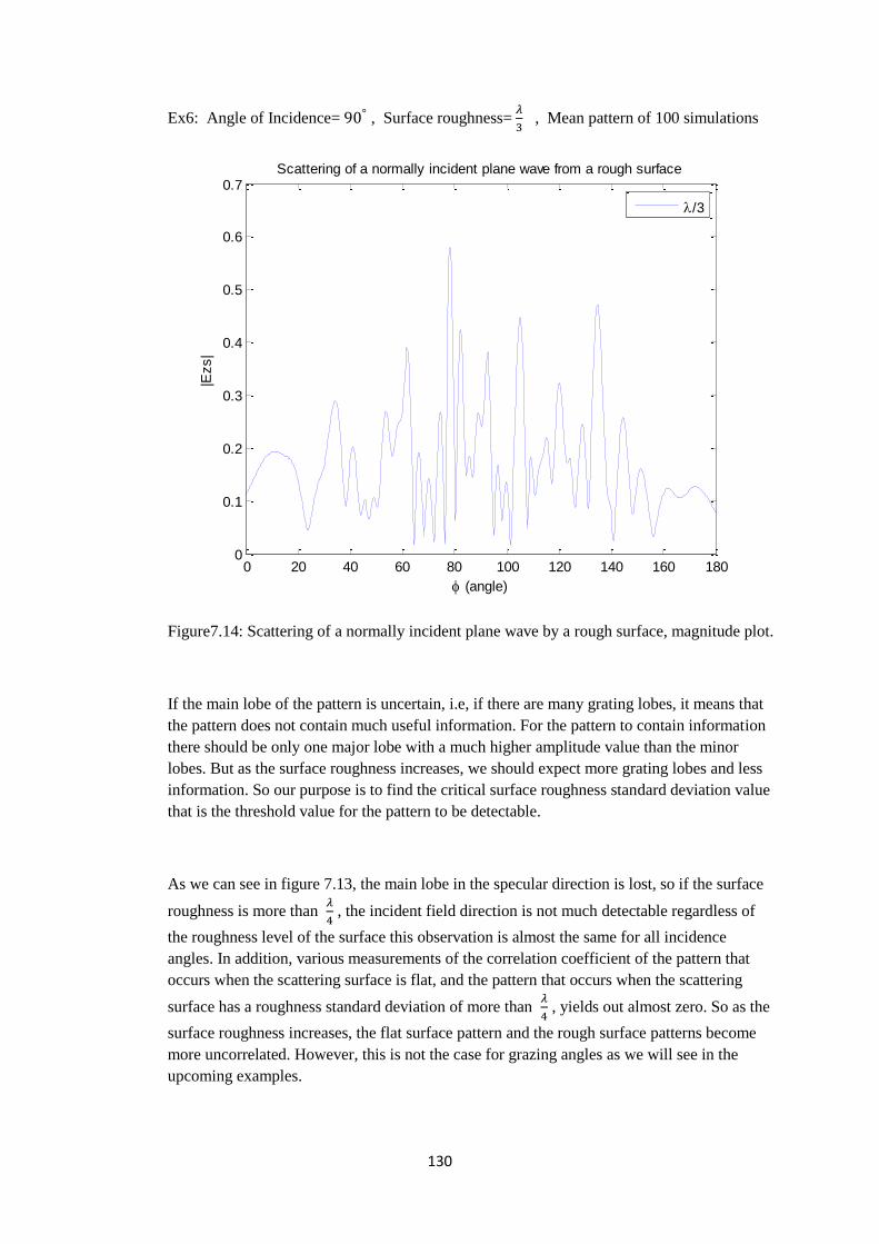
130
Ex6: Angle of Incidence= , Surface roughness=
, Mean pattern of 100 simulations
Figure7.14: Scattering of a normally incident plane wave by a rough surface, magnitude plot.
If the main lobe of the pattern is uncertain, i.e, if there are many grating lobes, it means that
the pattern does not contain much useful information. For the pattern to contain information
there should be only one major lobe with a much higher amplitude value than the minor
lobes. But as the surface roughness increases, we should expect more grating lobes and less
information. So our purpose is to find the critical surface roughness standard deviation value
that is the threshold value for the pattern to be detectable.
As we can see in figure 7.13, the main lobe in the specular direction is lost, so if the surface
roughness is more than
, the incident field direction is not much detectable regardless of
the roughness level of the surface this observation is almost the same for all incidence
angles. In addition, various measurements of the correlation coefficient of the pattern that
occurs when the scattering surface is flat, and the pattern that occurs when the scattering
surface has a roughness standard deviation of more than
, yields out almost zero. So as the
surface roughness increases, the flat surface pattern and the rough surface patterns become
more uncorrelated. However, this is not the case for grazing angles as we will see in the
upcoming examples.
0 20 40 60 80 100 120 140 160 1800
0.1
0.2
0.3
0.4
0.5
0.6
0.7
(angle)
|Ezs|
Scattering of a normally incident plane wave from a rough surface
/3
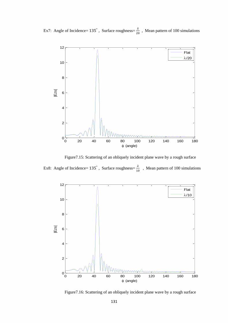
131
Ex7: Angle of Incidence= , Surface roughness=
, Mean pattern of 100 simulations
Figure7.15: Scattering of an obliquely incident plane wave by a rough surface
Ex8: Angle of Incidence= , Surface roughness=
, Mean pattern of 100 simulations
Figure7.16: Scattering of an obliquely incident plane wave by a rough surface
0 20 40 60 80 100 120 140 160 1800
2
4
6
8
10
12
(angle)
|Ezs|
Flat
/20
0 20 40 60 80 100 120 140 160 1800
2
4
6
8
10
12
(angle)
|Ezs
|
Flat
/10
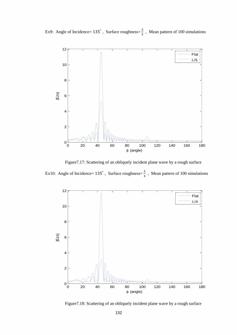
132
Ex9: Angle of Incidence= , Surface roughness=
, Mean pattern of 100 simulations
Figure7.17: Scattering of an obliquely incident plane wave by a rough surface
Ex10: Angle of Incidence= , Surface roughness=
, Mean pattern of 100 simulations
Figure7.18: Scattering of an obliquely incident plane wave by a rough surface
0 20 40 60 80 100 120 140 160 1800
2
4
6
8
10
12
(angle)
|Ezs|
Flat
/5
0 20 40 60 80 100 120 140 160 1800
2
4
6
8
10
12
(angle)
|Ezs|
Flat
/4
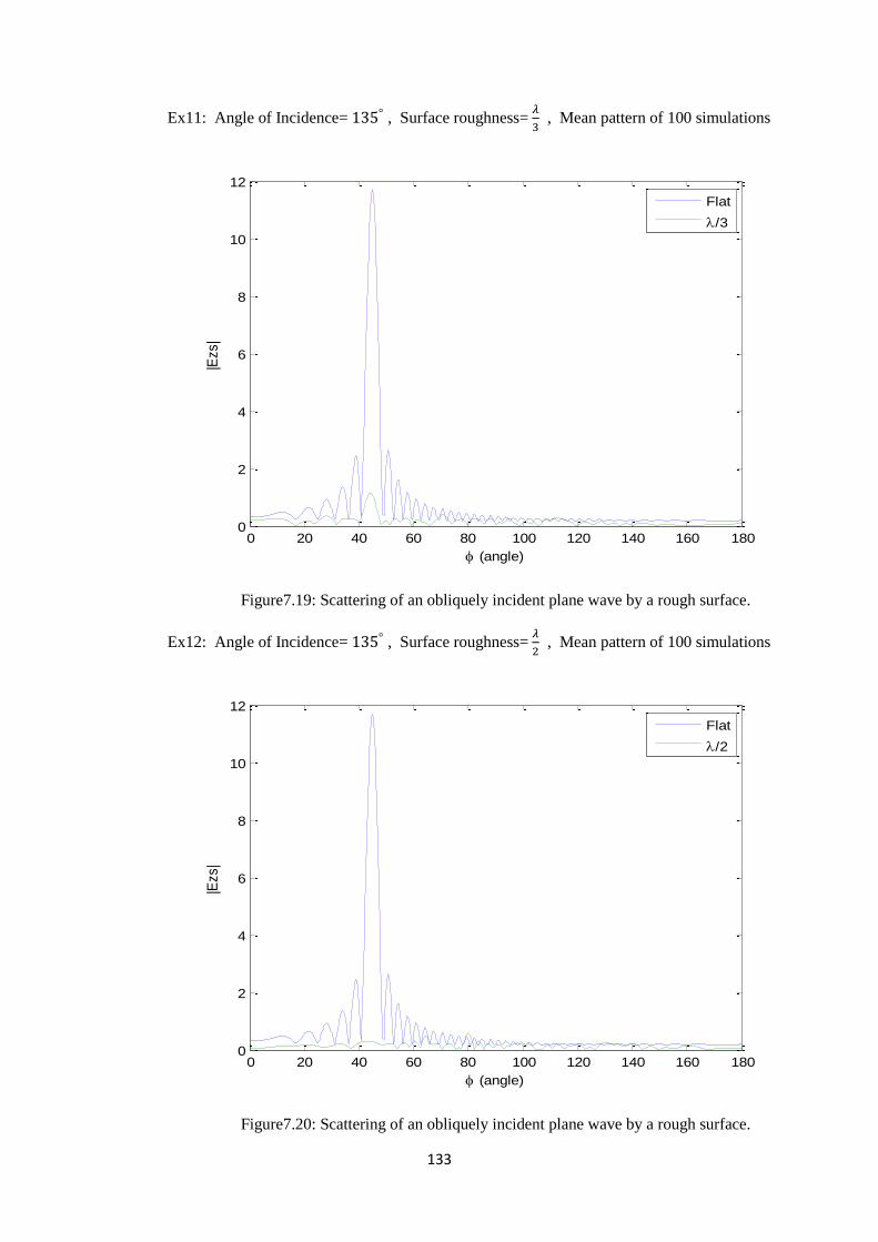
133
Ex11: Angle of Incidence= , Surface roughness=
, Mean pattern of 100 simulations
Figure7.19: Scattering of an obliquely incident plane wave by a rough surface.
Ex12: Angle of Incidence= , Surface roughness=
, Mean pattern of 100 simulations
Figure7.20: Scattering of an obliquely incident plane wave by a rough surface.
0 20 40 60 80 100 120 140 160 1800
2
4
6
8
10
12
(angle)
|Ezs|
Flat
/3
0 20 40 60 80 100 120 140 160 1800
2
4
6
8
10
12
(angle)
|Ezs|
Flat
/2
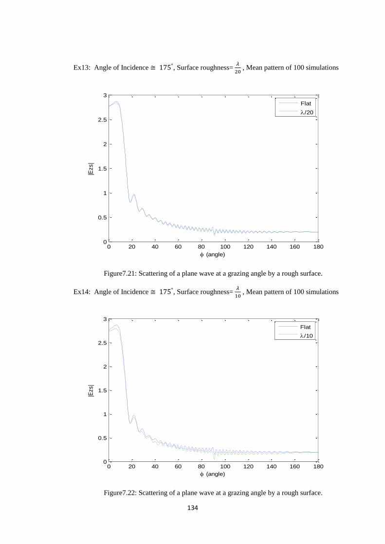
134
Ex13: Angle of Incidence , Surface roughness=
, Mean pattern of 100 simulations
Figure7.21: Scattering of a plane wave at a grazing angle by a rough surface.
Ex14: Angle of Incidence , Surface roughness=
, Mean pattern of 100 simulations
Figure7.22: Scattering of a plane wave at a grazing angle by a rough surface.
0 20 40 60 80 100 120 140 160 1800
0.5
1
1.5
2
2.5
3
(angle)
|Ezs|
Flat
/20
0 20 40 60 80 100 120 140 160 1800
0.5
1
1.5
2
2.5
3
(angle)
|Ezs
|
Flat
/10
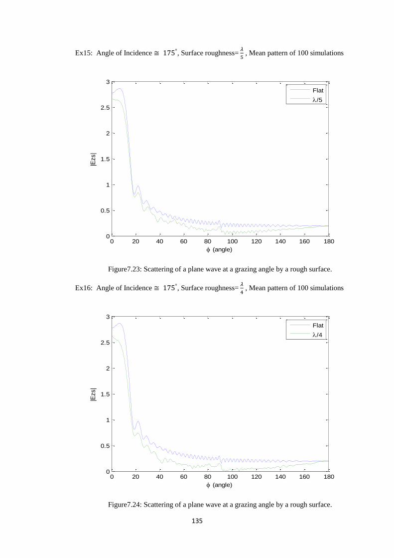
135
Ex15: Angle of Incidence , Surface roughness=
, Mean pattern of 100 simulations
Figure7.23: Scattering of a plane wave at a grazing angle by a rough surface.
Ex16: Angle of Incidence , Surface roughness=
, Mean pattern of 100 simulations
Figure7.24: Scattering of a plane wave at a grazing angle by a rough surface.
0 20 40 60 80 100 120 140 160 1800
0.5
1
1.5
2
2.5
3
(angle)
|Ezs|
Flat
/5
0 20 40 60 80 100 120 140 160 1800
0.5
1
1.5
2
2.5
3
(angle)
|Ezs|
Flat
/4
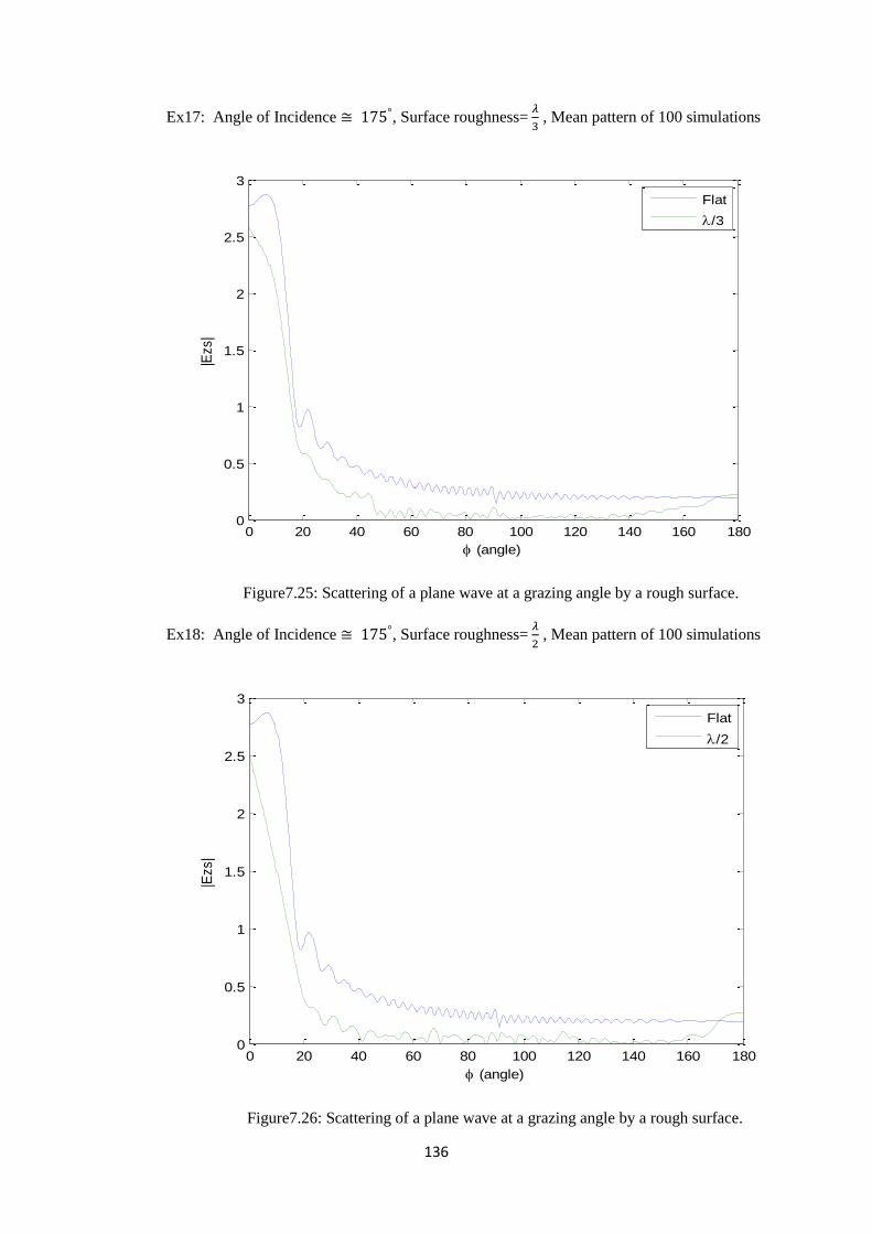
136
Ex17: Angle of Incidence , Surface roughness=
, Mean pattern of 100 simulations
Figure7.25: Scattering of a plane wave at a grazing angle by a rough surface.
Ex18: Angle of Incidence , Surface roughness=
, Mean pattern of 100 simulations
Figure7.26: Scattering of a plane wave at a grazing angle by a rough surface.
0 20 40 60 80 100 120 140 160 1800
0.5
1
1.5
2
2.5
3
(angle)
|Ezs|
Flat
/3
0 20 40 60 80 100 120 140 160 1800
0.5
1
1.5
2
2.5
3
(angle)
|Ezs|
Flat
/2
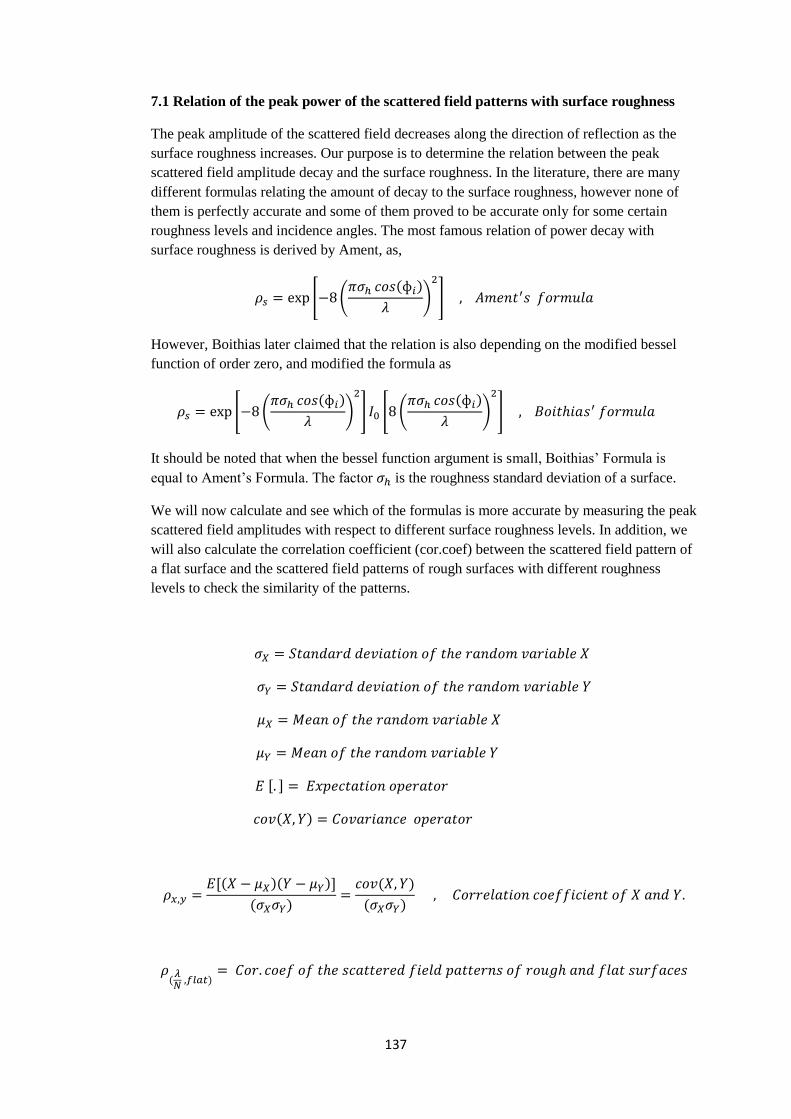
137
7.1 Relation of the peak power of the scattered field patterns with surface roughness
The peak amplitude of the scattered field decreases along the direction of reflection as the
surface roughness increases. Our purpose is to determine the relation between the peak
scattered field amplitude decay and the surface roughness. In the literature, there are many
different formulas relating the amount of decay to the surface roughness, however none of
them is perfectly accurate and some of them proved to be accurate only for some certain
roughness levels and incidence angles. The most famous relation of power decay with
surface roughness is derived by Ament, as,
[ ( ( )
)
]
However, Boithias later claimed that the relation is also depending on the modified bessel
function of order zero, and modified the formula as
[ ( ( )
)
] [ ( ( )
)
]
It should be noted that when the bessel function argument is small, Boithias’ Formula is
equal to Ament’s Formula. The factor is the roughness standard deviation of a surface.
We will now calculate and see which of the formulas is more accurate by measuring the peak
scattered field amplitudes with respect to different surface roughness levels. In addition, we
will also calculate the correlation coefficient (cor.coef) between the scattered field pattern of
a flat surface and the scattered field patterns of rough surfaces with different roughness
levels to check the similarity of the patterns.
[ ]
( )
[( )( )]
( )
( )
( )
(
)
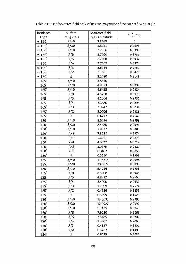
138
Table 7.1:List of scattered field peak values and magnitude of the cor.coef w.r.t angle.
Incidence Angle
Surface Roughness
Scattered field Peak Amplitude
(
)
2.8563 1
2.8321 0.9998
2.7956 0.9993
2.7760 0.9986
2.7308 0.9932
2.7069 0.9874
2.6944 0.9751
2.7161 0.9477
3.2480 0.8148
4.8616 1
4.8073 0.9999
4.6435 0.9984
4.5258 0.9970
4.1064 0.9931
3.6886 0.9895
2.9747 0.9734
2.0006 0.9286
0.4717 0.4647
8.6796 0.9999
8.4580 0.9996
7.8537 0.9982
7.3928 0.9974
5.6561 0.9873
4.3337 0.9714
2.9879 0.9429
0.8482 0.6853
0.5210 0.2399
11.5215 0.9998
10.9627 0.9993
9.4086 0.9953
8.5308 0.9948
4.8232 0.9662
3.4000 0.9430
1.2399 0.7574
0.4556 0.1459
0.3999 0.1525
13.3635 0.9997
12.2927 0.9990
9.7435 0.9940
7.9050 0.9863
3.5485 0.9206
1.3707 0.7063
0.4537 0.3401
0.3767 0.1481
0.6735 0.2035
139
Table7.1 (continued)
Note that (
)
i.e the correlation coefficient of the scattered field patterns of a rough
surface with a roughness standard deviation value of
and a flat surface for a given
incidence angle is actually a complex value. What we are interested in is it’s magnitude
value, therefore it’s magnitude values are given in Table7.1.
In order to see whether the scattered field peak loss fits to the Ament’s Formula or Boithias
formula, we should plot the scattered field peak values versus the standard deviation of
surface roughness for each incidence angle using Table7.1.
It is also important to see the correlation of a rough surface scattered field pattern with that
of a flat surface, given an incidence angle. The correlation coefficient of rough surface
scattered field patterns with a flat surface is expected to decrease as surface roughness
increases. For each incidence angle, we should calculate and plot the correlation coefficient
magnitude of rough surface scattered field patterns with a flat surface, to have a better
understanding of the pattern change with respect to surface roughness.
14.3587 0.9997
12.9495 0.9984
9.3382 0.9921
7.0680 0.9806
2.2844 0.8607
0.9570 0.5119
0.7117 0.0783
0.4327 0.1277
0.6122 0.0460
14.6786 0.9999
13.0730 0.9982
8.9484 0.9921
7.0290 0.9812
2.2409 0.8081
0.7158 0.3398
0.4812 0.1085
0.5383 0.1166
0.7828 0.0754
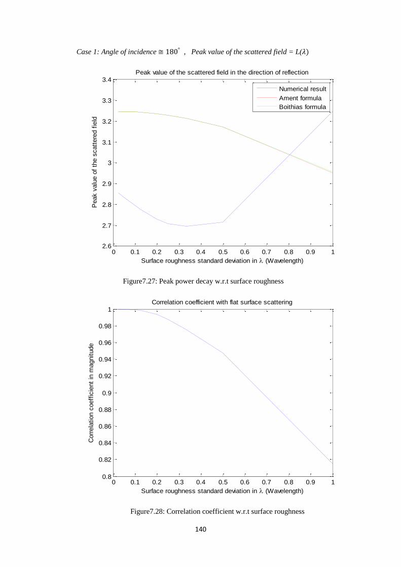
140
Case 1: Angle of incidence , Peak value of the scattered field = L( )
Figure7.27: Peak power decay w.r.t surface roughness
Figure7.28: Correlation coefficient w.r.t surface roughness
0 0.1 0.2 0.3 0.4 0.5 0.6 0.7 0.8 0.9 12.6
2.7
2.8
2.9
3
3.1
3.2
3.3
3.4
Surface roughness standard deviation in (Wavelength)
Peak v
alu
e o
f th
e s
catt
ere
d f
ield
Peak value of the scattered field in the direction of reflection
Numerical result
Ament formula
Boithias formula
0 0.1 0.2 0.3 0.4 0.5 0.6 0.7 0.8 0.9 10.8
0.82
0.84
0.86
0.88
0.9
0.92
0.94
0.96
0.98
1
Surface roughness standard deviation in (Wavelength)
Corr
ela
tion c
oeff
icie
nt
in m
agnitude
Correlation coefficient with flat surface scattering
141
Case 2: Angle of incidence , Peak value of the scattered field = L( )
Figure7.29: Peak power decay w.r.t surface roughness
Figure7.30: Correlation coefficient w.r.t surface roughness
0 0.1 0.2 0.3 0.4 0.5 0.6 0.7 0.8 0.9 10
0.5
1
1.5
2
2.5
3
3.5
4
4.5
5
Surface roughness standard deviation in (Wavelength)
Peak v
alu
e o
f th
e s
catt
ere
d f
ield
Peak value of the scattered field in the direction of reflection
Numerical result, L()
Boithias formula
Ament formula
0 0.1 0.2 0.3 0.4 0.5 0.6 0.7 0.8 0.9 10.4
0.5
0.6
0.7
0.8
0.9
1
Surface roughness standard deviation in (Wavelength)
Corr
ela
tion c
oeff
icie
nt
in m
agnitude
Correlation coefficient with flat surface scattering
142
Case 3: Angle of incidence , Peak value of the scattered field = L( )
Figure7.31: Peak power decay w.r.t surface roughness
Figure7.32: Correlation coefficient w.r.t surface roughness
0 0.1 0.2 0.3 0.4 0.5 0.6 0.7 0.8 0.9 10
1
2
3
4
5
6
7
8
9
Surface roughness standard deviation in (Wavelength)
Peak v
alu
e o
f th
e s
catt
ere
d f
ield
Peak value of the scattered field in the direction of reflection
Numerical result, L()
Boithias formula
Ament formula
0 0.1 0.2 0.3 0.4 0.5 0.6 0.7 0.8 0.9 10.2
0.3
0.4
0.5
0.6
0.7
0.8
0.9
1
Surface roughness standard deviation in (Wavelength)
Corr
ela
tion c
oeff
icie
nt
in m
agnitude
Correlation coefficient with flat surface scattering
143
Case 4: Angle of incidence , Peak value of the scattered field = L( )
Figure7.33: Peak power decay w.r.t surface roughness
Figure7.34: Correlation coefficient w.r.t surface roughness
0 0.1 0.2 0.3 0.4 0.5 0.6 0.7 0.8 0.9 10
2
4
6
8
10
12
Surface roughness standard deviation in (Wavelength)
Peak v
alu
e o
f th
e s
catt
ere
d f
ield
Peak value of the scattered field in the direction of reflection
Numerical result, L()
Boithias formula
Ament formula
0 0.1 0.2 0.3 0.4 0.5 0.6 0.7 0.8 0.9 10.1
0.2
0.3
0.4
0.5
0.6
0.7
0.8
0.9
1
Surface roughness standard deviation in (Wavelength)
Corr
ela
tion c
oeff
icie
nt
in m
agnitude
Correlation coefficient with flat surface scattering
144
Case 5: Angle of incidence , Peak value of the scattered field = L( )
Figure7.35: Peak power decay w.r.t surface roughness
Figure7.36: Correlation coefficient w.r.t surface roughness
0 0.1 0.2 0.3 0.4 0.5 0.6 0.7 0.8 0.9 10
2
4
6
8
10
12
14
Surface roughness standard deviation in (Wavelength)
Peak v
alu
e o
f th
e s
catt
ere
d f
ield
Peak value of the scattered field in the direction of reflection
Numerical result, L()
Boithias formula
Ament formula
0 0.1 0.2 0.3 0.4 0.5 0.6 0.7 0.8 0.9 10.1
0.2
0.3
0.4
0.5
0.6
0.7
0.8
0.9
1
Surface roughness standard deviation in (Wavelength)
Corr
ela
tion c
oeff
icie
nt
in m
agnitude
Correlation coefficient with flat surface scattering
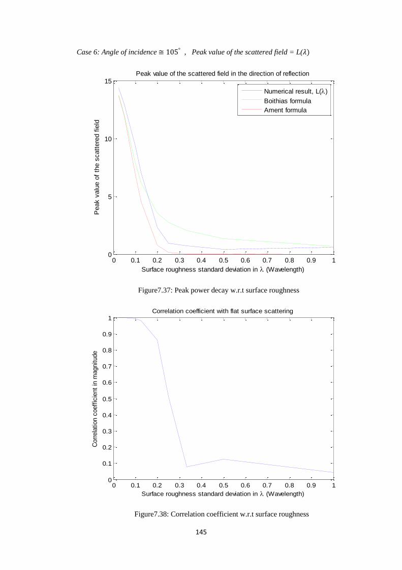
145
Case 6: Angle of incidence , Peak value of the scattered field = L( )
Figure7.37: Peak power decay w.r.t surface roughness
Figure7.38: Correlation coefficient w.r.t surface roughness
0 0.1 0.2 0.3 0.4 0.5 0.6 0.7 0.8 0.9 10
5
10
15
Surface roughness standard deviation in (Wavelength)
Peak v
alu
e o
f th
e s
catt
ere
d f
ield
Peak value of the scattered field in the direction of reflection
Numerical result, L()
Boithias formula
Ament formula
0 0.1 0.2 0.3 0.4 0.5 0.6 0.7 0.8 0.9 10
0.1
0.2
0.3
0.4
0.5
0.6
0.7
0.8
0.9
1
Surface roughness standard deviation in (Wavelength)
Corr
ela
tion c
oeff
icie
nt
in m
agnitude
Correlation coefficient with flat surface scattering
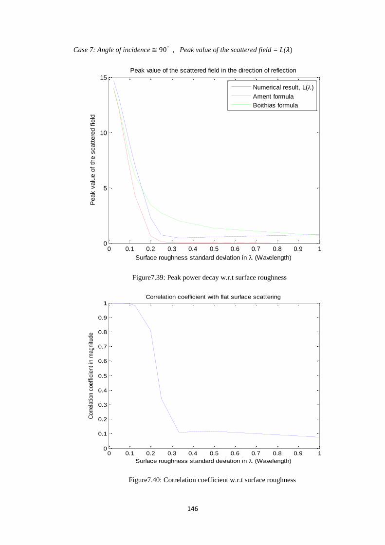
146
Case 7: Angle of incidence , Peak value of the scattered field = L( )
Figure7.39: Peak power decay w.r.t surface roughness
Figure7.40: Correlation coefficient w.r.t surface roughness
0 0.1 0.2 0.3 0.4 0.5 0.6 0.7 0.8 0.9 10
5
10
15
Surface roughness standard deviation in (Wavelength)
Peak v
alu
e o
f th
e s
catt
ere
d f
ield
Peak value of the scattered field in the direction of reflection
Numerical result, L()
Ament formula
Boithias formula
0 0.1 0.2 0.3 0.4 0.5 0.6 0.7 0.8 0.9 10
0.1
0.2
0.3
0.4
0.5
0.6
0.7
0.8
0.9
1
Surface roughness standard deviation in (Wavelength)
Corr
ela
tion c
oeff
icie
nt
in m
agnitu
de
Correlation coefficient with flat surface scattering
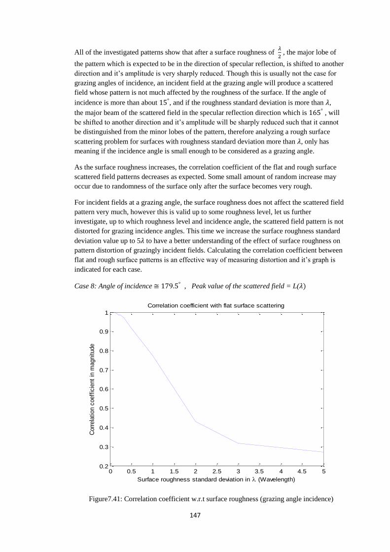
147
All of the investigated patterns show that after a surface roughness of
, the major lobe of
the pattern which is expected to be in the direction of specular reflection, is shifted to another
direction and it’s amplitude is very sharply reduced. Though this is usually not the case for
grazing angles of incidence, an incident field at the grazing angle will produce a scattered
field whose pattern is not much affected by the roughness of the surface. If the angle of
incidence is more than about , and if the roughness standard deviation is more than ,
the major beam of the scattered field in the specular reflection direction which is , will
be shifted to another direction and it’s amplitude will be sharply reduced such that it cannot
be distinguished from the minor lobes of the pattern, therefore analyzing a rough surface
scattering problem for surfaces with roughness standard deviation more than , only has
meaning if the incidence angle is small enough to be considered as a grazing angle.
As the surface roughness increases, the correlation coefficient of the flat and rough surface
scattered field patterns decreases as expected. Some small amount of random increase may
occur due to randomness of the surface only after the surface becomes very rough.
For incident fields at a grazing angle, the surface roughness does not affect the scattered field
pattern very much, however this is valid up to some roughness level, let us further
investigate, up to which roughness level and incidence angle, the scattered field pattern is not
distorted for grazing incidence angles. This time we increase the surface roughness standard
deviation value up to 5 to have a better understanding of the effect of surface roughness on
pattern distortion of grazingly incident fields. Calculating the correlation coefficient between
flat and rough surface patterns is an effective way of measuring distortion and it’s graph is
indicated for each case.
Case 8: Angle of incidence , Peak value of the scattered field = L( )
Figure7.41: Correlation coefficient w.r.t surface roughness (grazing angle incidence)
0 0.5 1 1.5 2 2.5 3 3.5 4 4.5 50.2
0.3
0.4
0.5
0.6
0.7
0.8
0.9
1
Surface roughness standard deviation in (Wavelength)
Corr
ela
tion c
oeff
icie
nt
in m
agnitude
Correlation coefficient with flat surface scattering
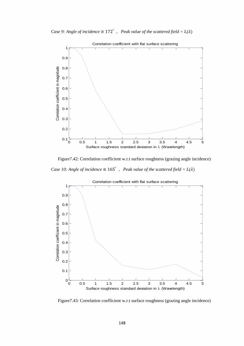
148
Case 9: Angle of incidence , Peak value of the scattered field = L( )
Figure7.42: Correlation coefficient w.r.t surface roughness (grazing angle incidence)
Case 10: Angle of incidence , Peak value of the scattered field = L( )
Figure7.43: Correlation coefficient w.r.t surface roughness (grazing angle incidence)
0 0.5 1 1.5 2 2.5 3 3.5 4 4.5 50.1
0.2
0.3
0.4
0.5
0.6
0.7
0.8
0.9
1
Surface roughness standard deviation in (Wavelength)
Cor
rela
tion
coef
ficie
nt in
mag
nitu
de
Correlation coefficient with flat surface scattering
0 0.5 1 1.5 2 2.5 3 3.5 4 4.5 50
0.1
0.2
0.3
0.4
0.5
0.6
0.7
0.8
0.9
1
Surface roughness standard deviation in (Wavelength)
Corr
ela
tion c
oeff
icie
nt
in m
agnitude
Correlation coefficient with flat surface scattering
149
The Boithias’ formula seems a little more accurate than Ament’s formula for
, but the Ament’s formula is a little more accurate than the Boithias’
formula for , however the two formulas yield different amount of errors
for different angles of incidence, so there is no definite answer of which of them should be
used instead of the other. Usually both formulas yield an accurate result, so either of them
can be used. As the roughness standard deviation value approaches and goes beyond , the
numerical results converges to the Boithias’ formula, however, beyond the rough surface
problem is not worth to investigate as the pattern is almost completely distorted and the
major lobe is lost, this can be verified by checking the correlation coefficient with the pattern
of a flat surface. Therefore convergence of the numerical results to the Boithias’ formula
does not have much importance for us.
Summary:
- As the surface roughness increases the peak value of the pattern’s major lobe is reduced.
- A rough surface scattered field pattern is usually completely distorted after a roughness
standard deviation value of . And will not bear much information.
-Usually both the Ament’s formula and the Boithias’ formula can be used for approximate
analytical results, their accuracy depends on the angle of incidence and the roughness of
the surface and either of them may yield greater error than the other depending on the
surface roughness and the angle of incidence.
- Correlation coefficients of rough surface scattered field patterns with that of a flat surface
scattered field pattern, both at a specific incidence angle, can be calculated to check the
distortion in the rough surface scattered field pattern. Usually a correlation coefficient
below 0.3 means that the pattern is completely distorted, and a correlation coefficient value
below 0.45 means that the pattern is seriously distorted. Above a correlation coefficient
value of 0.7 there is not a serious distortion in the pattern.
-When the incident wave comes at a grazing angle, the scattered field pattern will not be
significantly affected from the roughness of the surface, unless the change in surface
roughness is large.
150
CHAPTER 8
CONCLUSION
The roughness of a given surface has a significant effect on the far field pattern of the
scattered field. As the surface roughness increases, the scattered field pattern becomes more
distorted. For small surface roughness values, the shape of the scattered field pattern is not
affected considerably but the peak value of the pattern experiences a considerable decrease.
For higher levels of surface roughness, the scattered field pattern is almost completely
distorted and the actual major lobe of the pattern that exists for the flat surface scattering
case is totally diminished. It is important to determine the critical roughness levels for each
incidence angle that causes complete distortion in the pattern. We have done this job in the
last chapter and tabulated the results for different roughness levels and for each incidence
angle. This table can be expanded with the expansion of surface roughness values and
incidence angle values into a much greater set of values. But the included results in this
thesis is enough to give a valuable insight to the reader about the topic.
All of the results obtained in chapter 7 are the mean results of 100 different measurements.
Large number of measurements is necessary to provide certainty since the rough surfaces are
all randomly generated. The certainty obtained in the results is a direct consequence of the
central limit theorem. We should find the mean pattern of many different scattered field
patterns in the far field to increase accuracy in measurements.
As the surface roughness increases, the peak value of the scattered field pattern decreases.
This relation was already proven and analyzed by Ament and Boithias, but their useful
mathematical formulations about this relation were not exact and can be erroneous for some
angles of incidence. In this thesis we have checked the accuracy of these formulations and
we have stated our own computed values. Our results are compared with these two formulas.
Based on the results and figures given in chapter 7, it is not clear to say whether Ament’s
formula or Boithias’ formula is more accurate. Both of them become more accurate with
respect to each other for different angles of incidence and for different surface roughness
values. In general, both of the formulas yield accurate results for lower surface roughness
values. However when the standard deviation value of the surface roughness becomes
comparable to the wavelength, the accuracy of these two formulas may decrease and their
accuracy can be examined with the numerical results given in this thesis. There is no point in
comparing the two formulas for surface roughness standard deviation values of more than a
wavelength (λ) as the scattered field pattern becomes completely distorted for such
roughness levels and bears almost no information.
For the grazing angle incidence case, the scattered field pattern is not much affected by the
roughness of the surface up to a standard deviation value of surface roughness of λ .
Above this level of roughness however, the scattered field pattern starts to distort and for
roughness standard deviation values of 2λ or 3λ, the pattern becomes almost completely
151
distorted. For the grazing angle incidence case, the distortion rate is the smallest. The
distortion rate is the largest in the normal incidence case. The table given in chapter 7
indicates the amount of distortion for each roughness level in the grazing angle case and for
other cases as well.
The Ament’s formula and the Boithias’ formula are both not very accurate for the grazing
angle incidence case and the scattered field pattern is not very much affected by the surface
roughness for the grazing angle incidence case. The case of grazing angle incidence can be
seperately investigated in detail in the future.
As a measure of distortion in the scattered field pattern we have used the correlation
coefficient of a rough surface scattered field pattern with a flat surface scattered field pattern.
For different surface roughness values, we have checked the correlation coefficient value and
we have concluded that above a correlation coefficient value of 0.7 the pattern is not
seriously distorted. But a correlation coefficient value below 0.45 indicates a serious
distortion in the scattered field pattern. If the correlation coefficient value is above 0.5, then
the major lobe of the scattered field pattern and the angle of incidence is usually detectable.
If the correlation coefficient value is below 0.35, then the major lobe of the scattered field
pattern and the angle of incidence is usually not detectable. Measuring the correlation
coefficient of rough and flat surface scattered field patterns is a useful and accurate method
for checking pattern distortion. But some other methods may also be used to measure far
field pattern distortion.

152
REFERENCES
[1] Constantine A.Balanis, Advanced Engineering Electromagnetics,1989 edition, by John
Wiley & Sons, pages 2-120.
[2] Jean Pierre Berenger, A Perfectly Matched Layer For The Absorption Of
Electromagnetic Waves, Journal Of Computational Physics 114 (1994), pages 185-200.
[3] http://www.mathworks.com/help/pde/index.html , MATLAB Partial Differential
Equation (PDE) Toolbox, last accessed date: 21 December 2012.
[4] http://en.wikipedia.org/wiki/Normal_distribution , last accessed date 14 December
2012.
[5] Matthew N.O.Sadiku, Numerical Techniques In Electromagnetics With MATLAB,
Third Edition, pages 235-245 and 379-435.
[6] Ozlem Ozgun, Mustafa Kuzuoglu, Near-field performance analysis of locally-
conformal perfectly matched absorbers via Monte Carlo simulations, Journal of
Computational Physics, vol. 227, no. 2, pp. 1225-1245, 2007.
[7] Shree K.Nayar, Katsushi Ikeuchi, Takeo Kanade, Surface Reflection: Physical and
Geometrical Perspectives, IEEE Transactions on pattern analysis and machine intelligence,
vol. 13, no. 7, July 1991.
[8] J. N.Reddy, An Introduction To The Finite Element Method, Mc Graw –Hill
International Editions, Mathematics and Statistics Series (1984) , pages 194-220.
[9] Jin Au Kong, Electromagnetic Wave Theory (1986) , Chapters 1-2.
[10] Kevin Krause, Application Of The Finite Element Method To Random Rough Surface
Scattering With Neumann Boundary Conditions, MSc. Thesis, University Of Washington,
pages 1-13.
[11] Simon N. Chandler-Wilde, Peter Monk, The PML For Rough Surface Scattering,
ScienceDirect Applied Numerical Mathematics, Applied Numerical Mathematics 59
(2009) 2131-2154, www.elsevier.com/locate/apnum
[12] N.C Bruce, J.C Danity, Multiple scattering from random rough surfaces using the
Kirchoff approximation, Journal of modern optics, 1991, vol. 38, no. 3, pp. 579-590 .
[13] Ozlem Ozgun, Mustafa Kuzuoglu, Monte Carlo –Based Characteristic Basis Finite-
Element Method for Numerical Analysis of Scattering From Objects On/Above Rough Sea
Surfaces, IEEE Transactions on GeoScience and Remote Sensing, vol. 50, no. 3, pp. 769-
783, 2012.