VARIATIONAL APPROACH TO SCATTERING BY UNBOUNDED ROUGH ...€¦ · VARIATIONAL APPROACH TO SCATTERING BY UNBOUNDED ROUGH SURFACES WITH NEUMANN AND GENERALIZED IMPEDANCE BOUNDARY

COMMUN. MATH. SCI. c© 2015 International Press

Vol. 13, No. 2, pp. 511–537

VARIATIONAL APPROACH TO SCATTERING BY UNBOUNDEDROUGH SURFACES WITH NEUMANN AND GENERALIZED

IMPEDANCE BOUNDARY CONDITIONS∗

GUANGHUI HU† , XIAODONG LIU‡ , FENGLONG QU§ , AND BO ZHANG¶

Abstract. This paper is concerned with problems of scattering of time-harmonic electromagneticand acoustic waves from an infinite penetrable medium with a finite height modeled by the Helmholtzequation. On the lower boundary of the rough layer, the Neumann or generalized impedance boundarycondition is imposed. The scattered field in the unbounded homogeneous medium is required to satisfythe upward angular-spectrum representation. Using the variational approach, we prove uniquenessand existence of solutions in the standard space of finite energy for inhomogeneous source terms, andin appropriate weighted Sobolev spaces for incident point source waves in Rm (m= 2,3) and incidentplane waves in R2. To avoid guided waves, we assume that the penetrable medium satisfies certainnon-trapping and geometric conditions.

Key words. Rough surface scattering, Helmholtz equation, generalized impedance boundarycondition, Neumann boundary condition, angular-spectrum representation, uniqueness and existence,weighted Sobolev space.

AMS subject classifications. 35J05, 35J20, 35J25, 42B10, 78A45.

1. IntroductionThis paper is concerned with the mathematical analysis of problems of scattering of

time-harmonic electromagnetic and acoustic waves from an infinite and inhomogeneousmedium of a finite height governed by the Helmholtz equation. The interface betweenthe finite inhomogeneous layer and the unbounded homogeneous medium is supposedto be a rough surface, which usually means a non-local perturbation of an infinite planesurface such that the surface lies within a finite distance of the original plane. Suchscattering problems have been of interest to physicists, engineers and applied mathe-maticians for many years due to their wide range of applications in optics, acoustics,radio-wave propagation, seismology and radar techniques (see, e.g., [2, 3, 28, 30]).

There has been already a vast literature on rough surface scattering problems foracoustic and electromagnetic waves. We refer the reader to [6, 7, 10, 11, 12, 32] and[29, Chapter 5] for the integral equation method applied to the Dirichlet or impedanceboundary value problem with smooth (C1,α) surfaces in Rm (m= 2,3) and to [13, 31] forscattering by penetrable interfaces and inhomogeneous layers. The variational approachproposed in [8] by Chandler-Wilde and Monk gives rise to existence and uniquenessresults in non-weighted Sobolev spaces, allowing to treat the scattering problem due toan inhomogeneous source term whose support lies within a finite distance above rathergeneral sound-soft surfaces in Rm (m= 2,3). Moreover, this approach leads to explicitbounds on solutions in terms of the data and applies to acoustic scattering by impedancesurfaces, by inhomogeneous rough layers as well as by penetrable interfaces; see, e.g.,

∗Received: January 25, 2014; accepted (in revised form): May 15, 2014. Communicated by OlofRunborg.†Weierstrass Institute for Applied Analysis and Stochastics, Mohrenstr. 39, 10117 Berlin, Germany

([email protected]).‡Institute of Applied Mathematics, AMSS, Chinese Academy of Sciences, Beijing 100190, P.R. China

([email protected]).§School of Mathematics and Information Science, Yantai University, Yantai 264005, Shandong, P.R.

China ([email protected]).¶LSEC and Institute of Applied Mathematics, AMSS, Chinese Academy of Sciences, Beijing 100190,

P.R. China ([email protected]).

511

512 SCATTERING BY UNBOUNDED ROUGH SURFACES

[9, 24, 29, 26]. A recently developed variational approach in weighted Sobolev spacescovers the plane wave incidence case for two-dimensional sound-soft rough surfaces,whereas in the 3D case incident spherical and cylindrical waves can be treated; seeChandler-Wilde & Elschner [5]. Recently, the variational approach developed in [8] and[5] has been extended to the electromagnetic and elastic cases in [18, 19, 21, 25]. Otherstudies [14, 15] have been carried out by Duran, Muga, and Nedelec for treating surfacewaves arising from locally perturbed impedance rough surfaces, where the sign of theimpedance coefficient is the opposite of ours.

The aim of this paper is to investigate the rough surface scattering problems withthe Neumann boundary condition (NBC) and the Generalized Impedance BoundaryCondition (GIBC). These boundary conditions have important applications in the realworld. For example, GIBC models the third-order approximation of electromagneticscattering by highly conducting materials, while the Neumann boundary condition isthe exactly the zero-order approximation in the case of transverse magnetic (TM) po-larization (see, e.g., [16, 22, 23] and the references therein). Using variational approach,we prove existence and uniqueness of solutions at arbitrary frequency for the scatteringproblem due to either an inhomogeneous source term, an incident point source wave inRm (m= 2,3), or an incident plane wave in R2. The refractive index characterizing theinhomogeneous medium is required to satisfy a certain non-trapping condition in orderto exclude guided waves. For the Neumann boundary value problem, we assume thatthe upper boundary of the inhomogeneous medium is a Lipschitz graph but the lowerboundary is a flat plane, which means that the inhomogeneous medium is sitting on ahalf space; see Figure 4.1.

Our method is closest to the variational approach of Chandler-Wilde and Monk[8] in a non-weighted setting and that of Chandler-Wilde and Elschner [5] in weightedSobolev spaces. We have employed several new ideas from electromagnetic and elasticwave scattering problems [18, 21]. Compared with the earlier work, the novel contri-butions of the present study are summarized as follows. (i) We present a shorter andsimpler proof of the well-posedness of acoustic scattering from generalized impedancerough surfaces given by Lipschitz graphs. Instead of the generalized Lax-Milgram lemmaused for the classical impedance rough surfaces (see [29]), our proof is based on a pertur-bation argument for semi-Fredholm operators in combination with the well-posedness ofthe Dirichlet problem. This idea stems from [18, Lemma 5.2], where the Lame equationis treated in the non-weighted space and from [20, Lemma 7] on the a priori estimate forsolutions of the Helmholtz equation in periodic structures. The proof applies straight-forwardly to the classical impedance boundary conditions, provided the rough surface isa Lipschitz graph. (ii) In the Neumann case, we have imposed a rather general condition(see condition (iii) in Theorem 4.1) relating the refractive index with the transmissioncoefficient, which covers both the TE and TM transmission conditions. The approachdealing with the transmission conditions extends directly to the rough surface scatter-ing problems in the whole space. Since a piecewise constant refractive index satisfiesthe non-decreasing condition, our non-trapping condition is more general than that em-ployed in [21] for the full Maxwell system. Note that the Neumann surface is requiredto be flat since we could obtain vanishing boundary terms over the surface (see (4.14))in deriving the a priori estimate via the Rellich identities. This trick was already usedin [21] for treating the electromagnetic scattering from penetrable dielectric layers lyingon a perfect conductor in a half space; see also [31], where the TM polarization casewas studied using the integral equation method. (iii) We have derived wave number-explicit bounds on the solution for inhomogeneous source terms (see theorems 3.4 and

G. HU, X. LIU, F. QU, AND B. ZHANG 513

4.1), which might be important to numerical analysis. The dependence of the boundson the Lipschitz constant of the rough interface is also obtained.

Here, we mention several features of our paper. Unlike [5], our variational equationsfor incident plane waves are formulated in a straightforward way, with the right-handside explicitly expressed in terms of the plane wave. As shown in [5], one can readilyjustify the quasi-periodicity of solutions when the medium is periodic and the incidentwave is quasi-periodic. The proof for the Neumann boundary value problem (NBVP)slightly differs from the Generalized Impedance Boundary value Problem (GIBVP),and thus we have presented exactly two different ways in the framework of functionalanalysis for treating rough surface scattering problems; cf. lemmas 3.1 and 4.2. Bothapproaches rely crucially on the a priori estimate of solutions to the Helmholtz equationat arbitrary wave numbers.

The rest of the paper is organized as follows. In Section 2, we rigorously formulatethe GIBVP for the wave scattering due to an inhomogeneous source term, and proposethe equivalent variational formulation in the usual Sobolev space with finite energy.The uniqueness and existence proofs will be carried out in Section 3, based on theabstract functional analysis described in Lemma 3.1. Section 4 is devoted to the uniquesolvability of the NBVP under certain assumptions. The final Section 5 deals with thewell-posedness in weighted Sobolev spaces for incident plane and point source waves.

2. The GIBVP and its variational formulationConsider the time-harmonic electromagnetic scattering (with time variation of the

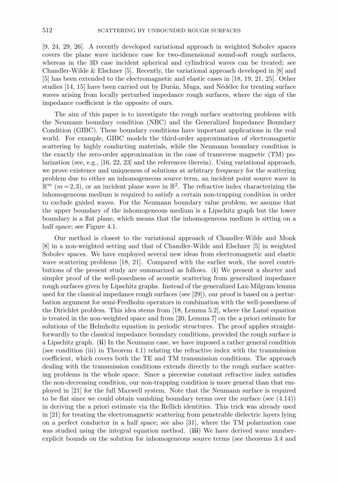
form exp(−iωt), ω>0) due to a source term g in an infinite inhomogeneous layer offinite height lying above an imperfect conductor with a high conductivity. For x=(x1,. ..,xm)∈Rm (m= 2,3), let x= (x1,. ..,xm−1) so that x= (x,xm). For H ∈R, letUH =x :xm>H and ΓH =x :xm=H. Let D⊂Rm be a connected open set suchthat for some constants f−<f+ it holds that

Uf+ ⊂D⊂Uf− .

Fig. 2.1. The geometric settings for GIBVP. For x= (x,xm)∈Rm, Γ =x :xm =f(x), Uf+ =

x :xm>f+, D=x :xm>f(x). A GIBC is imposed on Γ.

Denote by Rm\D the imperfect conductor with a high conductivity under consideration.Throughout the paper, it is supposed that the boundary Γ :=∂D of D is given by the


graph of a bounded and uniformly Lipschitz continuous function f , i.e.,

Γ :=xm=f(x),x∈Rm−1, |f(x)−f(y)|≤L|x− y|, ∀ x, y∈Rm−1, (2.1)

with the Lipschitz constant L>0; see Figure 2.1. In the TE polarization case, theelectromagnetic scattering problem can be modeled by the inhomogeneous Helmholtzequation

∆u+k2n(x)u=g in D, (2.2)

in a distributional sense, with the positive constant wave number given by k :=√µ0ε0ω

in terms of the electric permittivity ε0>0 and the magnetic permeability µ0>0 inthe vacuum. The refractive index function n(x), which models the medium inside theinhomogeneous layer D\Uf+ , is given by

n(x) =

1 in Uf+ ,ε(x)

ε0+ i

σ(x)

ωε0in D\Uf+ ,

i=√−1, (2.3)

where the electric permittivity ε(x)>0 and the conductivity σ(x)>0 are both spatiallyvarying functions. Since Rm\D consists of highly conducting materials, there is a rapidexponential decay of the wave inside Rm\D, i.e., the electromagnetic field cannot pene-trate deeply into Rm\D. The scattering effect on Γ in this case can be modeled by thegeneralized impedance boundary condition

∂u

∂ν+divΓ(µ∇Γu)+λu= 0 on Γ, (2.4)

where ν= (ν1,·· · ,νm) stands for the unit norm pointing into D, and divΓ and ∇Γ arerespectively the surface divergence and the surface gradient on Γ. We refer to [22]for the associated asymptotic analysis and error estimate for scattering problems fromunbounded highly absorbing media. If µ= 0, (2.4) reduces to the standard impedanceboundary condition which corresponds to the second-order approximation of the electro-magnetic scattering by highly conducting materials. The generalized impedance bound-ary condition (2.4) is exactly the third-order approximation of the scattering problem,and thus could lead to more precise and accuracy reflecting effects.

In this paper, we assume that the impedance coefficients λ and µ are constantssatisfying

Re(λ)≤0, Im(λ)>0, Im(µ)≤0, Re(µ)>0. (2.5)

The differential operator divΓ(µ∇Γ·) can be interpreted as follows. For v∈H1(∂D) thesurface gradient ∇Γv lies in the tangential space L2

t (Γ) :=V ∈L2(∂D) :ν ·V = 0. Theoperator divΓ(µ∇Γu) is defined in H−1(Γ) by⟨

divΓ(µ∇Γu),v⟩

=−∫

Γ

µ∇Γu ·∇Γvds, ∀v∈H1(∂D),

where⟨·,·⟩

stands for the duality pairing in⟨H−1(Γ),H1(Γ)

⟩which is an extension of

the inner product in L2(Γ).The variational problem will be posed on the open set SH =D\UH for some H>f+.

To derive an equivalent variational formulation, we adapt the upward Angular SpectrumRepresentation proposed in [8], which can be written as

u(x) =1

(2π)(m−1)/2

∫Rm−1

exp(i[(xm−H)√k2−ξ2 + x ·ξ])FH(ξ)dξ, x∈UH , (2.6)


where FH =u|ΓHand FH =FFH denotes the Fourier transform of FH given by

Fv=1

(2π)(m−1)/2

∫Rm−1

exp(−ix ·ξ)v(x)dx, m= 2,3.

In this equation,√k2−ξ2 = i

√ξ2−k2 when ξ2>k2. The representation of u in the

integral (2.6) can be interpreted as a formal radiation condition in the physics andengineering literature on rough surface scattering (see e.g. [28]). We will discuss theGIBVP due to the source term in the Hilbert space

VH :=φ|SH:φ∈H1(D),φ∈H1(Γ), H≥f+,

equipped with the norm

‖|u‖|VH:=‖u‖H1(SH) +‖u‖H1(Γ), (2.7)

where H1(·) denotes the standard Sobolev space. By the trace lemma, we have FH ,FH ∈L2(Γ), and thus the right hand side of (2.6) makes sense for every x∈UH . Whenu|ΓH

∈BC(ΓH)∩L∞(ΓH), the space of bounded and continuous functions on ΓH , ithas been shown in [1] by Arens and Hohage that (2.6) can be interpreted as a bilineardual pairing of H−s and Hs with 1/2<s<1 in two dimensions.

We emphasize that in this paper, unless otherwise stated, we employ the equivalentnorm ‖·‖VH

to ‖| ·‖| (see (2.7)) given by

‖u‖2VH:=

∫SH

(|∇u|2 +k2|u|2)dx+Im(λ)‖u‖2L2(Γ) +Re(µ)‖∇Γu‖2L2(Γ),

which depends on the wave number k2 and the impedance coefficients λ and µ.The generalized impedance boundary value problem can be stated as follows.

(GIBVP) : Given g∈L2(D) whose support lies in SH , determine u :D→C such thatu|SH

∈VH satisfies the equation (2.3) in a distributional sense, the boundarycondition (2.4) in a weak sense and the Angular Spectrum Representation (2.6).

We will prove the existence and uniqueness of solutions to (GIBVP) under thefollowing non-trapping condition

(A): n∈L∞(D) and Re[n(x)] is monotonically increasing as xm increases, that is,

essinf[Re[n(x+sem)−n(x)

]:x∈D

]≥0 (2.8)

for all s>0, where em denotes the m-th Cartesian unit vector of Rm.

Obviously, under the assumption (A) we have the upper bound

||Re(n)||L∞(D)≤1. (2.9)

The condition (2.8) can be slightly relaxed; see Remark 3.1 at the end of the nextsection.

The variational formulation of (GIBVP). In the following, we will introducesome trace operators and a Dirichlet-to-Neumann operator defined on ΓH . To de-scribe the mapping properties of these operators we use standard fractional Sobolevspace notation equipped with a wave number dependent norm that is equivalent to the


usual norm. Identifying ΓH with Rm−1, we denote by Hs(ΓH), s∈R the completion ofC∞0 (ΓH) endowed with the norm

‖φ‖Hs(ΓH) =

(∫Rm−1

(k2 + |ξ|2

)s |Fφ(ξ)|2dξ)1/2

. (2.10)

We recall [8] that, for all a>H>f+ there exist continuous embeddings γ+ :H1(UH\Ua)→H1/2(ΓH) and γ− :VH→H1/2(ΓH) such that γ±φ coincides with the re-striction of φ to ΓH when φ∈C∞. It is also known that, if u+∈H1(UH\Ua), u−∈VH ,and γ+u+ =γ−u−, then v∈Va, where v(x) :=u+(x), x∈UH\Ua, :=u−(x), x∈SH . Con-versely, if v∈Va and u+ :=v|UH\Ua

, u− :=v|SH, then γ+u+ =γ−u−.

The Dirichlet-to-Neumann (DtN) operator T is defined by

T =T (k) :=F−1MzF , (2.11)

where Mz =Mz(k) is the operator of multiplying by

z(ξ;k) :=

−i√k2−|ξ|2 if |ξ|≤k,√|ξ|2−k2 if |ξ|>k.

Hence, it follows that, if FH ∈C∞0 (ΓH) and u is defined by (2.6), then

Tγ+u=− ∂u

∂xm|ΓH

. (2.12)

Let us recall two lemmas which concern properties of the DtN operator T .

Lemma 2.1. ([8])

(i) The DtN operator T :H1/2(ΓH)→H−1/2(ΓH) is bounded with the norm‖T‖H1/2(ΓH)→H−1/2(ΓH) = 1.

(ii) For all φ,ψ∈H1/2(ΓH), we have∫ΓH

φTψds=

∫ΓH

ψTφds.

For all φ∈H1/2(ΓH), it holds that

Re

∫ΓH

φTφds≥0 and Im

∫ΓH

φTφds≤0.

The following lemma describes properties of u, defined by (2.6) (see [8]).

Lemma 2.2. If (2.6) holds with FH ∈H1/2(ΓH), then u∈H1(UH\Ua)∩C2(UH) forevery a>H,

4u+k2u= 0 inUH ,

γ+u=FH , and∫ΓH

γ+vTγ+uds+k2

∫UH

uvdx−∫UH

∇u ·∇vdx= 0, v∈H1(D). (2.13)

Further, the restrictions to Γa of u and ∇u are in L2(Γa) for all a>H, and∫Γa

[ | ∂u∂xm

|2−|∇xu|2 +k2|u|2 ]ds≤2k Im

∫Γa

u∂u

∂xmds. (2.14)


Moreover, for all a>H, (2.6) holds with H replaced by a.

In what follows we shall derive an equivalent variational formulation for (GIBVP),following the spirit of [8], where the Dirichlet boundary value problem was treated. De-fine D(SH) :=v|SH

:v∈C∞0 (Rm), so that D(SH) is dense in H1(SH). Let the traceoperator γ∗ :D(SH)→L2(Γ) be defined by γ∗φ=φ|Γ for φ∈D(SH). Then it can beextended to a bounded linear operator γ∗ :H1(SH)→L2(Γ). Now suppose that u is asolution to (GIBVP), then u|Sa

∈Va for every a>f+. Since u satisfies the inhomoge-neous equation (2.2) and the boundary condition (2.4) in the weak sense, we have∫

D

[gv+∇u ·∇v−k2n(x)uv]dx−∫

Γ

[λγ∗uγ∗v+µ∇Γu ·∇Γv]ds= 0, v∈H1(D).

(2.15)

Defining w :=u|SHand then applying Lemma 2.2, it follows that

0 =

∫SH

[gv+∇w ·∇v−k2n(x)wv]dx+

∫ΓH

γ−vTγ−wds

−∫

Γ

[λγ∗wγ∗v−µ∇Γw ·∇Γv]ds, (2.16)

for v∈H1(D). Let ‖·‖2 and (·, ·) denote the norm and scalar product on L2(SH), thatis,

‖v‖2 =

(∫SH

|v|2dx)1/2

, (w,v) =

∫SH

wvdx.

Define the sesquilinear form b :VH×VH→C by

b(w,v) = (∇w,∇v)−k2(n(x)w,v)+

∫ΓH

γ−vTγ−wds

−∫

Γ

[λγ∗wγ∗v−µ∇Γw ·∇Γv]ds. (2.17)

The form b obviously generates a continuous linear operator B=B(k) :VH→V ∗H suchthat

(Bw,v) = b(w,v), ∀v∈VH , (2.18)

where V ∗H denotes the dual of the space VH with respect to the duality (·,·). Thus,if u is a solution to (GIBVP), then w :=u|SH

is a solution of the following variationalproblem: find w∈VH such that

(Bw,v) =−(g,v) for all v∈VH . (2.19)

Conversely, assume w is a solution to the variational problem (2.19). Introduce thefunction

u(x) :=

w(x), x∈SH ,

the integral (2.6) with FH :=γ−w, x∈UH .

Then, by Lemma 2.2, u∈H1(UH\Ua) for every a>H with γ+u=FH =γ−w. Thus,u|Sa∈Va for all a>f+. Furthermore, by (2.13) and (2.16) it can be shown that (2.15)


holds. Hence, u is a weak solution to GIBVP. The above analysis yields the followinglemma.

Lemma 2.3. If u is a solution of (GIBVP), then u|SHsatisfies the variational problem

(2.19). Conversely, if u satisfies the variational problem (2.19) with FH =γ−u, then theextended solution u to D by setting u(x) as the right-hand side of (2.6) is a solution of(GIBVP), with g extended by zero from SH to D.

3. Unique solvability of (GIBVP)The aim of this section is to prove the uniqueness and existence of solutions to

(GIBVP) by analyzing the operator equation (2.19) for an arbitrary wave number k2>0.Our proof is based on the perturbation of semi-Fredholm operators, shown as follows.

Lemma 3.1 (see [18]). Let X, Y be infinite-dimensional Banach spaces equippedwith norm || · ||X and || · ||Y , and let L(X,Y ) denote by the set of all bounded linearoperators from X to Y . Assume that B(k),k∈R+⊂L(X,Y ), and that B(k) dependscontinuously on the parameter k in the operator norm. Suppose further that

(i) ||B(k)(u)||Y ≥C(k)||u||X for some constant C(k)>0 and each k∈R+;

(ii) there exists a small number k0>0 such that the inverse of B(k) exists for all k∈(0,k0].

Then the operator B(k) is invertible for all k∈R+, with the operator norm of its inversefulfilling the bound ||B(k)−1||Y→X ≤C(k)−1.

To apply Lemma 3.1, we shall take X=VH ,Y =V ∗H , and define B(k) to be the sameas the operator in (2.18). We first check that B(k) indeed depends continuously onk∈R+, i.e.,

||B(k)−B(k1)||VH→V ∗H→0 as k→k1, k,k1∈R+. (3.1)

To prove (3.1), we adapt the wave number-independent norms |||u|||VHgiven in (2.7)

and |||u|||Hs(ΓH) (s∈R) defined analogously to the norm ||u||Hs(ΓH) (see (2.10)) butwith k= 1. By the definitions of T (k) and the norm || · ||Hs , we see

|||T (k)u−T (k1)u|||2H−1/2(ΓH)

=

∫Rm−1

(1+ |ξ|2)−1/2|(Mz(k)−Mz(k1))uH(ξ)|2dξ

≤||u||2H1/2(ΓH) supξ∈Rm−1

|z(ξ;k)−z(ξ;k1)|2

1+ |ξ|2.

Consequently,

||T (k)−T (k1)||H1/2(ΓH)→H−1/2(ΓH)

= sup|||T (k)u−T (k1)u |||H−1/2(ΓH) : |||u |||H1/2(ΓH) = 1

≤

[sup

ξ∈Rm−1

|z(ξ;k)−z(ξ;k1)|2

1+ |ξ|2

]1/2

→0, as k→k1. (3.2)

Hence, the convergence in (3.1) simply follows from the definitions of the operator B(k)and the sesquilinear form b combined with the continuity of the DtN map T in theoperator norm as shown in (3.2). Thus it remains to justify the conditions (i) and (ii) in


Lemma 3.1. The invertibility of the operator B(k) for small wave numbers is presentedin the following lemma.

Lemma 3.2. The sesquilinear form b(·, ·) is coercive over VH for sufficiently smallwave numbers. More precisely, there exists a number k0>0 such that

|(Bw,w)|≥√

2

4‖w‖2VH

, for allk∈ (0,k0].

Hence, the operator B(k) :VH→V ∗H is invertible for all k<k0.

Proof. Taking the real part of the sesquilinear form b(·, ·) in (2.17) with v=w and,making use of Lemma 2.1 and the assumption (2.8), we obtain

Re(Bw,w) =

∫SH

|∇w|2−k2Re[n(x)]|w|2dx+Re

∫ΓH

γ−wTγ−wds

−∫

Γ

[Re(λ)|γ∗w|2−Re(µ) |∇Γw|2

]ds

≥∫SH

|∇w|2−k2|w|2dx+

∫Γ

Re(µ) |∇Γw|2ds. (3.3)

Taking the imaginary part of the sesquilinear form b(·,·) in (2.17), it follows that

Im(Bw,w) =−k2

∫SH

Im[n(x)]|w|2dx+Im

∫ΓH

γ−wTγ−wds

−∫

Γ

[Im(λ)|γ∗w|2− Im(µ) |∇Γw|2

]ds. (3.4)

Using Lemma 2.1 and the fact that Im(n(x))≥0, Im(λ)>0, Im(µ)≤0, we obtain

|Im(Bw,w)|≥ Im(λ)‖w‖2L2(Γ). (3.5)

Combining (3.3) and (3.5) yields

|(Bw,w)|≥√

2/2|Re(Bw,w)|+ |Im(Bw,w)|

≥√

2/2‖∇w‖22−k2‖w‖22 +Re(µ)‖∇Γu‖2L2(Γ) +Im(λ)‖w‖2L2(Γ)

=√

2/2||w||2VH

−2k2||w||22. (3.6)

Recall the estimate (see [29])

‖w‖22≤ (H−f−)2‖ ∂w∂xm

‖22 +2(H−f−)‖w‖2L2(Γ)

≤ (H−f−)2‖∇w‖22 +2(H−f−)‖w‖2L2(Γ). (3.7)

Now, set

k20 = min

1

4(H−f−)2,

Im(λ)

8(H−f−)

.

Then, by (3.7) we have for all k<k0,

2k2‖w‖22≤2k20‖w‖22≤

1

2

[‖∇w‖22 +(Im(λ))‖w‖2L2(Γ)

]≤ 1

2||w||2VH


which, together with (3.6), gives

|(Bw,w)|≥√

2/4 ||w||2VH.

This ends the proof of Lemma 3.2.

In order to apply Lemma 3.1, we need further to check the condition (i), i.e., theinequality

||u||VH≤C ||G||V ∗H , for all u∈VH , G :=B(k)u∈V ∗H , (3.8)

for each k∈R+. Analogously to [8, Lemma 4.5], we reduce the problem of justifying(3.8) to that of proving an a priori bound for solutions of the variational equation (2.19).

Lemma 3.3. If we have

||u||VH≤k−1C ||g||2 (3.9)

for all u∈VH and g∈L2(SH) satisfying B(k)u=g, then the bound (3.8) holds withC≤1+(1+ ||n||L∞(D))C, where C is a dimensionless positive constant depending on k.

For brevity we omit the proof of Lemma 3.3, which can be carried out analogouslyto [8, Lemma 4.5]. We now turn to establishing the a priori bound (3.9).

Theorem 3.4. Suppose that the assumption (A) holds. Let H>f+, g∈L2(SH), andsuppose that w∈VH satisfies

b(w,φ) =−(g,φ), for all φ∈VH .

Then the estimate in (3.9) holds with C=√

2κ(η+κ2η2)1/2, where κ :=k(H−f−) and

η := (κ+1

2+√

2)

[1+

(κ+1/2+√

2)

β Im(λ)

], (3.10)

with β := δ/√

1+L2, δ := infx∈Γxm−f−. In particular, there exists a unique solutionu∈VH to (GIBVP) satisfying the bound

k||u||VH≤ C ||g||2.

The rest of this section is devoted to proving Theorem 3.4.

3.1. An auxiliary Dirichlet boundary value problem. We introduce anauxiliary Dirichlet boundary problem (DP) for the rough surface scattering problem.Define the space

X :=u|SH:u∈H1(Sa) for all a>H, u= 0 on Γ.

(DP): For h∈L2(SH), find u∈X such that the inhomogeneous Helmholtz equation

∆u+k2n(x)u=h inSH (3.11)

holds in a distributional sense and the Angular Spectrum Representation (2.6)is satisfied.


The a priori estimates in the following lemma extend [20, Lemma 5.2] to the case ofnon-periodic rough surfaces and will play an important role in proving Theorem 3.4. Inparticular, we derive an estimate for the L2-norm of ∂νu over the rough surface by thesource term, provided Γ is given by the graph of some Lipschitz function.

Lemma 3.5. Under the assumption (A), there exists a unique solution u∈X to theDirichlet problem (DP) satisfying the estimate

||u||2≤C1||h||2, C1 = (H−f−)2

(1

2κ+

1

4+

1√2

), (3.12)

||∂u∂ν||L2(Γ)≤C2||h||2, C2 = δ−1/2(1+L2)1/4(H−f−)

(κ+

1

2+√

2

), (3.13)

where δ is defined as in Theorem 3.4 and L is the global Lipschitz constant of the functionf .

Proof. Our proof is essentially based on the arguments in [8] with necessarymodifications devoted to the estimates (3.12) and (3.13) in the case of the variablerefractive index function n(x). Let r= |x|. For A≥1 let φA∈C∞0 (R) be such that0≤φA≤1, φA= 1 if r≤A, φA= 0 if r≥A+1, and ‖φ′A‖∞≤M for some fixed M in-dependent of A. We first assume that the rough surface Γ is the graph of some C∞-function f satisfying (2.1) and that n∈C∞(D)∩L∞(D). By assumption (A), it holdsthat ∂[Ren(x)]/∂xm≥0 for all x∈D. Since u satisfies the inhomogeneous Helmholtzequation in (3.11), it follows that

2Re

∫SH

φA(r)(xm−f−)h∂u

∂xmdx

= 2Re

∫SH

φA(r)(xm−f−)(∆u+k2n(x)u)∂u

∂xmdx

=

∫SH

(2Re∇·

φA(r)(xm−f−)∇u ∂u

∂xm

−2φA(r)

∣∣ ∂u∂xm

∣∣2−2Re

[φA(r)(xm−f−)

∂∇u∂xm

·∇u]−2φ′A(r)(xm−f−)

x

|x|·Re(∇xu

∂u

∂xm))dx

+2Re

∫SH

φA(r)(xm−f−)k2n(x)u∂u

∂xmdx. (3.14)

Using the divergence theorem and integration by parts, we have

2Re

∫SH

φA(r)(xm−f−)h∂u

∂xmdx

= (H−f−)

∫ΓH

φA(r)

∣∣ ∂u∂xm

∣∣2−|∇xu|2 +k2Re(n(x))|u|2ds

+

∫Γ

φA(r)(xm−f−)

νm(|∇u|2−k2Re(n(x))|u|2)−2Re

( ∂u∂xm

∂u

∂ν

)ds

+

∫SH

φA(r)(|∇u|2−k2Re(n(x))|u|2−2

∣∣ ∂u∂xm

∣∣2)−2φ′A(r)(xm−f−)Re( ∂u∂xm

∂u

∂r

)dx

−2

∫SH

φA(r)(xm−f−)k2 ∂Re(n(x))

∂xm|u|2dx. (3.15)


Letting A→∞ and applying Lebesgue’s dominated convergence theorem to (3.15), wearrive at the Rellich identity∫

Γ

(xm−f−)νm|∂u

∂ν|2ds+2

∫SH

∣∣ ∂u∂xm

∣∣2dx+2

∫SH

(xm−f−)k2 ∂Re(n(x))

∂xm|u|2dx

= (H−f−)

∫ΓH

∣∣ ∂u∂xm

∣∣2−|∇xu|2 +k2|u|2ds

+

∫SH

(|∇u|2−k2Re

(n(x)

)|u|2)−2Re

[(xm−f−)h

∂u

∂xm

]dx, (3.16)

where the fact that u= 0 on Γ and n(x) = 1 on ΓH has been used. Note that in thecase when n(x)≡1 in D, the identities (3.14), (3.15), and (3.16) could be reduced tothe corresponding ones used in [8].

The variational formulation for (DP) can be formulated as (cf. (2.17), (2.19))

a(u,v) =−∫SH

hvds, for all v∈X, (3.17)

where

a(u,v) := (∇u,∇v)−k2(n(x)u,v)+

∫ΓH

γ−vTγ−uds.

Taking the real and imaginary parts of (3.17) with v=u and applying Lemma 2.1, itfollows that∫

SH

∣∣∇u∣∣2−k2Re(n(x)

)|u|2dx≤−Re

∫SH

hudx, (3.18)

0≤−Im

∫ΓH

γ−uTγ−uds= Im

∫SH

hudx−k2

∫SH

Im(n(x)

)|u|2dx. (3.19)

Using (3.19) and the fact that Im(n(x))≥0 in SH , it is derived from (2.14) that∫ΓH

| ∂u∂xm

|2−|∇xu|2 +k2|u|2ds≤2k Im

∫SH

hudx≤2k‖h‖2‖u‖2. (3.20)

Inserting (3.20) and (3.18) into (3.16), we then obtain the estimate

δ√1+L2

∣∣∣∣∂u∂ν

∣∣∣∣2L2(Γ)

+2

∥∥∥∥ ∂u

∂xm

∥∥∥∥2

2

≤(

2κ‖u‖2 +‖u‖2 +2(H−f−)

∥∥∥∥ ∂u

∂xm

∥∥∥∥2

)‖h‖2, (3.21)

where we have used the definition κ=k(H−f−) and the inequalities infx∈Γxm−f−≥δ and

νm=1√

1+ |∇xf(x)|2≥ 1√

1+L2>0 on Γ.

Recalling the inequality (see [8, Lemma 3.4])

||u||2≤H−f−√

2

∣∣∣∣ ∂u∂xm

∣∣∣∣2, (3.22)


we see from (3.21) that∥∥∥∥ ∂u

∂xm

∥∥∥∥2

≤ (H−f−)

(√2

2κ+

1

2√

2+1

)||h||2, (3.23)

which together with (3.22) leads to the estimate (3.12). Analogously, the inequality(3.13) follows from the estimate

δ√1+L2

∥∥∥∥∂u∂ν∥∥∥∥2

L2(Γ)

≤ (H−f−)

(√2κ+

1√2

+2

)‖h‖2

∥∥∥∥ ∂u

∂xm

∥∥∥∥2

≤2(H−f−)2

(√2

2κ+

1

2√

2+1

)2

||h||22.

Moreover, combining the Rellich identity (3.16) and the inequalities (3.18)-(3.20) givesthe a priori bound

k2||u||22 + ||∇u||22≤(H−f−)2

2(1+κ)4 ||h||2, (3.24)

which can be justified analogously to the proof of [8, Lemma 4.6] for the case n≡1. Theargument from [8] can be extended directly to the case of a variable refractive indexsatisfying assumption (A). The estimate in (3.24) together with the generalized Lax-Milgram theorem implies the existence and uniqueness of solutions to (DP) providedΓ is C∞-smooth. Since the sesquilinear form b defined in (3.17) is coercive over X forsmall wave numbers, one can also verify the unique solvability of (DP) by employingLemma 3.1 in combination with the a priori bound (3.24).

The case of Lipschitz graphs can be treated analogously to the proof of [8, Lemma4.8] for much more general Dirichlet rough surfaces. It also follows from Necas’ method[27, Chap. 5] of approximating a Lipschitz graph by smooth ones; see the last part inthe proof of Lemma 4.3 below. This proves Lemma 3.5 when n∈C∞(D).

For n∈L∞(D), using convolution one can approximate it by C∞-smooth functionswhich also fulfill the monotonicity condition (2.8). More precisely, for ε>0 sufficientlysmall, we introduce the functions ψε∈C∞0 (Rm), nε∈L∞(Dε) withDε :=x :xm>f(x)−ε such that

ψε(x)>0 for x∈Rm, ψε(x) = 0 for |x|>ε,∫Rm

ψε(x)dx= 1,

nε(x) =

essinfn(x,xm+s) :s≥f(x)−xm if f(x)≥xm>f(x)−ε,n(x) if xm>f(x).

Then we define a new function nε∈C∞(D) by

nε(x) =−∫Rm

nε(y)ψε(x−y)dy=

∫Rm

nε(x−y)ψε(y)dy=

∫|y|<ε

nε(x−y)ψε(y)dy.

From the definition of nε and the monotonicity of n, we observe that nε(x) satisfies theassumption (A) and that nε(x)≡1 for xm>H+ε with H>f+ since, by (2.3), n(x) = 1for xm>f+. Then the a priori bound (3.24) and the estimates in Lemma 3.5 can bejustified by arguing similarly as in [29]. Lemma 3.5 is thus proven under the generalassumption (A).


3.2. Proof of Theorem 3.4. As discussed at the beginning of Section 3, itsuffices to justify the a priori estimate (3.9) with the constant C given in Theorem 3.4.Taking the imaginary part of the variational problem (2.19) with v=w, we obtain (cf.(3.4) and (3.5))

‖w‖2L2(Γ)≤ [Im(λ)]−1‖g‖2‖w‖2. (3.25)

Combining Lemma 3.5 and (3.25) gives an explicit a priori bound on the L2-normof solutions to (GIBVP) in terms of the source term g.

Lemma 3.6. Suppose the assumption (A) holds. Then the solution of the variationalproblem (2.19) satisfies

‖w‖2≤η(H−f−)2‖g‖2,

where η is given in (3.10).

Proof. Suppose that w∈VH is a solution to the variational problem (2.19). ByLemma 3.5, there admits a unique solution u∈X to the problem

∆u+k2n(x)u=w inSH , u= 0 on Γ,u satisfies the radiation condition (2.6) in UH ,

(3.26)

with the bounds

||u||2≤C1||w||2, ‖∂νu‖L2(Γ)≤C2||w||2, (3.27)

where C1,C2 are given in (3.12) and (3.13), respectively. Using integration by parts andanalogous arguments in deriving (3.14)-(3.16), we have

‖w‖22 =

∫SH

wwdx=

∫SH

w(4u+k2n(x)u)dx

=

∫SH

(4w+k2n(x)w)udx+

∫SH

(4uw−4wu)dx

=

∫SH

gudx+

(−∫

Γ

+

∫ΓH

)[∂u∂νw− ∂w

∂νu]ds.

Note that the integral over the Lipschitz surface Γ in the previous identity makes sensebecause w∈H1(Γ) and u,∂νu∈L2(Γ). Since u= 0 on Γ and both w and u satisfy theAngular Spectrum Representation (2.6), we see from Lemma 2.1 and (2.12) that

‖w‖22 =

∫SH

gudx−∫

Γ

[∂u

∂νw− ∂w

∂νu

]ds

=

∫SH

gudx−∫

Γ

∂u

∂νwds

≤‖g‖2‖u‖2 +

∥∥∥∥∂u∂ν∥∥∥∥L2(Γ)

‖w‖L2(Γ). (3.28)

Inserting the estimate (3.27) into the previous inequality and making use of (3.25),

‖w‖2≤C1‖g‖2 +C2‖w‖L2(Γ)


≤C1‖g‖2 +C2[Im(λ)]−1/2||g||1/22 ‖w‖1/22 .

This, combined with Young’s inequality τab≤a2/2+τ2b2/2 for τ,a,b>0, implies that

‖w‖2≤(2C1 +C2

2 [Im(λ)]−1)‖g‖2 =η (H−f−)2‖g‖2.

Lemma 3.6 is thus proven.

Relying the a priori estimate established in Lemma 3.6, we next finish the proof ofTheorem 3.4.

Completing the proof of Theorem 3.4. Taking the real part of the variationalformulation (2.19) with v=w, we find (cf. (3.3))

Re(µ)||∇Γw||2L2(Γ) +‖∇w‖22≤k2‖w‖22−Re

∫SH

gwdx. (3.29)

Combining (3.29), Lemma 3.6, and (3.25), we finally obtain

||w||2VH= Re(µ) ||∇Γw||2L2(Γ) +‖∇w‖22 +k2||w||22 +Im(λ)||w||2L2(Γ)

≤2(k2||w||22 + ||g||2 ||w||2)

≤2[η(H−f−)2 +η2(H−f−)4k2] ||g||22= 2(H−f−)2(η+κ2η2) ||g||22= 2k−2κ2(η+κ2η2)||g||22,

from which the first assertion of Theorem 3.4 follows. The second assertion is a conse-quence of lemmas 3.1, 3.2 ,and 3.3.

Remark 3.1. Using a more subtle analysis, the monotonicity assumption (A) can beslightly weakened to the case where the derivative with respect to xm is allowed to benegative; see [29, Chapter 2.4].

4. Unique solvability for the NBVPIf the impedance coefficients λ=µ= 0, then the generalized impedance boundary

condition (2.4) reduces to the classical Neumann boundary condition ∂νu= 0 on Γ, whichmodels the TM polarization of electromagnetic scattering from perfect conductors. Weformulate the Neumann boundary value problem as follows:

(NBVP) : Given g∈L2(D) whose support lies in SH , determine u :D→C such thatu|SH

∈H1(SH) satisfying the equation (2.3) in a distributional sense, the bound-ary condition ∂νu= 0 on Γ in a weak sense, and the radiation condition (2.6).

The aim of this section is to prove uniqueness and existence of solutions of (NBVP)under some special conditions imposed on Γ and the refractive index n(x). Denote by Ωthe domain of the inhomogeneous medium lying above Γ, in which the refractive indexfunction n(x) is not one. It is assumed that n∈L∞(Ω) and that the interface Γ betweenΩ and D\Ω is given by the graph of some positive Lipschitz function f(x), i.e.,

Γ :=xm= f(x)>0 : x∈Rm−1, |f(x)− f(y)|≤ L|x− y|, ∀ x, y∈Rm−1, (4.1)

with the Lipschitz constant L>0. Further, the following transmission conditions aresupposed to hold:

u+ =u−, ∂νu+ =γ∂νu

− on Γ, (4.2)


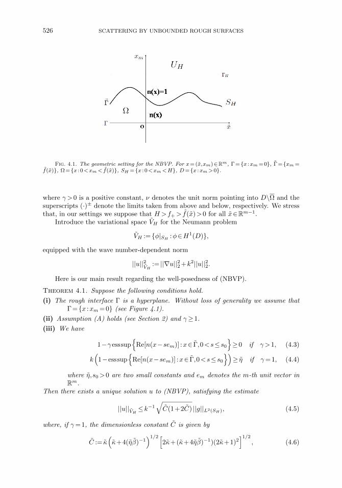
Fig. 4.1. The geometric setting for the NBVP. For x= (x,xm)∈Rm, Γ =x :xm = 0, Γ=xm =f(x), Ω=x : 0<xm<f(x), SH =x : 0<xm<H, D=x :xm>0.

where γ>0 is a positive constant, ν denotes the unit norm pointing into D\Ω and thesuperscripts (·)± denote the limits taken from above and below, respectively. We stressthat, in our settings we suppose that H>f+>f(x)>0 for all x∈Rm−1.

Introduce the variational space VH for the Neumann problem

VH :=φ|SH:φ∈H1(D),

equipped with the wave number-dependent norm

||u||2VH

:= ||∇u||22 +k2||u||22.

Here is our main result regarding the well-posedness of (NBVP).

Theorem 4.1. Suppose the following conditions hold.

(i) The rough interface Γ is a hyperplane. Without loss of generality we assume thatΓ =x :xm= 0 (see Figure 4.1).

(ii) Assumption (A) holds (see Section 2) and γ≥1.

(iii) We have

1−γ esssup

Re[n(x−sem)] :x∈ Γ,0<s≤s0

≥0 if γ>1, (4.3)

k(

1−esssup

Re[n(x−sem)] :x∈ Γ,0<s≤s0

)≥ η if γ= 1, (4.4)

where η,s0>0 are two small constants and em denotes the m-th unit vector inRm.

Then there exists a unique solution u to (NBVP), satisfying the estimate

||u||VH≤k−1

√C(1+2C) ||g||L2(SH), (4.5)

where, if γ= 1, the dimensionless constant C is given by

C := κ(κ+4(ηβ)−1

)1/2[2κ+(κ+4ηβ)−1)(2κ+1)2

]1/2, (4.6)


with

κ=kH, β= δ/√

1+ L2, δ= minx∈Γxm;

and if γ >1, H>1,

C :=

(1+ L2)γ2[(2κ+1)(1+6χ)+2κ]2 +2[γ2κ2(6χ+1)+ κ2]21/2

. (4.7)

with χ := (β(γ−1))−1.

We have several remarks concerning Theorem 4.1.

Remark 4.1.(i) In the case γ= 1, (4.2) reduces to the TE transmission condition. Our condition

(4.4) means that the refractive index has a jump over the interface Γ.

(ii) The condition (ii) covers the TM transmission condition when the refractiveindex is a constant in Ω. Assume n(x) = c0<1 in Ω. In the TM case, it holdsthat γ= 1/c0>1 and the strict equal sign in (4.3) holds.

(iii) The conditions on the refractive index have excluded the case where the en-tire half space xm>0 is occupied by a homogeneous medium. If n(x)≡1 forxm>0, one can readily construct the non-trivial solution u(x) = exp(ikx1) tothe homogeneous Neumann boundary value problem. Hence, the solvability of(NBVP) in this simple case is actually quite involved and it is beyond the scopeof this paper.

To prove Theorem 4.1, we introduce the sesquilinear form b : VH× VH→C by

b(w,v) =(α∇w,∇v

)−k2 (αn(x)w, v)+

∫ΓH

γ−vTγ−wds, (4.8)

with the piecewise constant function α=α(x) given by

α(x) =

1, x∈SH\Ω,γ, x∈Ω.

Then, the sesquilinear form b(·, ·) generates a continuous linear operator B= B(k) : VH→V ∗H such that

(Bw,v) = b(w,v), ∀v∈ VH . (4.9)

If u is a solution to the Neumann problem, then w :=u|SHis a solution of the following

variational problem: find w∈ VH such that

(Bw,v) =−(αg,v) for all v∈ VH . (4.10)

Conversely, by arguing analogously to Lemma 2.3, we see that any solution to thevariational problem (4.10) can be extended to a solution of (NBVP). By (4.9), theadjoint operator B∗ : VH→ V ∗H of B is defined as

(B∗w,v) = (w,Bv) =(Bv,w) = b(v,w), ∀v∈ VH . (4.11)


To verify Theorem 4.1, we may apply Lemma 3.1 following the proof of Theorem3.4. In what follows we prefer to provide another approach by deriving a priori estimatesfor both B and B∗. We first state a basic result from functional analysis. Let X bea Hilbert space, and denote by L(X,X∗) the set of bounded linear operators from Xto its dual space X∗. For A∈L(X,X∗), we denote by A∗ its adjoint operator, whichalso belongs to L(X,X∗). Let KerA and RangeA stand for the kernel and range of A,respectively. Our proof of Theorem 4.1 relies on the following auxiliary lemma.

Lemma 4.2. For any u,v∈X, if there exist some constants C,C∗>0 such that

||u||X ≤C||Au||X∗ , ||v||X ≤C∗||A∗v||X∗ , (4.12)

then the equation Au=f for f ∈X∗ always admits a unique solution u∈X satisfying||u||X ≤C||f ||X∗ .

Proof. It follows from ||u||X ≤C||Au||X∗ that A is injective with a closed rangein X∗, and from ||v||X ≤C∗||A∗v||X∗ that KerA∗=0. Since RangeA= RangeA=(KerA∗)⊥, we obtain RangeA=X∗, i.e., A is also surjective. Here (·)⊥ denotes theset of elements that are orthogonal to (·). This implies the unique solvability of theequation Au=f , f ∈X∗, with the estimate ||u||X ≤C||f ||X∗ .

In order to apply Lemma 4.2, we need to establish the a priori estimates (4.12)with A= B and X= VH . Note that in contrast to Lemma 3.1, it is not necessary tojustify the invertibility of B(k) for small wave numbers, but the a priori estimate for B∗is essentially required in Lemma 4.2.

Theorem 4.1 is a direct consequence of Lemma 4.2 and the following lemma.Lemma 4.3. Suppose that the assumptions in Theorem 4.1 hold.

(i) If w∈ VH is a solution of (4.10), then we have

‖w‖VH≤k−1

√C(1+2C)‖g‖L2(SH),

with C given as in (4.6) and (4.7). Moreover, there holds ||w||VH≤C||Bw||V ∗H

with

C≤ [1+(1+ ||n||L∞(D))]

√C(1+2C)).

(ii) If w∈ VH is a solution of the adjoint equation

(B∗w,v) =−(αg,v) for some g∈L2(SH) and all v∈ VH ,

then w satisfies the same estimates as shown in the first assertion.

Proof. Suppose first that n∈C∞(Ω) and f is a C∞ function with the globalLipschitz constant L>0. Under such regularity assumptions it holds that w∈H2(Ω)and ∇w∈L2(Γ), so that the Rellich identity can be applied.

(i) Let w∈ VH be a solution of (4.10). In view of the derivation of the Rellichidentity (3.16) with f−= 0, we obtain a new Rellich identity in the inhomogeneousdomain Ω:

2k2

∫Ω

xm∂Re(n)

∂xm|w|2dx+2

∫Ω

∣∣ ∂w∂xm

∣∣2dx=−

∫Γ

xm

νm(|∇w−|2−k2Re[n(x)]|w−|2

)−2Re

(∂w−

∂xm

∂w−

∂ν

)ds


+

∫Ω

(|∇w|2−k2Re[n(x)]|w|2

)dx−2Re

∫Ω

xmg∂w−

∂xmdx. (4.13)

Here, ν= (ν1, ·· · ,νm) stands for the unit normal pointing into to D\Ω. Note that inderiving (4.13) we have used the vanishing of the integral term on Γ =x :xm= 0:∫

Γ

xm

∣∣ ∂w∂xm

∣∣2−|∇xw|2 +k2Re[n(x)|w|2ds= 0. (4.14)

On the other hand, since w∈ VH satisfies the equation ∆u+k2u=g in SH \Ω, we obtainanalogously to (4.13) that

2k2

∫SH\Ω

xm∂Re(n)

∂xm|w|2dx+2

∫SH\Ω

∣∣ ∂w∂xm

∣∣2dx=H

∫ΓH

∣∣ ∂w∂xm

∣∣2−|∇xw|2 +k2|w|2ds

+

∫Γ

xm

νm(|∇w+|2−k2|w+|2)−2Re

(∂w+

∂xm

∂w+

∂ν

)ds

+

∫SH\Ω

(∣∣∇w∣∣2−k2|w|2)dx−2Re

∫SH\Ω

xmg∂w+

∂xmdx. (4.15)

Let τ ∈Rm denote the unit tangential direction to Γ such that ∇w=ν∂νw+τ∂τw,and let τm denote the m-th component of τ . Since

∂w

∂xm=em ·∇w=em ·

(ν∂w

∂ν+τ

∂w

∂τ

)=νm

∂w

∂ν+τm

∂w

∂τ,

it holds that

2Re

(∂w

∂xm

∂w

∂ν

)−νm|∇w|2 = 2Re

(νm∣∣∂w∂ν

∣∣2 +τm∂w

∂τ

∂w

∂ν

)−νm

(∣∣∂w∂ν

∣∣2 +∣∣∂w∂τ

∣∣2)=νm

(∣∣∂w∂ν

∣∣2− ∣∣∂w∂τ

∣∣2)+2τmRe

(∂w

∂τ

∂w

∂ν

).

Making use of the transmission conditions (4.2) on Γ, we thus obtain the identity[2Re

(∂w+

∂xm

∂w+

∂ν

)−νm|∇w+|2

]−γ[2Re

(∂w−

∂xm

∂w−

∂ν

)−νm|∇w−|2

]=

[∣∣∂w−∂ν

∣∣2γ(γ−1)+∣∣∂w−∂τ

∣∣2(γ−1)

]νm (4.16)

on Γ. Next, multiplying the first Rellich identity (4.13) by γ and adding the resultingexpression to (4.15) yields∫

Γ

xmνm

[∣∣∂w−∂ν

∣∣2γ(γ−1)+∣∣∂w−∂τ

∣∣2(γ−1)+k2(1−γRe(n))|w|2]ds

+2k2

∫SH

αxm∂Re(n)

∂xm|w|2dx+2

∫SH

α∣∣ ∂w∂xm

∣∣2dx=H

∫ΓH

∣∣ ∂w∂xm

∣∣2−|∇xw|2 +k2|w|2ds


+

∫SH

α(|∇w|2−k2Re[n(x)]|w|2

)dx−2Re

∫SH

αxmg∂w

∂xmdx. (4.17)

Setting v=w in (4.10), we have∫SH

α(x)|∇w|2−k2n(x)|w|2

dx=−

∫ΓH

γ−wTγ−wds−∫SH

αgwdx. (4.18)

Taking the real and imaginary parts of (4.18) and then applying lemmas 2.1 and 2.2, itfollows that (cf. (3.18) and (3.20))∫

SH

α(x)∣∣∇w∣∣2−k2Re[n(x)]|w|2

dx≤−Re

∫SH

αgwdx, (4.19)∫ΓH

| ∂w∂xm

|2−|∇xw|2 +k2|w|2ds≤2kIm

∫SH

αgwdx. (4.20)

Set Λ−= min1,γ, Λ+ = max1,γ. Inserting the estimates (4.19), (4.20) into (4.17)and using the monotonicity of Re(n(x)) and the Cauchy-Schwarz equality, we can esti-mate the first term on the left hand side of (4.17) by∫

Γ

xmνm

[∣∣∂w−∂ν

∣∣2γ(γ−1)+∣∣∂w−∂τ

∣∣2(γ−1)+k2(1−γRe(n))|w|2]ds+2Λ−

∣∣∣∣ ∂u∂xm

∣∣∣∣22

≤2kHIm

∫SH

αgwdx−Re

∫SH

αgwdx−2Re

∫SH

αxmg∂w

∂xmdx

≤ (2kH+1)Λ+‖g‖2‖w‖2 +2Λ+H∣∣∣∣ ∂w∂xm

∣∣∣∣2||g||2. (4.21)

This, together with the Young’s inequality ab≤ εa2 +b2/(4ε) for any a,b,ε>0, impliesthe estimate for the L2-norm of ∂u/∂xm over SH :

|| ∂w∂xm

||22≤ (2kH+1)Λ‖g‖2‖w‖2 +Λ2H2||g||22, Λ := Λ+/Λ−. (4.22)

We proceed with the proof by studying the cases γ= 1 and γ>1 separately.

Case (a): Suppose the condition (4.4) holds for γ= 1.In this case it holds that Λ+ = Λ−= Λ = 1. In view of condition (iii) of Theorem 4.1

and the inequalities (4.21) and (4.22), again applying Young’s inequality gives

β kη ||w||2L2(Γ)

≤ (2kH+1)‖g‖2‖w‖2 + || ∂w∂xm

||22 +H2 ||g||22

≤2(2kH+1)‖g‖2‖w‖2 +2H2 ||g||22, (4.23)

with β := δ/√

1+ L2. Therefore, combining (4.22) and (4.23), we obtain (see [24] forthe first inequality)

||w||22≤2H ||w||2L2(Γ)

+H2 || ∂w∂xm

||22

≤H(2kH+1)(H+4(kηβ)−1) ||g||2 ||w||2 +H3(H+4(kηβ)−1) ||g||22. (4.24)

Hence, using Young’s inequality,

||w||2≤C0 ||g||2


with C0 =H(H+4(kηβ)−1)1/2[2H+(H+4(kηβ)−1)(2kH+1)2

]1/2. From (4.19), we

obtain the estimate

||∇w||22≤||g||2 ||w||2 +k2 ||w||22≤C0 (1+k2C0)||g||22,

and thus

||w||2VH

=k2||w||22 + ||∇w||22≤C0 (1+2k2C0)||g||22≤k−2C (1+2C)||g||22, (4.25)

where the constant C=k2C0 can be reformulated as in (4.6). Arguing analogously to[8, Lemma 4.5], we obtain

||w||VH≤C||Bw||V ∗H , C≤1+(1+ ||n||L∞(D))

√C(1+2C). (4.26)

Case (b): Suppose the condition (4.3) holds when γ>1.We have Λ+ = Λ =γ, Λ−= 1. Since νm≥ (1+ L2)−1/2 on Γ, it follows from (4.21)

and (4.22) that

β(γ−1)||∇w||2L2(Γ)

≤2(2kH+1)γ‖g‖2‖w‖2 +2γ2H2||g||22. (4.27)

In order to estimate ||u||L2(Γ), we have to use another Rellich identify over the strip

SH\Ω. Multiplying ∂w/∂xm to both sides of the equation

∆w+k2w=g in SH\Ω

and then integrating by parts yields

2Re

∫SH\Ω

g∂w

∂xmdx= 2Re

∫SH\Ω

∂w

∂xm(∆w+k2w)dx

=

(∫ΓH

−∫

Γ

)−νm|∇w|2 +νmk

2|w|2 +2Re

(∂w+

∂xm

∂w+

∂ν

)ds

Rearranging the terms in the above expression and making use of (4.19), (4.20),∫Γ

−νm|∇w|2 +νmk

2|w|2 +2Re

(∂w+

∂xm

∂w+

∂ν

)ds

≤2kIm

∫SH

αgwdx−2Re

∫SH\Ω

g∂w

∂xmdx

≤2kγ ||g||2 ||w||2 +2||g||2 ||∂w/∂xm||2. (4.28)

Combining (4.22), (4.28), and (4.27), we obtain an upper bound of ||w||L2(Γ):

k2√1+ L2

||w||2L2(Γ)

≤3||∇w||2L2(Γ)

+γ (2kH+2k+2) ||g||2||w||2 +(γ2H2 +1)||g||22

≤γ[(2kH+1)(1+6χ)+2k]||g||2||w||2 +[γ2H2(6χ+1)+1] ||g||22

with χ := (β(γ−1))−1. Now, applying the first inequality in (4.24) we find after somesimple calculations that ||w||2≤C0||g||2 with

C0 =k−4(1+ L2)γ2[(2kH+1)(1+6χ)+2k]2 +2k−2[γ2H2(6χ+1)+1]2

1/2

.


Finally, arguing analogously to (4.25) and (4.26), we can get the estimate (4.5) withthe coefficient C=k2C0 given as in (4.7). Note that in the last step we have used thefact that κ=kH >k if H>1. If H≤1, the constant C depends on both κ and k. Thisfinishes the proof of the first assertion when n∈C∞(Ω) and f ∈C∞(R).

Having established the a priori estimate for C∞-interfaces, we now adapt Necas’method [27, Chap. 5] of approximating a Lipschitz graph by smooth surfaces to justifythe a priori estimate (4.5) when f is a Lipschitz continuous function and n∈C∞(Ω).Similar arguments are employed in [20] for the Helmholtz equation in the periodic caseand in [17, 18] for the Navier equation in linear elasticity.

Choose C∞-smooth functions fj such that (see e.g., [29, Lemma 3.10])

Γj :=x :xm= fj(x),x∈Rm−1⊂Ω, j∈N,sup|fj(x)− f(x)| : x∈Rm−1→0, as j→∞,|fj(x1)− fj(x2)|≤ L|x1− x2|, for all x1,x2∈Rm−1 and j∈N,

where L>0 is the Lipschitz constant of f (cf. (4.1)). Accordingly, introduce the domainΩj and the piecewise constant function αj(x) in the same way as Ω and α with the

interface Γ replaced by Γj . Define the sesquilinear form bj(·, ·) as the same as b (see(4.8)) with α replaced by αj . Repeating the previous proof for smooth interfaces, we

can get a solution wj ∈ VH to the variational equation bj(w,v) =−(αj g,v) for all v∈ VH ,with the estimate

||wj ||VH≤k−1

√Cj(1+2Cj) ||g||2 for allj∈N.

Moreover, we have Cj→ C as j→∞, where C is given as in Theorem 4.1. Hence, thereexists a weakly convergent sequence, which we still denote by wj , satisfying wjw

in VH for some w∈ VH . We claim that w is just the solution to the original varia-tional formulation b(w,v) =−(αg,v) for all v∈ VH . To see this, we need to prove theconvergence

bj(wj ,v)→ b(w,v), (αj g,v)→ (αg,v) as j→+∞,

for any v∈ VH . This is obvious in the case γ= 1 where it holds that αj =α= 1. Below

we suppose that γ 6= 1. Since wjw in VH , we have∫ΓH

γ−vTγ−wjds→∫

ΓH

γ−vTγ−wds as j→+∞.

Next we shall prove that (αj∇wj ,∇v)→ (α∇w,∇v), as j→+∞. Obviously,

(αj∇wj ,∇v)−(α∇w,∇v) = ((αj−α)∇w,∇v)+(αj(∇wj−∇w),∇v).

We have the convergence (αj(∇wj−∇w),∇v)→0 as j→+∞, since wjw in VH and||αj ||L∞(SH)≤maxγ,1. To prove the convergence of the first term on the right hand

side of the previous equation, we define the domain Kj := Ω\Ωj in which αj =γ, butα= 1. Then we have∫

SH

(αj−α)∇w ·∇vdx= (γ−1)

(∫Kj∩|x|≤M

+

∫Kj∩|x|>M

)∇w ·∇vdx


for any M>0. Since w,v∈ VH , we can choose M sufficiently large so that the integralover Kj ∩|x|>M can be arbitrarily small for any j∈N. As j→∞, the integral overKj ∩|x|<M tends to zero, due to the fact that the volume of Kj ∩|x|<M tendsto zero. Hence, ((αj−α)∇w,∇v)→0 as j→+∞. To sum up, we get (αj∇wj ,∇v)→(α∇w,∇v), and similarly, (αjnwj ,v)→ (αnw,v), (αjg,v)→ (αg,v). As a consequence,

we obtain wjw in VH , and thus

||w||VH≤ limsup

j→+∞||wj ||VH

≤k−1||g||2 limsupj→+∞

√Cj(1+2Cj)≤k−1

√C(1+2C)||g||2.

This finishes the proof if the interface Γ is a graph of a Lipschitz continuous functionand n∈C∞(Ω). The case n∈L∞(Ω) can be treated as before in the proof of Lemma3.5 (see also [29]). The first assertion of Lemma 4.3 is thus proven.

(ii) Assume w∈ VH is a solution of the adjoint equation

(B∗w,v) = b(v,w) =−(αg,v), for allv∈ VH . (4.29)

From the definition of the sesquilinear form b (see (4.8)), we derive that

b(v,w) = (α∇w,∇v)−k2(αn(x)w,v)+

∫ΓH

γ−vT∗γ−wds, (4.30)

where T ∗ is the adjoint of the DtN map T . In view of the proof of the first assertion,only the monotonicity of the real part of the refractive index n(x) (assumption A) andthe positivity of the real part of the DtN map (Lemma 2.1 (ii)) were involved, but nottheir imaginary parts, for instance, in the proof of (4.23) and (4.20). Therefore, theprevious proof carries over to the solution of (4.29) with the same a priori estimate.The proof of Lemma 4.3 is complete.

5. Solvability for incident plane and point source wavesIn this section we shall consider incident plane and point source waves, relying on

the well-posedness results for inhomogeneous terms and following the argument of [5].We first restrict ourselves to two-dimensional incident plane waves and then discuss theresults for point source waves in Rm (m= 2,3).

Suppose a two-dimensional incident plane wave of the form

uin= exp(ikx ·d), d= (cosθ,sinθ), θ∈ (−π/2,0), (5.1)

is incident onto the rough surface Γ⊂R2 from above. We shall adapt the weightedSobolev spaces used in [5] for sound-soft rough surfaces to our generalized impedanceand Neumann boundary value problems in R2. For %∈R and H≥f+, denote by H1

%(SH)the weighted Sobolev space defined as

‖u‖H1%(SH) =

[∫SH

(∣∣(1+ |x1|2)%/2u∣∣2 +

∣∣∣∇[(1+ |x1|2)%/2u]∣∣∣2)dx]1/2

.

Obviously, the restriction of the plane wave (5.1) to SH (H>f+) belongs to the spaceH1%(SH) for all %<−1/2. One can also employ the following equivalent norm to || · ||VH,%

:

||u||′ :=[∫

SH

(1+ |x1|2)%(∣∣u∣∣2 +

∣∣∇u|2)dx]1/2

, u∈VH,%.


Moreover, we introduce

Hs%(ΓH) := (1+x2

1)−%/2Hs(ΓH), %∈R,

with the norm

||u||Hs%(ΓH) := ||(1+x2

1)%/2u(x1)||Hs(ΓH).

Our scattering problem will be posed over the weighted Hilbert space

(GIBVP): VH,% :=φ|SH:φ∈H1

%(D),φ∈H1%(Γ),

(NBVP): VH,% :=φ|SH:φ∈H1

%(D),

corresponding to the generalized impedance and Neumann boundary value problems,equipped with the weighted norm

‖|u‖|VH,%:=‖u‖H1

%(SH) +‖u‖H1%(Γ), ‖|u‖|VH,%

:=‖u‖H1%(SH),

respectively. The space H1%(Γ) will be equipped with the norm

‖u‖H1%(Γ) =

[∫Γ

(1+ |x1|2)%(|u|2 + |∇Γu|2)dx

]1/2

,

where the symbol ∇Γ denotes again the surface gradient. Since Γ is the graph of thefunction f(x1), the above norm ‖u‖H1

%(Γ) is equivalent to

||u||H1%(Γ) := ||(1+ |x1|2)%/2uf(x1)||H1(R).

If %= 0, we have the coincidence VH,0 =VH , VH,0 = VH , where VH ,VH are the non-weighed Sobolev spaces used in Sections 3 and 4, respectively. Below we collect someproperties of Hs

%(·), which will be used for our subsequent analysis.

Proposition 5.1.(i) The Fourier transform F is an isomorphism of Hs

%(R) onto H%s (R) for all s,%∈R.

(ii) The trace operators

γ− :H1%(SH)→H1/2

% (ΓH) , γ+ :H1%(Uh\UH)→H1/2

% (ΓH), H >h,

are continuous.

(iii) The dual space of Hs%(R) with respect to the L2 scalar product is H−s−%(R), that is,

Hs%(R)∗=H−s−%(R) for all s,%∈R.

With these properties for Fourier transforms, it has been shown in [5, Lemma 3.3]that the upward Angular Spectrum Representation (2.6) can be interpreted as a linear

functional from H1/2% (ΓH) to H1

%(Sa) for any a>H if and only if %>−1. Moreover, the

DtN map defined as in (2.11) is a bounded linear map from H1/2% (ΓH) to H

−1/2% (ΓH)

for any |%|<1. Before formulating the variational formulations for plane waves, westill need to interpret the differential operator divΓ(µ∇Γ·) in weighted Sobolev spaces.For v∈H1

%(∂D), the surface gradient ∇Γv lies in the tangential space L2t,%(Γ) :=V ∈

L2%(∂D) :ν ·V = 0. The operator divΓ(µ∇Γu) is then defined in the space H%

−1(Γ) =(H1−%(Γ))∗ by ⟨

divΓ(µ∇Γu),v⟩%

=−∫

Γ

µ∇Γu ·∇Γvds, ∀v∈H1−%(Γ), (5.2)


where⟨·,·⟩%

stands for the duality pairing in⟨H%−1(Γ),H1

−%(Γ)⟩

extending the inner

product in L2(Γ), and the right hand side of (5.2) is the dual between H0−%(Γ) and

H%0 (Γ). Now we formulate the variational formulations for Neumann and generalized

impedance boundary value problems with an incident plane wave in the following way:for −1<ρ<−1/2,

(GIBVP): find u∈VH,% such that b(u,v) =

∫ΓH

ψvds, ∀v∈VH,−%, (5.3)

(NBVP): find u∈ VH,% such that b(u,v) =

∫ΓH

ψvds, ∀v∈ VH,−%, (5.4)

where b :VH,%×VH,−%→C, b : VH,%× VH,−%→C, defined as in (2.17) and (4.8) respec-tively, are both bounded sesquilinear forms, and

ψ :=∂uin

∂x2|ΓH−T (uin|ΓH

)∈H−1/2% (R).

Note that the right hand sides of the above variational formulations lead to bounded

linear functionals over VH,−% resp. VH,−% due to the dual⟨H−1/2% (R),H

1/2−% (R)

⟩. More-

over, using the relation F exp(ikx1 cosθ) = δ(ξ−kcosθ) (the δ-function concentrated atξ=kcosθ) and the definition of T (see (2.11)), we see

T (uin|ΓH) =

∫R

exp(iξx1)z(ξ;k)δ(ξ−kcosθ)dξ exp(ikH sinθ)

=−iksinθexp(ik(x1 cosθ+H sinθ)),

and thus

ψ=−i2ksinθexp(ik(x1 cosθ+H sinθ)).

The uniqueness and existence of solutions of (5.3) and (5.4) follow immediately fromthe solvability results in the non-weighted setting %= 0 and the perturbation argumentused in the proof of [5, Theorem 4.1] that relies essentially on a parameter-dependentcommutator estimate for the DtN map in weighted spaces. A significant idea of [5] isto reduce the invertibility of the operator corresponding to the left hand side of (5.3)resp. (5.4) for % 6= 0 to that for %= 0. To achieve this, the authors there introduced areal parameter into the commutator estimate of the convolution operator (associatedwith the DtN map) with a non-smooth square-root symbol. Since the DtN map in ourstudies is exactly the same as that considered in [5], this approach extends directly to ourboundary value problems with only minor changes. We summarize the well-posednessfor incident plane waves as follows:

Theorem 5.2. Under the conditions in Theorem 3.4 (resp. Theorem 4.1), the vari-ational problem (5.3) (resp. (5.4)) has exactly one solution in the space VH,% (resp.

VH,%) for every H>f+ and −1<%<−1/2. Hence, the Neumann (resp. generalizedimpedance) boundary value problem with an incident plane wave is unique solvable inthe space mentioned above.

To the best of the authors’ knowledge, it is still unknown how to establish thevariational approach for three-dimensional incident plane waves. Difficulties arise fromthe fact that, as explained in [5], the radiation condition (2.6) can be interpreted as alinear functional on H1

%(ΓH) only if %>−1 but the restriction of a three-dimensional


plane wave to the strip SH lies in the space H1%(SH) for any %<−1. However, this

dilemma can be avoided in the case of an incident point source wave. Define an acousticpoint source wave Gin(x;y) by

Gin(x;y) =

i

4H

(1)0 (k|x−y|), m= 2,

eik|x−y|

4π|x−y|, m= 3,

x= (x,xm),y= (y,ym)∈Rm, x 6=y,

where H(1)0 (·) denotes the first kind Hankel function of order zero. In R2, the asymptotic

behavior of the Hankel function for large arguments implies that Gin(x;y),∇xGin(x;y)∼O(|x|−1/2) as |x|→∞. Hence, it holds that Gin(x;y)∈H1

%(SH) for any %<0 and ym>H, which is also true in R3. As a consequence of Theorem 5.2 we get

Theorem 5.3. Let the conditions in Theorem 3.4 (resp. Theorem 4.1) hold and letuin(x) =Gin(x,y) be an incident point source wave with ym>f+. Then the rough surfacescattering problem with GIBC (resp. NBC) has exactly one solution u−uin in theweighted Sobolev space VH,% (resp. VH,%) for every H>f+ and −1<%<0.

Acknowledgement. This work was finished when G. Hu visited AMSS of theChinese Academy of Sciences, Beijing in 2013. The hospitality of AMSS and the supportfrom German Research Association (DFG: HU2111) and WIAS, Berlin are gratefullyacknowledged. G. Hu would also like to thank H. Haddar for stimulating discussions onGIBC and J. Elschner for the constant encouragement at WIAS. The research of X. Liuand B. Zhang was supported in part by the NNSF of China 11101412 and 61379093,and the work of F. Qu was partially supported by the NNSF of China 11201402 andAMSS of the Chinese Academy of Sciences, Beijing. The authors thank the referees fortheir constructive comments and suggestions which helped improve the paper.

REFERENCES

[1] T. Arens and T. Hohage, On radiation conditions for rough surface scattering problems, IMA J.Appl. Math., 70, 839–847, 2005.

[2] F.X. Becot, P.J. Thorsson, and W. Kropp, An efficient application of equivalent sources to noisepropagation over inhomogeneous ground, Acta Acoust. United Ac., 88, 853–860, 2002.

[3] P. Boulanger, K. Attenborough, S. Taherzadeh, T. WatersFuller, and K.M. Li, Ground effect overhard rough surfaces, J. Acoust. Soc. Am., 104, 1474–1482, 1998.

[4] A.S. Bonnet-Bendhia and F. Starling, Guided waves by electromagnetic gratings and non-uniqueness examples for the diffraction problem, Math. Meth. Appl. Sci., 17, 305–338, 1994.

[5] S.N. Chandler-Wilde and J. Elschner, Variational approach in weighted Sobolev spaces to scat-tering by unbounded rough surfaces, SIAM J. Math. Anal., 42, 2554–2580, 2010.

[6] S.N. Chandler-Wilde, E. Heinemeyer, and R. Potthast, Acoustic scattering by mildly rough un-bounded surfaces in three dimensions, SIAM J. Appl. Math., 66, 1002–1026, 2006.

[7] S.N. Chandler-Wilde, E. Heinemeyer, and R. Potthast, A well-posed integral equation formulationfor three-dimensional rough surface scattering, Proc. Roy. Soc. London A462, 3683–3705,2006.

[8] S.N. Chandler-Wilde and P. Monk, Existence, uniqueness, and variational methods for scatteringby unbounded rough surfaces, SIAM J. Math. Anal., 37, 598–618, 2005.

[9] S.N. Chandler-Wilde, P. Monk, and M. Thomas, The mathematics of scattering by unbounded,rough, inhomogeneous layers, J. Comput. Appl. Math., 204, 549–559, 2007.

[10] S.N. Chandler-Wilde and C.R. Ross, Scattering by rough surfaces: the Dirichlet problem for theHelmholtz equation in a non-locally perturbed half-plane, Math. Meth. Appl. Sci., 19, 959–976,1996.

[11] S.N. Chandler-Wilde and B. Zhang, A uniqueness result for scattering by infinite rough surfaces,SIAM J. Appl. Math., 58, 1774–1790, 1998.


[12] S.N. Chandler-Wilde and B. Zhang, Electromagnetic scattering by an inhomogeneous conductingor dielectric layer on a perfectly conducting plate, Proc. Roy. Soc. London A454, 519–542,1998.

[13] S.N. Chandler-Wilde and B. Zhang, Scattering of electromagnetic waves by rough interfaces andinhomogeneous layers, SIAM J. Math. Anal., 30, 559–583, 1999.

[14] M. Duran, I. Muga, and J.C. Nedelec, The Helmholtz equation in a locally perturbed half-spacewith passive boundary, IMA J. Appl. Math., 71, 853–876, 2006.

[15] M. Duran, I. Muga, and J.C. Nedelec, The Helmholtz equation in a locally perturbed half-spacewith non-absorbing boundary, Arch. Rat. Mech. Anal., 191, 143–172, 2009.

[16] M. Durufle, H. Haddar, and P. Joly, Higher order generalized impedance boundary conditions inelectromagnetic scattering problems, C.R. Physique, 7, 533–542, 2006.

[17] J. Elschner and G. Hu, Scattering of plane elastic waves by three-dimensional diffraction gratings,Math. Models Meth. Appl. Sci., 22, 1150019, 2012.

[18] J. Elschner and G. Hu, Elastic scattering by unbounded rough surfaces, SIAM J. Math. Anal., 44,4101–4127, 2012.

[19] J. Elschner and G. Hu, Elastic scattering by unbounded rough surfaces: solvability in weightedSobolev spaces, Appl. Anal., doi:10.1080/00036811.2014.887695, 2014.

[20] J. Elschner and M. Yamamoto, An inverse problem in periodic diffractive optics: reconstructionof Lipschitz grating profiles, Appl. Anal., 81, 1307–1328, 2002.

[21] H. Haddar and A. Lechleiter, Electromagnetic wave scattering from rough penetrable layers, SIAMJ. Math. Anal., 43, 2418–2443, 2011.

[22] H. Haddar and A. Lechleiter, Asymptotic models for scattering from unbounded media with highconductivity, Math. Model. Numer. Anal., 44, 1295–1317, 2010.

[23] H. Haddar, P. Joly, and H.-M. Nguyen, Generalized impedance boundary conditions for scatteringby strongly absorbing obstacles: the scalar case, Math. Models Meth. Appl. Sci., 15, 1273–1300, 2005.

[24] A. Lechleiter and S. Ritterbusch, A variational method for wave scattering from penetrable roughlayers, IMA J. Appl. Math., 75, 366–391, 2010.

[25] P. Li, H. Wu, and W. Zheng, Electromagnetic scattering by unbounded rough surfaces, SIAM J.Math. Anal., 43, 1205–1231, 2011.

[26] P. Li and J. Shen, Analysis of the scattering by an unbounded rough surface, Math. Meth. Appl.Sci., 35, 2166–2184, 2012.

[27] J. Necas, Les Methodes Directes en Theorie des Equations Elliptiques, Masson, Paris, 1967.[28] J.A. De Santo, Scattering by rough surfaces, in Scattering: Scattering and Inverse Scattering in

Pure and Applied Sciences, R. Pike and P. Sabatier (eds.), Academic Press, New York, 15–36,2002.

[29] M. Thomas, Analysis of Rough Surface Scattering Problems, PhD thesis, University of Reading,2006.

[30] A.G. Voronovich, Wave Scattering from Rough Surfaces, Second Edition, Springer, Berlin, 1998.[31] B. Zhang and S.N. Chandler-Wilde, Acoustic scattering by an inhomogeneous layer on a rigid

plate, SIAM J. Appl. Math., 58, 1931–1950, 1998.[32] B. Zhang and S.N. Chandler-Wilde, Integral equation methods for scattering by infinite rough

surfaces, Math. Meth. Appl. Sci., 26, 463–488, 2003.

Documents

VARIATIONAL APPROACH TO SCATTERING BY UNBOUNDED ROUGH ...€¦ · VARIATIONAL APPROACH TO SCATTERING BY UNBOUNDED ROUGH SURFACES WITH NEUMANN AND GENERALIZED IMPEDANCE BOUNDARY