Investigation of Limit Cycle Oscillations Using Aeroelastic-HarmonicBalance Method

Marques, S., Yao, W., & Hayes, R. (2014). Investigation of Limit Cycle Oscillations Using Aeroelastic-HarmonicBalance Method. Paper presented at 4th EASN Workshop on Flight Physics and Aircraft Design, Aachen,Germany.

Document Version:Peer reviewed version

Queen's University Belfast - Research Portal:Link to publication record in Queen's University Belfast Research Portal

Publisher rightsCopyright - Simao Marques, Weigang Yao, Richard Hayes, all rights reserved.

General rightsCopyright for the publications made accessible via the Queen's University Belfast Research Portal is retained by the author(s) and / or othercopyright owners and it is a condition of accessing these publications that users recognise and abide by the legal requirements associatedwith these rights.

Take down policyThe Research Portal is Queen's institutional repository that provides access to Queen's research output. Every effort has been made toensure that content in the Research Portal does not infringe any person's rights, or applicable UK laws. If you discover content in theResearch Portal that you believe breaches copyright or violates any law, please contact openaccess@qub.ac.uk.

Download date:06. Jul. 2018

Investigation of Limit Cycle Oscillations Using

Aeroelastic-Harmonic Balance Method

Simao Marques, ∗Weigang Yao† and Richard Hayes†‡

Queen’s University Belfast, Belfast, BT9 5AH, Northern Ireland

This work investigates limit cycle oscillations in the transonic regime. A novel approachto predict Limit Cycle Oscillations using high fidelity analysis is exploited to acceleratecalculations. The method used is an Aeroeasltic Harmonic Balance approach, which hasbeen proven to be efficient and able to predict periodic phenomena. The behaviour of limitcycle oscillations is analysed using uncertainty quantification tools based on polynomialchaos expansions. To improve the efficiency of the sampling process for the polynomial-chaos expansions an adaptive sampling procedure is used. These methods are exercisedusing two problems: a pitch/plunge aerofoil and a delta-wing. Results indicate that Machn. variability is determinant to the amplitude of the LCO for the 2D test case, whereas forthe wing case analysed here, variability in the Mach n. has an almost negligible influencein amplitude variation and the LCO frequency variability has an almost linear relationwith Mach number. Further test cases are required to understand the generality of theseresults.

Nomenclature

Latin Symbols

A Harmonic Balance frequency domain matrixb, c aerofoil semi-chord and chord, respectivelyCFL Courant-Friedrichs-LewyD Harmonic Balance operator matrixE energyE Transformation matrix between frequency and time domainsf fluid force acting on structureF,G,Hconvective fluxes for fluid equationsh plunge coordinateI HB residualK structure stiffness matrixL frequency updating figure of meritM structure mass matrixp pressureR vector of fluid and/or structural equation residualt time stepU∞ free-stream velocityu, v, wfluid cartesian velocity componentsV, Vs reduced velocity and velocity indexW vector of fluid unknownsx,y vector of structural unknownsGreek Symbols

α angle of attack

∗Lecturer, School of Mechanical & Aerospace Engineering, QUB, Belfast. s.marques@qub.ac.uk†Research Fellow, School of Mechanical & Aerospace Engineering, QUB, Belfast. w.yao@qub.ac.uk‡PhD Student, School of Mechanical & Aerospace Engineering, QUB, Belfast. rhayes04@qub.ac.uk - Copyright c© Simao

Marques and Weigang Yao and Richard Hayes. All rights reserved.

1 of 8

ω, κ frequency and reduced frequency, κ = 2ωU∞c

ρ densityτ pseudo-time step

I. Introduction

Industry standard practices to solve aeroelastic problems rely heavily upon linear aerodynamic theory.This has well known limitations in the transonic regime and where other sources of aerodynamic non-linearities are present (e.g., unsteady viscous flows), hence a clear need for physics based modelling tools hasemerged as identified by Noll et al.

1 When nonlinearities are present, aeroelastic instabilities can lead tooscillations that become limited and limit cycle oscillations are observed. This is a problem of considerablepractical interest and is well documented for in-service aircraft.2,3 The presence of nonlinearities, eitherstructural or aerodynamic, poses additional challenges both in terms of complexity and computational re-sources, by requiring higher-fidelity analysis. Hence, several efforts have been made to address both issuesof retaining the required level of fidelity to capture the relevant physics, while at the same time limiting thecomputational resources required for such analysis.

Advances in CFD (Computational Fluid Dynamics) methods allowed the coupling of nonlinear aerody-namic models with CSD (Computational Structural Dynamics) in the time domain; however this type ofanalysis is used as a last resort tool due to the high computational cost. To circumvent the need for expen-sive simulations, several kinds of Reduced Order Models (ROM) have been proposed and used, for example:Proper Orthogonal Decomposition (POD),4,5 Volterra Series,6–8 Neural Networks.9

An alternative to ROM and full time domain analysis of aeroelastic oscillatory problems is to employthe non-linear Harmonic Balance (HB) method. New Harmonic Balance methods have been developedfor CFD time periodic flows;10,11 in such methods, the periodicity of the flow is exploited and representtime dependent flow variables as Fourier series and recast the problem in terms of Fourier coefficients.These methods have been successful in predicting unsteady flows efficiently in diverse applications: forcedmotions,12,13 helicopter rotors,14 turbomachinery.10,15,16 Thomas et al.extended the HB formulation topredict Limit Cycle Oscillations for fixed wing aircraft.3 Ekici and Hall further reduced the computationalcost of predicting LCOs with HB methods, by proposing a one-shot method to analyze 1-DOF LCO inturbomachinery flows.15 Recently the authors extended this approach for fixed wing LCO computations.17

In this paper, this last variation of the HB method for LCO predictions is formulated around an implicitmethod originally proposed in ref.,12 yielding a faster, more robust approached to nonlinear aeroelasticproblems such as LCOs.

II. Flow Solver

The semi-discrete form of an arbitrary system of conservation laws such as the three-dimensional Eulerequations can be described as:

∂W

∂t= −R(W) (1)

where R is the residual error of the steady-state solution:

R =∂F

∂x+

∂G

∂y+

∂H

∂z(2)

Here W is the vector containing the flow variables and F, G, H are the fluxes, which are given by:

W =

ρ

ρu

ρv

ρw

ρE

, F =

ρu

ρuu+ p

ρuv

ρuw

u(ρE + p)

, G

ρv

ρuv

ρvv + p

ρvw

v(ρE + p)

, H =

ρw

ρuw

ρvw

ρww + p

w(ρE + p)

, (3)

2 of 8

The steady state solution of the Euler equations is obtained by marching the solution forward in time bysolving the following discrete nonlinear system of equations:

Wn+1 −Wn

∆t= −Rn (4)

To discretize the residual convective terms a Roe flux function18 together with MUSCL interpolation isused,19 the Van Albada limiter is used to obtain 2nd order accuracy.

III. Harmonic Balance Formulation

As discussed in the introduction, several authors have demonstrated the suitability of HB methods as analternative to time marching CFD formulations for periodic flow problems. To obtain the HB version of theflow solver, we follow the methodology proposed by Woodgate12 for implicit Harmonic Balance methods,which is summarised next. Consider the semidiscrete form as a system of ordinary differential equations

I(t) =dW(t)

dt+R(t) = 0 (5)

The solution of W and R in eq.(5) can be approximated to be a truncated Fourier series of NH harmonicswith a fundamental frequency ω:

W(t) ≈ W0 +

NH∑

n=1

(W2n−1 cos(nωt) + W2n sin(nωt)) (6)

R(t) ≈ R0 +

NH∑

n=1

(R2n−1 cos(nωt) + R2n sin(nωt)) (7)

Hence, eq.(5) can also be approximated by a truncated Fourier series,

I(t) ≈ I0 +

NH∑

n=1

(I2n−1 cos(nωt) + I2n sin(nωt)) (8)

which results in the following system of equations

I0 = R0 (9)

I2n−1 = ωnW2n + R2n−1 (10)

I2n = −ωnW2n−1 + R2n (11)

which results in a system of (2NH +1) equations for the Fourier coefficients that can be expressed in matrixform as

ωAW + R = 0 (12)

where A is given by:

A =

0

J1

. . .

JNH

(2NH+1)×(2NH+1)

, Jn = n

[

0 1

−1 0

]

, n = 1, 2, . . . , NH (13)

To overcome the difficulties in expressing the Fourier coefficient in R as functions of W, Hall et al.10 proposedto cast the system of equations back in the time domain, where the flow variables and residual solutions aresplit into (2NH + 1), discrete, equally spaced intervals over the period T = 2π

ω.

Whb =

W(t0 +∆t)

W(t0 + 2∆t)...

W(t0 + T )

, Rhb =

R(t0 +∆t)

R(t0 + 2∆t)...

R(t0 + T )

, (14)

3 of 8

It is possible to define a transformation matrix, E that relates the frequency domain variables to their HBtime domain counterpart10

W = EWhb R = ERhb (15)

Substituting the terms in eq.(15) in eq.(12), it becomes:

ωAW + R = 0 = ωAEWhb +ERhb = ωE−1AEWhb +Rhb =

= ωDWhb +Rhb = 0 (16)

where D = E−1AE, the elements in matrix D are given by:

Di,j =2

2NH + 1

NH∑

k=1

k sin

(

2πk(j − i)

2NH + 1

)

(17)

To solve eq.(16) a pseudo time step of the form is introduced:

dWhb

dτ+ ωDWhb +Rhb = 0 (18)

To solve eq.(18), any steady-state CFD time marching method can be used. In this work, a 4th − orderRunge-Kutta method is used.

IV. Aeroelastic Formulation

Consider a generic dynamic system without damping, whose behaviour can be described using the equa-tions of motion given by:

Mx+Kx = f (19)

where M, K, respectively, represent the mass and stiffness of the system and f is an external force (inthis work, this will be the aerodynamic force, f = f(w, ω,x) ). This equation can be transformed into astate-space form, giving:

y = Asy +Bsf (20)

where:

As =

[

0 I

−M−1K 0

]

, Bs =

[

0

M−1

]

, y =

[

x

x

]

(21)

Equation (20) has a similar form to the flow equations, hence it can be solved using the Harmonic Balancemethod described in the previous section, resulting in the following HB format of eq.(20):

ωDyhb = Asyhb +Bsfhb (22)

where D is the same HB operator described in eq.(17). Equation (22) can be solved using the same pseudotime technique previously presented, leading to the following system of equations:15

dyhb

dτ+ ωDyhb− (Asyhb +Bsfhb) = 0 (23)

Equation (18) together with eq.(23) represent the nonlinear coupled aeroelastic system; when solving theaeroelastic system of equations, at each iteration, the generalized aerodynamic forces are computed usingeq.(18), which will feed into eq.(23). The solution from eq.(23) will provide new generalized displacementand velocities to eq.(18). The CFD grid is deformed using Transfinite Interpolation and the mesh velocitiesare approximated by finite-differences9.

4 of 8

IV.A. Prediction of Limit-Cycle Oscillations

The prediction of LCO depends on determining a solution vector for [ω,y] (the subscript hb is dropped forsimplicity), that satisfies both the structural governing equation eq.(23) and eq.(18). If the LCO frequency,ω, is given beforehand, then the coupling itself becomes a fixed point iteration process which is extensivelyused for static aeroelastic problems in its time domain counterpart.13 Inspired by the results of Blanc et al.,13

the Yao and Marques17 proposed to transform this LCO prediction problem into a fixed point algorithm withfrequency updating. To determine the LCO condition using eq.23, the frequency updating can be achievedby minimizing the L2 norm of the residual R of eq.(23).15 First, define a figure of merit, in this case:

Ln =1

2RTR =

1

2[ωDy − (Asy +Bsf)]

T[ωDy − (Asy +Bsf)] (24)

The frequency is updated by minimizing the residual R but, critically, without freezing the aerodynamicforces f , leading to:

∂Ln

∂ω=

(

Dy −Bs

∂f

∂ω

)T

[ωDy − (Asy +Bsf)] (25)

If the frequency ω is not at the LCO condition, the residual R for the displacement is not able to converge.Therefore, the idea is to update the frequency at every ni iterations. The full details of the algorithm aregiven in.17 When compared to the standard fixed point algorithm described by Blanc et al.,13 the newalgorithm introduces some extra computational effort to compute the gradient of the aerodynamic forcewith respect to the frequency. However, the frequency is only updated every ni iterations ( enough to reducethe residual by three orders of magnitude and allow an accurate estimation of eq.(25), typically every 10-15iterations) and the perturbation is sufficiently small, minimizing the computational cost.

V. Results

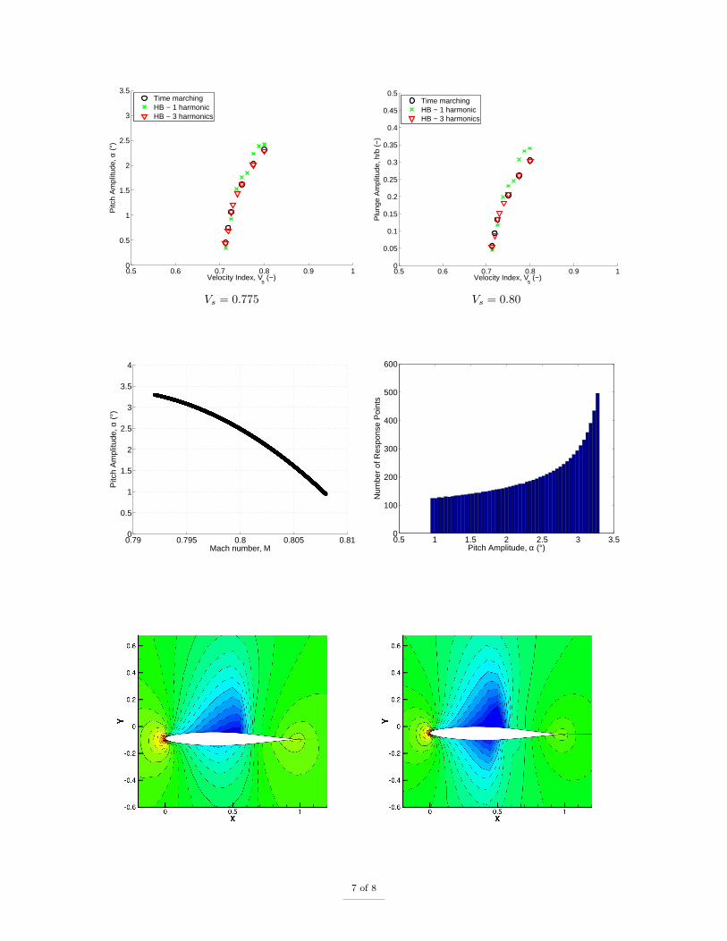
V.A. Pitch/plunge aerofoil

To exercise the method, a two degree-of-freedom, pitch/plunge NACA 64A010 aerofoil is used. The transonicflow, (M∞ = 0.8) is considered to be inviscid. A validation and grid convergence study have been performedreported in reference ?? and a 4000 point grid as shown in fig.V.A was used. The equations of motion aredescribed in eq.26

mh+ Sαα+ khh = −q∞cCl (26)

Sαh+ Iαα+ kαα = −q∞c2Cm (27)

The flutter condition is [ω, Vs] = [0.1089, 0.693] Following Thomas et al.20 the non-dimensional form of

eq.(19) for this problem becomes:

My +1

V 2Ky =

4

πµf (28)

the pitch-plunge aerofoil structural parameters are given by:

M =

[

1 xα

xα r2α

]

, K =

(

ωh

ωα

)2

0

0 r2α

, f =

[

−Cl

2Cm

]

,

y =

h

bα

, V =U∞

√µωαb

with the remainder parameters given in table 1. The plunge direction is represented by h and pitch by αwith the respective frequencies, ωh and ωα, Sα, Iα are the first and second moments of inertia of the aerofoilabout the elastic axis, m is the structure’s mass and b is the half chord, V and U∞ are the reduced andoriginal free stream velocities, respectively.

5 of 8

In addition to the above parameters, the Mach number is set to 0.8 and all calculations are started atan angle of attack of 0◦; the aeroelastic axis distance from the centre chord is set to zero. A variation inpitch and plunge of 0.01◦ and 0.01b are used to perturb the system away from its initial position. Theflutter conditions are obtained from ref.,21 limit-cycle oscillations are reported to occur at [V, µ] = [44, 4400].Figure ??-(a) shows the convergence of the fluid HB system, when the fluid system residual is reduced byeight orders of magnitude, the frequency is recomputed following eq.(25) to drive the structural residual toconvergence, as the structural system is updated, the residual reduces following a staircase pattern, similarto the convergence of the frequency of oscillations.

VI. Conclusions & Outlook

The implementation of a framework to predict limit cycle oscillations was coupled with an implicit HBCFD solver. The application of implicit methods provides faster convergence of the CFD residual by allowingthe use of larger CFL numbers, which was considered a bottleneck for this approach. Initial results for apitch/plunge aerofoil are encouraging and show the potential of this approach to predict nonlinear, periodicaeroelastic instabilities for large and more complex cases.

Acknowledgments

This work was sponsored by the United Kingdom Engineering and Physical Sciences Research Council(grant number EP/K005863/1). The authors gratefully acknowledged this support.

Static unbalance, xα = Sα/mb 0.25

Radius of gyration about elastic axis, r2α = Iα/mb2 0.75

Frequency ratio, ωh/ωα 0.5

Mass ratio, µ = m/πρ∞b2 75

Table 1. Pitch/Plunge Aerofoil Parameters

6 of 8

0.5 0.6 0.7 0.8 0.9 10

0.5

1

1.5

2

2.5

3

3.5

Velocity Index, Vs (−)

Pitc

h A

mpl

itude

, α (

°)

Time marchingHB − 1 harmonicHB − 3 harmonics

0.5 0.6 0.7 0.8 0.9 10

0.05

0.1

0.15

0.2

0.25

0.3

0.35

0.4

0.45

0.5

Velocity Index, Vs (−)

Plu

nge

Am

plitu

de, h

/b (

−)

Time marchingHB − 1 harmonicHB − 3 harmonics

Vs = 0.775 Vs = 0.80

0.79 0.795 0.8 0.805 0.810

0.5

1

1.5

2

2.5

3

3.5

4

Mach number, M

Pitc

h A

mpl

itude

, α (

°)

0.5 1 1.5 2 2.5 3 3.50

100

200

300

400

500

600

Pitch Amplitude, α (°)

Num

ber

of R

espo

nse

Poi

nts

7 of 8

References

1T. E. Noll, J. M. Brown, M. E. Perez-Davis, S. D. Ishmael, G. C. Tiffany, M. Gaier, Investigation of the Helios PrototypeAircraft Mishap, Tech. rep., NASA (2004).

2R. Bunton, C. Denegri, Limit Cycle Characteristics of Fighter Aircraft, Journal of Aircraft 37 (5) (2000) 916–918.3J. Thomas, E. Dowell, K. Hall, C. Denegri, Modeling limit cycle oscillation behavior of the F-16 fighter using a harmonic

balance approach, Tech. rep., AIAA, presented at the AIAA/ASME/ASCE/AHS/ASC Structures, Structural Dynamics, andMaterials Conference, AIAA Paper 2004-1696 (2004).

4P. Beran, N. Knot, F. Eastep, R. Synder, J. Zweber, Numerical Analysis of Store-Induced Limit Cycle Oscillarion, Journalof Aircraft 41 (6) (2004) 1315–1326.

5T. Lieu, C. Farhat, M. Lesoinne, Reduced-order fluid/structure modeling of a complete aircraft configuration, ComputerMethods in Applied Mechanics and Engineering 195 (41–43) (2006) 5730–5742, john H. Argyris Memorial Issue. Part {II}.doi:10.1016/j.cma.2005.08.026.URL http://www.sciencedirect.com/science/article/pii/S0045782505005153

6W. Silva, Identification of Nonlinear Aeroelastic Systems Based on the Volterra Theory: Progress and Opportunities,Nonlinear Dynamics 39 (1-2) 25–62. doi:10.1007/s11071-005-1907-z.URL http://dx.doi.org/10.1007/s11071-005-1907-z

7D. Lucia, P. Beran, W. Silva, Aeroelastic System Development Using Proper Orthogonal Decomposition and VolterraTheory, AIAA Journal 42 (2) (2005) 509–518.

8S. Munteanu, J. Rajadas, C. Nam, A. Chattopadhyay, Reduced-order model approach for aeroelastic analysis involvingaerodynamic and structural nonlinearities, AIAA Journal 43 (3) (2005) 560–571.

9W. Yao, M.-S. Liou, Reduced-Order Modeling for Limit-Cycle Oscillation Using Recurrent Artificial Neural NetworkP-resented at the 14th AIAA/ISSMO Multidisciplinary Analysis and Optimization Conference.

10Hall Kenneth C., Thomas Jeffrey P., Clark W. S., Computation of Unsteady Nonlinear Flows in Cascades Using aHarmonic Balance Technique, AIAA Journal 40 (5) (2002) 879–886, doi: 10.2514/2.1754. doi:10.2514/2.1754.

11A. Gopinath, P. Beran, A. Jameson, Comparative Analysis of Computational Methods for Limit-Cycle OscillationsPre-sented at 47th AIAA/ASME/ASCE/AHS/ASC Structures, Structural Dynamics, and Materials Conference.

12M. Woodgate, K. Badcock, Implicit Harmonic Balance Solver for Transonic Flow with Forced Motions, AIAA Journal47 (4) (2009) 893–901.

13F. Blanc, F.-X. Roux, J.-C. Jouhaud, Harmonic-Balance-Based Code-Coupling Algorithm for Aeroelastic Systems Sub-jected to Forced Excitation, AIAA Journal 48 (11) (2010) 2472–2481.

14M. Woodgate, G. Barakos, Implicit Computational Fluid Dynamics Methods for Fast Analysis of Rotor Flows, AIAAJournal 50 (6) (2012) 1217–1244.

15K. Ekici, K. Hall, Harmonic Balance Analysis of Limit Cycle Oscillations in Turbomachinery, AIAA Journal 49 (7) (2011)1478 – 1487.

16Sicot Frederic, Gomar Adrien, Dufour Guillaume, Dugeai Alain, Time-Domain Harmonic Balance Method for Turboma-chinery Aeroelasticity, AIAA Journal 52 (1) (2014) 62–71, doi: 10.2514/1.J051848. doi:10.2514/1.J051848.

17W. Yao, S. a. Marques, Prediction of Transonic Limit Cycle Oscillations using an Aeroelastic Harmonic Balance Method-Presented at the 44th AIAA Fluid Dynamics Conference, Paper AIAA 2014-2310.

18P. Roe, Approximate Riemann Solvers, Parameter Vectors, and Difference Schemes, Journal of Computational Physics43 (2) (1981) 357–372.

19B. van Leer, Towards the ultimate conservative difference scheme. II. Monotonicity and conservation combined in asecond-order scheme, Journal of Computational Physics 14 (4) (1974) 361–370. doi:10.1016/0021-9991(74)90019-9.URL http://www.sciencedirect.com/science/article/pii/0021999174900199

20J. Thomas, E. Dowell, K. Hall, Nonlinear Inviscid Aerodynamic Effects on Transonic Divergence, Flutter, and Limit-CycleOscillations, AIAA Journal 40 (4) (2002) 638–646.

21D. D. B. R. D. M. S. W. Riveram, J., NACA0012 Benchmark Model Experimental Flutter Results with Unsteady PressureDistributions, Tech. Rep. NASA TM-107581, NASA (1992).

8 of 8