Self-generated limit cycle tracking of the underactuated

HAL Id: lirmm-01723917https://hal-lirmm.ccsd.cnrs.fr/lirmm-01723917

Submitted on 16 Mar 2018

HAL is a multi-disciplinary open accessarchive for the deposit and dissemination of sci-entific research documents, whether they are pub-lished or not. The documents may come fromteaching and research institutions in France orabroad, or from public or private research centers.

L’archive ouverte pluridisciplinaire HAL, estdestinée au dépôt et à la diffusion de documentsscientifiques de niveau recherche, publiés ou non,émanant des établissements d’enseignement et derecherche français ou étrangers, des laboratoirespublics ou privés.

Self-generated limit cycle tracking of the underactuatedinertia wheel inverted pendulum under IDA-PBC

Hassène Gritli, Nahla Khraief, Ahmed Chemori, Safya Belghith

To cite this version:Hassène Gritli, Nahla Khraief, Ahmed Chemori, Safya Belghith. Self-generated limit cycle tracking ofthe underactuated inertia wheel inverted pendulum under IDA-PBC. Nonlinear Dynamics, SpringerVerlag, 2017, 89 (3), pp.2195-2226. 10.1007/s11071-017-3578-y. lirmm-01723917

https://hal-lirmm.ccsd.cnrs.fr/lirmm-01723917

https://hal.archives-ouvertes.fr

Noname manuscript No.(will be inserted by the editor)

Self-generated limit cycle tracking of the underactuated inertia wheelinverted pendulum under IDA-PBC

Hassene Gritli · Nahla Khraief · Ahmed Chemori · Safya

Belghith

Received: date / Accepted: date

Abstract This paper deals with the tracking approach of a self-generated stable limit cycle for an underac-tuated mechanical system: The Inertia Wheel Inverted Pendulum (IWIP). Such system is subject to unilat-eral constraints limiting its swing motion. It is known that an Interconnection and Damping Assignment-Passivity Based Control (IDA-PBC) can be employed to control such pendulum to its upright position. Inthis work, we briefly show first that the IWIP can generate a stable period-1 limit cycle through a Hopfbifurcation by varying some gain parameter of the IDA-PBC. Thus, such self-generated limit cycle is usedas a reference trajectory, which is chosen to be tracked by the IWIP. To achieve the tracking problem, asupplementary control input is added. Such tracking problem is reformulated as an asymptotic stabilizationof the tracking error. Our fundamental approach hinges mainly on the use of the S-procedure to introducethe unilateral constraints, and the Schur complement and the matrix inversion lemma to transform BilinearMatrix Inequalities (BMI) into Linear Matrix Inequalities (LMI). Several simulations have been presentedto corroborate the mathematical results and to show the efficiency of the proposed tracking scheme of theself-generated stable limit cycle of the controlled IWIP, even if it is subject to external disturbances, or inthe presence of uncertainties in the friction parameters.

Keywords Inertia wheel inverted pendulum · Hopf-bifurcation · Limit cycle · Unilateral constraint ·S-procedure · BMI · LMI

1 Introduction

Equilibrium points and limit cycles are known to be common solutions for almost all continuous-timenonlinear dynamical systems. Limit cycles model dynamical systems that exhibit self-sustained oscillationsfor some set of parameters. Thus, a self-excited system exhibits the property to generate steady stateoscillations (limit cycles) even in the absence of external periodic forcing [1–3]. Some examples of dynamicalsystems that exhibit a self-excited oscillation are beating of a heart, rhythms in body temperature, hormonesecretion, chemical reactions, vibrations in bridges and airplane wings, inverted pendulums, the Van der Poloscillator, the Duffing oscillator, biped robots, etc. [4–7] (see also [8, 9] for further examples). In general, self-oscillators give a regular output robustly: they approach the same limit cycle regardless of initial conditionsand transient perturbations [2]. In addition, limit cycles are generated through bifurcations, among whichthe most popular and important one is the Hopf bifurcation [1, 4, 6, 10], which occurs for autonomous

H. Gritli⋆

Institut Superieur des Technologies de l’Information et de la Communication,Universite de Carthage, 1164 Borj Cedria, Tunis, Tunisia⋆E-mail: [email protected]

H. Gritli · N. Khraief · S. BelghithLaboratoire Robotique, Informatique et Systemes Complexes (RISC–LR16ES07),Ecole Nationale d’Ingenieurs de Tunis, Universite de Tunis El-Manar,BP. 37, Le Belvedere, 1002 Tunis, Tunisia

A. ChemoriLIRMM, University of Montpellier 2, CNRS, 161 rue Ada, 34392 Montpellier, France

2 Gritli et al.

dynamical systems. Such local bifurcation gives rise to the birth of a limit cycle via a stable equilibriumpoint. This limit cycle can be either stable or unstable. In the former case, the Hopf bifurcation is super-critical. However, in the latter case, the Hopf bifurcation is sub-critical [4, 7, 10].

Recently, the interest in the control problem of underactuated mechanical systems has increased dueto their complexity and applications. Several kinds of underactuated mechanical systems exist in literaturesuch as the double inverted pendulum, the rotational inverted pendulum, the Furuta pendulum, the cart-pendulum system, the wheeled inverted pendulum, the flywheel inverted pendulum, among others [11–18].In general, inverted pendulums are very suitable to illustrate many ideas in automatic control of nonlinearsystems. A special underactuated mechanical system is the Inertia Wheel Inverted Pendulum (IWIP),which has two degrees of freedom with only one actuator [19, 20]. Such underactuated mechanical systemhas attracted the attention of several researchers in robotics and control system engineering where severalcontrol strategies have been designed (see for example [11–17] and references therein). The most recognizedworks are those based on the energy point-of-view. The general control strategy is to swing the underactuatedmechanical system, such as the Acrobot, the Pendubot, the IWIP, the Tora system, the Furuta pendulum,in order to bring/stabilize it to the desired (upright) position.

1.1 Literature review

The control objective of the IWIP is to stabilize it at the upright position, namely around the unstableequilibrium point. Many works related to this topic have been proposed. The passivity-based control withsaturated control input based on the feedback linearization was introduced in [19, 20]. Olfati-Saber [21, 22]employed the standard backstepping procedure. Fantoni and Lozano [15] introduced the total energy storedin the system in order to design a nonlinear swinging-up control strategy. Ramamoorthy and Kuipers [23]developed an approach that uses switching between multiple controllers to robustly stabilize the uprightequilibrium. The same problem was solved in [24] with a single output feedback controller, which wasdesigned using a passivity-based method. Moreover, Ortega et al. [25] used the Interconnection and DampingAssignment-Passivity Based Control (IDA-PBC) (see [26] for a survey) for the asymptotic stabilization of theIWIP around its upward position. They formulated the designed controller for Port-Controlled Hamiltonianmodels [27]. In [28, 29], the undesirable effects of the damping force was taken into account in the controlstrategy. Qaiser et al. [30] presented a novel nonlinear controller design by fusing the dynamic surface controland the control Lyapunov function method. In addition, Touati and Chemori [31] proposed a generalizedpredictive control scheme. They proved via experimentation the robustness of such controller against externaldisturbances and uncertainties in the inertia parameters of the IWIP. Moreover, Olivares and Albertos[32, 33] used a simple PID controller and an observer-based state feedback controller by linearizing thedynamics around the unstable equilibrium point. Recently, Khraief et al. [34] employed the IDA-PBC for theasymptotic stabilization of the underactuated IWIP around its unstable upward position in the presence ofexternal disturbances. Some sufficient stability conditions on matched and unmatched disturbances were alsopresented. Moreover, in [35], Khraief et al. enhanced the IDA-PBC by combining it with an adaptive controltechnique to estimate controller gains. Ryalat and Laila [36] used a simplified IDA-PBC by consideringfriction parameters. They estimated the friction parameters in order to calculate the friction compensationterm. Some other works were realized on the control of inverted pendulums [17, 37–40].

Another interesting and challenging task with the IWIP is the stabilization of periodic motions. Authorsin [41–46] developed a (quasi-continuous) high(second)-order sliding mode control to solve the trackingcontrol problem for the IWIP. These authors developed a reference model (trajectory) based on a two-relaycontroller, which was introduced to produce oscillations where the desired amplitude and frequency werereached by choosing the control gains properly. The two-relay controller consists of two relays switched bythe feedback received from a linear or nonlinear system, and represents a new approach to the self-generationof periodic motions in underactuated mechanical systems and hence to design a (robust) tracking controller[45]. The design procedures for the two-relay control and hence the periodic oscillations developed byAguilar and his co-workers were based on three different methodologies, namely the describing-functionmethod, the Poincare maps, and the locus-of-a perturbed-relay-system method. Authors in [44] consideredthe viscous friction affecting the active joint. Another approach for stabilizing periodic motions aroundthe upper equilibrium of the IWIP was presented by [47]. Furthermore, a constructive method introducedin [48–50] was applied for the generation of periodic motions in underactuated nonlinear systems throughvirtual holonomic constraints and for orbital stabilization via a partial feedback transformation. Gruber andHofbaur [51] employed the same method for planning periodic motions and designing a stabilizing controllerbased on a thorough analysis of the dynamics transversal to the resulting limit cycle. In addition, Andary et

al. [52] proposed a control approach dedicated to stable limit cycle generation for the IWIP. The proposed

Limit cycle tracking of the IWIP under IDA-PBC 3

approach was based on partial nonlinear feedback linearization and dynamic control for optimal periodicreference trajectories tracking. The feedback controller presented in [52] is enhanced in [53, 54] to handleconstant disturbances in limit cycle tracking by using online iterative estimation of an equivalent disturbancewhich is easily compensated by adding the estimated value to the output of the system. Moreover, Zayane-Aissa et al. [55] introduced a high order sliding mode structure to solve the problem of trajectory trackingproblem of the IWIP in presence of unknown input perturbation. Aguilar-Ibanez et al. [56] used the statefeedback controller to ensure the tracking of a limit cycle characterized in terms of the feedback-linearizablesingle-input affine nonlinear dynamical systems and, as an application, of the IWIP.

Some analysis of the IWIP under control have been considered in literature using bifurcation theory.Alonso et al. [57] employed the bifurcation theory to classify different dynamical behaviors arising in theIWIP subject to bounded continuous-state-feedback control law. To limit the maximum amplitude of thecontrol action, the control law is subject to a smooth saturation function, which was introduced first in [58]in order to stabilize the IWIP at the inverted position. Alonso et al. [57] showed that the global dynamicsof the IWIP changes from a stable equilibrium point to a stable limit cycle via a Hopf bifurcation as certaincontrol gains change. A similar work was realized on the Furuta pendulum by analyzing the Hopf bifurcation[59]. Recently, Nikolov and Nedev [60] analyzed bifurcation and dynamic behavior of the IWP with boundedcontrol by means of the theory of Poincare-Andronov-Hopf.

Moreover, in the literature, there are several design methods of the feedback controller using the LinearMatrix Inequality (LMI henceforth) approach [61], such as the state feedback control, the static outputfeedback control, the dynamic output feedback control, the observer-based feedback control, among others(see for example [62] and references therein). However, most control synthesis problems cannot be writtenin LMI setting, while in terms of a more general form known as a Bilinear Matrix Inequality (BMI).Computations over BMI constraints are known as NP-hard and difficult to obtain a solution. There areseveral approaches and different relaxed synthesis conditions proposed for conducting the BMIs into LMIs.Generally, all these approaches use for example the Schur complement Lemma, the Finsler Lemma, theprojection Lemma, the Young relation, among others [61]. A brief review on the state feedback control designusing LMI methods for continuous-time linear systems was presented in [63]. Some extensions and numericalcomparisons between several state feedback stabilization conditions were also provided. Furthermore, anew extended LMI characterization for the state feedback control of continuous-time linear systems withuncertainty was presented in [64].

1.2 Motivations

The motivations of studying and controlling the underactuated IWIP mainly stem from five facts:

1. In spite of various efforts on the stabilization of the IWIP, a considerable attention is still required forthe generation of stable periodic oscillation for the IWIP and synthesis of a feedback control law to trackit. In this present paper, we use the theory of bifurcations to generate a stable one-periodic limit cycleby means of the Hopf bifurcation by varying some control parameter.

2. According to [34, 35, 52–54], the motion of the IWIP is constrained. Indeed, the planar swing motionof the pendulum body is subject to unilateral contacts (constraints) [65], for which its angular positionreaches a certain maximum/minimum value at standstill. Olivares and Albertos [33] worked with aphysical device having such constraints. To the best of authors’ knowledge, no previous work in theliterature has been dealt with such constrained dynamics. Only the free swing motion of the IWIP wasprovided and analyzed. In this work, the dynamics of the IWIP is subject to external disturbances andstate constraints. Such state constraints are taken into account for the first time in the present workand play an important role in the design of the tracking controller for the self-generated limit cycle.

3. The dynamics of the IWIP is a simple class of nonlinear systems with trigonometric nonlinearities, whichcan occur in robotic applications, such as the single-link flexible robot manipulator [66, 67] and the pitchdynamics of a simplified helicopter model [68, 69], and other nonlinear systems.

4. Moreover, the IWIP was known as a testbed underactuated mechanical system used to design newcontrollers. It can be used for example to control the simplest model of a walking robot leg [70, 71].Authors in [70, 71] used a liner inverted pendulum controlled via a flywheel model in the sagittal plane[70] and in the 3D [71] in order to generate angular momentum. They showed that such flywheel-basedinverted pendulum can effectively describe the reaction of human if perturbed by external force whilewalking and standing. A related approach was employed also in [72] for the SURENA III humanoidrobot using the linear inverted pendulum with a flywheel. Actually, the effect of angular momentumof the upper-body, especially the torso and arms, of a biped robot can play an important role in push

4 Gritli et al.

recovery and hence walking over rough terrain. The effect can be embedded by considering the upperbody as a flywheel that can be actuated directly [73].

5. Bipedal robot control techniques implementing self-clocking properties as presented in [74] have desirableproperties, like the ability to drive the robot step with respect to its own geometry. In [75, 76], themotivation of adding a disk to the legged robot dynamics is to produce a desirable effect, a desired zeromoment point, and hence to design the geometry of the walking step. A related work was presented alsoin [77] where authors employed the same method of reference trajectory generation introduced in [53] forthe IWIP. In addition, an adaptive control of a gyroscopically stabilized pendulum and its application toa single-wheel pendulum Robot was presented in [78] using the conventional reaction wheel pendulummodel.

1.3 Objective and contributions

In this paper, we will use the IDA-PBC introduced in [34, 35] to control the IWIP at its upright position.Thus, we will (briefly) show that the nonlinear dynamics of the IWIP under the IDA-PBC demonstratesa stable limit cycle through a super-critical Hopf bifurcation as some control gain of the IDA-PBC varies.Indeed, we will present stability conditions of the controlled equilibrium point with respect to the controlgains. Moreover, we will develop conditions for the presence of the Hopf bifurcation and then of periodicoscillation. Furthermore, stability of these periodic oscillations is investigated numerically by means of thefirst Lyapunov value. Thus, we will show that for some critical control gains, the controlled dynamics of theIWIP exhibits both sub-critical and super-critical Hopf bifurcations. At this last critical bifurcation point,the IWIP under the IDA-PBC experiences a stable period-1 limit cycle. However, the existence of multipleattractors, and hence stable limit cycles, in the parameter space is a common phenomenon in nonlinearsystems. Thus, depending on initial conditions, new limit cycles or other kinds of attractors (such as chaoticor quasi-periodic attractor) can be observed besides the already known, i.e. the stable limit cycle. Each limitset (attractor) is defined by its basin of attraction. For the underactuated IWIP as a physical system, itis difficult to provide the adequate initial conditions in order to guarantee that the IWIP converges to thedesired stable limit cycle. Moreover, if we assume that the system trajectory converges to the desired limitcycle for all sets of initial conditions, the second problem lies in the speed (or time) of convergence itself. Inthis work, we show that for an initial condition almost identical to the desired one and for some value of thecontrol gain, the trajectory of the IWIP under the IDA-PBC requires much time to converge and hence tostabilize around its own limit cycle. Moreover, we show that the two periodic motions are not synchronized.Then, the main contribution in this paper is to solve this problem for the underactuated IWIP by trackingthe desired generated stable limit cycle. Our methodology lies in the tracking of a reference model as agenerator of the desired limit cycle. Such reference model is the underactuated nonlinear dynamics of theIWIP under the IDA-PBC. For some set of control gains, such dynamics exhibits a stable period-1 limitcycle for a predefined initial condition. The objective is that the (physical) IWIP system tracks the desiredreference model, which generates the desired stable period-1 limit cycle. To achieve this goal, our approachis to add a new control input (a limit-cycle tracking control law) to the controlled IWIP system. Thus, thelimit cycle tracking problem will be reformulated as the stabilization problem of the tracking error.

According to [34, 35, 52–54], all the states of the physical device of the IWIP are available for directmeasurement. Thus, in this paper, we will adopt a state-feedback control law to solve the self-generatedlimit cycle tracking problem of for the underactuated IWIP. Moreover, the constraints in the dynamics ofthe IWIP are introduced. Actually, two main keys are used in order to solve the tracking problem. Thefirst key is the use of the S-procedure [61] in order to reduce the conservatism of the classical Lyapunovapproach. The S-procedure gives in fact the possibility of reducing the field of verification conditions in auseful subspace Ω, that is from R to some Ω ⊂ R. For the IWIP, the useful subspace is that limited with theunilateral constraints. The problem of finding stability conditions of the tracking error will be recast as anonconvex optimization problem based on BMIs. The second key for achieving the tracking problem is theuse of the Schur complement [61] and also the matrix inversion lemma in order to transform the BMIs intoLMIs, which will be used to allow a numerical solution of the problem. We will show the effectiveness ofthe developed controller for the tracking of the desired self-generated period-1 limit cycle. We will achieveseveral simulations: a nominal system without uncertainties in the friction parameters and disturbance, asystem under uncertain friction parameters, and a system subject to constant and randomly time-varyingexternal disturbances.


1.4 Structure of the paper

The rest of the paper is organized as follows. In Section 2, a brief description of the IWIP, its dynamicsand the IDA-PBC are presented. Self-generation of a stable limit cycle through the Hopf bifurcation isbriefly discussed also in this section. Problem formulation of the self-generated limit cycle tracking of theunderactuated IWIP under the IDA-PBC is described in Section 3. Section 4 deals with the design of thetracking control law using the framework of LMI. Some well-known preliminaries for solving the asymptoticstabilization problem are provided first. Transformation of the BMIs into LMIs is realized in this sectiontoo. Section 5 is dedicated to simulation results. Concluding remarks are drawn in Section 6. Finally, ananalysis of the dynamics of the IWIP under the IDA-PBC in order to demonstrate existence of the Hopfbifurcations and then generation of the stable limit cycle is given in Appendix.

2 The underactuated inertia wheel inverted pendulum under the IDA-PBC

2.1 Description of the underactuated inertia wheel inverted pendulum

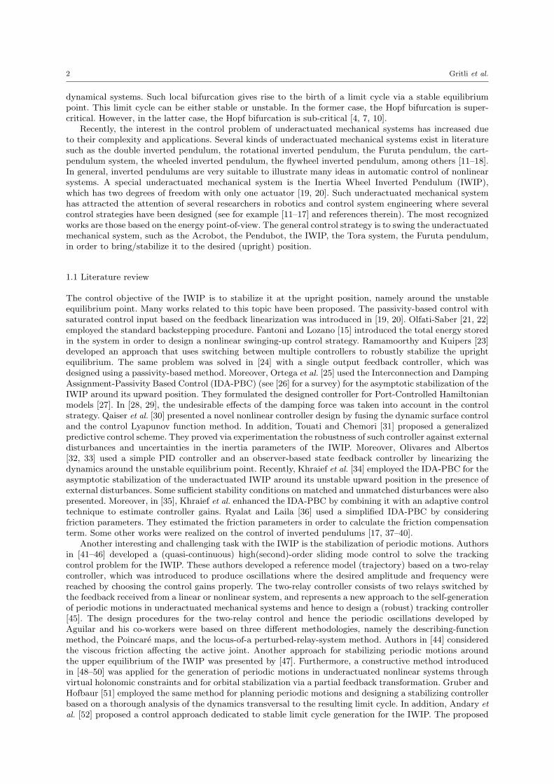
The underactuated inertia wheel inverted pendulum (IWIP) (Fig. 1) consists of an inverted pendulumpivoting on a frictionless point with a rotating wheel on the top. Its mechanical structure is sketched inFig. 2. In Fig. 2, the joint between the frame and the pendulum body is unactuated (passive), while thejoint between the body and the inertia wheel is actuated (active) via the control input u. The inertia wheelis free to rotate about an axis parallel to the axis of rotation of the pendulum. Hence, the IWIP is a planarmechanical system. This electromechanical system is controlled by a DC motor actuating the inertia wheel(see [31] for further descriptions of this system). The motor torque produces an angular acceleration ofthe rotating wheel, which generates a torque acting on the passive joint of the pendulum by means of thedynamic coupling. Therefore, this passive joint can be controlled through the acceleration of the inertiawheel. The dynamic parameters of the IWIP and its description are given in Table 1. In Fig. 2, θ1 is theangular position of the pendulum body, whereas θ2 is the rotation angle of the inertia wheel. The motionof the pendulum is subject to unilateral constraints defined as:

Ω = θ1 ∈ R : −σ ≤ θ1 ≤ σ . (1)

where σ = θ1max. According to [53], the pendulum angle value is approximately ±10 at standstill (i.e. atthe pendulum stop). Then, σ = 10.

In this work, we ignore the collision effect of the pendulum body with the stop.

Fig. 1 Physical device of the underactuated inertia wheel inverted pendulum.

2.2 Dynamic model of the IWIP

The dynamic model of the underactuated IWIP is obtained by application of the Euler-Lagrange formulation[79]. Based on [34, 35, 53], the mathematical model of the IWIP augmented with viscous frictions in theactive and passive joints and with disturbances is described by:

6 Gritli et al.

Fig. 2 Schematic representation of the underactuated inertia wheel inverted pendulum.

Table 1 Important dynamic parameters of the underactuated inertia wheel inverted pendulum.

Symbol Description Value Unit

m1 Pendulum mass 3.228 Kgm2 Wheel mass 0.33081 Kgl1 Pendulum center of mass position 0.06 ml2 Wheel center of mass position 0.044 mI1 Pendulum inertia 0.0314 Kg.m2

I2 Wheel inertia 4.176e− 4 Kg.m2

[I + I2 I2I2 I2

] [θ1θ2

]−[bg sin (θ1)

0

]+

[δ1θ1δ2θ2

]=

[01

]u+

[10

]ζ (2)

where θ1 and θ2 correspond to the velocity of the pendulum body and the inertia wheel, respectively; θ1and θ2 are their corresponding accelerations; u is the torque applied by the motor on the inertia wheel; ζ isthe external disturbing torque applied to the pendulum; I = m1l

21 +m2l

22 + I1; b = m1l1 +m2l2; δ1 and δ2

represent, respectively, the friction coefficients of the passive and the active articulations.According to [31, 34, 35, 53], the physical device of the IWIP system (Fig. 1) was mechanically designed

so as to minimize the effects of viscous frictions. Thus, in this study the frictions of the active and passivejoints, i.e. δ1 and δ2, are so low that we have neglected. Then, in the sequel of this work, we consider thenominal system, that is without friction (δ1 = δ2 = 0). Moreover, the torque ζ is considered to be zero,that is the nominal system is not subject to external disturbing torque. Hence, the nominal dynamics ofthe IWIP is described as follows:[

I + I2 I2I2 I2

] [θ1θ2

]−[bg sin (θ1)

0

]=

[01

]u (3)

Remark 1 The effect of the friction coefficients δ1 and δ2 and the external disturbance ζ on the trackingproblem of the self-generated limit cycle of the underactuated IWIP under IDA-PBC will be analyzed insection 5 through numerical simulations. The damping coefficients δ1 and δ2 will be considered as twouncertain parameters.

Authors in [25, 34, 35] introduced the following change of coordinates:[q1q2

]=

[1 01 1

] [θ1θ2

](4)

Thus, using (4), the dynamics in (3) can be rewritten like so:


[I 00 I2

] [q1q2

]−[bg sin (q1)

0

]=

[−11

]u (5)

The model (5) can be rewritten through Hamilton’s equations of motion as [24, 34, 35]:q1q2p1p2

=

p1

Ip2

I2bg sin (q1)− u

u

(6)

where p1 = Iq1 and p2 = I2q2 [25, 34, 35].

2.3 The IDA-PBC controller

According to [25, 27, 34, 35], the Interconnection and Damping Assignment-Passivity Based Control (IDA-PBC) is expressed as follows:

u = γ sin (q1) + k1q1 + k2q2 + k3p1 + k4p2 (7)

with ki are control gains and ki > 0, ∀i = 1, 2, 3, 4, and γ > bg.In the expression of the IDA-PBC u (7), the first three terms reveal the energy shaping control to assign

the equilibrium. However, the last two terms inject damping to the pendulum body and the inertia wheelto achieve asymptotic stability. In [34, 35], the control gains were calculated and selected as: γ = 6.1284,k1 = 1.0367, k2 = 0.0011, k3 = 16.62 and k4 = 3.4640. With these parameters and under the dynamicnonlinear output feedback IDA-PBC (7), the underactuated IWIP was stabilized in its upward equilibriumpoint.

2.4 Self-generation of a stable limit cycle through Hopf bifurcation

By introducing (7) in (6), the closed-loop dynamics of the underactuated IWIP is given by:x1x2x3x4

=

x3Ix4I2

(bg − γ) sin (x1)− k1x1 − k2x2 − k3x3 − k4x4γ sin (x1) + k1x1 + k2x2 + k3x3 + k4x4

(8)

with x =[x1 x2 x3 x4

]T=

[q1 q2 p1 p2

]T.

It is straightforward to demonstrate that the equilibrium point of the nonlinear system (8) is expressedby:

xeq =

kπ

−kπ k1

k2

00

(9)

where k ∈ Z.Moreover, as the controlled IWIP is under the state constraints (1), then the only equilibrium point is

the origin. The Jacobian matrix around the equilibrium point xeq (we consider only the upright position)of the closed-loop nonlinear system (8) is defined as follows:

J =

0 0 1

I 00 0 0 1

I2bg − γ − k1 −k2 −k3 −k4

γ + k1 k2 k3 k4

(10)

It is worth mentioning that as the only equilibrium point of the system (8) is the origin, then the onlyway for which such equilibrium point will lose its stability is through the Hopf bifurcation. Indeed, byvarying the control gains ki and by analyzing the eigenvalues of the Jacobian matrix (10), the controlledequilibrium point xeq loses its stability at some critical values of the gains ki. At these critical values, sayingkci , the closed-loop nonlinear dynamics (8) undergoes a Hopf bifurcation, at which there is a creation of

8 Gritli et al.

either a stable limit cycle or an unstable one. Since the unstable limit cycle (as an unstable solution innonlinear dynamics) is not observable, and hence only the stale limit cycle has physical means.

We recall that the main objective of this paper is the design of a tracking controller of some self-generated stable limit cycle of the IWIP for some set of gain parameters ki. Then, stability investigation ofthe equilibrium point xeq with respect to the parameters ki, existence demonstration of the Hopf bifurcationand then limit cycles and its stability are not developed in this part and only presented in Appendix 1. Amore detailed work dealing with this subject will be developed in another paper.

According to Appendix 1, by fixing the control gains k1, k2 and k3, and by varying the remaining onek4, the Hopf bifurcation occurs at two critical values of k4: k

c4,1 ≈ 0.8716 and kc4,2 ≈ 27.1977. For kc4,1, the

Hopf bifurcation was found to be sub-critical and hence only unstable limit cycles were born. However, forthe second critical value kc4,2, the Hopf bifurcation is super-critical and accordingly a period-1 stable limitcycle was born. For k4 lying between kc4,1 and kc4,2, the equilibrium point is asymptotically stable.

In order to investigate the dynamic behavior of the IWIP as the parameter k4 varies, we used bifurcationdiagrams where some measure (for example x1, i.e. θ1) of the solution state is plotted against the parameterk4. Moreover, as the origin is the only equilibrium point, then we will focus on the generated stable limitcycle through the super-critical Hopf bifurcation. Figure 3 shows a bifurcation diagram of the controlledunderactuated IWIP as the parameter k4 varies. For k4 < kc4,2, the controlled IWIP converges to the stableequilibrium point (marked as SEP in Fig. 3). As k4 increases, the SEP loses its stability and hence becomesan unstable focus (indicated as UEP) via the Hopf bifurcation (marked as HB in Fig. 3). At the criticalpoint kc4,2 ≈ 27.1977, the controlled IWIP experiences a stable period-1 limit cycle. As k4 increases, theamplitude of this limit cycle grows rapidly (according to a certain square function). Thus, the stable limitcycle persists for a small interval of the control gain k4, i.e. k

c4,2 < k4 < 30.

Fig. 3 Bifurcation diagram displaying the steady solutions of the closed-loop unconstrained IWIP as the control gain k4varies. This diagram shows the maximum angular position, θ1 = q1 = x1, of the pendulum body versus k4.

Figure 4(a) (resp. Figure 4(b)) reveals some stable period-1 limit cycles in the phase portrait of thependulum (resp. the inertia wheel) for some values of the parameter k4. The smallest limit cycle is depictedfor k4 = 27.201 and the largest one is plotted for k4 = 27.25. For k4 = 27.201, the pendulum body reachesthe angular position about 9. Whereas, for k4 = 27.25, the maximum angular position of the pendulumis about 30. It is obvious how the limit cycle of the pendulum grows in terms of amplitude as the controlgain k4 increases slightly.

We emphasize that stable limit cycles in the bifurcation diagram in Fig. 3 are computed using an iterativemethod called as the Poincare shooting method [80] by defining first a Poincare section:

PS =x ∈ R4×1, h(x) = x3 = CSx = 0, CS x < 0

, (11)

with CS =[0 0 1 0

]. The condition CS x < 0 in (11) is added to ensure that the flow intersects the

hyperplane defined by CSx = 0 in only one direction.It is worth noting that for a stable period-1 limit cycle, the flow starting from its fixed point x⋆ located

on the Poincare section (11) returns to the Poincare section and intersects it in the same fixed point x⋆.The return time, say τr, represents the time between two successive intersections with the Poincare section


(a) (b)

Fig. 4 Limit cycles of the pendulum for some values of the control gain parameter k4. From inside to outside: k4 = 27.201,k4 = 27.21, k4 = 27.22 and k4 = 27.25. (a) shows the limit cycles of the pendulum body, whereas (b) displays the limitcycles of the inertia wheel.

and it defines the period of the stable period-1 limit cycle. We note that the return time is calculated whenintegrating the nonlinear dynamics (8) and hence locating the fixed point x⋆ through the Shooting method.For example, the smallest stable limit cycle, i.e. for k4 = 27.201, has a self-sustained oscillation period about0.5900 [s]. However, for k4 = 27.25, the self-sustained oscillation period is about 0.5989 [s]. We stress thatthe first value of the period (i.e. for k4 = 27.201) is almost identical to that calculated theoretically throughexpression (91) (see Appendix 1).

3 Problem formulation

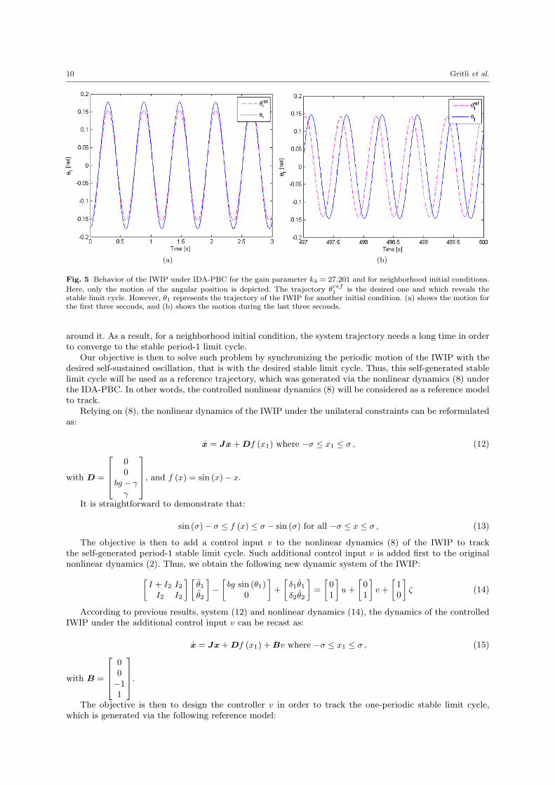
We emphasize that the bifurcation diagram in Fig. 3 and the limit cycles in Fig. 4 are plotted withouttaking into account the constraints on the motion of the pendulum body of the IWIP. We note that in someprevious papers such as that of Ortega and his co-workers, the motion of the IWIP was totally free and noconstraint was considered. Then, if we consider here that the motion of the IWIP is subject to unilateralconstraints defined by (1) and as presented in Fig. 1 and Fig. 2, some limit cycles in Fig. 3 and in Fig. 4will not be considered. The maximum angular position that can be reached by the pendulum body is about10. Then, in the sequel of this paper, we will interest only in the first stable limit cycle in Fig. 4(a), i.e.for k4 = 27.201. This stable limit cycle will be used as a reference trajectory, which was generated viathe nonlinear dynamics (8) under the IDA-PBC. The initial condition of such limit cycle is chosen to be:(θr1(0), θ

r2(0), θ

r1(0), θ

r2(0)

)= (−8.8579, 23.0117 rad, 0.0066 rad/s,−0.9831 rad/s).

We want to show the motion of the IWIP under the IDA-PBC for the same gain parameter k4 = 27.201and for another initial condition:

(θ1(0), θ2(0), θ1(0), θ2(0)

)= (−10, 0, 0 rad/s, 0 rad/s). The choice of θ1(0)

is motivated by the physical properties of the IWIP since simulation is started from the rest position atstandstill, for which θ1(0) = ±10. Here, we chosen θ1(0) = −10 in order that such initial position of thependulum body is almost identical to that of the desired one θr1(0). Figure 5 shows the temporal evolutionof both the desired (reference) angular position θr1 and the angular position θ1 of the pendulum body. Thenumerical simulation was achieved for 500 [s]. Figure 5(a) reveals behavior of the IWIP during the first threeseconds, whereas Fig. 5(b) depicts the motion during the last three seconds. It is obvious that for almosttwo identical initial positions of the pendulum body, the motion of the IWIP diverges progressively in timeand the IWIP becomes in phase lag with respect to the reference. Furthermore, even after the stabilizationof the motion of the IWIP, the resulting behavior is found to be completely different to the desired one,where the two motions are not synchronized.

It is worth noting that such result is very meaningful from chaos and bifurcation theory. Indeed, fork4 > kc4,2 the limit set is the stable period-1 limit cycle. By decreasing the value of the bifurcation parameterk4, one among the eigenvalues of the Jacobian matrix of the Poincare map associated to the stable limit cyclebecomes very near to the boundary of the unit circle. Thus, robustness of the stable period-1 stable limitcycle towards perturbations decreases. Hence the limit cycle becomes very sensitive to weak perturbation

10 Gritli et al.

(a) (b)

Fig. 5 Behavior of the IWIP under IDA-PBC for the gain parameter k4 = 27.201 and for neighborhood initial conditions.

Here, only the motion of the angular position is depicted. The trajectory θref1 is the desired one and which reveals thestable limit cycle. However, θ1 represents the trajectory of the IWIP for another initial condition. (a) shows the motion forthe first three seconds, and (b) shows the motion during the last three seconds.

around it. As a result, for a neighborhood initial condition, the system trajectory needs a long time in orderto converge to the stable period-1 limit cycle.

Our objective is then to solve such problem by synchronizing the periodic motion of the IWIP with thedesired self-sustained oscillation, that is with the desired stable limit cycle. Thus, this self-generated stablelimit cycle will be used as a reference trajectory, which was generated via the nonlinear dynamics (8) underthe IDA-PBC. In other words, the controlled nonlinear dynamics (8) will be considered as a reference modelto track.

Relying on (8), the nonlinear dynamics of the IWIP under the unilateral constraints can be reformulatedas:

x = Jx+Df (x1) where −σ ≤ x1 ≤ σ , (12)

with D =

00

bg − γ

γ

, and f (x) = sin (x)− x.

It is straightforward to demonstrate that:

sin (σ)− σ ≤ f (x) ≤ σ − sin (σ) for all −σ ≤ x ≤ σ , (13)

The objective is then to add a control input v to the nonlinear dynamics (8) of the IWIP to trackthe self-generated period-1 stable limit cycle. Such additional control input v is added first to the originalnonlinear dynamics (2). Thus, we obtain the following new dynamic system of the IWIP:[

I + I2 I2I2 I2

] [θ1θ2

]−[bg sin (θ1)

0

]+

[δ1θ1δ2θ2

]=

[01

]u+

[01

]v +

[10

]ζ (14)

According to previous results, system (12) and nonlinear dynamics (14), the dynamics of the controlledIWIP under the additional control input v can be recast as:

x = Jx+Df (x1) +Bv where −σ ≤ x1 ≤ σ , (15)

with B =

00−11

.The objective is then to design the controller v in order to track the one-periodic stable limit cycle,

which is generated via the following reference model:


xr = Jxr +Df (xr1) where −σ ≤ xr1 ≤ σ , (16)

Remark 2 Relying on the dynamics (2) of the underactuated IWIP with parametric uncertainties in thetwo friction coefficients δ1 and δ2 and subject to the external disturbance ζ, the IDA-PBC u in (7) andaccording to the system (15), the state space representation of the controlled IWIP under the parametricuncertainties and the external disturbance can be reformulated as follows:

x = Jx+Df (x1) +Bv + Jx+ Dζ where −σ ≤ x1 ≤ σ , (17)

where J =

0 0 0 00 0 0 0

0 0 − δ1+δ2I

δ2I2

0 0 δ2I − δ2

I2

and D =

0010

.Thus, our goal is to design the new control law v such that the constrained nonlinear system (15) of

the controlled IWIP tracks the reference model (16). The tracking error, e = x−xr, between the nonlineardynamics (15) and the reference model (16) is defined as:

e = Je+D (f (x1)− f (xr1)) +Bv where −2σ ≤ e1 ≤ 2σ , (18)

with e1 = x1 − xr1.Therefore, our approach for achieving the tracking problem lies in the design of the control law v

stabilizing the tracking error of the nonlinear system (18), which is the objective of the next section.

Remark 3 The nonlinear dynamics (12) of the IWIP is under state constraints in which the motion ofpendulum or the state x1 = θ1 evolves in a small region (1) defined as |x1| ≤ 10. Moreover, the nonlinearterm f (x1) presented in the dynamics of the IWIP depends only on the state x1, f (x1) = sin (x1) − x1.Thus, it is possible to use the approximated linear model instead of the nonlinear model to solve the trackingcontrol problem. In this case, we will have f (x1) = 0 since sin (x1) ≈ x1. Hence, the error dynamics in (18)becomes

e = Je+Bv where −2σ ≤ e1 ≤ 2σ (19)

It is worth to note that there is no remarkable difference between the obtained results using the nonlinearsystem (18) or the linear system (19). However, the strategy developed in this work for the controllersynthesis by considering the nonlinear dynamics (18) can be applied for more general constrained nonlinearsystems for which the states evolve in a large region as for the case of the single-link rotary flexible jointrobot studied in [67].

4 Design of the tracking control law

The tracking control law is adopted to be defined like so:

v = −k2e2 + w (20)

with k2 is the control gain in the IDA-PBC (7), e2 = x2 − xr2, and w is an auxiliary tracking control law.By substituting expression of v in the dynamics (18), it follows that the second state variable e2 does

not affect any other variable. Therefore, there is no interest on its evolution and hence it can be discarded.Then, the nonlinear dynamics (18) can be simplified as:

˙e = Ae+ D (f (x1)− f (xr1)) + Bw where −2σ ≤ e1 ≤ 2σ , (21)

with e =[e1 e3 e4

]T, A =

0 1I 0

bg − γ − k1 −k3 −k4γ + k1 k3 k4

, D =

0bg − γ

γ

, and B =

0−11

.Thus, the tracking problem will be recast as an asymptotic stability problem of the tracking error e of

the nonlinear system (21) by means of the control law w. To achieve such asymptotic stability, we adopt asimple state-feedback linear control law as:

w =

Ke whenever ∥e∥ > ϵ

0 elsewhere(22)

12 Gritli et al.

where K is a constant gain matrix which will be obtained later, and ϵ is very small positive constant.Substituting this control law into (21), it yields the new closed-loop dynamics:

˙e =(A+ BK

)e+ D (f (x1)− f (xr1)) where −2σ ≤ e1 ≤ 2σ and ∥e∥ > ϵ , (23)

The problem lies then in the stabilization of the nonlinear dynamics (23) by designing the gain matrixK. Designing the gain matrix K of the control law (22) stabilizing the nonlinear system (23) can be realizedthough the classical Lyapunov method. However, this method requires that the error state e belong to thecomplete state space R3 (here, the nonlinear system (23) is three-dimensional). However, for our stabilizationproblem, the error state e is constrained and hence it belongs to a certain subspace Ω in R3. Then, using theLyapunov method, the stability conditions must be only verified in the working state space Ω and not in R.As a result, this will give stability conditions less conservative. Furthermore, looking for stability conditionsin the subspace Ω ⊂ R3 can conduct to obtain a control effort that is less than that in R3. Therefore, ourmethodology to solve the tracking problem hinges mainly on the use of the S-procedure [61] in order toreduce the conservatism of the classical Lyapunov approach.

The S-procedure Lemma and other preliminaries are defined next.

4.1 Preliminary Lemmas

Lemma 1 the Young relation [81–83]

Given constant matrices X and Y with appropriate dimensions and any positive symmetric matrix M , the

following inequality holds:

XTY + Y TX ≤ XTMX + Y TM−1Y (24)

Lemma 2 The matrix inversion Lemma [84, 85]

Given invertible matrices X and Y such that X ∈ Rn×n and Y ∈ Rm×m. Moreover, given matrices U and

V with appropriate dimensions: U ∈ Rn×m and V ∈ Rm×n. Then, the matrix inversion Lemma (known also as

the Woodbury matrix identity) is:

(X +UY V )−1 = X−1 −X−1U(Y −1 + V X−1U

)−1

V X−1 (25)

Lemma 3 The Schur complement Lemma [61]

Given matrices Q = QT, R = RT and S with appropriate dimensions, the following propositions are equiva-

lent: [Q S

ST R

]> 0 (26a)

R > 0Q− SR−1ST > 0

(26b)Q > 0R− STQ−1S > 0

(26c)

Lemma 4 The S-procedure Lemma [61, 86]

Let F0, . . ., Fp ∈ Rn×n be symmetric matrices. We consider the following condition on F0, . . ., Fp:

ζTF0ζ > 0 for all ζ = 0 such that ζTFiζ ≥ 0, i = 1, . . . , p. (27)

If

there exist scalar variables τ1 ≥ 0, . . . , τp ≥ 0 such that F0 −∑p

i=1 τiFi > 0, (28)

then (27) holds.

Remark 4 In the sequel of the paper, (⋆) denotes a transposed symmetric element. For example,

[X Y

(⋆) Z

]=[

X Y

Y T Z

], and X + (⋆) = X + XT. Moreover, O and I denote the zero matrix and the identity matrix,

respectively, with appropriate dimension.


4.2 Asymptotic stabilization of the tracking error

In this section, we derive conditions on asymptotic stability of the constrained nonlinear dynamics (23) ofthe tracking error. We state then the following theorem.

Theorem 1 If there exist a matrix P = PT, a matrix K, some positive constants µ1, µ2, µ3, η1, η2 and η3,

and a matrix M = MT > 0 such that the following matrix inequalities[P − µ3I (µ1 − µ2)C

(⋆) ϵµ3 − 4σ (µ1 + µ2)

]> 0 (29a)[

PA+ PBK + (⋆) + PMP + η3I − (η1 − η2)C

(⋆) γ2DTM−1D − ϵη3 + 4σ (η1 + η2)

]< 0 (29b)

are feasible, then the nonlinear dynamics (23) of the tracking error is asymptotically stable.

Proof To demonstrate Theorem 1, we consider first a classical candidate Lyapunov function V (e) = eTP e,with P = PT. Then, the tracking error (23) is asymptotically stable if there exists P such that:

V (e) = eTP e > 0, such that −2σ ≤ e1 ≤ 2σ and ∥e∥ > ϵ , (30a)

V (e) = 2eTP ˙e < 0, such that −2σ ≤ e1 ≤ 2σ and ∥e∥ > ϵ , (30b)

Using expression in (23), it follows that:

V (e) = 2eTP(A+ BK

)e+ 2eTPD (f (x1)− f (xr1)) (31)

Relying on the Young relation (Lemma 1), it yields:

2eTPD (f (x1)− f (xr1)) ≤ eTPMPe+ DTM−1D (f (x1)− f (xr1))2

(32)

with M = MT > 0.According to (13), it follows that: f (x1) − f (xr1) ≤ γ, with γ = 2 (σ − sin (σ)). Accordingly, condition

(32) can be recast as:

2eTPD (sin (x1)− sin (xr1)) ≤ eTPMPe+ γ2DTM−1D (33)

Hence, using expressions (31) and (33), it follows that:

V (e) ≤ 2eTP(A+ BK

)e+ eTPMPe+ γ2DTM−1D (34)

Posing U (e) = 2eTP(A+ BK

)e + eTPMPe + γ2DTM−1D. Then, the right-hand side in (34) can

be rewritten in the following quadratic representation:

U (e) =

[e

1

]T [PA+ PBK + (⋆) + PMP O

(⋆) γ2DTM−1D

] [e

1

](35)

In addition, the quantity V (e) = eTP e in (30a) can be rewritten in the following form:

V (e) =

[e

1

]T [P O(⋆) 0

] [e

1

](36)

Furthermore, the two constraints on the Lyapunov function V (e) in (30) are equivalent to:

W1 (e) =

[e

1

]T [O C

(⋆) −4σ

] [e

1

]≤ 0 (37a)

W2 (e) =

[e

1

]T [O −C

(⋆) −4σ

] [e

1

]≤ 0 (37b)

W3 (e) =

[e

1

]T [I O(⋆) −ϵ

] [e

1

]≥ 0 (37c)

where CT =[1 0 0 0

].

Accordingly, relying on previous relations, the two constrained inequalities in (30) can be recast as:

14 Gritli et al.

V (e) > 0 such that W1 (e) ≤ 0 and W2 (e) ≤ 0 and W3 (e) ≥ 0 , (38a)

U (e) < 0 such that W1 (e) ≤ 0 and W2 (e) ≤ 0 and W3 (e) ≥ 0 , (38b)

Using quadratic representation of each term in (38) and applying the S-procedure (Lemma 4), (38a) and(38b) are equivalent to the existence of positive scalar variables µ1, µ2, µ3, η1, η2 and η3, and a positivematrix M such that the two matrix inequalities in (29) hold. This ends the proof of Theorem 1.

It is worth noting that the matrix inequality (29a) is linear in P , µ1, µ2 and µ3. However, the secondmatrix inequality (29b) is bilinear in terms of P , K, M , η1, η2 and η3. Then, we stress that the stabilizationproblem of the tracking error is transformed into the solving problem of two BMIs. Here, the LMI (29a)can be considered as a BMI as (29b). However, the BMIs problem in Theorem 1 is nonconvex and difficultto obtain a solution. Therefore, our objective lies in the transformation of these two BMIs (29a) and (29b)into LMIs, which will be used to allow a numerical solution of the stabilization problem. In the sequel, wedeal with the linearization of these BMIs.

Remark 5 According to Remark 2, if we consider an underactuated IWIP subject to external disturbancesand under parametric uncertainties where its dynamics is described by (17), we will obtain (almost) thesame optimization problem in Theorem 1 with the two BMIs (29a) and (29b). In fact, the BMI (29a) isunchanged. However, the BMI (29b) is slightly modified and replaced by the BMI (95) (see Appendix 2 forfurther details on this obtained BMI).

4.3 Linearization of the BMIs

In this part, we deal with the linearization of the two BMIs in (29). Then, we will linearize first the secondBMI (29b). The linearization of the first BMI (29a) will be achieved almost with the same method.

4.3.1 Linearization of the BMI (29b)

We linearize first the BMI (29b). Posing S = P−1. Left and right multiplying expression (29b) by

[S O(⋆) 1

]yields the following condition[

AS + BR+ (⋆) +M + η3S2 − (η1 − η2)SC

(⋆) γ2DTM−1D − ϵη3 + 4σ (η1 + η2)

]< 0 (39)

with R = KS.Relying on the Schur complement, and since M > 0, it is easy to demonstrate that (39) is equivalent to:AS + BR+ (⋆) +M + η3S

2 − (η1 − η2)SC O(⋆) −ϵη3 + 4σ (η1 + η2) γD

T

(⋆) (⋆) −M

< 0 (40)

Furthermore, left and right multiplying expression (40) by

I O OO O IO I O

gives:

AS + BR+ (⋆) +M + η3S2 O − (η1 − η2)SC

(⋆) −M γD

(⋆) (⋆) −ϵη3 + 4σ (η1 + η2)

< 0 (41)

For simplicity, posing X =

[AS + BR+ (⋆) +M + η3S

2 O(⋆) −M

], Y =

[OγD

], Z =

[− (η1 − η2)SC

O

],

and φ1 = −ϵη3 + 4σ (η1 + η2). Then, inequality (41) can be reformulated like so:[X Y +Z

(⋆) φ1

]< 0 (42)

Applying the Schur complement Lemma yields:

X − (Y +Z)φ−11 (Y +Z)T < 0 (43a)


φ1 < 0 (43b)

Moreover, posing L =

[11

], N =

[β1 00 β2

], β1 = η−1

1 , β2 = η−12 , Q−1 = 4σI and ξ−1

1 = −ϵη3, where

ξ1 < 0 and N > 0. Then, we obtain:

φ1 = ξ−11 +LTN−1Q−1L (44)

Applying now the matrix inversion lemma to the expression of φ1 in (44). Hence, it yields:

φ−11 = ξ1 − ξ21L

TH−1L (45)

with

H = ξ1LLT +QN (46)

In addition, we can show that: Z = GN−1L, with G =

[−SC SC

O O

]. Then, using expression (45), we

can write the following relation:

Φ = (Y +Z)φ−11 (Y +Z)T =

(Y +GN−1L

)(ξ1 − ξ21L

TH−1L)(

Y +GN−1L)T

(47)

By developing the right-hand side of relation (47), we obtain:

Φ = ξ1Y Y T + ξ1Y LTN−1GT + ξ1GN−1LY T + ξ1GN−1LLTN−1GT − ξ21Y LTH−1LY T−ξ21Y LTH−1LLTN−1GT − ξ21GN−1LLTH−1LY T − ξ21GN−1LLTH−1LLTN−1GT (48)

Moreover, using expression (46) of H, it easy to show that:

ξ1GN−1LLTN−1GT = GN−1HN−1GT −GQN−1GT (49a)

ξ21GN−1LLTH−1LLTN−1GT = GN−1HN−1GT − 2GQN−1GT +GQH−1QGT (49b)

ξ21GN−1LLTH−1LY T = ξ1GN−1LY T − ξ1GQH−1LY T (49c)

Then, using expressions in (49), relation (48) can be simplified like so:

Φ = ξ1Y Y T − ξ21Y LTH−1LY T + ξ1GQH−1LY T+ξ1Y LTH−1QGT +GQN−1GT −GQH−1QGT (50)

This expression (50) can be rewritten as follows:

Φ = ξ1Y Y T −(ξ1Y LT −QG

)H−1

(ξ1Y LT −QG

)T

+GQN−1GT (51)

Therefore, substituting expression of Φ = (Y +Z)φ−11 (Y +Z)T in the inequality (43a) yields:

X − ξ1Y Y T +(ξ1Y LT −QG

)H−1

(ξ1Y LT −QG

)T

−GQN−1GT < 0 (52)

Since N > 0, then inequality (52) can be simplified as:

X − ξ1Y Y T +(ξ1Y LT −QG

)H−1

(ξ1Y LT −QG

)T

< 0 (53)

Moreover, as ξ1 < 0, LLT ≥ 0 and N > 0, then relying on expression (46), we can obtain H > 0.Accordingly, based on the Schur complement, the inequality (53) is equivalent to:[

X − ξ1Y Y T ξ1Y LT −QG

(⋆) −H

]< 0 (54)

Substituting expressions of X, Y , G, L, Q, H in (54), and using the Schur complement for the quantityη3S

2, and as ξ−11 = −ϵη3 < 0, we obtain then the following LMI:

16 Gritli et al.

AS + BR+ (⋆) +M O 1

4σSC − 14σSC S

(⋆) −M − ξ1γ2DDT ξ1γD ξ1γD O

(⋆) (⋆) − 14σβ1 − ξ1 −ξ1 O

(⋆) (⋆) (⋆) − 14σβ2 − ξ1 O

(⋆) (⋆) (⋆) (⋆) ϵξ1I

< 0 (55)

Moreover, using expression (44) in (43b) and multiplying it by the quantity ξ21 , we obtain the followinginequality:

ξ1 + ξ21LTN−1Q−1L < 0 (56)

As ξ1 < 0 and N > 0, then based on the Schur complement, expression (56) is equivalent to:[ξ1 ξ1L

T

(⋆) −QN

]< 0 (57)

Therefore, we obtain the following LMI: ξ1 ξ1 ξ1

(⋆) − β1

4σ 0

(⋆) (⋆) − β2

4σ

< 0 (58)

Hence, the two inequalities (43a) and (43b) are transformed into the two matrix inequalities (55) and(58), respectively.

4.3.2 Linearization of the BMI (29a)

Linearization of the BMI (29a) is almost identical to that of the BMI (29b). As S = P−1, and left and right

multiplying expression (29a) by the matrix

[S O(⋆) 1

], we will obtain then the following result:[

S − µ3S2 (µ1 − µ2)SC

(⋆) ϵµ3 − 4σ (µ1 + µ2)

]> 0 (59)

Let us pose φ2 = ϵµ3 − 4σ (µ1 + µ2), N =

[α1 00 α2

], α1 = µ−1

1 , α2 = µ−12 , and ξ−1

2 = ϵµ3, where ξ2 > 0

and N > 0. Then, we obtain:

φ2 = ξ−12 −LTN−1Q−1L (60)

Moreover, we can show that: (µ1 − µ2)SC = −GN−1L.Based on the Schur complement, the matrix inequality (59) is equivalent to:

S − (ϵξ2)−1

S2 −GN−1Lφ−12 LTN−1GT > 0 (61a)

φ2 > 0 (61b)

The matrix inversion lemma states that:

φ−12 = ξ2 − ξ22L

TH−1L (62)

with

H = ξ2LLT −QN (63)

Substituting expression (62) in (61a) yields:

S − (ϵξ2)−1

S2 − ξ2GN−1LLTN−1GT + ξ22GN−1LLTH−1LLTN−1GT > 0 (64)

Based on expression of H in (63), we can show that:

ξ2GN−1LLTN−1GT = GN−1HN−1GT +GQN−1GT (65a)

ξ21GN−1LLTH−1LLTN−1GT = GN−1HN−1GT + 2GQN−1GT +GQH−1QGT (65b)

Substituting these two expressions into (63) leads to a simplified inequality:


S − (ϵξ2)−1

S2 +GQN−1GT +GQH−1QGT > 0 (66)

As N > 0, it follows that inequality (66) can be recast as:

S − (ϵξ2)−1

S2 +GQH−1QGT > 0 (67)

In addition, according to expression (63) and as we can have H < 0, the Schur complement states thatthe matrix inequality (67) is equivalent to: S QG S

(⋆) −H O(⋆) (⋆) ϵξ2I

> 0 (68)

Accordingly, we obtain the following LMI:S − 1

4σSC 14σSC S

(⋆) 14σα1 − ξ2 −ξ2 O

(⋆) (⋆) 14σα2 − ξ2 O

(⋆) (⋆) (⋆) ϵξ2I

> 0 (69)

Furthermore, relying on the previous subsection, we can show that the condition (61b) is equivalent to: ξ2 ξ2 ξ2(⋆) α1

4σ 0(⋆) (⋆) α2

4σ

> 0 (70)

Then, the two inequalities (61a) and (61b) are reformulated by the two matrix inequalities (69) and(70), respectively.

Hence, relying on previous results, we can state the following theorem.

Theorem 2 If there exist a symmetric matrix S, a matrix R, a positive-definite symmetric matrix M , some

constants α1 > 0, α2 > 0, β1 > 0, β2 > 0, ξ1 < 0 and ξ2 > 0, such that the following LMIs ξ2 ξ2 ξ2(⋆) α1

4σ 0(⋆) (⋆) α2

4σ

> 0 (71a)

ξ1 ξ1 ξ1

(⋆) − β1

4σ 0

(⋆) (⋆) − β2

4σ

< 0 (71b)

S − 1

4σSC 14σSC S

(⋆) 14σα1 − ξ2 −ξ2 O

(⋆) (⋆) 14σα2 − ξ2 O

(⋆) (⋆) (⋆) ϵξ2I

> 0 (71c)

AS + BR+ (⋆) +M O 1

4σSC − 14σSC S

(⋆) −M − ξ1γ2DDT ξ1γD ξ1γD O

(⋆) (⋆) − 14σβ1 − ξ1 −ξ1 O

(⋆) (⋆) (⋆) − 14σβ2 − ξ1 O

(⋆) (⋆) (⋆) (⋆) ϵξ1I

< 0 (71d)

are feasible, then the nonlinear dynamics (18) of the tracking error is asymptotically stable. In addition, the gain

matrix of the control law (22) is defined by: K = RS−1.

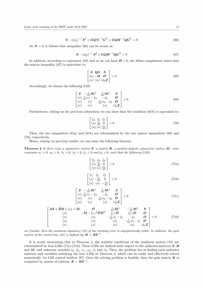
It is worth mentioning that in Theorem 2, the stability conditions of the nonlinear system (18) arereformulated by four LMIs (71a)-(71d). These LMIs are defined with respect to the unknown matrices S, Rand M , and unknown variables ξ1, ξ2, α1, α2, β1 and β2. Then, the problem lies in finding such unknownmatrices and variables satisfying the four LMIs in Theorem 2, which can be easily and effectively solvednumerically via LMI control toolbox [87]. Once the solving problem is feasible, then the gain matrix K iscomputed by means of relation: K = RS−1.

18 Gritli et al.

5 Simulation results of the limit cycle tracking

Simulation results are presented and discussed in the following. They attest to the effectiveness of the de-signed control law (20) for the tracking of the self-generated period-1 stable limit cycle using the gain matrixK, which is solution of LMIs in Theorem 2. We recall that the matrices A, B, D and C are given in thebeginning of Section 4. Moreover, σ = 10. Thus, by choosing ϵ = 0.1, the resolution of the four LMIs in (71)

by means of the LMI toolbox of MATLAB gives the following results: S =

49.5559 −16.3793 −10.6745−16.3793 20.9659 −20.6407−10.6745 −20.6407 50.1719

,M =

398.7800 −21.5710 −21.5706−21.5710 324.4302 −298.2469−21.5706 −298.2469 324.5022

,R =[1088.26 171.7705 −844.0613

], ξ1 = −570.8652, ξ2 = 886.3538,

α1 = α2 = 1497.858, and β1 = β2 = 1070.568. Therefore, the control gain K is computed to be: K =[48.5437 66.7622 20.9706

].

Table 2 shows some numerical values of the matrix gain K for some values of the parameter ϵ. Weemphasize that as ϵ decreases, the gain K increases. This increase in K will provoke a considerable increasein the control effort. However, the tracking error will be canceled rapidly as K increases. This will be shownnext.

Table 2 Numerical values of the gain matrix K for different values of ϵ.

ϵ K

0.1 [ 48.5437 66.7622 20.9706 ]0.05 [ 304.4274 603.7444 298.4429 ]0.01 [ 239.0992 500.4151 196.2109 ]0.005 [ 343.4758 786.0560 290.5334 ]0.001 [ 4768.16 10418.68 4837.79 ]0.0005 [ 3230.59 7633.10 2909.52 ]

We recall that K is the gain matrix of the stabilizing control law w defined by expression (22). Moreover,it is worth noting that the tracking control law (20) can be rewritten as:

v = Ke = K (x− xr) (72)

with K =[K (1) −k2 K (2) K (3)

], where K (i) is the ith element of the gain matrix K.

Furthermore, in order to avoid high gain of the tracking control law v in (72), we use a saturationfunction as follows:

v =

vmax if v > vmax

K (x− xr) if −vmax ≤ v ≤ vmax

−vmax if v < −vmax

(73)

where vmax = 10. Here, this value of vmax is an arbitrary choice.

We recall that xr is the state of the reference model (16), which generates the desired period-1 stablelimit cycle, whereas x is the state of the IWIP, as the physical system modeled via the nonlinear dynamics(15), under the tracking control law v (73).

Our objective is to investigate the influence of the designed control law v with the gain K on thedynamic behavior of the controlled IWIP and then the tracking of the self-generated period-1 stable limitcycle. Moreover, we will consider three different scenarios. The first scenario is the nominal case, for which thesystem is without parametric uncertainties and without external disturbing torque. In the second scenario,we will take into account uncertain parameters in the dynamics of the controlled IWIP. However, in thethird scenario, we will consider the external disturbance. We recall that the dynamics of the IWIP underparametric uncertainties in the friction coefficients δ1 and δ2 and subject to the external disturbing torqueζ is given by (17). The reference model generating the desired period-1 stable limit cycle is always thenominal one given by the dynamics (16). Moreover, in order to show how well behaved the closed-loopsystem is to the uncertainties in the two friction parameters δ1 and δ2 and the external disturbance ζ,we will realize several simulations. Indeed, we will consider and analyze different cases: constant uncertainfriction parameters, randomly time-varying uncertain parameters, a constant external disturbance, and arandomly time-varying external disturbance.


As noted previously, it was assumed that the physical device of the IWIP was mechanically designedin order to minimize the effects of viscous frictions [31, 34, 35, 53]. Thus, the frictions of the active andpassive joints are completely neglected. Authors in [44] calculated the viscous friction coefficient affectingthe actuator, the active joint. It was found to be about 10−4. In the next, we take a common value for thetwo friction parameters δ1 and δ2, δ1 = δ2 = 10−2.

5.1 First scenario: Nominal dynamics of the IWIP

In this first scenario, the IWIP is without uncertainties and external disturbances. As in [53], the proposedsimulation is started from the initial condition

(θ1(0), θ2(0), θ1(0), θ2(0)

)= (10, 0, 0 rad/s, 0 rad/s). The

choice of θ1(0) is motivated by the physical properties of the IWIP since simulation is started from the restposition at standstill. Moreover, we will take the gain matrix K computed for the parameter ϵ = 0.1 (seeTable 2).

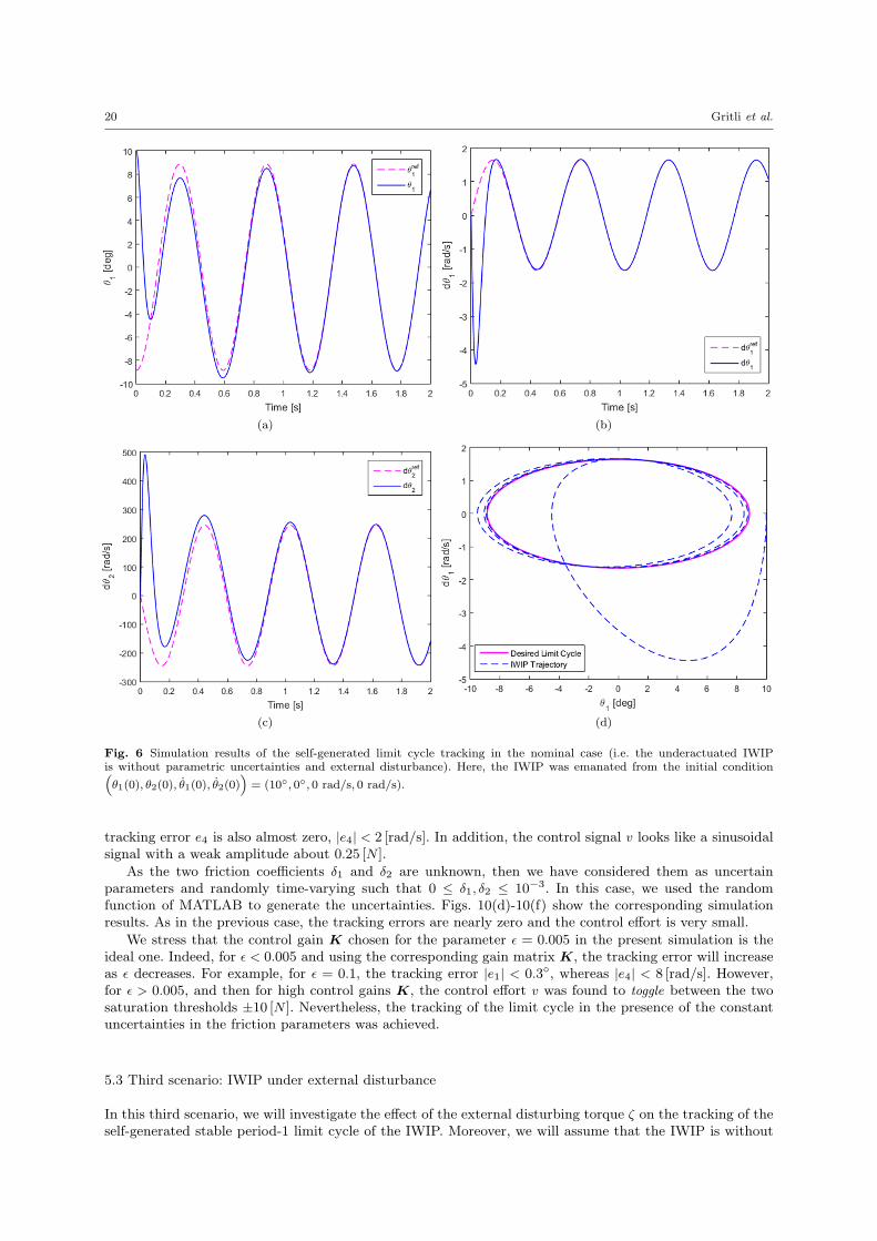
Then, application of the control law (73) to the nominal nonlinear dynamics (15) of IWIP gives theresults in Fig. 6. In each portrait of Fig. 6, we show the variable of the reference model and that of thecontrolled IWIP system, which is given by (15). Figure 6(a) shows the temporal evolution of the angularposition of the pendulum body, θ1. Figure 6(b) reveals the angular velocity of the pendulum θ1. Figure 6(c)depicts the angular velocity of the inertia wheel θ2. Figure 6(d) shows the desired period-1 stable limit cycleand the trajectory of the IWIP system under the control law (73) from the proposed initial condition. Theseresults show clearly the convergence of the trajectory of the controlled IWIP to the reference trajectoryand hence to the desired stable period-1 limit cycle. It can be observed from the displayed results that thetracking was achieved within almost three periods, since the period of the reference limit cycle is about0.6 [s]. Figure. 7 represents the tracking control law v. When the tracking was reached, the control law v

remains constant about the value −0.0614 [N ]. It is clear that the control effort is initially saturated at thevalue 10 [N ].

We have chosen another initial condition for the controlled IWIP such that θ1(0) is away from the track-ing trajectory. Then, using the same matrix gain K and the initial condition

(θ1(0), θ2(0), θ1(0), θ2(0)

)=

(0, 0, 0 rad/s, 0 rad/s), we obtained the simulation results in Fig. 8. Figure 8(a) shows the trajectory of thecontrolled IWIP in the state space with the desired period-1 stable limit cycle. Figure 8(b) shows temporalevolution of the tracking control law v.

In the two last simulation results, the initial condition was selected to respect the unilateral stateconstraints of the inverted pendulum given by (1). We have chosen other initial positions of the invertedpendulum such that the angular position θ1 is outside the interval [−σ σ]. In this case, the physical deviceof the underactuated IWIP is not that given in Fig. 1. The IWIP is not under the unilateral constraintsand its swing motion is completely free. In this case, we will have the inertial wheel pendulum studiedby Aguilar and his co-workers (see for example [45]) and other authors with different physical parameters.Figure 9 reveals simulation results of the underactuated IWIP for two initial positions of the invertedpendulum lying outside the defined working space (1). Figure 9(a) and Fig. 9(c) show the trajectory of theinverted pendulum in the state space and the corresponding self-generated limit cycle. However, Fig. 9(b)and Fig. 9(d) represent the tracking control law v. Figure 9(a) and Fig. 9(b) are plotted for the initialcondition θ1(0) = 90, whereas Fig. 9(c) and Fig. 9(d) are depicted for θ1(0) = 180. It is obvious that inthese two cases the trajectory of the IWIP follows the desired period-1 stable limit cycle. Moreover, thecontrol law v tends to a very small value (almost zero). It is worth noting that initially the control law v issaturated at ±10 [N ]. This is because the IWIP needs an important control effort to bring the IWIP fromits initial position to the desired one where the initial position was chosen to be far away from the trackingtrajectory.

5.2 Second scenario: IWIP under uncertain friction parameters

As noted before, in this second scenario, the two friction coefficients δ1 and δ2 of the passive and the activearticulations of the controlled underactuated IWIP are considered to be uncertain. Moreover, we will assumethat 0 ≤ δ1, δ2 ≤ 10−3. In this analysis, the initial condition of the IWIP is

(θ1(0), θ2(0), θ1(0), θ2(0)

)=

(10, 0, 0 rad/s, 0 rad/s). Furthermore, the gain matrix K is that calculated for the parameter ϵ = 0.005 inTable 2.

Figs. 10(a)-10(c) show simulation results for the case δ1 = δ2 = 10−3. In Fig. 10(a) and Fig. 10(b), weplotted the tracking errors e1 and e4, respectively. Figure 10(c) represents the signal of the control law v. Itis obvious that the tracking error e1 of the inverted pendulum is almost zero (|e1| < 0.04). Moreover, the

20 Gritli et al.

(a) (b)

(c) (d)

Fig. 6 Simulation results of the self-generated limit cycle tracking in the nominal case (i.e. the underactuated IWIPis without parametric uncertainties and external disturbance). Here, the IWIP was emanated from the initial condition(θ1(0), θ2(0), θ1(0), θ2(0)

)= (10, 0, 0 rad/s, 0 rad/s).

tracking error e4 is also almost zero, |e4| < 2 [rad/s]. In addition, the control signal v looks like a sinusoidalsignal with a weak amplitude about 0.25 [N ].

As the two friction coefficients δ1 and δ2 are unknown, then we have considered them as uncertainparameters and randomly time-varying such that 0 ≤ δ1, δ2 ≤ 10−3. In this case, we used the randomfunction of MATLAB to generate the uncertainties. Figs. 10(d)-10(f) show the corresponding simulationresults. As in the previous case, the tracking errors are nearly zero and the control effort is very small.

We stress that the control gain K chosen for the parameter ϵ = 0.005 in the present simulation is theideal one. Indeed, for ϵ < 0.005 and using the corresponding gain matrix K, the tracking error will increaseas ϵ decreases. For example, for ϵ = 0.1, the tracking error |e1| < 0.3, whereas |e4| < 8 [rad/s]. However,for ϵ > 0.005, and then for high control gains K, the control effort v was found to toggle between the twosaturation thresholds ±10 [N ]. Nevertheless, the tracking of the limit cycle in the presence of the constantuncertainties in the friction parameters was achieved.

5.3 Third scenario: IWIP under external disturbance

In this third scenario, we will investigate the effect of the external disturbing torque ζ on the tracking of theself-generated stable period-1 limit cycle of the IWIP. Moreover, we will assume that the IWIP is without


Fig. 7 Tracking control law v for the nominal dynamics of the underactuated IWIP for a first initial condition:(θ1(0), θ2(0), θ1(0), θ2(0)

)= (10, 0, 0 rad/s, 0 rad/s).

(a) (b)

Fig. 8 Simulation results of the self-generated limit cycle tracking in the nominal case for a new initial condition:(θ1(0), θ2(0), θ1(0), θ2(0)

)= (0, 0, 0 rad/s, 0 rad/s).

uncertainties, i.e. δ1 = δ2 = 0. We recall that the dynamics of the controlled IWIP under the disturbance ζ isgiven by (17). This disturbance is applied on the pendulum body. Furthermore, we assume that |ζ| ≤ ρ, withρ > 0. We will consider two cases: a constant disturbing torque ζ = ρ, and a randomly time-varying disturbingtorque ζ = ρ (2Rand− 1), with Rand is the function that generates random values between 0 and 1. In thisanalysis, the initial condition of the simulation is

(θ1(0), θ2(0), θ1(0), θ2(0)

)= (10, 0, 0 rad/s, 0 rad/s). In

addition, the disturbance ζ is applied during 3 [s] at the instant t = 2 [s]. Moreover, as in the previous study,the gain matrix K is chosen to be that calculated for the parameter ϵ = 0.005 in Table 2.

5.3.1 Case 1: Constant disturbance

In this first scenario, the value of the disturbing torque ζ applied to the controlled IWIP is constant: ζ = ρ.Figure 11 shows simulation results obtained for two different values of ρ. Figs. 11(a)-11(d) reveal the trackingunder the disturbance ζ = ρ = 0.5 [N ], whereas Fig. 11(e)-Fig. 11(h) depict the self-generated stable limitcycle tracking under the constant disturbance torque ζ = ρ = 1.5 [N ]. It is obvious that initially the desiredtrajectory (stable period-1 limit cycle) of the controlled IWIP was tracked. Once the disturbance ζ wasapplied on the IWIP, its behavior will be completely different. The motion of the pendulum and that of theinertia wheel diverge from the desired one. Moreover, it is worth noting that the angular position of the

22 Gritli et al.

(a) (b)

(c) (d)

Fig. 9 Self-generated limit cycle tracking of the underactuated IWIP in the nominal case for two initial conditions θ1(0)of the inverted pendulum lying outside the defined working state space (1). (a) and (b) for θ1(0) = 90. (c) and (d) forθ1(0) = 180.

inverted pendulum was found to not respect the unilateral constraints (1) (see Figs. 11(a) and 11(e)). Thisresult, although it is not real for the case of the physical device of the IWIP under study in this work, showsthat the proposed controller v was found to be able to bring the trajectory of the IWIP to the desired onedespite the presence of the constant disturbance ζ. Moreover, we emphasize that for ζ = ρ = 0.5 [N ], thecontrol law v converges to a constant value about −6 [N ] when the IWIP is under disturbance. However, ifζ = ρ = 1.5 [N ] then the control law was found to be saturated at −10 [N ]. Once the disturbance vanishes,the tracking was achieved again and the controller v becomes almost zero.

We stress that for ρ > 2 [N ] the motion of the controlled IWIP diverges completely from the desired one.The controller was found to be not able to bring the motion of the IWIP to the period-1 stable limit cyclewhen the disturbance was canceled.

5.3.2 Case 2: Randomly time-varying disturbance

In this second case, the external disturbing torque ζ varies randomly in time: ζ = ρ (2Rand− 1), with Randis the function that generates random values between 0 and 1. Thus, −ρ ≤ ζ ≤ ρ. Figure 12 reveal simulationresults for the controlled IWIP subject to the randomly time-varying external disturbing torque ζ. In thisanalysis, we have chosen ρ = 5. It is obvious that when the disturbance vanishes, the motion of the controlledIWIP returns to the period-1 stable oscillation. Moreover, the controller was found to compensate the effect


(a) (b) (c)

(d) (e) (f)

Fig. 10 Simulation results for the limit cycle tracking of the controlled IWIP for two different cases of frictions δ1 and δ2.In (a)-(c), δ1 = δ2 = 10−3. Whereas in (d)-(f), δ1 and δ2 are randomly time-varying. (a) and (d) show the tracking errore1 of the angular position of the inverted pendulum. (b) and (e) show the tracking error e4 of the angular velocity of theinertia wheel. (c) and (f) reveal the tracking control law v.

(a) (b) (c) (d)

(e) (f) (g) (h)

Fig. 11 Simulation results for the limit cycle tracking of the controlled IWIP under a constant disturbance torque ζ. In(a)-(d), ζ = ρ = 0.5 [N ], whereas in (e)-(h), ζ = ρ = 1.5 [N ]. (a) and (e) show the angular position of the inverted pendulum.(b) and (f) depict the angular velocity of the inverted pendulum. (c) and (g) represent the angular velocity of the inertiawheel. (d) and (h) reveal the tracking control law v.

of the external disturbing torque ζ. We stress that for ρ < 5, we have obtained almost the same resultsexcept the effect of the disturbance ζ decreases as ρ decreases.

We note that in Fig. 11 and Fig. 12, the motion area of pendulum (angular position θ1 in Fig. 11(a) andFig. 12(a)) is larger than 10. This fact contradicts with the motion constraint (1). In fact, in the numericalsimulation when the external disturbance ζ is applied, the condition (1) was not taken into account because

24 Gritli et al.

(a) (b) (c) (d)

Fig. 12 Simulation results for the limit cycle tracking of the controlled IWIP subject to a randomly time-varying externaldisturbing torque ζ. The maximal amplitude of such disturbance is ρ = 5. (a) shows the angular position of the invertedpendulum. (b) reveals the angular velocity of the inverted pendulum. (c) shows the angular velocity of the inertia wheel.(d) represents the control law v.

our main objective is to show the ability of the controlled IWIP to re-track the desired self-generated limitcycle even if it is subject to an external disturbance with a large amplitude under which the IWIP is veryfar from the desired one (as in Fig. 10 with an initial condition outside the required region). Thus, if we takethe state constraint (1) into consideration, then under the external disturbance, the pendulum will stuck(with some small oscillations) to the left/right mechanical stop until the disturbance is canceled or anotherexternal disturbance with small amplitude is applied. Hence, we will have θ1 = 10 for some stretches oftime.

Remark 6 It is worth pointing out that the choice of the external disturbing torque ζ to be randomly time-varying is arbitrary. It can be seen as a vibration signal applied to the IWIP. We can choose a regular form ofthe disturbing torque ζ, for example ζ(t) = Aζsin(wζt), where Aζ and wζ are respectively the amplitude andthe frequency of the disturbing torque ζ. Thus, we obtained almost the same results. When the disturbancewas canceled, the controlled IWIP returns to its self-generated stable limit cycle. Moreover, we can chooseanother regular form of the disturbing torque such as: ζ(t) = Aζe(−λζt). Here, the disturbing torque ζ willvanish progressively in time. We obtained also the same behavior of the controlled IWIP.

6 Conclusion and future works

In this paper, a control design approach is proposed for the tracking of a stable period-1 limit cycle ofan underactuated mechanical system: the inertia wheel inverted pendulum (IWIP). Such system is subjectto unilateral constraints limiting the swing motion of the pendulum body around its unstable equilibriumpoint. Moreover, an IDA-PBC was applied to the IWIP to control the underactuated IWIP at its uprightposition. By analyzing stability of the equilibrium point of the IWIP under the IDA-PBC and then existenceof the Hopf bifurcation, we showed that the controlled IWIP generated a stable limit cycle.

For some value of the gain parameter of the IDA-PBC, the nonlinear dynamics of the controlled IWIPwas adopted as the reference model generating the period-1 stable limit cycle, which is used as the track-ing trajectory for the IWIP. Thus, the tracking problem was transformed into a stabilization problem ofthe tracking error. We used first a predefined control law, which gave us a simplified model. Moreover, weadopted a state-feedback linear control law to asymptotically stabilize the tracking error. For this purpose,our methodology was based on the use of the second Lyapunov method and the S-procedure lemma. Thus,the stabilization problem was converted into a solving problem of BMIs. We employed the Schur comple-ment lemma and the matrix inversion lemma in order to transform such BMIs into LMIs. Finally, severalsimulations have been presented to corroborate the mathematical results and hence to show the feasibilityof the designed controller for the tracking of the self-generated limit cycle of the IWIP under the IDA-PBC.We analyzed three different scenarios: (1) a nominal dynamics of the IWIP, i.e. without uncertainties in pa-rameters and without disturbance, (2) IWIP under constant and randomly time-varying uncertain frictionparameters, and (3) IWIP subject to constant and randomly time-varying external disturbing torque appliedon the pendulum body. Simulation results showed that the control law was able, for some defined controlgain and a reasonable amplitude of the external disturbance, to compensate the effects of the uncertaintiesin the friction parameters and the external disturbance.

In this work, the control scheme is designed in the special case of the IWIP. However, our methodologyfor limit cycle tracking can be easily generalized to the more general case of underactuated mechanicalflat systems [12]. Moreover, as a future direction, we look for designing a robust tracking controller for the


IWIP with uncertain parameters and/or under external disturbances using the nonlinear dynamics (17).In addition, we look for designing an observer or an observer-based controller to control the IWIP to itsupright position or to track a desired trajectory.

Furthermore, we aim at verifying the obtained results in simulation via real-time experiments using theconstrained IWIP as in [34, 35, 53, 54] or that employed by [33].

Moreover, we showed that the control effort on the IWIP displayed oscillations if a constant frictionparameter is introduced. Thus, using the theory of the Hopf bifurcation as realized in this paper for thegeneration of periodic oscillations by varying the parameters of the IDA-PBC controller, we can demonstratetheoretically the birth of these oscillations by varying the friction parameter. This will be considered as ourmain future work.

In addition, we aim at extending our developed method of the state-feedback controller for the robusttracking of a desired limit cycle to more complex nonlinear systems. Our concern will be impulsive hybridnonlinear dynamics of biped robots studied by us in [88–90], and more particularly the passive dynamicwalking of the planar compass-gait biped robot [88] and the semi-passive dynamic walking of the torso-driven biped robot [89, 90]. Our design methodology of the tracking controller will be based on the LMItechniques.

Appendix 1: Self-generation of a limit cycle through Hopf bifurcation

In this Appendix, we show generation of a self-sustained oscillation (limit cycle) in the nonlinear dynamics ofthe underactuated IWIP under the IDA-PBC. Thus, we present first stability conditions of the equilibriumpoint xeq, given by expression (9), of the nonlinear dynamics (8). Moreover, we derive conditions provingexistence of the Hopf bifurcation and hence the periodic solutions in the nonlinear dynamics (8). Finally, wediscuss briefly stability of the periodic solutions using the fist Lyapunov value [4]. This quantity is calculatednumerically in this paper. Its mathematical description will be developed and presented in another newpaper. It is worth to note that analysis of 3D or 4D nonlinear dynamics has been widely investigated, as in[91–96], just to mention a few.

Appendix 1.1: Stability of the equilibrium point

We look for determining conditions on the control gains ki (i = 1, 2, 3, 4) for which the equilibrium point isstable and hence the Hopf bifurcation occurs.

For simplicity, posing a = 1I , b = bg and c = 1

I2. Then, the characteristic equation of the Jacobian matrix

(10) is defined as:

P (λ) = λ4 + (k3 − k4)λ3 + (a (γ − b+ k1)− ck2)λ

2 + abk4λ+ abck2 = 0 (74)

In order to study the stability conditions of the equilibrium point xeq, we apply Routh-Hurwitz criterion,which states that all real eigenvalues and all real parts of complex conjugate eigenvalues of the characteristicpolynomial P (λ) are negative if and only if the following conditions hold:

(i) a1 > 0, (ii) a3 > 0, (iii) a4 > 0 and (iv) a1a2a3 > a23 + a21a4 (75)

with ai (i = 1, 2, 3, 4), are defined such that:

P (λ) = λ4 + a1λ3 + a2λ

2 + a3λ+ a4 = 0 (76)

Applying Routh-Hurwitz criterion (75) to the characteristic polynomial (74), and as ki > 0 for i =1, 2, 3, 4, we find that necessary and sufficient conditions for the equilibrium point xeq to be asymptoticallystable are:

C1 = k3 − k4 > 0 (77a)

C2 = a (γ − b+ k1)− ck2 − abk4

k3 − k4− ck2

k3 − k4k4

> 0 (77b)

26 Gritli et al.

Appendix 1.2: Existence of Hopf bifurcation and periodic solutions

In this part, we will investigate existence of the Hopf bifurcation [4] at the equilibrium point regarding k4as the bifurcation parameter. Assume that (74) has a pure imaginary root λ = iw, w ∈ R+. Substituting itinto (74) yields

w4 − (a (γ − b+ k1)− ck2)w2 + abck2 + iw

(− (k3 − k4)w

2 + abk4

)= 0 (78)

It then follows that:

w4 − (a (γ − b+ k1)− ck2)w2 + abck2 = 0 (79a)

(k4 − k3)w2 + abk4 = 0 (79b)

From relation (79b), we obtain the following expression:

k4 =w2

ab+ w2k3 (80)

We stress that w is the solution of (79a) and it depends only on the two parameters k1 and k2. Moreover,according to expression (80), k4 is proportional to k3 and it depends on w. Then, by fixing the value of theparameters k1, k2 and k3, we can calculate the value of the gain k4 at which the Hopf bifurcation occurs.

By solving relation (79a), it is easy to show that there are two solutions wc1 and wc

2 defined as follows:

wc1 =

√√√√a (γ − b+ k1)− ck2 −√(a (γ − b+ k1)− ck2)

2 − 4abck2

2(81a)

wc2 =

√√√√a (γ − b+ k1)− ck2 +√(a (γ − b+ k1)− ck2)

2 − 4abck2

2(81b)

In (81), we have wc1 < wc

2. Actually, these two solutions, wc1 and wc

2, exist if and only if the followingthree conditions hold:

(a (γ − b+ k1)− ck2)2 − 4abck2 > 0 (82a)

a (γ − b+ k1)− ck2 −√(a (γ − b+ k1)− ck2)

2 − 4abck2 > 0 (82b)

a (γ − b+ k1)− ck2 +

√(a (γ − b+ k1)− ck2)

2 − 4abck2 > 0 (82c)

As k1 > 0 and k2 > 0, then according to conditions (82b) and (82c), it follows that: a (γ − b+ k1)−ck2 > 0.Therefore, relying on (82a), it easy to show that:

k1 > b− γ +c

ak2 + 2

√bc

a

√k2 (83)

This expression represents the condition on k1 with respect to k2 for the existence of the Hopf bifurcation.In addition, we emphasize that the system (8) exhibits two Hopf bifurcations at two different critical valueskc4,1 and kc4,2 that are associated to wc

1 and wc2, respectively. These two critical parameters kc4,1 and kc4,2 are

defined like so:

kc4,1 = k3a (γ − b+ k1)− ck2 −

√(a (γ − b+ k1)− ck2)

2 − 4abck2

a (γ + b+ k1)− ck2 −√(a (γ − b+ k1)− ck2)

2 − 4abck2

(84a)

kc4,2 = k3a (γ − b+ k1)− ck2 +

√(a (γ − b+ k1)− ck2)

2 − 4abck2

a (γ + b+ k1)− ck2 +√(a (γ − b+ k1)− ck2)

2 − 4abck2

(84b)

For example, for k1 = 1.036692, k2 = 0.0011 and k3 = 38.4, the two critical values of k4 at which theHopf bifurcation occurs are calculated to be about: kc4,1 = 0.87159917 and kc4,2 = 27.19772529. Moreover,we have: wc

1 = 1.04160466 and wc2 = 10.64970853.


It is worth noting that for k4 = kc4,i, (i = 1, 2), the relation C2 = 0 in (77b) takes place, for whichthe stability of the equilibrium is violated. Moreover, if the condition (83) is not satisfied, the two Hopfbifurcations disappear. In fact, there are two cases. The two Hopf bifurcations collide with each other andare replaced by only one Hopf bifurcation if the following condition is met:

k1 = b− γ +c

ak2 + 2

√bc

a

√k2 (85)

Hence, for such expression (90), we will obtain: wc1 = wc

2 = wc⋆ =

√√abc

√k2, and then:

kc4,⋆ = k3

√ck2√

ab+√ck2

(86)

Moreover, if k1 < b− γ + cak2 + 2

√bca

√k2, then no Hopf bifurcation exits.

Now, we aim at developing the analytical expression of the transversality condition for the occurrenceof the Hopf bifurcation. From (74), it follows that:

dλ (k4)

dk4=

iw(w2 + ab

)abk4 − 3 (k3 − k4)w2 + 2iw (a (γ − b+ k1)− ck2 − 2w2)

(87)

Thus, we obtain:

Re

(dλ (k4)

dk4

)=

2w2(w2 + ab

) (a (γ − b+ k1)− ck2 − 2w2

)(abk4 − 3 (k3 − k4)w2)2 + 4w2 (a (γ − b+ k1)− ck2 − 2w2)2

(88)

It is clear that the sign of the condition (88) depends on the quantity ϑ = a (γ − b+ k1) − ck2 − 2w2.

Using expressions of wc1 and wc

2, it follows that: ϑ =√(a (γ − b+ k1)− ck2)

2 − 4abck2 for w = wc1, and

ϑ = −√

(a (γ − b+ k1)− ck2)2 − 4abck2 for w = wc

2. Furthermore, based on condition (83), we obtain ϑ = 0

for the two cases. Therefore,

Re

(dλ (k4)

dk4

∣∣∣k4=kc4,i

,w=wci

)= 0 (89)

Accordingly, the second condition for the existence of a Hopf bifurcation [4] is also met. In addition, wehave:

Re

(dλ (k4)

dk4

∣∣∣k4=kc4,1,w=wc

1

)> 0 (90a)

Re

(dλ (k4)

dk4

∣∣∣k4=kc4,2,w=wc

2

)< 0 (90b)

Hence, according to condition (90a) the equilibrium point is stable when k4 > kc4,1 and periodic solutionsexist when k4 < kc4,1. Furthermore, according to condition (90b) the equilibrium point is stable whenk4 < kc4,2 and periodic solutions exist when k4 > kc4,2. Furthermore, the period Ti of oscillations around thebifurcation point kc4,i is defined as follows:

Ti =2π

wci

(91)

Appendix 1.3: Stability of the periodic solutions

In order to characterize the stability of the periodic solutions generated through each Hopf bifurcation, theso-called fist Lyapunov value (coefficient) [4], say ℓ1, must be computed and analyzed for the system (8).In the bifurcation points, a positive first Lyapunov value represents a subcritical bifurcation and predictsthat the system presents unstable periodic oscillations, which can fold back and coexist with the stableequilibrium point. In contrast, a negative value for ℓ1 indicates a supercritical bifurcation and stable self-oscillations emerge from the bifurcation point.

Analytical calculation of the fist Lyapunov coefficient ℓ1 can be achieved, but it is very long. It can becalculated according to the formula given in [97]. For the sake of brevity, we omit this calculation in thispaper. In fact, this analysis on stability of the periodic oscillations and bifurcation through the first Lyapunov

28 Gritli et al.

value and the center manifold theory will be developed with further details in another work. Then, in thisstudy we will perform a numerical computation of ℓ1 using the well-known MATCONT package [97, 98].Alonso et al. [57, 58] used the AUTO package to the numerical continuation of limit cycles and the stabilityindex for the underactuated IWP.

Thus, using MATCONT package, the fist Lyapunov coefficient ℓ1 is computed to be: ℓ1,1 = 3.121836×10−9 at kc4,1 = 0.87159917, whereas ℓ1,2 = −1.081602 × 10−5 at kc4,2 = 27.19772529. Therefore, as ℓ1,1 > 0then the periodic solution emanating from the first Hopf bifurcation at kc4,1 is unstable, and which arisesat the side where the equilibrium is stable. However, because ℓ1,2 < 0 hence the generated sustainedoscillation at the parameter kc4,2 is stable. Moreover, this stable periodic oscillation arises at the side wherethe equilibrium is unstable. Relying on relation (91), the period of the stable self-sustained oscillation (stablelimit cycle) around the critical parameter kc4,2 is: T2 = 0.5899866 [s].

Appendix 2: Equivalent BMI (29b) for a IWIP with uncertain friction parameters and an external

disturbance

Using the reference dynamics (16) and the uncertain disturbed nonlinear dynamics (17), we obtain thefollowing tracking error dynamics:

e = Je+D (f (x1)− f (xr1)) +Bv + Jx+ Dζ (92)

By substituting the tracking control law (20) in (92), system (92) will be simplified as follows:

˙e = Ae+ D (f (x1)− f (xr1)) + Bw + Ax+D5ζ (93)

with A =

0 0 0

0 − δ1+δ2I

δ2I2

0 δ2I − δ2

I2

and D5 =

010

.Moreover, the term Ax in (93) can be rewritten like so: Ax = δ1D2x3 + δ2D3x3 + δ2D4x4, with

D2 = 1I

0−10

, D3 = 1I

0−11

, D4 = 1I2

01−1

.In addition, if we consider that:

– the two uncertain friction parameters δ1 and δ2 are norm-bounded, i.e. δ1 ≤ δ1 and δ2 ≤ δ2,– the two states x3 and x4 are bounded such that |x3| < x3 and |x4| < x4, for some constants x3 > 0 and

x4 > 0,– the disturbance ζ is bounded such that |ζ| < ρ, with ρ > 0.

then, according to section 4.2 and relying on the Young relation, we obtain the following conditions:

2eTPAx ≤ eTP (M2 +M3 +M4)P e+(δ1x3

)2DT

2 M−12 D2 +

(δ2x3

)2DT

3 M−13 D3 +

(δ2x4

)2DT

4 M−14 D4

(94a)

2eTPD5ζ ≤ eTPM5P e+ ρ2DT5 M−1

5 D5 (94b)

with Mi = MTi > 0, i = 2, . . . , 5.

Let us pose J =

IIIII

, M = diag (M1,M2,M3,M4,M5), and D =

γD

δ1x3D2

δ2x3D3

δ2x4D4

ρD5

. Thus, based on results

in section 4.2, the BMI (29b) will be replaced by the following one:

[PA+ PBK + (⋆) + PJTMJP + η3I − (η1 − η2)C

(⋆) DTM−1D − ϵη3 + 4σ (η1 + η2)

]< 0 (95)


References

1. M. di Bernardo, K. H. Johansson, F. Vasca, Self-oscillations and sliding in relay feedback systems:Symmetry and bifurcations, International Journal of Bifurcation and Chaos 11 (04) (2001) 1121–1140.

2. A. Jenkins, Self-oscillation, Physics Reports 525 (2) (2013) 167–222.3. S. Chatterjee, Self-excited oscillation under nonlinear feedback with time-delay, Journal of Sound and

Vibration 330 (9) (2011) 1860–1876.4. J. Guckenheimer, P. Holmes, Nonlinear Oscillations, Dynamical Systems, and Bifurcations of Vector

Fields, 1st Edition, Applied Mathematical Sciences, Springer, New York, 1983.5. J. Sun, A. C. Luo, Bifurcation and Chaos in Complex Nonlinear Dynamical Systems, Advances in

Nonlinear Science and Complexity (Physics), Elsevier, 2006.6. S. H. Strogatz, Nonlinear Dynamics and Chaos: With Applications to Physics, Biology, Chemistry, and

Engineering, 2nd Edition, Studies in Nonlinearity, Westview Press, Colorado, 2014.7. K. T. Alligood, T. D. Sauer, J. A. Yorke, Chaos: An Introduction to Dynamical Systems, 1st Edition,

Textbooks in Mathematical Sciences, Springer, New York, 1996.8. A. Malas, S. Chatterjee, Generating self-excited oscillation in a class of mechanical systems by relay-

feedback, Nonlinear Dynamics 76 (2) (2014) 1253–1269.9. A. Malas, S. Chatterjee, Analysis and synthesis of modal and non-modal self-excited oscillations in a

class of mechanical systems with nonlinear velocity feedback, Journal of Sound and Vibration 334 (2015)296–318.

10. S. Wiggins, Introduction to Applied Nonlinear Dynamical Systems and Chaos, 2nd Edition, Vol. 2 ofTexts in Applied Mathematics, Springer, New York, 2003.

11. M. W. Spong, Underactuated mechanical systems, in: B. Siciliano, K. P. Valavanis (Eds.), ControlProblems in Robotics and Automation, Vol. 230 of Lecture Notes in Control and Information Sciences,Springer Berlin Heidelberg, 1998, pp. 135–150.

12. Y. Liu, H. Yu, A survey of underactuated mechanical systems, IET Control Theory Applications 7 (7)(2013) 921–935.

13. A. Choukchou-Braham, B. Cherki, M. Djemai, K. Busawon, Analysis and Control of UnderactuatedMechanical Systems, Springer-Verlag, New York, 2014.

14. A.-C. Huang, Y.-F. Chen, C.-Y. Kai, Adaptive Control of Underactuated Mechanical Systems, WorldScientific Publishing Co, Singapore, 2015.

15. I. Fantoni, R. Lozano, Nonlinear Control for Underactuated Mechanical Systems, Springer, London,2002.

16. S. Rudra, R. K. Barai, M. Maitra, Block Backstepping Design of Nonlinear State Feedback Control Lawfor Underactuated Mechanical Systems, 1st Edition, Springer, Singapore, 2017.

17. J. Moreno-Valenzuela, C. Aguilar-Avelar, S. Puga-Guzman, V. Santibanez, Two adaptive control strate-gies for trajectory tracking of the inertia wheel pendulum: neural networks vis a vis model regressor,Intelligent Automation & Soft Computing (2016) 1–11doi:10.1080/10798587.2015.1121618.

18. Z. Li, Y. Zhang, Robust adaptive motion/force control for wheeled inverted pendulums, Automatica46 (8) (2010) 1346–1353.

19. M. W. Spong, P. Corke, R. Lozano, Nonlinear control of the Reaction Wheel Pendulum, Automatica37 (2001) 1845–1851.

20. D. J. Block, K. J. Astrom, M. W. Spong, The Reaction Wheel Pendulum, 1st Edition, Synthesis Lectureson Control and Mechatronics, Morgan & Claypool, San Rafael, 2007.

21. R. Olfati-Saber, Nonlinear control of underactuated mechanical systems with application to roboticsand aerospace vehicles, Ph.D. thesis, Massachusetts Institute of Technology, Department ElectricalEngineering and Computer Science (2001).

22. R. Olfati-Saber, Global stabilization of a flat underactuated system : the inertia wheel pendulum, in:Proceedings of the CDC01-REG1152, 2001.

23. S. Ramamoorthy, B. Kuipers, Qualitative heterogeneous control of higher order systems, Hybrid Sys-tems: Computation and Control (2003) 417–434.

24. V. Santibanez, R. Kelly, J. Sandoval, Control of the inertia wheel pendulum by bounded torques, in:Proceedings of the European Control Conference and 44th IEEE Conference on Decision and Control,2005, pp. 8266–8270.

25. R. Ortega, M. Spong, F. Gomez-Estern, G. Blankenstein, Stabilization of a class of underactuatedmechanical systems via interconnection and damping assignment, IEEE Transactions on AutomaticControl 47 (8) (2002) 1218–1233.

30 Gritli et al.

26. R. Ortega, E. Garcia-Canseco, Interconnection and damping assignment passivity-based control: Asurvey, European Journal on control 10 (2004) 432–450.

27. R. Ortega, A. van der Schaft, B. Maschke, G. Escobar, Interconnection and damping assignmentpassivity-based control of port-controlled hamiltonian systems, Automatica 38 (4) (2002) 585–596.

28. F. Gomez-Estern, A. J. Van der Schaft, Physical damping in IDA-PBC controlled underactuated sys-tems, European Journal on control 10 (5) (2004) 451–468.

29. C. Aguilar-Ibanez, O. O. Gutierrez-Frias, M. S. Suarez-Castanon, Controlling the strongly dampinginertia wheel pendulum via nested saturation function, Computacion y Sistemas 12 (4) (2009) 436–449.

30. N. Qaiser, N. Iqbal, A. Hussain, N. Qaiser, Exponential stabilization of the inertia wheel pendulumusing dynamic surface control, Journal of Circuits, Systems and Computers 16 (01) (2007) 81–92.

31. N. Touati, A. Chemori, Predictive control for the stabilization of a fast mechatronic system : From sim-ulation to real-time experiments, in: Proceedings of the International IFAC Symposium on MechatronicSystems, 2013, pp. 237–242.

32. M. Olivares, P. Albertos, On the linear control of underactuated systems: The flywheel inverted pen-dulum, in: Proceedings of the 10th IEEE International Conference on Control and Automation, 2013,pp. 27–32.

33. M. Olivares, P. Albertos, Linear control of the flywheel inverted pendulum, ISA Transactions 53 (5)(2014) 1396–1403.

34. N. H. Khraief, A. Chemori, S. Belghith, External disturbance rejection in IDA-PBC controller forunderactuated mechanical systems: From theory to real time experiments, in: Proceedings of the IEEEConference on Control Applications, 2014, pp. 1747–1752.

35. N. H. Khraief, A. Chemori, J. J. Pena, S. Belghith, Stabilization of inertia wheel inverted pendulum bymodel reference adaptive IDA-PBC: From simulation to real-time experiments, in: Proceedings of the3rd International Conference onControl, Engineering Information Technology (CEIT), 2015, pp. 1–6.

36. M. Ryalat, D. S. Laila, A simplified IDA-PBC design for underactuated mechanical systems with ap-plications, European Journal of Control 27 (2016) 1–16.

37. Z.-Q. Guo, J.-X. Xu, T. H. Lee, Design and implementation of a new sliding mode controller on anunderactuated wheeled inverted pendulum, Journal of the Franklin Institute 351 (2014) 2261–2282.

38. S. Mobayen, Design of LMI-based sliding mode controller with an exponential policy for a class ofunderactuated systems, Complexity (2014) 1–8.

39. M. Yue, X. Sun, N. Li, C. An, Dynamic motion planning and adaptive tracking control for a classof two-wheeled autonomous vehicle with an underactuated pendular suspension, Journal of DynamicSystems, Measurement, and Control 137 (10) (2015) DS–15–1019.

40. A. Zhang, C. Yang, S. Gong, J. Qiu, Nonlinear stabilizing control of underactuated inertia wheel pen-dulum based on coordinate transformation and time-reverse strategy, Nonlinear Dynamics 84 (4) (2016)2467–2476.

41. L. T. Aguilar, I. Boiko, L. Fridman, R. Iriarte, Generating self-excited oscillations via two-relay con-troller, IEEE Transaction on Automatic Control 54 (2) (2009) 416–420.

42. L. T. Aguilar, I. Boiko, L. Fridman, R. Iriarte, Generating self-excited oscillations for underactuatedmechanical systems via two-relay controller, International Journal of Control 82 (9) (2009) 1678–1691.

43. L. T. Aguilar, I. Boiko, L. Fridman, L. Freidovich, Generating oscillations in inertia wheel pendulumvia two relay controller, International Journal of Robust and Nonlinear Control 22 (2012) 318–330.

44. R. Iriarte, L. T. Aguilar, L. Fridman, Second order sliding mode tracking controller for inertia wheelpendulum, Journal of the Franklin Institute 350 (2013) 92–106.

45. L. T. Aguilar, I. Boiko, L. Fridman, R. Iriarte, Self-Oscillations in Dynamic Systems: A New Methodol-ogy via Two-Relay Controllers, 1st Edition, Birkhauser Basel, Springer International Publishing Switzer-land, 2015.

46. A. Estrada, L. T. Aguilar, R. Iriarte, L. Fridman, Two relay controller for real time trajectory generationand its application to inverted orbital stabilization of inertia wheel pendulum via quasi-continuousHOSM, Asian Journal of Control 14 (1) (2012) 58–66.

47. L. B. Freidovich, P. X. L. Hera, U. Mettin, A. Robertsson, A. S. Shiriaev, R. Johansson, Shaping stableperiodic motions of inertia wheel pendulum: Theory and experiment, Asian Journal of Control 11 (5).

48. A. S. Shiriaev, J. W. Perram, C. C. de Wit, Constructive tool for orbital stabilization of underactuatednonlinear systems: Virtual constraints approach, IEEE Transaction on Automatic Control 50 (2005)1164–1176.

49. A. Shiriaev, J. Perram, A. Robertsson, A. Sandberg, Periodic motion planning for virtually constrainedEuler-Lagrange systems, Systems and Control Letters 55 (2006) 900–907.


50. A. S. Shiriaev, L. B. Freidovich, I. R. Manchester, Can we make a robot ballerina perform a pirou-ette? orbital stabilization of periodic motions of underactuated mechanical systems, Annual Reviews inControl 32 (2) (2008) 200–211.

51. C. Gruber, M. Hofbaur, Periodic Motion Control of the Reaction Wheel Pendulum, in: 13th MechatronicForum, 2012, pp. 1–8.

52. S. Andary, A. Chemori, S. Krut, Stable Limit Cycle Generation for Underactuated Mechanical Sys-tems, Application: Inertia Wheel Inverted Pendulum, in: Proceedings of the IEEE/RSJ InternationalConference on Intelligent RObots and Systems, 2008, pp. 526–531.

53. S. Andary, A. Chemori, S. Krut, Control of the underactuated inertia wheel inverted pendulum forstable limit cycle generation, Advanced Robotics 23 (15) (2009) 1999–2014.

54. S. Andary, A. Chemori, S. Krut, Estimation-based disturbance rejection in control for limit cycle gen-eration on inertia wheel inverted pendulum testbed, in: Proceedings of the IEEE/RSJ InternationalConference on Intelligent RObots and Systems, 2009, pp. 1302–1307.

55. C. Zayane-Aissa, T.-M. Laleg-Kirati, A. Chemori, Control of a perturbed under-actuated mechanicalsystem, in: Proceedings of the IEEE Multi-Conference on Systems and Control, 2015, pp. 294–299.

56. C. A.-I. anez, J. C. Martinez, J. de Jesus Rubio, M. S. Suarez-Castanon, Inducing sustained oscillationsin feedback-linearizable single-input nonlinear systems, ISA Transactions 54 (2015) 117–124.

57. D. M. Alonso, E. E. Paolini, J. L. Moiola, Global bifurcation analysis of a controlled underactuatedmechanical system, Nonlinear Dynamics 40 (3) (2005) 205–225.

58. D. M. Alonso, E. E. Paolini, J. L. Moiola, Controlling an inverted pendulum with bounded controls,in: F. Colonius, L. Grune (Eds.), Dynamics, Bifurcations, and Control, Vol. 273 of Lecture Notes inControl and Information Sciences, Springer Berlin Heidelberg, 2002, pp. 3–16.

59. D. Pagano, L. Pizarro, J. Aracil, Local bifurcation analysis in the Furuta pendulum via normal forms,International Journal of Bifurcation and Chaos 10 (5) (2000) 981–995.

60. S. Nikolov, V. Nedev, Bifurcation analysis and dynamic behaviour of an inverted pendulum withbounded control, Journal of Theoretical and Applied Mechanics 64 (1) (2016) 17–32.

61. S. Boyd, L. El-Ghaoui, E. Feron, V. Balakrishnan, Linear matrix inequalities in system and controltheory, 1st Edition, Vol. 15 of Studies in Applied and Numerical Mathematics, SIAM, Philadelphia,PA., 1994.

62. I. R. Petersen, R. Tempo, Robust control of uncertain systems: Classical results and recent developments,Automatica 50 (5) (2014) 1315–1335.

63. R. C. L. F. Oliveira, M. C. de Oliveira, P. L. D. Peres, Robust state feedback LMI methods forcontinuous-time linear systems: Discussions, extensions and numerical comparisons, in: 2011 IEEE In-ternational Symposium on Computer-Aided Control System Design (CACSD), 2011, pp. 1038–1043.

64. L. A. Rodrigues, R. C. L. F. Oliveira, J. F. Camino, New extended LMI characterization for state feed-back control of continuous-time uncertain linear systems, in: Control Conference (ECC), 2015 European,2015, pp. 1992–1997.

65. F. Pfeiffer, C. Glocker, Multibody Dynamics with Unilateral Contacts, Wiley Series in Nonlinear Science,Wiley-VCH Verlag GmbH & Co. KGaA, Weinheim, 2004.

66. A.-C. Huang, Y.-C. Chen, Adaptive sliding control for single-link flexible-joint robot with mismatcheduncertainties, IEEE Transactions on Control Systems Technology 12 (5) (2004) 770–775.

67. M. Hosseinpour, P. Nikdel, M. Badamchizadeh, M. Akbari, Modelling and control of flexible joint robotbased on Takagi-Sugeno fuzzy approach and its stability analysis via sum of squares, Mathematical andComputer Modelling of Dynamical Systems 19 (3) (2013) 250–262.

68. K. Merat, H. Salarieh, A. Alasty, A. Meghdari, Stochastic piecewise affine control with application topitch control of helicopter, Nonlinear Analysis: Hybrid Systems 15 (2015) 86–97.

69. H. Razavi, K. Merat, H. Salarieh, A. Alasty, A. Meghdari, Observer based minimum variance controlof uncertain piecewise affine systems subject to additive noise, Nonlinear Analysis: Hybrid Systems 19(2016) 153–167.

70. R. C. Luo, J. Sheng, C. C. Chen, P. H. Chang, C. I. Lin, Biped robot push and recovery using fly-wheel model based walking perturbation counteraction, in: 13th IEEE-RAS International Conferenceon Humanoid Robots (Humanoids), 2013, pp. 50–55.

71. R. C. Luo, C. W. Huang, A push-recovery method for walking biped robot based on 3-D flywheelmodel, in: 41st Annual Conference of the IEEE Industrial Electronics Society, IECON 2015, 2015, pp.2685–2690.

72. M. Shafiee-Ashtiani, A. Yousefi-Koma, M. S. Panahi, M. Khadiv, Push recovery of a humanoid robotbased on model predictive control and capture point, CoRR abs/1612.08034.URL http://arxiv.org/abs/1612.08034

32 Gritli et al.

73. J. Pratt, J. Carff, S. Drakunov, A. Goswami, Capture point: A step toward humanoid push recovery,in: 2006 6th IEEE-RAS International Conference on Humanoid Robots, 2006, pp. 200–207.

74. E. R. Westervelt, J. W. Grizzle, C. Chevallereau, J.-H. Choi, B. Morris, Feedback control of dynamicbipedal robot locomotion, Taylor & Francis/CRC, London, 2007.

75. C. E. de Brito Novaes, P. S. P. da Silva, P. Rouchon, Trajectory control of a bipedal walking robot withinertial disc, IFAC Proceedings Volumes 47 (3) (2014) 4843–4848, 19th IFAC World Congress.

76. C. E. de Brito Novaes, P. S. P. da Silva, Numerical estimation of stability region of self-clocked bipedalrobots with inertial disk, Journal of Control, Automation and Electrical Systems 27 (6) (2016) 634–645.

77. B. M. Fard, A. Bagheri, N. Nariman-Zadeh, Limit cycle walker push recovery based on a receding horizoncontrol scheme, Proceedings of the Institution of Mechanical Engineers, Part I: Journal of Systems andControl Engineering 226 (7) (2012) 914–926.

78. Y. Zhu, Y. Gao, C. Xu, J. Zhao, H. Jin, J. Lee, Adaptive control of a gyroscopically stabilized pendulumand its application to a single-wheel pendulum robot, IEEE/ASME Transactions on Mechatronics 20 (5)(2015) 2095–2106.

79. M. W. Spong, M. Vidyasagar, Robot Dynamics and Control, 1st Edition, John Wiley & Sons, NewYork, NY, USA, 1989.

80. T. S. Parker, L. O. Chua, Practical numerical algorithms for chaotic systems, Springer, New York, 1989.81. C. Scherer, S. Weiland, Linear Matrix Inequalities in Control, Dutch Institute of Systems and Control

(DISC), The Netherlands, 2005.82. M. M. Asheghan, M. T. Beheshti, An LMI approach to robust synchronization of a class of chaotic

systems with gain variations, Chaos, Solitons & Fractals 42 (2) (2009) 1106–1111.83. S. Mobayen, An LMI-based robust controller design using global nonlinear sliding surfaces and appli-

cation to chaotic systems, Nonlinear Dynamics 79 (2) (2015) 1075–1084.84. T. Kailath, Linear Systems, Prentice-Hall, Englewood Cliffs, NJ,, 1989.85. N. J. Higham, Accuracy and Stability of Numerical Algorithms, 2nd Edition, Society for Industrial and

Applied Mathematics, Philadelphia, PA, USA, 2002.86. J. G. VanAntwerp, R. D. Braatz, A tutorial on linear and bilinear matrix inequalities, Journal of Process

Control 10 (4) (2000) 363–385.87. P. Gahinet, A. Nemirovski, A. J. Laub, M. Chilali, LMI control toolbox. For Use with MATLAB,

MathWorks, Natick, Massachusetts, 1995.88. H. Gritli, S. Belghith, Walking dynamics of the passive compass-gait model under OGY-based control:

Emergence of bifurcations and chaos, Communications in Nonlinear Science and Numerical Simulation47 (2017) 308–327.

89. H. Gritli, S. Belghith, N. Khraeif, OGY-based control of chaos in semi-passive dynamic walking of atorso-driven biped robot, Nonlinear Dynamics 79 (2) (2015) 1363–1384.

90. H. Gritli, S. Belghith, Bifurcations and chaos in the semi-passive bipedal dynamic walking model undera modified OGY-based control approach, Nonlinear Dynamics 83 (4) (2016) 1955–1973.

91. Z. Wang, L. Zhou, Z. Chen, J. Wang, Local bifurcation analysis and topological horseshoe of a 4Dhyper-chaotic system, Nonlinear Dynamics 83 (4) (2016) 2055–2066.

92. L. Zhou, Z. Chen, Z. Wang, J. Wang, On the analysis of local bifurcation and topological horseshoe ofa new 4D hyper-chaotic system, Chaos, Solitons & Fractals 91 (2016) 148–156.

93. W. Wu, Z. Chen, Hopf bifurcation and intermittent transition to hyperchaos inA aA novel strongfour-dimensional hyperchaotic system, Nonlinear Dynamics 60 (4) (2010) 615–630.

94. X. Li, P. Wang, Hopf bifurcation and heteroclinic orbit in a 3D autonomous chaotic system, NonlinearDynamics 73 (1) (2013) 621–632.

95. A. Algaba, M. C. Domınguez-Moreno, M. Merino, A. J. Rodrıguez-Luis, Study of the Hopf bifurcationin the Lorenz, Chen and Lu systems, Nonlinear Dynamics 79 (2) (2015) 885–902.

96. K. Deng, S. Yu, Hopf bifurcation analysis of a new modified hyperchaotic Lu system, Optik - Interna-tional Journal for Light and Electron Optics 124 (23) (2013) 6265–6269.

97. W. Govaerts, Numerical bifurcation analysis for ODEs, Journal of Computational and Applied Mathe-matics 125 (1–2) (2000) 57–68.

98. A. Dhooge, W. Govaerts, Y. A. Kuznetsov, MATCONT: A MATLAB package for numerical bifurcationanalysis of ODEs, ACM Transactions on Mathematical Software 29 (2) (2003) 141–164.

Documents

Self-generated limit cycle tracking of the underactuated