INVERSIONOF MAGNETIC ANOMALIES DUE TO 2-D CYLINDRICAL

International Journal on Soft Computing (IJSC) Vol.10, No.1, February 2019

DOI: 10.5121/ijsc.2019.10101 1

INVERSIONOF MAGNETIC ANOMALIES DUE TO 2-D CYLINDRICAL STRUCTURES –BY

AN ARTIFICIAL NEURAL NETWORK

Bhagwan Das Mamidala1 and Sundararajan Narasimman2

1Department of Mathematics, Osmania University, Hyderabad-500 007, India 2Department of Earth Science, Sultan Qaboos University, Muscat, Oman

ABSTRACT

Application of Artificial Neural Network Committee Machine (ANNCM) for the inversion of magnetic

anomalies caused by a long-2D horizontal circular cylinder is presented. Although, the subsurface targets

are of arbitrary shape, they are assumed to be regular geometrical shape for convenience of mathematical

analysis. ANNCM inversion extract the parameters of the causative subsurface targets include depth to the

centre of the cylinder (Z), the inclination of magnetic vector(Ɵ)and the constant term (A)comprising the radius(R)and the intensity of the magnetic field(I). The method of inversion is demonstrated over a

theoretical model with and without random noise in order to study the effect of noise on the technique and

then extended to real field data. It is noted that the method under discussion ensures fairly accurate results

even in the presence of noise. ANNCM analysis of vertical magnetic anomaly near Karimnagar, Telangana,

India, has shown satisfactory results in comparison with other inversion techniques that are in vogue.The

statistics of the predicted parameters relative to the measured data, show lower sum error (<9.58%) and

higher correlation coefficient (R>91%) indicating that good matching and correlation is achieved between

the measured and predicted parameters.

KEYWORDS

Magnetic anomaly, Artificial Neural Network, Committee machine, Levenberg – Marquardt algorithm,

Hilbert transform, modified Hilbert transform, trial and error method.

1. INTRODUCTION

In quantitative interpretation, the gravity and magnetic anomalies over a mineralized zone or

geological structure can be approximated to simple geometrical shapes. Quantitativeinterpretation of the magnetic and gravity anomalies due to anticlines and synclines is accomplished by

approximating them to two-dimensional, long horizontal circular cylinder. Linear concentrations

of the mineral magnetite in a mineralized zone may be approximated some times to a horizontal cylinder. There are several methods of analyzing magnetic anomalies due to cylindrical

structure.Parker Gay(1965) presented a set of master curves for the interpretation of the magnetic

anomalies due to cylindrical bodies [25]. Rao et al. (1973) have developed direct methods for

carrying out such interpretations [28]. Murthyand Mishra (1980) have proposed spectral approaches[23].

Mohan et al. (1990) used the Mellin transform in interpreting magnetic anomalies due to some

two dimensional bodies [21].Sundararajan et al. (1985, 1989) interpreted the magnetic anomalies of various components due to thin infinite dyke and spherical source by using Hilbert

transform([34], [35]). Srinivas(1998) used the modified Hilbert transform to interpret magnetic

anomalies caused by 2-D horizontal circular cylindrical structures [32].During 1999-2013, different methods Wavelet transform([22], [16]), Displacement of the maximum and minimum by


2

upward continuation [9], Euler deconvolution [12], Fraser filter [5], Hartley transform [18] and

Direct analytic signal [6] were used for inversion of magnetic data.

TDX is a normalized version of the horizontal derivative filter and can recognize the edges of the shallow and deep bodies simultaneously. This filter is commonly used in the edge detection of

potential field data.Alamdar et al. (2015) used combination of this balanced edge detection filter

and Euler deconvolution to real magnetic data from Soork iron ore mine in Iran to estimate source

location [1].Tavakoli et al. (2016) used singular value decomposition method for the interpretation of magnetic anomalies by 3D inversion [38]. Very fast simulated annealing global

optimization technique is used for interpretation of gravity and magnetic anomaly over thin sheet-

type structure byArkoprovo Biswas (2016) [3]. Recently, YunusLeventEkinci et al. (2017) used differential evolution algorithm for amplitude inversion of the 2D analytic signal of magnetic

anomalies [39].In the recent years, soft computing tools like Artificial neural network (ANN),

Fuzzy logic, Genetic algorithm gained great importance in geophysical data inversion([17], [33],

[30], [14], [10], [26], [2]).

A committee machine consists of a group of intelligent systems named experts (ANN) and a

combiner which combines the outputs of each expert[8].Its advantages aremore accuracy in

prediction,speed learningand better generalization.If the combination of experts in committee machine were replaced by a single neural network, one would have a network with a

correspondingly large number of adjustable weight parameters. The training time for such a large

network is likely to be longer than for the case of a set of experts trained in parallel. Moreover, the risk of over fitting the data increases when the number of adjustable weight parameters is

large compared to size of the set of the training data.

In this paper, the analysis of vertical magnetic anomalies due to a 2-D horizontal circular cylinder is carried out using ANN-based committee machine.The method is illustrated with the study of

theoretical model and validity of procedure is tested with the addition of random noise to the

source data. Further, the technique is exemplified with magneticanomaly over a narrow band of quartz magnetic nearKarimnagar, Telangana, India [32]. Both the theoretical as well as field data

yield reasonably good resultsand are compared with other methods that are in vogue.

2. ARTIFICIAL NEURAL NETWORKS

An artificial neural network is a computing system which consists of massively parallel

interconnection of large number of neurons. It is capable of capturing and representing complex input/output relationships and is an abstract simulation of a human brain. It learns incrementally

from environment (data). On this basis it provides reliable predictions for new situations

containing even noisy and partial information. ANN has two main components, namely the processing elements and the connections between them. The processing elements are called

neurons and connection between two neurons is called a link. Every link has a weight parameter

associated with it. A neuron ( j ) computes a single output ( )ja from multiple inputs

01 2( , , ... , )Sx x x by forming linear combination according to its input weights

01 2( , , ... .. ., , )j j jS jw w w b and then possibly putting the output through some activation function (

(.)f ) and is shown in Figure (1)([20], [29], [8]), where 0S is the number of inputs. Activation

functions such as sigmoid are commonly used since they are nonlinear and continuously

differentiable([11], [31]).The neurons take input data and perform simple operations on the data.

The result of these operations is passed to other neurons. ANNs are capable of learning, which takes place by altering weight values.


3

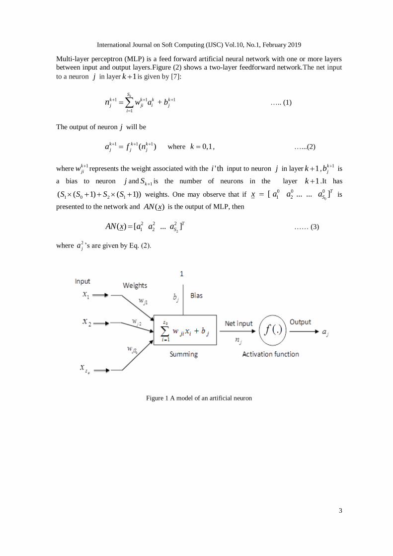
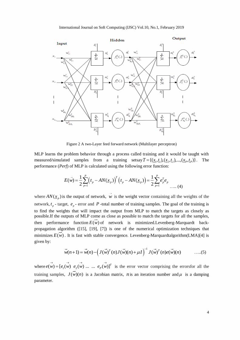
Multi-layer perceptron (MLP) is a feed forward artificial neural network with one or more layers

between input and output layers.Figure (2) shows a two-layer feedforward network.The net input

to a neuron j in layer 1k is given by [7]:

1 1 1

1

+ kS

k k k k

j ji i j

i

w a bn

….. (1)

The output of neuron j will be

1 1 1( ) k k k

j j ja f n where 0,1k , …...(2)

where1k

jiw represents the weight associated with the ' thi input to neuron j in layer 1k ,

1k

jb is

a bias to neuron j and1kS is the number of neurons in the layer 1k .It has

1 0 2 1( ( 1) ( 1))S S S S weights. One may observe that if 0

0 0 0

1 2 [ ... ... ]T

Sx a a a is

presented to the network and ( )AN x is the output of MLP, then

2

2 2 2

1 2( ) [ ... ]T

SAN x a a a

…… (3)

where 2

ja ’s are given by Eq. (2).

Figure 1 A model of an artificial neuron


4

Figure 2 A two-Layer feed forward network (Multilayer perceptron) MLP learns the problem behavior through a process called training and it would be taught with

measured/simulated samples from a training setsay 1 1 2 2{( , ),( , ),...,( , )}P PT x t x t x t . The

performance (Perf) of MLP is calculated using the following error function:

1 1

1 1( ) ( ) ( )

2 2

P PT

T

p pp p p p

p p

E w t AN x t AN x e e

….. (4)

where ( )pAN x is the output of network, w is the weight vector containing all the weights of the

network, pt - target, pe - error and P -total number of training samples. The goal of the training is

to find the weights that will impact the output from MLP to match the targets as closely as

possible.If the outputs of MLP come as close as possible to match the targets for all the samples,

then performance function ( )E w of network is minimized.Levenberg-Marquardt back-

propagation algorithm ([15], [19], [7]) is one of the numerical optimization techniques that

minimizes ( )E w . It is fast with stable convergence. Levenberg-Marquardtalgorithm(LMA)[4] is

given by:

1

( 1) ( ) ( ) ( ) ( )( ) ( ) ( ) ( )( )T Tw n w n J w n J w n I J w n e w n

…..(5)

where 1 2( ) [ ( ) ( ) ... ... ( )]T

Pe w e w e w e w

is the error vector comprising the errorsfor all the

training samples, ( )( )J w n is a Jacobian matrix, n is an iteration number and is a damping

parameter.


5

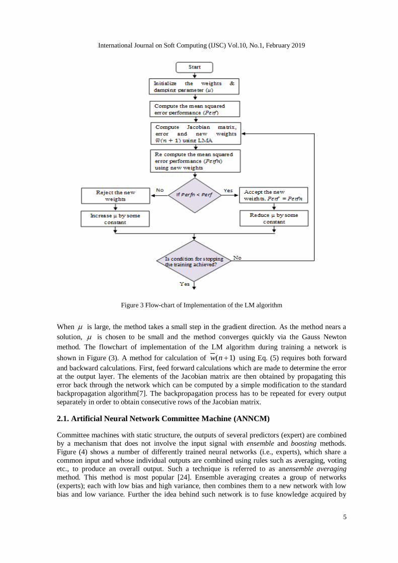
Figure 3 Flow-chart of Implementation of the LM algorithm

When is large, the method takes a small step in the gradient direction. As the method nears a

solution, is chosen to be small and the method converges quickly via the Gauss Newton

method. The flowchart of implementation of the LM algorithm during training a network is

shown in Figure (3). A method for calculation of ( 1)w n using Eq. (5) requires both forward

and backward calculations. First, feed forward calculations which are made to determine the error at the output layer. The elements of the Jacobian matrix are then obtained by propagating this

error back through the network which can be computed by a simple modification to the standard

backpropagation algorithm[7]. The backpropagation process has to be repeated for every output

separately in order to obtain consecutive rows of the Jacobian matrix.

2.1. Artificial Neural Network Committee Machine (ANNCM)

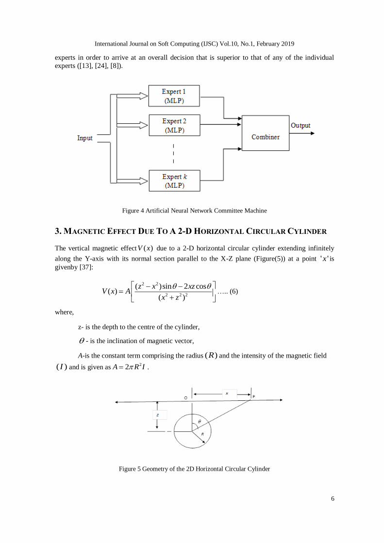
Committee machines with static structure, the outputs of several predictors (expert) are combined by a mechanism that does not involve the input signal with ensemble and boosting methods.

Figure (4) shows a number of differently trained neural networks (i.e., experts), which share a

common input and whose individual outputs are combined using rules such as averaging, voting etc., to produce an overall output. Such a technique is referred to as anensemble averaging

method. This method is most popular [24]. Ensemble averaging creates a group of networks

(experts); each with low bias and high variance, then combines them to a new network with low

bias and low variance. Further the idea behind such network is to fuse knowledge acquired by


6

experts in order to arrive at an overall decision that is superior to that of any of the individual

experts ([13], [24], [8]).

Figure 4 Artificial Neural Network Committee Machine

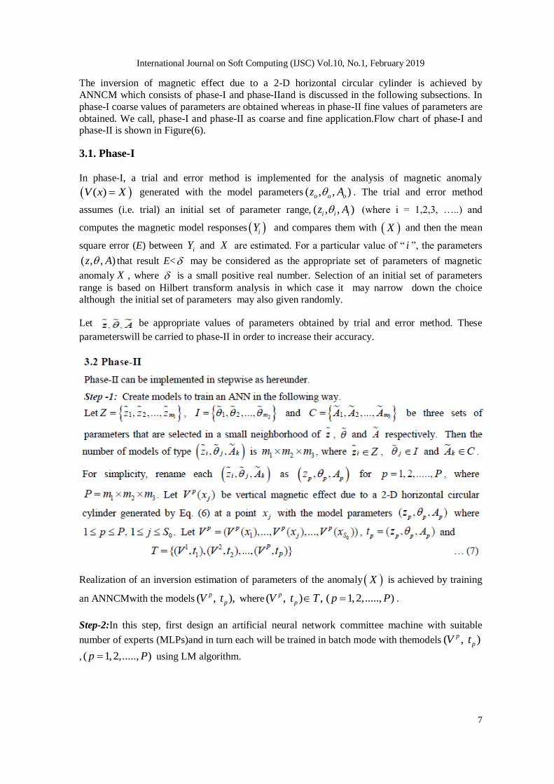
3. MAGNETIC EFFECT DUE TO A 2-D HORIZONTAL CIRCULAR CYLINDER

The vertical magnetic effect ( )V x due to a 2-D horizontal circular cylinder extending infinitely

along the Y-axis with its normal section parallel to the X-Z plane (Figure(5)) at a point ' 'x is

givenby [37]:

2 2

2 2 2

( )sin 2 cos( )

( )

z x xzV x A

x z

….. (6)

where,

z- is the depth to the centre of the cylinder,

- is the inclination of magnetic vector,

A-is the constant term comprising the radius ( )R and the intensity of the magnetic field

( )I and is given as22A R I .

Figure 5 Geometry of the 2D Horizontal Circular Cylinder


7

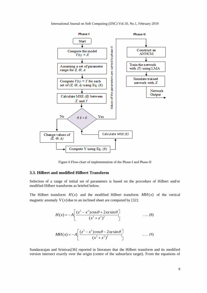
The inversion of magnetic effect due to a 2-D horizontal circular cylinder is achieved by

ANNCM which consists of phase-I and phase-IIand is discussed in the following subsections. In

phase-I coarse values of parameters are obtained whereas in phase-II fine values of parameters are

obtained. We call, phase-I and phase-II as coarse and fine application.Flow chart of phase-I and phase-II is shown in Figure(6).

3.1. Phase-I

In phase-I, a trial and error method is implemented for the analysis of magnetic anomaly

( )V x X generated with the model parameters ( , , )o o oz A . The trial and error method

assumes (i.e. trial) an initial set of parameter range, ( , , )i i iz A (where i = 1,2,3, …..) and

computes the magnetic model responses iY and compares them with X and then the mean

square error (E) between iY and X are estimated. For a particular value of “ i ”, the parameters

( , , )z A that result E< may be considered as the appropriate set of parameters of magnetic

anomaly X , where is a small positive real number. Selection of an initial set of parameters

range is based on Hilbert transform analysis in which case it may narrow down the choice

although the initial set of parameters may also given randomly.

Let be appropriate values of parameters obtained by trial and error method. These

parameterswill be carried to phase-II in order to increase their accuracy.

Realization of an inversion estimation of parameters of the anomaly X is achieved by training

an ANNCMwith the models ( , ),p

pV t where ( , ) ,p

pV t T ( 1,2,....., )p P .

Step-2:In this step, first design an artificial neural network committee machine with suitable

number of experts (MLPs)and in turn each will be trained in batch mode with themodels ( , )p

pV t

, ( 1,2,....., )p P using LM algorithm.


8

Figure 6 Flow-chart of implementation of the Phase-I and Phase-II

3.3. Hilbert and modified Hilbert Transform

Selection of a range of initial set of parameters is based on the procedure of Hilbert and/or

modified Hilbert transforms as briefed below.

The Hilbert transform ( )H x and the modified Hilbert transform ( )MH x of the vertical

magnetic anomaly ( )V x due to an inclined sheet are computed by [32]:

2 2

2 2 2

( )cos 2 sin( )

( )

z x xzH x A

x z

….. (8)

2 2

2 2 2

( )cos 2 sin( )

( )

z x xzMH x A

x z

..… (9)

Sundararajan and Srinivas[36] reported in literature that the Hilbert transform and its modified version intersect exactly over the origin (centre of the subsurface target). From the equations of


9

vertical magnetic anomaly ( )V x and the modified Hilbert transform ( )MH x , the depth to the top

of the sheet ( )z , the inclination ( ) and the constant term ( )A are given as:

1 2

2

x xz

….. (10)

2 2-1

2 2

2 ( ) - ( ) ( )tan

( ) ( ) - 2 ( )

zxMH x z x V x

z x MH x zxV x

…... (11)

2 2 2(0) (0)A z V MH

….. (12),

where1x and

2x are the abscissa of the points of intersection of ( )V x and ( ).MH x

4. THEORETICAL MODELS

The vertical magnetic anomaly ( )V x due to a 2D horizontal circular cylinder of theoretical

model-I is generated using Eq. (6) with input parameters ( 12,z 40 and 800)A

consisting of 51 samples with 2 units as sampling. Parameters ranges used in trial and error

method during phase- I are given in Table (1). The selection of parameter ranges are based on the results obtained by modified Hilbert transformand they are given in Table (1). The appropriate

values of parameters obtained in phase-I are: The range

of parameters and number of steps that were used in phase-II to generate ANN models ( , )p

pV t

are given in Table (2). The ANNCM with fiveMLPs(Figure(4)) of same topology (i.e., number of layers, number of neurons in each layer are same) with different initial weightsis used to invert

the model-I by assigning 51 samples 1 51( ) ... ... ... ( )T

p p pV V x V x to the input layer. Ten

neurons with hyperbolic tangent transfer functions are used for hidden layer. Threeneurons with

linear transfer functionsare used for output layer to extract the required parameters , , .z A Each

MLP has 553 weights (10 (51 1) 3 (10 1)) . While training the networks the set 1 2

1 2{( , ), ( , ),..., ( , )}P

PT V t V t V t is randomly divided into three subsets namely training,

validation and testing sets,each are containing 70%, 15% and 15% models respectively. A

training set is one that is used for computing the gradient and updating the network weights and biases in the ANN to produce desired outcome. On the other hand, validation test is used to find

out the best ANN configuration and training parameters. The error on validation set is monitored

during training process. The validation error normally decreases during the initial phase of

training. However, when the network begins to over fit the data, the error on the validation set typically begins to rise. The network weights and biases are saved at the minimum of the

validation set error. But, a test set is used only to evaluate the fully trained ANN. The test set

error is not used during training, but it is used to compare different models. It is also useful to plot the test set error during the training process. If the error on the test set reaches a minimum at a

significantly different number of iterations than the validation set error, this might indicate a poor

division of the data set [40].The performance of each MLP is calculated using Eq. (4) and weights are adjusted according to Eq. (5). Outputs of ANNCM are computed by ensemble averaging

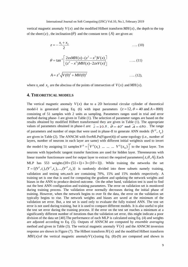
method and given in Table (3). The vertical magnetic anomaly ( )V x and the ANNCM inversion

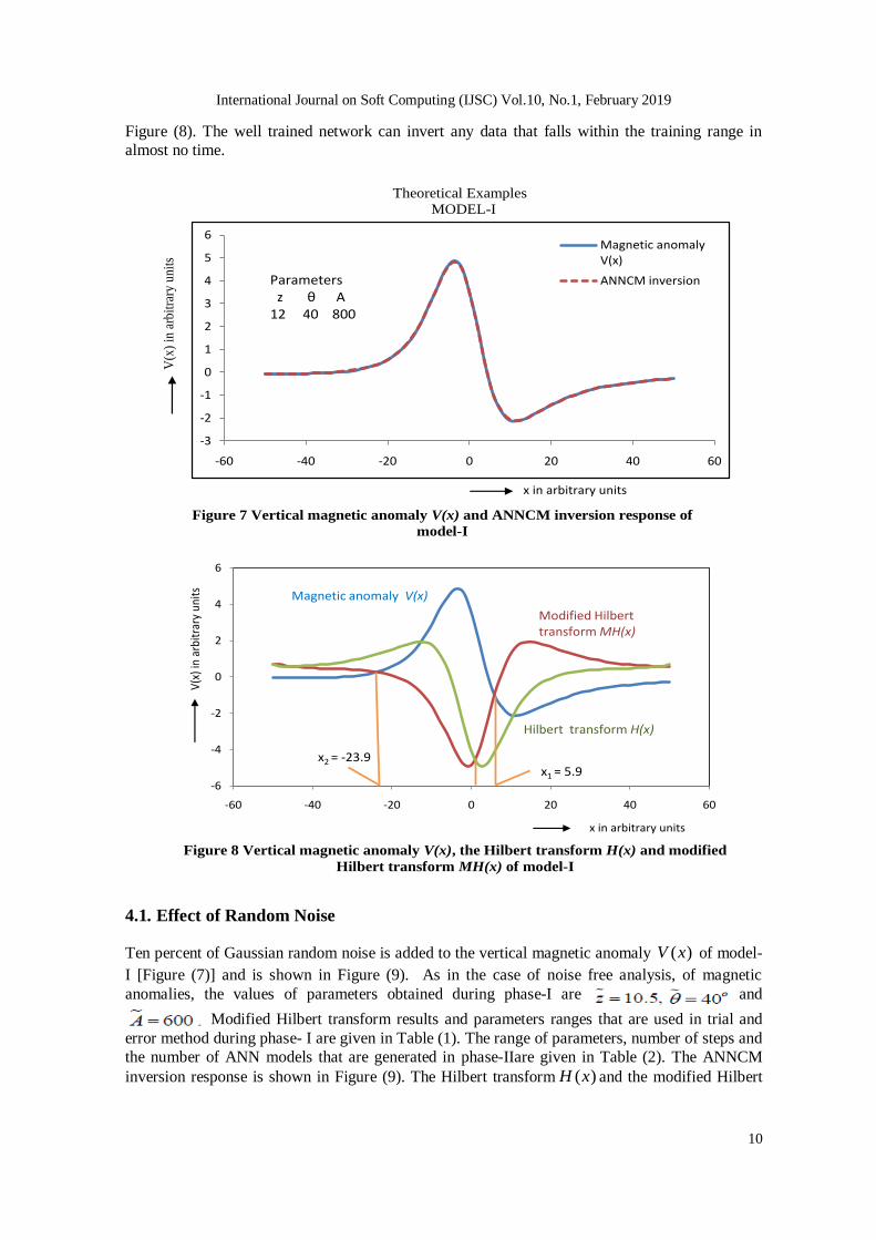
response are shown in Figure (7). The Hilbert transform ( )H x and the modified Hilbert transform

( )MH x of the vertical magnetic anomaly ( )V x using Eq. (8)-(9) are computed and shown in


10

Figure (8). The well trained network can invert any data that falls within the training range in

almost no time.

4.1. Effect of Random Noise

Ten percent of Gaussian random noise is added to the vertical magnetic anomaly ( )V x of model-

I [Figure (7)] and is shown in Figure (9). As in the case of noise free analysis, of magnetic

anomalies, the values of parameters obtained during phase-I are and

Modified Hilbert transform results and parameters ranges that are used in trial and

error method during phase- I are given in Table (1). The range of parameters, number of steps and

the number of ANN models that are generated in phase-IIare given in Table (2). The ANNCM

inversion response is shown in Figure (9). The Hilbert transform ( )H x and the modified Hilbert

Theoretical Examples

MODEL-I

Figure 7 Vertical magnetic anomaly V(x) and ANNCM inversion response of

model-I

V(x

) in

arb

itra

ry u

nit

s

x in arbitrary units

-3

-2

-1

0

1

2

3

4

5

6

-60 -40 -20 0 20 40 60

Magnetic anomaly V(x)

ANNCM inversionParametersz θ A

12 40 800

Figure 8 Vertical magnetic anomaly V(x), the Hilbert transform H(x) and modified

Hilbert transform MH(x) of model-I

V(x

) in

arbi

trar

y un

its

-6

-4

-2

0

2

4

6

-60 -40 -20 0 20 40 60


Modified Hilbert transform MH(x)

Hilbert transform H(x)

x2 = -23.9x1 = 5.9



11

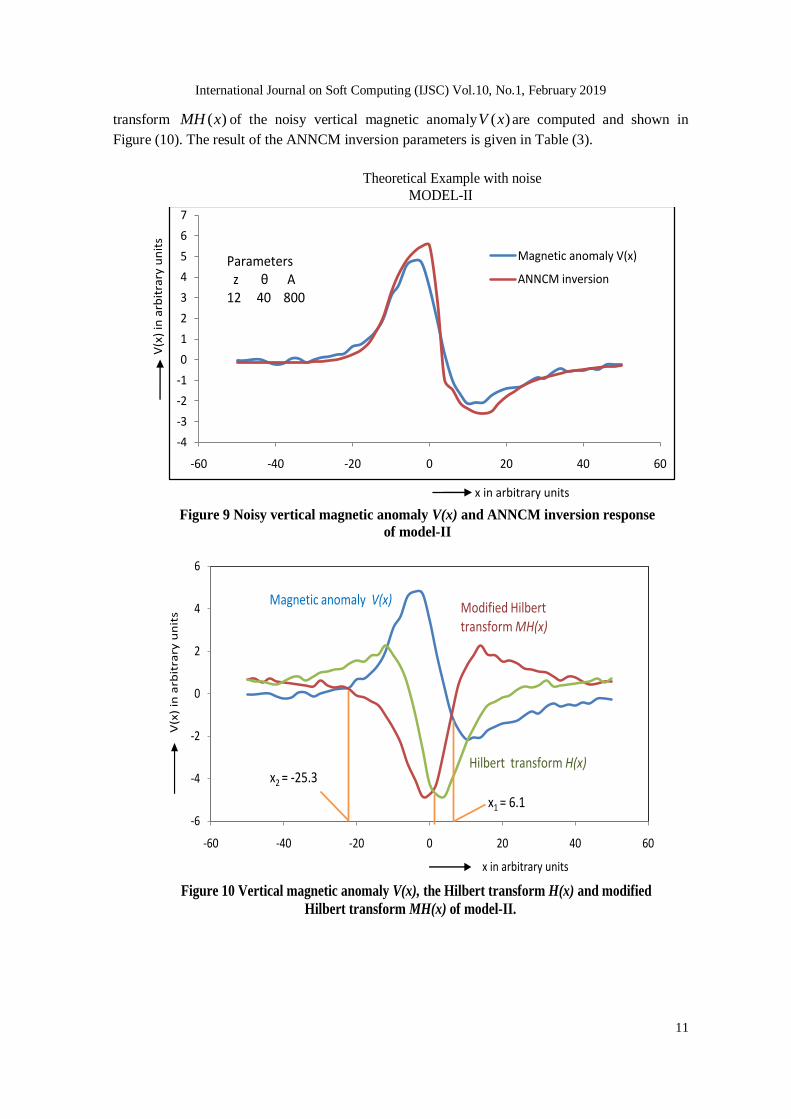
transform ( )MH x of the noisy vertical magnetic anomaly ( )V x are computed and shown in

Figure (10). The result of the ANNCM inversion parameters is given in Table (3).

Figure 10 Vertical magnetic anomaly V(x), the Hilbert transform H(x) and modified

Hilbert transform MH(x) of model-II.

-6

-4

-2

0

2

4

6

-60 -40 -20 0 20 40 60

Magnetic anomaly V(x)Modified Hilbert transform MH(x)

Hilbert transform H(x)x2 = -25.3

x1 = 6.1


V(x

) in

arb

itra

ry u

nit

s

Theoretical Example with noise

MODEL-II


Figure 9 Noisy vertical magnetic anomaly V(x) and ANNCM inversion response

of model-II

V(x

) in

arb

itra

ry u

nit

s

-4

-3

-2

-1

0

1

2

3

4

5

6

7

-60 -40 -20 0 20 40 60


ANNCM inversion

Parametersz θ A

12 40 800


12

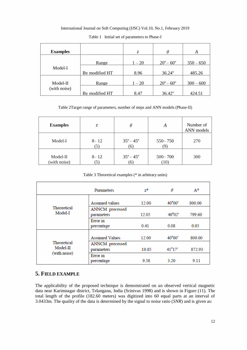
Table 1 Initial set of parameters to Phase-I

Examples

z

A

Model-I

Range

1 – 20

20o – 60o

350 – 650

By modified HT

8.96

36.24o

485.26

Model-II

(with noise)

Range

1 – 20

20o – 60o

300 – 600 By modified HT

8.47

36.42o

424.51

Table 2Target range of parameters, number of steps and ANN models (Phase-II)

Examples

z

A

Number of

ANN models

Model-I

8– 12

(5)

35o – 45o

(6)

550– 750

(9)

270

Model-II

(with noise)

8– 12

(5)

35o – 45o

(6)

500– 700

(10)

300

Table 3 Theoretical examples (* in arbitrary units)

5. FIELD EXAMPLE

The applicability of the proposed technique is demonstrated on an observed vertical magnetic data near Karimnagar district, Telangana, India (Srinivas 1998) and is shown in Figure (11). The

total length of the profile (182.60 meters) was digitized into 60 equal parts at an interval of

3.0433m. The quality of the data is determined by the signal to noise ratio (SNR) and is given as:


13

mSNR

s ,

where m is the mean and s is the standard deviation of the data. If the ratio is less than 3, the data

is assumed to be very poor quality. If the ratio is greater than 3, then the level of noise is

negligible and the data shall be considered clean. Signal to noise ratio of the field datais

calculated and is given by:

5017.17.7567

646.8136SNR

The parameters ranges that were used in trial and error method during phase-I obtained by

modified Hilbert transform and are given as:

the depth z (19m–50m)

the inclination ( 1o–150o)

the constant A (450,00,000–550,00,000)

The appropriate values of parameters obtained in phase-I are

Three hundred training models were created by assigning different values to

( , , )z A in a close range of which were used in phase-II are as follows:

the depth z (19m – 29m), with five points in this range

the inclination (70o – 80o), with six points in this range

the constant A (465,62,000 – 466,22,000), with ten points in this range;

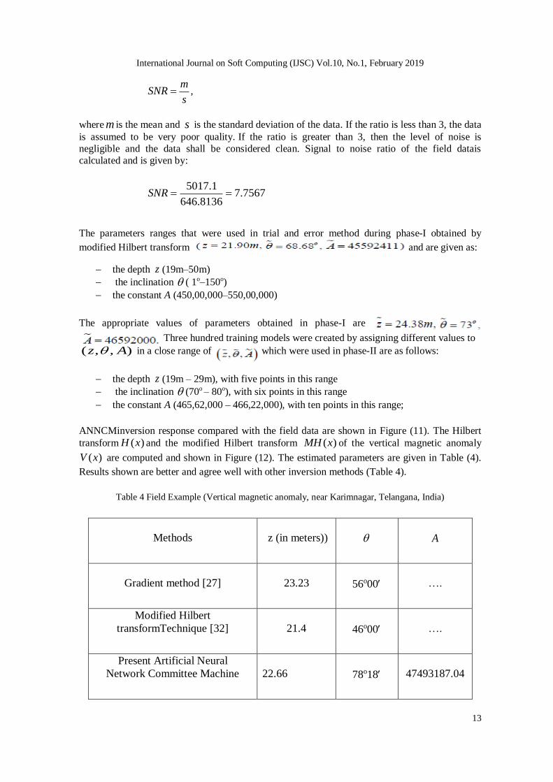
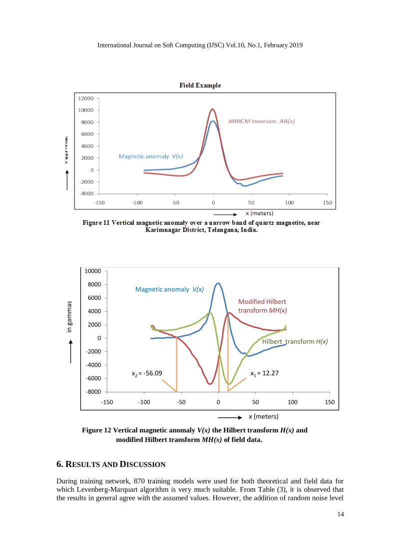
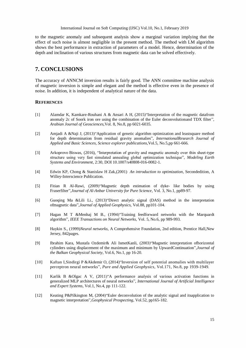
ANNCMinversion response compared with the field data are shown in Figure (11). The Hilbert

transform ( )H x and the modified Hilbert transform ( )MH x of the vertical magnetic anomaly

( )V x are computed and shown in Figure (12). The estimated parameters are given in Table (4).

Results shown are better and agree well with other inversion methods (Table 4).

Table 4 Field Example (Vertical magnetic anomaly, near Karimnagar, Telangana, India)

Methods

z (in meters))

A

Gradient method [27]

23.23

56o00

….

Modified Hilbert

transformTechnique [32]

21.4

46o00

….

Present Artificial Neural

Network Committee Machine

22.66

78o18

47493187.04


14

6. RESULTS AND DISCUSSION

During training network, 870 training models were used for both theoretical and field data for which Levenberg-Marquart algorithm is very much suitable. From Table (3), it is observed that

the results in general agree with the assumed values. However, the addition of random noise level

Figure 12 Vertical magnetic anomaly V(x) the Hilbert transform H(x) and

modified Hilbert transform MH(x) of field data.

in g

amm

as

x (meters)

-8000

-6000

-4000

-2000

0

2000

4000

6000

8000

10000

-150 -100 -50 0 50 100 150


Modified Hilbert transform MH(x)

Hilbert transform H(x)

x2 = -56.09 x1 = 12.27


15

to the magnetic anomaly and subsequent analysis show a marginal variation implying that the

effect of such noise is almost negligible in the present method. The method with LM algorithm

shows the best performance in extraction of parameters of a model. Hence, determination of the

depth and inclination of various structures from magnetic data can be solved effectively.

7. CONCLUSIONS

The accuracy of ANNCM inversion results is fairly good. The ANN committee machine analysis of magnetic inversion is simple and elegant and the method is effective even in the presence of

noise. In addition, it is independent of analytical nature of the data.

REFERENCES

[1] Alamdar K, Kamkare-Rouhani A & Ansari A H, (2015)“Interpretation of the magnetic datafrom

anomaly 2c of Soork iron ore using the combination of the Euler deconvolutionand TDX filter”,

Arabian Journal of Geosciences,Vol. 8, No.8, pp 6021-6035.

[2] Amjadi A &Naji J, (2013)“Application of genetic algorithm optimization and leastsquare method

for depth determination from residual gravity anomalies”, InternationalResearch Journal of

Applied and Basic Sciences, Science explorer publications,Vol.5, No.5,pp 661-666.

[3] Arkoprovo Biswas, (2016), “Interpretation of gravity and magnetic anomaly over thin sheet-type

structure using very fast simulated annealing global optimization technique”, Modeling Earth

Systems and Environment, 2:30, DOI 10.1007/s40808-016-0082-1.

[4] Edwin KP, Chong & Stanislaw H Zak,(2001) An introduction to optimization, Secondedition, A

Willey-Interscience Publication.

[5] Fitian R Al-Rawi, (2009)“Magnetic depth estimation of dyke- like bodies by using

Fraserfilter”,Journal of Al-Anbar University for Pure Science, Vol. 3, No.1, pp89-97.

[6] Guoqing Ma &Lili Li., (2013)“Direct analytic signal (DAS) method in the interpretation

ofmagnetic data”,Journal of Applied Geophysics, Vol.88, pp101-104.

[7] Hagan M T &Menhaj M B., (1994)“Training feedforward networks with the Marquardt

algorithm”, IEEE Transactions on Neural Networks, Vol. 5, No.6, pp 989-993.

[8] Haykin S., (1999)Neural networks, A Comprehensive Foundation, 2nd edition, Prentice Hall,New

Jersey, 842pages.

[9] Ibrahim Kara, Mustafa Ozdemir& Ali IsmetKanli, (2003)“Magnetic interpretation ofhorizontal

cylinders using displacement of the maximum and minimum by UpwardContinuation”,Journal of

the Balkan Geophysical Society, Vol.6, No.1, pp 16-20.

[10] Kaftan I,Sindirgi P &Akdemir O, (2014)“Inversion of self potential anomalies with multilayer

perceptron neural networks”, Pure and Applied Geophysics, Vol.171, No.8, pp 1939-1949.

[11] Karlik B &Olgac A V, (2011)“A performance analysis of various activation functions in

generalized MLP architectures of neural networks”, International Journal of Artificial Intelligence

and Expert Systems, Vol.1, No.4, pp 111-122.

[12] Keating P&Pilkington M, (2004)“Euler deconvolution of the analytic signal and itsapplication to

magnetic interpretation”,Geophysical Prospecting, Vol.52, pp165-182.

https://link.springer.com/journal/40808

https://link.springer.com/journal/40808

http://www.sciencedirect.com/science/journal/09269851

http://link.springer.com/search?facet-author=%22%C3%96zer+Akdemir%22


16

[13] Krasnopolsky V M, (2007)“Reducing uncertainties in neural network Jacobians andimproving

accuracy of neural network emulations with ensemble approaches”, NeuralNetworks, Vol.20, No.4, pp 454-461.

[14] Lashin A & Din S S El, (2013)“Reservoir parameters determination using artificial neural

networks: RasFanar field, Gulf of Suez, Egypt”, Arabian Journal of Geosciences, Vol.6, No.8, pp

2789-2806.

[15] Levenberg K, (1944)“A method for the solution of certain nonlinear problems in least

squares”,Quarterly of Applied Mathematics, Vol.2, pp164-168.

[16] Li Y & Oldenburg DW, (2003)“Fast inversion of large scale magnetic data using

wavelettransforms and a logarithmic barrier method”,Geophysical Journal International, Vol.152,

pp251-265.

[17] Mansour A Al-Garni, (2009)“Interpretation of some magnetic bodies using neuralnetworks

inversion”, Arabian Journal of Geosciences, Vol.2, No.2, pp 175-184.

[18] Mansour A Al-Garni, (2011)“Spectral analysis of magnetic anomalies due to a 2-D

horizontalcircular cylinder, A Hartley transforms technique”,SQU Journal for Science, Vol.16,pp

45-56.

[19] Marquardt D, (1963)“An algorithm for least-squares estimation of nonlinear parameters”,Journal

of the Society for Industrial and Applied Mathematics, Vol.11, No.2, pp 431-441.

[20] McCulloch W S & Pitts W, (1943)“A logical calculus for ideas imminent in nervous activity”, Bulletin of Mathematical Biophysics, Vol. 5, pp 115-133.

[21] Mohan NL, Babu L, Sundararajan N&SeshagiriRao SV, (1990)“Analysis of magneticanomalies

due to some two dimensional bodies using the Mellin transform”,Pure andApplied Geophysics,

Vol.133, pp 403-428.

[22] Moreau F, Gilbert D, Holschneider M &Saracco G, (1999)“Identification of sources ofpotential

fields with continuous wavelet transform,Basic theory”,J. Geophys. Res,Vol.104, pp5003-5013.

[23] Murthy KSR& Mishra DC, (1980)“Fourier transform of the general expression for themagnetic

anomaly due to long horizontal cylinder”,Geophysics, Vol.45, pp 1091-1093.

[24] Naftaly U, Intrator N & Horn D, (1997)“Optimal ensemble averaging of neural

networks”,Network: Computation in Neural Systems, Vol.8, pp 283-296.

[25] Parker Gay Jr.S, (1965)“Standard curves for magnetic anomalies over long

horizontalcylinders”,Geophysics, Vol.30, pp 818-828.

[26] Pourghasemi H R, Pradhan B &Gokceoglu C, (2012)“Application offuzzy logic andanalytical

hierarchy process (AHP) to landslide susceptibilitymapping at Harazwatershed, Iran”, Natural

Hazards., Vol.63, No.2, pp 965-996.

[27] RadhakrishnaMurthy I V, VisweswaraRao C &Gopala Krishna C, (1980)“A gradient method for interpreting magnetic anomalies due to horizontal circular cylinders, infinite dykes and vertical

steps”,Journal of Earth System Science, Vol. 89, No. 1, pp31-42.

[28] Rao BSR, RadhaKrishna Murthy IV&VisweswaraRao, (1973)“A direct method ofinterpreting

gravity and magnetic anomalies, The case of a horizontal cylinder”,PAGEOPH, Vol.102, pp 67-

72.

[29] Rosenblatt F, (1958)“The perceptron: A probabilistic model for information storage and

organization in the brain”, Psychological Review, Vol. 65, pp 386-408.

http://link.springer.com/journal/12517




17

[30] SaumenMaiti, Vinit C Erram, Gautam Gupta & Ram Krishna Tiwari, (2012)“ANN basedinversion

of DC resistivity data for groundwater exploration in hard rock terrain ofwestern Maharashtra (India)”. Journal of Hydrology, Vols.464–465: pp294-308.

[31] Sibi P, Allwyn Jones S&Siddarth P, (2013)“Analysis of different activation functions usingback

propagation neural networks”,Journal of Theoretical and Applied InformationTechnology, Vol.47,

No.3, pp 1264-1268.

[32] Srinivas Y., (1998)Modified Hilbert transform- A tool to the interpretation of geopotentialfield

anomalies, Thesis, Osmania University, Hyderabad, India.

[33] Srinivas Y, Stanley Raj A, Muthuraj D,Hudson Oliver D &Chandrasekar N,(2010)“Anapplication

of artificial neural network for the interpretation of three layer electricalresistivity data using feed

forward back propagation algorithm”,Current Developmentin Artificial Intelligence, Vol.1, No.1-3, pp 1-11.

[34] Sundararajan N, Mohan NL, VijayaRaghava MS&SeshagiriRao SV, (1985)“Hilberttransform in

the interpretation of magnetic anomalies of various components due tothin infinite

dyke”,PAGEOPH, Vol.123, pp557-566.

[35] Sundararajan N, Umashankar B, Mohan NL&SeshagiriRao SV, (1989)“Directinterpretation of

magnetic anomalies due to spherical sources-A Hilbert transformmethod”,Geophysical

Transactions, Vol.35, No.3, pp 507-512.

[36] Sundararajan N &Srinivas Y, (1996)“A modified Hilbert transform and its applications toself-potential interpretation”, Journal of Applied Geophysics, Vol.36, pp. 137-143.

[37] Sundararajan N, Srinivas Y&LaxminarayanaRao T,(2000)“Sundararajan Transform – a tool to

interpret potential field anomalies”, Exploration Geophysics, Vol. 31, No. 4, pp622-628.

[38] M.Tavakoli, A.NejatiKalateh&S.Ghomi, 2016, “The interpretation of magnetic anomalies by 3D

inversion: A case study from Central Iran”, Journal of African Earth Sciences, Vol 115, pp. 85-91.

[39] YunusLeventEkinci, ŞenolÖzyalın, PetekSındırgı, ÇağlayanBalkaya&GökhanGöktürkler, (2017),

“Amplitude inversion of the 2D analytic signal of magnetic anomalies through the differential

evolution algorithm”, Journal of Geophysics and Engineering, Vol. 14, pp. 1492-1508.

[40] Wenyan Wu, Robert May, Graeme C Dandy&Holger R Maier., (2012), “A method forcomparing

data splitting approaches for developing hydrological ANN models”,International Environmental

Modelling and Software Society, 2012, Proceedingof the International Congress on Environmental

Modelling and Software: Managing Resources of a Limited Planet, 6th Biennial Meeting, held in

Leipzig,Germany, Seppelt R,Voinov A.A, Lange S &Bankamp D. (Eds.), pp. 1 – 8.

Authors Biography Dr. M. Bhagwan Das post graduated in Mathematics from the Kakatiya University with

gold medal followedM.Philfrom University of Hyderabad and Ph.D in Mathematics

from Osmania University, Hyderabad, India. He is currently head of the department,

Mathematics at SreeTriveni Educational Institutions, Hyderabad. He worked on an

inversion of geophysical problems using Neural Networks and Hilbert transformation

with Prof. N. Sundararajan. His research is centered on development of new algorithms,

Neural Networks, Wavelet Transforms, Fractals and their applications etc.

http://library.seg.org/action/doSearch?displaySummary=true&ContribStored=Sundararajan%2C+N

http://library.seg.org/action/doSearch?displaySummary=true&ContribStored=Srinivas%2C+Y

http://library.seg.org/action/doSearch?displaySummary=true&ContribStored=Rao%2C+T+Laxminarayana

https://www.sciencedirect.com/science/journal/1464343X


18

Dr.NarasimmanSundararajan graduated in Mathematics from the University of

Madras followed by an M.Sc(Tech) and Ph.D in Geophysics from Osmania University, India. Began a career as a Research Scientist and later switched over to

teaching in Osmania University where he became a Professor in 2004. Currently he is

in the Department of Earth Sciences, Sultan Qaboos University, Oman. Published

more than 90 research papers in the leading International journals besides a book and a

couple of Book chapters and supervised several Ph.Ds in Geophysics as well as

Mathematics. Brought out a few innovative tools for processing and interpreting of various geophysical

data besides mathematical concept called “Sundararajan Transform”.Implemented several research

projects including one on Uranium exploration. Member of XIV Indian Scientific Expedition to Antarctica

during 1994-95. Introduced a valid and viable approach to multidimensional Hartley transform in contrast

with the definition of Prof R N Bracewell from Stanford University, USA. For his overall significant

research contribution, Govt. of India has conferred upon him the National Award for Geosciences in 2007.

His research interests are varied and wide including geophysical data processing, mineral and ground water exploration, earth quake hazard assessment studies etc. In 2015, Dr.Sundararajan joined as an Associate

Editor of Arabian Journal of Geosciences(Springer) responsible for evaluating submission in the field of

theoretical and applied geophysics.

Documents

INVERSIONOF MAGNETIC ANOMALIES DUE TO 2-D CYLINDRICAL