1

MARINE MAGNETIC ANOMALIES(Copyright, 2001, David T. Sandwell)

Introduction

This lecture is basically the development of the equations needed to compute the scalar

magnetic field that would be recorded by a magnetometer towed behind a ship given a

magnetic timescale, a spreading rate, and a skewness. A number of assumptions are

made to simplify the mathematics. The intent is to first review the origin of natural

remnant magnetism (NRM) to illustrate that the magnetized layer is thin compared with

its horizontal dimension. Then the relevant differential equations are developed and

solved under the ideal case of seafloor spreading at the north magnetic pole. This

development highlights the fourier approach to the solution to linear partial differential

equations. The same approach will be used to develop the Green's functions for heat

flow, flexure, gravity, and elastic dislocation. For a more general development of the

geomagnetic solution, see the reference by Parker [1973].

Crustal Magnetization at a Spreading Ridge

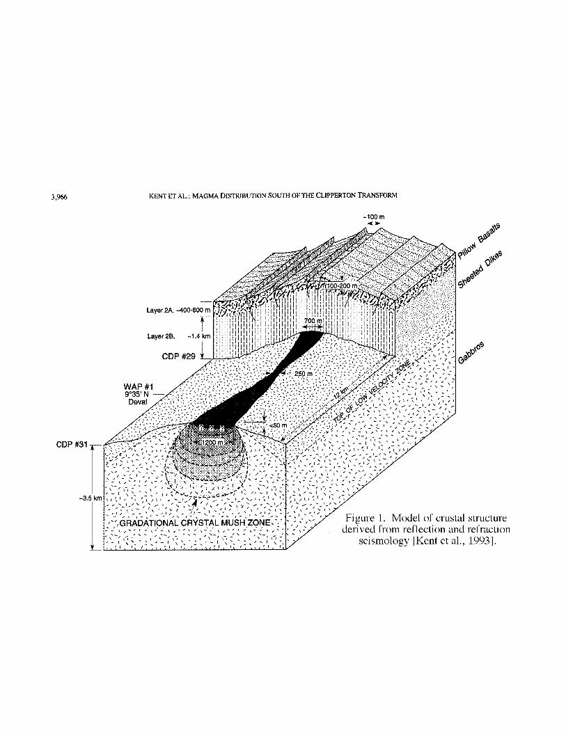
As magma is extruded at the ridge axis, its temperature falls below the Curie point and

the uppermost part of the crust becomes magnetized in the direction of the present-day

magnetic field. Figure 1 from Kent et al. [1993] illustrates the current model of crustal

generation. Partial melt that forms by pressure-release in the uppermost mantle (~40 km

depth) percolates to a depth of about 2000 m beneath the ridge where it accumulates to

form a thin magma lens. Beneath the lens is a mush-zone develops into a 3500-m thick

gabbro layer by some complicated ductile flow. Above the lens, sheeted dikes (~1400-

thick) are injected into the widening crack at the ridge axis. Part of this volcanism is

extruded into the seafloor as pillow basalts. The pillow basalts and sheeted dikes cool

rapidly below the Curie temperature as cool seawater percolates to a depth of at least

2000 m. This process forms the basic crustal layers seen by reflection and refraction

seismology methods.

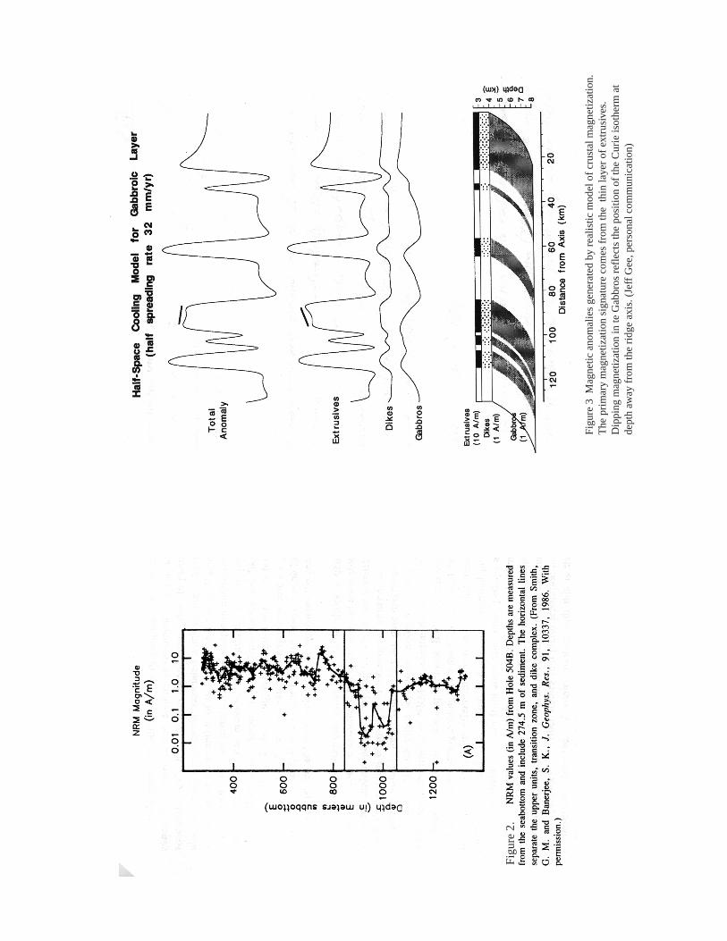
The highest magnetization occurs in the extrusive layer 2A (Figure 2) although the

Figu

re 2

.

Figu

re 3

Mag

netic

ano

mal

ies

gene

rate

d by

rea

listic

mod

el o

f cr

usta

l mag

netiz

atio

n.

The

pri

mar

y m

agne

tizat

ion

sign

atur

e co

mes

fro

m th

e th

in la

yer

of e

xtru

sive

s.

Dip

ping

mag

netiz

atio

n in

te G

abbr

os r

efle

cts

the

posi

tion

of th

e C

urie

isot

herm

at

dept

h aw

ay f

rom

the

ridg

e ax

is. (

Jeff

Gee

, per

sona

l com

mun

icat

ion)

4

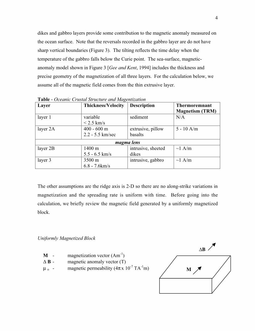
dikes and gabbro layers provide some contribution to the magnetic anomaly measured on

the ocean surface. Note that the reversals recorded in the gabbro layer are do not have

sharp vertical boundaries (Figure 3). The tilting reflects the time delay when the

temperature of the gabbro falls below the Curie point. The sea-surface, magnetic-

anomaly model shown in Figure 3 [Gee and Kent, 1994] includes the thickness and

precise geometry of the magnetization of all three layers. For the calculation below, we

assume all of the magnetic field comes from the thin extrusive layer.

Table - Oceanic Crustal Structure and MagentizationLayer Thickness/Velocity Description Thermoremnant

Magnetism (TRM)layer 1 variable

< 2.5 km/ssediment N/A

layer 2A 400 - 600 m2.2 - 5.5 km/sec

extrusive, pillowbasalts

5 - 10 A/m

magma lenslayer 2B 1400 m

5.5 - 6.5 km/sintrusive, sheeteddikes

~1 A/m

layer 3 3500 m6.8 - 7.6km/s

intrusive, gabbro ~1 A/m

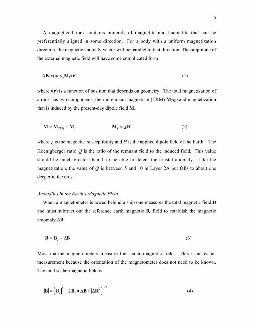
The other assumptions are the ridge axis is 2-D so there are no along-strike variations in

magnetization and the spreading rate is uniform with time. Before going into the

calculation, we briefly review the magnetic field generated by a uniformly magnetized

block.

Uniformly Magnetized Block

M - magnetization vector (Am-1)Δ B - magnetic anomaly vector (T)µ o - magnetic permeability (4π x 10-7 TA-1m)

ΔB

M

5

A magnetized rock contains minerals of magnetite and haematite that can be

preferentially aligned in some direction. For a body with a uniform magnetization

direction, the magnetic anomaly vector will be parallel to that direction. The amplitude of

the external magnetic field will have some complicated form

where f(r) is a function of position that depends on geometry. The total magnetization of

a rock has two components, thermoremnant magnetism (TRM) MTRM and magnetization

that is induced by the present-day dipole field MI.

where χ is the magnetic susceptibility and H is the applied dipole field of the Earth. The

Koenigberger ratio Q is the ratio of the remnant field to the induced field. This value

should be much greater than 1 to be able to detect the crustal anomaly. Like the

magnetization, the value of Q is between 5 and 10 in Layer 2A but falls to about one

deeper in the crust.

Anomalies in the Earth's Magnetic Field

When a magnetometer is towed behind a ship one measures the total magnetic field B

and must subtract out the reference earth magnetic Be field to establish the magnetic

amomaly ΔB.

Most marine magnetometers measure the scalar magnetic field. This is an easier

measurement because the orientation of the magnetometer does not need to be known.

The total scalar magnetic field is

ΔB(r) = µoMf (r) (1)

M =MTRM +MI MI = χH (2)

B = Be + ΔB (3)

B = Be2+ 2Be • ΔB+ ΔB 2( )1 / 2

(4)

6

The dipolar field of the earth is typically 50,000 nT while the crustal anomalies are only

about 300 nT. Thus |ΔB|2 is small relative to the other terms and we can develop an

approximate formula for the total scalar field.

Equation (5) can be re-arranged to relate the measured scalar anomaly A to the vector

anomaly ΔB given an independent measurement of the dipolar field of the earth Be.

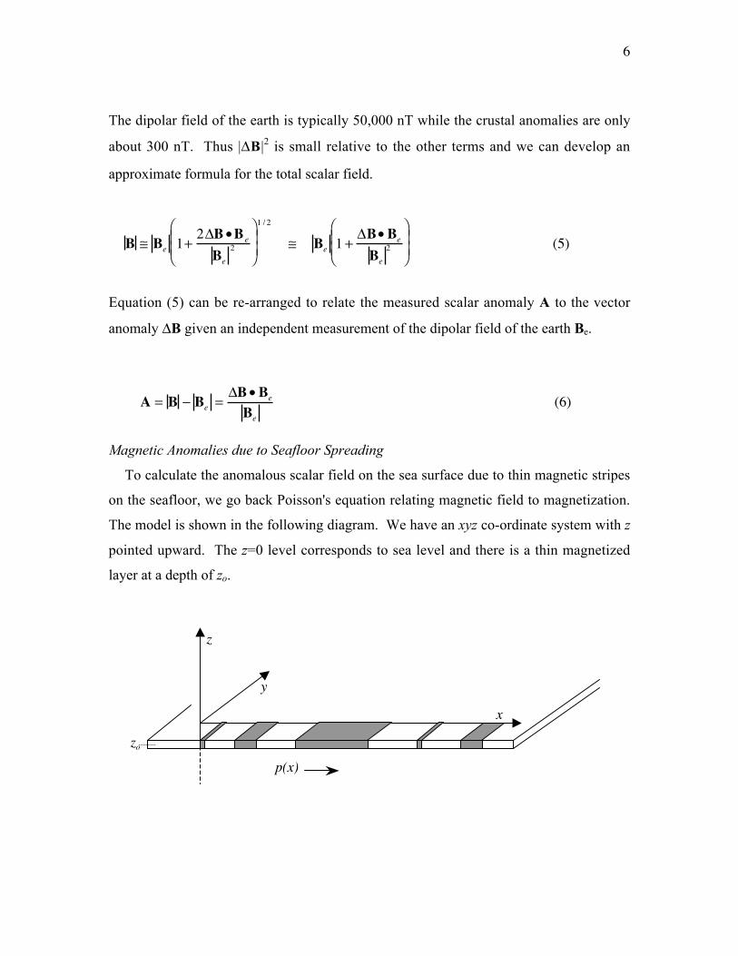
Magnetic Anomalies due to Seafloor Spreading

To calculate the anomalous scalar field on the sea surface due to thin magnetic stripes

on the seafloor, we go back Poisson's equation relating magnetic field to magnetization.

The model is shown in the following diagram. We have an xyz co-ordinate system with z

pointed upward. The z=0 level corresponds to sea level and there is a thin magnetized

layer at a depth of zo.

B ≅ Be 1+2ΔB•B e

Be2

⎛

⎝ ⎜ ⎜

⎞

⎠ ⎟ ⎟

1 / 2

≅ Be 1 +ΔB• Be

Be2

⎛

⎝ ⎜ ⎜

⎞

⎠ ⎟ ⎟ (5)

A = B − Be =ΔB• Be

Be

(6)

z

y

x

zo

p(x)

7

We define a scalar potential U and a magnetization vector M. The magnetic anomaly ΔB

is the negative gradient of the potential. The potential satisfies Laplace's equation above

the source layer and is satisfies Poisson's equation within the source layer.

U(x,y,z) - magnetic potential Tmµo - magnetic permeability TA-1 m = 4πx10-7

M - magnetization vector Am-1

In addition to assuming the layer is infinitesimally thin, we assume that the magnetization

direction is constant but that the magnetization varies in strength and polarity as specified

by the reversal function p(x). The approach to the solution is:

i) solve the differential equation and calculate the magnetic potential U at z=0.

ii) calculate the magnetic anomaly vector ΔB.

iii) calculate the scalar magnetic field A = (ΔB • Be)/|Be| .

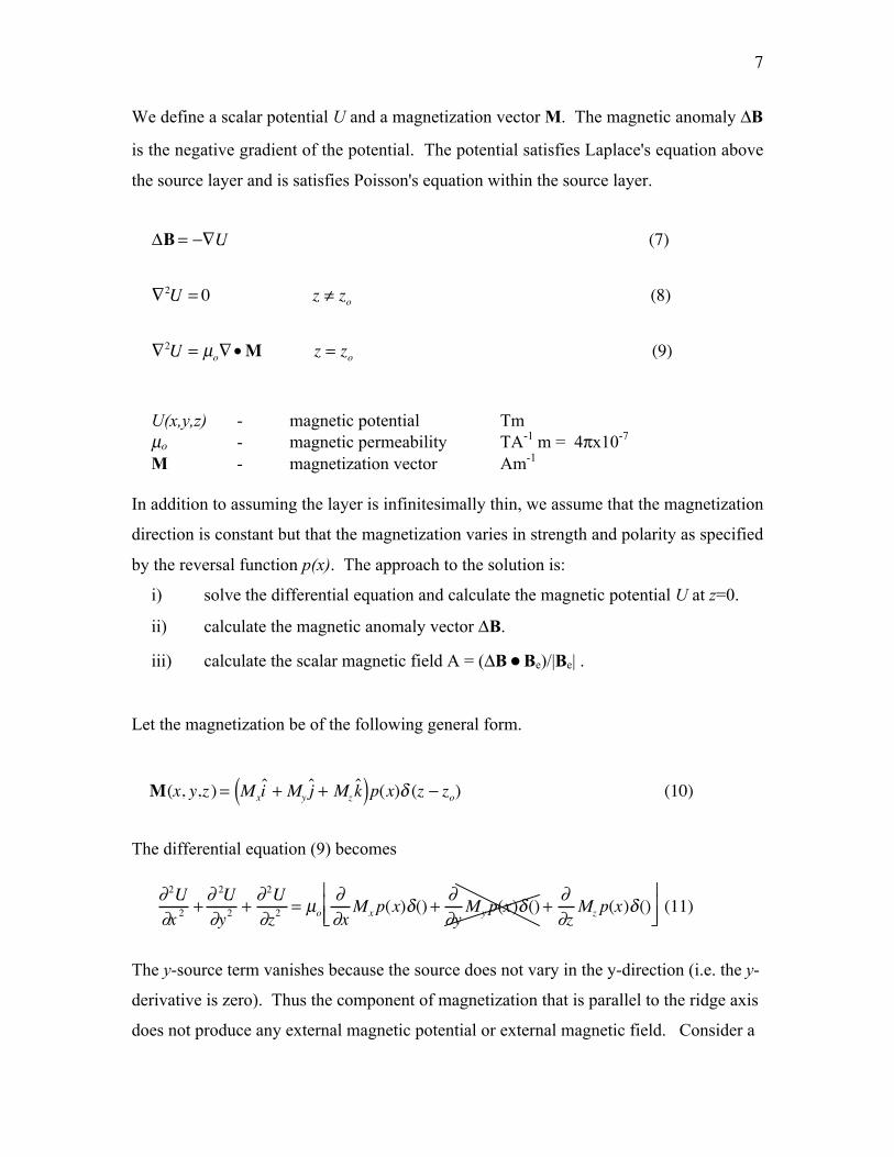
Let the magnetization be of the following general form.

The differential equation (9) becomes

The y-source term vanishes because the source does not vary in the y-direction (i.e. the y-

derivative is zero). Thus the component of magnetization that is parallel to the ridge axis

does not produce any external magnetic potential or external magnetic field. Consider a

ΔB = −∇U (7)

∇2U = 0 z ≠ zo (8)

∇2U = µo∇•M z = zo (9)

∂ 2U∂x 2 +

∂ 2U∂y2 +

∂ 2U∂z2 = µo

∂∂xMx p(x)δ() +

∂∂yMy p(x)δ() +

∂∂zMz p(x)δ()

⎡

⎣ ⎢ ⎢

⎤

⎦ ⎥ ⎥ (11)

M(x, y,z ) = Mxˆ i + My

ˆ j + Mzˆ k ( )p(x)δ (z − zo) (10)

8

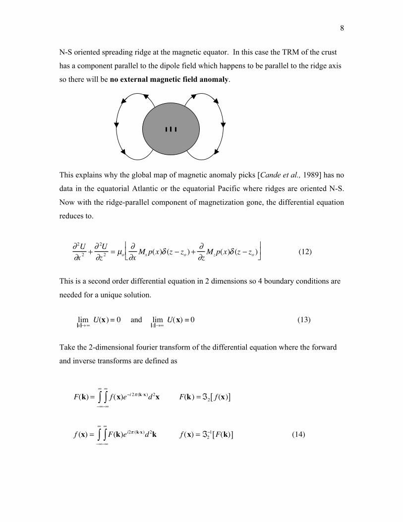
N-S oriented spreading ridge at the magnetic equator. In this case the TRM of the crust

has a component parallel to the dipole field which happens to be parallel to the ridge axis

so there will be no external magnetic field anomaly.

This explains why the global map of magnetic anomaly picks [Cande et al., 1989] has no

data in the equatorial Atlantic or the equatorial Pacific where ridges are oriented N-S.

Now with the ridge-parallel component of magnetization gone, the differential equation

reduces to.

This is a second order differential equation in 2 dimensions so 4 boundary conditions are

needed for a unique solution.

Take the 2-dimensional fourier transform of the differential equation where the forward

and inverse transforms are defined as

F(k) = f (x−∞

∞

∫−∞

∞

∫ )e−i 2π (k ⋅x )d2x F(k) =ℑ2 f (x)[ ]

f (x) = F(k−∞

∞

∫−∞

∞

∫ )ei2π (k⋅x )d2k f (x) = ℑ2−1 F(k)[ ] (14)

∂ 2U∂x 2 +

∂ 2U∂z 2 = µo

∂∂x

Mx p(x)δ (z − zo ) +∂∂zMzp(x)δ (z − zo )

⎡ ⎣ ⎢

⎤ ⎦ ⎥ (12)

limx→∞

U(x ) = 0 and limz →∞

U(x) = 0 (13)

9

where x = (x, z) is the position vector, k = (kx, kz) is the wavenumber vector, and

(k . x) = kx x + kz z. The derivative property is ℑ2[dU/dx] = i2πkx ℑ2[U]. The fourier

transform of the differential equation is.

The fourier transform in the z-direction was done using the following identity.

Now we can solve for U(k)

Next, take the inverse fourier transform with respect to kz using the Cauchy Residue

Theorem (below).

The poles of the integrand are found by factoring the denominator.

We see that U(k) is an analytic function with poles at +ikx. The integral of this function

about any closed path in the complex kz plane is zero unless the contour includes a pole in

which case the integral is i2π times the residue at the pole.

δ z − zo( )−∞

∞

∫ e− i2πk zz dz ≡ e− i2πk z zo (16)

U(k) = -iµo

2πp(kx)(k•M) e

−i 2πkz zo

kx2 + kz

2( ) (17)

U(kx, z) = µo

2πip(kx ) (k •M)ei 2πkz (z− zo )

kx2 + kz

2( )−∞

∞

∫ dkz (18)

kx2 + kz

2 = (kz + ikx)(kz − ikx) (19)

f (z)z − zo

dz = i2πf (zo∫ ) (20)

− 2πkx( )2+ 2πkz( )2[ ]U(kx ,kz ) = µo p(kx)e

−i 2πkz zo i2πk •M( ) (15)

10

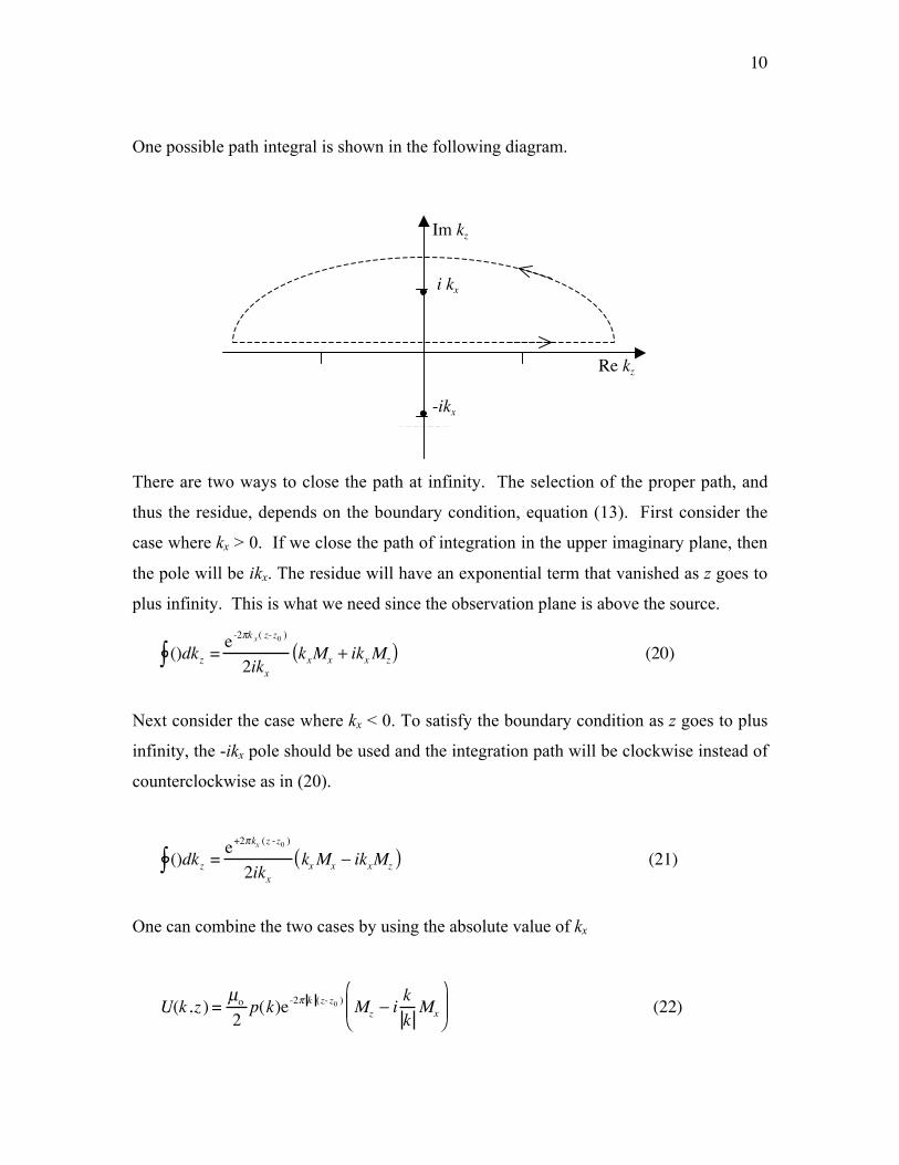
One possible path integral is shown in the following diagram.

There are two ways to close the path at infinity. The selection of the proper path, and

thus the residue, depends on the boundary condition, equation (13). First consider the

case where kx > 0. If we close the path of integration in the upper imaginary plane, then

the pole will be ikx. The residue will have an exponential term that vanished as z goes to

plus infinity. This is what we need since the observation plane is above the source.

Next consider the case where kx < 0. To satisfy the boundary condition as z goes to plus

infinity, the -ikx pole should be used and the integration path will be clockwise instead of

counterclockwise as in (20).

One can combine the two cases by using the absolute value of kx

Im kz

i kx

Re kz

-ikx

()dkz∫ = e-2πk x ( z- z0 )

2ikxkxMx + ikxMz( ) (20)

()dkz∫ = e+2πkx (z -z0 )

2ikxkxMx − ikxMz( ) (21)

U(k ,z ) = µo

2p(k)e-2π k (z- z0 ) Mz − i

kkMx

⎛

⎝ ⎜ ⎜

⎞

⎠ ⎟ ⎟ (22)

11

where we have dropped the subscript on the x-wavenumber.

This is the general case of an infinitely-long ridge. To further simplify the problem,

lets assume that this spreading ridge is located at the magnetic pole of the earth so the

dipolar field lines will be parallel to the z-axis and there will be no x-component of

magnetization. The result is.

Next calculate the magnetic anomaly ΔB = -∇U.

The scalar magnetic field is given by equation (6) and since only the z-component of the

earth's field is non-zero, the anomaly simplifies to.

observed = reversal x earth anomaly pattern filter

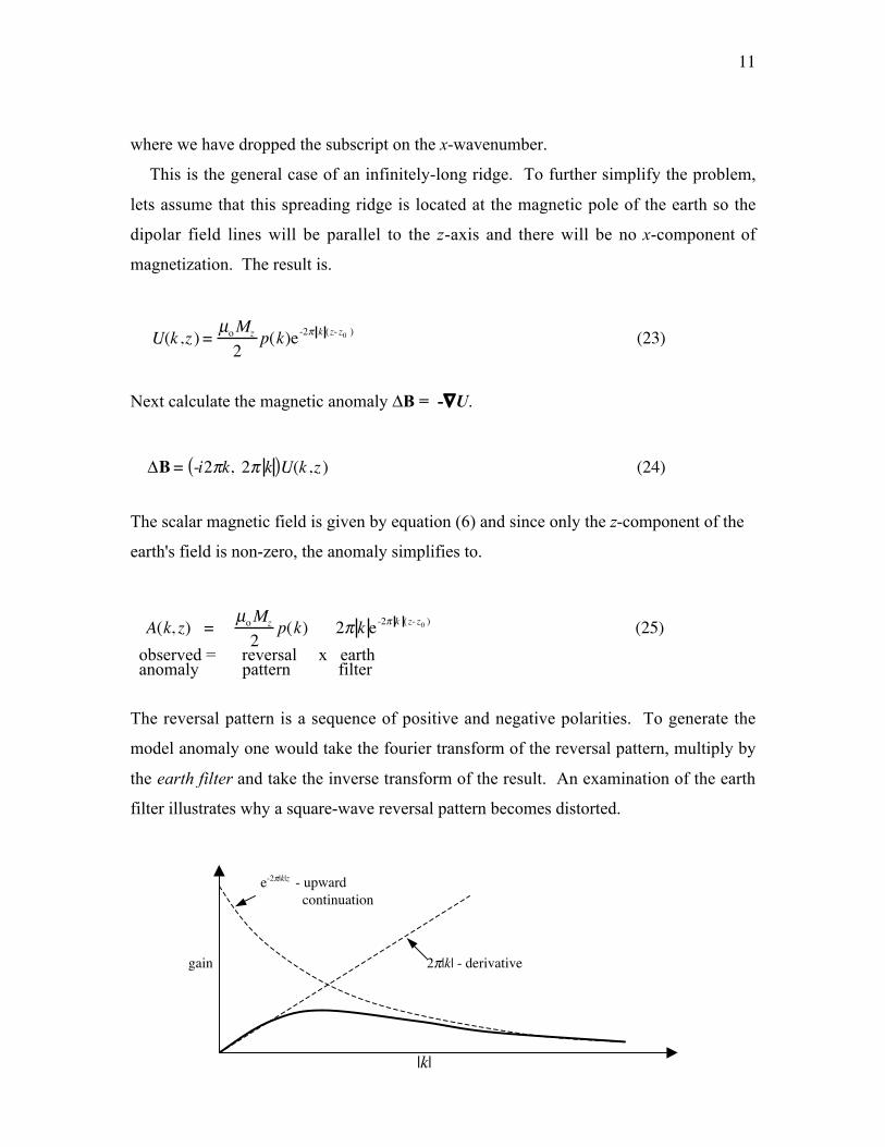
The reversal pattern is a sequence of positive and negative polarities. To generate the

model anomaly one would take the fourier transform of the reversal pattern, multiply by

the earth filter and take the inverse transform of the result. An examination of the earth

filter illustrates why a square-wave reversal pattern becomes distorted.

e-2π|k|z - upward continuation

gain 2π|k| - derivative

|k|

U(k ,z ) = µoMz

2p(k)e-2π k (z- z0 ) (23)

ΔB= -i2πk, 2π k( )U(k ,z ) (24)

A(k, z) = µoMz

2p(k) 2π k e-2π k (z- z0 ) (25)

12

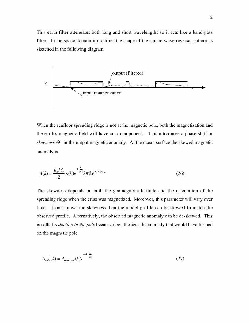
This earth filter attenuates both long and short wavelengths so it acts like a band-pass

filter. In the space domain it modifies the shape of the square-wave reversal pattern as

sketched in the following diagram.

When the seafloor spreading ridge is not at the magnetic pole, both the magnetization and

the earth's magnetic field will have an x-component. This introduces a phase shift or

skewness Θ, in the output magnetic anomaly. At the ocean surface the skewed magnetic

anomaly is.

The skewness depends on both the geomagnetic latitude and the orientation of the

spreading ridge when the crust was magnetized. Moreover, this parameter will vary over

time. If one knows the skewness then the model profile can be skewed to match the

observed profile. Alternatively, the observed magnetic anomaly can be de-skewed. This

is called reduction to the pole because it synthesizes the anomaly that would have formed

on the magnetic pole.

output (filtered)

A x input magnetization

Apole(k) = Aobserved (k )e− iΘ k

k (27)

A(k) = µoMz

2p(k)e

iΘ kk 2π k e+2π k z0 (26)

13

Discussion

The ability to observed magnetic reversals from a magnetometer towed behind a ship

relies on some rather incredible coincidences related to reversal rate, spreading rate,

ocean depth, and Earth temperatures, (mantle, seafloor, and Curie). In the case of marine

magnetic anomalies, four scales must match.

First the temperature of the mantle (1200˚C), the seafloor (0˚C), and the Curie

temperature of basalt (~500 ˚C) must be just right for recording the direction of the

Earth's magnetic field at the seafloor spreading ridge axis. Most of the thermoremnant

magnetism (TRM) is recorded in the upper 1000 meters of the oceanic crust. If the

thickness of the TRM layer was too great, then as the plate cools while it moves off the

spreading ridge axis, the positive and negative reversals would be juxtaposed in dipping

vertical layers (Figure 3); this superposition would smear the pattern observed by a ship.

If the seafloor temperature was above the Curie temperature, as it is on Venus, then no

recording would be possible.

The second scale is related to ocean depth and thus the earth filter. The external

magnetic field is the derivative of the magnetization which, as shown above, acts as a

high-pass filter applied to the reversal pattern recorded in the crust. The magnetic field

measured at the ocean surface will be naturally smooth (upward continuation) due to the

distance from the seafloor to the sea surface; this is a low-pass filter. This smoothing

depends exponentially on ocean depth so, for a wavelength of 2π times the mean ocean

depth, the field amplitude will be attenuated by 1/e or 0.37 with respect to the value

measured at the seafloor. The combined result of the derivative and the upward

continuation is a band-pass filter with a peak response at a wavelength of 2π times the

mean ocean depth or about 25-km. Wavelengths that are shorter (< 10 km) or much

longer (> 500 km) than this value will be undetectable at the ocean surface.

The third and fourth scales that must match are the reversal rate and the seafloor-

spreading rate. Half-spreading rates on the Earth vary from 10 to 80 km per million

years. Thus for the magnetic anomalies to be most visible on the ocean surface, the

reversal rate should be between 2.5 and 0.3 million years. It is astonishing that this is the

typical reversal rate observed in sequences of lava flows on land!! While most ocean

basins display clear reversal patterns, there was a period between 85 and 120 million

14

years ago when the magnetic field polarity of the Earth remained positive so the ocean

surface anomaly is too far from the reversal boundaries to provide timing information.

This area of seafllor is called the Cretaceous Quiet Zone and it is a problem area for

accurate plate reconstructions.

The lucky convergence of length and time scales makes it very unlikely that magnetic

anomalies, due to crustal spreading, will ever be observed on the other planet. This is the

main reason that I do not believe the recent publication that interprets the Martian field as

ancient spreading anomalies - one cannot be this lucky twice!

ReferencesBlakley, J., Potential Theory in Gravity and Magentics, Cambridge University Press,

New York, 1995.Cande, S.C., LaBrecque, J.L., Larson, R.L., Pitman, W.C., Golovchenko, X., and Haxby,

W.F., 1989. Magnetic Lineations of the World's Ocean Basins. Tulsa, OK.Phipps-Morgan, J., A. Harding, J. Orcutt, and Y.J. Chen, An Observational and

Theoretical Synthesis of Magma Chamber Geometry and Crustal Genesis along aMid-ocean Ridge Spreading Center, in Magmatic Systems, ed. M. P. Ryan,Academic Press, Inc., 1994. (Good review of crustal generation at mid-oceanridges.)

Fowler, C.M.R., The Solid Earth: An Introduction to Global Geophysics, CambridgeUniversity Press, 1990. (Marine magnetic anomalies and plate reconstructions -Chapter 3)

Gee, J and D. Kent, Variation in layer 2A thickness and the origin of the central anomalymagnetic high, Geophys. Res., Lett., v. 21, no. 4, 297-300, 1994.

Kent, G., A. Harding, J. Orcutt, Distribution of Magma Beneath the East Pacific RiseBetween the Clipperton Transform and the 9˚17' Deval From Forward Modeling ofCommon Depth Point Data, J. Geophys. Res., v. 98, 13945-13969, 1993.

Pariso, J. E., and H. P. Johnson, Alteration processes at Deep Sea Drilling Project/OceanDrilling Program Hole 504B at the Costa Rica Rift: Implications for magnetizationof Oceanic Crust, J. Geophys. Res., v. 96, p. 11703-11722, 1991.

Parker, R. L., The rapid calculation of potential anomalies, Geophys. J. Roy. Astr. Soc., v.31, p. 441-455, 1973. (Required reading for anyone interested in marinegravity/magnetics.)

Schouten, H. and McCamy, Filtering marine magnetic anomalies, J. Geophys. Res., v. 77,p. 7089-7099, 1972.

Turcotte, D. L. and Schubert, G., Geodynamics: Applications of Continuum Physics toGeological Problems, John Wiley & Sons, New York, 1982. (Plate tectonics -Chapter 1).