Embed Size (px)
Citation preview

Inverse problems andnumerical methods in applications
March 8ndash9 2012
Book of Abstracts
Institut fur WerkstofftechnikUniversitat Bremen
Badgasteiner Str 3 D-28359 Germany
Organisers
Mirza Karamehmedovic (mirzaiwtuni-bremende)Foundation Institute of Materials Science (IWT)Department of Production Engineering University of BremenBadgasteiner Str 3 28359 Bremen Germany
Kim Knudsen (kknudsenmatdtudk)Department of Mathematics Technical University of DenmarkMatematiktorvet Building 303 B DK-2800 Kgs Lyngby Denmark
Workshop websitehttpwwwscattportorgindexphpconferences-menulist485-workshop-inverse-problems-2012
The material herein has been supplied by the authors and has not been corrected by otherpersons
A Simultaneous Linearization Method for Inverse Scattering Problem for aDielectric
(the full paper can be found at the end of the Book of Abstracts)
Ahmet Altundag University of Gottingen aaltundagmathuni-goettingende
The inverse problem under consideration is to reconstruct the shape of a homogeneous di-electric infinite cylinder from the far field pattern for scattering of a time-harmonic E-polarizedelectromagnetic plane wave We propose an inverse algorithm that extends the approach sug-gested by Kress Rundell Ivanyshyn [123] for the case of the inverse problem for a perfectlyconducting scatterer to the case of penetrable scatter It is based on a system of nonlinearboundary integral equations associated with a single-layer potential approach to solve the for-ward scattering problem We present the mathematical foundations of the method and exhibitits feasibility by numerical examples
References
[1] Kress R and Rundell W Nonlinear Integral Equation and iterative solution for inverseboundary value problem Inverse Problems 21 4(2005) 1207-1223
[2] Ivanyshyn O and Kress R Nonlinear Integral Equations for solving inverse boundaryvalue problems for inclusions and cracks J Integral Equations Appl18 1(2006) 13-38
[3] O Ivanyshyn and R Kress Nonlinear integral equations in inverse obstacle scatteringMathematical Methods in Scattering Theory and Biomedical Engineering (Fotiatis Massalaseds) (2006) pp 39-50
Full Waveform Inversion of Ground Penetrating Radar Data
Jutta Bikowski Agrosphere (IBG-3) Forschungszentrum Julich GmbH 52425 JulichGermany jbikowskifz-juelichde
Jan van der Kruk jvanderkrukfz-juelichde
Anja Klotzsche aklotzschefz-juelichde
Sebastian Busch sbuschfz-juelichde
Xi Yang xyangfz-juelichde
Harry Vereecken hvereeckenfz-juelichde
Ground Penetrating Radar (GPR) is a geophysical method that uses high-frequency pulsedelectromagnetic waves in the range between 50-1000 MHz The wave velocity and attenuationcan be used to determine the electromagnetic properties permittivity and conductivity respec-tively GPR is widely used for subsurface characterization and soil water content determinationbecause of the large permittivity changes for varying soil moisture and the different electro-magnetic properties of various soils The noninvasive character of GPR and the fairly quickmeasurement acquisition explains some of the strong interest in this method in the last twodecades A schematic view of a borehole GPR setup is depicted in Figure 1
The most common methods to interpret GPR data are ray-based inversion techniques whichuse the first arrival time and first-cycle amplitude of the measured signal to determine thewave velocity and attenuation Radar tomography based on ray theory provides only limitedresolution primarily because just a fraction of the information contained in the radar data isused such that small targets (smaller than the dominant wavelength) cannot be satisfactorilydetected and imaged By contrast full-waveform inversion (FWI) not only takes into accountthe arrival times and first-cycle amplitudes but considers the entire waveforms (or at least thefirst few cycles) which include secondary events like forward scattered reflected and refracted
3
Figure 1 Schematic view of a borehole setup for GPR measurements (modifiedfrom [1])
waves Therefore full-waveform inversions provide higher resolution images and can thus yieldmore detailed information
For simple geometries with a limited number of model parameters we applied a gradient-freesimplex optimization successfully to invert on-ground GPR data using the full waveform and amodel with horizontal layers [2] Here a 3D frequency domain solution of Maxwellrsquos equationis used where the integral representation of the electric field are numerically evaluated Animportant aspect for a successful inversion is the estimation of the unknown source waveletwhich we included in the inversion such that both model parameters and source wavelet areestimated simultaneously Since the implementation is in frequency domain only a subset offrequencies can be used for the inversion which is computational beneficial compared to the timedomain approach which requires implicitly the solution for all frequencies With the layeredsetup several scenarios can be considered Another successful application of such a layeredmodel and FWI with on off-ground setup is the inversion of a chloride gradient in a concreteslab [3]
The FWI inversion for a large number of unknown uses gradient-based optimization meth-ods Within the seismic community FWIrsquos were introduced approximately 30 years ago and hasfound widespread applications see [4] for an overview In contrast FWI methods for GPR arestill fairly new The first implementation of the FWI [5] for GPR data is a conjugate gradientoptimization algorithm where the gradient of the objective function is determined via an adjointproblem based on the work of Tarantola [6] Practically a back propagation of the data misfitcross correlated with the forward solution is used to calculate the gradient of the objectivefunction Already the first implementation was applied to experimental data measured in agravel aquifer and in a rock laboratory [7]
Later implementations of the FWI for GPR data include an improved finite difference timedomain forward model that consists of a full vectorial 2D solution of Maxwellrsquos equation [8]The application of this method to experimental data is not straight forward The measuredsignal is recorded after the waves have traveled through a three-dimensional domain whereasthe forward model that describes these measurements is two-dimensional Therefore a 3Dto 2D conversion of the measured data is needed For this we use a far-field approximation[9] since the extension of the forward problem to three dimensions has not been implementedyet due to the large memory requirements Another challenge with experimental data is theunknown effective source wavelet which is required to match the measured data with the forwardmodel The measured data can be seen as a convolution of the effective source wavelet and theGreenrsquos function This implies that an incorrect source wavelet leads to incorrectly estimatedmodel parameters and vise versa The effective source wavelet is determined with multiple steps[110] First the shape is estimated with horizontally travelling waves and then the shape andamplitude are corrected through a deconvolution with the Greenrsquos function of the start modeland the measured data Additional deconvolution corrections can be performed after severaliteration of the FWI The difference between ray-based methods and FWI can be observed in
4
Figure 2 which is adapted from [1] This inversion was computed with an MPI parallelized FWIon JUROPA the supercomputer at the Forschungszentrum Julich
Depth
[m]
a) Ray-based Inversion
10
15
20
25
b) Full-waveform InversionPermittivity (Iteration 0)
1 2 3 4 5 6
4
5
6
7
8
9
10
Distance [m]Distance [m]er
[-] er
[-]
Depth
[m]
10
15
20
25
1 2 3 4 5 6
4
5
6
7
8
9
10
Permittivity (Iteration 35)
Figure 2 Inversion of experimental data measured at the Thur River hydro-geophysical test site Switzerland (a) the permittivity reconstruction with aray-based inversion (also start model for FWI) and (b) FWI result after 35 iter-ations (adapted from [1])
Gradient-based optimization methods need a good start model to enhance the chance offinding the global minimum instead of a local one We use ray-based methods to determine thestart model to ensure that it resembles the actual model parameters To be less dependent onthe initial start model and avoid getting trapped in a local minimum [11] starts the inversionwith the low-frequency information of the data and progressively expands to wider bandwidthsas the iterations proceed This method is also used in frequency domain inversions in seismics[12]
Another challenge for nonlinear gradient-based optimization methods is the speed of con-vergence The current method a conjugate gradient method shows fairly slow convergence inthe conductivity upgrade Often 30-40 iterations are needed until the stopping criteria (lessthan 1 change in the model parameters) is reached Because Quasi-Newton methods usuallyconverge faster we implemented the BFGS Quasi-Newton method Synthetic studies showed aspeed up by a factor of 25 in the conductivity convergence whereas the permittivity updatesare very similar to the conjugate gradient method
Altogether FWI of GPR data provide higher resolution images of the subsurface thanother known GPR ray-based inversions Still there are several challenges to be solved suchas the reduction of computation and memory requirements the difference in the dimensionsof measured and simulated data simultaneous update of model parameter and source waveletuncertainty and sensitivity analysis or optimization of source and receiver setup
References
[1] Klotzsche A and van der Kruk J and Meles G A and Doetsch J and Maurer H andLinde N Full-waveform inversion of cross-hole ground-penetrating radar data to characterize agravel aquifer close to the Thur River Switzerland Near Surface Geophysics 8 (2010) 635ndash649
[2] Busch S and van der Kruk J and Bikowski J and Vereecken H Quantitative con-ductivity and permittivity estimation using full-waveform inversion of on-ground GPR dataSubmitted
[3] Kalogeropoulos A and van der Kruk J and Hugenschmidt J and Busch S andBruhwiler E Chlorides and moisture assessment in concrete by GPR full waveform inversionNear Surface Geophysics 9 (2011) 277ndash285
5
[4] Virieux J and Operto S An overview of full-waveform inversion in exploration geo-physics Geophysics 74 (2009) no 6 WCC1ndashWCC26
[5] Ernst J R and Maurer H and Green A G and Holliger K Full-waveform inversion ofcrosshole radar data based on 2-D finite-difference time-domain solutions of Maxwellrsquos equationsIEEE Transaction on Geoscience and Remote Sensing 45 (2007) no 9 2807ndash2828
[6] Tarantola A Inverse Problem Theory and Methods for Model Parameter EstimationAlbert Tarantola SIAM 2004 SIAM Philadelphia 2005
[7] Ernst J R and Green A G and Maurer H and Holliger K Application of a new 2Dtime-domain full-waveform inversion scheme to crosshole radar data Geophysics 72 (2007)no 5 J53ndashJ64
[8] Meles G A and Van der Kruk J and Greenhalgh S A and Ernst J Rand MaurerH and Green A G A New Vector Waveform Inversion Algorithm for Simultaneous Updatingof Conductivity and Permittivity Parameters From Combination CrossholeBorehole-to-SurfaceGPR Data IEEE Transaction on Geoscience and Remote Sensing 48 (2010) no9 3391ndash3407
[9] Bleistein N 2-12 dimensional inplane wave-propagation Geophysical Prospecting 34(1986) no 5 686ndash703
[10] Yang X and Klotzsche A and van der Kruk J and Vereecken H and Meles G Aand Maurer H Full-waveform Inversion of Cross-hole GPR Data Measured at the Boise GravelAquifer 6th International Workshop on Advanced Ground Penetrating Radar (2011) AachenGermany
[11] Meles G and Greenhalgh S and van der Kruk J and Green A and Maurer HTaming the non-linearity problem in GPR full-waveform inversion for high contrast mediaJournal of Applied Geophysics 73 (2011) no 2 174ndash186
[12] Operto S and Virieux J and Dessa J -X and Pascal G Crustal seismic imagingfrom multifold ocean bottom seismometer data by frequency domain full waveform tomographyApplication to the eastern Nankai trough Journal of Geophysical Research-Solid Earth 111(2006) no B9
Inverse Scale Space Methods and Applications in Biomedical Imaging
Martin Burger Institute for Computational and Applied Mathematics and Cells in MotionInterfaculty Center (CIMIC) Westfalische Wilhelms-Universitat Munster Germanymartinburgerwwude
Singular regularizations such as `1-norms to enforce sparsity or total variation to enforcesparse gradient received enormous attention recently in data processing image analysis andinverse problems
The minimization of `1-type norms offers several attractive features but also introducesartefacts and systematic bias in particular loss of contrast and too strong sparsity An effectiveway to overcome such issues is the Bregman iteration which is based on a sequence of variationalproblems In the limit of oversmoothing the solutions of the Bregman iteration converge to atime-continuous flow called inverse scale space method Various advantageous properties ofthe latter have been shown in the past in particular reduced bias and exact reconstruction ofvarious sparse solution even in the presence of noise
Surprisingly the nonlinear differential inclusion determining the inverse scale space methodcan be analyzed very well and the solutions are characterized as piecewise constant in time withrather simple and efficient ways to determine the time steps when changes occur and the changeof the solution at those times We will discuss the basic ideas and arguments behind the inversescale space method and highlight its behaviour in several applications from biomedicine inparticular low dose Positron-Emission-Tomography (PET) and live microscopy of intracellulardynamics
6
Figure 1 Reconstruction of a cardiac 18F-FDG PET scan using only data ac-quired in 5s standard EM-reconstruction (upper left) TV regularization (lowerleft) and Bregman-TV (lower right) The upper right image shows a referenceimage obtained from a 20min measurement
References
[1] MBenning CBrune MBurger JMuller Higher-order TV methods - Enhancementvia Bregman iteration UCLA CAM-Report 12-04 (2012) and submitted
[2] CBrune ASawatzky MBurger Primal and dual Bregman methods with applicationto optical nanoscopy IJCV 92 (2011) 211-229 doi 101007s11263-010-0339-5
[3] MBurger MMoller MBenning SOsher An adaptive inverse scale space method forcompressed sensing Mathematics of Computation (2011) to appear
[4] MMoller MBurger Multiscale Methods for polyhedral regularizations UCLA CAM-Report 11-74 (2011) and submitted
[5] SOsher MBurger DGoldfarb JXu WYin An iterative regularization method fortotal variation based image restoration Multiscale Modelling and Simulation 4 (2005) 460-489
Simultaneous reconstruction of outer boundary shape and conductivitydistribution in electrical impedance tomography
J Darde Department of Mathematics and Systems Analysis Aalto University PO Box11100 00076 Aalto Finland jeremidardetkkfi
N Hyvonen Department of Mathematics and Systems Analysis Aalto University PO Box11100 00076 Aalto Finland nuuttihyvonenhutfi
A Seppanen Department of Applied Physics University of Eastern Finland PO Box 162770211 Kuopio Finland akuseppanenueffi
S Staboulis Department of Mathematics and Systems Analysis Aalto University PO Box11100 00076 Aalto Finland stratosstaboulistkkfi
The aim of electrical impedance tomography (EIT) is to reconstruct the conductivity dis-tribution inside a physical body from boundary measurements of current and voltage Due tothe severe illposedness of the underlying inverse problem the functionality of EIT relies heavilyon accurate modelling of the measurement geometry In particular almost all reconstructionalgorithms of EIT require the precise shape of the imaged body as an input
7
In this work the need for prior geometric information is relaxed by introducing an iterativeNewton-type output least squares algorithm that reconstructs the conductivity distributionand the object shape simultaneously The method is built in the framework of the completeelectrode model (CEM) and the form of the considered lsquooutput least squares functionalrsquo isdeduced within the Bayesian paradigm The minimization scheme is based on the Frechetderivatives of the CEM current-to-voltage map with respect to the conductivity the objectboundary shape and the electrode locations The functionality of the technique is demonstratedvia numerical experiments with simulated CEM data [12]
Figure 1 illustrates a preliminary two-dimensional numerical experiment based on noiselessdata The top left image shows the target phantom which consists of two conductive inclusionsin a homogeneous background If the examined object is (incorrectly) assumed to be a disk andfine-tuning of the shape information is not included as a part of the algorithm the resultingreconstruction is useless as concretized by the top right image of Figure 1 The bottom rowof Figure 1 illustrates the performance of our new algorithm The left-hand image visualizesthe evolution of the outer boundary shape and the electrode locations during the iterationsthe initial guess is a disk with uniformly distributed electrodes of correct size on its boundaryAlthough not obvious from the image in addition to the approximate boundary shape thealgorithm also finds the correct locations of the electrodes The right-hand image shows thefinal conductivity reconstruction which carries many qualitative characteristics of the targetphantom
References
[1] J Darde H Hakula N Hyvonen and S Staboulis Fine-tuning electrode informationin electrical impedance tomography submitted
Figure 1 Top left Target phantom with two conductive inclusions Top rightReconstruction assuming that the object is a disk Bottom left Evolution of theouter boundary shape and the electrode locations during the iterations Bottomright Reconstructed conductivity distribution
8
[2] J Darde N Hyvonen A Seppanen and S Staboulis Simultaneous reconstruction ofouter boundary shape and admittance distribution in electrical impedance tomography in prepa-ration
3D Electrical Impedance Tomography using Scattering Transforms
Fabrice Delbary Department of Informatics and Mathematical Modelling Technical Universityof Denmark DK-2800 Kgs Lyngby Denmark fdelimmdtudk
Per Christian Hansen Department of Informatics and Mathematical Modelling TechnicalUniversity of Denmark DK-2800 Kgs Lyngby Denmark pchimmdtudk
Kim Knudsen Department of Mathematics Technical University of Denmark DK-2800 KgsLyngby Denmark kknudsenmatdtudk
The Calderon problem formulated in 1980 [1] consists in recovering an electrical conductiv-ity distribution in a bounded domain from the knowledge of the Dirichlet-to-Neumann map(or Voltage-to-Current map) Electrical Impedance Tomography (EIT) an emerging imagingtechnology with applications in medicine or geosciences for instance is one of the numerousapplications of this problemIn late 1980s the theoretical foundation of a direct quantitative method for EIT was formulated[234] Successfully implemented in the 2D case [56] and in the 3D case for radial symmetricconductivities [7] the method makes use of ideas from inverse scattering theory applied to elec-trical potential equation reformulated as a Schrodinger equationIn this talk we propose to show the feasibility of a 3D implementation of the algorithm forgeneral conductivities in the unit ball [8] After a description of the algorithm and possible lin-earizations we describe the chosen implementation and finally show numerical reconstructions
Figure 1 Reconstruction example Left 3D plot of phantom Middle profileof the conductivity σ in the (Oxy) plane Right Reconstructed conductivity inthe (Oxy) plane
References
[1] Alberto-P Calderon On an inverse boundary value problem In Seminar on NumericalAnalysis and its Applications to Continuum Physics (Rio de Janeiro 1980) pages 65ndash73 SocBrasil Mat Rio de Janeiro 1980
[2] John Sylvester and Gunther Uhlmann A global uniqueness theorem for an inverseboundary value problem Ann of Math (2) 125(1)153ndash169 1987
[3] R G Novikov A multidimensional inverse spectral problem for the equation minus∆ψ +(v(x)minus Eu(x))ψ = 0 Funktsional Anal i Prilozhen 22(4)11ndash22 96 1988
[4] Adrian I Nachman Global uniqueness for a two-dimensional inverse boundary valueproblem Ann of Math (2) 143(1)71ndash96 1996
[5] Samuli Siltanen Jennifer Mueller and David Isaacson An implementation of the recon-struction algorithm of A Nachman for the 2D inverse conductivity problem Inverse Problems16(3)681ndash699 2000
9
[6] Samuli Siltanen Jennifer Mueller and David Isaacson Erratum ldquoAn implementationof the reconstruction algorithm of A Nachman for the 2D inverse conductivity problem [InverseProblems 16 (2000) no 3 681ndash699 MR1766226 (2001g35269)] Inverse Problems 17(5)1561ndash1563 2001
[7] Jutta Bikowski Kim Knudsen and Jennifer L Mueller Direct numerical reconstructionof conductivities in three dimensions using scattering transforms Inverse Problems 27(1)01500219 2011
[8] Fabrice Delbary Per Christian Hansen and Kim Knudsen Electrical impedance tomog-raphy 3D reconstructions using scattering transforms Applicable Analysis 2011
Experimental deviation of band gaps by UVVis spectroscopy
Jochen AH Dreyer Foundation Institute of Materials Science (IWT) Department ofProduction Engineering University of Bremen Germany jdreyeriwtuni-bremende
Semiconductors (SC) are of major interest for science as well as industry due to their wideadaptability Some examples are solar cells light emitting diodes or photocatalysts for watersplitting or pollutant decomposition One of the most important properties of a SC is the bandgap (Eg) which is the energy difference between the highest band occupied by electrons (valenceband VB) and the lowest unoccupied band (conduction band CB) [12345] Even though itis possible to calculate Eg numerically it is essential to measure Eg due to variations betweentheoretically and experimentally determined values mainly from impurities and lattice defectsin real SCs [6] Thus numerical calculations cannot completely describe the Eg of a certainmaterial due to the significant influence of the preparation technique The most common wayto experimentally measure Eg is by UVVis spectroscopy which will be the main topic of thegiven presentation
To fully understand this inverse measurement of Eg some background knowledge aboutSCs is necessary The VB and CB can be derived from the energy E of a free electron in spacethrough a combined approach of classical and quantum mechanics [1]
(1) E =1
2meνe =
h2
8π2mek2e
where h is the Planck constant ke is the wave vector and me and νe are the mass andvelocity of the free electron In the case of an electron bonded to an atom or inside a crystallattice not all energy levels are allowed This leads to the fact that Eq 1 is periodic with theregular arrangement of atoms in the crystal (known as the Schrodinger equation) The solutionof this periodic equation results in the two energy levels the CB and the VB (Fig 1)
b)a) E E
k kxyz
Eg
Eg
Figure 1 Schematic of the CB and VB of a semiconductor (a) with a directEg and (b) with an indirect Eg [3]
10
In reality SCs have usually more than one CB and VB depending on the lattice structureFurthermore the CB and VB are not always symmetrical to the ordinate as shown in Fig 1a)and do not necessarily have their minimum or maximum at ke=0 When the maximum of theVB and the minimum of the CB are at the same ke-value Eg is known as a direct Eg (directsemiconductor see Fig 1a) otherwise it is known as an indirect Eg (indirect semiconductorsee Fig 1b) During UVVis spectroscopy measurements electrons in the VB are excited bylight irradiation and can jump to the CB (when the light energy is high enough) The energyof the incident light beam EL can hereby be described by
(2) EL = hν = hc
λ
where h is the Planck constant ν the frequency of light c the velocity of light and λ the wave-length of the examined light source (photon) Thus Eg can only be overcome by an electron ifEL gtEg In this case the photon can transfer an electron to the CB with the creation of anelectron hole in the VB (h+
V B) The existence of an electron in the CB (eminusCB) and an h+V B is
referred to as exciton The transition of the electron from the VB to the CB can take placein different ways with the most basic being (1) a direct transition in an direct semiconductorand (2) an indirect transition in an indirect semiconductor More complex transitions can takeplace when the lower levels in the CB are already occupied by electrons or in the presence ofimpurities within the semiconductor In this case indirect transitions in a direct semiconductoror transitions to the energy levels of the impurity can occur It is also possible that transitionstake place which are not allowed based on quantum selection rules and are thus called forbiddentransitions [35]
UVVis spectroscopy is based on the fact that an incident light beam can be absorbed bythe examined material when EL gtEg and λ is small enough Above this λ the light cannotbe used for exciton generation and will be reflected by the SC To find this edge the totalreflectance of a SC can be measured at different λ This can be done by adapting an integratingsphere (Ulbricht sphere) which is capable of detecting the diffuse reflected light By applyingKubelka-Munkrsquos equation the absorption coefficient α can be calculated from the measuredreflectance which exhibits the following relationships [357]
Direct allowed transition rArr α sim (EL minus Eg)12(3)
Indirect allowed transition rArr α sim (EL minus Eg)2(4)
Direct forbidden transition rArr α sim (EL minus Eg)32(5)
Indirect forbidden transition rArr α sim (EL minus Eg)3(6)
α and EL are known from the UVVis spectroscopy measurement thus eg (α middot EL)2 canbe plotted against EL for an allowed direct transition and the intercept of the linear line gives
Eg For indirect allowed and direct and indirect forbidden transitions (α middot EL)12 (α middot EL)
23 and
(α middot EL)13 respectively would have to be plotted versus EL
The major drawback of the illustrated method is that the kind of electron transition for theexamined SC is usually unknown and a wrong assumption would lead to incorrect values for EgThe type of transition depends besides the material itself also on the preparation techniqueIn literature there are examples where an indirect forbidden transition was determined eventhough other authors report a direct allowed transition [7] Some authors have calculated twodifferent Egs one for direct and one for indirect transition while others just assumed one kindof transition without mentioning any reasons for that assumptions
The presentationrsquos scope is to give a brief introduction on UVVis spectroscopy with the ba-sic theoretical background During the second part the mentioned problems with this methodwill be described in more detail and examples from literature will be given In closing possible
11
solutions for theses difficulties will be outlined as well as alternative methods for Eg determina-tion
References
[1] Memming R Semiconductor Electrochemistry WILEY-VCH Verlag GmbH (2001)[2] Klingshirn CF Semiconductor Optics Springer-Verlag Berlin Heidelberg New York
(1997)[3] Pankove JI Optical Processes in Semiconductors Prentice-Hall Inc (1971)[4] Yu PY and Cardona M Fundamentals of Semiconductors - Physics and Materials
Properties Springer-Verlag Berlin Heidelberg New York (2005)[5] Pleskov YV and Gurevich YY Semiconductor Photoelectrochemistry Consultants
Bureau New York (1986)[6] Wei W and Dai Y and Huang B First-Principles Characterization of Bi-based Pho-
tocatalysts Bi12TiO20 Bi2Ti2O7 and Bi4Ti3O12 J Phys Chem C 113 (2009) 5658-5663[7] Condurache-Bota S and Rusu GI and Tigau N and Leontie L Important physical
parameters of Bi2O3 thin films found by applying several models for optical data Cryst ResTechnol 45 (2010) 503-511
Axisymmetric Eddy Current Tomography of Deposits in Steam Generators
M El-Guedri EDF RampD 6 quai Waltier 78400 Chatou France mabroukael-guedriedffr
H Haddar INRIA Saclay and CMAP Ecole Polytechnique route de Saclay 91128 PalaiseauCedex France haddarcmappolytechniquefr
Z Jiang INRIA Saclay and CMAP Ecole Polytechnique route de Saclay 91128 PalaiseauCedex France zixianjiangpolytechniqueedu
A Lechleiter Center for Industrial Mathematics University of Bremen 28334 BremenGermany lechleitermathuni-bremende
Eddy current testing (ECT) is a widely practiced technique to inspect steam generatorsin nuclear power plants Magnetic deposits on the shell side of steam generator tubes affectthe power production and the structure security In ECT a probe composed by two coils ofwire each connected to a current generator and a voltmeter is introduced inside the tubeThe generator coil creates an incident electromagnetic field which induces a current flow inthe conductive material nearby The magnetic deposit will distort the flow and change thecurrent in the receiver coil This change yields the measured ECT signal Given ECT signalswe consider the problem of reconstructing the shape of a deposit in an axisymmetric settingThis inverse problem is nonlinear and strongly ill-posed To describe the relation between theECT signals and the deposit shape we use a model based on a partial differential equation withDirichlet-to-Neumann boundary operators The governing differential equation derived fromthe axisymmetric Maxwellrsquos equations is
div
(1
micrornabla(ru)
)+ iωσu = minusiωJ in R2
+ = (r z) r gt 0 z isin R
where ω is the current frequency micro and σ denote the magentic permeability and the conductivityrespectively and u is the azimuthal component of the electric field Given measurements ofECT signals we propose a regularized steepest descent method to optimize an appropriate costfunctional First numerical experiments show good reconstruction results
12
Reconstruction of Emulsion Droplet Size Distribution used in MetalworkingIndustry from Turbidemetry using Inversion Techniques
B Glasse Institut fur Werkstofftechnik Badgasteiner Str 3 28359 Bremen Germanyglasseiwtuni-bremende
U Fritsching Institut fur Werkstofftechnik Badgasteiner Str 3 28359 Bremen Germanyufriiwtuni-bremende
R Guardani University of Sao Paulo Chemical Engineering Department Sao Paulo Brazilguardaniuspbr
Metal working fluids (MWF also known as coolants or lubricants) are used in metal process-ing operations such as grinding or turning achieving high machining rates and good workpiecequality while extending the lifetime of the machine tool [1] MWF are mostly formulated asoil-in-water (OW) emulsions whereas the oil concentration amounts 2 - 10 v- with a meandroplet size of 01 - 20 microm For instance the consumption just in Germany amounts about600000 tons of metal working emulsions per year [2] while it is estimated that 15 billion litresof MWF emulsions are consumed worldwide [3]
Therefore the oil phase of the emulsion reduces the friction between the machine tool andthe workpiece to decrease the accrued heat while the aqueous phase dissipates the producedheat Furthermore MWF flushes the created fines and chips away from the nascent metalsurface preventing a rewelding The composition and the droplet size of the emulsion in usemaychange due to biological chemical thermal and mechanical stresses which will influencethe stability of the emulsion and the quality of the process
A research cooperation of the Universities of Bremen and Sao Paulo aims at the develop-ment of an in-situ and on-line control measurement system for detection and analysis of thequality and stability of MWF emulsion in metalworking processes (as eg within machiningof metal workpieces) based on optical light spectroscopic metrology The main focus of the in-process device is on the detection of the droplet size distribution and the change in the chemicalcomposition that will be related to the emulsion stability due aging coalescence and creamingof the emulsion in the process
This work will present results of inverse numerical algorithms that have been applied for thereconstruction of the droplet size distribution from turbidimetric measurements in the VIS lightrange Whereas the absorption of the emulsion components takes part in the UV light rangeand the artificial destabilization processes of MWF emulsion were monitored in the range of 450- 650 nm [4] by a change of wavelength exponent over the time Figure 1 shows the generateddroplet size distribution for a simulated narrow monomodal emulsion droplet size distributionwith a median droplet size diameter of 250 nm via generalized cross validation [56] while figure2 shows the droplet size distribution for a randomized minimization-search technique [7]
References
[1] E Brinksmeier T Koch A Walteron Wie viel Schmierstoff ist notig - EffizienterEinsatz von Kuhlschmierstoffen Industrial Ecology - Erfolgreiche Wege zu nachhaltigen indus-triellen Systemen v A Gleich and S Gling-Reisemann (Hrsg) Vieweg and Teubner (2008)ISBN 3835101854
13
0 500 1000 1500 2000minus02
0
02
04
06
08
1
12
Droplet size radius r in nm
norm
aliz
ed f
(r)
1st loop
2nd loop
Figure 1 Generalized Cross Validation
0 500 1000 1500 20000
02
04
06
08
1
Droplet size radius r in nm
norm
aliz
ed f
(r)
Figure 2 Randomized Minimization-Search Technique
[2] A Rabenstein T Koch M Remescha and E Brinksmeier J Kueveraon Microbialdegration of water miscible working fluids International Biodeterioration Biodegradation 632009 1023ndash1029
[3] C Cheng D Phippsa and RM Alkhaddarbon Treatment of spent metal working fluidsWater Res 39 4051ndash4063
[4] J Deluhery and N Rajagopalanon A turbidimetric method for the rapid evaluation ofMWF emulsion stability Colloids and Surfaces A Physicochem Eng Aspects 256 (2005)145ndash149
[5] S Twomeyon Introduction to the Mathematics of Inversion in Remote Sensing andIndirect Measurements Dover Publications (1977) ISBN 0486694518
[6] GE Elicabe and LH Garcia-Rubioon Latex Particle Size Distribution from Turbidime-try using a Combination of Regularization Techniques and Generalized Cross Validation Ad-vances in Chemistry Series 227 (1990) 83ndash104
[7] J Heintzenberg H Mller H Quenzel and E Thomallaon Information content of opticaldata with respect to aerosol properties numerical studies with a randomized minimization-search-technique inversion algorithm Applied Optics 20 (1981) 1308ndash1315
14
Source reconstruction using the windowed Fourier transform
Roland Griesmaier Institut fur Mathematik Johannes Gutenberg-Universitat Mainz 55099Mainz Germany griesmaiuni-mainzde
Martin Hanke Institut fur Mathematik Johannes Gutenberg-Universitat Mainz 55099 MainzGermany hankemathuni-mainzde
Thorsten Raasch Institut fur Mathematik Johannes Gutenberg-Universitat Mainz 55099Mainz Germany raaschuni-mainzde
The reconstruction of time-harmonic acoustic or electromagnetic sources from measurementsof the far field of corresponding radiated waves is a classical inverse problem with fascinatingapplications in science and technology It is well known to be ill-posed and mdash without additionalassumptions on the sources mdash does not even have a unique solution We present a new approachto this problem observing that the windowed Fourier transform of the far field pattern of theradiated wave is related to an exponential Radon transform (with purely imaginary exponent)of a smoothed approximation of any source radiating this far field Based on this observationwe present a filtered backprojection algorithm to recover information common to all sourcesradiating a certain far field pattern We discuss this algorithm consider numerical results andcomment on possible extensions of the reconstruction method to limited aperture data andinverse scattering problems
Monotony based shape-reconstruction in electrical impedance tomography
Bastian Harrach Department of Mathematics - IX University of Wurzburg 97074 WurzburgGermany bastianharrachuni-wuerzburgde
Marcel Ullrich Department of Mathematics - IX University of Wurzburg 97074 WurzburgGermany marcelullrichmathematikuni-wuerzburgde
The mathematical problem behind electrical impedance tomography (EIT) is how to recon-struct the coefficient σ(x) in the elliptic partial differential equation
nabla middot σ(x)nablau(x) = 0 x isin Ω(1)
from knowledge of the Neumann-to-Dirichlet operator
Λ(σ) g 7rarr u|partΩ u solves (1)
We concentrate on the following anomaly detection (or shape detection) problem in EIT Assumethat σ differs from a known reference conductivity σ0 only in a (possibly disconnected) opensubset D with D sub Ω
σ(x) = σ0 + σD(x)χD(x)
where χD(x) denotes the characteristic function of D Our goal is to locate the conductivityanomalies D from Λ(σ)
Somewhat surprisingly linearizing the inverse problem of EIT does not lead to shape errors[1] Based on this result we will derive a fast monotony-based shape reconstruction methodsin this talk
15
References
[1] B Harrach and J K Seo (2010) Exact shape-reconstruction by one-step linearizationin electrical impedance tomography SIAM J Math Anal 42 1505ndash1518
[2] B Harrach and M Ullrich (2010) Monotony based imaging in EIT AIP Conf Proc1281 1975ndash1978
Inverse Problems in Local Helioseismology
Thorsten Hohage Institut fur Numerische und Angewandte Mathematik 37083 GottingenGermany hohagemathuni-goettingende
Laurent Gizon Max Planck Institute for Solar System Research Max-Planck-Str 2 37191Katlenburg-Lindau Germany gizonmpsmpgde
The aim of local helioseismology is to compute three-dimensional reconstructions of flowvelocities and other physical quantities in the Solar interior from high resolution Doppler-shiftdata of the line-of-sight velocities
φ(r t) = l middot v(r t)
on the Sunrsquos surface Here l denotes the line of sight unit vector and v(r t) the velocity atposition r and time t Such data have been collected since 1995 by the ground based GlobalOscillations Network Group (GONG) and by the Michelson Doppler Imager (MDI) on boardof the Solar and Heliospheric Observatory (SOHO) launched 1995 In February 2010 the SolarDynamics Observatory (SDO) has been launched which collects more than 1TB of Doppler-shiftdata of the Sunrsquos surface velocity each day
Duvall et al [1] proposed to determine background flow velocities v0 in the convection zoneof the Sun by shifts of travel times of acoustic waves with respect to the standard Solar modelThey suggested to determine such travel time shifts using correlations of the form
C(r1 r2 t) =
int T
0φ(r1 t)φ(r2 t+ t) dt
The derivation of the corresponding forward problem can be summarized as follows (see [2]) Thedisplacements ξ(r t) of solar waves satisfy a wave equation L[v0]ξ = S in which the unknownbackground velocities v0 appear as parameters The sources S which are caused by turbulent
convection are modeled as a random process If (Oξ)(r t) = l middot parttξ(r z t) is defined such thatφ = OL[v0]minus1S then the covariance operators of S and φ are related by
Covφ[v0] = OL[v0]minus1CovSL[v0]minuslowastOlowast The covariance operator Covφ[v0] can be estimated by the integral operator
(Covφ[v0]w
)(r1 t) =
int intC(r1 r2 t2 minus t1)w(r2) dr2 dt2
Usually the signal-to-noise ratio of the point-to-point correlations C(r1 r2 t) is too small Inprinciple the signal-to-noise ratio can be made arbitrarily large by increasing the averaging timeT however T cannot be chosen too large to avoid motion blur To improve the signal-to-noiseratio and to reduce the length of the right hand side vector of the inverse problem certainspace-time averages of the form
τα(r1) =(
Covφ[v0]wα(middot minus r1))
(r1 0) =
int intC(r1 r1 + r2 t)wα(r2 t) dr2 dt
are computed The weights wα are chosen such that τα(r1) indicates some travel time of a wavestarting at r1 eg an average point-to-annulus travel time
16
We approximate Covφ[v0] asymp Covφ[0] + Covprimeφ[0]v0 by its first order Taylor approximationOn an approximately planar patch of the Sunrsquos surface there are sensitivity kernels Kαβ suchthat
((Covprimeφ[0]v0)wα(middot minus r1)
)(r1 0) =
sum
β
int int 0
minusz0Kαβ(r1 minus r2 z)v0β(r2 z) dr2 dz
Then the estimated travel time shifts δτα = τα minusCovφ[v0]wα(middot 0) satisfy the equation
(1) (δτα)(r1) =
int int 0
minusz0
sum
β
Kαβ(r1 minus r2 z)v0β(r2 z) dr2 dz + nα(r1)
The covariance kernelΛααprime(r2) = E [nα(r1)nαprime(r1 + r2)]
of the noise can be estimated from the case v0 = 0 (see [3])
The system of equations (1) is a linear statistical inverse problem
δτ = Kv0 + n
of a very nice structure After discretization of the z variable it has the form of a system ofconvolution equations where K is a matrix of two-dimensional convolution operators with thesensitivity kernels Kαβ as convolution kernels The covariance matrix of n is a full matrix butit is invariant with respect to horizontal translations and a good estimate is known A typicalsize of the problem is a 240 times 267 system of convolution operators on a grid of 4002 pointsresulting in about 4 middot 107 unknowns
Due to the assumed horizontal invariance it is possible to compute a complete singularvalue decomposition (SVD) of the forward operator since it separates into a system of smallSVDs for each spatial frequency We show how the physical side constraint div (ρv0) = 0 withthe density ρ = ρ(z) can be incorporated in the inversion procedure The special structureof the problem allows the use of Pinsker-type estimators which are known to be optimal forstatistical inverse problems among all linear estimators
We show some results for real data and compare our method to the method of Subtrac-tive Optimally Localized Averaging (SOLA) which can be seen as a version of the method ofapproximate inverse [4]
References
[1] T L Duvall Jr S M Jefferies J W Harvey and M A Pomerantz Time-distancehelioseismology Nature 362430ndash432 1993
[2] L Gizon and A C Birch Time-distance helioseismology The forward problem forrandom distributed sources The Astrophysical Journal 571(2)966 2002
[3] L Gizon and A C Birch Time-distance helioseismology Noise estimation The Astro-physical Journal 614(1)472 2004
[4] J Jackiewicz A C Birch L Gizon S Hanasoge T Hohage J B Ruffio and M SvandaMultichannel three-dimensional ola inversion for local helioseismology solar physics Solar Phys27619ndash33 2012
17
Conformal Mapping and Inverse Scattering
Rainer Kress Institut fur Numerische und Angewandte Mathematik Lotzestr 16-18 37083Gottingen Germany kressmathuni-goettingende
Akduman Haddar and Kress [124] have employed a conformal mapping technique for theinverse problem to recover a perfectly conducting or a nonconducting inclusion in a homogeneousbackground medium from Cauchy data on the accessible exterior boundary In a joint work [35]with Houssem Haddar Palaiseau France we proposed an extension of this approach to two-dimensional inverse electrical impedance tomography with piecewise constant conductivitiesA main ingredient of this method is the incorporation of the transmission condition on theunknown interior boundary via a nonlocal boundary condition in terms of an integral equation
More recently again together with Houssem Haddar we also proposed to use this conformalmapping approach to solve inverse scattering problems that is inverse boundary value problemsfor the Helmholtz equation for low frequencies via an iterative procedure We present thefoundations of this appraoch including a convergence result and exhibit the feasibility of themethod via numerical examples
References
[1] Akduman I and Kress R Electrostatic imaging via conformal mapping InverseProblems 18 1659ndash1672 (2002)
[2] Haddar H and Kress R Conformal mappings and inverse boundary value problemsInverse Problems 21 935ndash953 (2005)
[3] Haddar H and Kress R Conformal mapping and impedance tomography InverseProblems 26 074002 (2010)
[4] Kress R Inverse Dirichlet problem and conformal mapping Mathematics and Com-puters in Simulation 66 255ndash265 (2004)
[5] Kress R Inverse problems and conformal mapping Complex Variables and EllipticEquations 57 301ndash316 (2012)
Electrical impedance imaging using nonlinear Fourier transform
Samuli Siltanen University of Helsinki samulisiltanenikifi
The aim of electrical impedance tomography (EIT) is to reconstruct the inner structure of anunknown body from voltage-to-current measurements performed at the boundary of the bodyEIT has applications in medical imaging nondestructive testing underground prospecting andprocess monitoring The imaging task of EIT is nonlinear and an ill-posed inverse problemA non-iterative EIT imaging algorithm is presented based on the use of a nonlinear Fouriertransform Regularization of the method is provided by nonlinear low-pass filtering wherethe cutoff frequency is explicitly determined from the noise amplitude in the measured dataNumerical examples are presented suggesting that the method can be used for imaging theheart and lungs of a living patient
18
From KdV to NovikovndashVeselov and back
Andreas Stahel University of Applied Sciences Bern Quellgasse 21 CH-2501 BielSwitzerland AndreasStahelbfhch
Ryan Croke Department of Mathematics Colorado State University Fort Collins CO 80523USA crokemathcolostateedu
We present two numerical algorithms to solve the NovikovndashVeselov equations a 2+1 dimen-sional generalization of KdV We start with a numerical algorithm to solve the KdV equationThen verify that plane wave solutions to the NovikovndashVeselov equations are equivalent to solu-tions of KdV
KdV continuous and discrete conservation laws The Korteweg de Vries (KdV)equation is given by
(1) u(t x) = minusuprimeprimeprime(t x) + 6u(t x)uprime(t x)
has exact soliton solutions u(t x) = minusc2 cosh2(
radicc
2x)
This soliton solution has an amplitude of c2
and is traveling with speed c to the right It is an amazing fact that those soliton solutions canmove and pass by each other like solutions of linear problems But clearly the KdV equation (1)is a nonlinear initial value problem In Figure 1 find three solitons moving on an interval oflength 6 using periodic boundary conditions
Figure 1 KdV time evolution and contour levels for minusu(t x)
The nonlinear evolution problem (1) can be examined on an unbounded interval or on abounded interval with periodic boundary conditions Observe
bull If w(t x) is a solution of w(t x) = minuswprimeprimeprime(t x) ie the linear part of (1) then the L2
norm is conserved w(t middot)L2 = w(0 middot)L2 bull The L2 norm of the solution u(t x) of (1) is conserved
To develop efficient and reliable algorithm to generate numerical solutions to the KdV equationwe should respect the above
We examine (1) on a bounded space interval 0 le x le L with periodic boundary conditionsand use finite difference approximations for the differential expressions
bull For the third derivative we use a centered difference formula consistent of order 2This is represented by a matrix A including the periodic boundary conditions Theuprimeprimeprime(ti x) is approximated by A ~ui where ~ui represents the space discretization of thesolution u(ti x)
bull We use 6u(x)uprime(x) = 2(u2)prime
+2u(x)uprime(x) and use a matrix K computing the centeredfinite difference approximation of the first derivative Then the nonlinear contribution6u(ti x)uprime(ti x) is approximated by 2 K (~u(t) lowast ~u(t)) + 2 ~u(t) lowast (K ~u(t))
19
bull Now we use a standard CrankndashNicolson approximation for the time stepping fromti = i∆t to ti+1 = ti + ∆t The nonlinear contribution is approximated at themidpoint ~m = 1
2 (~ui + ~ui+1)
u(t x) = minusuprimeprimeprime(t x) + 6u(t x)uprime(t x)
~ui+1 minus ~ui∆t
= minus1
2A (~ui+1 + ~ui) + 2 (K (~m(t) lowast ~m(t)) + ~m(t) lowast (K ~m(t)))
For a given ~ui this is a system of nonlinear equations for ~ui+1bull If the nonlinear term is ignored (K = 0) we solve the linear problem u = minusuprimeprimeprime Since
the matrix A is skew-symmetric one can verify that the discrete solution does notchange the euclidean norm The verification is based on the midpoint vector ~m isorthogonal to the connecting vector ~w = 1
2 (~ui+1 minus ~ui) bull One may verify hat this nonlinear time stepping preserves the norm of the solutionbull Since the linearization of the above nonlinear term is easily written down we can use
Newtonrsquos method to solve the above problem
We obtain a fast stable numerical scheme to solve the KdV equation (1)
The NovikovndashVeselov Equations Numerical Solutions The NovikovndashVeselov equa-tion for function a q = q(t x y) on a two dimensional domain is given by
(2) q = minus1
4
part3
partx3q +
3
4
part3
partx party2q +
3
4div(q
(v1
v2
))
combined with the part equation
(3) partzv = partzq lArrrArr
partpartx v1 minus part
party v2 = + partpartx q
partpartx v2 + part
party v1 = minus partparty q
If we assume that the solution depends on x only we solve (3) by v1(x) = q(x) and v2 = 0and(2) simplifies to
q(t x) = minus1
4qprimeprimeprime(t x) +
3
4(q2(t x))prime
which is a KdV equationAnalytical and numerical problems for the NovikovndashVeselov equations are examined in the
forthcoming papers by Lassas Mueller Siltanen and Stahel ([12]) In this presentation wefocus on numerical aspects for the NovikovndashVeselov equations on a domain minusL le x y le L inR2
Dirichlet boundary conditions and the finite difference method We discretize the domain[minusLL] times [minusLL] by a uniform N times N grid with N2 points For each time level ti the spacediscretization of the solution q(ti x y) leads to a vector ~qi isin RNtimesN For the linear contributionsin (2) we use a leap-frog time stepping algorithm
1
4
part3
partx3q(ti x y)minus 3
4
part3
partx party2q(ti x y) minusrarr A
~qiminus1 + ~qi+1
2
linear part of equation (2) minusrarr ~qi+1 minus ~qiminus1
2 ∆t= minusA
~qiminus1 + ~qi+1
2
The N2 timesN2 matrix A is skew-symmetric and very sparse Thus approach leads to a conser-vation of the discrete L2 norm which coincides with the analytical behavior
By identifying the real vector (x y) isin R2 with z = x+ i y isin C we may then use the Greensfunction g(z) = 1
π z and the resulting formula for the solution of (3)
part v = f =rArr v(x y) =1
π
intint
R2
f(zprime)
z minus zprime dz
For a given function f this convolution integral is computed by FFT First a proper zero paddinghas to be applied ie the function f(z) is extended by 0 onto a larger domain For this to
work out nicely we need the function f(z) to vanish on the boundary resp the expressions part qpartx
20
and part qparty should be small To compute the approximation of div(q ~v) we use a finite difference
approximation for the gradient of q the apply the above convolution multiply by u and computethe divergence by finite difference again All of the above steps are represented by the nonlinearoperator M(~qi) Using a leap-frog scheme the NovikovndashVeselov equation (2) is replaced by
~qi+1 minus ~qiminus1
2 ∆t= minusA
~qiminus1 + ~qi+1
2+M(~qi)
(I + ∆tA)~qi+1 = (Iminus∆tA) ~qiminus1 + 2 ∆tM(~qi)(4)
For each time step the linear system (4) has to be solved With this algorithm we can solve theevolution problem (2) on large domains as shown in on the left in Figure 2
0
5
10
15
20
0
5
10
15
20
minus01
0
01
02
03
04
05
xy
Figure 2 Time evolution of the solution q(t x y) with Dirichlet (left) andperiodic (right) boundary conditions
Periodic boundary conditions and the spectral method If the NovikovndashVeselov equation (2)is solved with periodic boundary conditions we can use the previous finite difference methodor one can use a spectral method We work with a 2D Fourier approximation of the solutionThe Fourier solution q(t x y) on a square [0 L]times [0 L] is of the form
q(t x y) =Nminus1sum
jk=0
cjk(t) exp(i π
L(k x+ j y))
Translate (2) into a system of N2 nonlinear ordinary differential equations for the Fouriercoefficients cjk(t) We present an algorithm leading to the plane soliton solution on the rightin Figure 2
From planar solutions of NovikovndashVeselov to KdV We examine planar solution tothe NovikovndashVeselov equations (2) and (3) ie solution that depend only on one spatial variables = (n1 n2)middot(x y) only moving in a direction given by the vector ~n = (n1 n2) = (cos(α) sin(α))We seek solutions of the form q(t s) = q(t x y) = q(t n1 s n2 s) and verify that a planar solutionto (2) has to be a solution of the KdV-like equation
(5)4
κq(t s) = minusqprimeprimeprime(t s) + 6 q(t s) qprime(t s) +
3β
κqprime(t s)
where κ = cos(3α) and β is a constant For a solution u(t s) of KdV choose constants k1 and
k2 such that 3β4 = k1 + k2
3κ2 and verify that
q(t s) = u(κ
4t s+ k1 t)minus k2
is a solution of the NovikovndashVeselov equation This is a KdV solution observed in a movingframe with speed minusk1
21
References
[1] Matti Lassas Jennifer L Mueller Samuli Siltanen and Andreas Stahel The Novikov-Veselov equation and the Inverse Scattering Method part i Analysis Physica D NonlinearPhenomena 2012
[2] Matti Lassas Jennifer L Mueller Samuli Siltanen and Andreas Stahel The Novikov-Veselov equation and the Inverse Scattering Method part ii Computation Nonlinearity 2012
Optical characterisation of nanostructures using a discretised forward model
Mirza Karamehmedovic Foundation Institute of Materials Science (IWT) Department ofProduction Engineering University of Bremen Badgasteiner Str 3 28359 BremenGermany mirzaiwtuni-bremende
Mads Peter Soslashrensen Department of Mathematics Technical University of DenmarkDK-2800 Kgs Lyngby Denmark MPSoerensenmatdtudk
Poul-Erik Hansen Danish Fundamental Metrology Technical University of DenmarkDK-2800 Kgs Lyngby Denmark pehdfmdtudk
Andrei V Lavrinenko DTU Fotonik Technical University of Denmark DK-2800 KgsLyngby Denmark
Optical diffraction microscopy (ODM) is a non-destructive and relatively inexpensive meansof characterisation of nanostructures It is an essential tool in the design production andquality control of functional nanomaterials In ODM the target is reconstructed from themeasured optical power in the reflected far field This inverse scattering problem is typicallyhighly ill-posed due to the incompleteness of the data and the low signal-to-noise ratio In arealistic setting the formulation of the forward scattering model is usually complicated by thepresence of supporting structures (eg a substrate or a grid supporting a nanoparticle) sincethe electromagnetic interaction between the nanostructure and the supporting structure mustbe taken into account Also the roughness and the contamination of the supporting structurecan increase the dimensionality and the ill-posedness of the inverse problem Finally the size ofthe measured nanostructure is typically comparable to the wavelength of the illuminating lightso the scattering needs to be described using the full Maxwellian electromagnetic model ratherthan (numerically inexpensive) asymptotic formulations
We here describe an efficient accurate and robust forward scattering model [12] based ondiscrete sources and tailor-made for the reconstruction of 2D nanoparticles on substrates fromODM data We adopt an analysis-based modelling paradigm and attempt to incorporate asmuch available a priori information as possible directly in the forward model We replacethe classical radiation integrals by finite linear combinations of stratified Greenrsquos functions forthe Helmholtz operator in the plane and thus achieve a sparse formulation and an implicitdescription of the particle-substrate interaction The forward model can be extended to includethe roughness and contamination of the substrate without sacrificing the speed of computation[3] We validate the model and show its feasibility in a decomposition-type inverse schemewith synthetic measurement data ([1] figure 1) as well as in the inversion of experimentalscatterometric data ([4] figure 2) Finally we use a related forward model in the inversion ofsynthetic measurement data to estimate aperiodic defects in a nanograting ([5] figure 3)
References
[1] M Karamehmedovic P-E Hansen and T Wriedt A fast inversion method for highlyconductive submicron wires on a substrate Journal of the European Optical Society ndash RapidPublications 6(11039) 2011
22
Figure 1 Cross-section reconstruction for a highly conductive nanowire on asmooth Si substrate using synthetic data The forward model uses discretesources Bottom the reconstructed near-field amplitude (left) and phase (right)
[2] M Karamehmedovic P-E Hansen and T Wriedt An efficient scattering model forPEC and penetrable nanowires on a dielectric substrate Journal of the European Optical Societyndash Rapid Publications 6(11021) 2011
[3] M Karamehmedovic P-E Hansen and T Wriedt An efficient rough-interface scat-tering model for embedded nanostructures Thin Solid Films DOI 101016jtsf2012110482012
[4] M Karamehmedovic P-E Hansen K Dirscherl E Karamehmedovic and T WriedtProfile estimation for Pt submicron wire on rough Si substrate from experimental data OpticsExpress 20(19) 21678ndash21686 2012
[5] M Karamehmedovic M P Soslashrensen P-E Hansen and A V Lavrinenko Applicationof the method of auxiliary sources to a defect-detection inverse problem of optical diffractionmicroscopy Journal of the European Optical Society ndash Rapid Publications 5(10021) 2010
23
Figure 2 Cross-section reconstruction for a Pt nanowire on a rough contam-inated Si substrate using experimental ODM data The forward model usesdiscrete sources Top SEM and AFM images of the nanowire Bottom theforward scattering model and the reconstructed near-field amplitude
Figure 3 Left a nanograting defect to be characterised by ODM with thediscrete sources forward model Right a FEM computation of the amplitude ofthe scattered near field for the defect-free scatterer
24
A SECOND DEGREE NEWTONrsquoS METHOD IN INVERSE SCATTERING
PROBLEM
RAINER KRESS AND KUO-MING LEE
The inverse problem of recovering the geometry and the physical properties of a scatterer from theknowledge of the far field pattern of the scattered field is of fundamental importance for example innon-destructive testing seismic research or medical imaging In this talk we consider as a model thetime-harmonic scattering problem from a sound-soft obstacle The aim of our inverse problem is torecover the unknown scatterer from the knowledge of the far field pattern
Based on integral equation the scattering problem can be formulated in the following operator form
(01) F (Γ) = uinfin
Indeed for the direct problem this equation gives the far field pattern uinfin from the knowledge of theboundary Γ of the obstacle with a given incident wave For the inverse problem one would like to findthe unknown boundary Γ from the (measured) far field data by solving this so-called far field equation(01) As opposed to the direct problem which is linear and well-posed in the sense of Hadamard theinverse problem is nonlinear and ill-posed Hence both linearization and regularization are needed at thesame time Because of its conceptual simplicity and accuracy of the reconstruction Newtonrsquos method is agood candidate for the linearization of the inverse problem The familiar Newtonrsquos method approximatesthe nonlinear operator via a linear one which is just the first derivative of the original one Here byreplacing the linear approximation of the nonlinear operator with a second degree approximation wewant to investigate whether the numerical performance can be improved Furthermore our second degreemethod can be carried out via two consecutive linear steps This is advantageous in the sense that thewhole inverse scheme remains in the setting of linear regularization theory
References
[1] R Kress and K-M Lee A second degree Newton method for an inverse obstacle scattering problem Journal ofComputational Physics 20 (2011) 761ndash769
Institut fur Numerische und Angewandte Mathematik University of Gottingen 37083 Gottingen Germany
E-mail address kressmathuni-goettingende
Department of Mathematics National Cheng Kung University701 Tainan Taiwan
E-mail address kmleemailnckuedutw
WORKSHOP bdquoINVERSE PROBLEMS AND NUMERICAL METHODS IN APPLICATIONSldquo
Title of presentation Determination of Heat Transfer Coefficients from cooling curves ndash an inverse problem of heat conduction Author
Thomas Luumlbben Affiliation
Stiftung Institut fuumlr Werkstofftechnik IWT Division Materials Science Department Heat treatment Badgasteiner Str 3 Germany luebbeniwt-bremende
Abstract One of the most important processes in heat treatment is the hardening process Aim of it is the increase of hardness (mechanical resistance against a mechanical penetration of a harder test body) and strength (maximum stress until cracking) To do this for steels the component has to be heated to a steel specific temperature During this process the steel will undergo a phase transformation The cubic body centered lattice will change to the cubic face centered one (called austenite) Furthermore carbides will be dissolved and the carbon will be distributed homogeneously by diffusion processes in the component This is possible because the austenite can assimilate much more carbon than the ferritic phases with cbc lattice In the second step the component has to be cooled with an overcritical steel depending cooling rate to avoid that the carbon atoms leave their position by diffusion and to achieve the phase martensite with a significant increase of hardness and strength This cooling process is called quenching and two research groups at IWT are working on this topic The group ldquoMultiphase Flow Heat- and Mass-Transferrdquo of Udo Fritsching (division ldquoProcess amp Chemical Engineering) is dealing with modeling and simulation of multiphase flowing systems by Computational Fluid Dynamics (CFD) The group of Thomas Luumlbben works on heat treatment simulation and needs the Heat Transfer Coefficient (HTC) as boundary condition to the solution of the heat conduction equation (material properties are temperature and phase dependent)
Q)grad(divt
cp +θsdotλ=partθpart
sdotsdotρ (1)
ρ [kgmsup3] density of the steel (temperature and phase dependent) cp [J(kgK)] specific heat capacity of the steel (temperature and phase dependent) λ [W(mK)] heat conductivity of the steel (temperature and phase dependent) Q [Wmsup3] intensity of internal heat sources (in general time dependent) θ [degC] temperature t [s] time For quenching media which exhibit only convective heat transfer as gases molten salts or water with a very high velocity (in the order of 10 ms) the HTC calculated by CFD can be used for heat treatment simulation CFD delivers the HTC for the complete surface of a component and if necessary even the corresponding time dependencies But in general a calibration of the model has to be done by a HTC
measurement Equation (1) can be simplified if no axial und circumferential heat flux occurs For a cylindrical body without phase transformations equation (2) results
θ (2) r [m] coordinate in radial direction By measuring the temperature near to the surface in the middle plane of the cylinder the inverse heat conduction problem for this simple case can be solved by optimization methods or by an inverse calculation by use of Dirichlet-condition For quenching media with a boiling temperature lower than the start temperature of the austenitized components (water and special oils) the heat transfer is much more complicated Two phases of the fluid have to be taken into account the liquid and the vapor of this liquid Instead of one mechanism two additional ones have to be considered film boiling and nucleate boiling A typical local temperature dependency of the HTC of a quenching oil is shown in the left figure
HTC as function of surface temperature (left) and
typical behavior of rewetting (right FP film boiling KP nucleate boiling Kon convection) After immersion of the component into the quenching media a prompt evaporation of the oil directly at the surface occur and vapor film is formed around the component This film acts as isolator and the resulting HTC is quite small After some time the vapor film breaks down at the lower edge of the cylinder and nucleate boiling starts (right figure) As a result of the direct contact between fluid and surface the HTC increases dramatically The front between film and nucleate boiling moves (rewetting) and after the local temperature drops below the boiling temperature convection starts In some cases a second front starts at the upper edge In consequence a complicated distribution of the HTC results with axial and in general circumferential heat fluxes Therefore the assumptions described above are not fulfilled and equation (2) cannot be used under these conditions But with special equipment circumferential heat fluxes can be avoided Than by use of
θ λ (3) z [m] coordinate in axial direction the problem has to be solved Again optimization methods can be used But investigations from literature show that the evaluation time for the method which provides acceptable results is comparable high (74 hours) For this reason a cooperation with the ldquoZentrum fuumlr Technomathematikrdquo (ZeTem) at the University of Bremen was started Within the frame of a modeling seminar two students started with the development of software tools for the estimation of the HTC as function of temperature and position In the lecture some results were presented and resulting problems discussed
A SIMULTANEOUS LINEARIZATION METHOD FOR INVERSE
SCATTERING PROBLEM FOR A DIELECTRIC
AHMET ALTUNDAG
Abstract The inverse problem under consideration is to reconstruct the shape of a homo-
geneous dielectric infinite cylinder from the far field pattern for scattering of a time-harmonic
E-polarized electromagnetic plane wave We propose an inverse algorithm that extends the ap-proach suggested by Kress and Rundell [13] and further investigated by Ivanyshyn and Kress
[5 6] for the case of the inverse problem for a perfectly conducting scatterer to the case of
penetrable scatter It is based on a system of nonlinear boundary integral equations associatedwith a single-layer potential approach to solve the forward scattering problem We present the
mathematical foundations of the method and exhibit its feasibility by numerical examples
1 Introduction
In inverse obstacle scattering problems for time-harmonic waves the scattering object is a ho-mogeneous obstacle and the inverse problem is to obtain an image of the scattering object iean image of the shape of the obstacle from a knowledge of the scattered wave at large distancesie from the far field pattern In the current paper we deal with dielectric scatterers and confineourselves to the case of infinitely long cylinders
Assume that the simply connected bounded domain D sub IR2 with C2 boundary partD representsthe cross section of a dielectric infinite cylinder having constant wave number kd with Re kd gt 0and Im kd ge 0 embedded in a homogeneous background with positive wave number k0 Denote byν the outward unit normal to partD Then given an incident plane wave ui(x) = eik0 xmiddotd with incidentdirection given by the unit vector d the direct scattering problem for Endashpolarized electromagneticwaves is modeled by the following transmission problem for the Helmholtz equation Find solutionsu isin H1
loc(IR2 D) and v isin H1(D) to the Helmholtz equations
(11) 4u+ k20u = 0 in IR2 D 4v + k2dv = 0 in D
satisfying the transmission conditions
(12) u = vpartu
partν=partv
partνon partD
in the trace sense such that u = ui + us with the scattered wave us fulfilling the Sommerfeldradiation condition
(13) limrrarrinfin
r12(partus
partrminus ik0us
)= 0 r = |x|
uniformly with respect to all directions The latter is equivalent to an asymptotic behavior of theform
(14) us(x) =eik0|x|radic|x|
uinfin
(x
|x|
)+O
(1
|x|
) |x| rarr infin
Key words and phrases inverse scattering Helmholtz equation transmission problem singlelayer approachnonlinear integral equations iterative methods
1
2A SIMULTANEOUS LINEARIZATION METHOD FOR INVERSE SCATTERING PROBLEM FOR A DIELECTRIC
uniformly in all directions with the far field pattern uinfin defined on the unit circle S1 in IR2
(see[4]) In the above u and v represent the electric field that is parallel to the cylinder axis (11)corresponds to the time-harmonic Maxwell equations and the transmission conditions (12) modelthe continuity of the tangential components of the electric and magnetic field across the interfacepartD
The inverse obstacle problem we are interested in is given the far field pattern uinfin for oneincident plane wave with incident direction d isin S1 to determine the boundary partD of the scatteringdielectric D More generally we also consider the reconstruction of partD from the far field patternsfor a small finite number of incident plane waves with different incident directions This inverseproblem is nonlinear and ill-posed since the solution of the scattering problem (11)ndash(13) is non-linear with respect to the boundary and since the mapping from the boundary into the far fieldpattern is extremely smoothing
At this point we note that uniqueness results for this inverse transmission problem are onlyavailable for the case of infinitely many incident waves (see [9]) A general uniqueness result basedon the far field pattern for one or finitely many incident waves is still lacking More recently auniqueness result for recovering a dielectric disk from the far field pattern for scattering of oneincident plane wave was established by Altundag and Kress [2]
In the spirit of the approach for scattering from a perfect conductor proposed by Kress andRundell [15] in electrostatics and further investigated by Ivanyshyn and Kress [7] in electromag-netics
For a stable solution of the inverse transmission problem we propose an algorithm that extendsthe approach suggested by Kress and Rundell [13] in electromagnetics and further investigatedby Kress and Ivanyshyn [5 6] for the case of the inverse problem for a perfectly conductingscatterer Representing the solution v and us to the forward scattering problem in terms of single-layer potentials in D and in IR2 D with densities ϕd and ϕ0 respectively the transmissioncondition (12) provides a system of two boundary integral equations on partD for the correspondingdensities that in the sequel we will denote as field equations For the inverse problem the requiredcoincidence of the far field of the single-layer potential representing us and the given far field uinfinprovides a further equation that we denote as data equation The system of the field and dataequations can be viewed as three equations for three unknowns ie the two densities and theboundary curve They are linear with respect to the densities and nonlinear with respect to theboundary curve
In the spirit of [5 6 13] given an approximation partDapprox for the boundary partD and approxi-mations ϕdapprox and ϕ0approx for the densities ϕd and ϕ0 we linearize both the field and the dataequations simultaneously with respect to the boundary curve and the two densities The linearequations are then solved to update both the boundary curve and the two densities Because of theill-posedness the solution of the update equations require stabilization for example by Tikhonovregularization This procedure is then iterated until some suitable stopping criterion is satisfied
The plan of the paper is as follows In Section 2 as ingredient of our inverse algorithm wedescribe the solution of the forward scattering problem via a single-layer approach followed by acorresponding numerical solution method in Section 3 The details of the inverse algorithm arepresented in Section 4 and in Section 5 we demonstrate the feasibility of the method by somenumerical examples
2 The direct problem
The forward scattering problem (11)ndash(13) has at most one solution (see [3 12] for the three-dimensional case) Existence can be proven via boundary integral equations by a combined single-and double-layer approach (see [3 12] for the three-dimensional case) Here we base the solution
A SIMULTANEOUS LINEARIZATION METHOD FOR INVERSE SCATTERING PROBLEM FOR A DIELECTRIC3
of the forward problem on a single-layer approach as investigated in [2] For this we denote by
Φk(x y) =i
4H
(1)0 (k|xminus y|) x 6= y
the fundamental solution to the the Helmholtz equation with wave number k in IR2 in terms of the
Hankel function H(1)0 of order zero and of the first kind Adopting the notation of [4] in a Sobolev
space setting for k = kd and k = k0 we introduce the single-layer potential operators
Sk Hminus12(partD)rarr H12(partD)
by
(25) (Skϕ)(x) = 2
int
partD
Φk(x y)ϕ(y) ds(y) x isin partD
and the normal derivative operators
K primek Hminus12(partD)rarr Hminus12(partD)
by
(26) (K primekϕ)(x) = 2
int
partD
partΦk(x y)
partν(x)ϕ(y) ds(y) x isin partD
For the Sobolev spaces and the mapping properties of these operators we refer to [11 17]Then from the jump relations it can be seen that the single-layer potentials
(27)
v(x) =
int
partD
Φkd(x y)ϕd(y) ds(y) x isin D
us(x) =
int
partD
Φk0(x y)ϕ0(y) ds(y) x isin IR2 D
solve the scattering problem (11)ndash(13) provided the densities ϕd and ϕ0 satisfy the system ofintegral equations
(28)
Skdϕd minus Sk0ϕ0 = 2ui|partD
ϕd +K primekdϕd + ϕ0 minusK primek0ϕ0 = 2partui
partν
∣∣∣∣partD
which in the squel we will call the field equations Provided k0 is not a Dirichlet eigenvalue of thenegative Laplacian for the domain D with the aid of the Riesz-Fredholm theory in [2] it has beenshown that the system (28) has a unique solution in Hminus12(partD)timesHminus12(partD) Thus throughoutthis paper we shall assume that k0 is not a Dirichlet eigenvalue of the negative Laplacian for thedomain D
After introducing the far field operator Sinfin Hminus12(partD)rarr L2(S1) by
(29) (Sinfinϕ)(x) = γ
int
partD
eminusik0 xmiddotyϕ(y) ds(y) x isin S1
from (27) and asymptotics of the Hankel function we observe that the far field pattern for thesolution to the scattering problem (11)ndash(13) is given by
(210) uinfin = Sinfinϕ0
in terms of the solution to (28)
4A SIMULTANEOUS LINEARIZATION METHOD FOR INVERSE SCATTERING PROBLEM FOR A DIELECTRIC
3 Numerical solution
For the numerical solution of (28) and the presentation of our inverse algorithm we assume thatthe boundary curve partD is given by a regular 2πndashperiodic parameterization
(31) partD = z(t) 0 le t le 2π
Then via ψ = ϕ z emphasizing the dependence of the operators on the boundary curve weintroduce the parameterized single-layer operator
Sk Hminus12[0 2π]times C2[0 2π]rarr H12[0 2π]
by
Sk(ψ z)(t) =i
2
int 2π
0
H(1)0 (k|z(t)minus z(τ)|) |zprime(τ)|ψ(τ) dτ
and the parameterized normal derivative operators
K primek Hminus12[0 2π]times C2[0 2π]rarr Hminus12[0 2π]
by
K primek(ψ z)(t) =ik
2
int 2π
0
[zprime(t)]perp middot [z(τ)minus z(t)]|zprime(t)| |z(t)minus z(τ)| H
(1)1 (k|z(t)minus z(τ)|) |zprime(τ)|ψ(τ) dτ
for t isin [0 2π] Here we made use of H(1)prime0 = minusH(1)
1 with the Hankel function H(1)1 of order zero
and of the first kind Furthermore we write aperp = (a2minusa1) for any vector a = (a1 a2) that is aperp
is obtained by rotating a clockwise by 90 degrees Then the parameterized form of (28) is givenby
(32)
Skd(ψd z)minus Sk0(ψ0 z) = 2ui z
ψd + K primekd(ψd z) + ψ0 minus K primek0(ψ0 z) =2
|zprime| [zprime]perp middot gradui z
The kernels
M(t τ) =i
2H
(1)0 (k|z(t)minus z(τ)|) |zprime(τ)|
and
L(t τ) =ik
2
[zprime(t)]perp middot [z(τ)minus z(t)]|zprime(t)| |z(t)minus z(τ)| H
(1)1 (k|z(t)minus z(τ)|) |zprime(τ)|
of the operators Sk and K primek can be written in the form
(33)
M(t τ) = M1(t τ) ln
(4 sin2 tminus τ
2
)+M2(t τ)
L(t τ) = L1(t τ) ln
(4 sin2 tminus τ
2
)+ L2(t τ)
A SIMULTANEOUS LINEARIZATION METHOD FOR INVERSE SCATTERING PROBLEM FOR A DIELECTRIC5
where
M1(t τ) = minus 1
2πJ0(k|z(t)minus z(τ)|)|zprime(τ)|
M2(t τ) = M(t τ)minusM1(t τ) ln
(4 sin2 tminus τ
2
)
L1(t τ) = minus k
2π
[zprime(t)]perp middot [z(τ)minus z(t)]|zprime(t)| |z(t)minus z(τ)| J1(k|z(t)minus z(τ)|) |zprime(τ)|
L2(t τ) = L(t τ)minus L1(t τ) ln
(4 sin2 tminus τ
2
)
The functions M1M2 L1 and L2 turn out to be smooth with diagonal terms
M2(t t) =
[i
2minus C
πminus 1
πln
(k
2|zprime(t)|
)]|zprime(t)|
in terms of Eulerrsquos constant C and
L2(t t) = minus 1
2π
[zprime(t)]perp middot zprimeprime(t)|zprime1(t)|2
For integral equations with kernels of the form (33) a combined collocation and quadrature meth-ods based on trigonometric interpolation as described in Section 35 of [4] or in [16] is at ourdisposal We refrain from repeating the details For a related error analysis we refer to [11] andnote that we have exponential convergence for smooth ie analytic boundary curves partD
For a numerical example we consider the scattering of a plane wave by a dielectric cylinder with anon-convex kite-shaped cross section with boundary partD described by the parametric representation
(34) z(t) = (cos t+ 065 cos 2tminus 065 15 sin t) 0 le t le 2π
From the asymptotics for the Hankel functions it can be deduced that the far field pattern ofthe single-layer potential us with density ϕ0 is given by
(35) uinfin(x) = γ
int
partD
eminusik0 xmiddotyϕ0(y) ds(y) x isin S1
where
γ =eiπ4radic
8πk0
The latter expression can be evaluated by the composite trapezoidal rule after solving the systemof integral equations (28) for ϕ0 ie after solving (32) for ψ0 Table 31 gives some approximatevalues for the far field pattern uinfin(d) and uinfin(minusd) in the forward direction d and the backwarddirection minusd The direction d of the incident wave is d = (1 0) and the wave numbers are k0 = 1and kd = 2 + 3i Note that the exponential convergence is clearly exhibited
6A SIMULTANEOUS LINEARIZATION METHOD FOR INVERSE SCATTERING PROBLEM FOR A DIELECTRIC
Table 31 Numerical results for direct scattering problem
n Reuinfin(d) Imuinfin(d) Reuinfin(minusd) Imuinfin(minusd)
8 -06017247940 -00053550779 -02460323014 0318495776816 -06018967551 -00056192337 -02461831740 0318605268632 -06019018135 -00056277492 -02461946976 0318604994964 -06019018076 -00056277397 -02461946846 03186049951
4 The inverse problem
We now proceed describing an iterative algorithm for approximately solving the inverse scatter-ing problem by extending the method proposed by Kress [13] and further investigated by Ivanyshynand Kress [5 6] for the case of the inverse problem for a perfectly conducting scatterer to the caseof a dielectric scatterer
After introducing the far field operator Sinfin Hminus12(partD)rarr L2(S1) by
(41) (Sinfinϕ)(x) = γ
int
partD
eminusik0 xmiddotyϕ(y) ds(y) x isin S1
from (27) and (35) we observe that the far field pattern for the solution to the scattering problem(11)ndash(13) is given by
(42) uinfin = Sinfinϕ0
in terms of the solution to (28)
41 The inverse problem for shape reconstruction We can state the following theorem astheoretical basis of our inverse algorithm For this we note that all our integral operators dependon the boundary curve partD
Theorem 41 For a given incident field ui and a given far field pattern uinfin assume that partD andthe densities ϕd and ϕ0 satisfy the system of three integral equations
(43)
Skdϕd minus Sk0ϕ0 = 2ui
ϕd +K primekdϕd + ϕ0 minusK primek0ϕ0 = 2partui
partν
Sinfinϕ0 = uinfin
Then partD solves the inverse problem
The ill-posedness of the inverse problem is reflected through the ill-posedness of the third integralequation the far field equation that we denote as data equation Note that (43) is linear withrespect to the densities and nonlinear with respect to the boundary partD This opens up a varietyof approaches to solve (43) by linearization and iteration In [2] we investigated an extensionof the approach suggested by Johansson and Sleeman [8] for a perfectly conducting scattererGiven a current approximation partDapprox for the unknown boundary partD we first solved the firsttwo equations or field equations of system (43) for the unknown densities ϕd and ϕ0 Thenkeeping ϕ0 fixed we linearized the third equation or data equation of system (43) with respectto the boundary partD to update the approximation Here following [5 6 13] we are going toproceed differently given an approximation partDapprox for the boundary partD and approximationsϕdapprox and ϕ0approx for the densities ϕd and ϕ0 we linearize both the field and the data equationssimultaneously with respect to the boundary curve and the two densities The linear equations are
A SIMULTANEOUS LINEARIZATION METHOD FOR INVERSE SCATTERING PROBLEM FOR A DIELECTRIC7
then solved to update both the boundary curve and the two densities Because of the ill-posednessthe solution of the update equations require stabilization for example by Tikhonov regularizationThis procedure is then iterated until some suitable stopping criterion is satisfied
To describe this in more detail we also require the parameterized version
Sinfin Hminus12[0 2π]times C2[0 2π]rarr L2(S1)
of the far field operator as given by
(44) Sinfin(ψ z)(x) = γ
int 2π
0
eminusik0 xmiddotz(τ)ψ(τ) dτ x isin S1
Then the parameterized form of (43) is given by
(45)
Skd(ψd z)minus Sk0(ψ0 z) = 2ui z
ψd + K primekd(ψd z) + ψ0 minus K primek0(ψ0 z) =2
|zprime| [zprime]perp middot gradui z
Sinfin(ψ0 z) = uinfin
For a fixed ψ the Frechet derivative of the operator Sk and K primek with respect to the boundary zin the direction h are given by (see [18])
Sprimek(ψ zh)(t) =minusik
2
int 2π
0
(z(t)minus z(τ)) middot (h(t)minus h(τ))
|z(t)minus z(τ)| |zprime(τ)|H(1)1 (k|z(t)minus z(τ)|)ψ(τ)dτ
+i
2
int 2π
0
zprime(τ) middot hprime(τ)
|zprime(τ)| H(1)0 (k|z(t)minus z(τ)|)ψ(τ)dτ(46)
and(47)
(K primek)prime(ψ zh)(t) =
minus ik
2|zprime(t)|int 2π
0
[zprime(t)]perpmiddot(h(t)minush(τ))+[hprime(t)]perpmiddot(z(t)minusz(τ))
|z(t)minusz(τ)| |zprime(τ)|H(1)1 (k|z(t)minusz(τ)|)ψ(τ)dτ
+ik
|zprime(t)|
int 2π
0
[zprime(t)]perpmiddot(z(t)minusz(τ))(h(t)minush(τ))middot(z(t)minusz(τ))
|z(t)minusz(τ)|3 |zprime(τ)|H(1)1 (k|z(t)minusz(τ)|)ψ(τ)dτ
minus ik2
2|zprime(t)|
int 2π
0
[zprime(t)]perpmiddot(z(t)minusz(τ))(h(t)minush(τ))middot(z(t)minusz(τ))
|z(t)minusz(τ)|2 |zprime(τ)|H(1)0 (k|z(t)minusz(τ)|)ψ(τ)dτ
+ik
2
hprime(t) middotzprime(t)|zprime(t)|2
int 2π
0
[zprime(t)]perp middot(z(t)minusz(τ))
|z(t)minus z(τ)| |zprime(τ)|H(1)1 (k|z(t)minusz(τ)|)ψ(τ)dτ
minus ik
2|zprime(t)|
int 2π
0
[zprime(t)]perp middot(z(t)minusz(τ))hprime(τ)middotzprime(τ)
|z(t)minusz(τ)||zprime(τ)| H(1)1 (k|z(t)minusz(τ)|)ψ(τ)dτ
8A SIMULTANEOUS LINEARIZATION METHOD FOR INVERSE SCATTERING PROBLEM FOR A DIELECTRIC
Then the linearization (45) with respect to all variables z ϕd and ϕ0 in the direction h ηd andη0 respectively reads
(48)
Skd(ψd z) + Skd(ηd z) + Sprimekd(ψd zh)minus Sk0(ψ0 z)minus Sk0(η0 z)
minusSprimek0(ψ0 zh) = 2ui z + 2gradui z middot h
ψd + ηd + ψ0 + η0 + K primekd(ψd z) + K primekd(ηd z) + (K primed)prime(ψd zh)
minusK primek0(ψ0 z)minus K primek0(η0 z)minus (K primek0)prime(ψ0 zh) =2
|zprime| [zprime]perp middot gradui z + 2ξ(z) middot h
Sinfin(ψ0 z) + Sinfin(η0 z) + Sprimeinfin(ψ0 zh) = uinfin
Here the term ξ(z) middot h is the form ( see [19 20])
(49) ξ(z) middot h = minuspartui
partτ
ν middot hprime|zprime| + (
part2ui
partνpartτminusHpartui
partτ)τ middot h+
part2ui
partν2ν middot h
and τ and H stand for the tangential vector and the mean curvature respectively They are givenby
τ =zprime
|zprime| and H = minuszprimeprime middot ν|zprime|2
and the matrix form of (48) can be written as
(410)
Sprimekd(ψd z middot)minus Sprimek0(ψ0 z middot)minus 2gradui z Skd(middot z) minusSk0(middot z)
(K primekd)prime(ψd z middot)minus (K primek0)prime(ψ0 z middot)minus 2ξ(z) I + K primekd(middot z) I minus K primek0(middot z)
Sprimeinfin(ψ0 z middot) 0 Sinfin(middot z)
h
ηd
η0
=
2ui z minus Skd(ψd z) + Sk0(ψ0 z)
2
|zprime| [zprime]perp middot gradui z minus ψd minus K primekd(ψd z)minus ψ0 + K primek0(ψ0 z)
uinfin minus Sinfin(ψ0 z)
Now we can describe the method in a short form as follows
Each iteration step of the proposed inverse algorithm consists of one part
bull Given an approximation z for the boundary and densities ψd ψ0 we solve the linearizedsistem of integral equations (410) for h ηd and η0 to obtain updates z + h ψd + ηd andψ0 +η0 We continue this procedure until some stopping criteria is achieved The stoppingcriterion for the iterative scheme is given by the relative error
(411) uinfinN minus uinfin uinfin
le ε
where uinfinN is the computed far field pattern after N iteration steps
A SIMULTANEOUS LINEARIZATION METHOD FOR INVERSE SCATTERING PROBLEM FOR A DIELECTRIC9
Here we note that only in the first iteration step it is convenient to start from an approximationz for the boundary and solve the first two equations in (45) for the densities
Because of the ill-posedness the solution of (410) requires stabilization for instance by Tikhonovregularization We choose for the boundary Hp penalty term and the regularization parameterλ = (08)j decreasing with the iteration step j and for the densities L2 penalty term and theregularization parameter α = 10minus6
In principle the parameterization of the update is not unique To cope with this ambiguityone possibility that we will pursue in our numerical examples of the subsequent section is to allowonly parameterizations of the form
(412) z(t) = r(t)
(cos tsin t
) 0 le t le 2π
with a non-negative function r representing the radial distance of partD from the origin Consequentlythe perturbations are of the form
(413) h(t) = q(t)
(cos tsin t
) 0 le t le 2π
with a real function q In the approximations we assume r and its update q to have the form of atrigonometric polynomial of degree J in particular
(414) q(t) =
Jsum
j=0
aj cos jt+
Jsum
j=1
bj sin jt
Then the update equation (410) is solved in the least squares sense penalized via Tikhonov reg-ularization for the unknown coefficients a0 aJ and b1 bJ of the trigonometric polynomialrepresenting the update q As experienced in the application of the above approach for relatedproblems it is advantageous to use an Hp Sobolev penalty term rather than an L2 penalty in the
Tikhonov regularization ie to interpret Sprimek and (K primek)prime as ill-posed linear operators
(415) Sprimek Hp[0 2π]rarr L2[0 2π] (K primek)prime Hp[0 2π]rarr L2[0 2π]
for some small p isin INAs a theoretical basis for the application of Tikhonov regularization from [4] we cite that after
the restriction to star-like boundaries the operator Sprimek and (K primek)prime are injective provided k2 is nota Neumann eigenvalue for the negative Laplacian in D
The above algorithm has an extension for the case of more than one incident wave Assumethat ui1 u
iM are M incident waves with different incident directions and uinfin1 uinfinM the
corresponding far field patterns for scattering from partD Then the inverse problem to determinethe unknown boundary partD from these given far field patterns and incident fields is equivalent tosolve the following equation for the boundary z and densities ψd1 ψdM and ψ01 ψ0M
(416)
Skd(ψdm z)minus Sk0(ψ0m z) = 2uim z
ψdm + ψ0m + K primekd(ψdm z)minus K primek0(ψ0m z) =2
|zprime| [zprime]perp middot graduim z
Sinfin(ψ0m z) = uinfinm
10A SIMULTANEOUS LINEARIZATION METHOD FOR INVERSE SCATTERING PROBLEM FOR A DIELECTRIC
we simultaneously linearize the system (416) with respect to all 2M + 1 variables For fixed zψ0m and ψdm m = 1 M the linearized system of integral equations obtains the form(417)
Sprimekd(ψdmzh)minusSprimek0m(ψ0mzh)minus2graduimz middoth+Skd(ηdmz)minusSk0(η0mz)
=2uimzminusSkd(ψdm z)+Sk0(ψ0m z)
(K primekd)prime(ψdm zh)minus(K primek0)prime(ψ0mzh)minus2ξm(z)middoth+ ηdm +K primekd(ηdmz)+ η0m minusK primek0(η0mz)
=2
|zprime| [zprime]perp middotgraduimzminusψdmminusK primekd(ψdmz)minusψ0m+K primek0(ψ0mz)
Sprimeinfin(ψ0m zh) + Sinfin(η0m z) = uinfinm minus Sinfin(ψ0m z)
Each iteration step of the proposed inverse algorithm also consists of one part
bull Given an approximation z for the boundary and densities ψdm ψ0m we solve the linearized(417) for h ηdm and η0m to obtain updates z + h ψdm + ηdm and ψ0m + η0m form = 1 M
Here we again note that only in the first iteration step it is convenient to start from an initialguess z for the boundary and solve the first 2M equations in (416) for the densities
We continue this procedure until some suitable criteria is achieved The stopping criterion forthe iterative scheme is given by the relative error
(418) uinfinmN minus uinfinm
uinfinm le ε
for m = 1 M where uinfinmN are the computed far field patterns after N iteration stepsFor the ill-posedness we choose the same penalty terms and regularization parameters for the
case of one incident fieldFor the numerical implementation we need to discretize the boundary operator Sprimek in (46) The
kernels of the operator Sprimek can be written in the form
A(t τ) = minus ik2
(z(t)minus z(τ)) middot (h(t)minus h(τ))
|z(t)minus z(τ)| |zprime(τ)|H(1)1 (k|z(t)minus z(τ)|)
B(t τ) =i
2
zprime(τ) middot hprime(τ)
|zprime(τ)| H(1)0 (k|z(t)minus z(τ)|)
The kernels A and B can be expressed of the form
A(t τ) = A1(t τ) ln(4 sin2 tminus τ2
) +A2(t τ)
B(t τ) = B1(t τ) ln(4 sin2 tminus τ2
) +B2(t τ)
A SIMULTANEOUS LINEARIZATION METHOD FOR INVERSE SCATTERING PROBLEM FOR A DIELECTRIC11
where
A1(t τ) =k
2π
(z(t)minus z(τ)) middot (h(t)minus h(τ))
|z(t)minus z(τ)| |zprime(τ)| J1(k|z(t)minus z(τ)|)
A2(t τ) = A(t τ)minusA1(t τ) ln(4 sin2 tminus τ2
)
B1(t τ) = minus 1
2π
zprime(τ) middot hprime(τ)
|zprime(τ)| J0(k|z(t)minus z(τ)|)
B2(t τ) = B(t τ)minusB1(t τ) ln(4 sin2 tminus τ2
)
in terms of Bessel functions J0 and J1 The functions A1 A2B1 and B2 turn out to be smoothwith diagonal terms Their diagonal terms are in the form
A1(t t) = 0 amp A2(t t) = minus 1
π
zprime(t) middot hprime(t)|zprime(t)|
B1(t t) = minus 1
2π
zprime(t) middot hprime(t)|zprime(t)| amp B2(t t) =
i
2minus 1
πln
(k
2|zprime(t)|
)minus C
π
zprime(t) middot hprime(t)
in terms of Eulerrsquos constant C we also need to discretize the boundary operator K primek in (47) The
kernels of the operator (K primek)prime can be written in the form
C(t τ h k) =minusik([zprime(t)]perp middot (h(t)minus h(τ))+[hprime(t)]perp middot (z(t)minus z(τ)))
2|zprime(t)||z(t)minus z(τ)| |zprime(τ)|H(1)1 (k|z(t)minus z(τ)|)
D(t τ h k) =ik[zprime(t)]perp middot (z(t)minus z(τ))(h(t)minus h(τ))middot (z(t)minus z(τ))
|zprime(t)||z(t)minus z(τ)|3 |zprime(τ)|H(1)1 (k|z(t)minus z(τ)|)
E(t τ h k) =minusik2[zprime(t)]perpmiddot (z(t)minusz(τ))(h(t)minush(τ)) middot (z(t)minus z(τ))
2|zprime(t)||z(t)minus z(τ)|2 |zprime(τ)|H(1)0 (k|z(t)minusz(τ)|)
F (t τ h k) =ik
2
hprime(t) middot zprime(t)|zprime(t)|2
[zprime(t)]perp middot (z(t)minus z(τ))
|z(t)minus z(τ)| |zprime(τ)|H(1)1 (k|z(t)minus z(τ)|)
G(t τ h k) = minus ik
2|zprime(t)|[zprime(t)]perp middot (z(t)minus z(τ))hprime(τ) middot zprime(τ)
|z(t)minus z(τ)||zprime(τ)| H(1)1 (k|z(t)minus z(τ)|)
These kernels also can be expressed as following
C(t τ h k) = C1(t τ h k) ln(4 sin2 tminus τ2
) + C2(t τ h k)
D(t τ h k) = D1(t τ h k) ln(4 sin2 tminus τ2
) +D2(t τ h k)
E(t τ h k) = E1(t τ h k) ln(4 sin2 tminus τ2
) + E2(t τ h k)
F (t τ h k) = F1(t τ h k) ln(4 sin2 tminus τ2
) + F2(t τ h k)
G(t τ h k) = G1(t τ h k) ln(4 sin2 tminus τ2
) +G2(t τ h k)(419)
12A SIMULTANEOUS LINEARIZATION METHOD FOR INVERSE SCATTERING PROBLEM FOR A DIELECTRIC
where
C1(t τ h k) =k([zprime(t)]perp middot(h(t)minush(τ))+[hprime(t)]perp middot(z(t)minusz(τ)))
2π|zprime(t)||z(t)minus z(τ)| |zprime(τ)|J1(k|z(t)minusz(τ)|)
C2(t τ h k) = C(t τ h k)minus C1(t τ h k) ln(4 sin2 tminus τ2
)
D1(t τ h k) =minusk[zprime(t)]perp middot(z(t)minusz(τ))(h(t)minush(τ))middot(z(t)minusz(τ))
π|zprime(t)||z(t)minus z(τ)|3 |zprime(τ)|J1(k|z(t)minusz(τ)|)
D2(t τ h k) = D(t τ h k)minusD1(t τ h k) ln(4 sin2 tminus τ2
)
E1(t τ h k) =k2[zprime(t)]perp middot(z(t)minusz(τ))(h(t)minush(τ))middot(z(t)minus z(τ))
2π|zprime(t)||z(t)minus z(τ)|2 |zprime(τ)|J0(k|z(t)minusz(τ)|)
E2(t τ h k) = E(t τ h k)minus E1(t τ h k) ln(4 sin2 tminus τ2
)
F1(t τ h k) = minus k
2π
hprime(t) middot zprime(t)|zprime(t)|2
[zprime(t)]perp middot (z(t)minus z(τ))
|z(t)minus z(τ)| |zprime(τ)|J1(k|z(t)minus z(τ)|)
F2(t τ h k) = F (t τ h k)minus F1(t τ h k) ln(4 sin2 tminus τ2
)
G1(t τ h k) =k
2π
1
|zprime(t)|[zprime(t)]perp middot (z(t)minus z(τ))hprime(τ) middot zprime(τ)
|z(t)minus z(τ)||zprime(τ)| J1(k|z(t)minus z(τ)|)
G2(t τ h k) = G(t τ h k)minusG1(t τ h k) ln(4 sin2 tminus τ2
)
The functions C1 C2D1 D2 E1 E2F1 F2 G1 and G2 turn out to be smooth with diagonalterms Their diagonal terms are in the form
C1(t t) = 0 amp C2(t th) =1
2π
[zprime(t)]perp middot hprimeprime(t) + [hprime(t)]perp middot zprimeprime(t)|zprime(t)|2
D1(t t) = 0 amp D2(t th) = minus 1
π
[zprime(t)]perp middot zprimeprime(t) zprime(t) middot hprime(t)|zprime(t)|4
E1(t t) = 0 amp E2(t t) = 0
F1(t t) = 0 amp F2(t th) = minus 1
2π
[zprime(t)]perp middot zprimeprime(t) zprime(t) middot hprime(t)|zprime(t)|3
G1(t t) = 0 amp G2(t th) =1
2π
[zprime(t)]perp middot zprimeprime(t) zprime(t) middot hprime(t)|zprime(t)|4
5 Numerical examples
To avoid an inverse crime in our numerical examples the synthetic far field data were ob-tained by a numerical solution of the boundary integral equations based on a combined single-and double-layer approach (see [3 12]) using the numerical schemes as described in [4 10 11]For perturbed data we added normally distributed noise to the real and imaginary part of the farfield and measured the noise level in the L2 norm In each iteration step of the inverse algorithmfor the discretization of the linearized field equations we used the numerical method for the loga-rithmic kernels as described in [2] using 64 quadrature points The linearized data equation wasdiscretized by the composite trapezoidal rule again using 64 quadrature points For the Tikhonovregularization of the boundary parametrization we used an H2 penalty term
A SIMULTANEOUS LINEARIZATION METHOD FOR INVERSE SCATTERING PROBLEM FOR A DIELECTRIC13
Table 52 Parametric representation of boundary curves
Counter type Parametric representation
Apple-shaped z(t) = 05+04 cos t+01 sin 2t1+07 cos t
(cos t sin t) t isin [0 2π]
Dropped-shaped z(t) = (minus05 + 075 sin t2minus075 sin t) t isin [0 2π]
Kite-shaped z(t) = (cos t+ 13 cos2 tminus 13 15 sin t) t isin [0 2π]
Peanut-shaped z(t) = radiccos2 t+ 025 sin t (cos t sin t) t isin [0 2π]
Rounded triangle z(t) = (2 + 03 cos 3t)(cos t sin t) t isin [0 2π]
51 Numerical examples of shape reconstruction In all our five examples we used M = 8as a number of incident waves with the directions d = (cos(2πmM) sin(2πmM)) m = 1 Mand J = 5 as degree for the approximating trigonometric polynomials in (414) and N as thenumber of recursion and the wave numbers k0 = 1 and kd = 10 + 10i The initial guess isgiven by the green curve the exact boundary curves are given by the dashed (blue) lines and thereconstructions by the full (red) lines The iteration numbers and the regularization parametersα and λ for the densities and the boundary respectively were chosen by trial and error and theirvalues are indicated in the following description of the individual examples
In order to obtain noisy data random errors are added point-wise to uinfin
(51) uinfin = uinfin + δξ||uinfin|||ξ|
with the random variable ξ isin C and Re ξ Im ξ isin (0 1)In the first example Fig 1 shows reconstructions after N = 12 iterations with the regularization
parameters α = 10minus7 and λ = 08j decreasing with the iteration steps j For the stopping criteria(418) ε = 10minus3 is chosen
In the second example Fig 2 shows reconstructions after N = 12 iterations with the regular-ization parameter chosen as in the first example For the stopping criteria (418) ε = 10minus3 ischosen
In the third example the reconstructions in Fig 3 were obtained after N = 15 iterations with theregularization parameter chosen as in the first example For the stopping criteria (418) ε = 10minus2
is chosenIn the fourth example the reconstructions in Fig 4 were obtained after N = 12 iterations with
the regularization parameters chosen as α = 10minus6 and λ = 07j For the stopping criteria (418)ε = 10minus3 is chosen In the final example Fig 5 shows reconstructions after N = 14 iterations withthe regularization parameters chosen as α = 10minus7 and λ = 08j For the stopping criteria (418)ε = 10minus3 is chosen
14A SIMULTANEOUS LINEARIZATION METHOD FOR INVERSE SCATTERING PROBLEM FOR A DIELECTRIC
minus1 minus05 0 05 1minus1
minus08
minus06
minus04
minus02
0
02
04
06
08
1
reconstructedexactintminusguess
minus1 minus05 0 05 1minus1
minus08
minus06
minus04
minus02
0
02
04
06
08
1
reconstructedexactintminusguess
minus1 minus05 0 05 1minus1
minus08
minus06
minus04
minus02
0
02
04
06
08
1
reconstructedexactintminusguess
Figure 1 Reconstruction of the apple-shaped contour 52 for exact data (left)3 noise (middle) and 5 noise (right)
minus1 minus08 minus06 minus04 minus02 0 02 04 06 08
minus06
minus04
minus02
0
02
04
06
reconstructedexactintminusguess
minus1 minus08 minus06 minus04 minus02 0 02 04 06 08
minus06
minus04
minus02
0
02
04
06
reconstructedexactintminusguess
minus1 minus08 minus06 minus04 minus02 0 02 04 06 08
minus06
minus04
minus02
0
02
04
06
reconstructedexactintminusguess
Figure 2 Reconstruction of dropped-shaped contour 52 for exact data (left)3 noise (middle) and 5 noise (right)
minus2 minus15 minus1 minus05 0 05 1 15 2
minus15
minus1
minus05
0
05
1
15
reconstructedexactintminusguess
minus2 minus15 minus1 minus05 0 05 1 15 2
minus15
minus1
minus05
0
05
1
15
reconstructedexactintminusguess
minus2 minus15 minus1 minus05 0 05 1 15 2
minus15
minus1
minus05
0
05
1
15
reconstructedexactintminusguess
Figure 3 Reconstruction of kite-shaped contour 52 for exact data (left) 3noise (middle) and 5 noise (right)
Our examples clearly indicate the feasibility of the proposed algorithm From our further numer-ical experiments it is observed that using more than one incident wave improved on the accuracyof the reconstruction and the stability Furthermore an appropriate initial guess was importantto ensure numerical convergence of the iterations Our examples also indicate that the proposedalgorithm with the numerical reconstructions are superior to those obtained via by Johonsson andSleeman [8] in [2] This behaviour is confirmed by a number of further numerical examples in [1]Furthermore from the numerical example we also observe that the proposed algorithm is moretolerable to noise level then the method of Johanson and Sleeman [8] in [2]
A SIMULTANEOUS LINEARIZATION METHOD FOR INVERSE SCATTERING PROBLEM FOR A DIELECTRIC15
minus25 minus2 minus15 minus1 minus05 0 05 1 15 2 25minus2
minus15
minus1
minus05
0
05
1
15
2
reconstructedexactintminusguess
minus25 minus2 minus15 minus1 minus05 0 05 1 15 2 25minus2
minus15
minus1
minus05
0
05
1
15
2
reconstructedexactintminusguess
minus25 minus2 minus15 minus1 minus05 0 05 1 15 2 25minus2
minus15
minus1
minus05
0
05
1
15
2
reconstructedexactintminusguess
Figure 4 Reconstruction of peanut-shaped contour 52 for exact data (left) 3noise (middle) and 5 noise (right)
minus2 minus15 minus1 minus05 0 05 1 15 2 25
minus2
minus15
minus1
minus05
0
05
1
15
2
reconstructedexactintminusguess
minus2 minus15 minus1 minus05 0 05 1 15 2 25
minus2
minus15
minus1
minus05
0
05
1
15
2
reconstructedexactintminusguess
minus2 minus15 minus1 minus05 0 05 1 15 2 25
minus2
minus15
minus1
minus05
0
05
1
15
2
reconstructedexactintminusguess
Figure 5 Reconstruction of rounded-triangle-shaped contour 52 for exact data(left) 3 noise (middle) and 5 noise (right)
Further research will be directed towards applying the algorithm to real data to extend thenumerics to the three dimensional case as investigated for a impenetrable scatterer in [7]
Acknowledgments
The author thanks his supervisor Professor Rainer Kress for the discussion on the topic of this paperThis research was supported by the German Research Foundation DFG through the GraduiertenkollegIdentification in Mathematical Models
References
[1] Altundag A On a two-dimensional inverse scattering problem for a dielectric Dissertation Gottingen
February 2012[2] Altundag A and Kress R On a two dimensional inverse scattering problem for a dielectric Applicable
Analysis 91 pp 757ndash771 (2012)
[3] Colton D and Kress R Integral Equation Methods in Scattering Theory Wiley-Interscience PublicationsNew York 1983
[4] Colton D and Kress R Inverse Acoustic and Electromagnetic Scattering Theory 2nd ed Springer Berlin
1998[5] Ivanyshyn O and Kress R Nonlinear integral equations in inverse obstacle scattering In Mathematical
Methods in Scattering Theory and Biomedical Engineering (Fotiatis Massalas eds) World Scientific Singa-
pore pp 39-50 (2006)[6] IvanyshynO and KressR Nonlinear Integral Equations for solving inverse boundary value problems for
inclusions and cracks J Integral Equations Appl18 1(2006)13-38
[7] Ivanyshyn O Kress R and Serranho R Huygensrsquo principle and iterative methods in inverse obstaclescattering Advances in Computational Mathematics 33 pp 413ndash429 (2010)
16A SIMULTANEOUS LINEARIZATION METHOD FOR INVERSE SCATTERING PROBLEM FOR A DIELECTRIC
[8] Johansson T and Sleeman B Reconstruction of an acoustically sound-soft obstacle from one incident field
and the far-field pattern IMA Jour Appl Math 72 pp 96ndash112 (2007)
[9] Kirsch A and Kress R Uniqueness in inverse obstacle scattering Inverse Problems 9 pp 285ndash299 (1993)[10] Kress R On the numerical solution of a hypersingular integral equation in scattering theory J Comp Appl
Math 61 pp 345ndash360 (1995)
[11] Kress R Integral Equations 2nd ed Springer Verlag Berlin 1998[12] Kress R and Roach GF Transmission problems for the Helmholtz equation J Math Phys 19pp 1433ndash
1437 (1978)
[13] Kress R and Rundell W Nonlinear integral equations and the iterative solution for an inverse boundaryvalue problem Inverse Problems 21 pp 1207ndash1223 (2005)
[14] Kress R and Sloan IH On the numerical solution of a logarithmic integral equation of the first kind for the
Helmholtz equation Numerische Mathematik 66 pp 199ndash214 (1993)[15] McLean W Strongly Elliptic Systems and Boundary Integral Equations Cambridge University Press 2000
[16] Potthast R Frechet differentiability of boundary integral operators in inverse acoustic scattering InverseProblems 10 pp 431ndash447 (1994)
[17] Serranho P A hybrid method for inverse scattering for shape and impedance Inverse Problems 22 pp
663ndash680 (2006)[18] Serranho P A hybrid method for inverse obstacle scattering problems PhD thesis University of Gottingen
(2007)
Institut fur Numerische Angewandte Mathematik Universitat Gottingen 37083 Gottingen Ger-
manyE-mail address aaltundagmathuni-goettingende
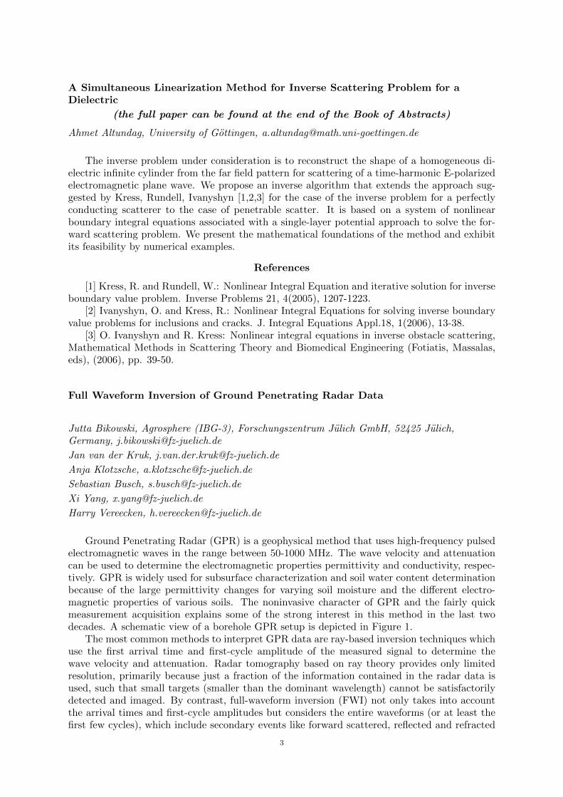
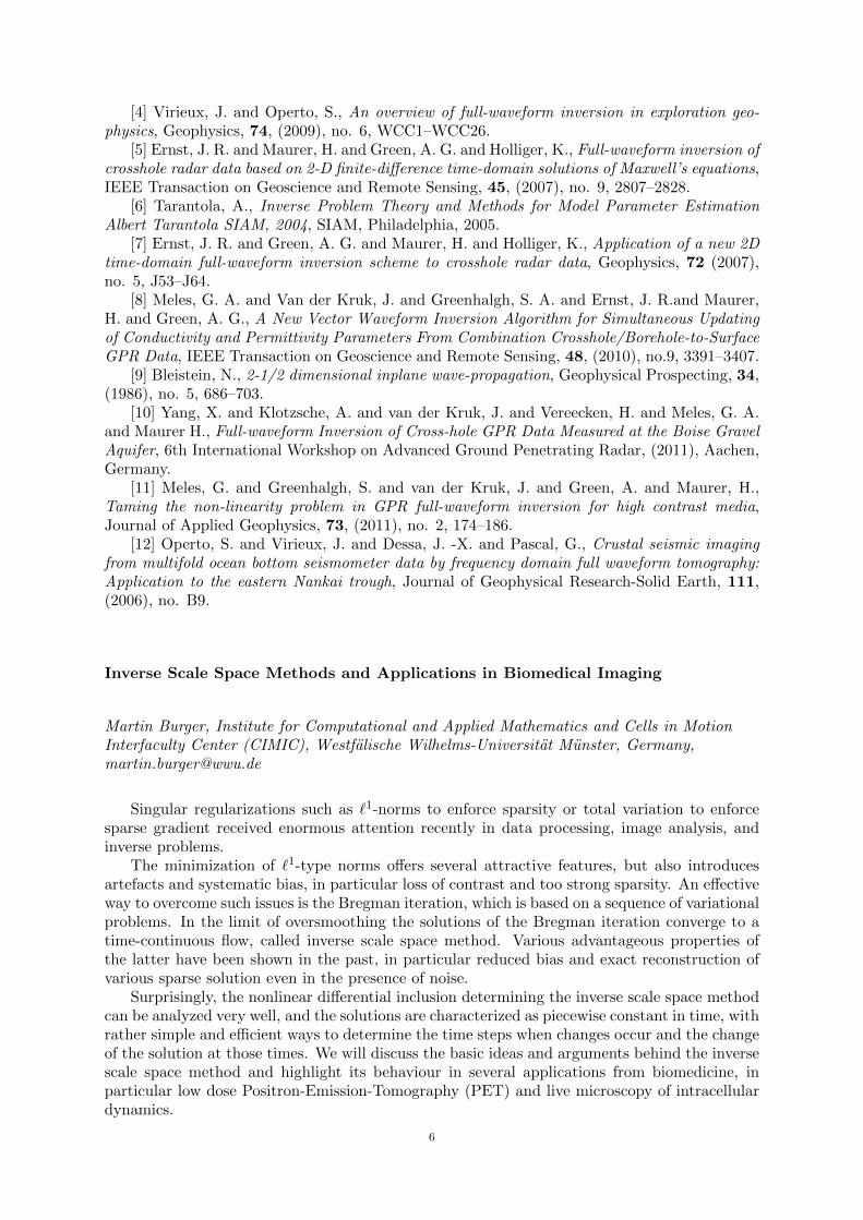
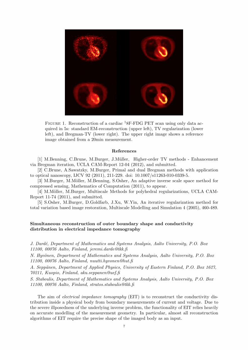
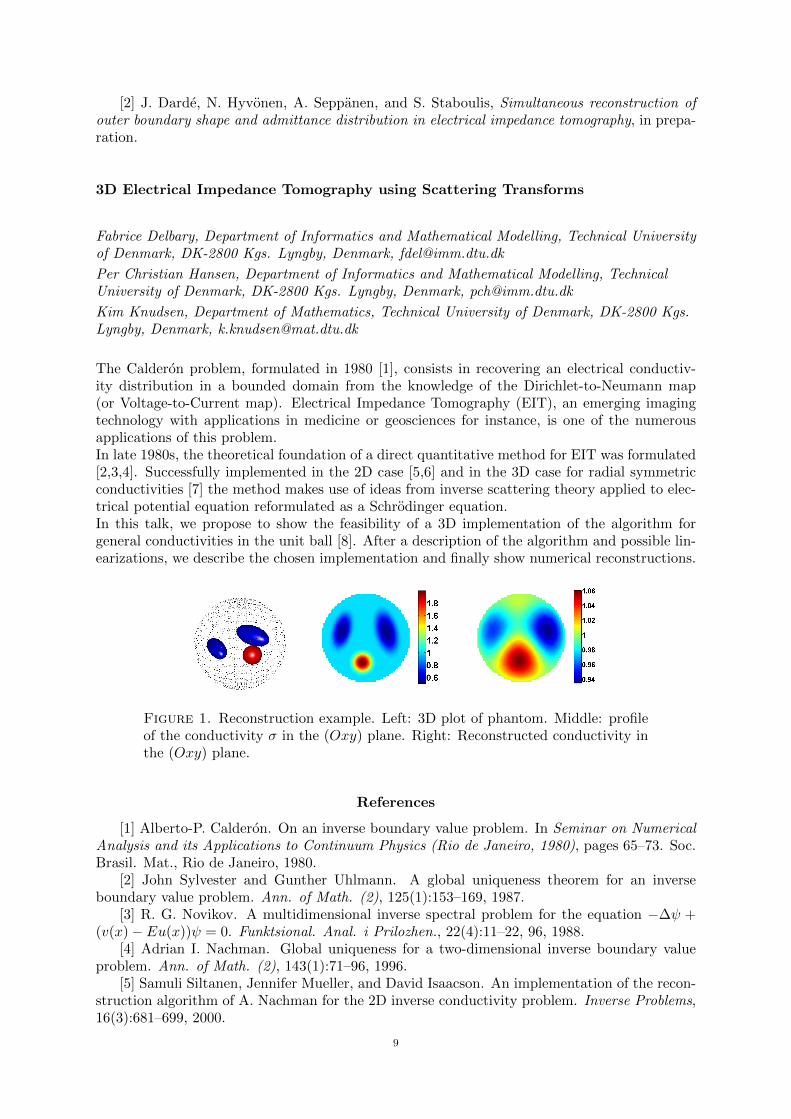
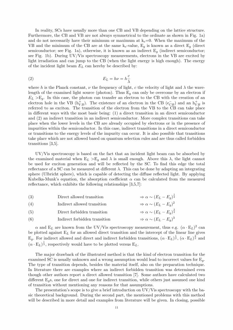

References
[1] B Harrach and J K Seo (2010) Exact shape-reconstruction by one-step linearizationin electrical impedance tomography SIAM J Math Anal 42 1505ndash1518
[2] B Harrach and M Ullrich (2010) Monotony based imaging in EIT AIP Conf Proc1281 1975ndash1978
Inverse Problems in Local Helioseismology
Thorsten Hohage Institut fur Numerische und Angewandte Mathematik 37083 GottingenGermany hohagemathuni-goettingende
Laurent Gizon Max Planck Institute for Solar System Research Max-Planck-Str 2 37191Katlenburg-Lindau Germany gizonmpsmpgde
The aim of local helioseismology is to compute three-dimensional reconstructions of flowvelocities and other physical quantities in the Solar interior from high resolution Doppler-shiftdata of the line-of-sight velocities
φ(r t) = l middot v(r t)
on the Sunrsquos surface Here l denotes the line of sight unit vector and v(r t) the velocity atposition r and time t Such data have been collected since 1995 by the ground based GlobalOscillations Network Group (GONG) and by the Michelson Doppler Imager (MDI) on boardof the Solar and Heliospheric Observatory (SOHO) launched 1995 In February 2010 the SolarDynamics Observatory (SDO) has been launched which collects more than 1TB of Doppler-shiftdata of the Sunrsquos surface velocity each day
Duvall et al [1] proposed to determine background flow velocities v0 in the convection zoneof the Sun by shifts of travel times of acoustic waves with respect to the standard Solar modelThey suggested to determine such travel time shifts using correlations of the form
C(r1 r2 t) =
int T
0φ(r1 t)φ(r2 t+ t) dt
The derivation of the corresponding forward problem can be summarized as follows (see [2]) Thedisplacements ξ(r t) of solar waves satisfy a wave equation L[v0]ξ = S in which the unknownbackground velocities v0 appear as parameters The sources S which are caused by turbulent
convection are modeled as a random process If (Oξ)(r t) = l middot parttξ(r z t) is defined such thatφ = OL[v0]minus1S then the covariance operators of S and φ are related by
Covφ[v0] = OL[v0]minus1CovSL[v0]minuslowastOlowast The covariance operator Covφ[v0] can be estimated by the integral operator
(Covφ[v0]w
)(r1 t) =
int intC(r1 r2 t2 minus t1)w(r2) dr2 dt2
Usually the signal-to-noise ratio of the point-to-point correlations C(r1 r2 t) is too small Inprinciple the signal-to-noise ratio can be made arbitrarily large by increasing the averaging timeT however T cannot be chosen too large to avoid motion blur To improve the signal-to-noiseratio and to reduce the length of the right hand side vector of the inverse problem certainspace-time averages of the form
τα(r1) =(
Covφ[v0]wα(middot minus r1))
(r1 0) =
int intC(r1 r1 + r2 t)wα(r2 t) dr2 dt
are computed The weights wα are chosen such that τα(r1) indicates some travel time of a wavestarting at r1 eg an average point-to-annulus travel time
16
We approximate Covφ[v0] asymp Covφ[0] + Covprimeφ[0]v0 by its first order Taylor approximationOn an approximately planar patch of the Sunrsquos surface there are sensitivity kernels Kαβ suchthat
((Covprimeφ[0]v0)wα(middot minus r1)
)(r1 0) =
sum
β
int int 0
minusz0Kαβ(r1 minus r2 z)v0β(r2 z) dr2 dz
Then the estimated travel time shifts δτα = τα minusCovφ[v0]wα(middot 0) satisfy the equation
(1) (δτα)(r1) =
int int 0
minusz0
sum
β
Kαβ(r1 minus r2 z)v0β(r2 z) dr2 dz + nα(r1)
The covariance kernelΛααprime(r2) = E [nα(r1)nαprime(r1 + r2)]
of the noise can be estimated from the case v0 = 0 (see [3])
The system of equations (1) is a linear statistical inverse problem
δτ = Kv0 + n
of a very nice structure After discretization of the z variable it has the form of a system ofconvolution equations where K is a matrix of two-dimensional convolution operators with thesensitivity kernels Kαβ as convolution kernels The covariance matrix of n is a full matrix butit is invariant with respect to horizontal translations and a good estimate is known A typicalsize of the problem is a 240 times 267 system of convolution operators on a grid of 4002 pointsresulting in about 4 middot 107 unknowns
Due to the assumed horizontal invariance it is possible to compute a complete singularvalue decomposition (SVD) of the forward operator since it separates into a system of smallSVDs for each spatial frequency We show how the physical side constraint div (ρv0) = 0 withthe density ρ = ρ(z) can be incorporated in the inversion procedure The special structureof the problem allows the use of Pinsker-type estimators which are known to be optimal forstatistical inverse problems among all linear estimators
We show some results for real data and compare our method to the method of Subtrac-tive Optimally Localized Averaging (SOLA) which can be seen as a version of the method ofapproximate inverse [4]
References
[1] T L Duvall Jr S M Jefferies J W Harvey and M A Pomerantz Time-distancehelioseismology Nature 362430ndash432 1993
[2] L Gizon and A C Birch Time-distance helioseismology The forward problem forrandom distributed sources The Astrophysical Journal 571(2)966 2002
[3] L Gizon and A C Birch Time-distance helioseismology Noise estimation The Astro-physical Journal 614(1)472 2004
[4] J Jackiewicz A C Birch L Gizon S Hanasoge T Hohage J B Ruffio and M SvandaMultichannel three-dimensional ola inversion for local helioseismology solar physics Solar Phys27619ndash33 2012
17
Conformal Mapping and Inverse Scattering
Rainer Kress Institut fur Numerische und Angewandte Mathematik Lotzestr 16-18 37083Gottingen Germany kressmathuni-goettingende
Akduman Haddar and Kress [124] have employed a conformal mapping technique for theinverse problem to recover a perfectly conducting or a nonconducting inclusion in a homogeneousbackground medium from Cauchy data on the accessible exterior boundary In a joint work [35]with Houssem Haddar Palaiseau France we proposed an extension of this approach to two-dimensional inverse electrical impedance tomography with piecewise constant conductivitiesA main ingredient of this method is the incorporation of the transmission condition on theunknown interior boundary via a nonlocal boundary condition in terms of an integral equation
More recently again together with Houssem Haddar we also proposed to use this conformalmapping approach to solve inverse scattering problems that is inverse boundary value problemsfor the Helmholtz equation for low frequencies via an iterative procedure We present thefoundations of this appraoch including a convergence result and exhibit the feasibility of themethod via numerical examples
References
[1] Akduman I and Kress R Electrostatic imaging via conformal mapping InverseProblems 18 1659ndash1672 (2002)
[2] Haddar H and Kress R Conformal mappings and inverse boundary value problemsInverse Problems 21 935ndash953 (2005)
[3] Haddar H and Kress R Conformal mapping and impedance tomography InverseProblems 26 074002 (2010)
[4] Kress R Inverse Dirichlet problem and conformal mapping Mathematics and Com-puters in Simulation 66 255ndash265 (2004)
[5] Kress R Inverse problems and conformal mapping Complex Variables and EllipticEquations 57 301ndash316 (2012)
Electrical impedance imaging using nonlinear Fourier transform
Samuli Siltanen University of Helsinki samulisiltanenikifi
The aim of electrical impedance tomography (EIT) is to reconstruct the inner structure of anunknown body from voltage-to-current measurements performed at the boundary of the bodyEIT has applications in medical imaging nondestructive testing underground prospecting andprocess monitoring The imaging task of EIT is nonlinear and an ill-posed inverse problemA non-iterative EIT imaging algorithm is presented based on the use of a nonlinear Fouriertransform Regularization of the method is provided by nonlinear low-pass filtering wherethe cutoff frequency is explicitly determined from the noise amplitude in the measured dataNumerical examples are presented suggesting that the method can be used for imaging theheart and lungs of a living patient
18
From KdV to NovikovndashVeselov and back
Andreas Stahel University of Applied Sciences Bern Quellgasse 21 CH-2501 BielSwitzerland AndreasStahelbfhch
Ryan Croke Department of Mathematics Colorado State University Fort Collins CO 80523USA crokemathcolostateedu
We present two numerical algorithms to solve the NovikovndashVeselov equations a 2+1 dimen-sional generalization of KdV We start with a numerical algorithm to solve the KdV equationThen verify that plane wave solutions to the NovikovndashVeselov equations are equivalent to solu-tions of KdV
KdV continuous and discrete conservation laws The Korteweg de Vries (KdV)equation is given by
(1) u(t x) = minusuprimeprimeprime(t x) + 6u(t x)uprime(t x)
has exact soliton solutions u(t x) = minusc2 cosh2(
radicc
2x)
This soliton solution has an amplitude of c2
and is traveling with speed c to the right It is an amazing fact that those soliton solutions canmove and pass by each other like solutions of linear problems But clearly the KdV equation (1)is a nonlinear initial value problem In Figure 1 find three solitons moving on an interval oflength 6 using periodic boundary conditions
Figure 1 KdV time evolution and contour levels for minusu(t x)
The nonlinear evolution problem (1) can be examined on an unbounded interval or on abounded interval with periodic boundary conditions Observe
bull If w(t x) is a solution of w(t x) = minuswprimeprimeprime(t x) ie the linear part of (1) then the L2
norm is conserved w(t middot)L2 = w(0 middot)L2 bull The L2 norm of the solution u(t x) of (1) is conserved
To develop efficient and reliable algorithm to generate numerical solutions to the KdV equationwe should respect the above
We examine (1) on a bounded space interval 0 le x le L with periodic boundary conditionsand use finite difference approximations for the differential expressions
bull For the third derivative we use a centered difference formula consistent of order 2This is represented by a matrix A including the periodic boundary conditions Theuprimeprimeprime(ti x) is approximated by A ~ui where ~ui represents the space discretization of thesolution u(ti x)
bull We use 6u(x)uprime(x) = 2(u2)prime
+2u(x)uprime(x) and use a matrix K computing the centeredfinite difference approximation of the first derivative Then the nonlinear contribution6u(ti x)uprime(ti x) is approximated by 2 K (~u(t) lowast ~u(t)) + 2 ~u(t) lowast (K ~u(t))
19
bull Now we use a standard CrankndashNicolson approximation for the time stepping fromti = i∆t to ti+1 = ti + ∆t The nonlinear contribution is approximated at themidpoint ~m = 1
2 (~ui + ~ui+1)
u(t x) = minusuprimeprimeprime(t x) + 6u(t x)uprime(t x)
~ui+1 minus ~ui∆t
= minus1
2A (~ui+1 + ~ui) + 2 (K (~m(t) lowast ~m(t)) + ~m(t) lowast (K ~m(t)))
For a given ~ui this is a system of nonlinear equations for ~ui+1bull If the nonlinear term is ignored (K = 0) we solve the linear problem u = minusuprimeprimeprime Since
the matrix A is skew-symmetric one can verify that the discrete solution does notchange the euclidean norm The verification is based on the midpoint vector ~m isorthogonal to the connecting vector ~w = 1
2 (~ui+1 minus ~ui) bull One may verify hat this nonlinear time stepping preserves the norm of the solutionbull Since the linearization of the above nonlinear term is easily written down we can use
Newtonrsquos method to solve the above problem
We obtain a fast stable numerical scheme to solve the KdV equation (1)
The NovikovndashVeselov Equations Numerical Solutions The NovikovndashVeselov equa-tion for function a q = q(t x y) on a two dimensional domain is given by
(2) q = minus1
4
part3
partx3q +
3
4
part3
partx party2q +
3
4div(q
(v1
v2
))
combined with the part equation
(3) partzv = partzq lArrrArr
partpartx v1 minus part
party v2 = + partpartx q
partpartx v2 + part
party v1 = minus partparty q
If we assume that the solution depends on x only we solve (3) by v1(x) = q(x) and v2 = 0and(2) simplifies to
q(t x) = minus1
4qprimeprimeprime(t x) +
3
4(q2(t x))prime
which is a KdV equationAnalytical and numerical problems for the NovikovndashVeselov equations are examined in the
forthcoming papers by Lassas Mueller Siltanen and Stahel ([12]) In this presentation wefocus on numerical aspects for the NovikovndashVeselov equations on a domain minusL le x y le L inR2
Dirichlet boundary conditions and the finite difference method We discretize the domain[minusLL] times [minusLL] by a uniform N times N grid with N2 points For each time level ti the spacediscretization of the solution q(ti x y) leads to a vector ~qi isin RNtimesN For the linear contributionsin (2) we use a leap-frog time stepping algorithm
1
4
part3
partx3q(ti x y)minus 3
4
part3
partx party2q(ti x y) minusrarr A
~qiminus1 + ~qi+1
2
linear part of equation (2) minusrarr ~qi+1 minus ~qiminus1
2 ∆t= minusA
~qiminus1 + ~qi+1
2
The N2 timesN2 matrix A is skew-symmetric and very sparse Thus approach leads to a conser-vation of the discrete L2 norm which coincides with the analytical behavior
By identifying the real vector (x y) isin R2 with z = x+ i y isin C we may then use the Greensfunction g(z) = 1
π z and the resulting formula for the solution of (3)
part v = f =rArr v(x y) =1
π
intint
R2
f(zprime)
z minus zprime dz
For a given function f this convolution integral is computed by FFT First a proper zero paddinghas to be applied ie the function f(z) is extended by 0 onto a larger domain For this to
work out nicely we need the function f(z) to vanish on the boundary resp the expressions part qpartx
20
and part qparty should be small To compute the approximation of div(q ~v) we use a finite difference
approximation for the gradient of q the apply the above convolution multiply by u and computethe divergence by finite difference again All of the above steps are represented by the nonlinearoperator M(~qi) Using a leap-frog scheme the NovikovndashVeselov equation (2) is replaced by
~qi+1 minus ~qiminus1
2 ∆t= minusA
~qiminus1 + ~qi+1
2+M(~qi)
(I + ∆tA)~qi+1 = (Iminus∆tA) ~qiminus1 + 2 ∆tM(~qi)(4)
For each time step the linear system (4) has to be solved With this algorithm we can solve theevolution problem (2) on large domains as shown in on the left in Figure 2
0
5
10
15
20
0
5
10
15
20
minus01
0
01
02
03
04
05
xy
Figure 2 Time evolution of the solution q(t x y) with Dirichlet (left) andperiodic (right) boundary conditions
Periodic boundary conditions and the spectral method If the NovikovndashVeselov equation (2)is solved with periodic boundary conditions we can use the previous finite difference methodor one can use a spectral method We work with a 2D Fourier approximation of the solutionThe Fourier solution q(t x y) on a square [0 L]times [0 L] is of the form
q(t x y) =Nminus1sum
jk=0
cjk(t) exp(i π
L(k x+ j y))
Translate (2) into a system of N2 nonlinear ordinary differential equations for the Fouriercoefficients cjk(t) We present an algorithm leading to the plane soliton solution on the rightin Figure 2
From planar solutions of NovikovndashVeselov to KdV We examine planar solution tothe NovikovndashVeselov equations (2) and (3) ie solution that depend only on one spatial variables = (n1 n2)middot(x y) only moving in a direction given by the vector ~n = (n1 n2) = (cos(α) sin(α))We seek solutions of the form q(t s) = q(t x y) = q(t n1 s n2 s) and verify that a planar solutionto (2) has to be a solution of the KdV-like equation
(5)4
κq(t s) = minusqprimeprimeprime(t s) + 6 q(t s) qprime(t s) +
3β
κqprime(t s)
where κ = cos(3α) and β is a constant For a solution u(t s) of KdV choose constants k1 and
k2 such that 3β4 = k1 + k2
3κ2 and verify that
q(t s) = u(κ
4t s+ k1 t)minus k2
is a solution of the NovikovndashVeselov equation This is a KdV solution observed in a movingframe with speed minusk1
21
References
[1] Matti Lassas Jennifer L Mueller Samuli Siltanen and Andreas Stahel The Novikov-Veselov equation and the Inverse Scattering Method part i Analysis Physica D NonlinearPhenomena 2012
[2] Matti Lassas Jennifer L Mueller Samuli Siltanen and Andreas Stahel The Novikov-Veselov equation and the Inverse Scattering Method part ii Computation Nonlinearity 2012
Optical characterisation of nanostructures using a discretised forward model
Mirza Karamehmedovic Foundation Institute of Materials Science (IWT) Department ofProduction Engineering University of Bremen Badgasteiner Str 3 28359 BremenGermany mirzaiwtuni-bremende
Mads Peter Soslashrensen Department of Mathematics Technical University of DenmarkDK-2800 Kgs Lyngby Denmark MPSoerensenmatdtudk
Poul-Erik Hansen Danish Fundamental Metrology Technical University of DenmarkDK-2800 Kgs Lyngby Denmark pehdfmdtudk
Andrei V Lavrinenko DTU Fotonik Technical University of Denmark DK-2800 KgsLyngby Denmark
Optical diffraction microscopy (ODM) is a non-destructive and relatively inexpensive meansof characterisation of nanostructures It is an essential tool in the design production andquality control of functional nanomaterials In ODM the target is reconstructed from themeasured optical power in the reflected far field This inverse scattering problem is typicallyhighly ill-posed due to the incompleteness of the data and the low signal-to-noise ratio In arealistic setting the formulation of the forward scattering model is usually complicated by thepresence of supporting structures (eg a substrate or a grid supporting a nanoparticle) sincethe electromagnetic interaction between the nanostructure and the supporting structure mustbe taken into account Also the roughness and the contamination of the supporting structurecan increase the dimensionality and the ill-posedness of the inverse problem Finally the size ofthe measured nanostructure is typically comparable to the wavelength of the illuminating lightso the scattering needs to be described using the full Maxwellian electromagnetic model ratherthan (numerically inexpensive) asymptotic formulations
We here describe an efficient accurate and robust forward scattering model [12] based ondiscrete sources and tailor-made for the reconstruction of 2D nanoparticles on substrates fromODM data We adopt an analysis-based modelling paradigm and attempt to incorporate asmuch available a priori information as possible directly in the forward model We replacethe classical radiation integrals by finite linear combinations of stratified Greenrsquos functions forthe Helmholtz operator in the plane and thus achieve a sparse formulation and an implicitdescription of the particle-substrate interaction The forward model can be extended to includethe roughness and contamination of the substrate without sacrificing the speed of computation[3] We validate the model and show its feasibility in a decomposition-type inverse schemewith synthetic measurement data ([1] figure 1) as well as in the inversion of experimentalscatterometric data ([4] figure 2) Finally we use a related forward model in the inversion ofsynthetic measurement data to estimate aperiodic defects in a nanograting ([5] figure 3)
References
[1] M Karamehmedovic P-E Hansen and T Wriedt A fast inversion method for highlyconductive submicron wires on a substrate Journal of the European Optical Society ndash RapidPublications 6(11039) 2011
22
Figure 1 Cross-section reconstruction for a highly conductive nanowire on asmooth Si substrate using synthetic data The forward model uses discretesources Bottom the reconstructed near-field amplitude (left) and phase (right)
[2] M Karamehmedovic P-E Hansen and T Wriedt An efficient scattering model forPEC and penetrable nanowires on a dielectric substrate Journal of the European Optical Societyndash Rapid Publications 6(11021) 2011
[3] M Karamehmedovic P-E Hansen and T Wriedt An efficient rough-interface scat-tering model for embedded nanostructures Thin Solid Films DOI 101016jtsf2012110482012
[4] M Karamehmedovic P-E Hansen K Dirscherl E Karamehmedovic and T WriedtProfile estimation for Pt submicron wire on rough Si substrate from experimental data OpticsExpress 20(19) 21678ndash21686 2012
[5] M Karamehmedovic M P Soslashrensen P-E Hansen and A V Lavrinenko Applicationof the method of auxiliary sources to a defect-detection inverse problem of optical diffractionmicroscopy Journal of the European Optical Society ndash Rapid Publications 5(10021) 2010
23
Figure 2 Cross-section reconstruction for a Pt nanowire on a rough contam-inated Si substrate using experimental ODM data The forward model usesdiscrete sources Top SEM and AFM images of the nanowire Bottom theforward scattering model and the reconstructed near-field amplitude
Figure 3 Left a nanograting defect to be characterised by ODM with thediscrete sources forward model Right a FEM computation of the amplitude ofthe scattered near field for the defect-free scatterer
24
A SECOND DEGREE NEWTONrsquoS METHOD IN INVERSE SCATTERING
PROBLEM
RAINER KRESS AND KUO-MING LEE
The inverse problem of recovering the geometry and the physical properties of a scatterer from theknowledge of the far field pattern of the scattered field is of fundamental importance for example innon-destructive testing seismic research or medical imaging In this talk we consider as a model thetime-harmonic scattering problem from a sound-soft obstacle The aim of our inverse problem is torecover the unknown scatterer from the knowledge of the far field pattern
Based on integral equation the scattering problem can be formulated in the following operator form
(01) F (Γ) = uinfin
Indeed for the direct problem this equation gives the far field pattern uinfin from the knowledge of theboundary Γ of the obstacle with a given incident wave For the inverse problem one would like to findthe unknown boundary Γ from the (measured) far field data by solving this so-called far field equation(01) As opposed to the direct problem which is linear and well-posed in the sense of Hadamard theinverse problem is nonlinear and ill-posed Hence both linearization and regularization are needed at thesame time Because of its conceptual simplicity and accuracy of the reconstruction Newtonrsquos method is agood candidate for the linearization of the inverse problem The familiar Newtonrsquos method approximatesthe nonlinear operator via a linear one which is just the first derivative of the original one Here byreplacing the linear approximation of the nonlinear operator with a second degree approximation wewant to investigate whether the numerical performance can be improved Furthermore our second degreemethod can be carried out via two consecutive linear steps This is advantageous in the sense that thewhole inverse scheme remains in the setting of linear regularization theory
References
[1] R Kress and K-M Lee A second degree Newton method for an inverse obstacle scattering problem Journal ofComputational Physics 20 (2011) 761ndash769
Institut fur Numerische und Angewandte Mathematik University of Gottingen 37083 Gottingen Germany
E-mail address kressmathuni-goettingende
Department of Mathematics National Cheng Kung University701 Tainan Taiwan
E-mail address kmleemailnckuedutw
WORKSHOP bdquoINVERSE PROBLEMS AND NUMERICAL METHODS IN APPLICATIONSldquo
Title of presentation Determination of Heat Transfer Coefficients from cooling curves ndash an inverse problem of heat conduction Author
Thomas Luumlbben Affiliation
Stiftung Institut fuumlr Werkstofftechnik IWT Division Materials Science Department Heat treatment Badgasteiner Str 3 Germany luebbeniwt-bremende
Abstract One of the most important processes in heat treatment is the hardening process Aim of it is the increase of hardness (mechanical resistance against a mechanical penetration of a harder test body) and strength (maximum stress until cracking) To do this for steels the component has to be heated to a steel specific temperature During this process the steel will undergo a phase transformation The cubic body centered lattice will change to the cubic face centered one (called austenite) Furthermore carbides will be dissolved and the carbon will be distributed homogeneously by diffusion processes in the component This is possible because the austenite can assimilate much more carbon than the ferritic phases with cbc lattice In the second step the component has to be cooled with an overcritical steel depending cooling rate to avoid that the carbon atoms leave their position by diffusion and to achieve the phase martensite with a significant increase of hardness and strength This cooling process is called quenching and two research groups at IWT are working on this topic The group ldquoMultiphase Flow Heat- and Mass-Transferrdquo of Udo Fritsching (division ldquoProcess amp Chemical Engineering) is dealing with modeling and simulation of multiphase flowing systems by Computational Fluid Dynamics (CFD) The group of Thomas Luumlbben works on heat treatment simulation and needs the Heat Transfer Coefficient (HTC) as boundary condition to the solution of the heat conduction equation (material properties are temperature and phase dependent)
Q)grad(divt
cp +θsdotλ=partθpart
sdotsdotρ (1)
ρ [kgmsup3] density of the steel (temperature and phase dependent) cp [J(kgK)] specific heat capacity of the steel (temperature and phase dependent) λ [W(mK)] heat conductivity of the steel (temperature and phase dependent) Q [Wmsup3] intensity of internal heat sources (in general time dependent) θ [degC] temperature t [s] time For quenching media which exhibit only convective heat transfer as gases molten salts or water with a very high velocity (in the order of 10 ms) the HTC calculated by CFD can be used for heat treatment simulation CFD delivers the HTC for the complete surface of a component and if necessary even the corresponding time dependencies But in general a calibration of the model has to be done by a HTC
measurement Equation (1) can be simplified if no axial und circumferential heat flux occurs For a cylindrical body without phase transformations equation (2) results
θ (2) r [m] coordinate in radial direction By measuring the temperature near to the surface in the middle plane of the cylinder the inverse heat conduction problem for this simple case can be solved by optimization methods or by an inverse calculation by use of Dirichlet-condition For quenching media with a boiling temperature lower than the start temperature of the austenitized components (water and special oils) the heat transfer is much more complicated Two phases of the fluid have to be taken into account the liquid and the vapor of this liquid Instead of one mechanism two additional ones have to be considered film boiling and nucleate boiling A typical local temperature dependency of the HTC of a quenching oil is shown in the left figure
HTC as function of surface temperature (left) and
typical behavior of rewetting (right FP film boiling KP nucleate boiling Kon convection) After immersion of the component into the quenching media a prompt evaporation of the oil directly at the surface occur and vapor film is formed around the component This film acts as isolator and the resulting HTC is quite small After some time the vapor film breaks down at the lower edge of the cylinder and nucleate boiling starts (right figure) As a result of the direct contact between fluid and surface the HTC increases dramatically The front between film and nucleate boiling moves (rewetting) and after the local temperature drops below the boiling temperature convection starts In some cases a second front starts at the upper edge In consequence a complicated distribution of the HTC results with axial and in general circumferential heat fluxes Therefore the assumptions described above are not fulfilled and equation (2) cannot be used under these conditions But with special equipment circumferential heat fluxes can be avoided Than by use of
θ λ (3) z [m] coordinate in axial direction the problem has to be solved Again optimization methods can be used But investigations from literature show that the evaluation time for the method which provides acceptable results is comparable high (74 hours) For this reason a cooperation with the ldquoZentrum fuumlr Technomathematikrdquo (ZeTem) at the University of Bremen was started Within the frame of a modeling seminar two students started with the development of software tools for the estimation of the HTC as function of temperature and position In the lecture some results were presented and resulting problems discussed
A SIMULTANEOUS LINEARIZATION METHOD FOR INVERSE
SCATTERING PROBLEM FOR A DIELECTRIC
AHMET ALTUNDAG
Abstract The inverse problem under consideration is to reconstruct the shape of a homo-
geneous dielectric infinite cylinder from the far field pattern for scattering of a time-harmonic
E-polarized electromagnetic plane wave We propose an inverse algorithm that extends the ap-proach suggested by Kress and Rundell [13] and further investigated by Ivanyshyn and Kress
[5 6] for the case of the inverse problem for a perfectly conducting scatterer to the case of
penetrable scatter It is based on a system of nonlinear boundary integral equations associatedwith a single-layer potential approach to solve the forward scattering problem We present the
mathematical foundations of the method and exhibit its feasibility by numerical examples
1 Introduction
In inverse obstacle scattering problems for time-harmonic waves the scattering object is a ho-mogeneous obstacle and the inverse problem is to obtain an image of the scattering object iean image of the shape of the obstacle from a knowledge of the scattered wave at large distancesie from the far field pattern In the current paper we deal with dielectric scatterers and confineourselves to the case of infinitely long cylinders
Assume that the simply connected bounded domain D sub IR2 with C2 boundary partD representsthe cross section of a dielectric infinite cylinder having constant wave number kd with Re kd gt 0and Im kd ge 0 embedded in a homogeneous background with positive wave number k0 Denote byν the outward unit normal to partD Then given an incident plane wave ui(x) = eik0 xmiddotd with incidentdirection given by the unit vector d the direct scattering problem for Endashpolarized electromagneticwaves is modeled by the following transmission problem for the Helmholtz equation Find solutionsu isin H1
loc(IR2 D) and v isin H1(D) to the Helmholtz equations
(11) 4u+ k20u = 0 in IR2 D 4v + k2dv = 0 in D
satisfying the transmission conditions
(12) u = vpartu
partν=partv
partνon partD
in the trace sense such that u = ui + us with the scattered wave us fulfilling the Sommerfeldradiation condition
(13) limrrarrinfin
r12(partus
partrminus ik0us
)= 0 r = |x|
uniformly with respect to all directions The latter is equivalent to an asymptotic behavior of theform
(14) us(x) =eik0|x|radic|x|
uinfin
(x
|x|
)+O
(1
|x|
) |x| rarr infin
Key words and phrases inverse scattering Helmholtz equation transmission problem singlelayer approachnonlinear integral equations iterative methods
1
2A SIMULTANEOUS LINEARIZATION METHOD FOR INVERSE SCATTERING PROBLEM FOR A DIELECTRIC
uniformly in all directions with the far field pattern uinfin defined on the unit circle S1 in IR2
(see[4]) In the above u and v represent the electric field that is parallel to the cylinder axis (11)corresponds to the time-harmonic Maxwell equations and the transmission conditions (12) modelthe continuity of the tangential components of the electric and magnetic field across the interfacepartD
The inverse obstacle problem we are interested in is given the far field pattern uinfin for oneincident plane wave with incident direction d isin S1 to determine the boundary partD of the scatteringdielectric D More generally we also consider the reconstruction of partD from the far field patternsfor a small finite number of incident plane waves with different incident directions This inverseproblem is nonlinear and ill-posed since the solution of the scattering problem (11)ndash(13) is non-linear with respect to the boundary and since the mapping from the boundary into the far fieldpattern is extremely smoothing
At this point we note that uniqueness results for this inverse transmission problem are onlyavailable for the case of infinitely many incident waves (see [9]) A general uniqueness result basedon the far field pattern for one or finitely many incident waves is still lacking More recently auniqueness result for recovering a dielectric disk from the far field pattern for scattering of oneincident plane wave was established by Altundag and Kress [2]
In the spirit of the approach for scattering from a perfect conductor proposed by Kress andRundell [15] in electrostatics and further investigated by Ivanyshyn and Kress [7] in electromag-netics
For a stable solution of the inverse transmission problem we propose an algorithm that extendsthe approach suggested by Kress and Rundell [13] in electromagnetics and further investigatedby Kress and Ivanyshyn [5 6] for the case of the inverse problem for a perfectly conductingscatterer Representing the solution v and us to the forward scattering problem in terms of single-layer potentials in D and in IR2 D with densities ϕd and ϕ0 respectively the transmissioncondition (12) provides a system of two boundary integral equations on partD for the correspondingdensities that in the sequel we will denote as field equations For the inverse problem the requiredcoincidence of the far field of the single-layer potential representing us and the given far field uinfinprovides a further equation that we denote as data equation The system of the field and dataequations can be viewed as three equations for three unknowns ie the two densities and theboundary curve They are linear with respect to the densities and nonlinear with respect to theboundary curve
In the spirit of [5 6 13] given an approximation partDapprox for the boundary partD and approxi-mations ϕdapprox and ϕ0approx for the densities ϕd and ϕ0 we linearize both the field and the dataequations simultaneously with respect to the boundary curve and the two densities The linearequations are then solved to update both the boundary curve and the two densities Because of theill-posedness the solution of the update equations require stabilization for example by Tikhonovregularization This procedure is then iterated until some suitable stopping criterion is satisfied
The plan of the paper is as follows In Section 2 as ingredient of our inverse algorithm wedescribe the solution of the forward scattering problem via a single-layer approach followed by acorresponding numerical solution method in Section 3 The details of the inverse algorithm arepresented in Section 4 and in Section 5 we demonstrate the feasibility of the method by somenumerical examples
2 The direct problem
The forward scattering problem (11)ndash(13) has at most one solution (see [3 12] for the three-dimensional case) Existence can be proven via boundary integral equations by a combined single-and double-layer approach (see [3 12] for the three-dimensional case) Here we base the solution
A SIMULTANEOUS LINEARIZATION METHOD FOR INVERSE SCATTERING PROBLEM FOR A DIELECTRIC3
of the forward problem on a single-layer approach as investigated in [2] For this we denote by
Φk(x y) =i
4H
(1)0 (k|xminus y|) x 6= y
the fundamental solution to the the Helmholtz equation with wave number k in IR2 in terms of the
Hankel function H(1)0 of order zero and of the first kind Adopting the notation of [4] in a Sobolev
space setting for k = kd and k = k0 we introduce the single-layer potential operators
Sk Hminus12(partD)rarr H12(partD)
by
(25) (Skϕ)(x) = 2
int
partD
Φk(x y)ϕ(y) ds(y) x isin partD
and the normal derivative operators
K primek Hminus12(partD)rarr Hminus12(partD)
by
(26) (K primekϕ)(x) = 2
int
partD
partΦk(x y)
partν(x)ϕ(y) ds(y) x isin partD
For the Sobolev spaces and the mapping properties of these operators we refer to [11 17]Then from the jump relations it can be seen that the single-layer potentials
(27)
v(x) =
int
partD
Φkd(x y)ϕd(y) ds(y) x isin D
us(x) =
int
partD
Φk0(x y)ϕ0(y) ds(y) x isin IR2 D
solve the scattering problem (11)ndash(13) provided the densities ϕd and ϕ0 satisfy the system ofintegral equations
(28)
Skdϕd minus Sk0ϕ0 = 2ui|partD
ϕd +K primekdϕd + ϕ0 minusK primek0ϕ0 = 2partui
partν
∣∣∣∣partD
which in the squel we will call the field equations Provided k0 is not a Dirichlet eigenvalue of thenegative Laplacian for the domain D with the aid of the Riesz-Fredholm theory in [2] it has beenshown that the system (28) has a unique solution in Hminus12(partD)timesHminus12(partD) Thus throughoutthis paper we shall assume that k0 is not a Dirichlet eigenvalue of the negative Laplacian for thedomain D
After introducing the far field operator Sinfin Hminus12(partD)rarr L2(S1) by
(29) (Sinfinϕ)(x) = γ
int
partD
eminusik0 xmiddotyϕ(y) ds(y) x isin S1
from (27) and asymptotics of the Hankel function we observe that the far field pattern for thesolution to the scattering problem (11)ndash(13) is given by
(210) uinfin = Sinfinϕ0
in terms of the solution to (28)
4A SIMULTANEOUS LINEARIZATION METHOD FOR INVERSE SCATTERING PROBLEM FOR A DIELECTRIC
3 Numerical solution
For the numerical solution of (28) and the presentation of our inverse algorithm we assume thatthe boundary curve partD is given by a regular 2πndashperiodic parameterization
(31) partD = z(t) 0 le t le 2π
Then via ψ = ϕ z emphasizing the dependence of the operators on the boundary curve weintroduce the parameterized single-layer operator
Sk Hminus12[0 2π]times C2[0 2π]rarr H12[0 2π]
by
Sk(ψ z)(t) =i
2
int 2π
0
H(1)0 (k|z(t)minus z(τ)|) |zprime(τ)|ψ(τ) dτ
and the parameterized normal derivative operators
K primek Hminus12[0 2π]times C2[0 2π]rarr Hminus12[0 2π]
by
K primek(ψ z)(t) =ik
2
int 2π
0
[zprime(t)]perp middot [z(τ)minus z(t)]|zprime(t)| |z(t)minus z(τ)| H
(1)1 (k|z(t)minus z(τ)|) |zprime(τ)|ψ(τ) dτ
for t isin [0 2π] Here we made use of H(1)prime0 = minusH(1)
1 with the Hankel function H(1)1 of order zero
and of the first kind Furthermore we write aperp = (a2minusa1) for any vector a = (a1 a2) that is aperp
is obtained by rotating a clockwise by 90 degrees Then the parameterized form of (28) is givenby
(32)
Skd(ψd z)minus Sk0(ψ0 z) = 2ui z
ψd + K primekd(ψd z) + ψ0 minus K primek0(ψ0 z) =2
|zprime| [zprime]perp middot gradui z
The kernels
M(t τ) =i
2H
(1)0 (k|z(t)minus z(τ)|) |zprime(τ)|
and
L(t τ) =ik
2
[zprime(t)]perp middot [z(τ)minus z(t)]|zprime(t)| |z(t)minus z(τ)| H
(1)1 (k|z(t)minus z(τ)|) |zprime(τ)|
of the operators Sk and K primek can be written in the form
(33)
M(t τ) = M1(t τ) ln
(4 sin2 tminus τ
2
)+M2(t τ)
L(t τ) = L1(t τ) ln
(4 sin2 tminus τ
2
)+ L2(t τ)
A SIMULTANEOUS LINEARIZATION METHOD FOR INVERSE SCATTERING PROBLEM FOR A DIELECTRIC5
where
M1(t τ) = minus 1
2πJ0(k|z(t)minus z(τ)|)|zprime(τ)|
M2(t τ) = M(t τ)minusM1(t τ) ln
(4 sin2 tminus τ
2
)
L1(t τ) = minus k
2π
[zprime(t)]perp middot [z(τ)minus z(t)]|zprime(t)| |z(t)minus z(τ)| J1(k|z(t)minus z(τ)|) |zprime(τ)|
L2(t τ) = L(t τ)minus L1(t τ) ln
(4 sin2 tminus τ
2
)
The functions M1M2 L1 and L2 turn out to be smooth with diagonal terms
M2(t t) =
[i
2minus C
πminus 1
πln
(k
2|zprime(t)|
)]|zprime(t)|
in terms of Eulerrsquos constant C and
L2(t t) = minus 1
2π
[zprime(t)]perp middot zprimeprime(t)|zprime1(t)|2
For integral equations with kernels of the form (33) a combined collocation and quadrature meth-ods based on trigonometric interpolation as described in Section 35 of [4] or in [16] is at ourdisposal We refrain from repeating the details For a related error analysis we refer to [11] andnote that we have exponential convergence for smooth ie analytic boundary curves partD
For a numerical example we consider the scattering of a plane wave by a dielectric cylinder with anon-convex kite-shaped cross section with boundary partD described by the parametric representation
(34) z(t) = (cos t+ 065 cos 2tminus 065 15 sin t) 0 le t le 2π
From the asymptotics for the Hankel functions it can be deduced that the far field pattern ofthe single-layer potential us with density ϕ0 is given by
(35) uinfin(x) = γ
int
partD
eminusik0 xmiddotyϕ0(y) ds(y) x isin S1
where
γ =eiπ4radic
8πk0
The latter expression can be evaluated by the composite trapezoidal rule after solving the systemof integral equations (28) for ϕ0 ie after solving (32) for ψ0 Table 31 gives some approximatevalues for the far field pattern uinfin(d) and uinfin(minusd) in the forward direction d and the backwarddirection minusd The direction d of the incident wave is d = (1 0) and the wave numbers are k0 = 1and kd = 2 + 3i Note that the exponential convergence is clearly exhibited
6A SIMULTANEOUS LINEARIZATION METHOD FOR INVERSE SCATTERING PROBLEM FOR A DIELECTRIC
Table 31 Numerical results for direct scattering problem
n Reuinfin(d) Imuinfin(d) Reuinfin(minusd) Imuinfin(minusd)
8 -06017247940 -00053550779 -02460323014 0318495776816 -06018967551 -00056192337 -02461831740 0318605268632 -06019018135 -00056277492 -02461946976 0318604994964 -06019018076 -00056277397 -02461946846 03186049951
4 The inverse problem
We now proceed describing an iterative algorithm for approximately solving the inverse scatter-ing problem by extending the method proposed by Kress [13] and further investigated by Ivanyshynand Kress [5 6] for the case of the inverse problem for a perfectly conducting scatterer to the caseof a dielectric scatterer
After introducing the far field operator Sinfin Hminus12(partD)rarr L2(S1) by
(41) (Sinfinϕ)(x) = γ
int
partD
eminusik0 xmiddotyϕ(y) ds(y) x isin S1
from (27) and (35) we observe that the far field pattern for the solution to the scattering problem(11)ndash(13) is given by
(42) uinfin = Sinfinϕ0
in terms of the solution to (28)
41 The inverse problem for shape reconstruction We can state the following theorem astheoretical basis of our inverse algorithm For this we note that all our integral operators dependon the boundary curve partD
Theorem 41 For a given incident field ui and a given far field pattern uinfin assume that partD andthe densities ϕd and ϕ0 satisfy the system of three integral equations
(43)
Skdϕd minus Sk0ϕ0 = 2ui
ϕd +K primekdϕd + ϕ0 minusK primek0ϕ0 = 2partui
partν
Sinfinϕ0 = uinfin
Then partD solves the inverse problem
The ill-posedness of the inverse problem is reflected through the ill-posedness of the third integralequation the far field equation that we denote as data equation Note that (43) is linear withrespect to the densities and nonlinear with respect to the boundary partD This opens up a varietyof approaches to solve (43) by linearization and iteration In [2] we investigated an extensionof the approach suggested by Johansson and Sleeman [8] for a perfectly conducting scattererGiven a current approximation partDapprox for the unknown boundary partD we first solved the firsttwo equations or field equations of system (43) for the unknown densities ϕd and ϕ0 Thenkeeping ϕ0 fixed we linearized the third equation or data equation of system (43) with respectto the boundary partD to update the approximation Here following [5 6 13] we are going toproceed differently given an approximation partDapprox for the boundary partD and approximationsϕdapprox and ϕ0approx for the densities ϕd and ϕ0 we linearize both the field and the data equationssimultaneously with respect to the boundary curve and the two densities The linear equations are
A SIMULTANEOUS LINEARIZATION METHOD FOR INVERSE SCATTERING PROBLEM FOR A DIELECTRIC7
then solved to update both the boundary curve and the two densities Because of the ill-posednessthe solution of the update equations require stabilization for example by Tikhonov regularizationThis procedure is then iterated until some suitable stopping criterion is satisfied
To describe this in more detail we also require the parameterized version
Sinfin Hminus12[0 2π]times C2[0 2π]rarr L2(S1)
of the far field operator as given by
(44) Sinfin(ψ z)(x) = γ
int 2π
0
eminusik0 xmiddotz(τ)ψ(τ) dτ x isin S1
Then the parameterized form of (43) is given by
(45)
Skd(ψd z)minus Sk0(ψ0 z) = 2ui z
ψd + K primekd(ψd z) + ψ0 minus K primek0(ψ0 z) =2
|zprime| [zprime]perp middot gradui z
Sinfin(ψ0 z) = uinfin
For a fixed ψ the Frechet derivative of the operator Sk and K primek with respect to the boundary zin the direction h are given by (see [18])
Sprimek(ψ zh)(t) =minusik
2
int 2π
0
(z(t)minus z(τ)) middot (h(t)minus h(τ))
|z(t)minus z(τ)| |zprime(τ)|H(1)1 (k|z(t)minus z(τ)|)ψ(τ)dτ
+i
2
int 2π
0
zprime(τ) middot hprime(τ)
|zprime(τ)| H(1)0 (k|z(t)minus z(τ)|)ψ(τ)dτ(46)
and(47)
(K primek)prime(ψ zh)(t) =
minus ik
2|zprime(t)|int 2π
0
[zprime(t)]perpmiddot(h(t)minush(τ))+[hprime(t)]perpmiddot(z(t)minusz(τ))
|z(t)minusz(τ)| |zprime(τ)|H(1)1 (k|z(t)minusz(τ)|)ψ(τ)dτ
+ik
|zprime(t)|
int 2π
0
[zprime(t)]perpmiddot(z(t)minusz(τ))(h(t)minush(τ))middot(z(t)minusz(τ))
|z(t)minusz(τ)|3 |zprime(τ)|H(1)1 (k|z(t)minusz(τ)|)ψ(τ)dτ
minus ik2
2|zprime(t)|
int 2π
0
[zprime(t)]perpmiddot(z(t)minusz(τ))(h(t)minush(τ))middot(z(t)minusz(τ))
|z(t)minusz(τ)|2 |zprime(τ)|H(1)0 (k|z(t)minusz(τ)|)ψ(τ)dτ
+ik
2
hprime(t) middotzprime(t)|zprime(t)|2
int 2π
0
[zprime(t)]perp middot(z(t)minusz(τ))
|z(t)minus z(τ)| |zprime(τ)|H(1)1 (k|z(t)minusz(τ)|)ψ(τ)dτ
minus ik
2|zprime(t)|
int 2π
0
[zprime(t)]perp middot(z(t)minusz(τ))hprime(τ)middotzprime(τ)
|z(t)minusz(τ)||zprime(τ)| H(1)1 (k|z(t)minusz(τ)|)ψ(τ)dτ
8A SIMULTANEOUS LINEARIZATION METHOD FOR INVERSE SCATTERING PROBLEM FOR A DIELECTRIC
Then the linearization (45) with respect to all variables z ϕd and ϕ0 in the direction h ηd andη0 respectively reads
(48)
Skd(ψd z) + Skd(ηd z) + Sprimekd(ψd zh)minus Sk0(ψ0 z)minus Sk0(η0 z)
minusSprimek0(ψ0 zh) = 2ui z + 2gradui z middot h
ψd + ηd + ψ0 + η0 + K primekd(ψd z) + K primekd(ηd z) + (K primed)prime(ψd zh)
minusK primek0(ψ0 z)minus K primek0(η0 z)minus (K primek0)prime(ψ0 zh) =2
|zprime| [zprime]perp middot gradui z + 2ξ(z) middot h
Sinfin(ψ0 z) + Sinfin(η0 z) + Sprimeinfin(ψ0 zh) = uinfin
Here the term ξ(z) middot h is the form ( see [19 20])
(49) ξ(z) middot h = minuspartui
partτ
ν middot hprime|zprime| + (
part2ui
partνpartτminusHpartui
partτ)τ middot h+
part2ui
partν2ν middot h
and τ and H stand for the tangential vector and the mean curvature respectively They are givenby
τ =zprime
|zprime| and H = minuszprimeprime middot ν|zprime|2
and the matrix form of (48) can be written as
(410)
Sprimekd(ψd z middot)minus Sprimek0(ψ0 z middot)minus 2gradui z Skd(middot z) minusSk0(middot z)
(K primekd)prime(ψd z middot)minus (K primek0)prime(ψ0 z middot)minus 2ξ(z) I + K primekd(middot z) I minus K primek0(middot z)
Sprimeinfin(ψ0 z middot) 0 Sinfin(middot z)
h
ηd
η0
=
2ui z minus Skd(ψd z) + Sk0(ψ0 z)
2
|zprime| [zprime]perp middot gradui z minus ψd minus K primekd(ψd z)minus ψ0 + K primek0(ψ0 z)
uinfin minus Sinfin(ψ0 z)
Now we can describe the method in a short form as follows
Each iteration step of the proposed inverse algorithm consists of one part
bull Given an approximation z for the boundary and densities ψd ψ0 we solve the linearizedsistem of integral equations (410) for h ηd and η0 to obtain updates z + h ψd + ηd andψ0 +η0 We continue this procedure until some stopping criteria is achieved The stoppingcriterion for the iterative scheme is given by the relative error
(411) uinfinN minus uinfin uinfin
le ε
where uinfinN is the computed far field pattern after N iteration steps
A SIMULTANEOUS LINEARIZATION METHOD FOR INVERSE SCATTERING PROBLEM FOR A DIELECTRIC9
Here we note that only in the first iteration step it is convenient to start from an approximationz for the boundary and solve the first two equations in (45) for the densities
Because of the ill-posedness the solution of (410) requires stabilization for instance by Tikhonovregularization We choose for the boundary Hp penalty term and the regularization parameterλ = (08)j decreasing with the iteration step j and for the densities L2 penalty term and theregularization parameter α = 10minus6
In principle the parameterization of the update is not unique To cope with this ambiguityone possibility that we will pursue in our numerical examples of the subsequent section is to allowonly parameterizations of the form
(412) z(t) = r(t)
(cos tsin t
) 0 le t le 2π
with a non-negative function r representing the radial distance of partD from the origin Consequentlythe perturbations are of the form
(413) h(t) = q(t)
(cos tsin t
) 0 le t le 2π
with a real function q In the approximations we assume r and its update q to have the form of atrigonometric polynomial of degree J in particular
(414) q(t) =
Jsum
j=0
aj cos jt+
Jsum
j=1
bj sin jt
Then the update equation (410) is solved in the least squares sense penalized via Tikhonov reg-ularization for the unknown coefficients a0 aJ and b1 bJ of the trigonometric polynomialrepresenting the update q As experienced in the application of the above approach for relatedproblems it is advantageous to use an Hp Sobolev penalty term rather than an L2 penalty in the
Tikhonov regularization ie to interpret Sprimek and (K primek)prime as ill-posed linear operators
(415) Sprimek Hp[0 2π]rarr L2[0 2π] (K primek)prime Hp[0 2π]rarr L2[0 2π]
for some small p isin INAs a theoretical basis for the application of Tikhonov regularization from [4] we cite that after
the restriction to star-like boundaries the operator Sprimek and (K primek)prime are injective provided k2 is nota Neumann eigenvalue for the negative Laplacian in D
The above algorithm has an extension for the case of more than one incident wave Assumethat ui1 u
iM are M incident waves with different incident directions and uinfin1 uinfinM the
corresponding far field patterns for scattering from partD Then the inverse problem to determinethe unknown boundary partD from these given far field patterns and incident fields is equivalent tosolve the following equation for the boundary z and densities ψd1 ψdM and ψ01 ψ0M
(416)
Skd(ψdm z)minus Sk0(ψ0m z) = 2uim z
ψdm + ψ0m + K primekd(ψdm z)minus K primek0(ψ0m z) =2
|zprime| [zprime]perp middot graduim z
Sinfin(ψ0m z) = uinfinm
10A SIMULTANEOUS LINEARIZATION METHOD FOR INVERSE SCATTERING PROBLEM FOR A DIELECTRIC
we simultaneously linearize the system (416) with respect to all 2M + 1 variables For fixed zψ0m and ψdm m = 1 M the linearized system of integral equations obtains the form(417)
Sprimekd(ψdmzh)minusSprimek0m(ψ0mzh)minus2graduimz middoth+Skd(ηdmz)minusSk0(η0mz)
=2uimzminusSkd(ψdm z)+Sk0(ψ0m z)
(K primekd)prime(ψdm zh)minus(K primek0)prime(ψ0mzh)minus2ξm(z)middoth+ ηdm +K primekd(ηdmz)+ η0m minusK primek0(η0mz)
=2
|zprime| [zprime]perp middotgraduimzminusψdmminusK primekd(ψdmz)minusψ0m+K primek0(ψ0mz)
Sprimeinfin(ψ0m zh) + Sinfin(η0m z) = uinfinm minus Sinfin(ψ0m z)
Each iteration step of the proposed inverse algorithm also consists of one part
bull Given an approximation z for the boundary and densities ψdm ψ0m we solve the linearized(417) for h ηdm and η0m to obtain updates z + h ψdm + ηdm and ψ0m + η0m form = 1 M
Here we again note that only in the first iteration step it is convenient to start from an initialguess z for the boundary and solve the first 2M equations in (416) for the densities
We continue this procedure until some suitable criteria is achieved The stopping criterion forthe iterative scheme is given by the relative error
(418) uinfinmN minus uinfinm
uinfinm le ε
for m = 1 M where uinfinmN are the computed far field patterns after N iteration stepsFor the ill-posedness we choose the same penalty terms and regularization parameters for the
case of one incident fieldFor the numerical implementation we need to discretize the boundary operator Sprimek in (46) The
kernels of the operator Sprimek can be written in the form
A(t τ) = minus ik2
(z(t)minus z(τ)) middot (h(t)minus h(τ))
|z(t)minus z(τ)| |zprime(τ)|H(1)1 (k|z(t)minus z(τ)|)
B(t τ) =i
2
zprime(τ) middot hprime(τ)
|zprime(τ)| H(1)0 (k|z(t)minus z(τ)|)
The kernels A and B can be expressed of the form
A(t τ) = A1(t τ) ln(4 sin2 tminus τ2
) +A2(t τ)
B(t τ) = B1(t τ) ln(4 sin2 tminus τ2
) +B2(t τ)
A SIMULTANEOUS LINEARIZATION METHOD FOR INVERSE SCATTERING PROBLEM FOR A DIELECTRIC11
where
A1(t τ) =k
2π
(z(t)minus z(τ)) middot (h(t)minus h(τ))
|z(t)minus z(τ)| |zprime(τ)| J1(k|z(t)minus z(τ)|)
A2(t τ) = A(t τ)minusA1(t τ) ln(4 sin2 tminus τ2
)
B1(t τ) = minus 1
2π
zprime(τ) middot hprime(τ)
|zprime(τ)| J0(k|z(t)minus z(τ)|)
B2(t τ) = B(t τ)minusB1(t τ) ln(4 sin2 tminus τ2
)
in terms of Bessel functions J0 and J1 The functions A1 A2B1 and B2 turn out to be smoothwith diagonal terms Their diagonal terms are in the form
A1(t t) = 0 amp A2(t t) = minus 1
π
zprime(t) middot hprime(t)|zprime(t)|
B1(t t) = minus 1
2π
zprime(t) middot hprime(t)|zprime(t)| amp B2(t t) =
i
2minus 1
πln
(k
2|zprime(t)|
)minus C
π
zprime(t) middot hprime(t)
in terms of Eulerrsquos constant C we also need to discretize the boundary operator K primek in (47) The
kernels of the operator (K primek)prime can be written in the form
C(t τ h k) =minusik([zprime(t)]perp middot (h(t)minus h(τ))+[hprime(t)]perp middot (z(t)minus z(τ)))
2|zprime(t)||z(t)minus z(τ)| |zprime(τ)|H(1)1 (k|z(t)minus z(τ)|)
D(t τ h k) =ik[zprime(t)]perp middot (z(t)minus z(τ))(h(t)minus h(τ))middot (z(t)minus z(τ))
|zprime(t)||z(t)minus z(τ)|3 |zprime(τ)|H(1)1 (k|z(t)minus z(τ)|)
E(t τ h k) =minusik2[zprime(t)]perpmiddot (z(t)minusz(τ))(h(t)minush(τ)) middot (z(t)minus z(τ))
2|zprime(t)||z(t)minus z(τ)|2 |zprime(τ)|H(1)0 (k|z(t)minusz(τ)|)
F (t τ h k) =ik
2
hprime(t) middot zprime(t)|zprime(t)|2
[zprime(t)]perp middot (z(t)minus z(τ))
|z(t)minus z(τ)| |zprime(τ)|H(1)1 (k|z(t)minus z(τ)|)
G(t τ h k) = minus ik
2|zprime(t)|[zprime(t)]perp middot (z(t)minus z(τ))hprime(τ) middot zprime(τ)
|z(t)minus z(τ)||zprime(τ)| H(1)1 (k|z(t)minus z(τ)|)
These kernels also can be expressed as following
C(t τ h k) = C1(t τ h k) ln(4 sin2 tminus τ2
) + C2(t τ h k)
D(t τ h k) = D1(t τ h k) ln(4 sin2 tminus τ2
) +D2(t τ h k)
E(t τ h k) = E1(t τ h k) ln(4 sin2 tminus τ2
) + E2(t τ h k)
F (t τ h k) = F1(t τ h k) ln(4 sin2 tminus τ2
) + F2(t τ h k)
G(t τ h k) = G1(t τ h k) ln(4 sin2 tminus τ2
) +G2(t τ h k)(419)
12A SIMULTANEOUS LINEARIZATION METHOD FOR INVERSE SCATTERING PROBLEM FOR A DIELECTRIC
where
C1(t τ h k) =k([zprime(t)]perp middot(h(t)minush(τ))+[hprime(t)]perp middot(z(t)minusz(τ)))
2π|zprime(t)||z(t)minus z(τ)| |zprime(τ)|J1(k|z(t)minusz(τ)|)
C2(t τ h k) = C(t τ h k)minus C1(t τ h k) ln(4 sin2 tminus τ2
)
D1(t τ h k) =minusk[zprime(t)]perp middot(z(t)minusz(τ))(h(t)minush(τ))middot(z(t)minusz(τ))
π|zprime(t)||z(t)minus z(τ)|3 |zprime(τ)|J1(k|z(t)minusz(τ)|)
D2(t τ h k) = D(t τ h k)minusD1(t τ h k) ln(4 sin2 tminus τ2
)
E1(t τ h k) =k2[zprime(t)]perp middot(z(t)minusz(τ))(h(t)minush(τ))middot(z(t)minus z(τ))
2π|zprime(t)||z(t)minus z(τ)|2 |zprime(τ)|J0(k|z(t)minusz(τ)|)
E2(t τ h k) = E(t τ h k)minus E1(t τ h k) ln(4 sin2 tminus τ2
)
F1(t τ h k) = minus k
2π
hprime(t) middot zprime(t)|zprime(t)|2
[zprime(t)]perp middot (z(t)minus z(τ))
|z(t)minus z(τ)| |zprime(τ)|J1(k|z(t)minus z(τ)|)
F2(t τ h k) = F (t τ h k)minus F1(t τ h k) ln(4 sin2 tminus τ2
)
G1(t τ h k) =k
2π
1
|zprime(t)|[zprime(t)]perp middot (z(t)minus z(τ))hprime(τ) middot zprime(τ)
|z(t)minus z(τ)||zprime(τ)| J1(k|z(t)minus z(τ)|)
G2(t τ h k) = G(t τ h k)minusG1(t τ h k) ln(4 sin2 tminus τ2
)
The functions C1 C2D1 D2 E1 E2F1 F2 G1 and G2 turn out to be smooth with diagonalterms Their diagonal terms are in the form
C1(t t) = 0 amp C2(t th) =1
2π
[zprime(t)]perp middot hprimeprime(t) + [hprime(t)]perp middot zprimeprime(t)|zprime(t)|2
D1(t t) = 0 amp D2(t th) = minus 1
π
[zprime(t)]perp middot zprimeprime(t) zprime(t) middot hprime(t)|zprime(t)|4
E1(t t) = 0 amp E2(t t) = 0
F1(t t) = 0 amp F2(t th) = minus 1
2π
[zprime(t)]perp middot zprimeprime(t) zprime(t) middot hprime(t)|zprime(t)|3
G1(t t) = 0 amp G2(t th) =1
2π
[zprime(t)]perp middot zprimeprime(t) zprime(t) middot hprime(t)|zprime(t)|4
5 Numerical examples
To avoid an inverse crime in our numerical examples the synthetic far field data were ob-tained by a numerical solution of the boundary integral equations based on a combined single-and double-layer approach (see [3 12]) using the numerical schemes as described in [4 10 11]For perturbed data we added normally distributed noise to the real and imaginary part of the farfield and measured the noise level in the L2 norm In each iteration step of the inverse algorithmfor the discretization of the linearized field equations we used the numerical method for the loga-rithmic kernels as described in [2] using 64 quadrature points The linearized data equation wasdiscretized by the composite trapezoidal rule again using 64 quadrature points For the Tikhonovregularization of the boundary parametrization we used an H2 penalty term
A SIMULTANEOUS LINEARIZATION METHOD FOR INVERSE SCATTERING PROBLEM FOR A DIELECTRIC13
Table 52 Parametric representation of boundary curves
Counter type Parametric representation
Apple-shaped z(t) = 05+04 cos t+01 sin 2t1+07 cos t
(cos t sin t) t isin [0 2π]
Dropped-shaped z(t) = (minus05 + 075 sin t2minus075 sin t) t isin [0 2π]
Kite-shaped z(t) = (cos t+ 13 cos2 tminus 13 15 sin t) t isin [0 2π]
Peanut-shaped z(t) = radiccos2 t+ 025 sin t (cos t sin t) t isin [0 2π]
Rounded triangle z(t) = (2 + 03 cos 3t)(cos t sin t) t isin [0 2π]
51 Numerical examples of shape reconstruction In all our five examples we used M = 8as a number of incident waves with the directions d = (cos(2πmM) sin(2πmM)) m = 1 Mand J = 5 as degree for the approximating trigonometric polynomials in (414) and N as thenumber of recursion and the wave numbers k0 = 1 and kd = 10 + 10i The initial guess isgiven by the green curve the exact boundary curves are given by the dashed (blue) lines and thereconstructions by the full (red) lines The iteration numbers and the regularization parametersα and λ for the densities and the boundary respectively were chosen by trial and error and theirvalues are indicated in the following description of the individual examples
In order to obtain noisy data random errors are added point-wise to uinfin
(51) uinfin = uinfin + δξ||uinfin|||ξ|
with the random variable ξ isin C and Re ξ Im ξ isin (0 1)In the first example Fig 1 shows reconstructions after N = 12 iterations with the regularization
parameters α = 10minus7 and λ = 08j decreasing with the iteration steps j For the stopping criteria(418) ε = 10minus3 is chosen
In the second example Fig 2 shows reconstructions after N = 12 iterations with the regular-ization parameter chosen as in the first example For the stopping criteria (418) ε = 10minus3 ischosen
In the third example the reconstructions in Fig 3 were obtained after N = 15 iterations with theregularization parameter chosen as in the first example For the stopping criteria (418) ε = 10minus2
is chosenIn the fourth example the reconstructions in Fig 4 were obtained after N = 12 iterations with
the regularization parameters chosen as α = 10minus6 and λ = 07j For the stopping criteria (418)ε = 10minus3 is chosen In the final example Fig 5 shows reconstructions after N = 14 iterations withthe regularization parameters chosen as α = 10minus7 and λ = 08j For the stopping criteria (418)ε = 10minus3 is chosen
14A SIMULTANEOUS LINEARIZATION METHOD FOR INVERSE SCATTERING PROBLEM FOR A DIELECTRIC
minus1 minus05 0 05 1minus1
minus08
minus06
minus04
minus02
0
02
04
06
08
1
reconstructedexactintminusguess
minus1 minus05 0 05 1minus1
minus08
minus06
minus04
minus02
0
02
04
06
08
1
reconstructedexactintminusguess
minus1 minus05 0 05 1minus1
minus08
minus06
minus04
minus02
0
02
04
06
08
1
reconstructedexactintminusguess
Figure 1 Reconstruction of the apple-shaped contour 52 for exact data (left)3 noise (middle) and 5 noise (right)
minus1 minus08 minus06 minus04 minus02 0 02 04 06 08
minus06
minus04
minus02
0
02
04
06
reconstructedexactintminusguess
minus1 minus08 minus06 minus04 minus02 0 02 04 06 08
minus06
minus04
minus02
0
02
04
06
reconstructedexactintminusguess
minus1 minus08 minus06 minus04 minus02 0 02 04 06 08
minus06
minus04
minus02
0
02
04
06
reconstructedexactintminusguess
Figure 2 Reconstruction of dropped-shaped contour 52 for exact data (left)3 noise (middle) and 5 noise (right)
minus2 minus15 minus1 minus05 0 05 1 15 2
minus15
minus1
minus05
0
05
1
15
reconstructedexactintminusguess
minus2 minus15 minus1 minus05 0 05 1 15 2
minus15
minus1
minus05
0
05
1
15
reconstructedexactintminusguess
minus2 minus15 minus1 minus05 0 05 1 15 2
minus15
minus1
minus05
0
05
1
15
reconstructedexactintminusguess
Figure 3 Reconstruction of kite-shaped contour 52 for exact data (left) 3noise (middle) and 5 noise (right)
Our examples clearly indicate the feasibility of the proposed algorithm From our further numer-ical experiments it is observed that using more than one incident wave improved on the accuracyof the reconstruction and the stability Furthermore an appropriate initial guess was importantto ensure numerical convergence of the iterations Our examples also indicate that the proposedalgorithm with the numerical reconstructions are superior to those obtained via by Johonsson andSleeman [8] in [2] This behaviour is confirmed by a number of further numerical examples in [1]Furthermore from the numerical example we also observe that the proposed algorithm is moretolerable to noise level then the method of Johanson and Sleeman [8] in [2]
A SIMULTANEOUS LINEARIZATION METHOD FOR INVERSE SCATTERING PROBLEM FOR A DIELECTRIC15
minus25 minus2 minus15 minus1 minus05 0 05 1 15 2 25minus2
minus15
minus1
minus05
0
05
1
15
2
reconstructedexactintminusguess
minus25 minus2 minus15 minus1 minus05 0 05 1 15 2 25minus2
minus15
minus1
minus05
0
05
1
15
2
reconstructedexactintminusguess
minus25 minus2 minus15 minus1 minus05 0 05 1 15 2 25minus2
minus15
minus1
minus05
0
05
1
15
2
reconstructedexactintminusguess
Figure 4 Reconstruction of peanut-shaped contour 52 for exact data (left) 3noise (middle) and 5 noise (right)
minus2 minus15 minus1 minus05 0 05 1 15 2 25
minus2
minus15
minus1
minus05
0
05
1
15
2
reconstructedexactintminusguess
minus2 minus15 minus1 minus05 0 05 1 15 2 25
minus2
minus15
minus1
minus05
0
05
1
15
2
reconstructedexactintminusguess
minus2 minus15 minus1 minus05 0 05 1 15 2 25
minus2
minus15
minus1
minus05
0
05
1
15
2
reconstructedexactintminusguess
Figure 5 Reconstruction of rounded-triangle-shaped contour 52 for exact data(left) 3 noise (middle) and 5 noise (right)
Further research will be directed towards applying the algorithm to real data to extend thenumerics to the three dimensional case as investigated for a impenetrable scatterer in [7]
Acknowledgments
The author thanks his supervisor Professor Rainer Kress for the discussion on the topic of this paperThis research was supported by the German Research Foundation DFG through the GraduiertenkollegIdentification in Mathematical Models
References
[1] Altundag A On a two-dimensional inverse scattering problem for a dielectric Dissertation Gottingen
February 2012[2] Altundag A and Kress R On a two dimensional inverse scattering problem for a dielectric Applicable
Analysis 91 pp 757ndash771 (2012)
[3] Colton D and Kress R Integral Equation Methods in Scattering Theory Wiley-Interscience PublicationsNew York 1983
[4] Colton D and Kress R Inverse Acoustic and Electromagnetic Scattering Theory 2nd ed Springer Berlin
1998[5] Ivanyshyn O and Kress R Nonlinear integral equations in inverse obstacle scattering In Mathematical
Methods in Scattering Theory and Biomedical Engineering (Fotiatis Massalas eds) World Scientific Singa-
pore pp 39-50 (2006)[6] IvanyshynO and KressR Nonlinear Integral Equations for solving inverse boundary value problems for
inclusions and cracks J Integral Equations Appl18 1(2006)13-38
[7] Ivanyshyn O Kress R and Serranho R Huygensrsquo principle and iterative methods in inverse obstaclescattering Advances in Computational Mathematics 33 pp 413ndash429 (2010)
16A SIMULTANEOUS LINEARIZATION METHOD FOR INVERSE SCATTERING PROBLEM FOR A DIELECTRIC
[8] Johansson T and Sleeman B Reconstruction of an acoustically sound-soft obstacle from one incident field
and the far-field pattern IMA Jour Appl Math 72 pp 96ndash112 (2007)
[9] Kirsch A and Kress R Uniqueness in inverse obstacle scattering Inverse Problems 9 pp 285ndash299 (1993)[10] Kress R On the numerical solution of a hypersingular integral equation in scattering theory J Comp Appl
Math 61 pp 345ndash360 (1995)
[11] Kress R Integral Equations 2nd ed Springer Verlag Berlin 1998[12] Kress R and Roach GF Transmission problems for the Helmholtz equation J Math Phys 19pp 1433ndash
1437 (1978)
[13] Kress R and Rundell W Nonlinear integral equations and the iterative solution for an inverse boundaryvalue problem Inverse Problems 21 pp 1207ndash1223 (2005)
[14] Kress R and Sloan IH On the numerical solution of a logarithmic integral equation of the first kind for the
Helmholtz equation Numerische Mathematik 66 pp 199ndash214 (1993)[15] McLean W Strongly Elliptic Systems and Boundary Integral Equations Cambridge University Press 2000
[16] Potthast R Frechet differentiability of boundary integral operators in inverse acoustic scattering InverseProblems 10 pp 431ndash447 (1994)
[17] Serranho P A hybrid method for inverse scattering for shape and impedance Inverse Problems 22 pp
663ndash680 (2006)[18] Serranho P A hybrid method for inverse obstacle scattering problems PhD thesis University of Gottingen
(2007)
Institut fur Numerische Angewandte Mathematik Universitat Gottingen 37083 Gottingen Ger-
manyE-mail address aaltundagmathuni-goettingende
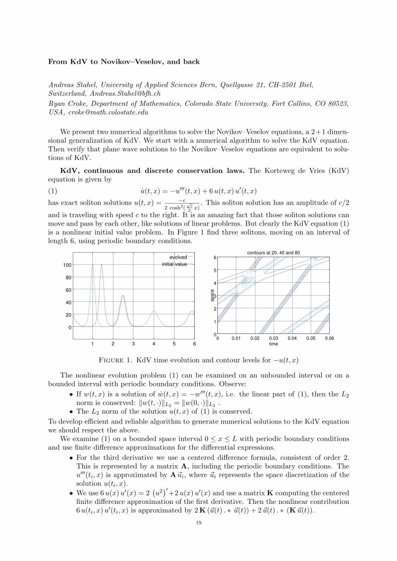
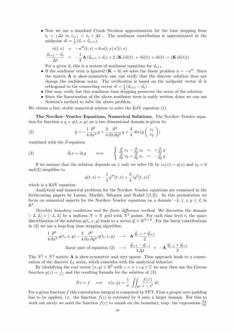
References
[1] Matti Lassas Jennifer L Mueller Samuli Siltanen and Andreas Stahel The Novikov-Veselov equation and the Inverse Scattering Method part i Analysis Physica D NonlinearPhenomena 2012
[2] Matti Lassas Jennifer L Mueller Samuli Siltanen and Andreas Stahel The Novikov-Veselov equation and the Inverse Scattering Method part ii Computation Nonlinearity 2012
Optical characterisation of nanostructures using a discretised forward model
Mirza Karamehmedovic Foundation Institute of Materials Science (IWT) Department ofProduction Engineering University of Bremen Badgasteiner Str 3 28359 BremenGermany mirzaiwtuni-bremende
Mads Peter Soslashrensen Department of Mathematics Technical University of DenmarkDK-2800 Kgs Lyngby Denmark MPSoerensenmatdtudk
Poul-Erik Hansen Danish Fundamental Metrology Technical University of DenmarkDK-2800 Kgs Lyngby Denmark pehdfmdtudk
Andrei V Lavrinenko DTU Fotonik Technical University of Denmark DK-2800 KgsLyngby Denmark
Optical diffraction microscopy (ODM) is a non-destructive and relatively inexpensive meansof characterisation of nanostructures It is an essential tool in the design production andquality control of functional nanomaterials In ODM the target is reconstructed from themeasured optical power in the reflected far field This inverse scattering problem is typicallyhighly ill-posed due to the incompleteness of the data and the low signal-to-noise ratio In arealistic setting the formulation of the forward scattering model is usually complicated by thepresence of supporting structures (eg a substrate or a grid supporting a nanoparticle) sincethe electromagnetic interaction between the nanostructure and the supporting structure mustbe taken into account Also the roughness and the contamination of the supporting structurecan increase the dimensionality and the ill-posedness of the inverse problem Finally the size ofthe measured nanostructure is typically comparable to the wavelength of the illuminating lightso the scattering needs to be described using the full Maxwellian electromagnetic model ratherthan (numerically inexpensive) asymptotic formulations
We here describe an efficient accurate and robust forward scattering model [12] based ondiscrete sources and tailor-made for the reconstruction of 2D nanoparticles on substrates fromODM data We adopt an analysis-based modelling paradigm and attempt to incorporate asmuch available a priori information as possible directly in the forward model We replacethe classical radiation integrals by finite linear combinations of stratified Greenrsquos functions forthe Helmholtz operator in the plane and thus achieve a sparse formulation and an implicitdescription of the particle-substrate interaction The forward model can be extended to includethe roughness and contamination of the substrate without sacrificing the speed of computation[3] We validate the model and show its feasibility in a decomposition-type inverse schemewith synthetic measurement data ([1] figure 1) as well as in the inversion of experimentalscatterometric data ([4] figure 2) Finally we use a related forward model in the inversion ofsynthetic measurement data to estimate aperiodic defects in a nanograting ([5] figure 3)
References
[1] M Karamehmedovic P-E Hansen and T Wriedt A fast inversion method for highlyconductive submicron wires on a substrate Journal of the European Optical Society ndash RapidPublications 6(11039) 2011
22
Figure 1 Cross-section reconstruction for a highly conductive nanowire on asmooth Si substrate using synthetic data The forward model uses discretesources Bottom the reconstructed near-field amplitude (left) and phase (right)
[2] M Karamehmedovic P-E Hansen and T Wriedt An efficient scattering model forPEC and penetrable nanowires on a dielectric substrate Journal of the European Optical Societyndash Rapid Publications 6(11021) 2011
[3] M Karamehmedovic P-E Hansen and T Wriedt An efficient rough-interface scat-tering model for embedded nanostructures Thin Solid Films DOI 101016jtsf2012110482012
[4] M Karamehmedovic P-E Hansen K Dirscherl E Karamehmedovic and T WriedtProfile estimation for Pt submicron wire on rough Si substrate from experimental data OpticsExpress 20(19) 21678ndash21686 2012
[5] M Karamehmedovic M P Soslashrensen P-E Hansen and A V Lavrinenko Applicationof the method of auxiliary sources to a defect-detection inverse problem of optical diffractionmicroscopy Journal of the European Optical Society ndash Rapid Publications 5(10021) 2010
23
Figure 2 Cross-section reconstruction for a Pt nanowire on a rough contam-inated Si substrate using experimental ODM data The forward model usesdiscrete sources Top SEM and AFM images of the nanowire Bottom theforward scattering model and the reconstructed near-field amplitude
Figure 3 Left a nanograting defect to be characterised by ODM with thediscrete sources forward model Right a FEM computation of the amplitude ofthe scattered near field for the defect-free scatterer
24
A SECOND DEGREE NEWTONrsquoS METHOD IN INVERSE SCATTERING
PROBLEM
RAINER KRESS AND KUO-MING LEE
The inverse problem of recovering the geometry and the physical properties of a scatterer from theknowledge of the far field pattern of the scattered field is of fundamental importance for example innon-destructive testing seismic research or medical imaging In this talk we consider as a model thetime-harmonic scattering problem from a sound-soft obstacle The aim of our inverse problem is torecover the unknown scatterer from the knowledge of the far field pattern
Based on integral equation the scattering problem can be formulated in the following operator form
(01) F (Γ) = uinfin
Indeed for the direct problem this equation gives the far field pattern uinfin from the knowledge of theboundary Γ of the obstacle with a given incident wave For the inverse problem one would like to findthe unknown boundary Γ from the (measured) far field data by solving this so-called far field equation(01) As opposed to the direct problem which is linear and well-posed in the sense of Hadamard theinverse problem is nonlinear and ill-posed Hence both linearization and regularization are needed at thesame time Because of its conceptual simplicity and accuracy of the reconstruction Newtonrsquos method is agood candidate for the linearization of the inverse problem The familiar Newtonrsquos method approximatesthe nonlinear operator via a linear one which is just the first derivative of the original one Here byreplacing the linear approximation of the nonlinear operator with a second degree approximation wewant to investigate whether the numerical performance can be improved Furthermore our second degreemethod can be carried out via two consecutive linear steps This is advantageous in the sense that thewhole inverse scheme remains in the setting of linear regularization theory
References
[1] R Kress and K-M Lee A second degree Newton method for an inverse obstacle scattering problem Journal ofComputational Physics 20 (2011) 761ndash769
Institut fur Numerische und Angewandte Mathematik University of Gottingen 37083 Gottingen Germany
E-mail address kressmathuni-goettingende
Department of Mathematics National Cheng Kung University701 Tainan Taiwan
E-mail address kmleemailnckuedutw
WORKSHOP bdquoINVERSE PROBLEMS AND NUMERICAL METHODS IN APPLICATIONSldquo
Title of presentation Determination of Heat Transfer Coefficients from cooling curves ndash an inverse problem of heat conduction Author
Thomas Luumlbben Affiliation
Stiftung Institut fuumlr Werkstofftechnik IWT Division Materials Science Department Heat treatment Badgasteiner Str 3 Germany luebbeniwt-bremende
Abstract One of the most important processes in heat treatment is the hardening process Aim of it is the increase of hardness (mechanical resistance against a mechanical penetration of a harder test body) and strength (maximum stress until cracking) To do this for steels the component has to be heated to a steel specific temperature During this process the steel will undergo a phase transformation The cubic body centered lattice will change to the cubic face centered one (called austenite) Furthermore carbides will be dissolved and the carbon will be distributed homogeneously by diffusion processes in the component This is possible because the austenite can assimilate much more carbon than the ferritic phases with cbc lattice In the second step the component has to be cooled with an overcritical steel depending cooling rate to avoid that the carbon atoms leave their position by diffusion and to achieve the phase martensite with a significant increase of hardness and strength This cooling process is called quenching and two research groups at IWT are working on this topic The group ldquoMultiphase Flow Heat- and Mass-Transferrdquo of Udo Fritsching (division ldquoProcess amp Chemical Engineering) is dealing with modeling and simulation of multiphase flowing systems by Computational Fluid Dynamics (CFD) The group of Thomas Luumlbben works on heat treatment simulation and needs the Heat Transfer Coefficient (HTC) as boundary condition to the solution of the heat conduction equation (material properties are temperature and phase dependent)
Q)grad(divt
cp +θsdotλ=partθpart
sdotsdotρ (1)
ρ [kgmsup3] density of the steel (temperature and phase dependent) cp [J(kgK)] specific heat capacity of the steel (temperature and phase dependent) λ [W(mK)] heat conductivity of the steel (temperature and phase dependent) Q [Wmsup3] intensity of internal heat sources (in general time dependent) θ [degC] temperature t [s] time For quenching media which exhibit only convective heat transfer as gases molten salts or water with a very high velocity (in the order of 10 ms) the HTC calculated by CFD can be used for heat treatment simulation CFD delivers the HTC for the complete surface of a component and if necessary even the corresponding time dependencies But in general a calibration of the model has to be done by a HTC
measurement Equation (1) can be simplified if no axial und circumferential heat flux occurs For a cylindrical body without phase transformations equation (2) results
θ (2) r [m] coordinate in radial direction By measuring the temperature near to the surface in the middle plane of the cylinder the inverse heat conduction problem for this simple case can be solved by optimization methods or by an inverse calculation by use of Dirichlet-condition For quenching media with a boiling temperature lower than the start temperature of the austenitized components (water and special oils) the heat transfer is much more complicated Two phases of the fluid have to be taken into account the liquid and the vapor of this liquid Instead of one mechanism two additional ones have to be considered film boiling and nucleate boiling A typical local temperature dependency of the HTC of a quenching oil is shown in the left figure
HTC as function of surface temperature (left) and
typical behavior of rewetting (right FP film boiling KP nucleate boiling Kon convection) After immersion of the component into the quenching media a prompt evaporation of the oil directly at the surface occur and vapor film is formed around the component This film acts as isolator and the resulting HTC is quite small After some time the vapor film breaks down at the lower edge of the cylinder and nucleate boiling starts (right figure) As a result of the direct contact between fluid and surface the HTC increases dramatically The front between film and nucleate boiling moves (rewetting) and after the local temperature drops below the boiling temperature convection starts In some cases a second front starts at the upper edge In consequence a complicated distribution of the HTC results with axial and in general circumferential heat fluxes Therefore the assumptions described above are not fulfilled and equation (2) cannot be used under these conditions But with special equipment circumferential heat fluxes can be avoided Than by use of
θ λ (3) z [m] coordinate in axial direction the problem has to be solved Again optimization methods can be used But investigations from literature show that the evaluation time for the method which provides acceptable results is comparable high (74 hours) For this reason a cooperation with the ldquoZentrum fuumlr Technomathematikrdquo (ZeTem) at the University of Bremen was started Within the frame of a modeling seminar two students started with the development of software tools for the estimation of the HTC as function of temperature and position In the lecture some results were presented and resulting problems discussed
A SIMULTANEOUS LINEARIZATION METHOD FOR INVERSE
SCATTERING PROBLEM FOR A DIELECTRIC
AHMET ALTUNDAG
Abstract The inverse problem under consideration is to reconstruct the shape of a homo-
geneous dielectric infinite cylinder from the far field pattern for scattering of a time-harmonic
E-polarized electromagnetic plane wave We propose an inverse algorithm that extends the ap-proach suggested by Kress and Rundell [13] and further investigated by Ivanyshyn and Kress
[5 6] for the case of the inverse problem for a perfectly conducting scatterer to the case of
penetrable scatter It is based on a system of nonlinear boundary integral equations associatedwith a single-layer potential approach to solve the forward scattering problem We present the
mathematical foundations of the method and exhibit its feasibility by numerical examples
1 Introduction
In inverse obstacle scattering problems for time-harmonic waves the scattering object is a ho-mogeneous obstacle and the inverse problem is to obtain an image of the scattering object iean image of the shape of the obstacle from a knowledge of the scattered wave at large distancesie from the far field pattern In the current paper we deal with dielectric scatterers and confineourselves to the case of infinitely long cylinders
Assume that the simply connected bounded domain D sub IR2 with C2 boundary partD representsthe cross section of a dielectric infinite cylinder having constant wave number kd with Re kd gt 0and Im kd ge 0 embedded in a homogeneous background with positive wave number k0 Denote byν the outward unit normal to partD Then given an incident plane wave ui(x) = eik0 xmiddotd with incidentdirection given by the unit vector d the direct scattering problem for Endashpolarized electromagneticwaves is modeled by the following transmission problem for the Helmholtz equation Find solutionsu isin H1
loc(IR2 D) and v isin H1(D) to the Helmholtz equations
(11) 4u+ k20u = 0 in IR2 D 4v + k2dv = 0 in D
satisfying the transmission conditions
(12) u = vpartu
partν=partv
partνon partD
in the trace sense such that u = ui + us with the scattered wave us fulfilling the Sommerfeldradiation condition
(13) limrrarrinfin
r12(partus
partrminus ik0us
)= 0 r = |x|
uniformly with respect to all directions The latter is equivalent to an asymptotic behavior of theform
(14) us(x) =eik0|x|radic|x|
uinfin
(x
|x|
)+O
(1
|x|
) |x| rarr infin
Key words and phrases inverse scattering Helmholtz equation transmission problem singlelayer approachnonlinear integral equations iterative methods
1
2A SIMULTANEOUS LINEARIZATION METHOD FOR INVERSE SCATTERING PROBLEM FOR A DIELECTRIC
uniformly in all directions with the far field pattern uinfin defined on the unit circle S1 in IR2
(see[4]) In the above u and v represent the electric field that is parallel to the cylinder axis (11)corresponds to the time-harmonic Maxwell equations and the transmission conditions (12) modelthe continuity of the tangential components of the electric and magnetic field across the interfacepartD
The inverse obstacle problem we are interested in is given the far field pattern uinfin for oneincident plane wave with incident direction d isin S1 to determine the boundary partD of the scatteringdielectric D More generally we also consider the reconstruction of partD from the far field patternsfor a small finite number of incident plane waves with different incident directions This inverseproblem is nonlinear and ill-posed since the solution of the scattering problem (11)ndash(13) is non-linear with respect to the boundary and since the mapping from the boundary into the far fieldpattern is extremely smoothing
At this point we note that uniqueness results for this inverse transmission problem are onlyavailable for the case of infinitely many incident waves (see [9]) A general uniqueness result basedon the far field pattern for one or finitely many incident waves is still lacking More recently auniqueness result for recovering a dielectric disk from the far field pattern for scattering of oneincident plane wave was established by Altundag and Kress [2]
In the spirit of the approach for scattering from a perfect conductor proposed by Kress andRundell [15] in electrostatics and further investigated by Ivanyshyn and Kress [7] in electromag-netics
For a stable solution of the inverse transmission problem we propose an algorithm that extendsthe approach suggested by Kress and Rundell [13] in electromagnetics and further investigatedby Kress and Ivanyshyn [5 6] for the case of the inverse problem for a perfectly conductingscatterer Representing the solution v and us to the forward scattering problem in terms of single-layer potentials in D and in IR2 D with densities ϕd and ϕ0 respectively the transmissioncondition (12) provides a system of two boundary integral equations on partD for the correspondingdensities that in the sequel we will denote as field equations For the inverse problem the requiredcoincidence of the far field of the single-layer potential representing us and the given far field uinfinprovides a further equation that we denote as data equation The system of the field and dataequations can be viewed as three equations for three unknowns ie the two densities and theboundary curve They are linear with respect to the densities and nonlinear with respect to theboundary curve
In the spirit of [5 6 13] given an approximation partDapprox for the boundary partD and approxi-mations ϕdapprox and ϕ0approx for the densities ϕd and ϕ0 we linearize both the field and the dataequations simultaneously with respect to the boundary curve and the two densities The linearequations are then solved to update both the boundary curve and the two densities Because of theill-posedness the solution of the update equations require stabilization for example by Tikhonovregularization This procedure is then iterated until some suitable stopping criterion is satisfied
The plan of the paper is as follows In Section 2 as ingredient of our inverse algorithm wedescribe the solution of the forward scattering problem via a single-layer approach followed by acorresponding numerical solution method in Section 3 The details of the inverse algorithm arepresented in Section 4 and in Section 5 we demonstrate the feasibility of the method by somenumerical examples
2 The direct problem
The forward scattering problem (11)ndash(13) has at most one solution (see [3 12] for the three-dimensional case) Existence can be proven via boundary integral equations by a combined single-and double-layer approach (see [3 12] for the three-dimensional case) Here we base the solution
A SIMULTANEOUS LINEARIZATION METHOD FOR INVERSE SCATTERING PROBLEM FOR A DIELECTRIC3
of the forward problem on a single-layer approach as investigated in [2] For this we denote by
Φk(x y) =i
4H
(1)0 (k|xminus y|) x 6= y
the fundamental solution to the the Helmholtz equation with wave number k in IR2 in terms of the
Hankel function H(1)0 of order zero and of the first kind Adopting the notation of [4] in a Sobolev
space setting for k = kd and k = k0 we introduce the single-layer potential operators
Sk Hminus12(partD)rarr H12(partD)
by
(25) (Skϕ)(x) = 2
int
partD
Φk(x y)ϕ(y) ds(y) x isin partD
and the normal derivative operators
K primek Hminus12(partD)rarr Hminus12(partD)
by
(26) (K primekϕ)(x) = 2
int
partD
partΦk(x y)
partν(x)ϕ(y) ds(y) x isin partD
For the Sobolev spaces and the mapping properties of these operators we refer to [11 17]Then from the jump relations it can be seen that the single-layer potentials
(27)
v(x) =
int
partD
Φkd(x y)ϕd(y) ds(y) x isin D
us(x) =
int
partD
Φk0(x y)ϕ0(y) ds(y) x isin IR2 D
solve the scattering problem (11)ndash(13) provided the densities ϕd and ϕ0 satisfy the system ofintegral equations
(28)
Skdϕd minus Sk0ϕ0 = 2ui|partD
ϕd +K primekdϕd + ϕ0 minusK primek0ϕ0 = 2partui
partν
∣∣∣∣partD
which in the squel we will call the field equations Provided k0 is not a Dirichlet eigenvalue of thenegative Laplacian for the domain D with the aid of the Riesz-Fredholm theory in [2] it has beenshown that the system (28) has a unique solution in Hminus12(partD)timesHminus12(partD) Thus throughoutthis paper we shall assume that k0 is not a Dirichlet eigenvalue of the negative Laplacian for thedomain D
After introducing the far field operator Sinfin Hminus12(partD)rarr L2(S1) by
(29) (Sinfinϕ)(x) = γ
int
partD
eminusik0 xmiddotyϕ(y) ds(y) x isin S1
from (27) and asymptotics of the Hankel function we observe that the far field pattern for thesolution to the scattering problem (11)ndash(13) is given by
(210) uinfin = Sinfinϕ0
in terms of the solution to (28)
4A SIMULTANEOUS LINEARIZATION METHOD FOR INVERSE SCATTERING PROBLEM FOR A DIELECTRIC
3 Numerical solution
For the numerical solution of (28) and the presentation of our inverse algorithm we assume thatthe boundary curve partD is given by a regular 2πndashperiodic parameterization
(31) partD = z(t) 0 le t le 2π
Then via ψ = ϕ z emphasizing the dependence of the operators on the boundary curve weintroduce the parameterized single-layer operator
Sk Hminus12[0 2π]times C2[0 2π]rarr H12[0 2π]
by
Sk(ψ z)(t) =i
2
int 2π
0
H(1)0 (k|z(t)minus z(τ)|) |zprime(τ)|ψ(τ) dτ
and the parameterized normal derivative operators
K primek Hminus12[0 2π]times C2[0 2π]rarr Hminus12[0 2π]
by
K primek(ψ z)(t) =ik
2
int 2π
0
[zprime(t)]perp middot [z(τ)minus z(t)]|zprime(t)| |z(t)minus z(τ)| H
(1)1 (k|z(t)minus z(τ)|) |zprime(τ)|ψ(τ) dτ
for t isin [0 2π] Here we made use of H(1)prime0 = minusH(1)
1 with the Hankel function H(1)1 of order zero
and of the first kind Furthermore we write aperp = (a2minusa1) for any vector a = (a1 a2) that is aperp
is obtained by rotating a clockwise by 90 degrees Then the parameterized form of (28) is givenby
(32)
Skd(ψd z)minus Sk0(ψ0 z) = 2ui z
ψd + K primekd(ψd z) + ψ0 minus K primek0(ψ0 z) =2
|zprime| [zprime]perp middot gradui z
The kernels
M(t τ) =i
2H
(1)0 (k|z(t)minus z(τ)|) |zprime(τ)|
and
L(t τ) =ik
2
[zprime(t)]perp middot [z(τ)minus z(t)]|zprime(t)| |z(t)minus z(τ)| H
(1)1 (k|z(t)minus z(τ)|) |zprime(τ)|
of the operators Sk and K primek can be written in the form
(33)
M(t τ) = M1(t τ) ln
(4 sin2 tminus τ
2
)+M2(t τ)
L(t τ) = L1(t τ) ln
(4 sin2 tminus τ
2
)+ L2(t τ)
A SIMULTANEOUS LINEARIZATION METHOD FOR INVERSE SCATTERING PROBLEM FOR A DIELECTRIC5
where
M1(t τ) = minus 1
2πJ0(k|z(t)minus z(τ)|)|zprime(τ)|
M2(t τ) = M(t τ)minusM1(t τ) ln
(4 sin2 tminus τ
2
)
L1(t τ) = minus k
2π
[zprime(t)]perp middot [z(τ)minus z(t)]|zprime(t)| |z(t)minus z(τ)| J1(k|z(t)minus z(τ)|) |zprime(τ)|
L2(t τ) = L(t τ)minus L1(t τ) ln
(4 sin2 tminus τ
2
)
The functions M1M2 L1 and L2 turn out to be smooth with diagonal terms
M2(t t) =
[i
2minus C
πminus 1
πln
(k
2|zprime(t)|
)]|zprime(t)|
in terms of Eulerrsquos constant C and
L2(t t) = minus 1
2π
[zprime(t)]perp middot zprimeprime(t)|zprime1(t)|2
For integral equations with kernels of the form (33) a combined collocation and quadrature meth-ods based on trigonometric interpolation as described in Section 35 of [4] or in [16] is at ourdisposal We refrain from repeating the details For a related error analysis we refer to [11] andnote that we have exponential convergence for smooth ie analytic boundary curves partD
For a numerical example we consider the scattering of a plane wave by a dielectric cylinder with anon-convex kite-shaped cross section with boundary partD described by the parametric representation
(34) z(t) = (cos t+ 065 cos 2tminus 065 15 sin t) 0 le t le 2π
From the asymptotics for the Hankel functions it can be deduced that the far field pattern ofthe single-layer potential us with density ϕ0 is given by
(35) uinfin(x) = γ
int
partD
eminusik0 xmiddotyϕ0(y) ds(y) x isin S1
where
γ =eiπ4radic
8πk0
The latter expression can be evaluated by the composite trapezoidal rule after solving the systemof integral equations (28) for ϕ0 ie after solving (32) for ψ0 Table 31 gives some approximatevalues for the far field pattern uinfin(d) and uinfin(minusd) in the forward direction d and the backwarddirection minusd The direction d of the incident wave is d = (1 0) and the wave numbers are k0 = 1and kd = 2 + 3i Note that the exponential convergence is clearly exhibited
6A SIMULTANEOUS LINEARIZATION METHOD FOR INVERSE SCATTERING PROBLEM FOR A DIELECTRIC
Table 31 Numerical results for direct scattering problem
n Reuinfin(d) Imuinfin(d) Reuinfin(minusd) Imuinfin(minusd)
8 -06017247940 -00053550779 -02460323014 0318495776816 -06018967551 -00056192337 -02461831740 0318605268632 -06019018135 -00056277492 -02461946976 0318604994964 -06019018076 -00056277397 -02461946846 03186049951
4 The inverse problem
We now proceed describing an iterative algorithm for approximately solving the inverse scatter-ing problem by extending the method proposed by Kress [13] and further investigated by Ivanyshynand Kress [5 6] for the case of the inverse problem for a perfectly conducting scatterer to the caseof a dielectric scatterer
After introducing the far field operator Sinfin Hminus12(partD)rarr L2(S1) by
(41) (Sinfinϕ)(x) = γ
int
partD
eminusik0 xmiddotyϕ(y) ds(y) x isin S1
from (27) and (35) we observe that the far field pattern for the solution to the scattering problem(11)ndash(13) is given by
(42) uinfin = Sinfinϕ0
in terms of the solution to (28)
41 The inverse problem for shape reconstruction We can state the following theorem astheoretical basis of our inverse algorithm For this we note that all our integral operators dependon the boundary curve partD
Theorem 41 For a given incident field ui and a given far field pattern uinfin assume that partD andthe densities ϕd and ϕ0 satisfy the system of three integral equations
(43)
Skdϕd minus Sk0ϕ0 = 2ui
ϕd +K primekdϕd + ϕ0 minusK primek0ϕ0 = 2partui
partν
Sinfinϕ0 = uinfin
Then partD solves the inverse problem
The ill-posedness of the inverse problem is reflected through the ill-posedness of the third integralequation the far field equation that we denote as data equation Note that (43) is linear withrespect to the densities and nonlinear with respect to the boundary partD This opens up a varietyof approaches to solve (43) by linearization and iteration In [2] we investigated an extensionof the approach suggested by Johansson and Sleeman [8] for a perfectly conducting scattererGiven a current approximation partDapprox for the unknown boundary partD we first solved the firsttwo equations or field equations of system (43) for the unknown densities ϕd and ϕ0 Thenkeeping ϕ0 fixed we linearized the third equation or data equation of system (43) with respectto the boundary partD to update the approximation Here following [5 6 13] we are going toproceed differently given an approximation partDapprox for the boundary partD and approximationsϕdapprox and ϕ0approx for the densities ϕd and ϕ0 we linearize both the field and the data equationssimultaneously with respect to the boundary curve and the two densities The linear equations are
A SIMULTANEOUS LINEARIZATION METHOD FOR INVERSE SCATTERING PROBLEM FOR A DIELECTRIC7
then solved to update both the boundary curve and the two densities Because of the ill-posednessthe solution of the update equations require stabilization for example by Tikhonov regularizationThis procedure is then iterated until some suitable stopping criterion is satisfied
To describe this in more detail we also require the parameterized version
Sinfin Hminus12[0 2π]times C2[0 2π]rarr L2(S1)
of the far field operator as given by
(44) Sinfin(ψ z)(x) = γ
int 2π
0
eminusik0 xmiddotz(τ)ψ(τ) dτ x isin S1
Then the parameterized form of (43) is given by
(45)
Skd(ψd z)minus Sk0(ψ0 z) = 2ui z
ψd + K primekd(ψd z) + ψ0 minus K primek0(ψ0 z) =2
|zprime| [zprime]perp middot gradui z
Sinfin(ψ0 z) = uinfin
For a fixed ψ the Frechet derivative of the operator Sk and K primek with respect to the boundary zin the direction h are given by (see [18])
Sprimek(ψ zh)(t) =minusik
2
int 2π
0
(z(t)minus z(τ)) middot (h(t)minus h(τ))
|z(t)minus z(τ)| |zprime(τ)|H(1)1 (k|z(t)minus z(τ)|)ψ(τ)dτ
+i
2
int 2π
0
zprime(τ) middot hprime(τ)
|zprime(τ)| H(1)0 (k|z(t)minus z(τ)|)ψ(τ)dτ(46)
and(47)
(K primek)prime(ψ zh)(t) =
minus ik
2|zprime(t)|int 2π
0
[zprime(t)]perpmiddot(h(t)minush(τ))+[hprime(t)]perpmiddot(z(t)minusz(τ))
|z(t)minusz(τ)| |zprime(τ)|H(1)1 (k|z(t)minusz(τ)|)ψ(τ)dτ
+ik
|zprime(t)|
int 2π
0
[zprime(t)]perpmiddot(z(t)minusz(τ))(h(t)minush(τ))middot(z(t)minusz(τ))
|z(t)minusz(τ)|3 |zprime(τ)|H(1)1 (k|z(t)minusz(τ)|)ψ(τ)dτ
minus ik2
2|zprime(t)|
int 2π
0
[zprime(t)]perpmiddot(z(t)minusz(τ))(h(t)minush(τ))middot(z(t)minusz(τ))
|z(t)minusz(τ)|2 |zprime(τ)|H(1)0 (k|z(t)minusz(τ)|)ψ(τ)dτ
+ik
2
hprime(t) middotzprime(t)|zprime(t)|2
int 2π
0
[zprime(t)]perp middot(z(t)minusz(τ))
|z(t)minus z(τ)| |zprime(τ)|H(1)1 (k|z(t)minusz(τ)|)ψ(τ)dτ
minus ik
2|zprime(t)|
int 2π
0
[zprime(t)]perp middot(z(t)minusz(τ))hprime(τ)middotzprime(τ)
|z(t)minusz(τ)||zprime(τ)| H(1)1 (k|z(t)minusz(τ)|)ψ(τ)dτ
8A SIMULTANEOUS LINEARIZATION METHOD FOR INVERSE SCATTERING PROBLEM FOR A DIELECTRIC
Then the linearization (45) with respect to all variables z ϕd and ϕ0 in the direction h ηd andη0 respectively reads
(48)
Skd(ψd z) + Skd(ηd z) + Sprimekd(ψd zh)minus Sk0(ψ0 z)minus Sk0(η0 z)
minusSprimek0(ψ0 zh) = 2ui z + 2gradui z middot h
ψd + ηd + ψ0 + η0 + K primekd(ψd z) + K primekd(ηd z) + (K primed)prime(ψd zh)
minusK primek0(ψ0 z)minus K primek0(η0 z)minus (K primek0)prime(ψ0 zh) =2
|zprime| [zprime]perp middot gradui z + 2ξ(z) middot h
Sinfin(ψ0 z) + Sinfin(η0 z) + Sprimeinfin(ψ0 zh) = uinfin
Here the term ξ(z) middot h is the form ( see [19 20])
(49) ξ(z) middot h = minuspartui
partτ
ν middot hprime|zprime| + (
part2ui
partνpartτminusHpartui
partτ)τ middot h+
part2ui
partν2ν middot h
and τ and H stand for the tangential vector and the mean curvature respectively They are givenby
τ =zprime
|zprime| and H = minuszprimeprime middot ν|zprime|2
and the matrix form of (48) can be written as
(410)
Sprimekd(ψd z middot)minus Sprimek0(ψ0 z middot)minus 2gradui z Skd(middot z) minusSk0(middot z)
(K primekd)prime(ψd z middot)minus (K primek0)prime(ψ0 z middot)minus 2ξ(z) I + K primekd(middot z) I minus K primek0(middot z)
Sprimeinfin(ψ0 z middot) 0 Sinfin(middot z)
h
ηd
η0
=
2ui z minus Skd(ψd z) + Sk0(ψ0 z)
2
|zprime| [zprime]perp middot gradui z minus ψd minus K primekd(ψd z)minus ψ0 + K primek0(ψ0 z)
uinfin minus Sinfin(ψ0 z)
Now we can describe the method in a short form as follows
Each iteration step of the proposed inverse algorithm consists of one part
bull Given an approximation z for the boundary and densities ψd ψ0 we solve the linearizedsistem of integral equations (410) for h ηd and η0 to obtain updates z + h ψd + ηd andψ0 +η0 We continue this procedure until some stopping criteria is achieved The stoppingcriterion for the iterative scheme is given by the relative error
(411) uinfinN minus uinfin uinfin
le ε
where uinfinN is the computed far field pattern after N iteration steps
A SIMULTANEOUS LINEARIZATION METHOD FOR INVERSE SCATTERING PROBLEM FOR A DIELECTRIC9
Here we note that only in the first iteration step it is convenient to start from an approximationz for the boundary and solve the first two equations in (45) for the densities
Because of the ill-posedness the solution of (410) requires stabilization for instance by Tikhonovregularization We choose for the boundary Hp penalty term and the regularization parameterλ = (08)j decreasing with the iteration step j and for the densities L2 penalty term and theregularization parameter α = 10minus6
In principle the parameterization of the update is not unique To cope with this ambiguityone possibility that we will pursue in our numerical examples of the subsequent section is to allowonly parameterizations of the form
(412) z(t) = r(t)
(cos tsin t
) 0 le t le 2π
with a non-negative function r representing the radial distance of partD from the origin Consequentlythe perturbations are of the form
(413) h(t) = q(t)
(cos tsin t
) 0 le t le 2π
with a real function q In the approximations we assume r and its update q to have the form of atrigonometric polynomial of degree J in particular
(414) q(t) =
Jsum
j=0
aj cos jt+
Jsum
j=1
bj sin jt
Then the update equation (410) is solved in the least squares sense penalized via Tikhonov reg-ularization for the unknown coefficients a0 aJ and b1 bJ of the trigonometric polynomialrepresenting the update q As experienced in the application of the above approach for relatedproblems it is advantageous to use an Hp Sobolev penalty term rather than an L2 penalty in the
Tikhonov regularization ie to interpret Sprimek and (K primek)prime as ill-posed linear operators
(415) Sprimek Hp[0 2π]rarr L2[0 2π] (K primek)prime Hp[0 2π]rarr L2[0 2π]
for some small p isin INAs a theoretical basis for the application of Tikhonov regularization from [4] we cite that after
the restriction to star-like boundaries the operator Sprimek and (K primek)prime are injective provided k2 is nota Neumann eigenvalue for the negative Laplacian in D
The above algorithm has an extension for the case of more than one incident wave Assumethat ui1 u
iM are M incident waves with different incident directions and uinfin1 uinfinM the
corresponding far field patterns for scattering from partD Then the inverse problem to determinethe unknown boundary partD from these given far field patterns and incident fields is equivalent tosolve the following equation for the boundary z and densities ψd1 ψdM and ψ01 ψ0M
(416)
Skd(ψdm z)minus Sk0(ψ0m z) = 2uim z
ψdm + ψ0m + K primekd(ψdm z)minus K primek0(ψ0m z) =2
|zprime| [zprime]perp middot graduim z
Sinfin(ψ0m z) = uinfinm
10A SIMULTANEOUS LINEARIZATION METHOD FOR INVERSE SCATTERING PROBLEM FOR A DIELECTRIC
we simultaneously linearize the system (416) with respect to all 2M + 1 variables For fixed zψ0m and ψdm m = 1 M the linearized system of integral equations obtains the form(417)
Sprimekd(ψdmzh)minusSprimek0m(ψ0mzh)minus2graduimz middoth+Skd(ηdmz)minusSk0(η0mz)
=2uimzminusSkd(ψdm z)+Sk0(ψ0m z)
(K primekd)prime(ψdm zh)minus(K primek0)prime(ψ0mzh)minus2ξm(z)middoth+ ηdm +K primekd(ηdmz)+ η0m minusK primek0(η0mz)
=2
|zprime| [zprime]perp middotgraduimzminusψdmminusK primekd(ψdmz)minusψ0m+K primek0(ψ0mz)
Sprimeinfin(ψ0m zh) + Sinfin(η0m z) = uinfinm minus Sinfin(ψ0m z)
Each iteration step of the proposed inverse algorithm also consists of one part
bull Given an approximation z for the boundary and densities ψdm ψ0m we solve the linearized(417) for h ηdm and η0m to obtain updates z + h ψdm + ηdm and ψ0m + η0m form = 1 M
Here we again note that only in the first iteration step it is convenient to start from an initialguess z for the boundary and solve the first 2M equations in (416) for the densities
We continue this procedure until some suitable criteria is achieved The stopping criterion forthe iterative scheme is given by the relative error
(418) uinfinmN minus uinfinm
uinfinm le ε
for m = 1 M where uinfinmN are the computed far field patterns after N iteration stepsFor the ill-posedness we choose the same penalty terms and regularization parameters for the
case of one incident fieldFor the numerical implementation we need to discretize the boundary operator Sprimek in (46) The
kernels of the operator Sprimek can be written in the form
A(t τ) = minus ik2
(z(t)minus z(τ)) middot (h(t)minus h(τ))
|z(t)minus z(τ)| |zprime(τ)|H(1)1 (k|z(t)minus z(τ)|)
B(t τ) =i
2
zprime(τ) middot hprime(τ)
|zprime(τ)| H(1)0 (k|z(t)minus z(τ)|)
The kernels A and B can be expressed of the form
A(t τ) = A1(t τ) ln(4 sin2 tminus τ2
) +A2(t τ)
B(t τ) = B1(t τ) ln(4 sin2 tminus τ2
) +B2(t τ)
A SIMULTANEOUS LINEARIZATION METHOD FOR INVERSE SCATTERING PROBLEM FOR A DIELECTRIC11
where
A1(t τ) =k
2π
(z(t)minus z(τ)) middot (h(t)minus h(τ))
|z(t)minus z(τ)| |zprime(τ)| J1(k|z(t)minus z(τ)|)
A2(t τ) = A(t τ)minusA1(t τ) ln(4 sin2 tminus τ2
)
B1(t τ) = minus 1
2π
zprime(τ) middot hprime(τ)
|zprime(τ)| J0(k|z(t)minus z(τ)|)
B2(t τ) = B(t τ)minusB1(t τ) ln(4 sin2 tminus τ2
)
in terms of Bessel functions J0 and J1 The functions A1 A2B1 and B2 turn out to be smoothwith diagonal terms Their diagonal terms are in the form
A1(t t) = 0 amp A2(t t) = minus 1
π
zprime(t) middot hprime(t)|zprime(t)|
B1(t t) = minus 1
2π
zprime(t) middot hprime(t)|zprime(t)| amp B2(t t) =
i
2minus 1
πln
(k
2|zprime(t)|
)minus C
π
zprime(t) middot hprime(t)
in terms of Eulerrsquos constant C we also need to discretize the boundary operator K primek in (47) The
kernels of the operator (K primek)prime can be written in the form
C(t τ h k) =minusik([zprime(t)]perp middot (h(t)minus h(τ))+[hprime(t)]perp middot (z(t)minus z(τ)))
2|zprime(t)||z(t)minus z(τ)| |zprime(τ)|H(1)1 (k|z(t)minus z(τ)|)
D(t τ h k) =ik[zprime(t)]perp middot (z(t)minus z(τ))(h(t)minus h(τ))middot (z(t)minus z(τ))
|zprime(t)||z(t)minus z(τ)|3 |zprime(τ)|H(1)1 (k|z(t)minus z(τ)|)
E(t τ h k) =minusik2[zprime(t)]perpmiddot (z(t)minusz(τ))(h(t)minush(τ)) middot (z(t)minus z(τ))
2|zprime(t)||z(t)minus z(τ)|2 |zprime(τ)|H(1)0 (k|z(t)minusz(τ)|)
F (t τ h k) =ik
2
hprime(t) middot zprime(t)|zprime(t)|2
[zprime(t)]perp middot (z(t)minus z(τ))
|z(t)minus z(τ)| |zprime(τ)|H(1)1 (k|z(t)minus z(τ)|)
G(t τ h k) = minus ik
2|zprime(t)|[zprime(t)]perp middot (z(t)minus z(τ))hprime(τ) middot zprime(τ)
|z(t)minus z(τ)||zprime(τ)| H(1)1 (k|z(t)minus z(τ)|)
These kernels also can be expressed as following
C(t τ h k) = C1(t τ h k) ln(4 sin2 tminus τ2
) + C2(t τ h k)
D(t τ h k) = D1(t τ h k) ln(4 sin2 tminus τ2
) +D2(t τ h k)
E(t τ h k) = E1(t τ h k) ln(4 sin2 tminus τ2
) + E2(t τ h k)
F (t τ h k) = F1(t τ h k) ln(4 sin2 tminus τ2
) + F2(t τ h k)
G(t τ h k) = G1(t τ h k) ln(4 sin2 tminus τ2
) +G2(t τ h k)(419)
12A SIMULTANEOUS LINEARIZATION METHOD FOR INVERSE SCATTERING PROBLEM FOR A DIELECTRIC
where
C1(t τ h k) =k([zprime(t)]perp middot(h(t)minush(τ))+[hprime(t)]perp middot(z(t)minusz(τ)))
2π|zprime(t)||z(t)minus z(τ)| |zprime(τ)|J1(k|z(t)minusz(τ)|)
C2(t τ h k) = C(t τ h k)minus C1(t τ h k) ln(4 sin2 tminus τ2
)
D1(t τ h k) =minusk[zprime(t)]perp middot(z(t)minusz(τ))(h(t)minush(τ))middot(z(t)minusz(τ))
π|zprime(t)||z(t)minus z(τ)|3 |zprime(τ)|J1(k|z(t)minusz(τ)|)
D2(t τ h k) = D(t τ h k)minusD1(t τ h k) ln(4 sin2 tminus τ2
)
E1(t τ h k) =k2[zprime(t)]perp middot(z(t)minusz(τ))(h(t)minush(τ))middot(z(t)minus z(τ))
2π|zprime(t)||z(t)minus z(τ)|2 |zprime(τ)|J0(k|z(t)minusz(τ)|)
E2(t τ h k) = E(t τ h k)minus E1(t τ h k) ln(4 sin2 tminus τ2
)
F1(t τ h k) = minus k
2π
hprime(t) middot zprime(t)|zprime(t)|2
[zprime(t)]perp middot (z(t)minus z(τ))
|z(t)minus z(τ)| |zprime(τ)|J1(k|z(t)minus z(τ)|)
F2(t τ h k) = F (t τ h k)minus F1(t τ h k) ln(4 sin2 tminus τ2
)
G1(t τ h k) =k
2π
1
|zprime(t)|[zprime(t)]perp middot (z(t)minus z(τ))hprime(τ) middot zprime(τ)
|z(t)minus z(τ)||zprime(τ)| J1(k|z(t)minus z(τ)|)
G2(t τ h k) = G(t τ h k)minusG1(t τ h k) ln(4 sin2 tminus τ2
)
The functions C1 C2D1 D2 E1 E2F1 F2 G1 and G2 turn out to be smooth with diagonalterms Their diagonal terms are in the form
C1(t t) = 0 amp C2(t th) =1
2π
[zprime(t)]perp middot hprimeprime(t) + [hprime(t)]perp middot zprimeprime(t)|zprime(t)|2
D1(t t) = 0 amp D2(t th) = minus 1
π
[zprime(t)]perp middot zprimeprime(t) zprime(t) middot hprime(t)|zprime(t)|4
E1(t t) = 0 amp E2(t t) = 0
F1(t t) = 0 amp F2(t th) = minus 1
2π
[zprime(t)]perp middot zprimeprime(t) zprime(t) middot hprime(t)|zprime(t)|3
G1(t t) = 0 amp G2(t th) =1
2π
[zprime(t)]perp middot zprimeprime(t) zprime(t) middot hprime(t)|zprime(t)|4
5 Numerical examples
To avoid an inverse crime in our numerical examples the synthetic far field data were ob-tained by a numerical solution of the boundary integral equations based on a combined single-and double-layer approach (see [3 12]) using the numerical schemes as described in [4 10 11]For perturbed data we added normally distributed noise to the real and imaginary part of the farfield and measured the noise level in the L2 norm In each iteration step of the inverse algorithmfor the discretization of the linearized field equations we used the numerical method for the loga-rithmic kernels as described in [2] using 64 quadrature points The linearized data equation wasdiscretized by the composite trapezoidal rule again using 64 quadrature points For the Tikhonovregularization of the boundary parametrization we used an H2 penalty term
A SIMULTANEOUS LINEARIZATION METHOD FOR INVERSE SCATTERING PROBLEM FOR A DIELECTRIC13
Table 52 Parametric representation of boundary curves
Counter type Parametric representation
Apple-shaped z(t) = 05+04 cos t+01 sin 2t1+07 cos t
(cos t sin t) t isin [0 2π]
Dropped-shaped z(t) = (minus05 + 075 sin t2minus075 sin t) t isin [0 2π]
Kite-shaped z(t) = (cos t+ 13 cos2 tminus 13 15 sin t) t isin [0 2π]
Peanut-shaped z(t) = radiccos2 t+ 025 sin t (cos t sin t) t isin [0 2π]
Rounded triangle z(t) = (2 + 03 cos 3t)(cos t sin t) t isin [0 2π]
51 Numerical examples of shape reconstruction In all our five examples we used M = 8as a number of incident waves with the directions d = (cos(2πmM) sin(2πmM)) m = 1 Mand J = 5 as degree for the approximating trigonometric polynomials in (414) and N as thenumber of recursion and the wave numbers k0 = 1 and kd = 10 + 10i The initial guess isgiven by the green curve the exact boundary curves are given by the dashed (blue) lines and thereconstructions by the full (red) lines The iteration numbers and the regularization parametersα and λ for the densities and the boundary respectively were chosen by trial and error and theirvalues are indicated in the following description of the individual examples
In order to obtain noisy data random errors are added point-wise to uinfin
(51) uinfin = uinfin + δξ||uinfin|||ξ|
with the random variable ξ isin C and Re ξ Im ξ isin (0 1)In the first example Fig 1 shows reconstructions after N = 12 iterations with the regularization
parameters α = 10minus7 and λ = 08j decreasing with the iteration steps j For the stopping criteria(418) ε = 10minus3 is chosen
In the second example Fig 2 shows reconstructions after N = 12 iterations with the regular-ization parameter chosen as in the first example For the stopping criteria (418) ε = 10minus3 ischosen
In the third example the reconstructions in Fig 3 were obtained after N = 15 iterations with theregularization parameter chosen as in the first example For the stopping criteria (418) ε = 10minus2
is chosenIn the fourth example the reconstructions in Fig 4 were obtained after N = 12 iterations with
the regularization parameters chosen as α = 10minus6 and λ = 07j For the stopping criteria (418)ε = 10minus3 is chosen In the final example Fig 5 shows reconstructions after N = 14 iterations withthe regularization parameters chosen as α = 10minus7 and λ = 08j For the stopping criteria (418)ε = 10minus3 is chosen
14A SIMULTANEOUS LINEARIZATION METHOD FOR INVERSE SCATTERING PROBLEM FOR A DIELECTRIC
minus1 minus05 0 05 1minus1
minus08
minus06
minus04
minus02
0
02
04
06
08
1
reconstructedexactintminusguess
minus1 minus05 0 05 1minus1
minus08
minus06
minus04
minus02
0
02
04
06
08
1
reconstructedexactintminusguess
minus1 minus05 0 05 1minus1
minus08
minus06
minus04
minus02
0
02
04
06
08
1
reconstructedexactintminusguess
Figure 1 Reconstruction of the apple-shaped contour 52 for exact data (left)3 noise (middle) and 5 noise (right)
minus1 minus08 minus06 minus04 minus02 0 02 04 06 08
minus06
minus04
minus02
0
02
04
06
reconstructedexactintminusguess
minus1 minus08 minus06 minus04 minus02 0 02 04 06 08
minus06
minus04
minus02
0
02
04
06
reconstructedexactintminusguess
minus1 minus08 minus06 minus04 minus02 0 02 04 06 08
minus06
minus04
minus02
0
02
04
06
reconstructedexactintminusguess
Figure 2 Reconstruction of dropped-shaped contour 52 for exact data (left)3 noise (middle) and 5 noise (right)
minus2 minus15 minus1 minus05 0 05 1 15 2
minus15
minus1
minus05
0
05
1
15
reconstructedexactintminusguess
minus2 minus15 minus1 minus05 0 05 1 15 2
minus15
minus1
minus05
0
05
1
15
reconstructedexactintminusguess
minus2 minus15 minus1 minus05 0 05 1 15 2
minus15
minus1
minus05
0
05
1
15
reconstructedexactintminusguess
Figure 3 Reconstruction of kite-shaped contour 52 for exact data (left) 3noise (middle) and 5 noise (right)
Our examples clearly indicate the feasibility of the proposed algorithm From our further numer-ical experiments it is observed that using more than one incident wave improved on the accuracyof the reconstruction and the stability Furthermore an appropriate initial guess was importantto ensure numerical convergence of the iterations Our examples also indicate that the proposedalgorithm with the numerical reconstructions are superior to those obtained via by Johonsson andSleeman [8] in [2] This behaviour is confirmed by a number of further numerical examples in [1]Furthermore from the numerical example we also observe that the proposed algorithm is moretolerable to noise level then the method of Johanson and Sleeman [8] in [2]
A SIMULTANEOUS LINEARIZATION METHOD FOR INVERSE SCATTERING PROBLEM FOR A DIELECTRIC15
minus25 minus2 minus15 minus1 minus05 0 05 1 15 2 25minus2
minus15
minus1
minus05
0
05
1
15
2
reconstructedexactintminusguess
minus25 minus2 minus15 minus1 minus05 0 05 1 15 2 25minus2
minus15
minus1
minus05
0
05
1
15
2
reconstructedexactintminusguess
minus25 minus2 minus15 minus1 minus05 0 05 1 15 2 25minus2
minus15
minus1
minus05
0
05
1
15
2
reconstructedexactintminusguess
Figure 4 Reconstruction of peanut-shaped contour 52 for exact data (left) 3noise (middle) and 5 noise (right)
minus2 minus15 minus1 minus05 0 05 1 15 2 25
minus2
minus15
minus1
minus05
0
05
1
15
2
reconstructedexactintminusguess
minus2 minus15 minus1 minus05 0 05 1 15 2 25
minus2
minus15
minus1
minus05
0
05
1
15
2
reconstructedexactintminusguess
minus2 minus15 minus1 minus05 0 05 1 15 2 25
minus2
minus15
minus1
minus05
0
05
1
15
2
reconstructedexactintminusguess
Figure 5 Reconstruction of rounded-triangle-shaped contour 52 for exact data(left) 3 noise (middle) and 5 noise (right)
Further research will be directed towards applying the algorithm to real data to extend thenumerics to the three dimensional case as investigated for a impenetrable scatterer in [7]
Acknowledgments
The author thanks his supervisor Professor Rainer Kress for the discussion on the topic of this paperThis research was supported by the German Research Foundation DFG through the GraduiertenkollegIdentification in Mathematical Models
References
[1] Altundag A On a two-dimensional inverse scattering problem for a dielectric Dissertation Gottingen
February 2012[2] Altundag A and Kress R On a two dimensional inverse scattering problem for a dielectric Applicable
Analysis 91 pp 757ndash771 (2012)
[3] Colton D and Kress R Integral Equation Methods in Scattering Theory Wiley-Interscience PublicationsNew York 1983
[4] Colton D and Kress R Inverse Acoustic and Electromagnetic Scattering Theory 2nd ed Springer Berlin
1998[5] Ivanyshyn O and Kress R Nonlinear integral equations in inverse obstacle scattering In Mathematical
Methods in Scattering Theory and Biomedical Engineering (Fotiatis Massalas eds) World Scientific Singa-
pore pp 39-50 (2006)[6] IvanyshynO and KressR Nonlinear Integral Equations for solving inverse boundary value problems for
inclusions and cracks J Integral Equations Appl18 1(2006)13-38
[7] Ivanyshyn O Kress R and Serranho R Huygensrsquo principle and iterative methods in inverse obstaclescattering Advances in Computational Mathematics 33 pp 413ndash429 (2010)
16A SIMULTANEOUS LINEARIZATION METHOD FOR INVERSE SCATTERING PROBLEM FOR A DIELECTRIC
[8] Johansson T and Sleeman B Reconstruction of an acoustically sound-soft obstacle from one incident field
and the far-field pattern IMA Jour Appl Math 72 pp 96ndash112 (2007)
[9] Kirsch A and Kress R Uniqueness in inverse obstacle scattering Inverse Problems 9 pp 285ndash299 (1993)[10] Kress R On the numerical solution of a hypersingular integral equation in scattering theory J Comp Appl
Math 61 pp 345ndash360 (1995)
[11] Kress R Integral Equations 2nd ed Springer Verlag Berlin 1998[12] Kress R and Roach GF Transmission problems for the Helmholtz equation J Math Phys 19pp 1433ndash
1437 (1978)
[13] Kress R and Rundell W Nonlinear integral equations and the iterative solution for an inverse boundaryvalue problem Inverse Problems 21 pp 1207ndash1223 (2005)
[14] Kress R and Sloan IH On the numerical solution of a logarithmic integral equation of the first kind for the
Helmholtz equation Numerische Mathematik 66 pp 199ndash214 (1993)[15] McLean W Strongly Elliptic Systems and Boundary Integral Equations Cambridge University Press 2000
[16] Potthast R Frechet differentiability of boundary integral operators in inverse acoustic scattering InverseProblems 10 pp 431ndash447 (1994)
[17] Serranho P A hybrid method for inverse scattering for shape and impedance Inverse Problems 22 pp
663ndash680 (2006)[18] Serranho P A hybrid method for inverse obstacle scattering problems PhD thesis University of Gottingen
(2007)
Institut fur Numerische Angewandte Mathematik Universitat Gottingen 37083 Gottingen Ger-
manyE-mail address aaltundagmathuni-goettingende
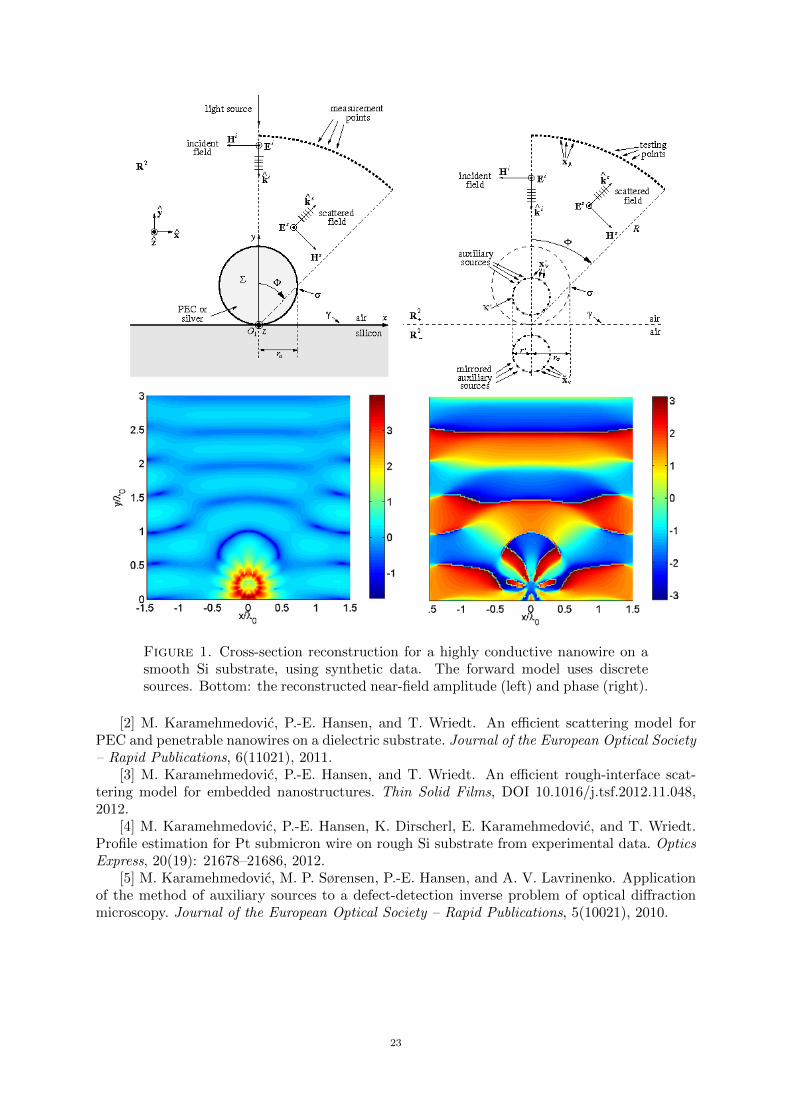
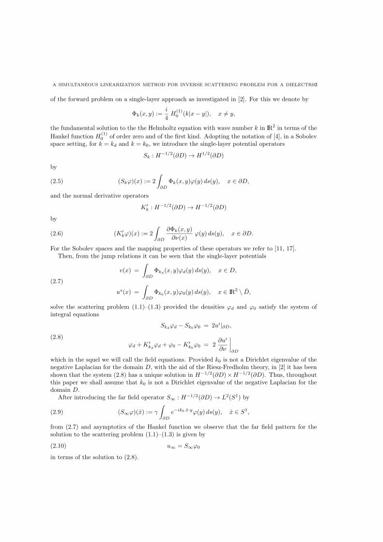
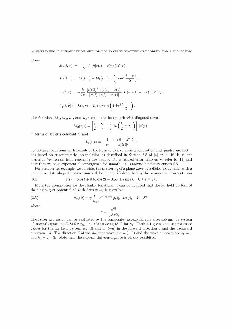
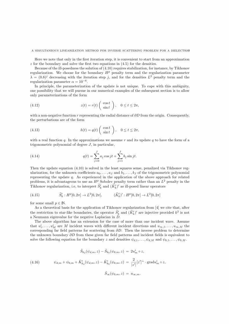
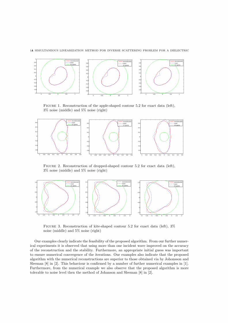