Embed Size (px)
Citation preview

Introduction to the course“Inverse problems: mathematical analysis and
numerical algorithms”
Laurent Bourgeois and Houssem Haddar
ENSTA / INRIA Saclay Ile de France / CMAP, Ecole Polytechnique
January 2013

Objective and program
This course addresses several theoretical and numerical questions related to theresolution of inverse problems arising in various fields: tomography, nondestructive testing, imaging,...
I Inverse problems: prototypes and examples (H.H. - 1)
I Regularization of linear ill-posed problems (H.H. - 2)
I Regularization of linear ill-posed problems (cont.) : the case of ill-posedCauchy problems (L.B. - 3, 4)
I Uniqueness and stability issues (L.B. - 5, 6)
I Algorithms for solving ill-posed Cauchy problems (L.B. - 7)
I Application to parameter identification (L.B. - 8)
I Non linear inverse problems and optimization methods (H.H. - 9)
I Inverse shape problems, the case of impedance tomography (H.H. - 10)
I Factorization method applied to impedance tomography (H.H. - 11, 12)

How can we define inverse problems?
First (naive) definition: The inverse map of a direct problem!
Example:
u 7→ u′
can be seen as the inverse problem associated with a direct problem
u 7→∫
u
Why not the reverse definition?
By convention, the direct problem is well posed (in the sense of Hadamard):Existence and Uniqueness of solutions + Stability (continuity) with respect todata.
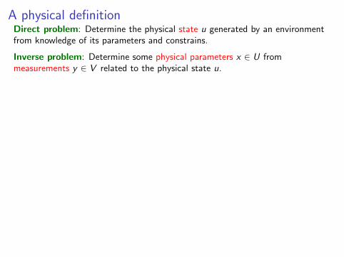
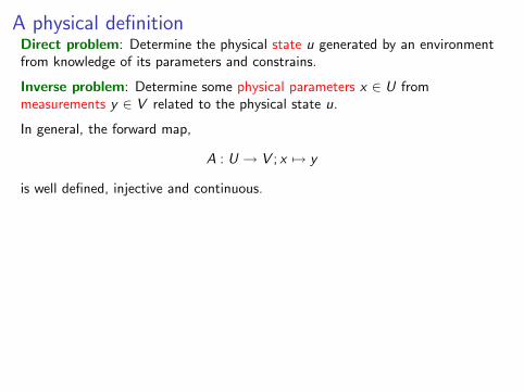
A physical definitionDirect problem: Determine the physical state u generated by an environmentfrom knowledge of its parameters and constrains.
Inverse problem: Determine some physical parameters x ∈ U frommeasurements y ∈ V related to the physical state u.
In general, the forward map,
A : U → V ; x 7→ y
is well defined, injective and continuous.
Typical problem for inverse problems: Measurements space is in general onlyL2 functions (due to lack of control of measurement errors). But state regularityis higher than L2.
⇒ In general, the closure of the range of A is compactly embedded in L2.
TheoremLet U and V be infinite dimensional vectorial spaces and A : U → V be aninjective and compact operator. Then A−1 : Range A ⊂ V → U cannot becontinuous.
⇒ the inverse problem y 7→ x is unstable.

Some academic examples
I Derivation is “unstable”
A : L2(0, 1)→ L2(0, 1), u 7→ x 7→∫ x
0
u(t)dt
I Inverse source problem
A : L2(Ω)→ L2(Ω), f 7→ u
where u ∈ H10 (Ω) is the unique solution of
−∆u = f in Ω.
I Initial data for diffusion problems (heat equation)
A : L2(0, π)→ L2(0, π), u0 7→ u(·,T )
where t 7→ u(·, t) ∈ H10 (0, π) is the unique continuous solution of
∂u∂t −∆u = 0 in (0, π)× (0,+∞),u(x , 0) = u0 in(0, π)

Prototype of linear ill posed problemsLet Ω1 ⊂ Rn1 , Ω2 ⊂ Rn2 be two open (measurable) sets.
TheoremLet K ∈ L2(Ω1 × Ω2) and define A : L2(Ω1)→ L2(Ω2) by
Af (x2) =
∫Ω1
K (x1, x2)f (x1) dx1, for a.e.x2 ∈ Ω2
Then A is continuous with ‖A‖ ≤ ‖K‖L2(Ω1×Ω2) and is also compact.
Definition: We say that A is an integral operator with kernal K .
Corollary: The inverse problem associated with Af = u is unstable for linearintegral operator with L2 kernels.
Remark 1: All previous examples fall in this class.
Remark 2: Convolution operators
Af (x2) =
∫Ω1
k(x2 − x1)f (x1) dx1, for a.e.x2 ∈ Ω2
with compactly supported and bounded kernels k are also typical examples ofthese operators (⇒ models for blurred images).

Two prototype of nonlinear inverse problems
I Parameter identification of PDE from partial measurements of the solutions
I Shape identification of boundaries or parameter discontinuities location

First model problem: corrosion/deposit detection
Ω
Accessible boundary Γ0
Unaccessible boundary Γ1
I Ω is a conducting material. E = ∇u,
∆u = 0 in Ω
I We apply current g = ∇u · n on Γ0
I Γ1 is buried part that may be corroded: corrosion model
∂u/∂n + λu = 0 on Γ1 = ∂Ω \ Γ0
Direct problem: λ ∈ L∞(Γ1) 7→ u|Γ0∈ L2(Γ0)
Inverse (Cauchy) problem: u|Γ0∈ L2(Γ0) 7→ λ = −u/(∂u/∂n) ∈ L∞(Γ1)

Example of applications: Non destructive testing of nuclearfuel rods

Second model problem: Electrical Impedance Tomographyσ = σ0
Inclusions with σ 6= σ0
Ω
I Inclusions (cancerous cells, blood containing regions, etc) have differentconductivity than the conductivity of the other components.
divσ∇u = 0 in Ω
I We apply different currents g = ∇u · n on ∂Ω
Direct problems: σ ∈ L∞(Ω) 7→ f = u|∂Ω ∈ L2(∂Ω)
We formally denote Λ(σ) : g 7→ f
Inverse problem 1 (parameter identification): Determine σ from the knowledgeof Λ(σ)
Inverse problem 2 (geometrical problem): Determine D = support(σ − σ0)from the knowledge of Λ(σ).

Example of applications: medical imaging
Possible applications include monitoring of lung function, detection of cancer inthe skin and breast and location of epileptic foci.
Source: http://www.medicalexpo.com/

Example of applications: geophysics
In geophysics a similar technique (called electrical resistivity tomography) isused using electrodes on the surface of the earth or in bore holes to locateresistivity anomalies.
Source: http://dalerucker.com/heap-monitoring.html

Related problem: inverse (acoustic) scatteringInhomogeneities (n(x) 6= 1)
Measured waveIncident (harmonic) wave
I Index of refraction n(x) = c20/c(x)2
I We send harmonic plane waves pi (x , t) = <(ui (x)e−iωt)
ui (x) = e ikd·x k = ω/c0, |d | = 1.
I Total pressure field satisfy p(x , t) = <(u(x)e−iωt): ∆u + k2nu = 0 in R3.
I Measurements of the farfield amplitude u∞ of u − ui
u∞(θ) = −k2
∫R3
e−ikθ·y (1− n(y))u(y)dy
|θ| = 1 is the direction of observation.
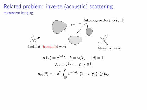
Related problem: inverse (acoustic) scatteringmicrowave imaging
Inhomogeneities (n(x) 6= 1)
Measured waveIncident (harmonic) wave
ui (x) = e ikd·x k = ω/c0, |d | = 1.
∆u + k2nu = 0 in R3.
u∞(θ) = −k2
∫R3
e−ikθ·y (1− n(y))u(y)dy
Inverse problem 1 (parameter identification): Determine n from the knowledgeof u∞ for different incident directions d .
Inverse problem 2 (geometrical problem): Determine D = support(n− 1) fromthe knowledge of u∞ for different incident directions d .

Linearized inverse (acoustic) scatteringultrasound, radar and sonar
Inhomogeneities (n(x) 6= 1)
Measured waveIncident (harmonic) wave
Linearization (Born approximation) when |1− n| 1:
u ' ui inside D = support(n − 1)
⇒ u∞(θ, d) ' −k2
∫R3
e−ik(θ−d)·y (1− n(y))dy
⇒ q = (1− n) 7→ u∞ becomes related to linear integral operators
Inverse problem 3 (tomography): Determine q from the knowledge ofu∞(d ,−d) for different incident directions d and different frequencies k.

Example of applications to microwave mammographyPhD thesis of G. Giorgi (2012)
Set up of the microwave mammography:
This numerical breast phantom (free to download1) is derived by thesegmentation of MRI images of female breasts.
Artificially added tumor (black) of diameter 0.5 cm.
1http://uwcem.ece.wisc.edu/home.htm

Example of applications to mammographyPhD thesis of G. Giorgi (defense, April 2012)
Reconstruction with exact knowledge of the background
Frequency = 2GHz20 emitting/measuring antennas3% of Gaussian noise on the measurements field.
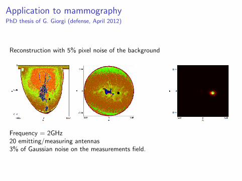
Application to mammographyPhD thesis of G. Giorgi (defense, April 2012)
Reconstruction with 5% pixel noise of the background
Frequency = 2GHz20 emitting/measuring antennas3% of Gaussian noise on the measurements field.

3-D electromagnetic inverse scatteringCollino-Fares-Haddar (2004)
A toy problem: Full aperture measurements of electromagnetic far-field data.Perfectly conducting scatterer.
Exact geometry Reconstruction with λ = 0.225

3-D electromagnetic inverse scatteringCollino-Fares-Haddar (2004)
A toy problem: Full aperture measurements of electromagnetic far-field data.Perfectly conducting scatterer.
Exact geometry Reconstruction with λ = 0.112

3-D electromagnetic inverse scatteringCollino-Fares-Haddar (2004)
A toy problem: Full aperture measurements of electromagnetic far-field data.Perfectly conducting scatterer.
Exact geometry Reconstruction with λ = 0.075

Underwater acoustic imagingArens-Gintides-Lechleiter (2010)
Full aperture measurements of acoustic propagative modes.
Penetrable scatterer. Neumann bdry condition, top. Dirichlet bdry condition,bottom.