Influence of an extended source on Goniopolarimetry (or Direction

Finding) with Cassini and STEREO radio receivers

B. Cecconi

Oct. 23rd, 2006: Accepted for Publication in Radio Science (AGU)

Abstract

In a recent paper, Cecconi and Zarka (2005) provided analytical goniopolarimetric inversions — i.e.which allow us to retrieve the direction of arrival of an incoming electromagnetic wave, its flux, andits polarization state, also referred as direction finding inversions — to be used with measurementsacquired with a system of electric dipole antennas on a three axis stabilized spacecraft such as theCassini/RPWS/HFR or the STEREO/Waves receivers. In the present study, we establish the expressionsof the measurements (auto- and cross-correlations) in the case of an extended source . We also analyzethe effect of an extended source on the outputs of the analytical inversions presented in the former paper,which are supposing a point radio source. We show that for a source with an angular half width smallerthan 5, the induced biases are not significant.

1 Introduction

As the Earth’s ionosphere is reflecting out incoming low frequency radio waves, space based radio experimentsare necessary in the range f ≤ 10 MHz. Constraints on size and mass of embarked antennas impose theuse of simple antennas (monopoles or dipoles) of typical length L ∼ 10 − 50 m. The corresponding spatialresolution of such radio instruments — defined as λ/D, where λ is the observation wavelength and D thetypical aperture of the telescope or radio telescope — is very poor, as λ/L ∼1 or even 1. There is thus noinstantaneous spatial resolution with such antennas. A more adapted description of the antenna directivity isits beaming pattern which gives the antenna gain for each direction of space. The beaming pattern of a shortdipole — the short dipole approximation requires L λ — varies as sin2 θ where θ is the angular distancebetween the source direction and the dipole direction. By integration of the beaming pattern over the wholespace, we get the beaming solid angle, which is 8π/3 sr for a short dipole. This solid angle represents thus2/3 of the 4π sphere. Specific techniques have been derived to retrieve angular resolution from measurementsperformed simultaneously with several (2 or 3) dipoles: these are named Direction–Finding techniques inthe literature. As the determination of the wave vector ~k (direction of arrival of the wave) is coupled withthe determination of the wave polarization (e.g. 2 waves with opposite circular polarization and comingfrom opposite directions give the same signature), I propose to use instead the word Goniopolarimetry (GP),which recalls that we get both direction and polarization of the incoming wave.

Available GP techniques include (i) analysis of the modulations of the signal received by 1 or 2 antennas ona spinning spacecraft [Lecacheux , 1978; Manning and Fainberg , 1980; Ladreiter et al., 1994]; (ii) analysis ofauto- and cross-correlations measured on 2 or 3 antennas on a 3 axis stabilized spacecraft [Lecacheux , 1978;Ladreiter et al., 1995; Vogl et al., 2004; Cecconi and Zarka, 2005].

1

Cecconi and Zarka [2005] (hereafter paper 1) presented a new set of analytical GP techniques, adapted tothe RPWS (Radio and Plasma Wave Science) experiment onboard Cassini [Gurnett et al., 2004]. Due tosimilarity in the receiver design, these same inversion techniques will be used for analysing the data collectedby the radio receivers (Waves) of the two STEREO (Solar TErrestrial RElations Observatory) spacecrafts[Kaiser , 2005].

The GP techniques presented in paper 1 are based on the assumption that the radio source is unresolved.A radio source is considered unresolved when its apparent size is smaller than the spatial resolution of theobserving system. In paper 1, we showed that the derived source position accuracy is of the order of 1− 2

for point source GP. This accuracy is suitable for the Cassini data measured at Saturn, but is insufficientfor STEREO data, as the solar radio bursts have a broad extension as viewed from the orbit of the Earth[Steinberg et al., 1985]. The purpose of this paper is to take into account extended sources. In addition to thewave flux density (I), polarization (Q, U , V ) and direction of arrival (θ, φ), we add here one parameter: thedisk-equivalent radius of the source, which is the radius of the disk-like equivalent source best representingthe real source (the latter being not necessarily a disk). We propose three source modelizations definedby their radial intensity profile: uniform, spherical or gaussian. Any other intensity profile can be studiednumerically.

We evaluate the analytical expressions of the measurements (auto- and cross-correlations) including theangular extension of the source. We also investigate the effect of the source extension on goniopolarimetricresults using point source inversions.

2 Correlation Response to an Extended Source

The analysis below is inspired by Manning and Fainberg [1980], who proposed inversions for Ulysses/URAPmeasurements (spinning spacecraft with a system of two orthogonal antennas, but without cross correlationmeasurements). We extend here their study to radio measurements obtained on a stabilized spacecraftwith a system of antenna with any geometrical configuration. We consider an extended source subtendinga solid angle Ω. All the directions are specified by their colatitude θ and azimuth φ. As we express thetypical extension of the source in terms of its disk-equivalent radius, we will consider an axisymmetricequivalent source and centered on the (θC , φC) direction. The angular disk-equivalent radius is γ so thatΩ = 2π(1 − cos γ). Any point M of the source is defined by its (θM , φM ) direction. Fig. 1 illustratesthese definitions in an adequate coordinate system. All points of the source are considered to have thesame polarization Stokes parameters (Q, U , V ) [Kraus, 1966] (homogeneous source assumption), but weallow a radial flux density S profile. We also consider that the electromagnetic waves coming from eachpoint of the source is phase-decorrelated with the waves coming from the neighboring points of the source(phase-decorrelation assumption).

We consider valid the short antenna hypothesis, i.e. the equivalent dipole effective lengths (L) are shortcompared to the wavelength, i.e. L λ. The effective length of the Cassini/RPWS electrical antennas is8.5m in dipole mode and 7.9m in monopole mode [Zarka et al., 2004], which gives an upper frequency limit∼ 1.5MHz for the validity of the GP analysis. For the STEREO/Waves antennas, the equivalent dipoleeffective lengths have not been measured in-flight at the time of this writing, but Oswald et al. [2006] andRucker et al. [2005] estimated through wire-grid simulations that the upper frequency limit for GP is about∼ 1.5MHz (and stressed upon the need for confirmation by in-flight calibration). The physical antennalength is 6m. Below 1.5 MHz, we can thus assume that each electrical antenna — composed of a monopoleand the spacecraft’s conducting body — is equivalent to a perfect dipole, whose effective parameters (length(h) and direction (θ, φ)) must be carefully calibrated before GP analysis [Vogl et al., 2004,paper 1]. Underthis assumption, the voltage V measured at the antenna’s output is the projection of the wave electric field~E on the effective electrical antenna ~h, i.e. V = ~h. ~E. For an electromagnetic waves, the electric field is

2

φC

θCθM γ

Z

X

YφM

C

hi

M

φi

θi

Ω Z'

Y'

X'

Figure 1: Coordinate system adapted to an axisymmetric source of half viewing angle γ, and centered indirection C (at colatitude θC and azimuth φC). M is the direction of one point of the source. ~hi is thedirection of the ith antenna. The (X, Y, Z) frame is the spacecraft frame. We also represented the sourcecenter reference frame axes (X ′, Y ′, Z ′), which is defined is section 2.2.

represented by a canonical complex function of time: ~E = ~E0 exp(iωt), where ω is the wave pulsation. Theinstantaneous voltage at the antenna’s output is then V = ~E0.~h exp(iωt).

The measurement Pij is the voltage correlation between the antenna i and j outputs and writes Pij =⟨ViV

∗j

⟩,

where Vi and Vj are the voltages measured at antenna i and j outputs respectively, V ∗ is the complexconjugate of V , and 〈· · · 〉 denotes the averaging over an integration time longer than the wave period. Ifi = j, Pii is the autocorrelation of voltages on antenna i, hence a power; if i 6= j, Pij is a cross-correlation.

2.1 Phase-decorrelated source

In the case of point source GP, the expression of the correlation Pij was derived in Ladreiter et al. [1995] andpaper 1. Including explicitly the impedance of free space Z0 and the antenna system gain Ghihj [Manning ,2000] into Pij , we obtain:

Pij = Z0 Ghihj Sij (1)

with:Sij =

S

2[(1 + Q)ΩiΩj + (1−Q)ΨiΨj + (U − iV )ΩiΨj + (U + iV )ΩjΨi

](2)

where Ωn = (~hn. ~Xw)/hn and Ψn = (~hn.~Yw)/hn are the coordinates of the nth antenna unit vector projectedon the wave plane (O, ~Xw, ~Yw) [see Ladreiter et al., 1995, and next section]; the Stokes parameters are: thesource flux density S (in Wm−2 Hz−1), the linear polarization degrees Q and U , and the circular polarizationdegree V . Note that we use the fractional definition of the Stokes parameter polarization degrees — i.e. thetotal received power with e.g. pure circular polarization corresponds to the product S × V . The expressionsof Ωn and Ψn are valid in any reference frame.

In order to study the case of an extended source, we suppose that the source is spatially phase-decorrelated,i.e. that wave packets emitted by each point of the source is phase-decorrelated to the wave packets fromevery other point of the source. The correlation Pij then becomes:

Pij =∫

Ω

dPij (3)

3

(a)

O

C

M1M2

γ

X'Y'

Z'

Xw1

Yw1

Yw2Xw2

θ'2θ'1

(b)

Z'Y'

X'

θ'1

φ'1

φ'2

θ'2

Xw2

Yw2M2 M1

Xw1

Yw1

Figure 2: Reference frame for en extended source: (a) projection on the (OY ′Z ′) plane, (b) polar view. Theextended source reference frame (X ′, Y ′, Z ′) is defined such that the Z ′ axis points towards the center C ofthe extended source. The M1 and M2 directions point to two elementary sources in the extended source. γis the angular half aperture of the source, as seen by an observer placed at the origin O of the frame. TheXwi

and Ywiunit vectors are in the wave plane, perpendicular to the Mi direction (as defined in section

2.2).

with:dPij =

∂Pij

∂ΩdΩ = PΩ

ij dΩ = Z0 Ghihj SΩij dΩ (4)

and:

SΩij =

SΩ

2[(1 + Q)ΩiΩj + (1−Q)ΨiΨj + (U − iV )ΩiΨj + (U + iV )ΩjΨi

](5)

where SΩ is the brightness distribution (in Wm−2 Hz−1 sr−1) over the source. At this point, there is noassumption on source homogeneity, i.e. SΩ, Q, U and V may change across the source.

2.2 Source center frame

We name (X, Y, Z) the spacecraft coordinate system. The source center frame (X ′, Y ′, Z ′) is defined asfollows: Z ′ is pointing towards the center of the source; X ′ is in the (Z,Z ′) plane and its colatitude in the(X, Y, Z) frame is θC + π/2; Y ′ = Z ′ × X ′. In this frame, the angles defining the directions of a point Mof the source are the colatitude θ′M and the azimuth φ′M . The transformation matrix from (X ′, Y ′, Z ′) to(X, Y, Z) is: X

YZ

=

cos θC cos φC − sinφC sin θC cos φC

cos θC sinφC cos φC sin θC sinφC

− sin θC 0 cos θC

X ′

Y ′

Z ′

(6)

Here, X ′ and Y ′ orientation has been defined univocally from the spacecraft coordinate system. Thesevectors can also be defined using specific axes related to the studied source. The transformation matrix isthen different but the results derived remain identical.

For each elementary source Mi, the vectors ~Xwiand ~Ywi

define the wave plane. There is no theoreticalconstraint on the orientation of this pair of vectors, as far as they remain perpendicular to each other [see

4

Ladreiter et al., 1995; Manning and Fainberg , 1980]. The wave frame orientation defines the directions ofthe linear polarization axes. Thus, in order for the linear polarization degrees (Stokes parameters Q and U)to be consistent over a series of observations from various directions in space, the wave frame orientationshould not rotate throughout the source. In the case of an extended source, made of elementary sources Mi,the wave frame must be defined so that all the ~Xwi

vectors are parallel to each other and all the ~Ywivectors

are also parallel to each other. As waves planes are not parallel across the extended source — i.e. the sourcedirections ~Zwi are not colinear — we must to relax the latter constraint: the projections of the vectors ~Ywi

on the (OX ′Y ′) plane — perpendicular to the source center direction — must be parallel as viewed fromthe observer. This condition is illustrated in Fig. 2.

The wave frame vectors in the source center frame (X ′, Y ′, Z ′), ~X ′wi

(θ′i, φ′i), ~Y ′

wi(θ′i, φ

′i) and ~Z ′

wi(θ′i, φ

′i),

depend on θ′i and φ′i. The above condition on the wave frame orientation should then be fulfilled in thevicinity of the Z ′ axis, which is the direction of the source center. In Ladreiter et al. [1995] this condition isnot fulfilled, whereas it is in Manning and Fainberg [1980]. We will thus use the latter definition. We alsouse a reference vector named ~Y0, in order to define the wave frame orientation. The wave frame vectors arethen defined as follows:

~Z ′w =

sin θ′M cos φ′Msin θ′M sinφ′Mcos θ′M

(7)

~Y ′w =

~Z ′w × ( ~Y0 × ~Z ′

w)

|| ~Y0 × ~Z ′w||

(8)

~X ′w = ~Y ′

w × ~Z ′w (9)

Equation (7) means that ~Z ′w points to the source M. Equation (8) defines a unit vector perpendicular to

the line of sight within the (~Y0, ~Z ′w) plane. As equation (8) is only valid if ~Y0 and ~Z ′

w are not colinear, theorientation of ~Y0 has to be carefully chosen depending on the source direction and on the object studied: inthe case of planetary radio emissions, the vector ~Y0 can be defined as the orientation of the magnetic axis ofthe studied planet; for solar corona radio bursts, ~Y0 can be taken perpendicular to the ecliptic plane.

For the ease of further computation, we choose ~Y0 = ~Y ′, as in Manning and Fainberg [1980]. Then:

~X ′w =

1√1− sin2 θ′M sin2 φ′M

cos θ′M0− sin θ′M cos φ′M

(10)

~Y ′w =

1√1− sin2 θ′M sin2 φ′M

− sin2 θ′M cos φ′M sinφ′M1− sin2 θ′M sin2 φ′M− sin θ′M cos θ′M sinφ′M

(11)

Going back in the spacecraft frame (X, Y, Z) using equation (6), we obtain:

~Xw =1√

1− sin2 θ′M sin2 φ′M

cos θC cos φC cos θ′M − sin θC cos φC sin θ′M cos φ′Mcos θC sinφC cos θ′M − sin θC sinφC sin θ′M cos φ′M− sin θC cos θ′M − cos θC sin θ′M cos φ′M

(12)

~Yw =1√

1− sin2 θ′M sin2 φ′M

×

− cos θC cos φC sin2 θ′M cos φ′M sinφ′M − sinφC(1− sin2 θ′M sin2 φ′M )− sin θC cos φC sin θ′M cos θ′M sinφ′M− cos θC sinφC sin2 θ′M cos φ′M sinφ′M + cos φC(1− sin2 θ′M sin2 φ′M )− sin θC sinφC sin θ′M cos θ′M sinφ′M+sin θC sinφC sin2 θ′M cos φ′M sinφ′M − cos θC sin θ′M cos θ′M sinφ′M

(13)

5

Expressions of Ωi = (~hi. ~Xw)/hi and Ψi = (~hi.~Yw)/hi are thus:

Ωi =1√

1− sin2 θ′M sin2 φ′M

[cos θ′M

(sin θC cos θi − sin θi cos θC cos(φC − φi)

)− sin θ′M cos φ′M

(cos θC cos θi + sin θi sin θC cos(φC − φi)

)](14)

Ψi =1√

1− sin2 θ′M sin2 φ′M

[− (1− sin2 θ′M sin2 φ′M ) sin θi sin(φC − φi)

+ sin2 θ′M cos φ′M sinφ′M(cos θi sin θC − sin θi cos θC cos(φC − φi)

)− sin θ′M cos θ′M sinφ′M

(cos θC cos θi + sin θi sin θC cos(φC − φi)

)](15)

2.3 Spatial integration

We define the following useful quantities:

Ai(θC , φC) = − sin θi cos θC cos(φC − φi) + cos θi sin θC (16)Bi(θC , φC) = − sin θi sin(φC − φi) (17)Ci(θC , φC) = sin θi sin θC cos(φC − φi) + cos θi cos θC (18)

This allows us to rewrite Ωi and Ψi as:

Ωi =Ai(θC , φC) cos θ′M − Ci(θC , φC) sin θ′M cos φ′M√

1− sin2 θ′M sin2 φ′M

(19)

Ψi =1√

1− sin2 θ′M sin2 φ′M

(Ai(θC , φC) sin2 θ′M cos φ′M sinφ′M

+Bi(θC , φC)(1− sin2 θ′M sin2 φ′M )− Ci(θC , φC) sin θ′M cos θ′M sinφ′M)

(20)

Each term of equation (5) has then to be integrated over the extended source solid angle using the expressionsΩi and Ψi given in equations (19) and (20). As the source is axisymmetric, the integrations intervals are[0, 2π] for φ′M and [0, γ] for θ′M , with γ ≤ π/2. The voltage correlation Pij then writes:

Pij =Z0 Ghihj

2

2π∫φ′

M=0

γ∫θ′

M=0

SΩ(θ′M , φ′M )×

[(1 + Q)Ωi(θC , φC , θ′M , φ′M )Ωj(θC , φC , θ′M , φ′M )

+(U − iV )Ωi(θC , φC , θ′M , φ′M )Ψj(θC , φC , θ′M , φ′M )+(U + iV )Ωj(θC , φC , θ′M , φ′M )Ψi(θC , φC , θ′M , φ′M )

+(1−Q)Ψi(θC , φC , θ′M , φ′M )Ψj(θC , φC , θ′M , φ′M )]sin θ′Mdθ′Mdφ′M (21)

As the three cases studied below have circular symmetry, integration over φ′M can be performed first. Useful

6

integrals for this first integration step are:∫ 2π

0

dφ′M = 2π, (22)∫ 2π

0

dφ′M1− sin2 θ′M sin2 φ′M

= 2π1

cos θ′M, (23)∫ 2π

0

cos φ′Mdφ′M1− sin2 θ′M sin2 φ′M

= 0, (24)∫ 2π

0

sinφ′Mdφ′M1− sin2 θ′M sin2 φ′M

= 0, (25)∫ 2π

0

cos φ′M sinφ′Mdφ′M1− sin2 θ′M sin2 φ′M

= 0, (26)∫ 2π

0

sin 3φ′Mdφ′M1− sin2 θ′M sin2 φ′M

= 0, (27)∫ 2π

0

cos2 φ′Mdφ′M1− sin2 θ′M sin2 φ′M

= 2π1− cos θ′M

sin2 θ′M, (28)∫ 2π

0

cos2 φ′M sin2 φ′Mdφ′M1− sin2 θ′M sin2 φ′M

= 2π1− cos θ′M − 1/2 sin2 θ′M

sin4 θ′M(29)

Allowing the source brightness distribution to vary radially SΩ = SΩ(θ′M ), but assuming that the polarizationstate is constant all over the source, equation (21) then rewrites:

Pij =∫ γ

0

2π Z0 Ghihj SΩ(θ′M )2

[(1 + Q)

[(AiAj cos θ′M + CiCj(1− cos θ′M )

]+(U − iV )

[AiBj cos θ′M

]+ (U + iV )

[AjBi cos θ′M

]+(1−Q)

[AiAj(1− 2 cos θ′M + cos2 θ′M )/2 + BiBj(1 + cos2 θ′M )/2

+CiCj(1− cos θ′M ) cos θ′M]]

sin θ′Mdθ′M (30)

We define Γk as:

Γk =2π

Ω

∫θ′

M

SΩ(θ′M )SΩ

0

sin(kθ′M )dθ′M (31)

with k ∈ 1, 2, 3 and SΩ0 = SΩ(θ′M = 0). The coefficients Γk are normalized by the total viewing solid angle

of the source Ω in order to be independent of the size of the source. Equation (30) can be simplified usingthe notation Γk and the trigonometric identities:

2 cos θ′M sin θ′M = sin(2θ′M ), 4 cos2 θ′M sin θ′M = sin(3θ′M ) + sin θ′M (32)

The correlation is finally:

Pij =Z0 Ghihj S0

2

[(1 + Q)

(AiAj

Γ2

2+ CiCj

(Γ1 −

Γ2

2

))+(U − iV )

(AiBj

Γ2

2

)+ (U + iV )

(AjBi

Γ2

2

)+(1−Q)

(AiAj

12

(Γ1 − Γ2 +

Γ3 + Γ1

4

)+ BiBj

12

(Γ1 +

Γ3 + Γ1

4

)+CiCj

(Γ2

2− Γ3 + Γ1

4

))](33)

where S0 = SΩ0 Ω, i.e. the total flux density of an equivalent source with an uniform SΩ

0 brightness distribution,subtending a solid angle Ω.

7

S0Ω

−γ γ −γ γ −γ γ

S0ΩS0

Ω(a) (c)(b)

Figure 3: Radial cuts of the three source brightness distributions studied in this paper: (a) uniform source,(b) spherical source and (c) gaussian source.

2.4 Models for radial intensity profiles

We consider hereafter three models for the radial intensity source profiles, all with constant polarization (Q,U , V ) across the source. The only parameter that may change across the source is the brightness distributionSΩ, but with circular symmetry along the direction of the source center. The three cases studied (illustratedin Fig. 3) are (a) a uniform source with radius γ:

SΩa (θ′M ) = SΩ

0 , (34)

(b) a spherical source of radius γ with an optically thin surface:

SΩb (θ′M ) = KbS

Ω0

√1−

tan2 θ′Mtan2 γ

, (35)

and (c) a gaussian source with a 2γ full width at half maximum:

SΩc (θ′M ) = KcS

Ω0 exp(− ln(2) tan2 θ′M/ tan2 γ). (36)

The coefficients Kb and Kc are normalization coefficients ensuring consistency with point source results (asdescribed in paper 1).

2.4.1 Case of a uniform source

With a brightness profile SΩa (θ′M ) being simply SΩ

0 for θ′M < γ and 0 outside, Γak is then:

Γak(γ) =

11− cos γ

∫ γ

0

sin(kθ′M )dθ′M =1− cos(kγ)k(1− cos γ)

(37)

for k ∈ 1, 2, 3. Each term Γak(γ) can be simplified, leading to:

Γa1(γ) = 1, Γa

2(γ) = 1 + cos γ, Γa3(γ) =

43(1 + cos γ + cos2 γ)− 1 (38)

Computing the value of Γak when γ → 0 allows us to check that the measured power is consistent with the

one measured in case of a point source [Ladreiter et al., 1995,paper 1]. We have:

limγ→0

Γak(γ) = k (39)

8

This gives us the following correlation for γ = 0:

Pij =Z0 Ghihj S0

2[(1 + Q)AiAj + (U − iV )AiBj + (U + iV )AjBi + (1−Q)BiBj ] (40)

As Ai(θC , φC) = Ωi(θC , φC , 0, 0) and Bi(θC , φC) = Ψj(θC , φC , 0, 0), equation (40) is exactly the expressionof the measurement induced by a point source located along the (θC , φC) direction, with Stokes parametersS0, Q, U , V .

2.4.2 Case of a spherical source with an optically thin surface

The brightness profile is varying radially as SΩb (θ′M ) given by equation (35). Γb

k then writes:

Γbk(γ) =

Kb

1− cos γ

∫ γ

0

(1− tan2 θ′M

tan2 γ

)1/2

sin(kθ′M )dθ′M (41)

When the source is small (γ π/2), we have tan(γ) ∼ γ. As 0 < θ′M < γ, we also have tan θ′M ∼ θ′M andsin(kθ′M ) ∼ kθ′M . It is then easy to show that at the point source limit (γ → 0), Γb

k becomes:

limγ→0

Γbk(γ) =

3kKb

2(42)

Setting Kb = 2/3, we ensure consistency with the uniform source model (a) and the limit case of a pointsource.

2.4.3 Case of a gaussian source

We consider here a source that has a gaussian brightness radial profile SΩc (θ′M ) given by equation (36). Γc

k

is then:

Γck(γ) =

Kc

1− cos γ

∫ π/2

0

exp(− ln(2)

tan2 θ′Mtan2 γ

)sin(kθ′M )dθ′M (43)

When the source is small (γ π/2), we have tan(γ) ∼ γ. The same approximation applies to tan θ′M onlywhen 0 < θ′M < γ. However, we use here this approximation from 0 to π/2, but inside an exponentialfunction. Fig. 4 shows that this approximation is valid for all sizes of sources. Γc

k then rewrites:

Γck(γ) =

Kc

1− cos γ

∫ π/2

0

exp(−θ′M

2

ξ2

)sin(kθ′M )dθ′M (44)

with ξ = γ(ln 2)−1/2 and k ∈ 1, 2, 3. The limit of Γck when γ → 0 is:

limγ→0

Γck(γ) =

kKc

ln 2(45)

Setting Kc = ln 2, we ensure consistency with the uniform source model (a) and the limit case of a pointsource.

We can redefine the coefficients Γbk(γ) and Γc

k(γ) including the above multiplying factors. We will thus use:

Γbk(γ) =

23

11− cos γ

∫ γ

0

SΩb (θ′M ) sin(kθ′M )dθ′M (46)

Γck(γ) =

ln 21− cos γ

∫ γ

0

SΩc (θ′M ) sin(kθ′M )dθ′M . (47)

The numerical values for coefficients Γmk (γ) (with or without the small source approximation in models (b)

and (c)), computed using a Romberg integration method, are shown in Fig. 4.

9

Γ 1a (γ)

Γ 2a (γ)

0.0

0.5

1.0

1.5

2.0

2.5

3.0

Γ 3a (γ)

0.0

0.5

1.0

1.5

2.0

2.5

3.0

0 20 40 60 800 20 40 60 80

0 20 40 60 80 0 20 40 60 80

0 20 40 60 800 20 40 60 80

0 20 40 60 80

0 20 40 60 80

0 20 40 60 80

0.0

0.5

1.0

1.5

2.0

2.5

3.0

0.0

0.5

1.0

1.5

2.0

2.5

3.0

0.0

0.5

1.0

1.5

2.0

2.5

3.0

0.0

0.5

1.0

1.5

2.0

2.5

3.0

0.0

0.5

1.0

1.5

2.0

2.5

3.0

0.0

0.5

1.0

1.5

2.0

2.5

3.0

0.0

0.5

1.0

1.5

2.0

2.5

3.0

Source Half Width Angle (γ) [deg]

Uniform Brightness Source Profile Spherical Brightness Source Profile Gaussian Brightness Source Profile

Source Half Width Angle (γ) [deg] Source Half Width Angle (γ) [deg]

Nu

mer

ical

Val

ue

Nu

mer

ical

Val

ue

Nu

mer

ical

Val

ue

Γ 1c (γ)

Γ 2c (γ)

Γ 3c (γ)

Γ 1b (γ)

Γ 2b (γ)

Γ 3b (γ)

Figure 4: Normalized Γmk coefficient as a function of the source half viewing width (γ). Coefficients for

model (a), (b) and (c) are respectively shown in the 1st, 2nd and 3rd column. Coefficients of order k = 1, 2and 3 are shown in row 1, 2 and 3, respectively. The coefficients were computed using the expressions with(dashed line, only for model (b) and (c)) or without (solid line) of small source approximation.

10

3 Errors induced by the source extension on GP results

Equation (33) gives the expression of the measurements recorded with dipole antennas in the case of anextended source with circular symmetry. We use below these expressions to evaluate the influence of thesource size and radial profile on GP inversions that are assuming unresolved radio sources.

We study two GP inversions presented in paper 1. The “General Case Inversion”, for which there is noassumption on the source (except that it is unresolved), is valid for V 6= 0. The “Circular polarization CaseInversion” is dedicated to sources with no linear polarization. For that second inversion, the case V = 0 isnot singular. Both inversions require simultaneous measurements on three non coplanar antennas.

Following the method of paper 1, we simulate the receiver response induced by an extended source — i.e.using eq. (33) to model the measurements — and assume that these measurements were obtained with apoint source (as in eq. 2) for the GP inversion. We test several source center directions in the spacecraftframe and several polarization states. As the flux density only appears as a multiplying factor for correlationmeasurements, we simulate our data with a single value S0 = 10−15Wm−2 Hz−1. We use the model antennaparameters used in paper 1, which are close to the actual ones of the Cassini/RPWS electrical antennasystem. The three antennas are named ~h+X , ~h−X and ~hZ . Their effective relative length, colatitude andazimuth in the spacecraft frame, are respectively: h+X = 1.0, θ+X = 110 and φ+X = 20; h−X = 1.0,θ−X = 115 and φ−X = 165; hZ = 0.8, θZ = 30 and φZ = 90.

As in paper 1, we define β+XZ (resp. β−XZ) as the angular distance between the source direction and theplane formed by the ~h+X (resp. ~h−X) and ~hZ pair of antenna, and αZ as the angular distance between thesource direction and the ~hZ antenna.

3.1 General Case Inversion

This inversion (see paper 1, section 2.1.1) uses three antenna measurements and solves for the full set ofGP unknowns (S, Q, U , V , θ and φ). We have shown in paper 1 that the data selection necessary toget accurate measurements with this inversion is a Signal to Noise Ratio (SNR>23 dB) coupled with ageometrical selection β±XZ > 20, which also implies αZ > 20. With these constraints, we achieve anaccuracy of 1 on directions, 1 dB on flux densities and 10% on polarization measurements.

The simulation data sets were built with 2522 source directions (5 steps in azimuths and colatitudes) and208 polarization states (excluding V = 0). Each run is computed with one of the three source profile models(a, b or c) and a given source size γ (1, 2, 5 or 10). This gives thus a total of 2522 × 208 = 524576simulated data points for each of the 12 (= 3× 4) runs.

The error levels are summarized in Table 1.

3.1.1 Source position determination

The GP inversion provides the colatitude θ and azimuth φ defining the direction of arrival of the incomingelectromagnetic wave in the spacecraft frame. We define the error on the source determination as the angulardistance between the true direction of the center of the simulated source (input values) and the resultingvalue given by the GP inversion (output values). This angular distance is noted ∆ξ.

11

Angular error (∆ξ) with γ=5° (uniform source profile)

20

20

cola

titu

de

θ [d

eg in

SC

fram

e]

azimuth φ [deg in SC frame]

hz

h+xh–x

00

50

100

150

100 200 300

1 11

1

1

1

1

12

2

5

5

10

2

2

2

2 2

2

1

1 1

1

1

2

2

22

2

5

5

510

2

2

Figure 5: Angular Error on GP results using the “General Case Inversion”, for an extended source with aγ = 5 and an uniform brightness profile (model a). Isocontour lines are represented in the spacecraft framespherical coordinates: colatitude θ and azimuth φ. The antenna directions are marked with + signs andlabelled as in paper 1. The different isocontour lines are: mean angular error for a given direction (solidline); maximum angular error for a given direction (doted line); 20 distance from the hZ antenna (thickdashed line + shaded region).

Fig. 5 displays the angular bias induced by an extended source with γ = 5 with a uniform intensity profile(model a). The errors are deterministic and depend on both direction of arrival and polarization degree.The condition αZ > 20 is consistent with a ∼1 average error and a ∼5 maximum error.

Fig. 6 summarizes the same results for different source angular half widths (γ = 1, 2, 5 and 10). We havedisplayed the error probability levels on the source position. A 1% (50%, resp.) error probability level meansthat only 1% (50% resp.) of the simulated data points have an error greater than this value with the givenangular selection threshold and the given source profile and angular width. Fig. 7 shows the same databut displaying the spherical (and gaussian) source profile error probability levels versus the uniform sourceprofile error probability levels. This Fig. clearly shows that the error induced by a spherical profile sourcewith an angular half width γ is equal to the one induced by a uniform profile source with an angular halfwidth 0.80γ. The same statement can also be done with the gaussian profile source, equivalent to a 2.88times larger uniform source profile. Comparing the actual angular biaises induced by the different modelson the simulation grid, we observe that this also means that a spherical (or gaussian) profile source inducesthe same amount of angular bias on the source position as a uniform profile source with an angular widthlarger by the given factor.

3.1.2 Source polarization determination

The GP inversion provides the polarization state of the detected incoming electromagnetic wave in termsof two sets of three Stokes parameters (Q, U , V ). Each set is computed using either the (h+X ,hZ) pair ofantennas or the (h−X ,hZ) one. We only show the results obtained on the (h+X ,hZ) pair of antennas. We

12

10

1

20 40 60 800

0.1

0.01

An

gu

lar E

rro

r ∆ξ

(deg

ree)

αz (degree)

50% – γ =10°

1% – γ =10°

1% – γ =5°

1% – γ =2°

50% – γ =5°1% – γ =1°50% – γ =2°

1% and 50% Error probability levels for Angular error (∆ξ) (uniform source profile)

Figure 6: Error probability levels on the source position ∆ξ caused by an extended source using the “GeneralCase Inversion”. The error probability levels 1% and 50% are displayed versus the angular selection thresholdαZ , for an uniform brightness source (model a), and for several source angular width γ = 1, 2, 5 or 10.

1% probability angular errors 50% probability angular errors

10

10

1

1

0.1

0.10.01

0.01

An

gu

lar E

rro

r (d

eg)

Angular Error (deg) [uniform]

1010.10.01

Angular Error (deg) [uniform]

10

1

0.1

0.01

γ=1°

γ=2°

γ=5°

γ=10°

gaussian

spherical

uniform

Caption

Source size

Source profile

Figure 7: Comparison of the angular errors induced by the three different source profiles, for several angularthresholds and for two error probability levels (left: 50%, right: 1%). We used the angular error levelsdisplayed in figure 6 and displayed the gaussian and spherical source profile results versus the uniform sourceprofile ones. We observe that the error probability levels induced by a spherical (resp. gaussian) brightnessdistribution model is equivalent to the error probability levels induced by an uniform brightness distributionmodel with a radius 0.80γ (resp. 2.88γ).

13

Error on Circular Polarization Degree (∆V) with γ=5° (uniform source profile)

cola

titu

de

θ [d

eg in

SC

fram

e]

azimuth φ [deg in SC frame]0

0

50

100

150

100 200 300

0.01

0.10

0.01

0.01

0.10

0.1010

10

10

10

10

10

10

0.50

0.50

0.50

0.50

0.50

0.50

0.50

0.10

0.100.10

0.100.10

0.10

0.10

0.10

100.50

0.10

0.10

0.10

0.01

0.01

0.01

0.01

0.01

0.01

0.10

0.01

0.01

0.01

0.01

0.01

h–xh+x

hz

Figure 8: Circular polarization error on GP results using the “General Case Inversion”, for an extendedsource with a γ = 5, an uniform brightness profile (model a) and for the (h+X ,hZ) pair of antennas.Isocontour lines are represented in the spacecraft frame spherical coordinates: colatitude θ and azimuth φ.The antenna directions are marked with + signs and labelled as in paper 1. The different isocontour linesare: mean angular error for a given direction (solid line); maximum angular error for a given direction (dotedline); 10 distance from the (h+X ,hZ) pair of antenna plane (thick dashed line).

show first the error on the circular polarization degree, noted ∆V , which is the absolute difference betweenthe circular polarization degrees of the simulated incoming wave and the resulting value computed throughthe inversion. We then show the error on the linear polarization degree, noted ∆L, with L =

√Q2 + U2.

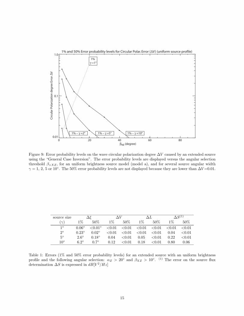
Fig. 8 shows the error on the circular polarization degree induced by a extended source with γ = 5 witha uniform intensity profile (model a). The β+XZ > 10 condition is consistent with a .10% average (andmaximum) error. A β+XZ > 20 geometrical condition would be consistent for a ∼1% average accuracy.Fig. 9 summarizes the same results for different angular source widths (γ = 1, 2, 5 and 10). This figureis interpreted as in Fig. 6 (see section 3.1.1). This figure shows that the absolute error on the circularpolarization degree (1% error probability level) is typically less than 0.10 for βXZ>10 with γ = 5.

The same analysis has been done for the errors on the linear polarization degree (∆L) and the results arevery similar: the absolute error on the circular polarization degree (1% error probability level) is less than0.10 for βXZ>7.5 with γ = 5. The 50% error probability level drops below 0.01 for βXZ>7.5, withγ = 10.

3.1.3 Source flux determination

The error on the source flux determination (∆S) are expressed in dB[V 2/Hz], i.e. as a log scaled spectralpower. The variations of ∆S are similar to the one presented on Fig. 8. Using the geometrical selectionβXZ>10 with γ = 5, the 50% error probability level is 0.22 dB[V 2/Hz], and the 1% level is below 0.01dB[V 2/Hz].

14

1.0

20 40 60 800

0.1

0.01

Cir

cula

r Po

lari

zati

on

deg

ree

Erro

r ∆V

βxz (degree)

1% – γ =10°1% – γ =5°1% – γ =2°

1% and 50% Error probability levels for Circular Polar. Error (∆V) (uniform source profile)

1% γ =1°

Figure 9: Error probability levels on the wave circular polarization degree ∆V caused by an extended sourceusing the “General Case Inversion”. The error probability levels are displayed versus the angular selectionthreshold β+XZ , for an uniform brightness source model (model a), and for several source angular widthγ = 1, 2, 5 or 10. The 50% error probability levels are not displayed because they are lower than ∆V =0.01.

source size ∆ξ ∆V ∆L ∆S(1)

(γ) 1% 50% 1% 50% 1% 50% 1% 50%1 0.06 <0.01 <0.01 <0.01 <0.01 <0.01 <0.01 <0.012 0.23 0.02 <0.01 <0.01 <0.01 <0.01 0.04 <0.015 2.6 0.18 0.04 <0.01 0.05 <0.01 0.22 <0.0110 6.2 0.7 0.12 <0.01 0.18 <0.01 0.80 0.06

Table 1: Errors (1% and 50% error probability levels) for an extended source with an uniform brightnessprofile and the following angular selection: αZ > 20 and βXZ > 10. (1) The error on the source fluxdetermination ∆S is expressed in dB[V 2/Hz]

15

3.1.4 Final data selection

Table 1 summarizes the errors for different source sizes with an angular selection αZ > 20 and βXZ > 10.This angular selection includes the selection given in paper 1, which was βXZ > 20. This latter criterionis required to get the following typical errors in case of a point source: ∆ξ < 1, ∆S < 1.0dB, ∆L < 0.1and ∆V < 0.1. The angular selection obtained in this study is providing the same order of magnitude ofaccuracy for flux and polarization parameters (∆S, ∆L and ∆V ) with a source half aperture γ < 10, andfor direction of arrival determinations with a source half aperture γ < 5. As noted in Fig. 7 (and observedfor ∆S, ∆V and ∆L also), the source profile only changes the error levels with a scaling factor supposingthat a gaussian profile source is equivalent to the 2.88 (0.80 in case of a spherical source) times larger uniformsource.

3.2 Circular Polarization Case Inversion

This inversion (see section 2.1.2 in paper 1) uses the three antenna measurements to solve the GP equations incase of a incoming wave that has no linear polarization (U=Q=0). The unknowns are then S, V , θ and φ. Weshowed in paper 1 that the data selection necessary to get accurate measurements with this inversion is a SNRselection (SNR>23 dB) coupled with a geometrical selection β±XZ > 20. A second geometrical selectionwas pointed out: αZ < 50 taking into account the 8-bits digitization errors (as for the Cassini/RPWS radioreceiver). In the case of a 12-bits digitalization scheme (as for the two STEREO/Waves radio receivers),this last selection is not useful. With the data selection mentioned, we can achieve an accuracy of 1 ondirections, 1 dB on flux measurements and 10% on polarization measurements.

The simulation data sets was built with 9 circular polarization states (between −1 and 1, with 0.25-widesteps) and 10226 directions of arrival (2.5 steps in azimuths and colatitudes). Each run is computed withone of the three source profile models (a, b or c) and a given source size γ (1, 2, 5 or 10). This givesthus a total of 9× 10226 = 92034 simulated data points for each of the 12 (= 3× 4) runs.

3.2.1 Source position determination

As in section 3.1.1, we characterize the errors with ∆ξ. Fig. 10 shows error level isocontours for the “CircularPolarization Case Inversion”. The figure shows that the errors are larger along the antenna planes: mainlyalong the (h±X ,hZ) planes and in a smaller extent along the (h+X ,h−X) plane. With βXZ > 10, the 1%angular error probability level is lower than 2 for γ < 5, and the 50% error probability level is lower than1 for γ < 10. With a more restricted angular selection (βXZ > 22), we get ∆ξ lower than ∼ 1 for γ < 10

(at the 1% error probability level). Note that the latter selection is removing the area situated between the(+X, Z) and (−X, Z) antenna planes where the error amplitudes are higher (see Fig. 10).

3.2.2 Source polarization determination

We are supposing here that the source has no linear polarization (i.e. Q=0 and U=0). The circular polar-ization error on GP results using this inversion is similar to the ones presented on Fig. 8 for the general caseinversion. With βXZ > 10, the 1% error probability level is lower than 0.12 for any γ < 10.

16

Angular error (∆ξ) with γ=5° (uniform source profile)

cola

titu

de

θ [d

eg in

SC

fram

e]

azimuth φ [deg in SC frame]

hz

h+x h–x

00

50

100

150

100 200 3001

2

2

10

2

2

11

2

2

2

22

2

2

2

21

1

1

2

10

5

1

11

1

5

21

1

2

1

1

5

Figure 10: Angular Error on GP results using the “Circular Polarization Inversion”, for an extended sourcewith a γ = 5 and an uniform brightness profile (model a). Isocontour lines are represented in the spacecraftframe spherical coordinates: colatitude θ and azimuth φ. The antenna directions are marked with + signsand labelled as in paper 1. The solid lines are maximum angular error isocontours for a given direction.The thick dashed lines show the direction within the antenna planes (hZ and h±X); these set of directionscorrespond to β±XZ = 0. The thick dotted line is the direction perpendicular to the hZ antenna (αZ = 90).

17

Flux error (∆S) in dB[V2/Hz] with γ=5° (uniform source profile)

cola

titu

de

θ [d

eg in

SC

fram

e]

azimuth φ [deg in SC frame]0

0

50

100

150

100 200 300

–0.1

–0.1

–0.1

–0.1

–0.1

–0.1

0.1

–0.1

0.1

0.1

0.5

0.5

0.51.0

1.0

0.00.0

0.0

0.0

0.0

0.0

0.1

h–xh+x

hz

Figure 11: Flux Error on GP results using the “Circular Polarization Inversion”, for an extended source witha γ = 5 and an uniform brightness profile (model a). Flux density errors are in dB[V 2/Hz]. Isocontourlines are represented in the spacecraft frame spherical coordinates: colatitude θ and azimuth φ. The antennadirections are marked with + signs and labelled as in paper 1. The solid lines are maximum angular errorisocontours for a given direction. The thick dashed lines show the direction within the antenna planes (i.e.the directions corresponding to β±XZ = 0). The grey shaded areas correspond to the positive error areas(measured flux greater than actual flux), the white ones are the negative ones.

18

source size ∆ξ ∆V ∆S(1)

(γ) 1% 50% 1% 50% 1% 50%1 <0.1 <0.1 <0.01 <0.01 <0.01 <0.012 0.3 <0.1 <0.01 <0.01 0.03 <0.015 2.0 0.2 0.04 <0.01 0.19 0.0110 7.1 0.9 0.12 <0.01 0.66 0.03

Table 2: Typical errors (1% and 50% error probability levels) for an extended source with an uniformbrightness profile and an angular selection βXZ > 10. (1) The error on the source flux determination ∆S isexpressed in dB[V 2/Hz]

3.2.3 Source flux determination

The error on the flux determination are shown on Fig. 11 for γ = 5 and a uniform source profile. Thisfigure shows that strong errors occur along the antenna planes — i.e. the planes (hZ ,h+X) and (hZ ,h−X)— and close to the hZ antenna direction. With 10, we restrict the error levels below ∆S > 1dB[V 2/Hz].Table 2 shows the 1% and 50% error probability levels.

3.2.4 Final data selection

Table 2 summarizes the error levels for different source sizes with a typical angular selection βXZ > 10.This angular selection is less constraining than the selection given in paper 1, which was βXZ > 20 andαZ < 50. This latter criterium is required to get the following typical errors in case of a point source:∆ξ < 1, ∆S < 1.0dB and ∆V < 0.1. The angular selection obtained in this study is providing the sameorder of magnitude of accuracy for flux and polarization parameters (∆S, ∆L and ∆V ) with a source halfaperture γ < 10, and for direction of arrival determinations with a source half aperture γ < 5.

4 Discussion

We have obtained the expressions of measurements (auto- and cross-correlation of the voltages measured ontwo antennas) taking into account the size of the source with different radial brightness distribution profiles,given its disk-equivalent radius. The general expression is proposed in Eq. (33). We have checked that in caseof γ = 0 the expressions are identical to the ones published in previous studies [Lecacheux , 1978; Ladreiteret al., 1995,paper 1]. We also checked expression (33) against the previous results on extended source GPpublished by Manning and Fainberg [1980]. Although their formulas were obtained in a special case (auto-correlation only with perpendicular antennas on a spinning spacecraft), we obtain the same expressions (seeappendix A). The expressions have been formulated here for three different radial intensity profiles (uniform,spherical and gaussian). Any other radial intensity profile can be studied numerically.

We have studied in this paper the case of an axisymmetric source, assuming that any extended source couldbe represented by its disk-equivalent source. We numerically computed the correlation response for ellipticalsources with uniform brightness and polarization degrees distributions. This study allowed us to check thatan uniform elliptical source induce the same voltage correlation than the uniform circular source whichsubtends the same solid angle, ensuring the validity of our assumption.

We have shown that the errors on the results of the analytical GP inversions presented in paper 1 are within

19

the error bars of these inversions, given a geometrical selection (which includes the geometrical selectionproposed in paper 1) and a disk-equivalent radius of the source below 5 for directions and 10 for flux andpolarization. The error levels are given in Tables 1 and 2. As shown in Fig. 7, the radial intensity profileof the source only modifies the amplitude of the final error on GP with a scaling factor: a gaussian source(resp. spherical) induces errors equivalent to a 2.88 (resp. 0.80) times larger uniform source. Any othersource profile might be studied but they are likely to show the same behaviour.

The implications of this study on the scientific results obtained with point source inversions are differentdepending on the observed source. In the case of the Saturn (observed with Cassini), the closest Saturnflyby of Cassini occurred during the insertion orbit at ∼1.3 RS (Saturn radii, 1 RS=60,268 km). At thisdistance a 5 source is approximately 6800 km (0.11RS). There is no estimate of the size of the radio sourcesat Saturn. Cowley et al. [2004] gave an estimation for the width of the UV aurora active region at Saturn of500–1000 km width. This gives the typical width the region in which the auroral radio emission may occur.However the radio emission beaming pattern is not isotropic but probably has the shape of a hollow cone[Zarka, 1998]. The radio emission are also very bursty and sporadic. It is then unlikely that a spacecraftwill be within the emission beam of several contiguous sources. The point source hypothesis is thus valid inthe case of Saturn’s auroral radio emissions. In the case of solar radio bursts, Steinberg et al. [1985] showedthat the typical angular extension of type III bursts is of the order of 30 at 100 kHz when observed fromthe Earth. This angular extension is induced by scattering. The point source GP inversions may then giveerroneous results. A GP inversion providing the size of the source thus is necessary to characterize correctlythe solar radio bursts with the STEREO/Waves experiments.

A full GP inversion providing the size of the source requires the inversion of the GP measurements system fordirections (θ, φ), flux (S), polarization (Q, U , V ) and disk-equivalent radius of the source (γ), i.e. invertinga system of 7 (3 auto- and 2 complex cross-correlations, as for the Cassini data) or 9 (3 auto- and 3 complexcross-correlations, as for the STEREO data) measurements for 7 unknowns. As the system is degenerated —it is not possible to obtain separately direction and polarization, see paper 1 — it might not be possible toobtain the full set of GP unknowns as a result in the case where we have only 7 measurements. Assumptionson different parameters would however help inverting the system in that case (for instance: giving the positionof the source center or supposing that the source has no polarization or is purely circularly polarized). Thismeans that only the STEREO data might be able to be used to do full GP inversions including the sizeof the source. If no analytical direct inversion is found, it may be built on a minimization process [seeLadreiter et al., 1995; Santolık et al., 2003; Vogl et al., 2004] and will be described in a future paper. Thepresent study however characterize the limits of the GP inversions derived in paper 1 in case of an extendedradio source. Finally, this study can also be used for the future JUNO mission (jovian polar orbiter withperijoves < 5000km). If this spinning spacecraft has a GP radio receiver onboard, it will provide radio sourcelocalization with an accuracy of a few 100 km, close to that obtained with the UV images from the HubbleSpace Telescope (1 pixel is about 200 km).

Acknowledgement

The author was supported by the CNES (Centre National d’Etudes Spatiales) through a Post-Doctoral fel-lowship. The author would like to thank P. Zarka, M. Maksimovic and S. Hoang for their helpful suggestionsand discussions, as well as Jean-Louis Bougeret, Principal Investigator of the STEREO/Waves experiment.

20

A Checking equation (33) with Manning and Fainberg [1980] re-sults

Manning and Fainberg [1980] provided an equation set to solve the problem in the particular case of aspinning spacecraft. In addition the two antennas considered were supposed to be either axial (θ// = 0) orequatorial (θ⊥ = π/2) and they only computed the spectral power on one antenna at a time (autocorrelationonly). Our expressions are valid whatever the antenna direction is. We check here their consistency withManning and Fainberg [1980] ones.

Equation (33) gives us the general expression of the spectral power measured by dipole antennas in the caseof an extended source. As Manning and Fainberg [1980] made the assumption that the source was uniform,we can rewrite equation (33) using model a, in the case of the autocorrelation on the ith antenna:

Pii =Z0 Gh2

i S0

2

[(1 + Q)

(A2

i

1 + cos γ

2+ C2

i

1− cos γ

2

)+ 2U

(AiBi

1 + cos γ

2

)+(1−Q)

(A2

i

12

(− cos γ +

1 + cos γ + cos2 γ

3

)+B2

i

12

(1 +

1 + cos γ + cos2 γ

3

)+C2

i

(1 + cos γ

2− 1 + cos γ + cos2 γ

3

))](48)

In the case of an axial dipole, we have θ// = 0 and φ// = 0. This implies that A// = sin θC , B// = 0 andC// = cos θC . We then get P// as follows:

P// =Z0 Gh2

// S0

2

[(1 + Q)

(sin2 θC

1 + cos γ

2+ cos2 θC

1− cos γ

2

)+(1−Q)

(sin2 θC

12

(− cos γ +

1 + cos γ + cos2 γ

3

)+cos2 θC

(1 + cos γ

2− 1 + cos γ + cos2 γ

3

))](49)

Defining ∆ = cos γ + cos2 γ, P// rewrites:

P// = Z0 Gh2// S0

[13

+∆12

(1− 3 cos2 θC) +Q

12(2−∆(1− 3 cos2 θC)

− 6 cos γ cos 2θC

)](50)

In the case of an equatorial dipole, we then have θ⊥ = π/2. This leads to A⊥ = − cos θC cos(φC − φ⊥),

21

B⊥ = − sin(φC − φ⊥) and C⊥ = sin θC cos(φC − φ⊥). We then get P⊥ as follows:

P⊥ =Z0 Gh2

⊥ S0

2

[(1 + Q)

(cos2 θC cos2(φC − φ⊥)

1 + cos γ

2+ sin2 θC cos2(φC − φ⊥)

1− cos γ

2

)+2U

(cos θC cos(φC − φ⊥) sin(φC − φ⊥)

1 + cos γ

2

)+(1−Q)

(cos2 θC cos2(φC − φ⊥)

12

(− cos γ +

1 + cos γ + cos2 γ

3

)+sin2(φC − φ⊥)

12

(1 +

1 + cos γ + cos2 γ

3

)+sin2 θC cos2(φC − φ⊥)

(1 + cos γ

2− 1 + cos γ + cos2 γ

3

))](51)

Using the previously defined ∆ notation and setting φA = φC − φ⊥, P⊥ rewrites:

P⊥ = Z0 Gh2⊥ S0

[13− ∆

24(1− 3 cos2 θC)− Q

24(2−∆(1− 3 cos2 θC)− 6 cos2 θC cos γ)

+sin 2φA

4U cos θC(1 + cos γ)

−cos 2φA

8(∆ sin2 θC −Q(2 + 2 cos2 θC cos γ + ∆ sin2 θC)

)](52)

If we compare respectively equations (50) and (52) to equations (21) and (22) from Manning and Fainberg[1980], we get the exact same expressions.

References

Cecconi, B., and P. Zarka, Direction finding and antenna calibration through analytical inversion of radiomeasurements performed using a system of 2 or 3 electric dipole antennas, Radio Sci., 40, RS3003, doi:10.1029/2004RS003070, 2005.

Cowley, S. W. H., E. J. Bunce, and R. Prange, Saturn’s polar ionospheric flows and their relation to themain auroral oval, Ann. Geophys., 22, 1379–1394, 2004.

Gurnett, D. A., et al., The Cassini radio and Plasma wave science investigation, Space Sci. Rev., 114 (1–4),395–463, doi:10.1007/s11214-004-1434-0, 2004.

Kaiser, M. L., The STEREO mission: an overview, Adv. Space. Res., 36, 1483–1488, doi:10.1016/j.asr.2004.12.066, 2005.

Kraus, J. D., Radio Astronomy, McGraw-Hill, New York, 1966.

Ladreiter, H. P., P. Zarka, and A. Lecacheux, Direction finding study of Jovian hectometric and broadbandkilometric radio emissions: Evidence for their auroral origin, Planet. Space Sci., 42, 919–931, 1994.

Ladreiter, H. P., P. Zarka, A. Lecacheux, W. Macher, H. O. Rucker, R. Manning, D. A. Gurnett, andW. S. Kurth, Analysis of electromagnetic wave direction finding performed by spaceborne antennas usingsingular-value decomposition techniques, Radio Sci., 30, 1699–1712, 1995.

Lecacheux, A., Direction Finding of a Radiosource of Unknown Polarization with Short Electric Antennason a Spacecraft, Astron. Astrophys., 70, 701–706, 1978.

22

Manning, R., Insrumentation For Space-Based Low Frequency Radio Astronomy, in Radio Astronomy atLong Wavelengths, Geophysical Monograph, vol. 119, edited by R. G. Stone, K. W. Weiler, M. L. Goldstein,and J.-L. Bougeret, pp. 329–337, AGU, Washington DC, 2000.

Manning, R., and J. Fainberg, A new method of measuring radio source parameters of a partially polarizeddistributed source from spacecraft observations, Space Sci. Inst., 5, 161–181, 1980.

Oswald, T., W. Macher, G. Fischer, H. O. Rucker, J.-L. Bougeret, M. L. Kaiser, and K. Goetz, Numericalanalysis of the STEREO/Waves antennas: First results, in Planetary Radio Emissions VI, edited by H. O.Rucker, W. S. Kurth, and G. Mann, pp. 475–482, Austrian Acad. Sci. Press, Graz, Austria, 2006.

Rucker, H. O., W. Macher, G. Fischer, T. Oswald, J.-L. Bougeret, M. L. Kaiser, and K. Goetz, Analysis ofspacecraft antenna systems: Implications for STEREO/WAVES, Advances in Space Research, 36, 1530–1533, doi:10.1016/j.asr.2005.07.060, 2005.

Santolık, O., M. Parrot, and F. Lefeuvre, Singular value decomposition methods for wave propagationanalysis, Radio Sci., 38 (1), 1010, doi:10.1029/2000RS002523, 2003.

Steinberg, J.-L., S. Hoang, and G. A. Dulk, Evidence of scattering effects on the sizes of interplanetary TypeIII radio bursts, Astron. Astrophys., 150, 205–216, 1985.

Vogl, D. F., et al., In–flight calibration of the Cassini-Radio and Plasma Wave Science (RPWS) an-tenna system for direction-finding and polarization measurements, J. Geophys. Res., 109, A09S17, doi:10.1029/2003JA010261, 2004.

Zarka, P., Auroral radio emissions at the outer planets: Observations and theories, J. Geophys. Res., 103,20,159–20,194, 1998.

Zarka, P., B. Cecconi, and W. S. Kurth, Jupiter’s low-frequency radio spectrum from Cassini/Radio andPlasma Wave Science (RPWS) absolute flux density measurements, J. Geophys. Res., 109, A09S15, doi:10.1029/2003JA010260, 2004.

23