System Quality Analysis with Extended Influence Diagrams

Pontus Johnson, Robert Lagerstrom,Per Narman and Marten Simonsson

Royal Institute of Technology100 44 Stockholm, Sweden

Email: pj101, robertl, pern@ics.kth.se

Abstract

Making major changes in enterprise information sys-tems, such as large IT-investments, often have a significantimpact on business operations. Moreover, when deliberat-ing which IT-changes to make, the consequences of choos-ing a certain scenario may be difficult to grasp. One way toascertain the quality of IT-investment decisions is throughthe use of methods from decision theory. This paper pro-poses the use of one such method to facilitate IT-investmentdecision making, viz. extended influence diagrams. An ex-tended influence diagram is a tool able to completely de-scribe and analyse a decision situation. The applicabilityof extended influence diagrams is demonstrated at the endof the paper by using an extended influence diagram in com-bination with the ISO/IEC 9126 software quality metrics asmeans to assist a decision maker in a decision regarding anIT-investment.

1 Introduction

Contemporary companies rely on the use of IT to con-duct business operations. Every once in a while all com-panies are forced to make decisions regarding large IT-investments. The reason for this could for instance be theneed for replacing legacy systems. In addition to this, whatused to be stand-alone, stovepipe IT-systems are increas-ingly becoming integrated into an enterprise-wide systemof systems. Thus, a decision made concerning a change inthe enterprise architecture may have an adverse impact ona whole range of other systems. The importance and com-

plexity of IT-systems call for a structured approach to themaking of decisions concerning IT-investments.

The discipline of decision theory [1] is concerned withthe formal specification of decision problems, and providestools facilitating stringent decision analyses. Using deci-sion theory can, if employed correctly, improve the qualityof decisions. In [8] and [7] an attempt is made to apply de-cision theoretical methods on IT-related decision analysis.So called extended influence diagrams are introduced andapplied for architectural analysis. Extended influence dia-grams are extensions of an existing decision tool, influencediagrams [16], [17], [2], [6],[12], which are commonly em-ployed in decision analyses.

IT-investment situations frequently involve the choice ofone of several candidate system scenarios. Apart from ana-lyzing the cost of the scenarios, an important factor to con-sider is the software quality of the respective system sce-nario. To facilitate such evaluations ISO/IEC has developedsoftware quality metrics in the ISO/IEC 9126 Technical Re-port [4][5]. Using ISO 9126 [4][5] is a way to define theterm ”software quality”, and to specify how it may be mea-sured. This paper proposes the use of extended influencediagrams together with ISO 9126 metrics to assess systemscenarios in before making an IT-investment decision.

The remainder of this paper is outlined as follows. Insection 2 we elaborate on decision problems in general, andIT-investment decisions in particular. In section 3 and 4we aim at giving a rich description of extended influencediagrams and how they differ from normal influence dia-grams. Section 5 briefly summarizes how an extended in-fluence diagram may be constructed in a decision situation,and section 6 demonstrates how an extended influence di-

agram can be used to assist a decision maker by using theISO 9126 framework for assesing the software quality oftwo IT-investment candidates. In section 7 we conclude thearticle. Sections 2 through 5 are similar to our material pre-sented in [8] and [7].

2 System quality analysis

A rational decision maker is an agent facing an alterna-tive after a process of deliberation in which he or she an-swers three questions: “What is feasible?”, “What is de-sirable?” and “What is the best alternative according tothe notion of desirability, given the feasibility constraint?”[14][1]. Translating these questions into the context of sys-tem quality analysis, change scenarios answer the first ques-tion of what is feasible. Answers to the second questionregarding desirables, are often expressed in terms of thechange of various information system qualities such as in-creased information security, increased interoperability, in-creased availability, etc. The answer to the third question,providing the link between the feasible to the desirable, i.e.the link between the scenarios and the properties of interest,is given by system quality analysis.

Decision making, whether the decisions apply to IT ornot, is rarely performed under conditions of complete cer-tainty. One fundamental uncertainty is regarding the def-inition of various concepts. This is called definitional un-certainty. For instance, some authors define the term in-formation security in terms of confidentiality, integrity andavailability, [11] whereas others add the concepts of non-repudiation and accounting to the definition [13].

Related to definitional uncertainty is theoretical hetero-geneity. Existing knowledge regarding the nature of enter-prise information systems is not consolidated within a sin-gle commonly accepted framework, as may be the case formore mature disciplines. A consequence of this is that thereis a need to relate similar concepts to each other, and to re-late concepts at varying levels of abstraction to each other.

In addition to definitional uncertainty, there may also beuncertainty with regard to how the world actually behaves.Knowledge of exactly how various phenomena affect oneanother is seldom certain. There is a level of causal un-certainty. An example of this would be uncertainty withrespect to the causal effect the percentage of systems withupdated virus protection may have on the level of informa-

tion security.When analyzing systems of an enterprise, the informa-

tion represented in the analysis is normally associated witha degree of uncertainty. Perhaps the information was col-lected a while ago and has now become obsolete, or per-haps the information was gathered from a source that mighthave been incorrect. In these situations, the decision makersuffers from empirical uncertainty.

From this description of the context of system qualityanalysis, requirements may be extracted on the languagesused for analysis specification. As is demonstrated in [8]and [7] extended influence diagrams, which are an aug-mented version of influence diagrams [2] fulfills all such re-quirements. This paper proceeds to explain what influencediagrams are, and the nature of the extension that makesinfluence diagrams into extended influence diagrams.

3 Influence diagrams

This section briefly describes conventional influence dia-grams. For a more comprehensive treatment, the reader isreferred to [16], [17], [2], [6], and [12].

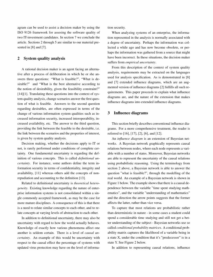
An influence diagram is an extension of Bayesian net-works. A Bayesian network graphically represents causalrelations between nodes, where each node represents a vari-able with a number of states. Moreover, Bayesian networksare able to represent the uncertainty of the causal relationsusing probabilistic reasoning. Using the terminology fromsection 2 above, a Bayesian network is able to answer thequestion ”what is feasible?”, through the modelling of thereal world. An example of a Bayesian network is shown inFigure 1 below. The example shows that there is a causal de-pendence between the variable ”time spent studying math-ematics”, and the variable ”understanding of mathematics”and the direction the arrow points suggests that the formeraffects the latter, rather than vice versa.

To capture that most relations are probabilistic ratherthan deterministic in nature - in some cases a student couldspend a considerable time studying and still not get a bet-ter understanding of the subject - Bayesian networks use socalled conditional probability matrices. A conditional prob-ability matrix captures the likelihood of a variable being ina state X, under the condition that it’s ”predecessor” is in astate Y. See Figure 2 below.

In addition to representing causal relations, influence

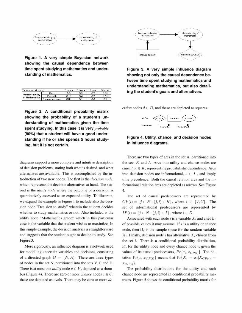
Figure 1. A very simple Bayesian networkshowing the causal dependence betweentime spent studying mathematics and under-standing of mathematics.

Figure 2. A conditional probability matrixshowing the probability of a student’s un-derstanding of mathematics given the timespent studying. In this case it is very probable(80%) that a student will have a good under-standing if he or she spends 5 hours study-ing, but it is not certain.

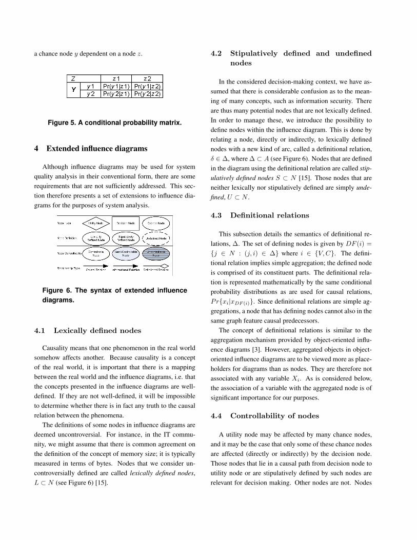
diagrams support a more complete and intuitive descriptionof decision problems, stating both what is desired, and whatalternatives are available. This is accomplished by the in-troduction of two new nodes. The first is the decision node,which represents the decision alternatives at hand. The sec-ond is the utility node where the outcome of a decision isquantitatively assessed as an expected utility. To illustrate,we expand the example in Figure 1 to include also the deci-sion node ”Decision to study” wherein the student decideswhether to study mathematics or not. Also included is theutility node ”Mathematics grade” which in this particularcase is the variable that the student wishes to maximize. Inthis simple example, the decision analysis is straightforwardand suggests that the student ought to decide to study. SeeFigure 3.

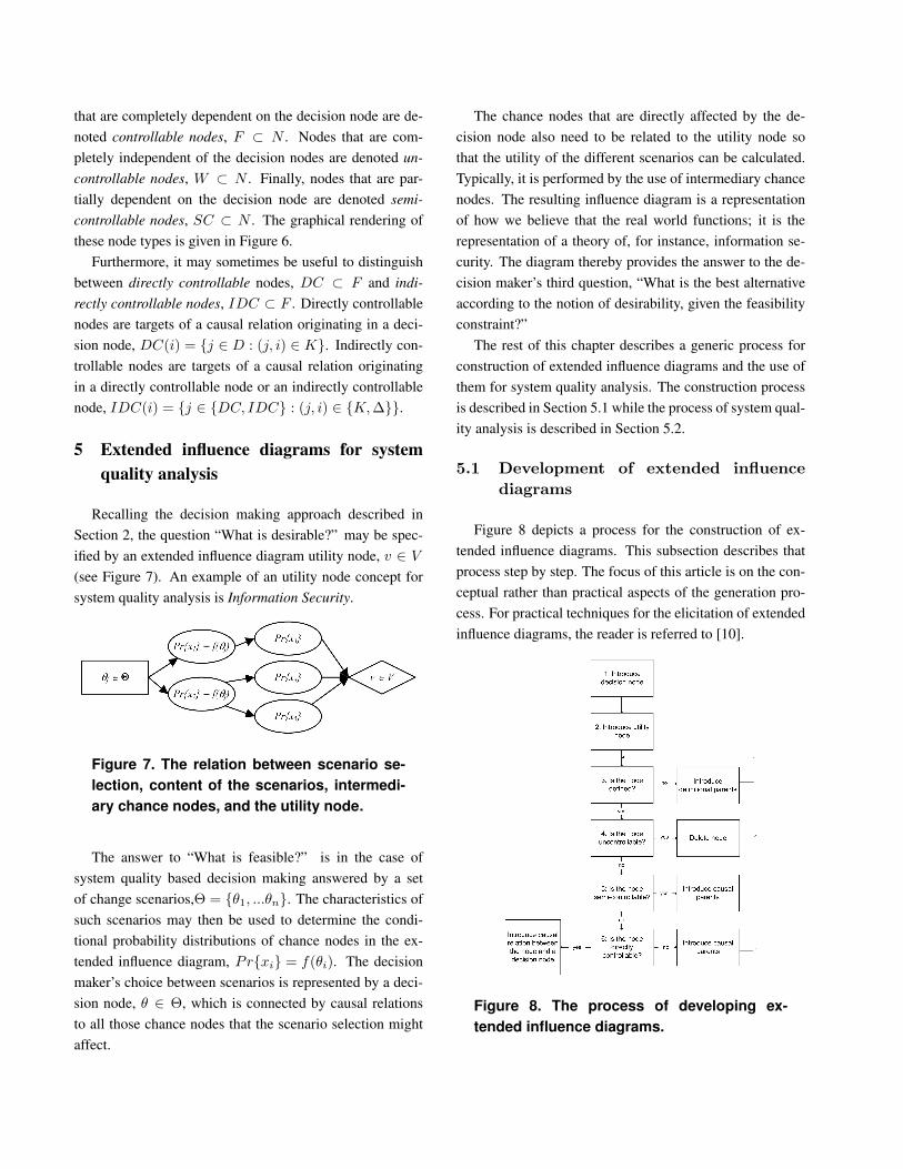
More rigorously, an influence diagram is a network usedfor modelling uncertain variables and decisions, consistingof a directed graph G = (N,A). There are three typesof nodes in the set N, partitioned into the sets V, C and D.There is at most one utility node v ∈ V , depicted as a rhom-bus (Figure 4). There are zero or more chance nodes c ∈ C,these are depicted as ovals. There may be zero or more de-

Figure 3. A very simple influence diagramshowing not only the causal dependence be-tween time spent studying mathematics andunderstanding mathematics, but also detail-ing the student’s goals and alternatives.

cision nodes d ∈ D, and these are depicted as squares.

Figure 4. Utility, chance, and decision nodesin influence diagrams.

There are two types of arcs in the set A, partitioned intothe sets K and I . Arcs into utility and chance nodes arecausal, κ ∈ K, representing probabilistic dependence. Arcsinto decision nodes are informational, ι ∈ I , and implytime precedence. Both the causal relation arcs and the in-formational relation arcs are depicted as arrows. See Figure4.

The set of causal predecessors are represented byCP (i) = j ∈ N : (j, i) ∈ K, where i ∈ V,C. Theset of informational predecessors are represented byIP (i) = j ∈ N : (j, i) ∈ I , where i ∈ D.

Associated with each node i is a variable Xi and a set Ωi

of possible values it may assume. If i is a utility or chancenode, then Ωi is the sample space for the random variableXi. Finally, decision node i has alternative Xi chosen fromthe set i. There is a conditional probability distribution,Pr, for the utility node and every chance node i, given thevalues of its causal predecessors, Prxi|xCP (i). The no-tation Prxi|xCP (i) means that PrXi = xi|XCP (i) =xCP (i).

The probability distributions for the utility and eachchance node are represented in conditional probability ma-trices. Figure 5 shows the conditional probability matrix for

a chance node y dependent on a node z.

Figure 5. A conditional probability matrix.

4 Extended influence diagrams

Although influence diagrams may be used for systemquality analysis in their conventional form, there are somerequirements that are not sufficiently addressed. This sec-tion therefore presents a set of extensions to influence dia-grams for the purposes of system analysis.

Figure 6. The syntax of extended influencediagrams.

4.1 Lexically defined nodes

Causality means that one phenomenon in the real worldsomehow affects another. Because causality is a conceptof the real world, it is important that there is a mappingbetween the real world and the influence diagrams, i.e. thatthe concepts presented in the influence diagrams are well-defined. If they are not well-defined, it will be impossibleto determine whether there is in fact any truth to the causalrelation between the phenomena.

The definitions of some nodes in influence diagrams aredeemed uncontroversial. For instance, in the IT commu-nity, we might assume that there is common agreement onthe definition of the concept of memory size; it is typicallymeasured in terms of bytes. Nodes that we consider un-controversially defined are called lexically defined nodes,L ⊂ N (see Figure 6) [15].

4.2 Stipulatively defined and undefinednodes

In the considered decision-making context, we have as-sumed that there is considerable confusion as to the mean-ing of many concepts, such as information security. Thereare thus many potential nodes that are not lexically defined.In order to manage these, we introduce the possibility todefine nodes within the influence diagram. This is done byrelating a node, directly or indirectly, to lexically definednodes with a new kind of arc, called a definitional relation,δ ∈ ∆, where ∆ ⊂ A (see Figure 6). Nodes that are definedin the diagram using the definitional relation are called stip-ulatively defined nodes S ⊂ N [15]. Those nodes that areneither lexically nor stipulatively defined are simply unde-fined, U ⊂ N .

4.3 Definitional relations

This subsection details the semantics of definitional re-lations, ∆. The set of defining nodes is given by DF (i) =j ∈ N : (j, i) ∈ ∆ where i ∈ V,C. The defini-tional relation implies simple aggregation; the defined nodeis comprised of its constituent parts. The definitional rela-tion is represented mathematically by the same conditionalprobability distributions as are used for causal relations,Prxi|xDF (i). Since definitional relations are simple ag-gregations, a node that has defining nodes cannot also in thesame graph feature causal predecessors.

The concept of definitional relations is similar to theaggregation mechanism provided by object-oriented influ-ence diagrams [3]. However, aggregated objects in object-oriented influence diagrams are to be viewed more as place-holders for diagrams than as nodes. They are therefore notassociated with any variable Xi. As is considered below,the association of a variable with the aggregated node is ofsignificant importance for our purposes.

4.4 Controllability of nodes

A utility node may be affected by many chance nodes,and it may be the case that only some of these chance nodesare affected (directly or indirectly) by the decision node.Those nodes that lie in a causal path from decision node toutility node or are stipulatively defined by such nodes arerelevant for decision making. Other nodes are not. Nodes

that are completely dependent on the decision node are de-noted controllable nodes, F ⊂ N . Nodes that are com-pletely independent of the decision nodes are denoted un-controllable nodes, W ⊂ N . Finally, nodes that are par-tially dependent on the decision node are denoted semi-controllable nodes, SC ⊂ N . The graphical rendering ofthese node types is given in Figure 6.

Furthermore, it may sometimes be useful to distinguishbetween directly controllable nodes, DC ⊂ F and indi-rectly controllable nodes, IDC ⊂ F . Directly controllablenodes are targets of a causal relation originating in a deci-sion node, DC(i) = j ∈ D : (j, i) ∈ K. Indirectly con-trollable nodes are targets of a causal relation originatingin a directly controllable node or an indirectly controllablenode, IDC(i) = j ∈ DC, IDC : (j, i) ∈ K, ∆.

5 Extended influence diagrams for systemquality analysis

Recalling the decision making approach described inSection 2, the question “What is desirable?” may be spec-ified by an extended influence diagram utility node, v ∈ V

(see Figure 7). An example of an utility node concept forsystem quality analysis is Information Security.

Figure 7. The relation between scenario se-lection, content of the scenarios, intermedi-ary chance nodes, and the utility node.

The answer to “What is feasible?” is in the case ofsystem quality based decision making answered by a setof change scenarios,Θ = θ1, ...θn. The characteristics ofsuch scenarios may then be used to determine the condi-tional probability distributions of chance nodes in the ex-tended influence diagram, Prxi = f(θi). The decisionmaker’s choice between scenarios is represented by a deci-sion node, θ ∈ Θ, which is connected by causal relationsto all those chance nodes that the scenario selection mightaffect.

The chance nodes that are directly affected by the de-cision node also need to be related to the utility node sothat the utility of the different scenarios can be calculated.Typically, it is performed by the use of intermediary chancenodes. The resulting influence diagram is a representationof how we believe that the real world functions; it is therepresentation of a theory of, for instance, information se-curity. The diagram thereby provides the answer to the de-cision maker’s third question, “What is the best alternativeaccording to the notion of desirability, given the feasibilityconstraint?”

The rest of this chapter describes a generic process forconstruction of extended influence diagrams and the use ofthem for system quality analysis. The construction processis described in Section 5.1 while the process of system qual-ity analysis is described in Section 5.2.

5.1 Development of extended influencediagrams

Figure 8 depicts a process for the construction of ex-tended influence diagrams. This subsection describes thatprocess step by step. The focus of this article is on the con-ceptual rather than practical aspects of the generation pro-cess. For practical techniques for the elicitation of extendedinfluence diagrams, the reader is referred to [10].

Figure 8. The process of developing ex-tended influence diagrams.

5.1.1 Step one: Introduce decision node

At the very start, the decision node should be identified.As mentioned above decision nodes represent the choicebetween different change scenarios, such as the choice be-tween integrating a set of systems, replacing them, or main-taining the status quo.

5.1.2 Step two: Introduce utility node

The second step is to define the utility node. The util-ity node is the target of the system quality analysis. Ex-amples of utility nodes are information security, modifi-ability, performance and reliability. When defining theutility node, its variable type should also be decidedon, e.g. Low,Medium,High, Present,Absent,True, False, or 0, 1, 2, 3, 4.

5.1.3 Step three: Is the node defined?

The third step is to determine whether the node is lexicallydefined, stipulatively defined or undefined. Recall that anode is lexically defined if we can assume that there is com-mon agreement on its definition. Although almost all defini-tions can be challenged, concepts that would normally qual-ify as lexically defined include weight in kilograms, num-ber of processors or number of users. For many concepts,however, such as information security, architecture qualityand competence there is no universal definition even by verypragmatic standards.

If the node is not lexically defined, it needs to be stipu-latively defined. This is accomplished with the definitionalrelationship presented in the previous chapter. As an exam-ple, the node Availability might be defined by the two nodesMean Time To Failure and Mean Time To Repair. The stipu-lative definition of a node results in the introduction of newnodes into the diagram. When new nodes are introduced,this affects the conditional probability matrices of the childnodes. These must therefore also be specified, thereby de-tailing the dependencies between the parents and the child.When an undefined node has been stipulatively defined, thediagram construction process refocuses on one of the newnodes and returns to the third step.

5.1.4 Step four: Is the node uncontrollable?

For each defined node, the fourth step considers whether thenode is uncontrollable. Recall that uncontrollable nodes areunaffected by variable changes in the decision node; thismeans that potential variations in the value of the uncon-trollable node are unrelated to the choices of the decisionmaker. If the node is uncontrollable, it will not provide deci-sion supporting information, so there is no need to continueexploring this branch of the diagram. The node is thereforedeleted, the process refocuses on the next unexamined nodeand returns to the third step.

5.1.5 Step five: Is the node semi-controllable?

Step five queries whether the node under consideration issemi-controllable. Semi-controllable nodes are affectedboth by the decision makers choices and other, uncontrol-lable, phenomena. If a node is semi-controllable, it isimportant to separate those aspects which are controllablefrom those which are not. Therefore, new nodes are intro-duced into the diagram with causal relations to the semi-controllable node under consideration. As an example, wemight believe that the semi-controllable node Mean TimeTo Repair is causally affected by both the Maintainabilityof the system and Flexibility of Working Hour Regulations.Of these, the maintainability might be controllable, whilethe working hour regulations might be beyond the decisionmakers domain of control. In the same manner as in thesecond step, the involved conditional probability matricesneed to be specified. The diagram construction process onceagain refocuses on one of the new nodes and returns to thethird step.

5.1.6 Step six: Is the node directly controllable?

In the sixth step, the process considers whether the nodesare directly or indirectly controllable. A directly control-lable phenomenon is an immediate consequence of the de-cision makers choice. For instance, if a scenario is chosenwhere one system is replaced by another, this may directlyentail that the CPU speed is increased. Directly control-lable nodes are causally connected to the decision node. Fornodes that do not seem to be directly controllable, one orseveral new nodes are introduced into the diagram, the fo-cus shifts to the first of these, and the process returns to thethird step.

When the whole process is finished, the result is an ex-tended influence diagram where the nodes are causally af-fected by the decision node and in turn either causally affectthe utility node, or do so by definition. No nodes are unde-fined, and uncontrollable nodes have no parents.

5.2 Analyzing with extended influencediagrams

When an extended influence diagram has been con-structed, it may be used to compare and assess the qualityof different system scenarios.

5.2.1 Linking scenarios to extended influence dia-grams

In extended influence diagrams, decision nodes representa choice between alternatives. In system quality analysis,these alternatives are concretized by different change sce-narios. We will now consider how the information repre-sented in the scenarios is introduced into the extended in-fluence diagrams.

A change scenario, say Scenario X, can contain a set ofentities. Considering one of these entities, say the SystemA entity, we find that it features a set of attributes, Mem-ory Size, Lines Of Code, etc. The value of each of theseattributes is represented in a conditional probability matrix,PrMemorySizeEA = msi. This approach retains thepossibility to present attribute values deterministically byallowing only zero or unity probabilities in the matrix.

The directly controllable nodes in a extended influencediagram, i.e. the chance nodes that are directly linked to thedecision node, consitute the coupling to the scenario. Ex-amining one of these nodes in detail, we find that it might benamed Memory Size. The link between the scenario and theextended influence diagram is concretely specified by thefollowing requirement: the Memory Size node’s probabilitygiven that Scenario X is selected is equal to the conditionalprobability of the Memory Size attribute of the System Aentity, i.e. PrMemorySizeEID = msi|dScenarioX =PrMemorySizeEA = msi.

5.2.2 Calculating the results

The conditional probability distributions of the directly con-trollable nodes are thus retrieved from the change scenar-ios. The higher-level conditional probability matrices were

determined already during the extended influence diagramconstruction process. The value of the utility node cantherefore be calculated employing standard methods [6][12]. There are several tools available on the market forthese calculations, such as Genie [9] and Hugin [3].

6 The ISO/IEC 9126 extended influence dia-gram

This section provides an exemple of the construction ofextended influence diagrams and the use of them for systemquality analysis. The former is described in Section 6.1 andaims at demonstrating not only the development process initself, but also the expressive possibilities of the extendedinfluence diagram language. The perspective of the diagramuser is described in Section 6.2, where the developed ex-tended influence diagram is used by a decision maker. Thecontext is an IT-investment situation where an IT-decisionmaker must choose between one of two possible scenarios.The example relates to system qualities and to the ISO/IEC9126 standard [4][5].

6.1 Development of extended influencediagrams

A process for the development of extended influence dia-grams described in the previous section and in Figure 8 isfollowed in the presented example.

The example decision situation is a company that needsto procure a new Customer Relations Management (CRM)system. The Chief Information Officer (CIO) is responsi-ble for making the decision which system to buy, and isgiven the choice between scenario 1, the decision makerpurchases system A, and Scenario 2, the decision makerpurchases system B. System A is an extension of the En-terprise Resource Planning (ERP) system already imple-mented at the company, and system B is a best-of-breedsolution. Life Cycle Cost analyses indicate that the costs as-sociated with choosing either one of the scenarios are closeto identical, so the only parameter that separates the scenar-ios is their respective software quality; the scenario with thehighest quality will be chosen in the end. Software qual-ity refers to the functional and non-functional properties ofa software system, e.g. usability, efficiency etc. To deter-mine which of the two systems has the highest quality the

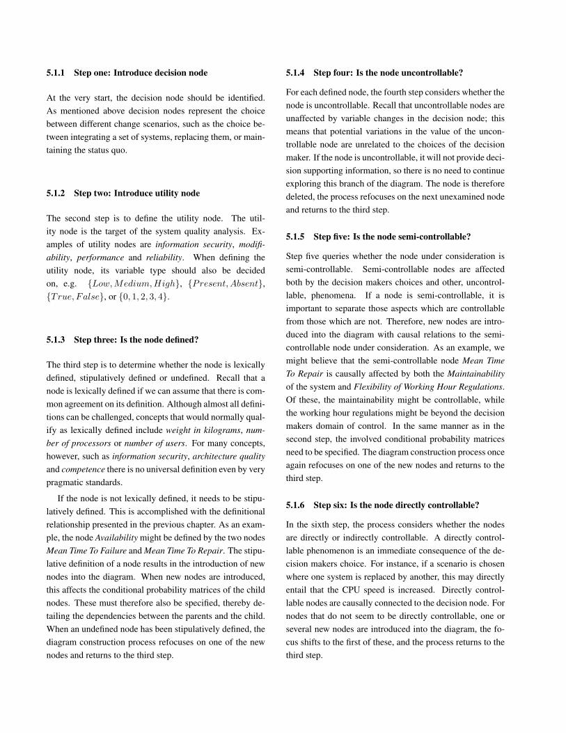
CIO orders his IT-staff to conduct measurements of existingimplementations of systems A and B. Using extended influ-ence diagrams for the analysis, ”Quality” is chosen as theutility node.

Figure 9. The utility and decision nodes.

Following the flowchart of Figure 8, we see that the util-ity node is not defined, neither lexically nor stipulatively.Thus, we need to define it using definitional parents in theform of chance nodes. In ISO/IEC 9126 [4] we find that thequality of a software system is defined by the functionality,reliability, usability, efficiency, maintainability, and porta-bility.

Figure 10. The utility node quality defined bythe nodes functionality, reliability, usability,efficiency, maintainability and portability.

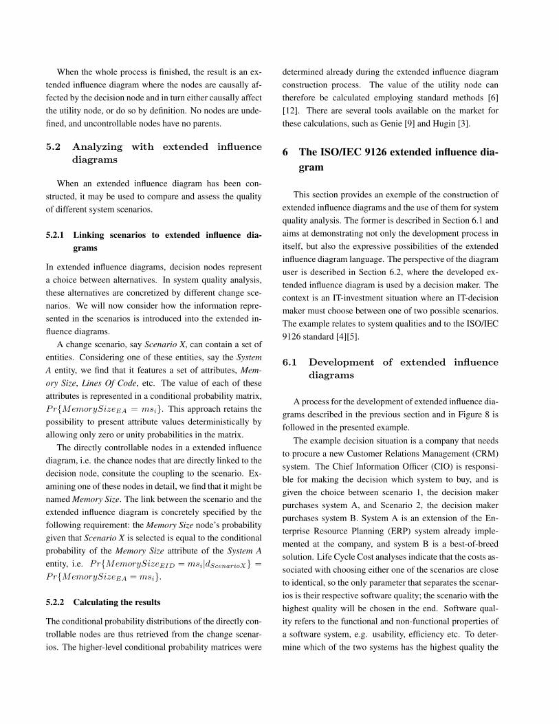
Restarting at the top of the flowchart for the new nodes,none of these concepts are considered to be lexically de-fined. Fortunately however, these concepts have all beenstipulatively defined in the ISO/IEC 9126 standard [4]. E.g.Maintainability is defined by the concepts Analysability,Changeability, Stability, Testability. In Figure 11 all nodeshave been stipulatively defined using the ISO standard.

Once again restarting at the top of the flow chart, wefind that these new nodes are not considered to be lexicallydefined. Since we are using ISO 9126 for measuring al-ready existing systems, it is the external metrics describedin ISO 9126-2 [5] which will be used. ISO 9126-2 has stip-ulatively defined all nodes currently in the extended influ-ence diagram, e.g. changeability is measured in terms ofthe five metrics change cycle efficiency, change implemen-tation elapse time, modification complexity, parameterisedmodifiability, and software change control capability.

Having a look at the flow chart we find that thesenodes are defined, they are not uncontrollable, not semi-

Figure 11. The nodes functionality, reliabil-ity, usability, efficiency, maintainability andportability defined using the 9126 ISO stan-dard.

Figure 12. The node changeability definedusing the 9126 ISO standard.

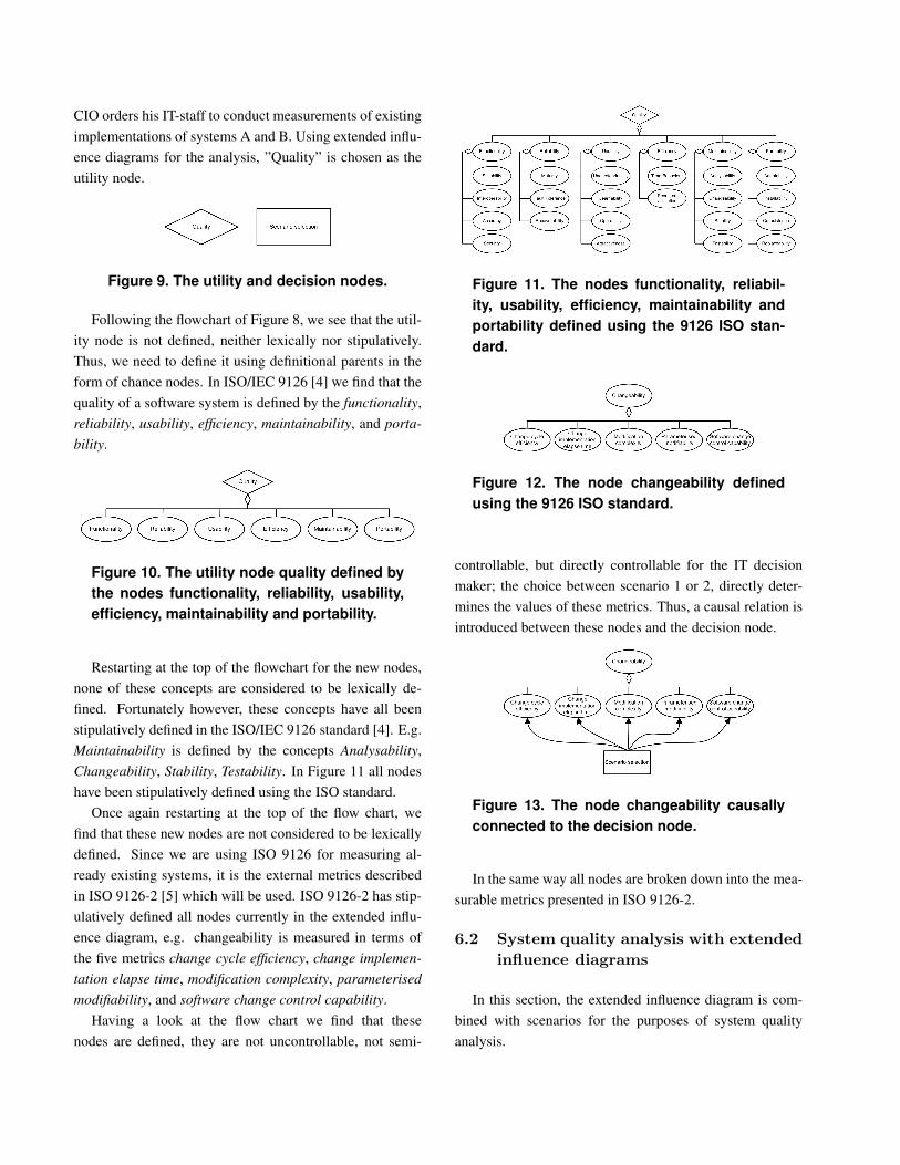
controllable, but directly controllable for the IT decisionmaker; the choice between scenario 1 or 2, directly deter-mines the values of these metrics. Thus, a causal relation isintroduced between these nodes and the decision node.

Figure 13. The node changeability causallyconnected to the decision node.

In the same way all nodes are broken down into the mea-surable metrics presented in ISO 9126-2.

6.2 System quality analysis with extendedinfluence diagrams

In this section, the extended influence diagram is com-bined with scenarios for the purposes of system qualityanalysis.

Recall the decision situation presented earlier in this sec-tion, the choice between Scenario 1 purchasing System A orScenario 2 purchasing System B. Using the extended influ-ence diagram based on ISO/IEC 9126 gives the CIO valu-able support as to which system to choose. All nodes con-nected to the decion node in the diagram are defined anddirectly controllable for the decision maker, the next stepis to collect the values for these nodes. How to collect thevalues for these nodes is described in the standard, e.g. thenode change cycle efficiency is measured by monitoring theinteraction between user and supplier and by recording thetime taken from the initial user’s request to the resolution ofproblem.

6.2.1 Conditional probability distributions of directlycontrollable nodes

Each node is associated with a conditional probability dis-tribution, these distributions contain the values of the di-rectly controllable nodes. Below we present the conditionalprobability distributions for the directly controllable nodesdefining changeability. In this case, as in many others, thecollected measuraments are not completely certain. As isshown in Figure 14 below, the choice of scenario 1 (i.e. tobuy system A) will probably lead to a high level of softwarechange control capability. The majority of measurementsindicate this, but not all which means that there is some un-certainty regarding what the outcome will be (20 % uncer-tainty in this case).

Figure 14. Conditional probability matrices ofthe directly controllable chance nodes.

6.2.2 Calculating the results

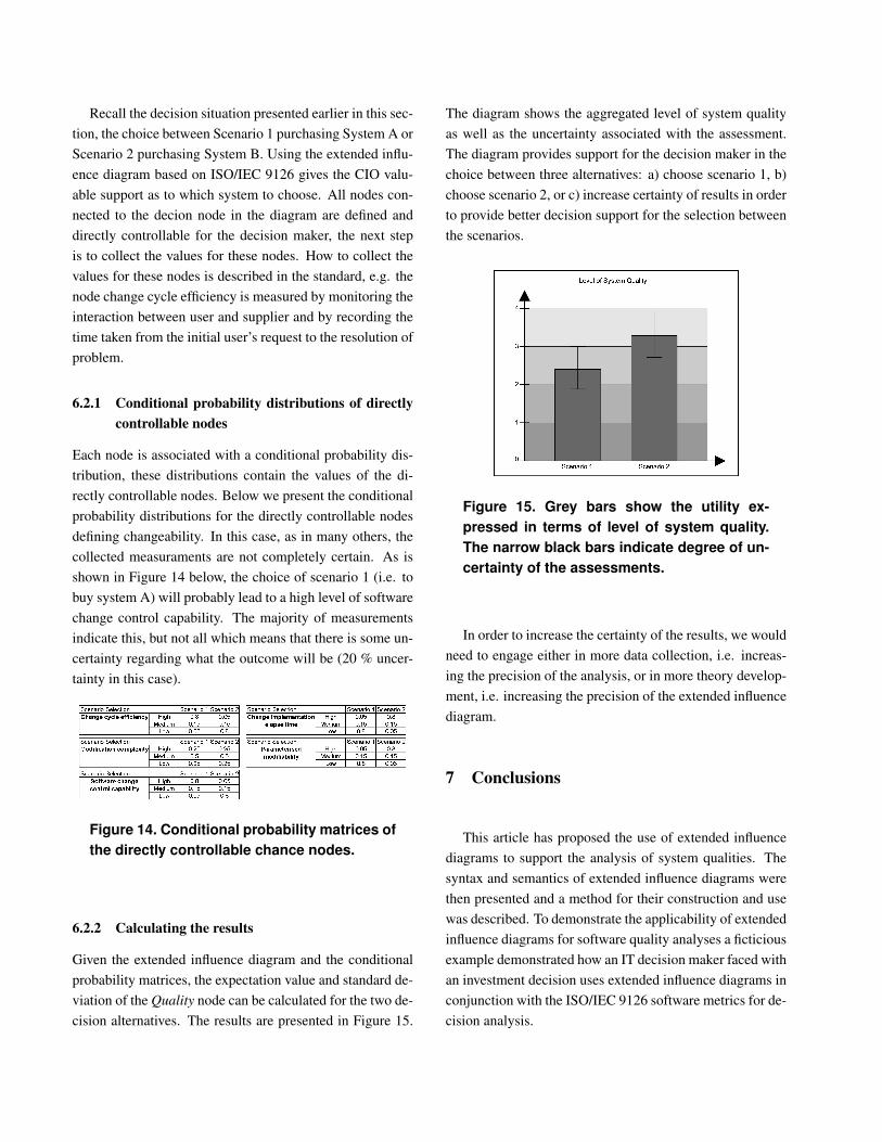
Given the extended influence diagram and the conditionalprobability matrices, the expectation value and standard de-viation of the Quality node can be calculated for the two de-cision alternatives. The results are presented in Figure 15.

The diagram shows the aggregated level of system qualityas well as the uncertainty associated with the assessment.The diagram provides support for the decision maker in thechoice between three alternatives: a) choose scenario 1, b)choose scenario 2, or c) increase certainty of results in orderto provide better decision support for the selection betweenthe scenarios.

Figure 15. Grey bars show the utility ex-pressed in terms of level of system quality.The narrow black bars indicate degree of un-certainty of the assessments.

In order to increase the certainty of the results, we wouldneed to engage either in more data collection, i.e. increas-ing the precision of the analysis, or in more theory develop-ment, i.e. increasing the precision of the extended influencediagram.

7 Conclusions

This article has proposed the use of extended influencediagrams to support the analysis of system qualities. Thesyntax and semantics of extended influence diagrams werethen presented and a method for their construction and usewas described. To demonstrate the applicability of extendedinfluence diagrams for software quality analyses a ficticiousexample demonstrated how an IT decision maker faced withan investment decision uses extended influence diagrams inconjunction with the ISO/IEC 9126 software metrics for de-cision analysis.

References

[1] R. A. Howard. Decision analysis: Practice and promise.Management Science, 34(6), 1988.

[2] R. A. Howard and J. E. Matheson. Influence diagrams. De-cision Analysis, 2(3), 1983.

[3] Hugin Expert A/S. HUGIN API Reference Manual, Version6.3, 2004.

[4] International Organization for Standardization. ISO/IEC TR9126-1 Technical Report - Software Engineering - ProductQuality - Part 1: Quality model, 2001.

[5] International Organization for Standardization. ISO/IEC TR9126-2 Technical Report - Software Engineering - ProductQuality - Part 2: External Metrics, 2003.

[6] F. V. Jensen. Bayesian Networks and Decision Graphs.Springer, 2001.

[7] P. Johnson, R. Lagerstrom, P. Narman, and M. Simonsson.Enterprise architecture analysis with extended influence dia-grams. To appear in Information System Frontiers, 2006.

[8] P. Johnson, R. Lagerstrom, P. Narman, and M. Simons-son. Extended influence diagrams for enterprise architectureanalysis. In Proceedings of the Tenth IEEE InternationalEDOC Conference (EDOC 2006), 2006.

[9] D. S. Laboratory. Genie On-Line Help, 2006.[10] R. Lagerstrom, P. Johnson, and P. Narman. Extended in-

fluence diagram generation for interoperability analysis. Toappear, 2007.

[11] P. Liu, P. Ammann, and S. Jajodia. Rewriting histories: Re-covering from malicious transactions. Distributed and Par-alell Databases, 8, 2000.

[12] R. Neapolitan. Learning Bayesian Networks. Pearson Edu-cation, 2004.

[13] S. Poslad and M. Calisti. Towards improved trust and se-curity in fipa agent platforms. In Autonomous Agents 2000Workshop on Deception, Fraud and Trust in Agent Societies,2000.

[14] A. Rubenstein. Modeling Bounded Rationality. The MITPress, 1998.

[15] M. Scriven. Definitions in analytical philosophy. Philosoph-ical Studies, 5(3), 1954.

[16] R. Shachter. Evaluating influence diagrams. Operations Re-search, 34(6), 1986.

[17] R. Shachter. Probabilistic inference and influence diagrams.Operations Research, 36(4), 1988.