Embed Size (px)
Citation preview

Introduction to Spatial Econometrics
© 2009 by Taylor & Francis Group, LLC
STATISTICS: Textbooks and MonographsD. B. Owen
Founding Editor, 1972–1991
Editors
N. BalakrishnanMcMaster University
William R. SchucanySouthern Methodist University
Editorial Board
Thomas B. BarkerRochester Institute of Technology
Paul R. GarveyThe MITRE Corporation
Subir GhoshUniversity of California, Riverside
David E. A. GilesUniversity of Victoria
Arjun K. GuptaBowling Green State
University
Nicholas JewellUniversity of California, Berkeley
Sastry G. PantulaNorth Carolina State
University
Daryl S. PaulsonBiosciences Laboratories, Inc.
Aman UllahUniversity of California,
Riverside
Brian E. WhiteThe MITRE Corporation
© 2009 by Taylor & Francis Group, LLC
STATISTICS: Textbooks and Monographs
Recent Titles
Visualizing Statistical Models and Concepts, R. W. Farebrother and Michaël Schyns
Financial and Actuarial Statistics: An Introduction, Dale S. Borowiak
Nonparametric Statistical Inference, Fourth Edition, Revised and Expanded, Jean Dickinson Gibbons and Subhabrata Chakraborti
Computer-Aided Econometrics, edited by David E.A. Giles
The EM Algorithm and Related Statistical Models, edited by Michiko Watanabe and Kazunori Yamaguchi
Multivariate Statistical Analysis, Second Edition, Revised and Expanded, Narayan C. Giri
Computational Methods in Statistics and Econometrics, Hisashi Tanizaki
Applied Sequential Methodologies: Real-World Examples with Data Analysis, edited by Nitis Mukhopadhyay, Sujay Datta, and Saibal Chattopadhyay
Handbook of Beta Distribution and Its Applications, edited by Arjun K. Gupta and Saralees Nadarajah
Item Response Theory: Parameter Estimation Techniques, Second Edition, edited by Frank B. Baker and Seock-Ho Kim
Statistical Methods in Computer Security, edited by William W. S. Chen
Elementary Statistical Quality Control, Second Edition, John T. Burr
Data Analysis of Asymmetric Structures, Takayuki Saito and Hiroshi Yadohisa
Mathematical Statistics with Applications, Asha Seth Kapadia, Wenyaw Chan, and Lemuel Moyé
Advances on Models, Characterizations and Applications, N. Balakrishnan, I. G. Bairamov, and O. L. Gebizlioglu
Survey Sampling: Theory and Methods, Second Edition, Arijit Chaudhuri and Horst Stenger
Statistical Design of Experiments with Engineering Applications, Kamel Rekab and Muzaffar Shaikh
Quality by Experimental Design, Third Edition, Thomas B. Barker
Handbook of Parallel Computing and Statistics, Erricos John Kontoghiorghes
Statistical Inference Based on Divergence Measures, Leandro Pardo
A Kalman Filter Primer, Randy Eubank
Introductory Statistical Inference, Nitis Mukhopadhyay
Handbook of Statistical Distributions with Applications, K. Krishnamoorthy
A Course on Queueing Models, Joti Lal Jain, Sri Gopal Mohanty, and Walter Böhm
Univariate and Multivariate General Linear Models: Theory and Applications with SAS, Second Edition, Kevin Kim and Neil Timm
Randomization Tests, Fourth Edition, Eugene S. Edgington and Patrick Onghena
Design and Analysis of Experiments: Classical and Regression Approaches with SAS, Leonard C. Onyiah
Analytical Methods for Risk Management: A Systems Engineering Perspective, Paul R. Garvey
Confidence Intervals in Generalized Regression Models, Esa Uusipaikka
Introduction to Spatial Econometrics, James LeSage and R. Kelley Pace
© 2009 by Taylor & Francis Group, LLC

Introduction to Spatial Econometrics
James LeSageTexas State University-San Marcos
San Marcos, Texas, U.S.A.
R. Kelley PaceLouisiana State University
Baton Rouge, Louisiana, U.S.A.
© 2009 by Taylor & Francis Group, LLC

Chapman & Hall/CRCTaylor & Francis Group6000 Broken Sound Parkway NW, Suite 300Boca Raton, FL 33487‑2742
© 2009 by Taylor & Francis Group, LLC Chapman & Hall/CRC is an imprint of Taylor & Francis Group, an Informa business
No claim to original U.S. Government worksPrinted in the United States of America on acid‑free paper10 9 8 7 6 5 4 3 2 1
International Standard Book Number‑13: 978‑1‑4200‑6424‑7 (Hardcover)
This book contains information obtained from authentic and highly regarded sources. Reasonable efforts have been made to publish reliable data and information, but the author and publisher can‑not assume responsibility for the validity of all materials or the consequences of their use. The authors and publishers have attempted to trace the copyright holders of all material reproduced in this publication and apologize to copyright holders if permission to publish in this form has not been obtained. If any copyright material has not been acknowledged please write and let us know so we may rectify in any future reprint.
Except as permitted under U.S. Copyright Law, no part of this book may be reprinted, reproduced, transmitted, or utilized in any form by any electronic, mechanical, or other means, now known or hereafter invented, including photocopying, microfilming, and recording, or in any information storage or retrieval system, without written permission from the publishers.
For permission to photocopy or use material electronically from this work, please access www.copy‑right.com (http://www.copyright.com/) or contact the Copyright Clearance Center, Inc. (CCC), 222 Rosewood Drive, Danvers, MA 01923, 978‑750‑8400. CCC is a not‑for‑profit organization that pro‑vides licenses and registration for a variety of users. For organizations that have been granted a photocopy license by the CCC, a separate system of payment has been arranged.
Trademark Notice: Product or corporate names may be trademarks or registered trademarks, and are used only for identification and explanation without intent to infringe.
Library of Congress Cataloging‑in‑Publication Data
LeSage, James P.Introduction to spatial econometrics / James LeSage, Robert Kelley Pace.
p. cm. ‑‑ (Statistics : a series of textbooks and monographs ; 196)Includes bibliographical references and index.ISBN‑13: 978‑1‑4200‑6424‑7 (alk. paper)ISBN‑10: 1‑4200‑6424‑X (alk. paper)1. Space in economics‑‑Econometric models. 2. Space in
economics‑‑Mathematical models. I. Pace, Robert Kelley. II. Title. III. Series.
HT388.L47 2009330.01’5195‑‑dc22 2008038890
Visit the Taylor & Francis Web site athttp://www.taylorandfrancis.com
and the CRC Press Web site athttp://www.crcpress.com
© 2009 by Taylor & Francis Group, LLC
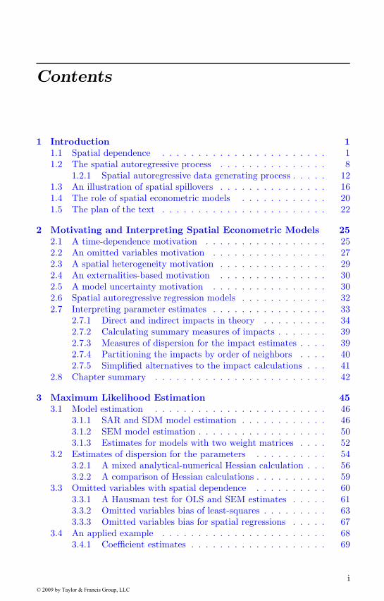
Contents
1 Introduction 11.1 Spatial dependence . . . . . . . . . . . . . . . . . . . . . . . 11.2 The spatial autoregressive process . . . . . . . . . . . . . . . 8
1.2.1 Spatial autoregressive data generating process . . . . . 121.3 An illustration of spatial spillovers . . . . . . . . . . . . . . . 161.4 The role of spatial econometric models . . . . . . . . . . . . 201.5 The plan of the text . . . . . . . . . . . . . . . . . . . . . . . 22
2 Motivating and Interpreting Spatial Econometric Models 252.1 A time-dependence motivation . . . . . . . . . . . . . . . . . 252.2 An omitted variables motivation . . . . . . . . . . . . . . . . 272.3 A spatial heterogeneity motivation . . . . . . . . . . . . . . . 292.4 An externalities-based motivation . . . . . . . . . . . . . . . 302.5 A model uncertainty motivation . . . . . . . . . . . . . . . . 302.6 Spatial autoregressive regression models . . . . . . . . . . . . 322.7 Interpreting parameter estimates . . . . . . . . . . . . . . . . 33
2.7.1 Direct and indirect impacts in theory . . . . . . . . . 342.7.2 Calculating summary measures of impacts . . . . . . . 392.7.3 Measures of dispersion for the impact estimates . . . . 392.7.4 Partitioning the impacts by order of neighbors . . . . 402.7.5 Simplified alternatives to the impact calculations . . . 41
2.8 Chapter summary . . . . . . . . . . . . . . . . . . . . . . . . 42
3 Maximum Likelihood Estimation 453.1 Model estimation . . . . . . . . . . . . . . . . . . . . . . . . 46
3.1.1 SAR and SDM model estimation . . . . . . . . . . . . 463.1.2 SEM model estimation . . . . . . . . . . . . . . . . . . 503.1.3 Estimates for models with two weight matrices . . . . 52
3.2 Estimates of dispersion for the parameters . . . . . . . . . . 543.2.1 A mixed analytical-numerical Hessian calculation . . . 563.2.2 A comparison of Hessian calculations . . . . . . . . . . 59
3.3 Omitted variables with spatial dependence . . . . . . . . . . 603.3.1 A Hausman test for OLS and SEM estimates . . . . . 613.3.2 Omitted variables bias of least-squares . . . . . . . . . 633.3.3 Omitted variables bias for spatial regressions . . . . . 67
3.4 An applied example . . . . . . . . . . . . . . . . . . . . . . . 683.4.1 Coefficient estimates . . . . . . . . . . . . . . . . . . . 69
i© 2009 by Taylor & Francis Group, LLC
ii
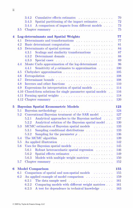
3.4.2 Cumulative effects estimates . . . . . . . . . . . . . . 703.4.3 Spatial partitioning of the impact estimates . . . . . . 723.4.4 A comparison of impacts from different models . . . . 73
3.5 Chapter summary . . . . . . . . . . . . . . . . . . . . . . . . 75
4 Log-determinants and Spatial Weights 774.1 Determinants and transformations . . . . . . . . . . . . . . . 774.2 Basic determinant computation . . . . . . . . . . . . . . . . 814.3 Determinants of spatial systems . . . . . . . . . . . . . . . . 84
4.3.1 Scalings and similarity transformations . . . . . . . . 874.3.2 Determinant domain . . . . . . . . . . . . . . . . . . . 884.3.3 Special cases . . . . . . . . . . . . . . . . . . . . . . . 89
4.4 Monte Carlo approximation of the log-determinant . . . . . . 964.4.1 Sensitivity of ρ estimates to approximation . . . . . . 100
4.5 Chebyshev approximation . . . . . . . . . . . . . . . . . . . . 1054.6 Extrapolation . . . . . . . . . . . . . . . . . . . . . . . . . . 1084.7 Determinant bounds . . . . . . . . . . . . . . . . . . . . . . . 1084.8 Inverses and other functions . . . . . . . . . . . . . . . . . . 1104.9 Expressions for interpretation of spatial models . . . . . . . . 1144.10 Closed-form solutions for single parameter spatial models . . 1164.11 Forming spatial weights . . . . . . . . . . . . . . . . . . . . . 1184.12 Chapter summary . . . . . . . . . . . . . . . . . . . . . . . . 120
5 Bayesian Spatial Econometric Models 1235.1 Bayesian methodology . . . . . . . . . . . . . . . . . . . . . . 1245.2 Conventional Bayesian treatment of the SAR model . . . . . 127
5.2.1 Analytical approaches to the Bayesian method . . . . 1275.2.2 Analytical solution of the Bayesian spatial model . . . 130
5.3 MCMC estimation of Bayesian spatial models . . . . . . . . 1335.3.1 Sampling conditional distributions . . . . . . . . . . . 1335.3.2 Sampling for the parameter ρ . . . . . . . . . . . . . . 136
5.4 The MCMC algorithm . . . . . . . . . . . . . . . . . . . . . 1395.5 An applied illustration . . . . . . . . . . . . . . . . . . . . . 1425.6 Uses for Bayesian spatial models . . . . . . . . . . . . . . . . 145
5.6.1 Robust heteroscedastic spatial regression . . . . . . . 1465.6.2 Spatial effects estimates . . . . . . . . . . . . . . . . . 1495.6.3 Models with multiple weight matrices . . . . . . . . . 150
5.7 Chapter summary . . . . . . . . . . . . . . . . . . . . . . . . 152
6 Model Comparison 1556.1 Comparison of spatial and non-spatial models . . . . . . . . 1556.2 An applied example of model comparison . . . . . . . . . . . 159
6.2.1 The data sample used . . . . . . . . . . . . . . . . . . 1616.2.2 Comparing models with different weight matrices . . . 1616.2.3 A test for dependence in technical knowledge . . . . . 163
© 2009 by Taylor & Francis Group, LLC
iii
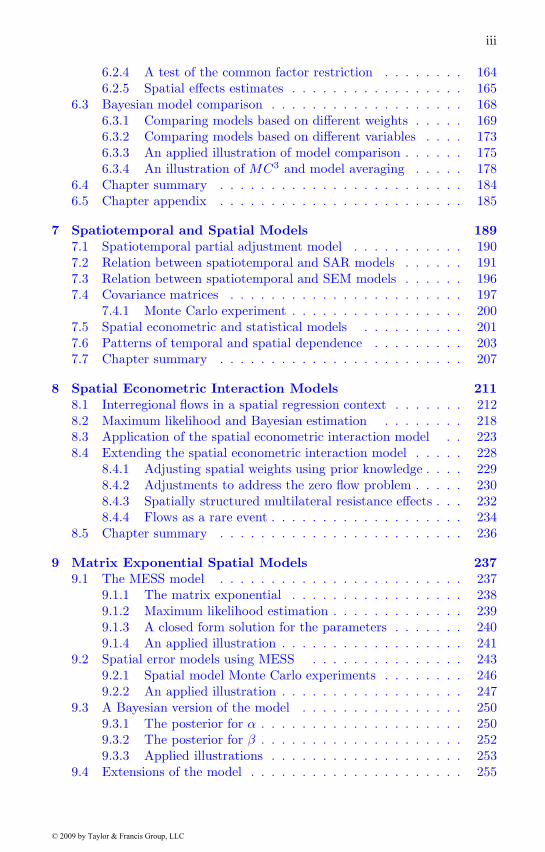
6.2.4 A test of the common factor restriction . . . . . . . . 1646.2.5 Spatial effects estimates . . . . . . . . . . . . . . . . . 165
6.3 Bayesian model comparison . . . . . . . . . . . . . . . . . . . 1686.3.1 Comparing models based on different weights . . . . . 1696.3.2 Comparing models based on different variables . . . . 1736.3.3 An applied illustration of model comparison . . . . . . 1756.3.4 An illustration of MC3 and model averaging . . . . . 178
6.4 Chapter summary . . . . . . . . . . . . . . . . . . . . . . . . 1846.5 Chapter appendix . . . . . . . . . . . . . . . . . . . . . . . . 185
7 Spatiotemporal and Spatial Models 1897.1 Spatiotemporal partial adjustment model . . . . . . . . . . . 1907.2 Relation between spatiotemporal and SAR models . . . . . . 1917.3 Relation between spatiotemporal and SEM models . . . . . . 1967.4 Covariance matrices . . . . . . . . . . . . . . . . . . . . . . . 197
7.4.1 Monte Carlo experiment . . . . . . . . . . . . . . . . . 2007.5 Spatial econometric and statistical models . . . . . . . . . . 2017.6 Patterns of temporal and spatial dependence . . . . . . . . . 2037.7 Chapter summary . . . . . . . . . . . . . . . . . . . . . . . . 207
8 Spatial Econometric Interaction Models 2118.1 Interregional flows in a spatial regression context . . . . . . . 2128.2 Maximum likelihood and Bayesian estimation . . . . . . . . 2188.3 Application of the spatial econometric interaction model . . 2238.4 Extending the spatial econometric interaction model . . . . . 228
8.4.1 Adjusting spatial weights using prior knowledge . . . . 2298.4.2 Adjustments to address the zero flow problem . . . . . 2308.4.3 Spatially structured multilateral resistance effects . . . 2328.4.4 Flows as a rare event . . . . . . . . . . . . . . . . . . . 234
8.5 Chapter summary . . . . . . . . . . . . . . . . . . . . . . . . 236
9 Matrix Exponential Spatial Models 2379.1 The MESS model . . . . . . . . . . . . . . . . . . . . . . . . 237
9.1.1 The matrix exponential . . . . . . . . . . . . . . . . . 2389.1.2 Maximum likelihood estimation . . . . . . . . . . . . . 2399.1.3 A closed form solution for the parameters . . . . . . . 2409.1.4 An applied illustration . . . . . . . . . . . . . . . . . . 241
9.2 Spatial error models using MESS . . . . . . . . . . . . . . . 2439.2.1 Spatial model Monte Carlo experiments . . . . . . . . 2469.2.2 An applied illustration . . . . . . . . . . . . . . . . . . 247
9.3 A Bayesian version of the model . . . . . . . . . . . . . . . . 2509.3.1 The posterior for α . . . . . . . . . . . . . . . . . . . . 2509.3.2 The posterior for β . . . . . . . . . . . . . . . . . . . . 2529.3.3 Applied illustrations . . . . . . . . . . . . . . . . . . . 253
9.4 Extensions of the model . . . . . . . . . . . . . . . . . . . . . 255
© 2009 by Taylor & Francis Group, LLC
iv
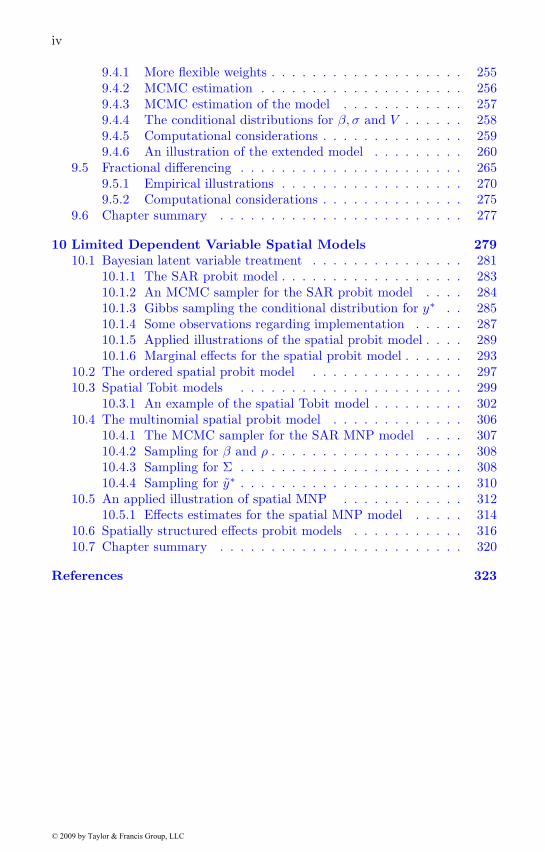
9.4.1 More flexible weights . . . . . . . . . . . . . . . . . . . 2559.4.2 MCMC estimation . . . . . . . . . . . . . . . . . . . . 2569.4.3 MCMC estimation of the model . . . . . . . . . . . . 2579.4.4 The conditional distributions for β, σ and V . . . . . . 2589.4.5 Computational considerations . . . . . . . . . . . . . . 2599.4.6 An illustration of the extended model . . . . . . . . . 260
9.5 Fractional differencing . . . . . . . . . . . . . . . . . . . . . . 2659.5.1 Empirical illustrations . . . . . . . . . . . . . . . . . . 2709.5.2 Computational considerations . . . . . . . . . . . . . . 275
9.6 Chapter summary . . . . . . . . . . . . . . . . . . . . . . . . 277
10 Limited Dependent Variable Spatial Models 27910.1 Bayesian latent variable treatment . . . . . . . . . . . . . . . 281
10.1.1 The SAR probit model . . . . . . . . . . . . . . . . . . 28310.1.2 An MCMC sampler for the SAR probit model . . . . 28410.1.3 Gibbs sampling the conditional distribution for y∗ . . 28510.1.4 Some observations regarding implementation . . . . . 28710.1.5 Applied illustrations of the spatial probit model . . . . 28910.1.6 Marginal effects for the spatial probit model . . . . . . 293
10.2 The ordered spatial probit model . . . . . . . . . . . . . . . 29710.3 Spatial Tobit models . . . . . . . . . . . . . . . . . . . . . . 299
10.3.1 An example of the spatial Tobit model . . . . . . . . . 30210.4 The multinomial spatial probit model . . . . . . . . . . . . . 306
10.4.1 The MCMC sampler for the SAR MNP model . . . . 30710.4.2 Sampling for β and ρ . . . . . . . . . . . . . . . . . . . 30810.4.3 Sampling for Σ . . . . . . . . . . . . . . . . . . . . . . 30810.4.4 Sampling for y∗ . . . . . . . . . . . . . . . . . . . . . . 310
10.5 An applied illustration of spatial MNP . . . . . . . . . . . . 31210.5.1 Effects estimates for the spatial MNP model . . . . . 314
10.6 Spatially structured effects probit models . . . . . . . . . . . 31610.7 Chapter summary . . . . . . . . . . . . . . . . . . . . . . . . 320
References 323
© 2009 by Taylor & Francis Group, LLC
List of Figures
1.1 Regions around a CBD . . . . . . . . . . . . . . . . . . . . . . 31.2 Solow residuals . . . . . . . . . . . . . . . . . . . . . . . . . . 61.3 Solow residuals map legend . . . . . . . . . . . . . . . . . . . 61.4 Moran scatter plot of factor productivity . . . . . . . . . . . . 121.5 Moran plot map of factor productivity . . . . . . . . . . . . . 13
4.1 Bivariate (y1, y2) transformation . . . . . . . . . . . . . . . . 794.2 Normal point clouds . . . . . . . . . . . . . . . . . . . . . . . 804.3 Six nearest neighbors . . . . . . . . . . . . . . . . . . . . . . . 864.4 Plot of non-zeros of In − 0.8W . . . . . . . . . . . . . . . . . 904.5 Plot of pivots of In − 0.8W . . . . . . . . . . . . . . . . . . . 914.6 Exact and fifth order Chebyshev log-determinants . . . . . . 1074.7 Log-determinants for increasing domain ordering . . . . . . . 1094.8 Voronoi diagram . . . . . . . . . . . . . . . . . . . . . . . . . 119
5.1 Metropolis-Hastings acceptance rates . . . . . . . . . . . . . . 1385.2 Draw by inversion . . . . . . . . . . . . . . . . . . . . . . . . 1405.3 The B(d, d) prior distribution for rho . . . . . . . . . . . . . . 1435.4 Kernel density estimates of the posterior . . . . . . . . . . . . 144
8.1 Origin-Destination region contiguity relationships . . . . . . . 2308.2 Regions on and off of Austria’s major road/rail network . . . 231
9.1 Posterior distribution of α parameter . . . . . . . . . . . . . . 2639.2 Posterior vi estimates . . . . . . . . . . . . . . . . . . . . . . 266
v© 2009 by Taylor & Francis Group, LLC
List of Tables
1.1 Spatial spillovers from population density . . . . . . . . . . . 181.2 Non-spatial predications for changes in population density . . 20
2.1 Spatial partitioning of impacts . . . . . . . . . . . . . . . . . 41
3.1 A comparison of t-statistics . . . . . . . . . . . . . . . . . . . 603.2 Omitted variables bias with spatial dependence . . . . . . . . 663.3 SEM and SDM model estimates . . . . . . . . . . . . . . . . . 703.4 Cumulative effects . . . . . . . . . . . . . . . . . . . . . . . . 713.5 Marginal impacts . . . . . . . . . . . . . . . . . . . . . . . . . 723.6 SAR and SAC model estimates . . . . . . . . . . . . . . . . . 733.7 Cumulative impacts comparison . . . . . . . . . . . . . . . . . 74
4.1 Times in seconds for different orderings . . . . . . . . . . . . 874.2 Estimates of ρ based on MC log-determinant estimates . . . . 1014.3 Individual MC trace estimates . . . . . . . . . . . . . . . . . 102
5.1 Comparison of SAR model estimates . . . . . . . . . . . . . . 145
6.1 Spatial weights model comparison . . . . . . . . . . . . . . . 1626.2 Estimates comparison for varying weights . . . . . . . . . . . 1636.3 Test for technical knowledge dependence . . . . . . . . . . . . 1636.4 Bayesian test for common factor restriction . . . . . . . . . . 1656.5 Cumulative knowledge stocks effects . . . . . . . . . . . . . . 1676.6 Posterior probabilities for varying weights . . . . . . . . . . . 1766.7 Posterior probabilities for m and φ . . . . . . . . . . . . . . . 1776.8 SLX vs. SDM model estimates . . . . . . . . . . . . . . . . . 1796.9 SLX BMA information . . . . . . . . . . . . . . . . . . . . . . 1796.10 SDM BMA information . . . . . . . . . . . . . . . . . . . . . 1796.11 Model averaged estimates . . . . . . . . . . . . . . . . . . . . 1816.12 Model averaged impact estimates . . . . . . . . . . . . . . . . 1826.13 Single model effects estimates . . . . . . . . . . . . . . . . . . 183
7.1 Experimental estimates . . . . . . . . . . . . . . . . . . . . . 2017.2 Matrix exponential Monte Carlo results . . . . . . . . . . . . 206
8.1 OD flow matrix . . . . . . . . . . . . . . . . . . . . . . . . . . 2128.2 Origin- and destination-centric flows . . . . . . . . . . . . . . 213
vii© 2009 by Taylor & Francis Group, LLC
viii
8.3 Interaction model estimates . . . . . . . . . . . . . . . . . . . 2248.4 Interaction model log-likelihoods . . . . . . . . . . . . . . . . 2258.5 Interaction model effects estimates . . . . . . . . . . . . . . . 227
9.1 Correspondence between SAR and MESS estimates . . . . . . 2429.2 Dependence parameter estimates across various DGPs . . . . 2479.3 Mean and dispersion of estimates across various DGPs . . . . 2489.4 Correlations among β estimates . . . . . . . . . . . . . . . . . 2499.5 Correlations among signed root deviances . . . . . . . . . . . 2499.6 Opposite signs for coefficients . . . . . . . . . . . . . . . . . . 2499.7 Bayesian estimation results for three applied examples . . . . 2549.8 A comparison of models from experiment 1 . . . . . . . . . . 2629.9 Specification search example . . . . . . . . . . . . . . . . . . . 2649.10 Homogeneity test results for two data sets . . . . . . . . . . . 2659.11 ML estimates for election data using Wc . . . . . . . . . . . . 2739.12 ML estimates for election data using Wnn . . . . . . . . . . . 2749.13 ML estimates for housing data using Wc . . . . . . . . . . . . 2749.14 ML estimates for housing data using Wnn . . . . . . . . . . . 2759.15 Weights by order of neighbors . . . . . . . . . . . . . . . . . . 276
10.1 SAR probit model estimates . . . . . . . . . . . . . . . . . . . 29110.2 The impact of changing m on the estimates . . . . . . . . . . 29110.3 SAR probit model estimates . . . . . . . . . . . . . . . . . . . 29210.4 Marginal effects estimates . . . . . . . . . . . . . . . . . . . . 29610.5 Spatial Tobit estimates . . . . . . . . . . . . . . . . . . . . . . 30310.6 OD Tobit estimates . . . . . . . . . . . . . . . . . . . . . . . . 30510.7 Spatial MNP estimates . . . . . . . . . . . . . . . . . . . . . . 313
© 2009 by Taylor & Francis Group, LLC
Preface
This text provides an introduction to spatial econometric modeling along withnumerous applied illustrations of the methods. It is intended as a text forstudents and researchers with a basic background in regression methods in-terested in learning about spatial regression models. There has been a surgeof interest in these modeling methods in recent years, yet there exists nocomprehensive up-to-date text that discusses the variety of approaches avail-able in a consistent manner. This text would be appropriate for an advancedundergraduate or graduate level course in the subject.
When producing a text, there are always trade-offs between breadth anddepth of coverage and we have attempted to cover a wide range of alterna-tive topics including: maximum likelihood and Bayesian estimation, differenttypes of spatial regression specifications such as the spatial autoregressiveand matrix exponential, applied modeling situations involving different cir-cumstances including origin-destination flows, limited dependent variables,and space-time data samples. This breadth of coverage comes at the expenseof detailed derivations in some parts of the text. In these cases, we provide ahost of references to the growing body of spatial econometric literature.
Readers interested in implementing the methods discussed here should finduseful MATLAB code that is publicly available at: spatial-econometrics.comand spatial-statistics.com. Toolboxes are the name given by the MathWorksInc. to related sets of MATLAB functions aimed at solving a particular class ofproblems. The two web sites are the home of the Spatial Econometrics Toolboxand Spatial Statistics Toolbox, which contain a number of functions useful forspatial econometric estimation. All of the applied examples presented in thetext were constructed using these toolbox functions. We have chosen not todiscuss details regarding MATLAB computer codes for the methods presentedin the text, but have modified the documentation for the toolbox code toreference various sections in this text.
One of our goals in writing the text was to provide a number of differentmotivations for the phenomena known as simultaneous spatial dependence.This is a central concept that justifies use of spatial autoregressive processesthat have become a mainstay of spatial econometrics. Luc Anselin in hisinfluential 1988 text on spatial econometrics provides a strong argument foruse of models capable of addressing simultaneous spatial dependence thatarises in spatial data samples. However, this concept has made the fieldsomewhat mysterious, and we believe the alternative motivations providedhere for use of spatial regression models involving spatial lags of the dependent
ix© 2009 by Taylor & Francis Group, LLC
x
variable will help demystify the concept.Another goal of the text was to aid practitioners with interpretation of
spatial regression models, especially those that include spatial lags of thedependent variable. The applied literature contains a number of studies thatmisinterpret regression results from these models. We provide new methodsthat produce useful summary measures of the direct and indirect or spatialspillover impacts that arise in these models in response to changes in theexplanatory variables. A number of applied illustrations are provided thatshould help practitioners with this task.
Another important issue is the relationship between spatiotemporal pro-cesses and long-run equilibrium states that are characterized by simultaneousspatial dependence. We devote a chapter of the text to motivating how spa-tiotemporal processes are related to a host of spatial models characterizedby simultaneous and conditional spatial dependence. Using spatiotemporalprocesses of the type explored here would ensure that space-time panel modelspecifications could be justified as arising from underlying space-time inter-actions. This may help improve current space-time panel data specifications.
The views expressed regarding spatial econometric modeling represent aconsensus that has arisen from almost daily phone conversations between theauthors over the ten year period of our collaborative research. Due to therapidly evolving nature of the field, much of the material reflects recent ideasthat have not appeared elsewhere. For example, the chapter on limited depen-dent variable modeling provides a comprehensive development of new ideasthat differ from some past work, and extensions to the case of multinomial spa-tial autoregressive probit models. The chapter on matrix exponential spatialspecifications elaborates in a number of ways on our Journal of Econometricsarticle on this topic. Our scalar summary measures of spatial impact estimateshave been the subject of conference presentations but have not appeared inprint. The same is true of the numerous motivations for spatial regressionmodels that include spatial lags of the dependent variable.
© 2009 by Taylor & Francis Group, LLC
Acknowledgements
Many years ago, Luc Anselin encouraged Jim LeSage to produce a text de-scribing Bayesian spatial econometric methods, and has been a source of en-couragement along the way.
Interaction at conferences and work on joint projects with a number ofcolleagues over the years has provided a welcome opportunity to discuss anddebate spatial econometric issues. Some of the ideas in this text have beenstimulated by joint research with colleagues: Corrine Autant-Bernard, RonBarry, Eric Blankmeyer, Cem Ertur, Manfred Fischer, Wilfried Koch, CarlosLlano, Julie LeGallo, Olivier Parent, Wolfgang Polasek, Tony Smith, andChristine Thomas-Agnan. Other ideas arose from conference sessions anddiscussions involving: Sudipto Banerjee, Badi Baltagi, Roger Bivand, DavidBrasington, J. Paul Elhorst, Bernard Fingleton, Alan Gelfand, Art Getis,Daniel Griffith, Carter Hill, Garth Holloway, James Kau, Harry Kelejian, KaraKockelman, Donald Lacombe, Ingmar Prucha, Dek Terrell, C. F. Sirmans,Carlos Slawson, and Michael Tiefelsdorf.
During preparation of the manuscript, we received a great deal of proof-reading assistance from: Shuang Zhu, Mihaela Craioveanu, Olivier Parent,Garth Holloway, and Donald Lacombe.
We would like to thank David Grubbs and Taylor & Francis for proposingthe idea of a text on spatial econometrics, and Jessica Vakili for editorialassistance.
The authors would like to thank the McCoy family and Jerry D. and LindaGregg Fields for their generous support of the McCoy College of BusinessAdministration at Texas State University-San Marcos, and the LouisianaReal Estate Commission for support of the E.J. Ourso College of Businessat Louisiana State University and the Real Estate Research Institute.
Finally, the authors would like to thank the Louisiana and Texas Sea Grantprograms and especially the National Science Foundation for their supportof our research on spatial econometric methods through the following grantsBSC-0136193, BSC-0136229, BCS-0554937, SES-0729259, and SES-0729264.
xi© 2009 by Taylor & Francis Group, LLC
xiii
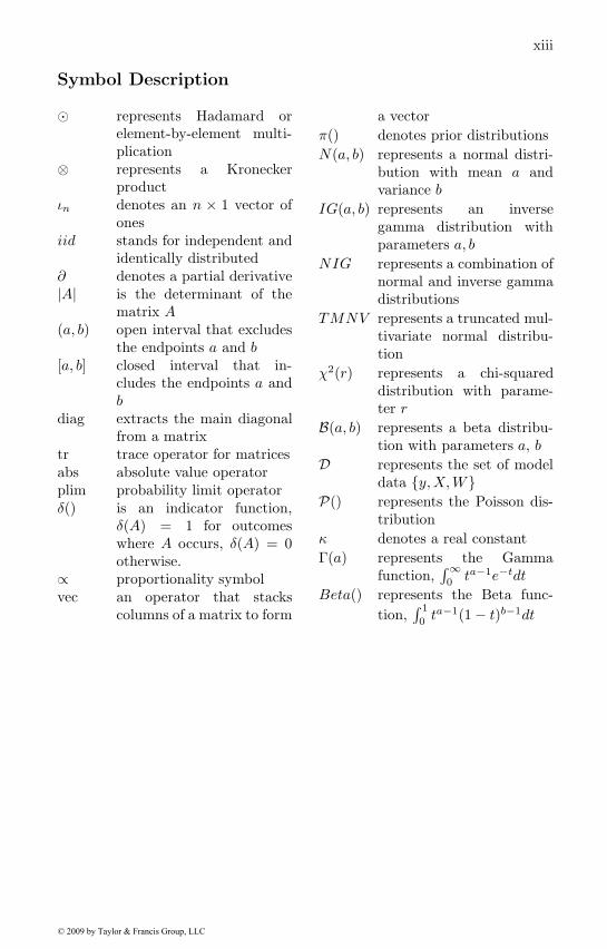
Symbol Description
� represents Hadamard orelement-by-element multi-plication
⊗ represents a Kroneckerproduct
ιn denotes an n × 1 vector ofones
iid stands for independent andidentically distributed
∂ denotes a partial derivative|A| is the determinant of the
matrix A(a, b) open interval that excludes
the endpoints a and b[a, b] closed interval that in-
cludes the endpoints a andb
diag extracts the main diagonalfrom a matrix
tr trace operator for matricesabs absolute value operatorplim probability limit operatorδ() is an indicator function,
δ(A) = 1 for outcomeswhere A occurs, δ(A) = 0otherwise.
∝ proportionality symbolvec an operator that stacks
columns of a matrix to form
a vectorπ() denotes prior distributionsN(a, b) represents a normal distri-
bution with mean a andvariance b
IG(a, b) represents an inversegamma distribution withparameters a, b
NIG represents a combination ofnormal and inverse gammadistributions
TMNV represents a truncated mul-tivariate normal distribu-tion
χ2(r) represents a chi-squareddistribution with parame-ter r
B(a, b) represents a beta distribu-tion with parameters a, b
D represents the set of modeldata {y,X,W}
P() represents the Poisson dis-tribution
κ denotes a real constantΓ(a) represents the Gamma
function,∫∞0 ta−1e−tdt
Beta() represents the Beta func-tion,
∫ 1
0 ta−1(1 − t)b−1dt
© 2009 by Taylor & Francis Group, LLC
Chapter 1
Introduction
Section 1.1 of this chapter introduces the concept of spatial dependence thatoften arises in cross-sectional spatial data samples. Spatial data samples rep-resent observations that are associated with points or regions, for examplehomes, counties, states, or census tracts. Two motivational examples are pro-vided for spatial dependence, one based on spatial spillovers stemming fromcongestion effects and a second that relies on omitted explanatory variables.Section 1.2 sets forth spatial autoregressive data generating processes for spa-tially dependent sample data along with spatial weight matrices that play animportant role in describing the structure of these processes. We provide moredetailed discussion of spatial data generating processes and associated spatialeconometric models in Chapter 2, and spatial weight matrices in Chapter 4.Our goal here is to provide an introduction to spatial autoregressive processesand spatial regression models that rely on this type of process. Section 1.3provides a simple example of how congestion effects lead to spatial spilloversthat impact neighboring regions using travel times to the central businessdistrict (CBD) region of a metropolitan area. Section 1.4 describes variousscenarios in which spatial econometric models can be used to analyze spatialspillover effects. The final section of the chapter lays out the plan of this text.A brief enumeration of the topics covered in each chapter is provided.
1.1 Spatial dependence
Consider a cross-sectional variable vector representing observations col-lected with reference to points or regions in space. Point observations couldinclude selling prices of homes, employment at various establishments, or en-rollment at individual schools. Geographic information systems typically sup-port geocoding or address matching which allow addresses to be automaticallyconverted into locational coordinates. The ability to geocode has led to vastamounts of spatially-referenced data. Observations could include a variablelike population or average commuting time for residents in regions such ascensus tracts, counties, or metropolitan statistical areas (MSAs). In contrastto point observations, for a region we rely on the coordinates of an interiorpoint representing the center (the centroid). An important point is that in
1© 2009 by Taylor & Francis Group, LLC
2 Introduction to Spatial Econometrics
spatial regression models each observation corresponds to a location or region.The data generating process (DGP) for a conventional cross-sectional non-
spatial sample of n independent observations yi, i = 1, . . . , n that are linearlyrelated to explanatory variables in a matrix X takes the form in (1.1), wherewe have suppressed the intercept term, which could be included in the matrixX .
yi = Xiβ + εi (1.1)εi ∼ N(0, σ2) i = 1, . . . , n (1.2)
In (1.2), we use N(a, b) to denote a univariate normal distribution with meana and variance b. In (1.1), Xi represents a 1 × k vector of covariates orexplanatory variables, with associated parameters β contained in a k × 1vector. This type of data generating process is typically assumed for linearregression models. Each observation has an underlying mean of Xiβ anda random component εi. An implication of this for situations where theobservations i represent regions or points in space is that observed valuesat one location (or region) are independent of observations made at otherlocations (or regions). Independent or statistically independent observationsimply that E(εiεj) = E(εi)E(εj) = 0. The assumption of independencegreatly simplifies models, but in spatial contexts this simplification seemsstrained.
In contrast, spatial dependence reflects a situation where values observed atone location or region, say observation i, depend on the values of neighboringobservations at nearby locations. Suppose we let observations i = 1 and j = 2represent neighbors (perhaps regions with borders that touch), then a datagenerating process might take the form shown in (1.3).
yi = αiyj +Xiβ + εi (1.3)yj = αjyi +Xjβ + εj
εi ∼ N(0, σ2) i = 1εj ∼ N(0, σ2) j = 2
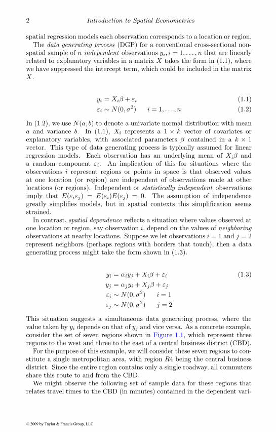
This situation suggests a simultaneous data generating process, where thevalue taken by yi depends on that of yj and vice versa. As a concrete example,consider the set of seven regions shown in Figure 1.1, which represent threeregions to the west and three to the east of a central business district (CBD).
For the purpose of this example, we will consider these seven regions to con-stitute a single metropolitan area, with region R4 being the central businessdistrict. Since the entire region contains only a single roadway, all commutersshare this route to and from the CBD.
We might observe the following set of sample data for these regions thatrelates travel times to the CBD (in minutes) contained in the dependent vari-
© 2009 by Taylor & Francis Group, LLC
Introduction 3
West East
R1 R2 R3 R4 R5 R6 R7
R1 R2 R3 R4 R5 R6 R7
CBD
CBD
Highway
FIGURE 1.1: Regions east and west of the Central Business District
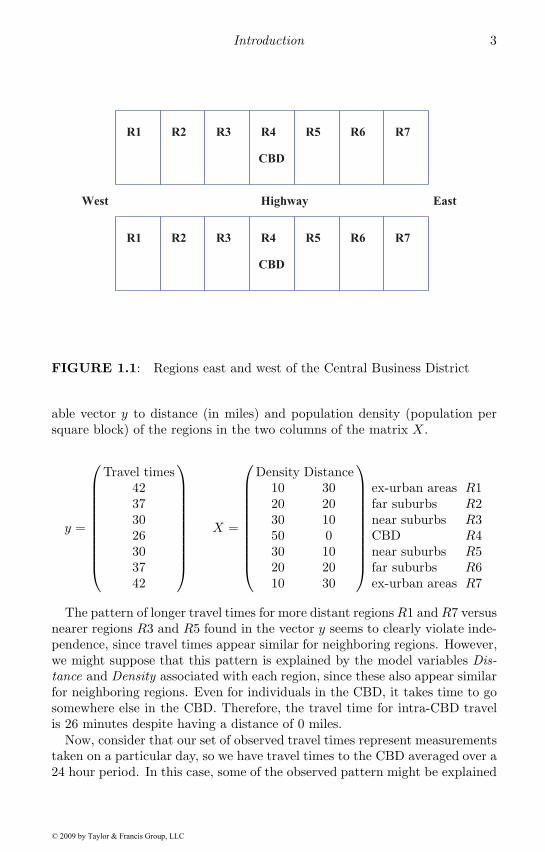
able vector y to distance (in miles) and population density (population persquare block) of the regions in the two columns of the matrix X .
y =
⎛⎜⎜⎜⎜⎜⎜⎜⎜⎜⎜⎝
Travel times42373026303742
⎞⎟⎟⎟⎟⎟⎟⎟⎟⎟⎟⎠X =
⎛⎜⎜⎜⎜⎜⎜⎜⎜⎜⎜⎝
Density Distance10 3020 2030 1050 030 1020 2010 30
⎞⎟⎟⎟⎟⎟⎟⎟⎟⎟⎟⎠
ex-urban areasfar suburbsnear suburbsCBDnear suburbsfar suburbsex-urban areas
R1R2R3R4R5R6R7
The pattern of longer travel times for more distant regionsR1 andR7 versusnearer regions R3 and R5 found in the vector y seems to clearly violate inde-pendence, since travel times appear similar for neighboring regions. However,we might suppose that this pattern is explained by the model variables Dis-tance and Density associated with each region, since these also appear similarfor neighboring regions. Even for individuals in the CBD, it takes time to gosomewhere else in the CBD. Therefore, the travel time for intra-CBD travelis 26 minutes despite having a distance of 0 miles.
Now, consider that our set of observed travel times represent measurementstaken on a particular day, so we have travel times to the CBD averaged over a24 hour period. In this case, some of the observed pattern might be explained
© 2009 by Taylor & Francis Group, LLC
4 Introduction to Spatial Econometrics
by congestion effects that arise from the shared highway. It seems plausiblethat longer travel times in one region should lead to longer travel times inneighboring regions on any given day. This is because commuters pass fromone region to another as they travel along the highway to the CBD. Slowertimes in R3 on a particular day should produce slower times for this day inregions R2 and R1. Congestion effects represent one type of spatial spillover,which do not occur simultaneously, but require some time for the traffic delayto arise. From a modeling viewpoint, congestion effects such as these will notbe explained by the model variables Distance and Density. These are dynamicfeedback effects from travel time on a particular day that impact travel timesof neighboring regions in the short time interval required for the traffic delay tooccur. Since the explanatory variable distance would not change from day today, and population density would change very slowly on a daily time scale,these variables would not be capable of explaining daily delay phenomena.Observed daily variation in travel times would be better explained by relyingon travel times from neighboring regions on that day. This is the situationdepicted in (1.3), where we rely on travel time from a neighboring observationyj as an explanatory variable for travel time in region i, yi. Similarly we useyi to explain region j travel time, yj .
Since our observations were measured using average times for one day, themeasurement time scale is not fine enough to capture the short-interval timedynamic aspect of traffic delay. This would result in observed daily traveltimes in the vector y that appear to be simultaneously determined. This is anexample of why measured spatial dependence may vary with the time-scale ofdata collection.
Another example where observed spatial dependence may arise from omit-ted variables would be the case of a hedonic pricing model with sales pricesof homes as the vector y and characteristics of the homes as explanatory vari-ables in the matrix X . If we have a cross-sectional sample of sales prices ina neighborhood collected over a period of one year, variation in the charac-teristics of the homes should explain part of the variation in observed salesprices. Consider a situation where a single home sells for a much higher pricethan would be expected based solely on its characteristics. Assume this saletook place at the mid-point of our 12 month observation period, shortly aftera positive school quality report was released for a nearby school. Since schoolquality was not a variable included in the set of explanatory variables rep-resenting home characteristics, the higher than expected selling price mightreflect a new premium for school quality. This might signal other sellers ofhomes served by the same school to ask for higher prices, or to accept of-fers that are much closer to their asking prices during the last six monthsof our observation period. This would lead to a situation where use of sell-ing prices from neighboring homes produce improved explanatory power forhomes served by the high quality school during the last six months of our sam-ple. Other omitted variables could be accessibility to transportation, nearbyamenities such as shopping or parks, and so on. If these were omitted from
© 2009 by Taylor & Francis Group, LLC
Introduction 5
the set of explanatory variables consisting solely of home characteristics, wewould find that selling prices from neighboring homes are useful for prediction.
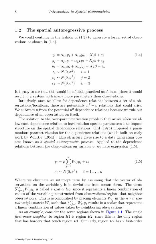
An illustration that non-spatial regression models will ignore spatial de-pendence in the dependent variable is provided by a map of the ordinaryleast-squares residuals from a production function regression: ln(Q) = αιn +β ln(K) + γ ln(L) + ε, estimated using the 48 contiguous US states plus theDistrict of Columbia. Gross state product for the year 2001 was used as Q,with labor L being 2001 total non-farm employment in each state. CapitalestimatesK for the states are from Garofalo and Yamarik (2002). These resid-uals are often referred to as the Solow residual if constant returns to scale areimposed so that β = φ, γ = (1 − φ). In the context of a Solow growth model,they are interpreted as reflecting economic growth above the rate of capitalgrowth, or that not explained by growth in factors of production. In the caseof our production function model, these would be interpreted as total factorproductivity, so they reflect output attributable to regional variation in thetechnological efficiency with which these factors are used.
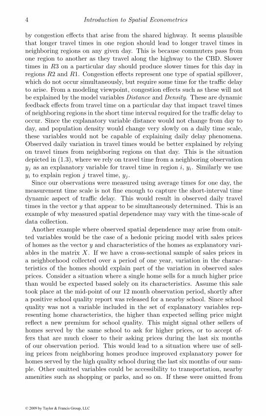
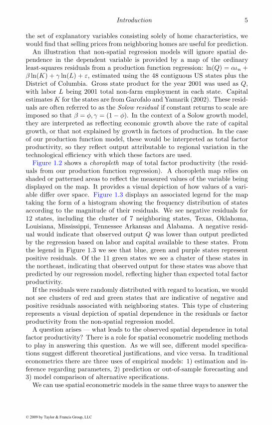
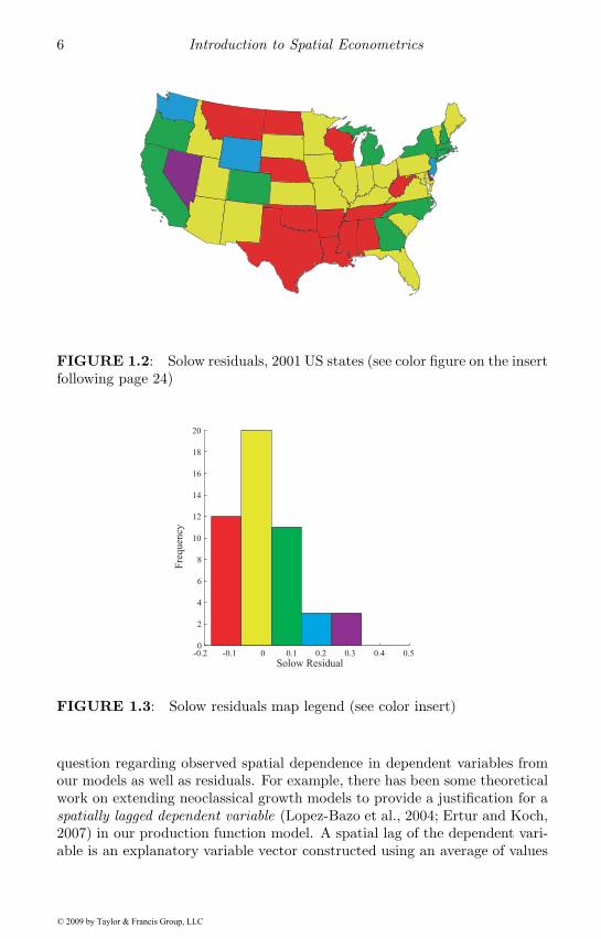
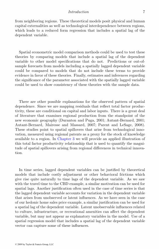
Figure 1.2 shows a choropleth map of total factor productivity (the resid-uals from our production function regression). A choropleth map relies onshaded or patterned areas to reflect the measured values of the variable beingdisplayed on the map. It provides a visual depiction of how values of a vari-able differ over space. Figure 1.3 displays an associated legend for the maptaking the form of a histogram showing the frequency distribution of statesaccording to the magnitude of their residuals. We see negative residuals for12 states, including the cluster of 7 neighboring states, Texas, Oklahoma,Louisiana, Mississippi, Tennessee Arkansas and Alabama. A negative resid-ual would indicate that observed output Q was lower than output predictedby the regression based on labor and capital available to these states. Fromthe legend in Figure 1.3 we see that blue, green and purple states representpositive residuals. Of the 11 green states we see a cluster of these states inthe northeast, indicating that observed output for these states was above thatpredicted by our regression model, reflecting higher than expected total factorproductivity.
If the residuals were randomly distributed with regard to location, we wouldnot see clusters of red and green states that are indicative of negative andpositive residuals associated with neighboring states. This type of clusteringrepresents a visual depiction of spatial dependence in the residuals or factorproductivity from the non-spatial regression model.
A question arises — what leads to the observed spatial dependence in totalfactor productivity? There is a role for spatial econometric modeling methodsto play in answering this question. As we will see, different model specifica-tions suggest different theoretical justifications, and vice versa. In traditionaleconometrics there are three uses of empirical models: 1) estimation and in-ference regarding parameters, 2) prediction or out-of-sample forecasting and3) model comparison of alternative specifications.
We can use spatial econometric models in the same three ways to answer the
© 2009 by Taylor & Francis Group, LLC
6 Introduction to Spatial Econometrics
FIGURE 1.2: Solow residuals, 2001 US states (see color figure on the insertfollowing page 24)
-0.2 -0.1 0 0.1 0.2 0.3 0.4 0.50
2
4
6
8
10
12
14
16
18
20
Solow Residual
Fre
qu
ency
FIGURE 1.3: Solow residuals map legend (see color insert)
question regarding observed spatial dependence in dependent variables fromour models as well as residuals. For example, there has been some theoreticalwork on extending neoclassical growth models to provide a justification for aspatially lagged dependent variable (Lopez-Bazo et al., 2004; Ertur and Koch,2007) in our production function model. A spatial lag of the dependent vari-able is an explanatory variable vector constructed using an average of values
© 2009 by Taylor & Francis Group, LLC
Introduction 7
from neighboring regions. These theoretical models posit physical and humancapital externalities as well as technological interdependence between regions,which leads to a reduced form regression that includes a spatial lag of thedependent variable.
Spatial econometric model comparison methods could be used to test thesetheories by comparing models that include a spatial lag of the dependentvariable to other model specifications that do not. Predictions or out-of-sample forecasts from models including a spatially lagged dependent variablecould be compared to models that do not include these terms to provideevidence in favor of these theories. Finally, estimates and inferences regardingthe significance of the parameter associated with the spatially lagged variablecould be used to show consistency of these theories with the sample data.
There are other possible explanations for the observed pattern of spatialdependence. Since we are mapping residuals that reflect total factor produc-tivity, these are conditional on capital and labor inputs. There is a great dealof literature that examines regional production from the standpoint of thenew economic geography (Duranton and Puga, 2001; Autant-Bernard, 2001;Autant-Bernard, Mairesse and Massard, 2007; Parent and LeSage, 2008).These studies point to spatial spillovers that arise from technological inno-vation, measured using regional patents as a proxy for the stock of knowledgeavailable to a region. In Chapter 3 we will provide an applied illustration ofthis total factor productivity relationship that is used to quantify the magni-tude of spatial spillovers arising from regional differences in technical innova-tion.
In time series, lagged dependent variables can be justified by theoreticalmodels that include costly adjustment or other behavioral frictions whichgive rise quite naturally to time lags of the dependent variable. As we sawwith the travel time to the CBD example, a similar motivation can be used forspatial lags. Another justification often used in the case of time series is thatthe lagged dependent variable accounts for variation in the dependent variablethat arises from unobserved or latent influences. As we have seen in the caseof our hedonic home sales price example, a similar justification can be used fora spatial lag of the dependent variable. Latent unobservable influences relatedto culture, infrastructure, or recreational amenities can affect the dependentvariable, but may not appear as explanatory variables in the model. Use of aspatial regression model that includes a spatial lag of the dependent variablevector can capture some of these influences.
© 2009 by Taylor & Francis Group, LLC
8 Introduction to Spatial Econometrics
1.2 The spatial autoregressive process
We could continue in the fashion of (1.3) to generate a larger set of obser-vations as shown in (1.4).
yi = αi,jyj + αi,kyk +Xiβ + εi (1.4)yj = αj,iyi + αj,kyk +Xjβ + εj
yk = αk,iyi + αk,jyj +Xkβ + εk
εi ∼ N(0, σ2) i = 1εj ∼ N(0, σ2) j = 2εk ∼ N(0, σ2) k = 3
It is easy to see that this would be of little practical usefulness, since it wouldresult in a system with many more parameters than observations.
Intuitively, once we allow for dependence relations between a set of n ob-servations/locations, there are potentially n2 − n relations that could arise.We subtract n from the potential n2 dependence relations because we rule outdependence of an observation on itself.
The solution to the over-parameterization problem that arises when we al-low each dependence relation to have relation-specific parameters is to imposestructure on the spatial dependence relations. Ord (1975) proposed a parsi-monious parameterization for the dependence relations (which built on earlywork by Whittle (1954)). This structure gives rise to a data generating pro-cess known as a spatial autoregressive process. Applied to the dependencerelations between the observations on variable y, we have expression (1.5).
yi = ρ
n∑j=1
Wijyj + εi (1.5)
εi ∼ N(0, σ2) i = 1, . . . , n
Where we eliminate an intercept term by assuming that the vector of ob-servations on the variable y is in deviations from means form. The term:∑n
j=1Wijyj is called a spatial lag, since it represents a linear combination ofvalues of the variable y constructed from observations/regions that neighborobservation i. This is accomplished by placing elements Wij in the n×n spa-tial weight matrix W , such that
∑nj=1Wijyj results in a scalar that represents
a linear combination of values taken by neighboring observations.As an example, consider the seven regions shown in Figure 1.1. The single
first-order neighbor to region R1 is region R2, since this is the only regionthat has borders that touch region R1. Similarly, region R2 has 2 first-order
© 2009 by Taylor & Francis Group, LLC
Introduction 9
neighbors, regions R1 and R3. We can define second-order neighbors as re-gions that are neighbors to the first-order neighbors. Second-order neighborsto region R1 would consist of all regions having borders that touch the first-order neighbor (region R2), which are: regions R1 and R3. It is importantto note that region R1 is a second-order neighbor to itself. This is becauseregion R1 is a neighbor to its neighbor, which is the definition of a second-order neighboring relation. If the neighboring relations are symmetric, eachregion will always be a second order neighbor to itself. By nature, contiguityrelations are symmetric, but we will discuss other definitions of neighboringrelations in Chapter 4 that may not result in symmetry.
We can write a matrix version of the spatial autoregressive process as in(1.6), where we use N(0, σ2In) to denote a zero mean disturbance process thatexhibits constant variance σ2, and zero covariance between observations. Thisresults in the diagonal variance-covariance matrix σ2In, where In representsan n-dimensional identity matrix. Expression (1.6) makes it clear that we aredescribing a relation between the vector y and the vector Wy representing alinear combination of neighboring values to each observation.
y = ρWy + ε (1.6)ε ∼ N(0, σ2In)
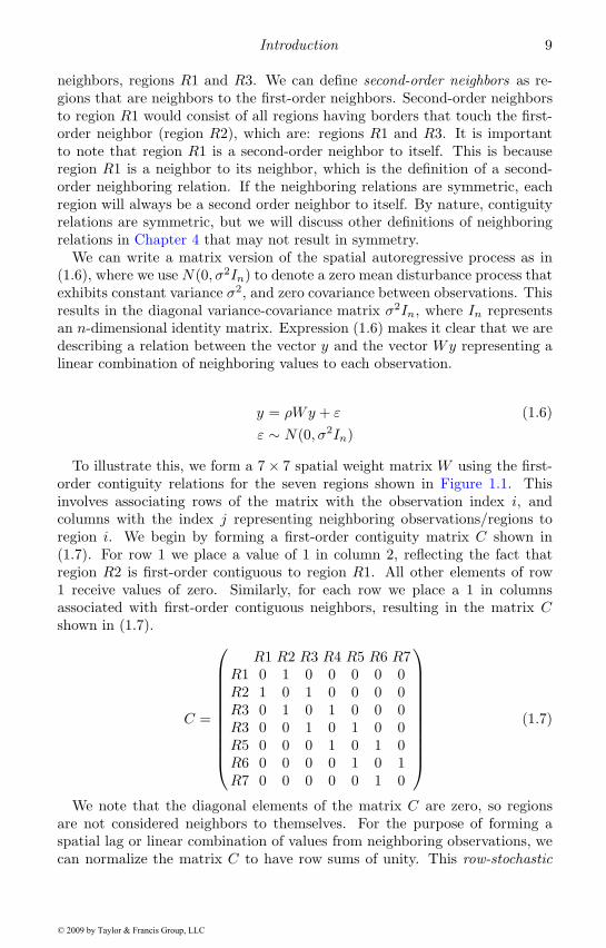
To illustrate this, we form a 7 × 7 spatial weight matrix W using the first-order contiguity relations for the seven regions shown in Figure 1.1. Thisinvolves associating rows of the matrix with the observation index i, andcolumns with the index j representing neighboring observations/regions toregion i. We begin by forming a first-order contiguity matrix C shown in(1.7). For row 1 we place a value of 1 in column 2, reflecting the fact thatregion R2 is first-order contiguous to region R1. All other elements of row1 receive values of zero. Similarly, for each row we place a 1 in columnsassociated with first-order contiguous neighbors, resulting in the matrix Cshown in (1.7).
C =
⎛⎜⎜⎜⎜⎜⎜⎜⎜⎜⎜⎝
R1 R2 R3 R4 R5 R6 R7R1 0 1 0 0 0 0 0R2 1 0 1 0 0 0 0R3 0 1 0 1 0 0 0R3 0 0 1 0 1 0 0R5 0 0 0 1 0 1 0R6 0 0 0 0 1 0 1R7 0 0 0 0 0 1 0
⎞⎟⎟⎟⎟⎟⎟⎟⎟⎟⎟⎠(1.7)
We note that the diagonal elements of the matrix C are zero, so regionsare not considered neighbors to themselves. For the purpose of forming aspatial lag or linear combination of values from neighboring observations, wecan normalize the matrix C to have row sums of unity. This row-stochastic
© 2009 by Taylor & Francis Group, LLC
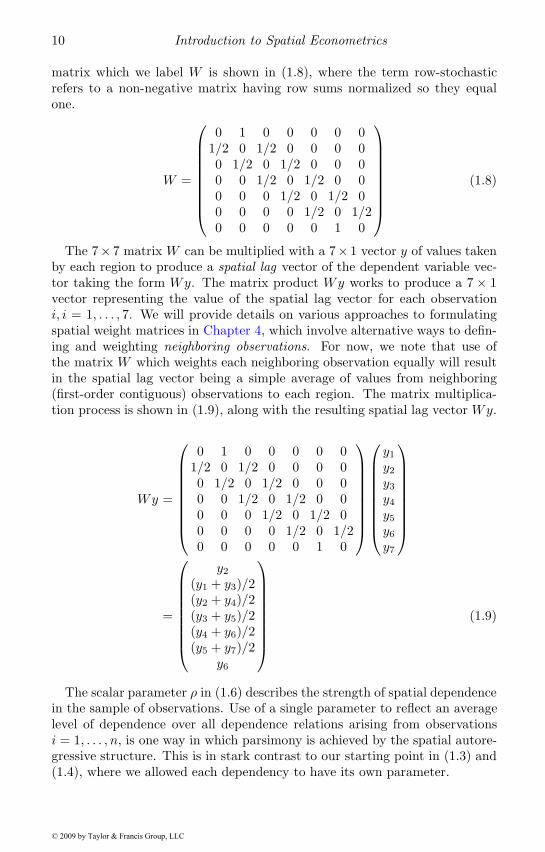
10 Introduction to Spatial Econometrics
matrix which we label W is shown in (1.8), where the term row-stochasticrefers to a non-negative matrix having row sums normalized so they equalone.
W =
⎛⎜⎜⎜⎜⎜⎜⎜⎜⎝
0 1 0 0 0 0 01/2 0 1/2 0 0 0 00 1/2 0 1/2 0 0 00 0 1/2 0 1/2 0 00 0 0 1/2 0 1/2 00 0 0 0 1/2 0 1/20 0 0 0 0 1 0
⎞⎟⎟⎟⎟⎟⎟⎟⎟⎠(1.8)
The 7× 7 matrix W can be multiplied with a 7× 1 vector y of values takenby each region to produce a spatial lag vector of the dependent variable vec-tor taking the form Wy. The matrix product Wy works to produce a 7 × 1vector representing the value of the spatial lag vector for each observationi, i = 1, . . . , 7. We will provide details on various approaches to formulatingspatial weight matrices in Chapter 4, which involve alternative ways to defin-ing and weighting neighboring observations. For now, we note that use ofthe matrix W which weights each neighboring observation equally will resultin the spatial lag vector being a simple average of values from neighboring(first-order contiguous) observations to each region. The matrix multiplica-tion process is shown in (1.9), along with the resulting spatial lag vector Wy.
Wy =
⎛⎜⎜⎜⎜⎜⎜⎜⎜⎝
0 1 0 0 0 0 01/2 0 1/2 0 0 0 00 1/2 0 1/2 0 0 00 0 1/2 0 1/2 0 00 0 0 1/2 0 1/2 00 0 0 0 1/2 0 1/20 0 0 0 0 1 0
⎞⎟⎟⎟⎟⎟⎟⎟⎟⎠
⎛⎜⎜⎜⎜⎜⎜⎜⎜⎝
y1y2y3y4y5y6y7
⎞⎟⎟⎟⎟⎟⎟⎟⎟⎠
=
⎛⎜⎜⎜⎜⎜⎜⎜⎜⎝
y2(y1 + y3)/2(y2 + y4)/2(y3 + y5)/2(y4 + y6)/2(y5 + y7)/2
y6
⎞⎟⎟⎟⎟⎟⎟⎟⎟⎠(1.9)
The scalar parameter ρ in (1.6) describes the strength of spatial dependencein the sample of observations. Use of a single parameter to reflect an averagelevel of dependence over all dependence relations arising from observationsi = 1, . . . , n, is one way in which parsimony is achieved by the spatial autore-gressive structure. This is in stark contrast to our starting point in (1.3) and(1.4), where we allowed each dependency to have its own parameter.
© 2009 by Taylor & Francis Group, LLC
Introduction 11
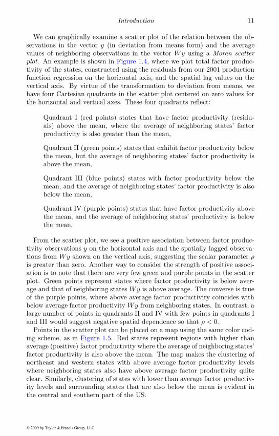
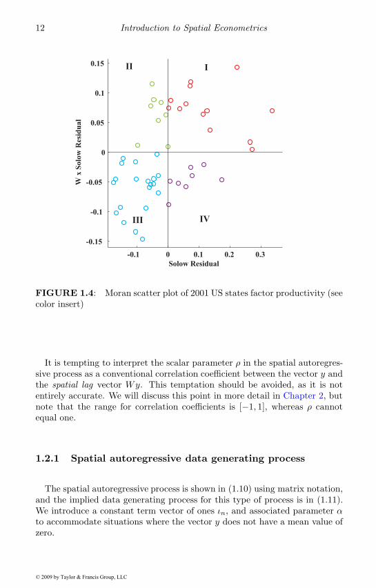
We can graphically examine a scatter plot of the relation between the ob-servations in the vector y (in deviation from means form) and the averagevalues of neighboring observations in the vector Wy using a Moran scatterplot. An example is shown in Figure 1.4, where we plot total factor produc-tivity of the states, constructed using the residuals from our 2001 productionfunction regression on the horizontal axis, and the spatial lag values on thevertical axis. By virtue of the transformation to deviation from means, wehave four Cartesian quadrants in the scatter plot centered on zero values forthe horizontal and vertical axes. These four quadrants reflect:
Quadrant I (red points) states that have factor productivity (residu-als) above the mean, where the average of neighboring states’ factorproductivity is also greater than the mean,
Quadrant II (green points) states that exhibit factor productivity belowthe mean, but the average of neighboring states’ factor productivity isabove the mean,
Quadrant III (blue points) states with factor productivity below themean, and the average of neighboring states’ factor productivity is alsobelow the mean,
Quadrant IV (purple points) states that have factor productivity abovethe mean, and the average of neighboring states’ productivity is belowthe mean.
From the scatter plot, we see a positive association between factor produc-tivity observations y on the horizontal axis and the spatially lagged observa-tions from Wy shown on the vertical axis, suggesting the scalar parameter ρis greater than zero. Another way to consider the strength of positive associ-ation is to note that there are very few green and purple points in the scatterplot. Green points represent states where factor productivity is below aver-age and that of neighboring states Wy is above average. The converse is trueof the purple points, where above average factor productivity coincides withbelow average factor productivity Wy from neighboring states. In contrast, alarge number of points in quadrants II and IV with few points in quadrants Iand III would suggest negative spatial dependence so that ρ < 0.
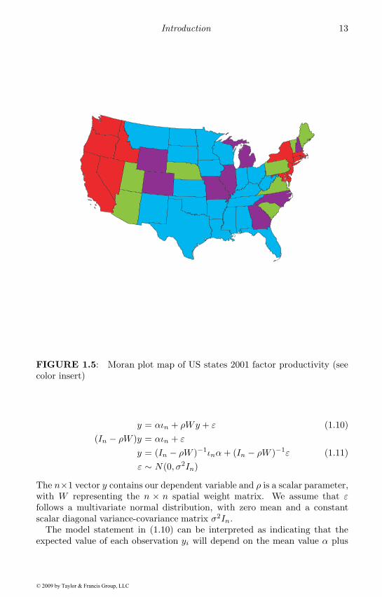
Points in the scatter plot can be placed on a map using the same color cod-ing scheme, as in Figure 1.5. Red states represent regions with higher thanaverage (positive) factor productivity where the average of neighboring states’factor productivity is also above the mean. The map makes the clustering ofnortheast and western states with above average factor productivity levelswhere neighboring states also have above average factor productivity quiteclear. Similarly, clustering of states with lower than average factor productiv-ity levels and surrounding states that are also below the mean is evident inthe central and southern part of the US.
© 2009 by Taylor & Francis Group, LLC
12 Introduction to Spatial Econometrics
-0.1 0 0.1 0.2 0.3
-0.15
-0.1
-0.05
0
0.05
0.1
0.15
Solow Residual
W x
So
low
Res
idu
al
III
III IV
FIGURE 1.4: Moran scatter plot of 2001 US states factor productivity (seecolor insert)
It is tempting to interpret the scalar parameter ρ in the spatial autoregres-sive process as a conventional correlation coefficient between the vector y andthe spatial lag vector Wy. This temptation should be avoided, as it is notentirely accurate. We will discuss this point in more detail in Chapter 2, butnote that the range for correlation coefficients is [−1, 1], whereas ρ cannotequal one.
1.2.1 Spatial autoregressive data generating process
The spatial autoregressive process is shown in (1.10) using matrix notation,and the implied data generating process for this type of process is in (1.11).We introduce a constant term vector of ones ιn, and associated parameter αto accommodate situations where the vector y does not have a mean value ofzero.
© 2009 by Taylor & Francis Group, LLC
Introduction 13
FIGURE 1.5: Moran plot map of US states 2001 factor productivity (seecolor insert)
y = αιn + ρWy + ε (1.10)(In − ρW )y = αιn + ε
y = (In − ρW )−1ιnα+ (In − ρW )−1ε (1.11)ε ∼ N(0, σ2In)
The n×1 vector y contains our dependent variable and ρ is a scalar parameter,with W representing the n × n spatial weight matrix. We assume that εfollows a multivariate normal distribution, with zero mean and a constantscalar diagonal variance-covariance matrix σ2In.
The model statement in (1.10) can be interpreted as indicating that theexpected value of each observation yi will depend on the mean value α plus
© 2009 by Taylor & Francis Group, LLC
14 Introduction to Spatial Econometrics
a linear combination of values taken by neighboring observations scaled bythe dependence parameter ρ. The data generating process statement in (1.11)expresses the simultaneous nature of the spatial autoregressive process. Tofurther explore the nature of this, we can use the following infinite series toexpress the inverse:
(In − ρW )−1 = In + ρW + ρ2W 2 + ρ3W 3 + . . . (1.12)
where we assume for the moment that abs(ρ) < 1. This leads to a spatialautoregressive data generating process for a variable vector y:
y = (In − ρW )−1ιnα+ (In − ρW )−1ε
y = αιn + ρWιnα+ ρ2W 2ιnα+ . . .
+ ε+ ρWε+ ρ2W 2ε+ ρ3W 3ε+ . . . (1.13)
Expression (1.13) can be simplified since the infinite series: ιnα+ρWιnα+ρ2W 2ιnα + . . . converges to (1 − ρ)−1ιnα since α is a scalar, the parameterabs(ρ) < 1, and W is row-stochastic. By definition, Wιn = ιn and thereforeW (Wιn) also equals Wιn = ιn. Consequently, W qιn = ιn for q ≥ 0 (recallthat W 0 = In). This allows us to write:
y =1
(1 − ρ)ιnα+ ε+ ρWε+ ρ2W 2ε+ ρ3W 3ε+ . . . (1.14)
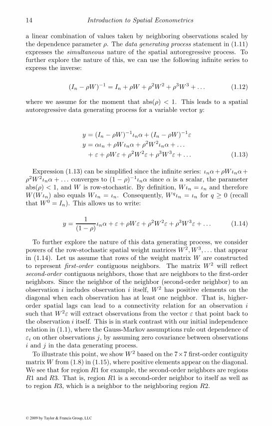
To further explore the nature of this data generating process, we considerpowers of the row-stochastic spatial weight matrices W 2,W 3, . . . that appearin (1.14). Let us assume that rows of the weight matrix W are constructedto represent first-order contiguous neighbors. The matrix W 2 will reflectsecond-order contiguous neighbors, those that are neighbors to the first-orderneighbors. Since the neighbor of the neighbor (second-order neighbor) to anobservation i includes observation i itself, W 2 has positive elements on thediagonal when each observation has at least one neighbor. That is, higher-order spatial lags can lead to a connectivity relation for an observation isuch that W 2ε will extract observations from the vector ε that point back tothe observation i itself. This is in stark contrast with our initial independencerelation in (1.1), where the Gauss-Markov assumptions rule out dependence ofεi on other observations j, by assuming zero covariance between observationsi and j in the data generating process.
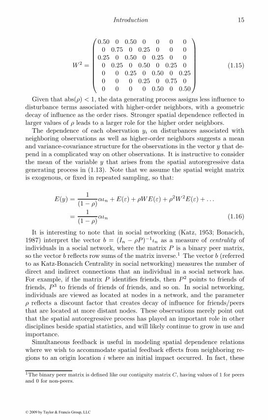
To illustrate this point, we show W 2 based on the 7×7 first-order contiguitymatrixW from (1.8) in (1.15), where positive elements appear on the diagonal.We see that for region R1 for example, the second-order neighbors are regionsR1 and R3. That is, region R1 is a second-order neighbor to itself as well asto region R3, which is a neighbor to the neighboring region R2.
© 2009 by Taylor & Francis Group, LLC
Introduction 15
W 2 =
⎛⎜⎜⎜⎜⎜⎜⎜⎜⎝
0.50 0 0.50 0 0 0 00 0.75 0 0.25 0 0 0
0.25 0 0.50 0 0.25 0 00 0.25 0 0.50 0 0.25 00 0 0.25 0 0.50 0 0.250 0 0 0.25 0 0.75 00 0 0 0 0.50 0 0.50
⎞⎟⎟⎟⎟⎟⎟⎟⎟⎠(1.15)
Given that abs(ρ) < 1, the data generating process assigns less influence todisturbance terms associated with higher-order neighbors, with a geometricdecay of influence as the order rises. Stronger spatial dependence reflected inlarger values of ρ leads to a larger role for the higher order neighbors.
The dependence of each observation yi on disturbances associated withneighboring observations as well as higher-order neighbors suggests a meanand variance-covariance structure for the observations in the vector y that de-pend in a complicated way on other observations. It is instructive to considerthe mean of the variable y that arises from the spatial autoregressive datagenerating process in (1.13). Note that we assume the spatial weight matrixis exogenous, or fixed in repeated sampling, so that:
E(y) =1
(1 − ρ)αιn + E(ε) + ρWE(ε) + ρ2W 2E(ε) + . . .
=1
(1 − ρ)αιn (1.16)
It is interesting to note that in social networking (Katz, 1953; Bonacich,1987) interpret the vector b = (In − ρP )−1ιn as a measure of centrality ofindividuals in a social network, where the matrix P is a binary peer matrix,so the vector b reflects row sums of the matrix inverse.1 The vector b (referredto as Katz-Bonacich Centrality in social networking) measures the number ofdirect and indirect connections that an individual in a social network has.For example, if the matrix P identifies friends, then P 2 points to friends offriends, P 3 to friends of friends of friends, and so on. In social networking,individuals are viewed as located at nodes in a network, and the parameterρ reflects a discount factor that creates decay of influence for friends/peersthat are located at more distant nodes. These observations merely point outthat the spatial autoregressive process has played an important role in otherdisciplines beside spatial statistics, and will likely continue to grow in use andimportance.
Simultaneous feedback is useful in modeling spatial dependence relationswhere we wish to accommodate spatial feedback effects from neighboring re-gions to an origin location i where an initial impact occurred. In fact, these
1The binary peer matrix is defined like our contiguity matrix C, having values of 1 for peersand 0 for non-peers.
© 2009 by Taylor & Francis Group, LLC
16 Introduction to Spatial Econometrics
models allow us to treat all observations as potential origins of an impactwithout loss of generality. One might suppose that feedback effects wouldtake time, but there is no explicit role for passage of time in a cross-sectionalrelation. Instead, we can view the cross-sectional sample data observationsas reflecting an equilibrium outcome or steady state of the spatial process weare modeling. We develop this idea further in Chapter 2 and Chapter 7. Thisis an interpretation often used in cross-sectional modeling and Sen and Smith(1995) provide examples of this type of situation for conventional spatial in-teraction models used in regional analysis. The goal in spatial interactionmodels is to analyze variation in flows between regions that occur over timeusing a cross-section of observed flows between origin and destination regionsthat have taken place over a finite period of time, but measured at a singlepoint in time. We discuss spatial econometric models for origin-destinationflows in Chapter 8.
This simultaneous dependence situation does not occur in time series anal-ysis, making spatial autoregressive processes distinct from time series autore-gressive processes. In time series, the time lag operator L is strictly triangularand contains zeros on the diagonal. Powers of L are also strictly triangularwith zeros on the diagonal, so that L2 specifies a two-period time lag whereasL creates a single period time lag. It is never the case that L2 producesobservations that point back to include the present time period.
1.3 An illustration of spatial spillovers
The spatial autoregressive structure can be combined with a conventionalregression model to produce a spatial extension of the standard regressionmodel shown in (1.17), with the implied data generating process in (1.18). Wewill refer to this as simply the spatial autoregressive model (SAR) throughoutthe text. We note that Anselin (1988) labeled this model a “mixed-regressive,spatial-autoregressive” model, where the motivation for this awkward nomen-clature should be clear.
y = ρWy +Xβ + ε (1.17)y = (In − ρW )−1Xβ + (In − ρW )−1ε (1.18)ε ∼ N(0, σ2In)
In this model, the parameters to be estimated are the usual regressionparameters β, σ and the additional parameter ρ. It is noteworthy that if thescalar parameter ρ takes a value of zero so there is no spatial dependencein the vector of cross-sectional observations y, this yields the least-squaresregression model as a special case of the SAR model.
© 2009 by Taylor & Francis Group, LLC
Introduction 17
To provide an illustration of how the spatial regression model can be usedto quantify spatial spillovers, we reuse the earlier example of travel times tothe CBD from the seven regions shown in Figure 1.1. We consider the impactof a change in population density for a single region on travel times to theCBD for all seven regions. Specifically, we double the population density inregion R2 and make a prediction of the impact on travel times to the CBDfor all seven regions.
We use parameter estimates: β′ =[0.135 0.561
]and ρ = 0.642 for this
example. The estimated value of ρ indicates positive spatial dependence incommuting times. Predictions from the model based on the explanatory vari-ables matrix X would take the form:
y(1) = (In − ρW )−1Xβ
where ρ, β are maximum likelihood estimates.A comparison of predictions y(1) from the model with explanatory variables
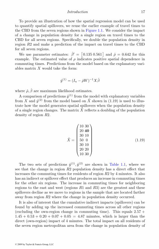
from X and y(2) from the model based on X shown in (1.19) is used to illus-trate how the model generates spatial spillovers when the population densityof a single region changes. The matrix X reflects a doubling of the populationdensity of region R2.
X =
⎛⎜⎜⎜⎜⎜⎜⎜⎜⎝
10 3020 4030 1050 030 1020 2010 30
⎞⎟⎟⎟⎟⎟⎟⎟⎟⎠(1.19)
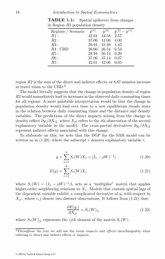
The two sets of predictions y(1), y(2) are shown in Table 1.1, where wesee that the change in region R2 population density has a direct effect thatincreases the commuting times for residents of region R2 by 4 minutes. It alsohas an indirect or spillover effect that produces an increase in commuting timesfor the other six regions. The increase in commuting times for neighboringregions to the east and west (regions R1 and R3) are the greatest and thesespillovers decline as we move to regions in the sample that are located fartheraway from region R2 where the change in population density occurred.
It is also of interest that the cumulative indirect impacts (spillovers) can befound by adding up the increased commuting times across all other regions(excluding the own-region change in commuting time). This equals 2.57 +1.45 + 0.53 + 0.20 + 0.07 + 0.05 = 4.87 minutes, which is larger than thedirect (own-region) impact of 4 minutes. The total impact on all residents ofthe seven region metropolitan area from the change in population density of
© 2009 by Taylor & Francis Group, LLC
18 Introduction to Spatial Econometrics
TABLE 1.1: Spatial spillovers from changesin Region R2 population density
Regions / Scenario y(1) y(2) y(2) − y(1)
R1 : 42.01 44.58 2.57R2 : 37.06 41.06 4.00R3 : 29.94 31.39 1.45R4 : CBD 26.00 26.54 0.53R5 : 29.94 30.14 0.20R6 : 37.06 37.14 0.07R7 : 42.01 42.06 0.05
region R2 is the sum of the direct and indirect effects, or 8.87 minutes increasein travel times to the CBD.2
The model literally suggests that the change in population density of regionR2 would immediately lead to increases in the observed daily commuting timesfor all regions. A more palatable interpretation would be that the change inpopulation density would lead over time to a new equilibrium steady statein the relation between daily commuting times and the distance and densityvariables. The predictions of the direct impacts arising from the change indensity reflect ∂yi/∂Xi2, where Xi2 refers to the ith observation of the secondexplanatory variable in the model. The cross-partial derivatives ∂yj/∂Xi2
represent indirect effects associated with this change.To elaborate on this, we note that the DGP for the SAR model can be
written as in (1.20), where the subscript r denotes explanatory variable r,
y =k∑r=1
Sr(W )Xr + (In − ρW )−1ε (1.20)
E(y) =k∑r=1
Sr(W )Xr (1.21)
where Sr(W ) = (In − ρW )−1βr acts as a “multiplier” matrix that applieshigher-order neighboring relations to Xr. Models that contain spatial lags ofthe dependent variable exhibit a complicated derivative of yi with respect toXjr , where i, j denote two distinct observations. It follows from (1.21) that:
∂E(yi)∂Xjr
= Sr(W )ij (1.22)
where Sr(W )ij represents the ijth element of the matrix Sr(W ).
2Throughout the text we will use the terms impacts and effects interchangeably whenreferring to direct and indirect effects or impacts.
© 2009 by Taylor & Francis Group, LLC
Introduction 19
As expression (1.22) indicates, the standard regression interpretation ofcoefficient estimates as partial derivatives: βr = ∂y/∂Xr, no longer holds.Because of the transformation of Xr by the n× n matrix Sr(W ), any changeto an explanatory variable in a given region (observation) can affect the de-pendent variable in all regions (observations) through the matrix inverse.
Since the impact of changes in an explanatory variable differ over all obser-vations, it seems desirable to find a summary measure for the own derivative∂yi/∂Xir in (1.22) that shows the impact arising from a change in the ithobservation of variable r. It would also be of interest to summarize the crossderivative ∂yi/∂Xjr(i �= j) in (1.22) that measures the impact on yi fromchanges in observation j of variable r. We pursue this topic in detail in Chap-ter 2, where we provide summary measures and interpretations for the impactsthat arise from changes represented by the own- and cross-partial derivatives.
Despite the simplicity of this example, it provides an illustration of howspatial regression models allow for spillovers from changes in the explanatoryvariables of a single region in the sample. This is a valuable aspect of spatialeconometric models that sets them apart from most spatial statistical models,an issue we discuss in the next section.
An ordinary regression model would make the prediction that the change inpopulation density in region R2 affects only the commuting time of residentsin region R2, with no allowance for spatial spillover impacts. To see this, wecan set the parameter ρ = 0 in our model, which produces the non-spatialregression model. In this case y(1) = Xβo and y(2) = Xβo, so the differencewould be Xβo−Xβo = (X−X)βo, where the estimated parameters βo wouldbe those from a least-squares regression.
If the DGP for our observed daily travel times is that of the SAR model,least-squares estimates will be biased and inconsistent, since they ignore thespatial lag of the dependent variable. To see this, note that the estimates forβ from the SAR model take the form: β = (X ′X)−1X ′(In − ρW )y, a subjectwe pursue in more detail in Chapter 2. For our simple illustration where allvalues of y and X are positive, and the spatial dependence parameter is alsopositive, this suggests an upward bias in the least-squares estimates. This canbe seen by noting that:
β = (X ′X)−1X ′y − ρ(X ′X)−1X ′Wy
β = βo − ρ(X ′X)−1X ′Wy
βo = β + ρ(X ′X)−1X ′Wy
Since all values of y are positive, the spatial lag vector Wy will containaverages of the neighboring values which will also be positive. This in con-junction with only positive elements in the matrix X as well as positive ρlead us to conclude that the least-squares estimates βo will be biased upwardrelative to the unbiased estimates β. For our seven region example, the least-squares estimates were: β′
o =[0.55 1.25
], which show upward bias relative to
© 2009 by Taylor & Francis Group, LLC
20 Introduction to Spatial Econometrics
the spatial autoregressive model estimates: β′ =[0.135 0.561
]. Intuitively,
the ordinary least-squares model attempts to explain variation in travel timesthat arises from spillover congestion effects using the distance and populationdensity variables. This results in an overstatement of the true influence ofthese variables on travel times.
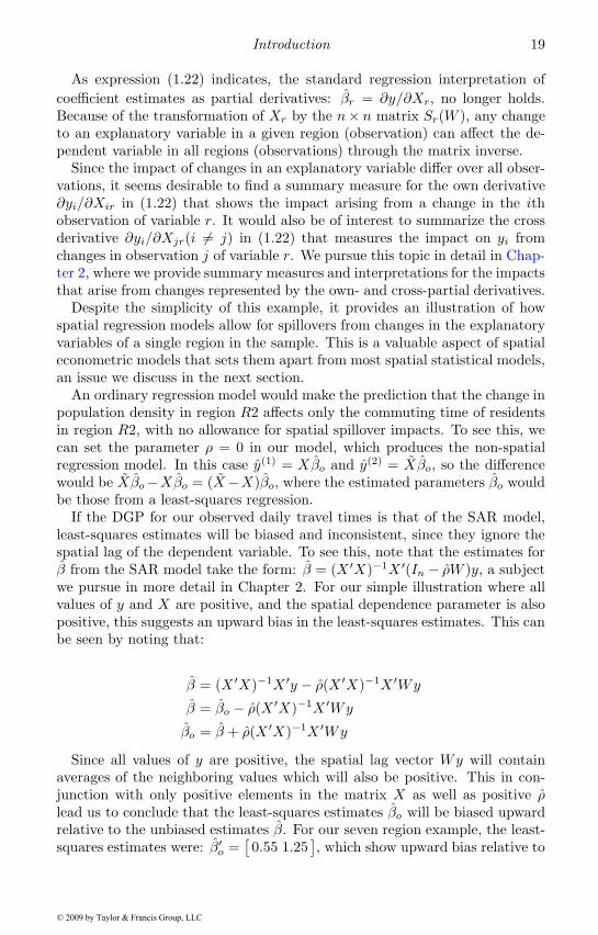
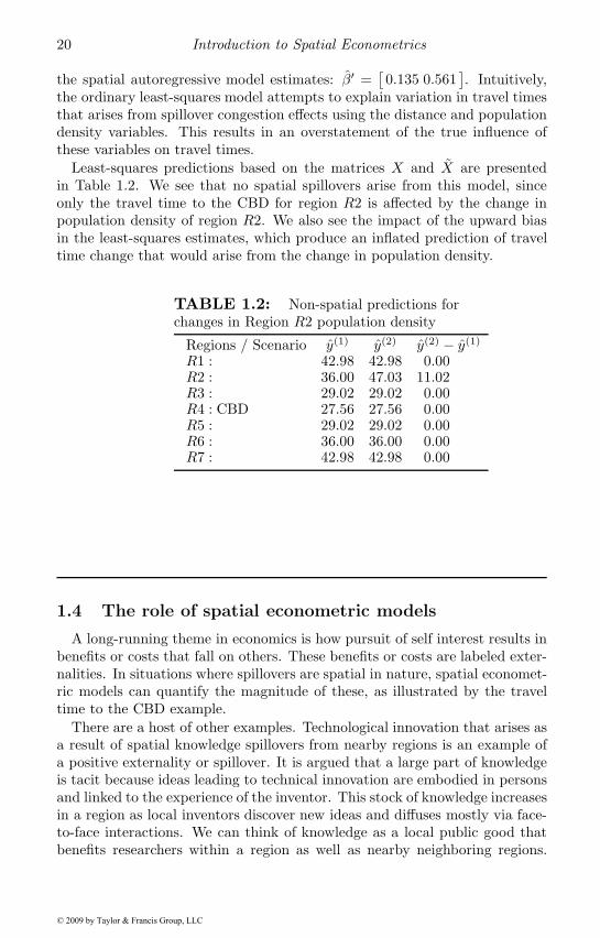
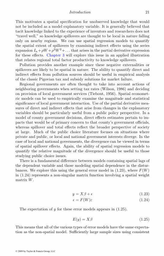
Least-squares predictions based on the matrices X and X are presentedin Table 1.2. We see that no spatial spillovers arise from this model, sinceonly the travel time to the CBD for region R2 is affected by the change inpopulation density of region R2. We also see the impact of the upward biasin the least-squares estimates, which produce an inflated prediction of traveltime change that would arise from the change in population density.
TABLE 1.2: Non-spatial predictions forchanges in Region R2 population density
Regions / Scenario y(1) y(2) y(2) − y(1)
R1 : 42.98 42.98 0.00R2 : 36.00 47.03 11.02R3 : 29.02 29.02 0.00R4 : CBD 27.56 27.56 0.00R5 : 29.02 29.02 0.00R6 : 36.00 36.00 0.00R7 : 42.98 42.98 0.00
1.4 The role of spatial econometric models
A long-running theme in economics is how pursuit of self interest results inbenefits or costs that fall on others. These benefits or costs are labeled exter-nalities. In situations where spillovers are spatial in nature, spatial economet-ric models can quantify the magnitude of these, as illustrated by the traveltime to the CBD example.
There are a host of other examples. Technological innovation that arises asa result of spatial knowledge spillovers from nearby regions is an example ofa positive externality or spillover. It is argued that a large part of knowledgeis tacit because ideas leading to technical innovation are embodied in personsand linked to the experience of the inventor. This stock of knowledge increasesin a region as local inventors discover new ideas and diffuses mostly via face-to-face interactions. We can think of knowledge as a local public good thatbenefits researchers within a region as well as nearby neighboring regions.
© 2009 by Taylor & Francis Group, LLC
Introduction 21
This motivates a spatial specification for unobserved knowledge that wouldnot be included as a model explanatory variable. It is generally believed thattacit knowledge linked to the experience of inventors and researchers does not“travel well,” so knowledge spillovers are thought to be local in nature fallingonly on nearby regions. We can use spatial regression models to quantifythe spatial extent of spillovers by examining indirect effects using the seriesexpansion In+ρW+ρ2W 2+ . . . that arises in the partial derivative expressionfor these effects. Chapter 3 will explore this issue in an applied illustrationthat relates regional total factor productivity to knowledge spillovers.
Pollution provides another example since these negative externalities orspillovers are likely to be spatial in nature. The ability to quantify direct andindirect effects from pollution sources should be useful in empirical analysisof the classic Pigovian tax and subsidy solutions for market failure.
Regional governments are often thought to take into account actions ofneighboring governments when setting tax rates (Wilson, 1986) and decidingon provision of local government services (Tiebout, 1956). Spatial economet-ric models can be used to empirically examine the magnitude and statisticalsignificance of local government interaction. Use of the partial derivative mea-sures of direct and indirect effects that arise from changes in the explanatoryvariables should be particularly useful from a public policy perspective. In amodel of county government decisions, direct effects estimates pertain to im-pacts that would be of primary concern to that county’s government officials,whereas spillover and total effects reflect the broader perspective of societyat large. Much of the public choice literature focuses on situations whereprivate and public, or local and national government interests diverge. In thecase of local and national governments, the divergence can be viewed in termsof spatial spillover effects. Again, the ability of spatial regression models toquantify the relative magnitude of the divergence should be useful to thosestudying public choice issues.
There is a fundamental difference between models containing spatial lags ofthe dependent variable and those modeling spatial dependence in the distur-bances. We explore this using the general error model in (1.23), where F (W )in (1.24) represents a non-singular matrix function involving a spatial weightmatrix W .
y = Xβ + ε (1.23)ε = F (W )ε (1.24)
The expectation of y for these error models appears in (1.25).
E(y) = Xβ (1.25)
This means that all of the various types of error models have the same expecta-tion as the non-spatial model. Sufficiently large sample sizes using consistent
© 2009 by Taylor & Francis Group, LLC
22 Introduction to Spatial Econometrics
estimators on the various models should yield identical estimates of the pa-rameters β. For small samples the estimates could vary, and using modelsthat differ from the DGP could lead to inconsistent estimates of dispersionfor the model parameters. Interpretation of the parameters β from this typeof model is the same as for a non-spatial linear regression model.
Anselin (1988) provides a persuasive argument that the focus of spatialeconometrics should be on measuring the effects of spillovers. We pay limitedattention to error models in this text because these models eliminate spilloversby construction. These could be added by making X more spatially complex,but there are more appealing alternatives that we will explore here.
1.5 The plan of the text
This introductory chapter focused on a brief introduction to spatial depen-dence and spatial autoregressive processes, as well as spatial weight matricesused in these processes. These processes can be used to produce a host of spa-tial econometric models that accommodate spatial dependence taking variousforms.
Chapter 2 provides more detailed motivations for spatial dependence andthe use of spatial regression models. We elaborate on the idea that omitted orexcluded variables in our models that exhibit spatial dependence can lead tospatial regression models that contain spatial lags of the dependent variable.Cross-sectional simultaneous spatial regression models are also motivated asa long-run steady-state outcome of non-simultaneous dependence situations.We consider situations where economic agents can observe past actions ofneighboring agents, for example county government officials should be awareof neighboring government tax rates or levels of government services provisionin the previous period. This type of non-simultaneous space-time dynamicrelationship is consistent with a cross-sectional simultaneous spatial regressionrelationship that represents the long-run steady state outcome of the space-time dynamic relationship. We also provide details regarding interpretationof estimates from these models. An elaboration is provided regarding directand indirect effects associated with changes in explanatory variables that wasintroduced in the travel time example of this chapter.
Chapter 3 will focus on a family of spatial regression models popularized byAnselin (1988) in his influential text on spatial econometrics. The implicationsfor estimates and inferences based on least-squares estimates from non-spatialregression in the presence of spatial dependence are discussed. This chapteralso provides details regarding computational aspects of maximum likelihoodestimation for the family of spatial regression models. Computational meth-ods have advanced considerably since 1988, the year of Anselin’s text.
© 2009 by Taylor & Francis Group, LLC
Introduction 23
Chapter 4 addresses various computational and theoretical aspects of spa-tial econometric models. Topics include computation of spatial weight ma-trices, log-determinants (including numerous special cases such as the matrixexponential, equation systems, multiple weight matrices, and flow matrices),derivatives of log-determinants, diagonals of the variance-covariance matrix,and closed-form solutions for a number of single-parameter spatial models.
Conventional Bayesian methods for analyzing spatial econometric models(Anselin, 1988; Hepple, 1995a,b) as well as more recent Bayesian MarkovChain Monte Carlo (MCMC) methods (LeSage, 1997) for estimating spatialregression models are the subject of Chapter 5. The approach set forth inLeSage (1997) allows formal treatment of spatial heterogeneity that is mo-tivated in Chapter 2. We show that many of the computational advancesdescribed for maximum likelihood estimation in Chapter 3 also work to sim-plify Bayesian estimation of these models.
Model specification and comparison is the topic of Chapter 6. Specificationissues considered include the form of the weight matrix, the usual concernabout appropriate explanatory variables, and questions regarding which ofthe alternative members of the family of spatial regression models introducedin Chapter 3 should be employed. We show how formal Bayesian modelcomparison methods proposed by LeSage and Parent (2007) can be used toanswer questions regarding appropriate explanatory variables for the family ofmodels from Chapter 3. Bayesian model comparison methods can also be usedto discriminate between models based on alternative spatial weight matricesas noted by LeSage and Pace (2004a) and different specifications arising fromthe family of spatial regression models from Chapter 3 (Hepple, 2004).
Chapter 7 is unlike other chapters in the text since it is more theoreti-cal, focusing on spatiotemporal foundations for observed cross-sectional spa-tial dependence. Starting with the assumption that regions are influencedonly by own and other regions past period values we develop a spatiotem-poral motivation for simultaneous spatial dependence implied by the spatialautoregressive process. We elaborate on the discussion in Chapter 2 show-ing how time dependence on past decisions of neighboring economic agentswill lead to simultaneous spatial regression specifications. We show that astrict spatiotemporal framework consistent with a spatial partial adjustmentmechanism can result in a long-run equilibrium characterized by simultaneousspatial dependence.
Spatial econometric extensions of conventional least-squares gravity or spa-tial interaction models described in Sen and Smith (1995) are the topic ofChapter 8. We present spatial regression models similar to those from Chap-ter 3 introduced by LeSage and Pace (2008) that can be applied to modelsthat attempt to explain variation in flows between origins and destinations.Allowing for spatial dependence at origins, destinations, and between originsand destinations leads to a situation where changes at either the origin ordestination will give rise to forces that set in motion a series of events. Weexplore the notion advanced by Behrens, Ertur and Koch (2007) that spatial
© 2009 by Taylor & Francis Group, LLC
24 Introduction to Spatial Econometrics
dependence suggests a multilateral world where indirect interactions link allregions. This contrasts with conventional emphasis on bilateral flows fromorigin to destination regions.
Chapter 9 sets forth an alternative approach for spatial econometric model-ing that replaces the spatial autoregressive process with a matrix exponentialapproach to specifying spatial dependence structures (LeSage and Pace, 2007,2004b). This has both computational as well as theoretical advantages overthe more conventional spatial autoregressive process. We discuss both maxi-mum likelihood and Bayesian approaches to estimating models based on thisnew spatial process specification.
Chapter 10 takes up the topic of spatial regressions involving binary, countor truncated dependent variables. This draws on work regarding binary de-pendent variables in the context of the family of models from Chapter 3described in LeSage (2000) and surveyed by Flemming (2004). Use of spatialautoregressive processes as a Bayesian prior for spatially structured effectsintroduced in Smith and LeSage (2004) for the case of probit models andin LeSage, Fischer and Scherngell (2007) for Poisson count data models arealso discussed. This approach to structuring individual effects parameters canbe used to overcome problems that typically arise when estimating individ-ual effects (Christensen, Roberts and Skold, 2006; Gelfand, Sahu and Carlin,1995).
© 2009 by Taylor & Francis Group, LLC
Chapter 2
Motivating and Interpreting SpatialEconometric Models
In the first five sections of this chapter, we provide separate motivations forregression models that include spatial autoregressive processes. These moti-vations are explored in more detail in later chapters of the text, with the pre-sentation here being less formal. Section 2.1 shows how cross-sectional modelrelations involving spatial lags of the dependent variable (the SAR model)come from economic agents considering past period behavior of neighboringagents. Section 2.2 provides a second situation where omitted variables thatexhibit spatial dependence lead to a model that includes spatial lags of boththe dependent as well as independent variables. Sections 2.3 to 2.5 provide ad-ditional motivations based on spatial heterogeneity, externalities, and modeluncertainty. Taken together, the motivations in Sections 2.1 to 2.5 show howa host of alternative spatial regression structures arise when dependence en-ters into a combination of the explanatory variables, dependent variables, ordisturbances.
Section 2.6 briefly introduces a family of conventional spatial regressionmodels that have appeared in the empirical literature. Section 2.7 is devotedto a discussion of interpreting the parameter estimates from spatial regressionmodels. This issue has been particularly misunderstood in applied studiesthat have relied on spatial regression models. We introduce some relativelystraightforward procedures that simplify analysis of impacts that result fromchanges in the explanatory variables of these models.
2.1 A time-dependence motivation
Economic agents often make current period decisions that are influencedby the behavior of other agents in previous periods. For example, local gov-ernments might set tax rates after observing rates set by neighboring regionsin previous time periods. Although the tax rates were set over time by thecross-section of regions representing our sample, the observed cross-sectionaltax rates would exhibit a pattern of spatial dependence.
To illustrate this, consider a relation where the dependent variable vector at
25© 2009 by Taylor & Francis Group, LLC
26 Introduction to Spatial Econometrics
time t, denoted yt, is determined using a spatial autoregressive scheme that de-pends on space-time lagged values of the dependent variable from neighboringobservations. This would lead to a time lag of the average neighboring valuesof the dependent variable observed during the previous period, Wyt−1. Wecan also include current period own-region characteristics Xt in our model.In the event that the characteristics of regions remain relatively fixed overtime, we can write Xt = X and ignore the time subscript for this matrixof regional characteristics. As a concrete example of this type of situation,consider a model involving home selling prices as the dependent variable yt,which depend on past period selling prices of neighboring homes, Wyt−1.Characteristics of homes such as the number of bedrooms or baths changevery slowly over time. This suggests the following relation as a representationfor the space-time lagged autoregressive process:
yt = ρWyt−1 +Xβ + εt (2.1)
Note that we can replace yt−1 on the right-hand side above with: yt−1 =ρWyt−2 +Xβ + εt−1 producing:
yt = Xβ + ρW (Xβ + ρWyt−2 + εt−1) + εt (2.2)yt = Xβ + ρWXβ + ρ2W 2yt−2 + εt + ρWεt−1 (2.3)
Recursive substitution for past values of the vector yt−r on the right-handside of (2.3) over q periods leads to (2.4) and (2.5).
yt =(In + ρW + ρ2W 2+, . . . ,+ρq−1W q−1
)Xβ + ρqW qyt−q + u (2.4)
u = εt + ρWεt−1 + ρ2W 2εt−2+, . . . ,+ρq−1W q−1εt−(q−1) (2.5)
These expressions can be simplified by noting that E(εt−r) = 0, r = 0, . . . , q−1, implies that E(u) = 0. In addition, the magnitude of ρqW qyt−q becomessmall for large q, under the usual assumption that |ρ| < 1 and assumingthat W is row-stochastic, so the matrix W has a principal eigenvalue of 1.Consequently, we can interpret the observed cross-sectional relation as theoutcome or expectation of a long-run equilibrium or steady state shown in(2.6).
limq→∞E(yt) = (In − ρW )−1Xβ (2.6)
Note that this provides a dynamic motivation for the data generating pro-cess of the cross-sectional SAR model that serves as a workhorse of spatialregression modeling. That is, a cross-sectional SAR model relation can arisefrom time-dependence of decisions by economic agents located at variouspoints in space when decisions depend on those of neighbors.
© 2009 by Taylor & Francis Group, LLC
Motivating and Interpreting Spatial Econometric Models 27
2.2 An omitted variables motivation
Omitted variables may easily arise in spatial modeling because unobserv-able factors such as location amenities, highway accessibility, or neighborhoodprestige may exert an influence on the dependent variable. It is unlikely thatexplanatory variables are readily available to capture these types of latentinfluences. We explore this situation using a very simple scenario involvinga dependent variable y that is completely explained by two explanatory vari-ables x and z with associated scalar parameters β and θ. For simplicity, weassume the n× 1 vectors x and z are distributed N(0, In), and we assume xand z are independent.
y = xβ + zθ (2.7)
Given both x and z, solution of the linear system would yield an exact β andθ. The absence of a disturbance term simplifies discovery of the parameters.
Consider the case where the vector z is not observed. Since the unobservedvariable z is not correlated with the observed vector x, we can still uncoverβ. In this case, the vector zθ acts as the disturbance term, which we label εin the relation shown in (2.8).
y = xβ + ε (2.8)
Expression (2.8) represents a normal linear model with independent and iden-tically distributed (iid) disturbances, where the ordinary least-squares esti-mator β = (x′x)−1x′y is known to be the best linear unbiased estimator.
As an alternative scenario, consider a situation where the explanatory vari-able vector z exhibits zero covariance with the vector x, but follows the spatialautoregressive process shown in (2.9).
z = ρWz + r (2.9)z = (In − ρW )−1r (2.10)
In (2.9), ρ is a real scalar parameter, r is a n × 1 vector of disturbancesdistributed N(0, σ2
rIn), and W is an n×n spatial weight matrix with Wij > 0when observation j is a neighbor to observation i, and Wij = 0 otherwise.We also set Wii = 0, and assume that W has row-sums of unity and that(In − ρW )−1 exists. From our discussion of spatial autoregressive processes,each element of Wz would represent a linear combination of elements from thevector z associated with neighboring locations. When working with spatialdata samples, it seems intuitively plausible that unobserved latent factors suchas location amenities, highway accessibility, or neighborhood prestige wouldexhibit spatial dependence of the type assigned to the vector z.
© 2009 by Taylor & Francis Group, LLC
28 Introduction to Spatial Econometrics
Substituting (2.10) into (2.7) yields (2.11), which reflects the generalizednormal linear model containing non-spherical disturbances. The effect of θ isto increase the variance of r and in (2.12) we define u = θr. As is well-known,least-squares estimates for the parameter β in (2.11) are still unbiased, butnot efficient.
y = xβ + (In − ρW )−1(θr) (2.11)y = xβ + (In − ρW )−1u (2.12)
E(y) = xβ (2.13)
Given the prevalence of omitted variables in spatial econometric practice,it seems unlikely that x and u are uncorrelated. A simple approach to rep-resenting this correlation is to specify that u depends linearly on x, plus adisturbance term v that is independent of x as in (2.14), where the scalarparameter γ and the variance of the disturbance term v (σ2
v) determine thestrength of the relation between x and z = (In − ρW )−1u.
u = xγ + v (2.14)v ∼ N(0, σ2
vIn)
In this scenario, the more complicated DGP is shown in (2.16).
y = xβ + (In − ρW )−1(xγ + v) (2.15)y = xβ + (In − ρW )−1xγ + (In − ρW )−1v (2.16)
It is no longer the case that the least-squares estimate β is unbiased. If wetransform expression (2.16) to have iid errors, we see that this situation givesrise to a model shown in (2.18) that Anselin (1988) labeled the spatial Durbinmodel (SDM). This model includes a spatial lag of the dependent variableWy, as well as the explanatory variable vector x, and a spatial lag of theexplanatory variable Wx.
(In − ρW )y = (In − ρW )xβ + xγ + v (2.17)y = ρWy + x(β + γ) +Wx(−ρβ) + v (2.18)
In Chapter 3 we will pursue the relation between omitted variables thatexhibit spatial dependence and the implied spatial regression models thatresult. The magnitude of bias that arises in these cases will also be exploredmore fully.
© 2009 by Taylor & Francis Group, LLC
Motivating and Interpreting Spatial Econometric Models 29
2.3 A spatial heterogeneity motivation
Specifying models to have an individual effect, usually modeled as a sepa-rate intercept for each individual or unit, has become more popular with theprevalence of large panel data sets. To give this some form, let the n×1 vectora in (2.19) represent individual intercepts.
y = a+Xβ (2.19)
Typically, panel data sets include multiple observations for each unit, soestimating a vector of parameters such as a is feasible. In a spatial contextwhere we have only a single observation for each region we can treat the vectora as a spatially structured random effect vector. Making an assumption thatobservational units in close proximity should exhibit effects levels that aresimilar to those from neighboring units provides one way of modeling spatialheterogeneity. This can be implemented by assigning the spatial autoregres-sive process shown in (2.20) and (2.21) to govern the vector of intercepts a.For the moment, we assume a is independent of X .
a = ρWa+ ε (2.20)a = (In − ρW )−1ε (2.21)
Since we have introduced the scalar parameter ρ and a scalar noise varianceparameter σ2
ε in conjunction with the exogenous sample connectivity infor-mation contained in the matrix W , we can feasibly estimate the n× 1 vectorof parameters a. Combining (2.19) and (2.21) yields the DGP of the spatialerror model (SEM).
y = Xβ + (In − ρW )−1ε (2.22)
Consequently, spatial heterogeneity provides another way of motivating spa-tial dependence. In this case, the dependence can be viewed as error depen-dence.
What if a is not independent of X? Suppose that ε in (2.21) is replaced byXγ + ε to model the disturbances, where there is a portion that is correlatedwith the explanatory variables and a portion that is independent noise. Inthis case, a has the form in (2.23) which leads to the reduced forms for aand y in (2.24) and (2.25) and the empirical model with iid disturbances ε in(2.26).
© 2009 by Taylor & Francis Group, LLC
30 Introduction to Spatial Econometrics
a = ρWa+Xγ + ε (2.23)a = (In − ρW )−1Xγ + (In − ρW )−1ε (2.24)y = Xβ + (In − ρW )−1(Xγ + ε) (2.25)y = ρWy +X(β + γ) +WX(−ρβ) + ε (2.26)
The model in (2.26) takes the form of the SDM. Models involving spatiallystructured effects parameters are discussed in Chapter 8 in the context oforigin-destination flows and Chapter 10 for the case of limited dependentvariable models.
2.4 An externalities-based motivation
In a spatial context, externalities (both positive and negative) arising fromneighborhood characteristics often have direct sensory impacts. For example,lots with trash provide habitat for rats and snakes that may visit contiguousyards and reduce their property values. On the other hand, homes surroundedby those with beautifully landscaped yards containing fragrant plants wouldhave a positive effect on the house values. In terms of modeling, the spatialaverage of neighboring home characteristics (WX) could play a direct role indetermining house prices contained in the vector y, as shown in (2.27).
y = αιn +Xβ1 +WXβ2 + ε (2.27)
We refer to this as the spatial lag of X model or SLX, since the model con-tains spatial lags (WX) of neighboring home characteristics as explanatoryvariables.
2.5 A model uncertainty motivation
In applied practice we are often faced with uncertainty regarding the typeof model to employ as well as conventional parameter uncertainty and uncer-tainty regarding specification of the appropriate explanatory variables. As anexample, suppose there exists uncertainty regarding use of the autoregressive(SAR) model specification y = ρWy + Xβ + ε. In particular, we introducea competing model specification that involves spatial dependence in the dis-turbances of the model, y = Xβ + u, u = ρWu + ε, which we refer to as the
© 2009 by Taylor & Francis Group, LLC
Motivating and Interpreting Spatial Econometric Models 31
spatial error model (SEM). The respective DGPs for these two models areshown in (2.28) and (2.29). These are DGPs not estimation models, so wecould have identical parameter vectors β and equal values for ρ in each DGP.
ya = (In − ρW )−1Xβ + (In − ρW )−1ε (2.28)yb = Xβ + (In − ρW )−1ε (2.29)
We will discuss Bayesian model comparison methods in Chapter 6 that canbe used to produce posterior model probabilities. Let πa, πb represent theweights or probabilities associated with the autoregressive and error models,and further assume that these two models represent the only models con-sidered so that: πa + πb = 1. A Bayesian solution to model uncertainty isto rely on model averaging which involves drawing inferences from a linearcombination of models. Posterior model probabilities are used as weights toproduce estimates and inferences based on the combined or averaged modelparameters.
It is interesting to consider the DGP associated with a linear combinationof the SAR and SEM models, shown in (2.30). As the manipulations show,this leads to the SDM model in (2.31).
yc = πaya + πbyb (2.30)yc = R−1X(πaβ) +X(πbβ) + (πa + πb)R−1ε
yc = R−1X(πaβ) +X(πbβ) +R−1ε
Ryc = X(πaβ) +RX(πbβ) + ε
Ryc = Xβ +WX(−ρπbβ) + ε
Ryc = Xβ1 +WXβ2 + ε
yc = ρWyc +Xβ1 +WXβ2 + ε (2.31)R = In − ρW
Combinations of other models that we introduce in the next section can beused to produce more elaborate versions of the SDM model that containhigher-order spatial lags involving terms such as W 2X .
This suggests that uncertainty regarding the specific character of spatialdependence in the underlying DGP provides another motivation for modelsinvolving spatial lags of dependent and explanatory variables. In this exam-ple, we have uncertainty regarding the presence of spatial dependence in thedependent variable versus the disturbances. We will address Bayesian modelaveraging as a solution to model uncertainty in more detail in Chapter 6.
© 2009 by Taylor & Francis Group, LLC
32 Introduction to Spatial Econometrics
2.6 Spatial autoregressive regression models
As noted in Chapter 1, the spatial autoregressive structure can be combinedwith a conventional regression model to produce a spatial extension of thelinear regression model that we have labeled the SAR model. This model isshown in (2.32), with the implied data generating process in (2.33).
y = ρWy + αιn +Xβ + ε (2.32)y = (In − ρW )−1 (αιn +Xβ) + (In − ρW )−1ε (2.33)ε ∼ N(0, σ2In)
In this model, the parameters to be estimated are the usual regression pa-rameters α, β, σ and the additional parameter ρ. Spatial lags are a hallmarkof spatial regression models, and these can be used to provide extended ver-sions of the SAR model. We have already seen one such extension, the spatialDurbin Model (SDM) which arose from our omitted variables motivation.This model includes spatial lags of the explanatory variables as well as thedependent variable. This model is shown in (2.34) along with its associateddata generating process in (2.35).
y = ρWy + αιn +Xβ +WXγ + ε (2.34)y = (In − ρW )−1 (αιn +Xβ +WXγ + ε) (2.35)ε ∼ N(0, σ2In)
We can also use spatial lags to reflect dependence in the disturbance process,which leads to the spatial error model (SEM), shown in (2.36).
y = αιn +Xβ + u (2.36)u = ρWu+ ε
ε ∼ N(0, σ2In)
Another member of the family of spatial regression models is one we labelSAC, taking the form in (2.37), where the matrix W1 may be set equal to W2.This model contains spatial dependence in both the dependent variable andthe disturbances.
y = αιn + ρW1y +Xβ + u (2.37)u = θW2u+ ε
ε ∼ N(0, σ2In)y = (In − ρW1)−1(Xβ + αιn) + (In − ρW1)−1(In − θW2)−1ε (2.38)
© 2009 by Taylor & Francis Group, LLC
Motivating and Interpreting Spatial Econometric Models 33
We note that spatial regression models have been proposed that use a mov-ing average process in place of the spatial autoregressive process. For exam-ple, u = (In − θW )ε could be used to model the disturbances. This type ofprocess provides a method for capturing local effects arising from immediateneighbors, as opposed to the autoregressive process that models global effects(Anselin, 2003).
The (local) spatial moving average can be combined with a (global) spatialautoregressive process to produce a model that Anselin and Bera (1998) labela spatial autoregressive moving average model, SARMA. This takes the formin (2.39), with the DGP shown in (2.40), where as in the case of the SACmodel, the matrix W1 might be set equal to W2.
y = αιn + ρW1y +Xβ + u
u = (In − θW2)ε (2.39)ε ∼ N(0, σ2In)y = (In − ρW1)−1(Xβ + αιn) + (In − ρW1)−1(In − θW2)ε (2.40)
The distinction between the SAC and the SARMA model lies in the differ-ences between the disturbances in their respective DGPs (2.38) and (2.40).The SAC uses (In−ρW1)−1(In−θW2)−1ε while SARMA uses (In−ρW1)−1(In−θW2)ε. Given the series representation of the inverse in terms of matrixpowers, it should be clear that the SAC will place more weight on higherpowers of W than SARMA. However, both of these models have: E(y) =(In − ρW1)−1(Xβ + αιn), which is the same as E(y) for the SAR model.Therefore, these models concentrate on a more elaborate model for the dis-turbances, whereas the SDM elaborates on the model for spillovers.
In addition, many other models exist such as the matrix exponential, frac-tional differencing, and other variants of the ARMA specifications. We willdeal with some of these in Chapter 9.
2.7 Interpreting parameter estimates
Spatial regression models exploit the complicated dependence structure be-tween observations which represent countries, regions, counties, etc. Becauseof this, the parameter estimates contain a wealth of information on relation-ships among the observations or regions. A change in a single observation(region) associated with any given explanatory variable will affect the regionitself (a direct impact) and potentially affect all other regions indirectly (anindirect impact). In fact, the ability of spatial regression models to capturethese interactions represents an important aspect of spatial econometric mod-els noted in Behrens and Thisse (2007).
© 2009 by Taylor & Francis Group, LLC
34 Introduction to Spatial Econometrics
A virtue of spatial econometrics is the ability to accommodate extendedmodeling strategies that describe multi-regional interactions. However, thisrich set of information also increases the difficulty of interpreting the resultingestimates. In Section 2.7.1 we describe the theory behind analysis of theimpact of changing explanatory variables on the dependent variable in themodel. Computational approaches to calculating summary measures of theseimpacts are the subject of Section 2.7.2, with measures of dispersion for thesesummary statistics discussed in Section 2.7.3. A partitioning of the summarymeasures of impact that allows an examination of the rate of decay of impactover space is set forth in Section 2.7.4 and Section 2.7.5 discusses an errormodel that contains both X and WX which we label (SDEM) as a simplifiedmeans of estimating direct and indirect impacts.
2.7.1 Direct and indirect impacts in theory
Linear regression parameters have a straightforward interpretation as thepartial derivative of the dependent variable with respect to the explanatoryvariable. This arises from linearity and the assumed independence of obser-vations in the model: y =
∑kr=1 xrβr + ε. The partial derivatives of yi with
respect to xir have a simple form: ∂yi/∂xir = βr for all i, r; and ∂yi/∂xjr = 0,for j �= i and all variables r.
One way to think about this is that the information set for an observation iin regression consists only of exogenous or predetermined variables associatedwith observation i. Thus, a linear regression specifies: E(yi) =
∑kr=1 xirβr,
and takes a restricted view of the information set by virtue of the independenceassumption.
In models containing spatial lags of the explanatory or dependent variables,interpretation of the parameters becomes richer and more complicated. Anumber of researchers have noted that models containing spatial lags of thedependent variable require special interpretation of the parameters (Anselinand LeGallo, 2006; Kelejian, Tavlas and Hondronyiannis, 2006; Kim, Phipps,and Anselin, 2003; LeGallo, Ertur, and Baumont, 2003).
In essence, spatial regression models expand the information set to includeinformation from neighboring regions/observations. To see the effect of this,consider the SDM model which we have re-written in (2.41).
(In − ρW )y = Xβ +WXθ + ιnα+ ε
y =k∑r=1
Sr(W )xr + V (W )ιnα+ V (W )ε (2.41)
Sr(W ) = V (W )(Inβr +Wθr)V (W ) = (In − ρW )−1 = In + ρW + ρ2W 2 + ρ3W 3 + . . .
To illustrate the role of Sr(W ), consider the expansion of the data gener-
© 2009 by Taylor & Francis Group, LLC
Motivating and Interpreting Spatial Econometric Models 35
ating process in (2.41) as shown in (2.42) (Kim, Phipps, and Anselin, 2003,c.f. equation(4)).
⎛⎜⎜⎜⎝y1y2...yn
⎞⎟⎟⎟⎠ =k∑r=1
⎛⎜⎜⎜⎝Sr(W )11 Sr(W )12 . . . Sr(W )1nSr(W )21 Sr(W )22
......
. . .Sr(W )n1 Sr(W )n2 . . . Sr(W )nn
⎞⎟⎟⎟⎠⎛⎜⎜⎜⎝x1r
x2r
...xnr
⎞⎟⎟⎟⎠ (2.42)
+ V (W )ιnα+ V (W )ε
The case of a single dependent variable observation in (2.43) makes the roleof the matrix Sr(W ) more transparent. We use Sr(W )ij in this equation todenote the i, jth element of the matrix Sr(W ), and V (W )i to indicate the ithrow of V (W ).
yi =k∑r=1
[Sr(W )i1x1r + Sr(W )i2x2r+, . . . ,+Sr(W )inxnr]
+ V (W )iιnα+ V (W )iε (2.43)
It follows from (2.43) that unlike the case of the independent data model,the derivative of yi with respect to xjr is potentially non-zero, taking a valuedetermined by the i, jth element of the matrix Sr(W ). It is also the casethat the derivative of yi with respect to xir usually does not equal βr as inleast-squares.
∂yi∂xjr
= Sr(W )ij (2.44)
An implication of this is that a change in the explanatory variable for asingle region (observation) can potentially affect the dependent variable inall other observations (regions). This is of course a logical consequence ofour SDM model, since the model takes into account other regions dependentand explanatory variables through the introduction of Wy and WX . For amodel where the dependent variable vector y reflects say levels of regionalper capita income, and the explanatory variables are regional characteristics(e.g., human and physical capital, industrial structure, population density,etc.), regional variation in income levels is modeled to depend on incomelevels from neighboring regions captured by the spatial lag vector Wy, as wellas characteristics of neighboring regions represented by WX .
The own derivative for the ith region shown in (2.45) results in an expressionSr(W )ii that measures the impact on the dependent variable observation ifrom a change in xir . This impact includes the effect of feedback loops whereobservation i affects observation j and observation j also affects observation i
© 2009 by Taylor & Francis Group, LLC
36 Introduction to Spatial Econometrics
as well as longer paths which might go from observation i to j to k and backto i.
∂yi∂xir
= Sr(W )ii (2.45)
Consider the scalar term Sr(W )ii in light of the matrix, Sr(W ) = (In −ρW )−1(Inβr +Wθr). Focusing on the inverse term and the series expansionof this inverse from Chapter 1 expression (1.12), neighboring region influencesarise as a result of impacts passing through neighboring regions and back tothe region itself. To see this, observe that the matrix W 2 from Chapter 1 ex-pression (1.15) reflects second order neighbors and contains non-zero elementson the diagonal. These arise because region i is considered a neighbor to itsneighbor, so that impacts passing through neighboring regions will exert afeedback influence on region i itself. The magnitude of this type of feedbackwill depend upon: (1) the position of the regions in space, (2) the degreeof connectivity among regions which is governed by the weight matrix W inthe model, (3) the parameter ρ measuring the strength of spatial dependence,and (4) the parameters β and θ. The diagonal elements of the n × n ma-trix Sr(W ) contain the direct impacts, and off-diagonal elements representindirect impacts.
There are some situations where practitioners are interested in impacts aris-ing from changes in a single region or the impact of changes on a single region,which would be reflected in one column or row of the matrix Sr(W ) as we willmotivate shortly. For example, Kelejian, Tavlas and Hondronyiannis (2006)examine the impact of financial contagion arising from a single country onother countries in the model, Anselin and LeGallo (2006) examine diffusionof point source air pollution, and LeGallo, Ertur, and Baumont (2003) andDall’erba and LeGallo (2007) examine impacts of changing explanatory vari-ables (such as European Union structural funds) in strategic regions on overalleconomic growth.
In general however, since the impact of changes in an explanatory variablediffers over all regions/observations, Pace and LeSage (2006) suggest a desir-able summary measure of these varying impacts. A natural scalar summarywould be based on summing the total impacts over the rows (or columns) ofthe matrix Sr(W ), and then taking an average over all regions. They labelthe average of row sums from this matrix as the Average Total Impact to anObservation, and refer to the average of column sums as Average Total Impactfrom an Observation. An average of the diagonal of matrix Sr(W ) providesa summary measure of the Average Direct Impact. Finally, a scalar summaryof the Average Indirect Impact is by definition the difference between the Av-erage Total Impact and Average Direct Impact. Formally, the definitions ofthese summary measures of impact are:
1. Average Direct Impact. The impact of changes in the ith observation ofxr, which we denote xir, on yi could be summarized by measuring the
© 2009 by Taylor & Francis Group, LLC
Motivating and Interpreting Spatial Econometric Models 37
average Sr(W )ii, which equals n−1 tr(Sr(W )). Note that averaging overthe direct impact associated with all observations i is similar in spiritto typical regression coefficient interpretations that represent averageresponse of the dependent to independent variables over the sample ofobservations.
2. Average Total Impact to an Observation. The sum across the ith rowof Sr(W ) would represent the total impact on individual observationyi resulting from changing the rth explanatory variable by the sameamount across all n observations (e.g., xr + διn where δ is the scalarchange). There are n of these sums given by the column vector cr =Sr(W )ιn, so an average of these total impacts is n−1ι′ncr.
3. Average Total Impact from an Observation. The sum down the jthcolumn of Sr(W ) would yield the total impact over all yi from changingthe rth explanatory variable by an amount in the jth observation (e.g.,xjr + δ). There are n of these sums given by the row vector rr =ι′nSr(W ), so an average of these total impacts is n−1rrιn.
It is easy to see that the numerical values of the summary measures for thetwo forms of average total impacts set forth in 2) and 3) above are equal, sinceι′ncr = ι′nSr(W )ιn, as does rrιn = ι′nSr(W )ιn. However, these two measuresallow for different interpretative viewpoints, despite their numerical equality.
The from an observation view expressed in 3) above relates how changes ina single observation j influences all observations. In contrast, the to an obser-vation view expressed in 2) above considers how changes in all observationsinfluence a single observation i. Averaging over all n of the total impacts,whether taking the from an observation or to an observation approaches,leads to the same numerical result. Therefore, the average total impact is theaverage of all derivatives of yi with respect to xjr for any i, j. The averagedirect impact is the average of all own derivatives. Consequently, the aver-age of all derivatives (average total impact) less the average own derivative(average direct impact) equals the average cross derivative (average indirectimpact).
The application of Kelejian, Tavlas and Hondronyiannis (2006) examinesthe impact of financial contagion arising from a single country on other coun-tries in the model, taking the from an observation viewpoint expressed in 3)above. On the other hand, Dall’erba and LeGallo (2007) examine impactsof changing explanatory variables (such as European Union structural funds)which apply to all regions on own-region as well as overall economic growth,an example more consistent with the to an observation view. We will provideadditional examples in our applied illustrations throughout the text.
We need to keep in mind that the scalar summary measures of impact reflecthow these changes would work through the simultaneous dependence systemover time to culminate in a new steady state equilibrium.
© 2009 by Taylor & Francis Group, LLC
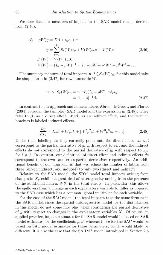
38 Introduction to Spatial Econometrics
We note that our measures of impact for the SAR model can be derivedfrom (2.46).
(In − ρW )y = Xβ + ιnα+ ε
y =k∑r=1
Sr(W )xr + V (W )ιnα+ V (W )ε (2.46)
Sr(W ) = V (W )InβrV (W ) = (In − ρW )−1 = In + ρW + ρ2W 2 + ρ3W 3 + . . .
The summary measure of total impacts, n−1ι′nSr(W )ιn, for this model takethe simple form in (2.47) for row-stochastic W .
n−1ι′nSr(W )ιn = n−1ι′n(In − ρW )−1βrιn
= (1 − ρ)−1βr (2.47)
In contrast to our approach and nomenclature, Abreu, de Groot, and Florax(2004) consider the (simpler) SAR model and the expression in (2.48). Theyrefer to βr as a direct effect, Wρβr as an indirect effect, and the term inbrackets is labeled induced effects.
∂y
∂x′r= Inβr +Wρβr + [W 2ρ2βr +W 3ρ3βr + . . .] (2.48)
Under their labeling, as they correctly point out, the direct effects do notcorrespond to the partial derivative of yi with respect to xir , and the indirecteffects do not correspond to the partial derivative of yi with respect to xjrfor i �= j. In contrast, our definitions of direct effect and indirect effects docorrespond to the own- and cross-partial derivatives respectively. An addi-tional benefit of our approach is that we reduce the number of labels fromthree (direct, indirect, and induced) to only two (direct and indirect).
Relative to the SAR model, the SDM model total impacts arising fromchanges in Xr exhibit a great deal of heterogeneity arising from the presenceof the additional matrix Wθr in the total effects. In particular, this allowsthe spillovers from a change in each explanatory variable to differ as opposedto the SAR case which has a common, global multiplier for each variable.
For the case of the SAC model, the total impacts take the same form as inthe SAR model, since the spatial autoregressive model for the disturbancesin this model do not come into play when considering the partial derivativeof y with respect to changes in the explanatory variables X . Of course, inapplied practice, impact estimates for the SAR model would be based on SARmodel estimates for the coefficients ρ, β, whereas those for the SAC would bebased on SAC model estimates for these parameters, which would likely bedifferent. It is also the case that the SARMA model introduced in Section 2.6
© 2009 by Taylor & Francis Group, LLC
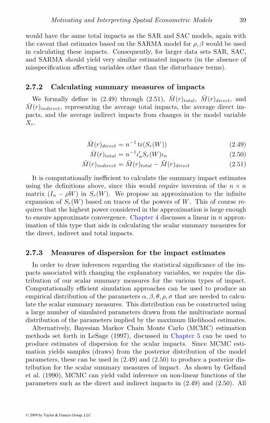
Motivating and Interpreting Spatial Econometric Models 39
would have the same total impacts as the SAR and SAC models, again withthe caveat that estimates based on the SARMA model for ρ, β would be usedin calculating these impacts. Consequently, for larger data sets SAR, SAC,and SARMA should yield very similar estimated impacts (in the absence ofmisspecification affecting variables other than the disturbance terms).
2.7.2 Calculating summary measures of impacts
We formally define in (2.49) through (2.51), M(r)total, M(r)direct, andM(r)indirect, representing the average total impacts, the average direct im-pacts, and the average indirect impacts from changes in the model variableXr.
M(r)direct = n−1 tr(Sr(W )) (2.49)M(r)total = n−1ι′nSr(W )ιn (2.50)
M(r)indirect = M(r)total − M(r)direct (2.51)
It is computationally inefficient to calculate the summary impact estimatesusing the definitions above, since this would require inversion of the n × nmatrix (In − ρW ) in Sr(W ). We propose an approximation to the infiniteexpansion of Sr(W ) based on traces of the powers of W . This of course re-quires that the highest power considered in the approximation is large enoughto ensure approximate convergence. Chapter 4 discusses a linear in n approx-imation of this type that aids in calculating the scalar summary measures forthe direct, indirect and total impacts.
2.7.3 Measures of dispersion for the impact estimates
In order to draw inferences regarding the statistical significance of the im-pacts associated with changing the explanatory variables, we require the dis-tribution of our scalar summary measures for the various types of impact.Computationally efficient simulation approaches can be used to produce anempirical distribution of the parameters α, β, θ, ρ, σ that are needed to calcu-late the scalar summary measures. This distribution can be constructed usinga large number of simulated parameters drawn from the multivariate normaldistribution of the parameters implied by the maximum likelihood estimates.
Alternatively, Bayesian Markov Chain Monte Carlo (MCMC) estimationmethods set forth in LeSage (1997), discussed in Chapter 5 can be used toproduce estimates of dispersion for the scalar impacts. Since MCMC esti-mation yields samples (draws) from the posterior distribution of the modelparameters, these can be used in (2.49) and (2.50) to produce a posterior dis-tribution for the scalar summary measures of impact. As shown by Gelfandet al. (1990), MCMC can yield valid inference on non-linear functions of theparameters such as the direct and indirect impacts in (2.49) and (2.50). All
© 2009 by Taylor & Francis Group, LLC
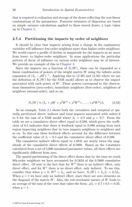
40 Introduction to Spatial Econometrics
that is required is evaluation and storage of the draws reflecting the non-linearcombinations of the parameters. Posterior estimates of dispersion are basedon simple variance calculations applied to these stored draws, a topic takenup in Chapter 5.
2.7.4 Partitioning the impacts by order of neighbors
It should be clear that impacts arising from a change in the explanatoryvariables will influence low-order neighbors more than higher-order neighbors.We would expect a profile of decline in magnitude for the impacts as we movefrom lower- to higher-order neighbors. In some applications the particularpattern of decay of influence on various order neighbors may be of interest.We provide an example of this in Chapter 3.
Since the impacts are a function of Sr(W ), these can be expanded as alinear combination of powers of the weight matrix W using the infinite seriesexpansion of (In − ρW )−1. Applying this to (2.49) and (2.50) where we usethe definition of Sr(W ) for the SAR model allows us to observe the impactassociated with each power of W . These powers correspond to the observa-tions themselves (zero-order), immediate neighbors (first-order), neighbors ofneighbors (second-order), and so on.
Sr(W ) ≈ (In + ρW + ρ2W 2 + ρ3W 3+, . . . ,+ρqW q)βr (2.52)
As an example, Table 2.1 shows both the cumulative and marginal or spa-tially partitioned direct, indirect and total impacts associated with orders 0to 9 for the case of a SAR model where βr = 0.5 and ρ = 0.7. From thetable we see a cumulative direct effect equal to 0.586, which given the coeffi-cient of 0.5 indicates that there is feedback equal to 0.086 arising from eachregion impacting neighbors that in turn impacts neighbors to neighbors andso on. In this case these feedback effects account for the difference betweenthe coefficient value of βr = 0.5 and the cumulative direct effect of 0.586.
The cumulative indirect effects equal to 1.0841 are nearly twice the mag-nitude of the cumulative direct effects of 0.5860. Based on the t-statisticscalculated from a set of 5,000 simulated parameter values, all three effects aresignificantly different from zero.
The spatial partitioning of the direct effect shows that by the time we reach9th-order neighbors we have accounted for 0.5834 of the 0.5860 cumulativedirect effect. Of note is the fact that for W 0 there is no indirect effect, onlydirect effect, and for W 1 there is no direct effect, only indirect. To see this,consider that when q = 0, W 0 = In, and we have: Sr(W ) = Inβr = 0.5In.When q = 1 we have only an indirect effect, since there are zero elements onthe diagonal of the matrix W . Also, the row-stochastic nature of W leads toan average of the sum of the rows that takes the form: ρβr = 0.7×0.5 = 0.35,when q = 1.
© 2009 by Taylor & Francis Group, LLC
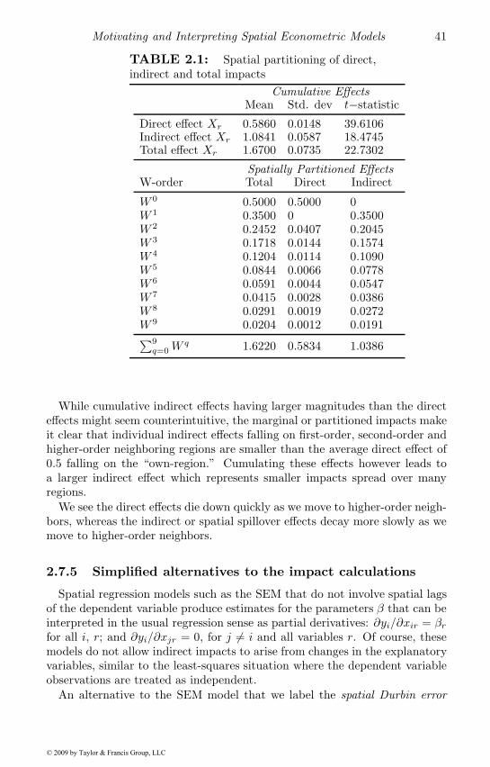
Motivating and Interpreting Spatial Econometric Models 41
TABLE 2.1: Spatial partitioning of direct,indirect and total impacts
Cumulative EffectsMean Std. dev t−statistic
Direct effect Xr 0.5860 0.0148 39.6106Indirect effect Xr 1.0841 0.0587 18.4745Total effect Xr 1.6700 0.0735 22.7302
Spatially Partitioned EffectsW-order Total Direct Indirect
W 0 0.5000 0.5000 0W 1 0.3500 0 0.3500W 2 0.2452 0.0407 0.2045W 3 0.1718 0.0144 0.1574W 4 0.1204 0.0114 0.1090W 5 0.0844 0.0066 0.0778W 6 0.0591 0.0044 0.0547W 7 0.0415 0.0028 0.0386W 8 0.0291 0.0019 0.0272W 9 0.0204 0.0012 0.0191∑9q=0W
q 1.6220 0.5834 1.0386
While cumulative indirect effects having larger magnitudes than the directeffects might seem counterintuitive, the marginal or partitioned impacts makeit clear that individual indirect effects falling on first-order, second-order andhigher-order neighboring regions are smaller than the average direct effect of0.5 falling on the “own-region.” Cumulating these effects however leads toa larger indirect effect which represents smaller impacts spread over manyregions.
We see the direct effects die down quickly as we move to higher-order neigh-bors, whereas the indirect or spatial spillover effects decay more slowly as wemove to higher-order neighbors.
2.7.5 Simplified alternatives to the impact calculations
Spatial regression models such as the SEM that do not involve spatial lagsof the dependent variable produce estimates for the parameters β that can beinterpreted in the usual regression sense as partial derivatives: ∂yi/∂xir = βrfor all i, r; and ∂yi/∂xjr = 0, for j �= i and all variables r. Of course, thesemodels do not allow indirect impacts to arise from changes in the explanatoryvariables, similar to the least-squares situation where the dependent variableobservations are treated as independent.
An alternative to the SEM model that we label the spatial Durbin error
© 2009 by Taylor & Francis Group, LLC
42 Introduction to Spatial Econometrics
model (SDEM) includes a spatial lag of the explanatory variables WX , aswell as spatially dependent disturbances. This model, which augments theSEM model with a spatial lag of the explanatory variables is shown in (2.53),with the model DGP in (2.54).
y = Xβ +WXγ + ιnα+ u (2.53)u = R−1ε
y = Xβ +WXγ + ιnα+R−1ε (2.54)R = In − ρW
E(y) =k∑r=1
Sr(W )xr + ιnα (2.55)
Sr(W ) = (Inβr +Wγr)
The SDEM model does not allow for a separate lagged dependent variableeffect, but does allow for spatially dependent errors and spatial lags of theexplanatory variables. Relative to the more general SDM, it simplifies in-terpretation of the impacts, since the direct impacts are represented by themodel parameters β and indirect impacts correspond to γ. This also allowsus to use measures of dispersion such as the standard deviation or t-statisticfor these regression parameters as a basis for inference regarding significanceof the direct and indirect impacts.
The version of the SDEM in (2.53) uses the same spatial weight matrixfor the errors and the spatially lagged explanatory variables, but this couldbe generalized to allow for different weights and not affect the simplicity ofinterpreting the direct and indirect impacts as corresponding to the modelparameters.
The SDEM replaces the global multiplier found in the SDM with localmultipliers that simplify interpretation of the model estimates. However, wenote that the SDEM could result in underestimation of higher-order (global)indirect impacts. The SDEM does not nest the SDM and vice versa. However,one can devise an extended SDM that nests the SDEM.
2.8 Chapter summary
We provided numerous motivations for why spatial regression relationshipsmight arise that include spatial lags of the dependent variable vector. Modelscontaining spatially lagged dependent variables have been used most oftenin situations where there is an intuitive or theoretical motivation that y willdepend on neighboring values of y. For example, the hedonic housing price
© 2009 by Taylor & Francis Group, LLC

Motivating and Interpreting Spatial Econometric Models 43
literature where it is generally thought that home prices depend on prices ofrecently sold neighboring homes. This is because appraisers/real estate agentspresumably use information on recently sold homes to determine the askingprice. Another example is competition between local governments, where itseems intuitive that local governments can react to actions taken by nearbylocal governments.
There may be a wider role for these models than previously thought sincewe were able to provide three motivations based on: omitted variables, space-time dependence and model uncertainty that resulted in models involvingspatial lags of the dependent variable.
This type of development has wide-ranging implications for the interfaceof economic theory and spatial econometrics. It suggests that spatial econo-metric models may be applicable in many situations where they have notpreviously been employed.
© 2009 by Taylor & Francis Group, LLC
Chapter 3
Maximum Likelihood Estimation
As shown in Chapter 2, estimation of spatial models via least squares can leadto inconsistent estimates of the regression parameters for models with spatiallylagged dependent variables, inconsistent estimation of the spatial parameters,and inconsistent estimation of standard errors. In contrast, maximum likeli-hood is consistent for these models (Lee, 2004). Consequently, this chapterfocuses on maximum likelihood estimation of spatial regression models. His-torically, much of the spatial econometrics literature has focused on waysto avoid maximum likelihood estimation because of perceived computationaldifficulties. There have been a great many improvements in computationalmethods for maximum likelihood estimation of spatial regression models sincethe time of Anselin’s 1988 text. These improvements allow models involvingsamples containing more than 60,000 US Census tract observations to be es-timated in only a few seconds on desktop and laptop computers.
Section 3.1 addresses maximum likelihood estimation for the SAR, SDM,SEM, and other models. Section 3.1 provides a number of techniques thatgreatly reduce previous computational difficulties that arose in estimation ofthese models. Section 3.2 turns attention to maximum likelihood estimation ofvariance-covariance estimates of dispersion for the model parameters requiredfor inference. We provide a new approach that can be used to reduce thecomputational tasks needed to construct maximum likelihood estimates ofdispersion needed for inference.
As already motivated, omitted variables are a likely problem in applied workwith regional economic data, and Section 3.3 further explores the empiricalimpact of spatial dependence on omitted variables bias in spatial regressionmodels. We present theoretical expressions for the bias along with statisti-cal tests and model specifications that mitigate problems posed by omittedvariables that are correlated with included explanatory variables.
The chapter concludes with an application in Section 3.4 that illustratesmany of the issues discussed in the chapter. We rely on a simple modelcontaining a single explanatory variable used to explain factor productivitydifferences among European Union regions.
45© 2009 by Taylor & Francis Group, LLC
46 Introduction to Spatial Econometrics
3.1 Model estimation
We address maximum likelihood estimation for the family of spatial regres-sion models including SAR, SDM, SEM and SAC, which were introduced inSection 2.6. The spatial Durbin model (SDM) provides a general startingpoint for discussion of spatial regression model estimation since this modelsubsumes the spatial error model (SEM) and the spatial autoregressive model(SAR).
In Section 3.1.1 we discuss maximum likelihood estimation of the SAR andSDM models whose likelihood functions coincide. In Section 3.1.2 we turnattention to the SEM model likelihood function and estimation procedure,and models involving multiple weight matrices are discussed in Section 3.1.3.
3.1.1 SAR and SDM model estimation
The SDM model is shown in (3.1) along with its associated data generatingprocess in (3.2),
y = ρWy + αιn +Xβ +WXθ+ ε (3.1)y = (In − ρW )−1 (αιn +Xβ +WXθ + ε) (3.2)ε ∼ N(0, σ2In)
where 0 represents an n× 1 vector of zeros and ιn represents an n× 1 vectorof ones associated with the constant term parameter α. This model can bewritten as a SAR model by defining: Z =
[ιn X WX
]and δ =
[α β θ
]′,leading to (3.3). This means that the likelihood function for SAR and SDMmodels can be written in the same form where: Z =
[ιn X
]for the SAR
model and Z =[ιn X WX
]for the SDM model.
y = ρWy + Zδ + ε (3.3)y = (In − ρW )−1Zδ + (In − ρW )−1ε (3.4)ε ∼ N(0, σ2In)
From the model statement (3.3), if the true value of the parameter ρ wasknown to be say ρ∗, we could rearrange the model statement in (3.3) as shownin (3.5).
y − ρ∗Wy = Zδ + ε (3.5)
This suggests an estimate for δ of δ = (Z ′Z)−1Z ′(In − ρ∗W )y. In thiscase we could also find an estimate for the noise variance parameter σ2 =n−1e(ρ∗)′e(ρ∗), where e(ρ∗) = y − ρ∗Wy − Zδ.
© 2009 by Taylor & Francis Group, LLC
Maximum Likelihood Estimation 47
These ideas motivate that we can concentrate the full (log) likelihood withrespect to the parameters β, σ2 and reduce maximum likelihood to a univariateoptimization problem in the parameter ρ.
Maximizing the full log-likelihood for the case of the SAR model wouldinvolve setting the first derivatives with respect to the parameters β, σ2 andρ equal to zero and simultaneously solving these first-order conditions for allparameters.
In contrast, equivalent maximum likelihood estimates could be found usingthe log-likelihood function concentrated with respect to the parameters β andσ2. This involves substituting closed-form solutions from the first order con-ditions for the parameters β and σ2 to yield a log-likelihood that is said tobe concentrated with respect to these parameters. We label these expressionsβ(ρ), σ2(ρ), and note that they depend on sample data plus the unknown pa-rameter ρ. In the case of the SAR model, this leaves us with a concentratedlog-likelihood that depends only on the single scalar parameter ρ. Optimizingthe concentrated log-likelihood function with respect to ρ, to find the maxi-mum likelihood estimate ρ allows us to use this estimate in the closed-formexpressions for β(ρ) and σ2(ρ) to produce maximum likelihood estimates forthese parameters.
Working with the concentrated log-likelihood yields exactly the same max-imum likelihood estimates β, σ, and ρ as would arise from maximizing thefull log-likelihood (Davidson and MacKinnon, 1993, p. 267-269). The mo-tivation for optimizing the concentrated log-likelihood is that this simplifiesthe optimization problem by reducing a multivariate optimization problemto a univariate problem. Another advantage of using the concentrated log-likelihood is that simple adjustments to output from the optimization problem(that we describe later) can be used to produce a computationally efficientvariance-covariance matrix that we use for inference regarding the parameters.These inferences are identical to those that would be obtained from solvingthe more cumbersome optimization problem involving the full log-likelihood.
The log-likelihood function for the SDM (and SAR) models takes the formin (3.6) (Anselin, 1988, p. 63), where ω is the n × 1 vector of eigenvalues ofthe matrix W .
lnL = −(n/2) ln(πσ2) + ln |In − ρW | − e′e2σ2
(3.6)
e = y − ρWy − Zδ
ρ ∈ (min(ω)−1,max(ω)−1)
If ω contains only real eigenvalues, a positive definite variance-covariance ma-trix is ensured by the condition: ρ ∈ (min(ω)−1,max(ω)−1), as shown in Ord(1975). The matrix W can always be constructed to have a maximum eigen-value of 1. For example, scaling the weight matrix by its maximum eigenvalueas noted by Barry and Pace (1999); Kelejian and Prucha (2007). In this case,
© 2009 by Taylor & Francis Group, LLC
48 Introduction to Spatial Econometrics
the interval for ρ becomes (min(ω)−1, 1) and a subset of this widely employedin practice is ρ ∈ [0, 1). We provide more details regarding the admissiblevalues for ρ in Chapter 4. The admissible values can become more compli-cated for non-symmetric weight matrices W since these may have complexeigenvalues.
As noted, the log-likelihood can be concentrated with respect to the coef-ficient vector δ and the noise variance parameter σ2. Pace and Barry (1997)suggested a convenient approach to concentrating out the parameters δ andσ2, shown in (3.7). The term κ is a constant that does not depend on theparameter ρ, and |In − ρW | is the determinant of this n × n matrix. Weuse the notation e(ρ) to indicate that this vector depends on values taken bythe parameter ρ, as does the scalar concentrated log-likelihood function valuelnL(ρ).
lnL(ρ) = κ+ ln |In − ρW | − (n/2) ln(S(ρ)) (3.7)S(ρ) = e(ρ)′e(ρ) = e′oeo − 2ρe′oed + ρ2e′dede(ρ) = eo − ρed
eo = y − Zδo
ed = Wy − Zδd
δo = (Z ′Z)−1Z ′yδd = (Z ′Z)−1Z ′Wy
To simplify optimization of the log-likelihood with respect to the scalarparameter ρ, Pace and Barry (1997) proposed evaluating the log-likelihoodusing a q × 1 vector of values for ρ in the interval [ρmin, ρmax], labeled asρ1, . . . , ρq in (3.8).
⎛⎜⎜⎜⎝lnL(ρ1)lnL(ρ2)
...lnL(ρq)
⎞⎟⎟⎟⎠ = κ+
⎛⎜⎜⎜⎝ln |In − ρ1W |ln |In − ρ2W |
...ln |In − ρqW |
⎞⎟⎟⎟⎠− (n/2)
⎛⎜⎜⎜⎝ln(S(ρ1))ln(S(ρ2))
...ln(S(ρq))
⎞⎟⎟⎟⎠ (3.8)
In Chapter 4 we discuss a number of approaches to efficiently calculating theterm ln |In−ρiW | over a vector of values for the parameter ρ. In our discussionhere, we simply assume that these values are available during optimizationof the log-likelihood. Given a sufficiently fine grid of q values for the log-likelihood, interpolation can supply intervening points to any desired accuracy(which follows from the smoothness of the log-likelihood function). Note, thescalar moments e′oeo, e
′deo, and e′ded and the k×1 vectors δo, δd are computed
prior to optimization, and so given a value for ρ, calculating S(ρ) simplyrequires weighting three numbers. Given the optimum value of ρ, this becomesthe maximum likelihood estimate of ρ denoted as ρ. Therefore, it requires verylittle computation to arrive at the vector of concentrated log-likelihood values.
© 2009 by Taylor & Francis Group, LLC
Maximum Likelihood Estimation 49
Given the maximum likelihood estimate ρ, (3.9), (3.10), and (3.11) showthe maximum likelihood estimates for the coefficients δ, the noise varianceparameter σ2, and associated variance-covariance matrix for the disturbances.
δ = δo − ρδd (3.9)σ2 = n−1S(ρ) (3.10)
Ω = σ2 [(In − ρW )′(In − ρW )]−1 (3.11)
Although the vectorized approach works well, Chapter 4 discusses an alterna-tive closed-form solution technique for ρ. However, we prefer to discuss thevectorized approach here due to its simplicity.
The likelihood function combines a transformed sum-of-squared errors termwith the log determinant term acting as a penalty function that prevents themaximum likelihood estimate of ρ from being equal to an estimate based solelyon the minimized (transformed) sum of squared errors, S(ρ). The vectorizedapproach provides the additional advantage of ensuring a global as opposedto a local optimum.
Maximum likelihood estimation could proceed using a variety of univariateoptimization techniques. These could include the vectorized approach justdiscussed based on a fine grid of values of ρ (large q), non-derivative searchmethods such as the Nelder-Mead simplex or bisection search scheme, or byapplying a derivative-based optimization technique (Press et al., 1996). Someform of Newton’s method with numerical derivatives has the advantage ofproviding the optimum as well as the second derivative of the concentrated loglikelihood at the optimum ρ. This numerical estimate of the second derivativein conjunction with other information can be useful in producing a numericalestimate of the variance-covariance matrix for the parameters. We discussthis topic in more detail in Section 3.2.
As shown above, an apparent barrier to implementing these models for largen is the n×n matrix W . If W contains all non-zero elements, it would requireenormous amounts of memory to store this matrix for problems involving largesamples such as the US Census tracts where n > 60, 000. Fortunately, W isusually sparse, meaning it contains a large proportion of zeros. For example,if one relies on contiguous regions or some number m of nearest neighboringregions to form W , the spatial weight matrix will only contain mn non-zerosas opposed to n2 non-zeros for a dense matrix. The proportion of non-zerosbecomes m/n which falls with n. Contiguity weight matrices have an averageof six neighbors per row (for spatially random sets of points on a plane). Asan example, using the 3,111 US counties representing the lower 48 states plusthe district of Columbia, there are 9,678,321 elements in the 3, 111 × 3, 111matrix W , but only 3, 111× 6 = 18, 666 would be non-zero, or 0.1929 percentof the entries. In addition, calculating matrix-vector products such as Wy andWX take much less time for sparse matrices. In both cases, sparse matricesrequire linear in n operations ( O(n)) while a dense W would require quadratic
© 2009 by Taylor & Francis Group, LLC
50 Introduction to Spatial Econometrics
in n operations (O(n2)). As shown in Chapter 4, sparse matrix techniquesgreatly accelerate computation of the log-determinant and other quantities ofinterest.
To summarize, a number of techniques facilitate calculation of maximumlikelihood estimates for the SDM and SAR models. These techniques includeconcentrating the log-likelihood, pre-computing a table of log-determinantsas well as moments such as e′oed, and using sparse W . Taken together, thesetechniques greatly reduce the operation counts as well as computer memoryrequired to solve problems involving large data samples. Chapter 4 providesmore detail about these and other techniques that can aid in calculation ofmaximum likelihood estimates.
3.1.2 SEM model estimation
The model statement for a model containing spatial dependence in thedisturbances that we label SEM is shown in (3.12), with the DGP for thismodel in (3.13), where we define X to be the n × k explanatory variablesmatrix that may or may not include a constant term, and β the associatedk × 1 vector of parameters.
y = Xβ + u (3.12)u = λWu+ ε
y = Xβ + (In − λW )−1ε (3.13)ε ∼ N(0, σ2In)
The full log-likelihood has the form in (3.14).
lnL = −(n/2) ln(πσ2) + ln |In − λW | − e′e2σ2
(3.14)
e = (In − λW )(y −Xβ)
For a given λ, optimization of the log-likelihood function shows (Ord, 1975;Anselin, 1988) that β(λ) = (X(λ)′X(λ))−1X(λ)′y(λ), where X(λ) = (X −λWX), y(λ) = (y − λWy), and σ2(λ) = e(λ)′e(λ)/n where e(λ) = y(λ) −X(λ)β(λ). Therefore, we can concentrate the log-likelihood with respect to βand σ2 to yield the concentrated log-likelihood as a function of λ in (3.15).
lnL(λ) = κ+ ln |In − λW | − (n/2) ln (S(λ)) (3.15)S(λ) = e(λ)′e(λ) (3.16)
Unlike the SAR or SDM case, S(λ) is not a simple quadratic in the spatialparameter. As currently stated in (3.16), evaluating the concentrated log-likelihood for any given value of λ requires manipulation of n × 1 and n ×
© 2009 by Taylor & Francis Group, LLC
Maximum Likelihood Estimation 51
k matrices for each choice of λ. This becomes tedious for large data sets,optimization techniques that require many trial values of λ, and in simulations.However, variables that require O(n) computations can be pre-computed sothat calculating S(λ) during optimization only requires working with momentmatrices of dimension k by k or smaller. These moment matrices involve theindependent and dependent variables as a function of λ.1
AXX(λ) = X ′X − λX ′WX − λX ′W ′X + λ2X ′W ′WX
AXy(λ) = X ′y − λX ′Wy − λX ′W ′y + λ2X ′W ′Wy
Ayy(λ) = y′y − λy′Wy − λy′W ′y + λ2y′W ′Wy
β(λ) = AXX(λ)−1AXy(λ)S(λ) = Ayy(λ) − β(λ)′AXX(λ)β(λ)
With these moments and a pre-computed grid of log-determinants (coupledwith an interpolation routine) updating the concentrated log-likelihood in(3.15) for a new value of λ is almost instantaneous. Applying a univariateoptimization technique such as Newton’s method to (3.15) to find λ and sub-stituting this into σ2(λ), β(λ) and Ω(λ) leads to the maximum likelihoodestimates (3.17) to (3.19).
β = β(λ) (3.17)
σ2 = n−1S(λ) (3.18)
Ω = σ2[(In − λW )′(In − λW )
]−1
(3.19)
As noted in Section 3.1.1, applying Newton’s method with numerical deriva-tives to find the optimum produces a numerical estimate of the second deriva-tive of the concentrated log-likelihood at the optimum λ. This numericalestimate of the second derivative can be used in conjunction with other infor-mation to produce a variance-covariance matrix estimate.
Note, the SDM model nests the SEM model as a special case. To see this,consider the alternative statement of the SEM model in (3.20). To avoidcollinearity problems for row-stochastic W , we assume the matrix X does notcontain a constant term and specify this separately. This is necessary to avoidcreating a column vector Wιn = ιn in WX that would duplicate the interceptterm.
1Use of moment matrices requires that we avoid sets of explanatory variables that are poorlyscaled or ill-conditioned. In practice, this may not act as a tremendous constraint since evennumerically robust computational techniques can be strained by ill-conditioned data sets.In addition, poorly scaled sets of explanatory variables often lead to difficult-to-interpretparameter estimates.
© 2009 by Taylor & Francis Group, LLC
52 Introduction to Spatial Econometrics
y = αιn +Xβ + (In − λW )−1ε
(In − λW )y = α(In − λW )ιn + (In − λW )Xβ + ε
y = λWy + α(In − λW )ιn +Xβ +WX(−βλ) + ε (3.20)
The model in (3.20) represents an SDM model where the parameter on thespatial lag of the explanatory variables (WX) has been restricted to equal−βλ. Estimating the more general SDM model ( y = λWy+Xβ+WXθ+ ε)and testing the restriction θ = −βλ could lead to rejection of the SEM relativeto the SDM.
3.1.3 Estimates for models with two weight matrices
The spatial literature contains a number of models involving two or moreweight matrices. Using multiple weight matrices provides a straightforwardgeneralization of the SAR, SDM, and SEM models. For example, Lacombe(2004) uses a two weight matrix SAR model similar to the SDM model shownin (3.21).
y = ρ1W1y + ρ2W2y +Xβ +W1Xγ +W2Xθ + ε (3.21)ε ∼ N(0, σ2In)
The weight matrix W1 was used to capture the effect of neighboring countieswithin the state, and W2 captures the effect of neighboring counties in thebordering state. Lacombe (2004) analyzed policies that varied across states,making this model attractive. For a sample of counties that lie on state bor-ders, spatial dependence extends to both counties within the state as wellas those across the border in the neighboring state. This SDM variant ofLacombe’s model allows for separate influences of the explanatory variablesmatrix X arising from neighbors within the state versus those in the neigh-boring state.
The only departure from our discussion of maximum likelihood estimationfor this variant of the SDM model involves a bivariate optimization problemover the range of feasible values for ρ1, ρ2. Maximizing the (concentrated forβ, γ, θ, σ2) log-likelihood for this variant of the SDM model requires calcu-lating the log-determinant term: ln |In − ρ1W1 − ρ2W2| over a bivariate gridof values for both ρ1, ρ2 in the feasible range. These scalar values associatedwith the bivariate grid would be stored in a matrix rather than a vector.Optimization of the concentrated log-likelihood function over the parametersρ1, ρ2 could repeatedly access this matrix at a very small computational cost.
As another example of specifications involving two weight matrices, theSAC model contains spatial dependence in both the dependent variable anddisturbances as shown in (3.22) along with its associated data generating
© 2009 by Taylor & Francis Group, LLC
Maximum Likelihood Estimation 53
process in (3.23). Unlike the Lacombe model, it is possible to implement thismodel using the same matrix W = W1 = W2, but we will have more to sayabout this later.
y = ρW1y +Xβ + u
u = λW2u+ ε (3.22)y = (In − ρW1)−1Xβ + (In − ρW1)−1(In − λW2)−1ε (3.23)ε ∼ N(0, σ2In)
The matrices W1,W2 can be the same or distinct. Obviously, if the parameterρ = 0, this model collapses to the SEM model, and λ = 0 yields the SARmodel. Normally, the SAC does not contain a separate WX term, so theSAC does not usually nest the SDM. However, one can write an extendedSDM that nests the SAC, specifically:
y = ρWy +Xβ +WXθ + u
u = λWu+ ε
The log-likelihood for the SAC model is shown in (3.24) along with defini-tions.
lnL = −(n/2) ln(πσ2) + ln |A| + ln |B| − e′e2σ2
(3.24)
e = B(Ay −Xβ)A = In − ρW1
B = In − λW2
The log-likelihood in (3.24) for the SAC model can also be concentratedwith respect to the parameters β, σ2. Maximizing this likelihood requirescomputing two log-determinants for the case where W1 �= W2, and solving abivariate optimization problem in the two parameters ρ and λ.
Anselin (1988) raised questions about identification of the SAC model inthe case of identical matrices W , but Kelejian and Prucha (2007) providean argument that the model is identified for this case. Their argument foridentification requires that Xβ in the DGP makes a material contributiontowards explaining variation in the dependent variable y (β �= 0). To see theimportance of this, consider (3.25), and note that in the case where β = 0, alabel switching problem exists since AB = BA when A and B are functionsof the same weight matrix W . Therefore, the parameters ρ and λ are notidentified.
y = (In − ρW )−1Xβ + (In − ρW )−1(In − λW )−1ε (3.25)
© 2009 by Taylor & Francis Group, LLC
54 Introduction to Spatial Econometrics
Although, β �= 0 will in principle identify the model, as the noise varianceof the disturbances rises, the relative importance of β diminishes. This isshown in (3.26) where the variables are all scaled by σ. This suggests thatin low signal-to-noise problems (low variation in the predicted values relativeto the noise variance), estimates may show symptoms of this near lack ofidentification.
σ−1y = A−1X(σ−1β) + A−1B−1σ−1ε (3.26)
There is also the SARMA model shown in (3.27), with the correspondingDGP in (3.28).
y = ρW1y +Xβ + u
u = (In − θW2)ε (3.27)y = (In − ρW1)−1Xβ + (In − ρW1)−1(In − θW2)ε (3.28)
Minor changes would be required to the log-likelihood function for thismodel as shown in (3.29), where we have replaced the definition B = (In −λW2) from the SAC model with B = (In − θW2)−1.
lnL = κ+ ln |A| + ln |B| − e′e2σ2
(3.29)
e = B(Ay −Xβ)A = In − ρW1
B = (In − θW2)−1
Finally, many other models involving multiple weight matrices or combina-tions of powers of weight matrices have been proposed in the literature such ashigher-order spatial AR, MA, and ARMA models (Huang and Anh, 1992). InChapter 4 we discuss approaches for calculating the determinants that arisein such models.
3.2 Estimates of dispersion for the parameters
So far, the estimation procedures set forth can be used to produce estimatesfor the spatial dependence parameters ρ and λ using univariate or bivariatemaximization of the log-likelihood function concentrated with respect to βand σ2. Maximum likelihood estimates for the parameters β and σ2 can berecovered using the maximum likelihood estimates for the dependence param-eters ρ and λ.
© 2009 by Taylor & Francis Group, LLC
Maximum Likelihood Estimation 55
For many purposes, a need exists to conduct inference. Maximum likeli-hood inference often proceeds using likelihood ratio (LR), Lagrange multiplier(LM), or Wald (W) tests. Asymptotically, these should all yield similar re-sults, although these can differ for finite samples. Often, the choice of onemethod over the other comes down to computational convenience and otherpreferences.
Due to the ability to rapidly compute likelihoods, Pace and Barry (1997)propose likelihood ratio tests for hypotheses such as the deletion of a singleexplanatory variable. To put these likelihood ratio tests in a form similar to t-tests, Pace and LeSage (2003a) discuss use of signed root deviance statistics.2
The signed root deviance applies the sign of the coefficient estimates β tothe square root of the deviance statistic (Chen and Jennrich, 1996). Thesestatistics behave similar to t -ratios when the sample is large, and can be usedin lieu of t -statistics for hypothesis testing.
Wald inference uses the Hessian (numerical or analytic) or the related in-formation matrix to provide a variance-covariance matrix for the estimatedparameters, and thus the familiar t-test. In this case, the Hessian is justthe matrix of second-derivatives of the log-likelihood with respect to the pa-rameters. Approaches using either the Hessian (Anselin, 1988, p. 76) or theinformation matrix (Ord, 1975; Smirnov, 2005) have appeared in the spatialeconometrics literature.
An implementation issue is constructing the Hessian or information matrix.We will use the SAR model: y = ρWy+Xβ+ε for simplicity in our discussion.Straightforward evaluation of the analytical Hessian or information matrixinvolves computing a trace term which contains the dense n×n matrix inverse(In − ρW )−1. Chapter 4 provides means of rapidly approximating elementsthat arise in the Hessian or information matrix. In the following discussionwe focus on the Hessian.
Given the ability to rapidly evaluate the log-likelihood function, a purelynumerical approach might seem feasible for calculating an estimate of theHessian. There are some drawbacks to implementing this approach in soft-ware for general use. First, practitioners often work with poorly scaled sampledata, which makes numerical perturbations used to approximate the deriva-tives comprising the Hessian difficult. A second point is that univariate op-timization takes place using the likelihood concentrated with respect to theparameters β and σ2, so a numerical approximation to the full Hessian doesnot arise naturally, as in typical maximum likelihood estimation procedures.This means that computational time must be spent after estimation of theparameters to produce a separate numerical estimate of the full Hessian.
In Section 3.2.1 we discuss ways of marrying the analytic Hessian and nu-merical Hessian results to take advantage of the strengths of each approach.
2Deviance is minus twice the log of the likelihood ratio for models fitted by maximumlikelihood. The ratio used in these calculations is one involving the likelihood for the modelexcluding each variable versus that for the model containing all variables.
© 2009 by Taylor & Francis Group, LLC
56 Introduction to Spatial Econometrics
Namely, most of the analytic Hessian elements do not require much time tocompute and have less sensitivity to scaling issues. A numerical approach,however, takes less time and performs well for the single difficult element inthe analytic Hessian.
In Chapter 5 Bayesian Markov Chain Monte Carlo (MCMC) estimationmethods for spatial regression models are explained, and these can be usedto produce estimates of dispersion based on the sample of draws carried outby this sampling-based approach to estimation. Following standard Bayesianregression theory, use of a non-informative prior in these models should resultin posterior estimates and inferences that are identical to those from maximumlikelihood. Therefore, these estimates of parameter dispersion also provide avalid, but unorthodox, means of conducting maximum likelihood inference.
Also, for large n it often becomes feasible to provide bounded inference. Forexample, Pace and LeSage (2003a) introduce a lower bound on the likelihoodratio test that allows conservative maximum likelihood inference while avoid-ing the computationally demanding task of even computing exact maximumlikelihood point estimates. They show that this form of likelihood dominanceinference (Pollack and Wales, 1991) performed almost as well as exact likeli-hood inference on parameters from a SAR model involving 890,091 observa-tions, where the procedure took less than a minute to compute.
An entirely different approach to the problem of inference in spatial regres-sion models is to rely on an estimation method that is not likelihood based.Examples include the instrumental variable approach of Anselin (1988, p. 81-90), the instrumental variables/generalized moments estimator from Kelejianand Prucha (1998, 1999) or the maximum entropy of Marsh and Mittelham-mer (2004). Much of the motivation for using these methods comes from theperceived difficulties of computing estimates from likelihood-based methods,a problem that has been largely resolved. A feature of likelihood-based meth-ods is that the determinant term ensures that resulting dependence parameterestimates are in the interval defined by maximum and minimum eigenvaluesof the weight matrix. Some of the alternative estimation methods that avoidusing the log-determinant can fail to yield dependence parameter estimates inthis interval. In addition, these methods can be sensitive in non-obvious waysto various implementation issues such as the interaction between the choiceof instruments and the specification of the model. For these reasons, we focuson likelihood-based techniques.
3.2.1 A mixed analytical-numerical Hessian calculation
For the case of the SAR model, the Hessian we will work with is organizedas in (3.30), which we label H . For the case of the SEM model, we wouldreplace the parameter ρ with λ. Of course, some of the derivative expressionschange as well.
© 2009 by Taylor & Francis Group, LLC
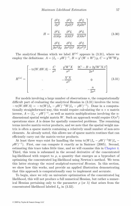
Maximum Likelihood Estimation 57
H =
⎡⎢⎢⎢⎢⎢⎢⎢⎢⎢⎢⎣
∂2L
∂ρ2
∂2L
∂ρ∂β′∂2L
∂ρ∂σ2
∂2L
∂β∂ρ
∂2L
∂β∂β′∂2L
∂β∂σ2
∂2L
∂σ2∂ρ
∂2L
∂σ2∂β′∂2L
∂(σ2)2
⎤⎥⎥⎥⎥⎥⎥⎥⎥⎥⎥⎦(3.30)
The analytical Hessian which we label H(a) appears in (3.31), where weemploy the definitions: A = (In − ρW )−1, B = y′ (W +W ′) y, C = y′W ′Wy.
H(a) =
⎡⎢⎢⎢⎢⎢⎢⎢⎢⎣
− tr(WAWA) − C
σ2−y
′W ′Xσ2
2C −B + 2y′W ′Xβ2σ4
· −X′Xσ2
0
· · − n
2σ4
⎤⎥⎥⎥⎥⎥⎥⎥⎥⎦(3.31)
For models involving a large number of observations n, the computationallydifficult part of evaluating the analytical Hessian in (3.31) involves the term:− tr(WAWA) = − tr(W (In − ρW )−1W (In − ρW )−1). Done in a computa-tionally straightforward way, this would require calculating the n× n matrixinverse, A = (In − ρW )−1, as well as matrix multiplications involving the n-dimensional spatial weight matrix W . Such an approach would require O(n3)operations since A is dense for spatially connected problems. The remainingterms involve matrix-vector products, and we note that the spatial weight ma-trix is often a sparse matrix containing a relatively small number of non-zeroelements. As already noted, this allows use of sparse matrix routines that canefficiently carry out the matrix-vector products.
At least three ways exist for handling the term tr(W (In − ρW )−1W (In −ρW )−1). First, one can compute it exactly as in Smirnov (2005). Second,estimating this trace takes little time, and we will examine this in Chapter 4.Third, this term is subsumed in the second derivative of the concentratedlog-likelihood with respect to ρ, a quantity that emerges as a byproduct ofoptimizing the concentrated log-likelihood using Newton’s method. We termthis latter strategy the mixed analytical-numerical Hessian. In this section,we show how this works, and provide an applied illustration demonstratingthat this approach is computationally easy to implement and accurate.
To begin, since we rely on univariate optimization of the concentrated loglikelihood, this will not produce a full numerical Hessian, but rather a numer-ical Hessian pertaining only to the parameter ρ (or λ) that arises from theconcentrated likelihood labeled Lp in (3.32).
© 2009 by Taylor & Francis Group, LLC
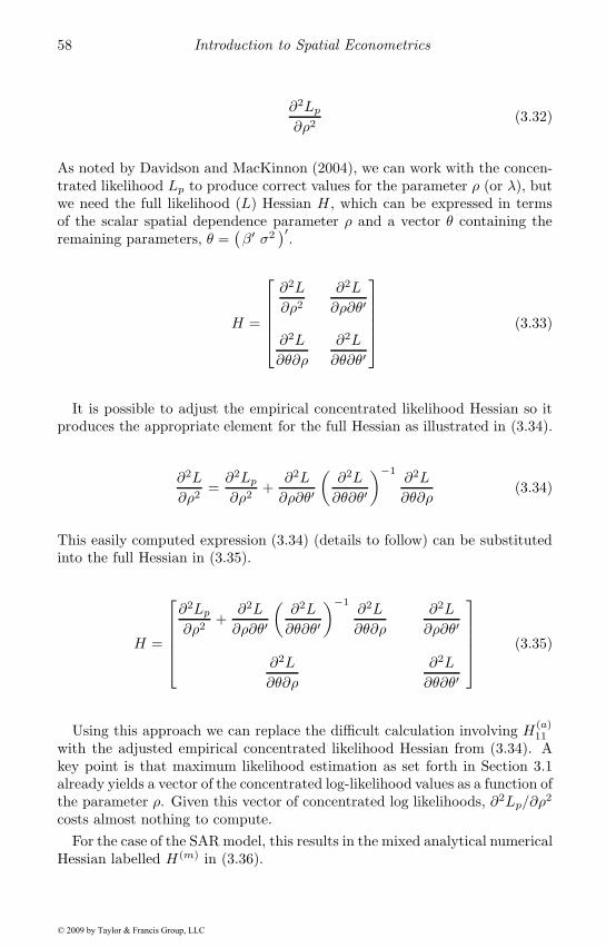
58 Introduction to Spatial Econometrics
∂2Lp∂ρ2
(3.32)
As noted by Davidson and MacKinnon (2004), we can work with the concen-trated likelihood Lp to produce correct values for the parameter ρ (or λ), butwe need the full likelihood (L) Hessian H , which can be expressed in termsof the scalar spatial dependence parameter ρ and a vector θ containing theremaining parameters, θ =
(β′ σ2
)′.
H =
⎡⎢⎢⎢⎢⎣∂2L
∂ρ2
∂2L
∂ρ∂θ′
∂2L
∂θ∂ρ
∂2L
∂θ∂θ′
⎤⎥⎥⎥⎥⎦ (3.33)
It is possible to adjust the empirical concentrated likelihood Hessian so itproduces the appropriate element for the full Hessian as illustrated in (3.34).
∂2L
∂ρ2=∂2Lp∂ρ2
+∂2L
∂ρ∂θ′
(∂2L
∂θ∂θ′
)−1∂2L
∂θ∂ρ(3.34)
This easily computed expression (3.34) (details to follow) can be substitutedinto the full Hessian in (3.35).
H =
⎡⎢⎢⎢⎢⎣∂2Lp∂ρ2
+∂2L
∂ρ∂θ′
(∂2L
∂θ∂θ′
)−1∂2L
∂θ∂ρ
∂2L
∂ρ∂θ′
∂2L
∂θ∂ρ
∂2L
∂θ∂θ′
⎤⎥⎥⎥⎥⎦ (3.35)
Using this approach we can replace the difficult calculation involving H(a)11
with the adjusted empirical concentrated likelihood Hessian from (3.34). Akey point is that maximum likelihood estimation as set forth in Section 3.1already yields a vector of the concentrated log-likelihood values as a function ofthe parameter ρ. Given this vector of concentrated log likelihoods, ∂2Lp/∂ρ
2
costs almost nothing to compute.For the case of the SAR model, this results in the mixed analytical numerical
Hessian labelled H(m) in (3.36).
© 2009 by Taylor & Francis Group, LLC
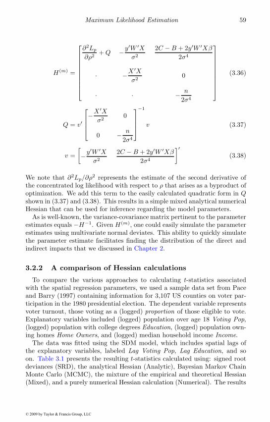
Maximum Likelihood Estimation 59
H(m) =
⎡⎢⎢⎢⎢⎢⎢⎢⎢⎣
∂2Lp∂ρ2
+Q −y′W ′Xσ2
2C −B + 2y′W ′Xβ2σ4
· −X′Xσ2
0
· · − n
2σ4
⎤⎥⎥⎥⎥⎥⎥⎥⎥⎦(3.36)
Q = v′
⎡⎢⎢⎣−X ′Xσ2
0
0 − n
2σ4
⎤⎥⎥⎦−1
v (3.37)
v =[−y
′W ′Xσ2
2C −B + 2y′W ′Xβ2σ4
]′(3.38)
We note that ∂2Lp/∂ρ2 represents the estimate of the second derivative of
the concentrated log likelihood with respect to ρ that arises as a byproduct ofoptimization. We add this term to the easily calculated quadratic form in Qshown in (3.37) and (3.38). This results in a simple mixed analytical numericalHessian that can be used for inference regarding the model parameters.
As is well-known, the variance-covariance matrix pertinent to the parameterestimates equals −H−1. Given H(m), one could easily simulate the parameterestimates using multivariate normal deviates. This ability to quickly simulatethe parameter estimate facilitates finding the distribution of the direct andindirect impacts that we discussed in Chapter 2.
3.2.2 A comparison of Hessian calculations
To compare the various approaches to calculating t-statistics associatedwith the spatial regression parameters, we used a sample data set from Paceand Barry (1997) containing information for 3,107 US counties on voter par-ticipation in the 1980 presidential election. The dependent variable representsvoter turnout, those voting as a (logged) proportion of those eligible to vote.Explanatory variables included (logged) population over age 18 Voting Pop,(logged) population with college degrees Education, (logged) population own-ing homes Home Owners, and (logged) median household income Income.
The data was fitted using the SDM model, which includes spatial lags ofthe explanatory variables, labeled Lag Voting Pop, Lag Education, and soon. Table 3.1 presents the resulting t-statistics calculated using: signed rootdeviances (SRD), the analytical Hessian (Analytic), Bayesian Markov ChainMonte Carlo (MCMC), the mixture of the empirical and theoretical Hessian(Mixed), and a purely numerical Hessian calculation (Numerical). The results
© 2009 by Taylor & Francis Group, LLC
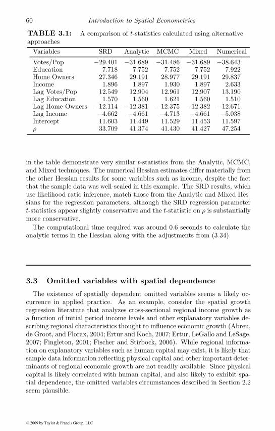
60 Introduction to Spatial Econometrics
TABLE 3.1: A comparison of t-statistics calculated using alternativeapproaches
Variables SRD Analytic MCMC Mixed Numerical
Votes/Pop −29.401 −31.689 −31.486 −31.689 −38.643Education 7.718 7.752 7.752 7.752 7.922Home Owners 27.346 29.191 28.977 29.191 29.837Income 1.896 1.897 1.930 1.897 2.633Lag Votes/Pop 12.549 12.904 12.961 12.907 13.190Lag Education 1.570 1.560 1.621 1.560 1.510Lag Home Owners −12.114 −12.381 −12.375 −12.382 −12.671Lag Income −4.662 −4.661 −4.713 −4.661 −5.038Intercept 11.603 11.449 11.529 11.453 11.597ρ 33.709 41.374 41.430 41.427 47.254
in the table demonstrate very similar t-statistics from the Analytic, MCMC,and Mixed techniques. The numerical Hessian estimates differ materially fromthe other Hessian results for some variables such as income, despite the factthat the sample data was well-scaled in this example. The SRD results, whichuse likelihood ratio inference, match those from the Analytic and Mixed Hes-sians for the regression parameters, although the SRD regression parametert-statistics appear slightly conservative and the t-statistic on ρ is substantiallymore conservative.
The computational time required was around 0.6 seconds to calculate theanalytic terms in the Hessian along with the adjustments from (3.34).
3.3 Omitted variables with spatial dependence
The existence of spatially dependent omitted variables seems a likely oc-currence in applied practice. As an example, consider the spatial growthregression literature that analyzes cross-sectional regional income growth asa function of initial period income levels and other explanatory variables de-scribing regional characteristics thought to influence economic growth (Abreu,de Groot, and Florax, 2004; Ertur and Koch, 2007; Ertur, LeGallo and LeSage,2007; Fingleton, 2001; Fischer and Stirbock, 2006). While regional informa-tion on explanatory variables such as human capital may exist, it is likely thatsample data information reflecting physical capital and other important deter-minants of regional economic growth are not readily available. Since physicalcapital is likely correlated with human capital, and also likely to exhibit spa-tial dependence, the omitted variables circumstances described in Section 2.2seem plausible.
© 2009 by Taylor & Francis Group, LLC

Maximum Likelihood Estimation 61
In Section 3.3.1, we set forth a statistical test comparing ordinary least-squares (OLS) and SEM estimates that can be used to diagnose misspec-ification in general, and the potential existence of omitted variables. Themotivation for this type of comparison is that theory indicates OLS and SEMestimates should be the same if the true DGP is either OLS, SEM, or anyother error model.
A number of authors (Brasington and Hite, 2005; Dubin, 1988; Cressie,1993, p. 25) have suggested that omitted variables affect spatial regressionmethods less than least-squares. In Section 3.3.2 we explore this issue byderiving an expression for OLS omitted variable bias in a univariate versionof the model. We show that spatial dependence in the explanatory variableexacerbates the usual omitted variables bias produced when incorrectly usingOLS to estimate an SEM model in the presence of a spatially dependentomitted variable.
In Section 3.3.3 we explore the conjecture that spatial regression methodssuffer less from omitted variables bias. It is shown that the DGP associatedwith spatially dependent omitted variables matches the SDM DGP. Use ofthis model in the presence of omitted variables shrinks the bias relative toOLS estimates, which provides a strong econometric motivation for use of theSDM model in applied work. Good theoretical motivations exist for the SDMmodel as well (Ertur and Koch, 2007).
3.3.1 A Hausman test for OLS and SEM estimates
As already noted in Section 2.2, OLS estimates for the parameters β will beunbiased if the underlying DGP represents the SEM model, but t-statisticsfrom least-squares are biased. As shown in Section 2.2, specification errorarising from the presence of omitted variables correlated with the explana-tory variable and spatial dependence in the disturbances will lead to a DGPreflecting the SDM model. As shown in Section 3.1.2, the SDM model neststhe SEM model as a special case, providing the intuition for this result.
We explore a formal statistical test for equality of the coefficient estimatesfrom OLS and SEM, since passing this test would be a good indication thatspecification problems (such as omitted variables correlated with the explana-tory variables) were not present in the SEM model.
As motivation for the test, we note that if the true DGP is any error model,in a repeated sampling context the average of the error model parameterestimates for β should be equal. This is true even with omitted variables,provided that these are independent of X . To see this, consider the errormodel DGP in (3.39) where F is some unknown, arbitrary, fixed matrix, and zis an omitted variable that is independent of X . Consider the generalized leastsquares (GLS) estimator in (3.40) based on some arbitrary, fixed variance-covariance matrix G which may bear no relation to a function of F . Forany choice of F and G, even in the presence of z, the expected value of theestimates equals β as shown in (3.41).
© 2009 by Taylor & Francis Group, LLC
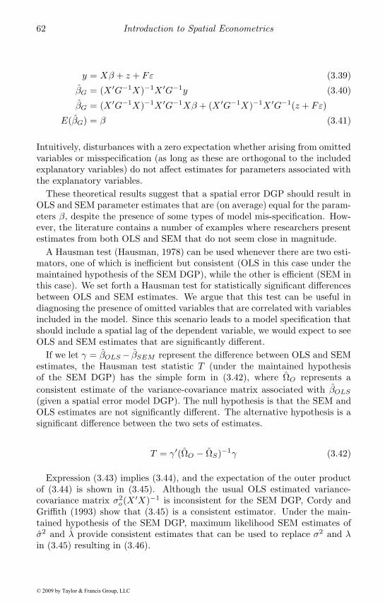
62 Introduction to Spatial Econometrics
y = Xβ + z + Fε (3.39)
βG = (X ′G−1X)−1X ′G−1y (3.40)
βG = (X ′G−1X)−1X ′G−1Xβ + (X ′G−1X)−1X ′G−1(z + Fε)
E(βG) = β (3.41)
Intuitively, disturbances with a zero expectation whether arising from omittedvariables or misspecification (as long as these are orthogonal to the includedexplanatory variables) do not affect estimates for parameters associated withthe explanatory variables.
These theoretical results suggest that a spatial error DGP should result inOLS and SEM parameter estimates that are (on average) equal for the param-eters β, despite the presence of some types of model mis-specification. How-ever, the literature contains a number of examples where researchers presentestimates from both OLS and SEM that do not seem close in magnitude.
A Hausman test (Hausman, 1978) can be used whenever there are two esti-mators, one of which is inefficient but consistent (OLS in this case under themaintained hypothesis of the SEM DGP), while the other is efficient (SEM inthis case). We set forth a Hausman test for statistically significant differencesbetween OLS and SEM estimates. We argue that this test can be useful indiagnosing the presence of omitted variables that are correlated with variablesincluded in the model. Since this scenario leads to a model specification thatshould include a spatial lag of the dependent variable, we would expect to seeOLS and SEM estimates that are significantly different.
If we let γ = βOLS− βSEM represent the difference between OLS and SEMestimates, the Hausman test statistic T (under the maintained hypothesisof the SEM DGP) has the simple form in (3.42), where ΩO represents aconsistent estimate of the variance-covariance matrix associated with βOLS(given a spatial error model DGP). The null hypothesis is that the SEM andOLS estimates are not significantly different. The alternative hypothesis is asignificant difference between the two sets of estimates.
T = γ′(ΩO − ΩS)−1γ (3.42)
Expression (3.43) implies (3.44), and the expectation of the outer productof (3.44) is shown in (3.45). Although the usual OLS estimated variance-covariance matrix σ2
o(X′X)−1 is inconsistent for the SEM DGP, Cordy and
Griffith (1993) show that (3.45) is a consistent estimator. Under the main-tained hypothesis of the SEM DGP, maximum likelihood SEM estimates ofσ2 and λ provide consistent estimates that can be used to replace σ2 and λin (3.45) resulting in (3.46).
© 2009 by Taylor & Francis Group, LLC
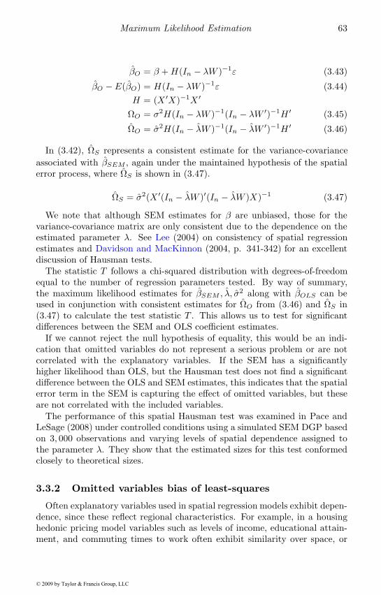
Maximum Likelihood Estimation 63
βO = β +H(In − λW )−1ε (3.43)
βO − E(βO) = H(In − λW )−1ε (3.44)H = (X ′X)−1X ′
ΩO = σ2H(In − λW )−1(In − λW ′)−1H ′ (3.45)
ΩO = σ2H(In − λW )−1(In − λW ′)−1H ′ (3.46)
In (3.42), ΩS represents a consistent estimate for the variance-covarianceassociated with βSEM , again under the maintained hypothesis of the spatialerror process, where ΩS is shown in (3.47).
ΩS = σ2(X ′(In − λW )′(In − λW )X)−1 (3.47)
We note that although SEM estimates for β are unbiased, those for thevariance-covariance matrix are only consistent due to the dependence on theestimated parameter λ. See Lee (2004) on consistency of spatial regressionestimates and Davidson and MacKinnon (2004, p. 341-342) for an excellentdiscussion of Hausman tests.
The statistic T follows a chi-squared distribution with degrees-of-freedomequal to the number of regression parameters tested. By way of summary,the maximum likelihood estimates for βSEM , λ, σ2 along with βOLS can beused in conjunction with consistent estimates for ΩO from (3.46) and ΩS in(3.47) to calculate the test statistic T . This allows us to test for significantdifferences between the SEM and OLS coefficient estimates.
If we cannot reject the null hypothesis of equality, this would be an indi-cation that omitted variables do not represent a serious problem or are notcorrelated with the explanatory variables. If the SEM has a significantlyhigher likelihood than OLS, but the Hausman test does not find a significantdifference between the OLS and SEM estimates, this indicates that the spatialerror term in the SEM is capturing the effect of omitted variables, but theseare not correlated with the included variables.
The performance of this spatial Hausman test was examined in Pace andLeSage (2008) under controlled conditions using a simulated SEM DGP basedon 3, 000 observations and varying levels of spatial dependence assigned tothe parameter λ. They show that the estimated sizes for this test conformedclosely to theoretical sizes.
3.3.2 Omitted variables bias of least-squares
Often explanatory variables used in spatial regression models exhibit depen-dence, since these reflect regional characteristics. For example, in a housinghedonic pricing model variables such as levels of income, educational attain-ment, and commuting times to work often exhibit similarity over space, or
© 2009 by Taylor & Francis Group, LLC
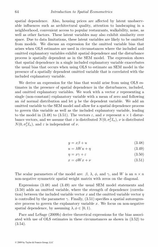
64 Introduction to Spatial Econometrics
spatial dependence. Also, housing prices are affected by latent unobserv-able influences such as architectural quality, attention to landscaping in aneighborhood, convenient access to popular restaurants, walkability, noise, aswell as other factors. These latent variables may also exhibit similarity overspace. Due to data limitations, these latent variables are likely to be omittedfrom models. We discuss an expression for the omitted variable bias thatarises when OLS estimates are used in circumstances where the included andomitted explanatory variables exhibit spatial dependence and the disturbanceprocess is spatially dependent as in the SEM model. The expression showsthat spatial dependence in a single included explanatory variable exacerbatesthe usual bias that occurs when using OLS to estimate an SEM model in thepresence of a spatially dependent omitted variable that is correlated with theincluded explanatory variable.
We derive an expression for the bias that would arise from using OLS es-timates in the presence of spatial dependence in the disturbances, included,and omitted explanatory variables. We work with a vector x representing asingle (non-constant) explanatory variable with a mean of zero and followingan iid normal distribution and let y be the dependent variable. We add anomitted variable to the SEM model and allow for a spatial dependence processto govern this variable as well as the included explanatory variable, leadingto the model in (3.48) to (3.51). The vectors ε, and ν represent n× 1 distur-bance vectors, and we assume that ε is distributed N(0, σ2
εIn), ν is distributedN(0, σ2
νIn), and ε is independent of ν.
y = xβ + u (3.48)u = λWu+ η (3.49)η = xγ + ε (3.50)x = φWx+ ν (3.51)
The scalar parameters of the model are: β, λ, φ, and γ, and W is an n × nnon-negative symmetric spatial weight matrix with zeros on the diagonal.
Expressions (3.48) and (3.49) are the usual SEM model statements and(3.50) adds an omitted variable, where the strength of dependence (correla-tion) between the included variable vector x and the omitted variable vector ηis controlled by the parameter γ. Finally, (3.51) specifies a spatial autoregres-sive process to govern the explanatory variable x. We focus on non-negativespatial dependence, by assuming λ, φ ∈ [0, 1).
Pace and LeSage (2009b) derive theoretical expressions for the bias associ-ated with use of OLS estimates in these circumstances as shown in (3.52) to(3.54).
© 2009 by Taylor & Francis Group, LLC
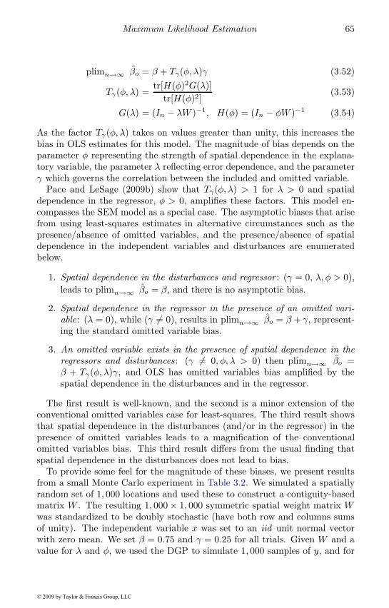
Maximum Likelihood Estimation 65
plimn→∞ βo = β + Tγ(φ, λ)γ (3.52)
Tγ(φ, λ) =tr[H(φ)2G(λ)]
tr[H(φ)2](3.53)
G(λ) = (In − λW )−1, H(φ) = (In − φW )−1 (3.54)
As the factor Tγ(φ, λ) takes on values greater than unity, this increases thebias in OLS estimates for this model. The magnitude of bias depends on theparameter φ representing the strength of spatial dependence in the explana-tory variable, the parameter λ reflecting error dependence, and the parameterγ which governs the correlation between the included and omitted variable.
Pace and LeSage (2009b) show that Tγ(φ, λ) > 1 for λ > 0 and spatialdependence in the regressor, φ > 0, amplifies these factors. This model en-compasses the SEM model as a special case. The asymptotic biases that arisefrom using least-squares estimates in alternative circumstances such as thepresence/absence of omitted variables, and the presence/absence of spatialdependence in the independent variables and disturbances are enumeratedbelow.
1. Spatial dependence in the disturbances and regressor : (γ = 0, λ, φ > 0),leads to plimn→∞ βo = β, and there is no asymptotic bias.
2. Spatial dependence in the regressor in the presence of an omitted vari-able: (λ = 0), while (γ �= 0), results in plimn→∞ βo = β + γ, represent-ing the standard omitted variable bias.
3. An omitted variable exists in the presence of spatial dependence in theregressors and disturbances : (γ �= 0, φ, λ > 0) then plimn→∞ βo =β + Tγ(φ, λ)γ, and OLS has omitted variables bias amplified by thespatial dependence in the disturbances and in the regressor.
The first result is well-known, and the second is a minor extension of theconventional omitted variables case for least-squares. The third result showsthat spatial dependence in the disturbances (and/or in the regressor) in thepresence of omitted variables leads to a magnification of the conventionalomitted variables bias. This third result differs from the usual finding thatspatial dependence in the disturbances does not lead to bias.
To provide some feel for the magnitude of these biases, we present resultsfrom a small Monte Carlo experiment in Table 3.2. We simulated a spatiallyrandom set of 1, 000 locations and used these to construct a contiguity-basedmatrix W . The resulting 1, 000 × 1, 000 symmetric spatial weight matrix Wwas standardized to be doubly stochastic (have both row and columns sumsof unity). The independent variable x was set to an iid unit normal vectorwith zero mean. We set β = 0.75 and γ = 0.25 for all trials. Given W and avalue for λ and φ, we used the DGP to simulate 1, 000 samples of y, and for
© 2009 by Taylor & Francis Group, LLC
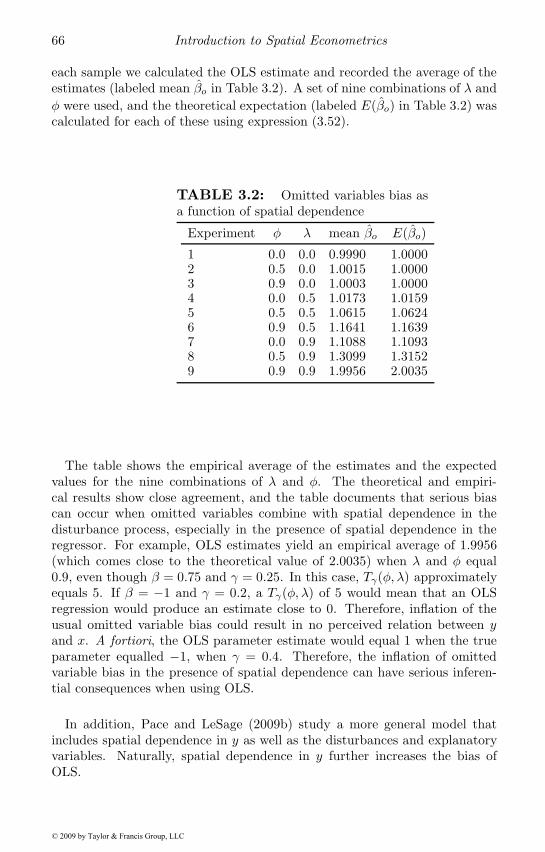
66 Introduction to Spatial Econometrics
each sample we calculated the OLS estimate and recorded the average of theestimates (labeled mean βo in Table 3.2). A set of nine combinations of λ andφ were used, and the theoretical expectation (labeled E(βo) in Table 3.2) wascalculated for each of these using expression (3.52).
TABLE 3.2: Omitted variables bias asa function of spatial dependence
Experiment φ λ mean βo E(βo)
1 0.0 0.0 0.9990 1.00002 0.5 0.0 1.0015 1.00003 0.9 0.0 1.0003 1.00004 0.0 0.5 1.0173 1.01595 0.5 0.5 1.0615 1.06246 0.9 0.5 1.1641 1.16397 0.0 0.9 1.1088 1.10938 0.5 0.9 1.3099 1.31529 0.9 0.9 1.9956 2.0035
The table shows the empirical average of the estimates and the expectedvalues for the nine combinations of λ and φ. The theoretical and empiri-cal results show close agreement, and the table documents that serious biascan occur when omitted variables combine with spatial dependence in thedisturbance process, especially in the presence of spatial dependence in theregressor. For example, OLS estimates yield an empirical average of 1.9956(which comes close to the theoretical value of 2.0035) when λ and φ equal0.9, even though β = 0.75 and γ = 0.25. In this case, Tγ(φ, λ) approximatelyequals 5. If β = −1 and γ = 0.2, a Tγ(φ, λ) of 5 would mean that an OLSregression would produce an estimate close to 0. Therefore, inflation of theusual omitted variable bias could result in no perceived relation between yand x. A fortiori, the OLS parameter estimate would equal 1 when the trueparameter equalled −1, when γ = 0.4. Therefore, the inflation of omittedvariable bias in the presence of spatial dependence can have serious inferen-tial consequences when using OLS.
In addition, Pace and LeSage (2009b) study a more general model thatincludes spatial dependence in y as well as the disturbances and explanatoryvariables. Naturally, spatial dependence in y further increases the bias ofOLS.
© 2009 by Taylor & Francis Group, LLC
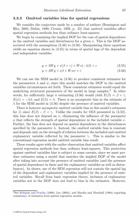
Maximum Likelihood Estimation 67
3.3.3 Omitted variables bias for spatial regressions
We consider the conjecture made by a number of authors (Brasington andHite, 2005; Dubin, 1988; Cressie, 1993, p. 25) that omitted variables affectspatial regression methods less than ordinary least-squares.
We begin by examining the implied DGP for the case of spatial dependencein the omitted variables and disturbances for a given x. This is the DGP as-sociated with the assumptions (3.48) to (3.50). Manipulating these equationsyields an equation shown in (3.55) in terms of spatial lags of the dependentand independent variables.
y = λWy + x(β + γ) +Wx(−λβ) + ε (3.55)y = λWy + xβ +Wxψ + ε (3.56)
We can use the SDM model in (3.56) to produce consistent estimates forthe parameters λ and ψ, since this model matches the DGP in the omittedvariables circumstances set forth. These consistent estimates would equal theunderlying structural parameters of the model in large samples.3 In otherwords, for sufficiently large n estimating (3.56) would yield E(β) = β + γ,E(ψ) = −λβ, and E(λ) = λ. There is no asymptotic bias in the estimate ofλ for the SDM model in (3.56) despite the presence of omitted variables.
There is however asymptotic omitted variable bias in this model’s estimatesfor β, since E(β) − β = γ. Unlike the results for OLS presented in (3.52),this bias does not depend on x, eliminating the influence of the parameterφ that reflects the strength of spatial dependence in the included variable x.Further, the bias does not depend on spatial dependence in the disturbancesspecified by the parameter λ. Instead, the omitted variable bias is constantand depends only on the strength of relation between the included and omittedexplanatory variable reflected by the parameter γ. This is similar to theconventional regression model omitted variable bias result.
These results agree with the earlier observation that omitted variables affectspatial regression methods less than ordinary least-squares. This protectionagainst omitted variables bias is subject to some caveats, since we must pro-duce estimates using a model that matches the implied DGP of the modelafter taking into account the presence of omitted variables (and the presenceof spatial dependence in these and the explanatory variables as well as distur-bances). As shown, use of the SEM regression will not contain the spatial lagof the dependent and explanatory variables implied by the presence of omit-ted variables. Recall from basic regression theory, inclusion of explanatoryvariables not in the DGP does not lead to bias in the estimates. However,
3See Kelejian and Prucha (1998), Lee (2004), and Mardia and Marshall (1984) regardingconsistency of estimates from spatial regression models.
© 2009 by Taylor & Francis Group, LLC
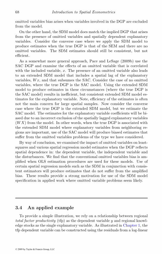
68 Introduction to Spatial Econometrics
omitted variables bias arises when variables involved in the DGP are excludedfrom the model.
On the other hand, the SDM model does match the implied DGP that arisesfrom the presence of omitted variables and spatially dependent explanatoryvariables. Consider the converse case where we apply the SDM model toproduce estimates when the true DGP is that of the SEM and there are noomitted variables. The SDM estimates should still be consistent, but notefficient.
As a somewhat more general approach, Pace and LeSage (2009b) use theSAC DGP and examine the effects of an omitted variable that is correlatedwith the included variable, x. The presence of an omitted variable also leadsto an extended SDM model that includes a spatial lag of the explanatoryvariables, Wx, and that subsumes the SAC. Consider the case of no omittedvariables, where the true DGP is the SAC model. Using the extended SDMmodel to produce estimates in these circumstances (where the true DGP isthe SAC model) results in inefficient, but consistent extended SDM model es-timates for the explanatory variable. Note, efficiency of the estimates is oftennot the main concern for large spatial samples. Now consider the conversecase where the true DGP is the extended SDM model, but we estimate theSAC model. The estimates for the explanatory variable coefficients will be bi-ased due to an incorrect exclusion of the spatially lagged explanatory variables(WX) from the model. In other words, when the true DGP is associated withthe extended SDM model where explanatory variables from neighboring re-gions are important, use of the SAC model will produce biased estimates thatsuffer from the omitted variables problems of the type we have considered.
By way of conclusion, we examined the impact of omitted variables on least-squares and various spatial regression model estimates when the DGP reflectsspatial dependence in: the dependent variable, the independent variable andthe disturbances. We find that the conventional omitted variables bias is am-plified when OLS estimation procedures are used for these models. Use ofcertain spatial regression models such as the SDM in conjunction with consis-tent estimators will produce estimates that do not suffer from the amplifiedbias. These results provide a strong motivation for use of the SDM modelspecification in applied work where omitted variable problems seem likely.
3.4 An applied example
To provide a simple illustration, we rely on a relationship between regionaltotal factor productivity (tfp) as the dependent variable y and regional knowl-edge stocks as the single explanatory variable. As illustrated in Chapter 1, thetfp dependent variable can be constructed using the residuals from a log-linear
© 2009 by Taylor & Francis Group, LLC
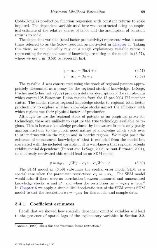
Maximum Likelihood Estimation 69
Cobb-Douglas production function regression with constant returns to scaleimposed. The dependent variable used here was constructed using an empir-ical estimate of the relative shares of labor and the assumption of constantreturns to scale.
The dependent variable (total factor productivity) represents what is some-times referred to as the Solow residual, as motivated in Chapter 1. Takingthis view, we can plausibly rely on a single explanatory variable vector Arepresenting the regional stock of knowledge, resulting in the model in (3.57),where we use a in (3.58) to represent lnA.
y = αιn + βlnA+ ε (3.57)y = αιn + βa+ ε (3.58)
The variable A was constructed using the stock of regional patents appro-priately discounted as a proxy for the regional stock of knowledge. LeSage,Fischer and Scherngell (2007) provide a detailed description of the sample datawhich covers 198 European Union regions from the 15 pre-2004 EU memberstates. The model relates regional knowledge stocks to regional total factorproductivity to explore whether knowledge stocks impact the efficiency withwhich regions use their physical factors of production.
Although we use the regional stock of patents as an empirical proxy fortechnology, these are unlikely to capture the true technology available to re-gions. This is because knowledge produced by innovative firms is only partlyappropriated due to the public good nature of knowledge which spills overto other firms within the region and in nearby regions. We might posit theexistence of unmeasured knowledge a∗ that is excluded from the model butcorrelated with the included variable a. It is well-known that regional patentsexhibit spatial dependence (Parent and LeSage, 2008; Autant-Bernard, 2001),so as already motivated this would lead to an SDM model:
y = α0ιn + ρWy + α1a+ α2Wa+ ε (3.59)
The SDM model in (3.59) subsumes the spatial error model SEM as aspecial case when the parameter restriction: α2 = −ρα1. The SEM modelwould arise if there were no correlation between measured and unmeasuredknowledge stocks, a and a∗, and when the restriction α2 = −ρα1 is true.4
In Chapter 6 we apply a simple likelihood-ratio test of the SEM versus SDMmodel to test the restriction α2 = −ρα1 for this model and sample data.
3.4.1 Coefficient estimates
Recall that we showed how spatially dependent omitted variables will leadto the presence of spatial lags of the explanatory variables in Section 2.2.
4Anselin (1988) labels this the “common factor restriction.”
© 2009 by Taylor & Francis Group, LLC
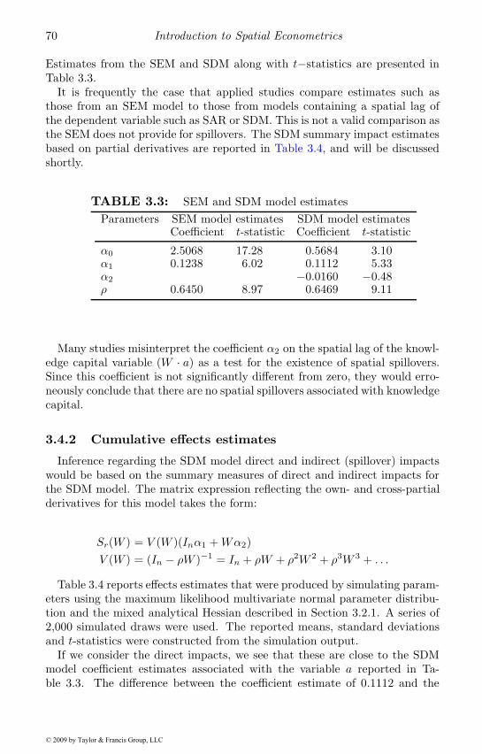
70 Introduction to Spatial Econometrics
Estimates from the SEM and SDM along with t−statistics are presented inTable 3.3.
It is frequently the case that applied studies compare estimates such asthose from an SEM model to those from models containing a spatial lag ofthe dependent variable such as SAR or SDM. This is not a valid comparison asthe SEM does not provide for spillovers. The SDM summary impact estimatesbased on partial derivatives are reported in Table 3.4, and will be discussedshortly.
TABLE 3.3: SEM and SDM model estimatesParameters SEM model estimates SDM model estimates
Coefficient t-statistic Coefficient t-statistic
α0 2.5068 17.28 0.5684 3.10α1 0.1238 6.02 0.1112 5.33α2 −0.0160 −0.48ρ 0.6450 8.97 0.6469 9.11
Many studies misinterpret the coefficient α2 on the spatial lag of the knowl-edge capital variable (W · a) as a test for the existence of spatial spillovers.Since this coefficient is not significantly different from zero, they would erro-neously conclude that there are no spatial spillovers associated with knowledgecapital.
3.4.2 Cumulative effects estimates
Inference regarding the SDM model direct and indirect (spillover) impactswould be based on the summary measures of direct and indirect impacts forthe SDM model. The matrix expression reflecting the own- and cross-partialderivatives for this model takes the form:
Sr(W ) = V (W )(Inα1 +Wα2)V (W ) = (In − ρW )−1 = In + ρW + ρ2W 2 + ρ3W 3 + . . .
Table 3.4 reports effects estimates that were produced by simulating param-eters using the maximum likelihood multivariate normal parameter distribu-tion and the mixed analytical Hessian described in Section 3.2.1. A series of2,000 simulated draws were used. The reported means, standard deviationsand t-statistics were constructed from the simulation output.
If we consider the direct impacts, we see that these are close to the SDMmodel coefficient estimates associated with the variable a reported in Ta-ble 3.3. The difference between the coefficient estimate of 0.1112 and the
© 2009 by Taylor & Francis Group, LLC
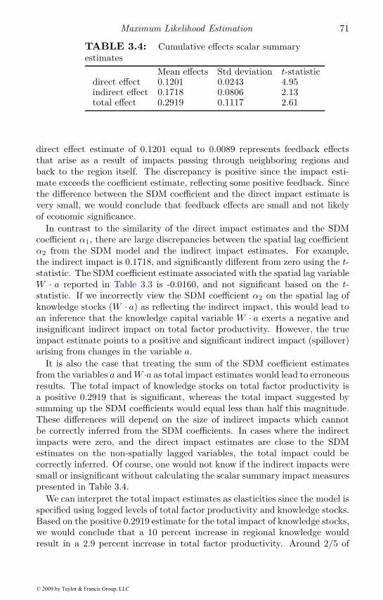
Maximum Likelihood Estimation 71
TABLE 3.4: Cumulative effects scalar summaryestimates
Mean effects Std deviation t-statisticdirect effect 0.1201 0.0243 4.95indirect effect 0.1718 0.0806 2.13total effect 0.2919 0.1117 2.61
direct effect estimate of 0.1201 equal to 0.0089 represents feedback effectsthat arise as a result of impacts passing through neighboring regions andback to the region itself. The discrepancy is positive since the impact esti-mate exceeds the coefficient estimate, reflecting some positive feedback. Sincethe difference between the SDM coefficient and the direct impact estimate isvery small, we would conclude that feedback effects are small and not likelyof economic significance.
In contrast to the similarity of the direct impact estimates and the SDMcoefficient α1, there are large discrepancies between the spatial lag coefficientα2 from the SDM model and the indirect impact estimates. For example,the indirect impact is 0.1718, and significantly different from zero using the t-statistic. The SDM coefficient estimate associated with the spatial lag variableW · a reported in Table 3.3 is -0.0160, and not significant based on the t-statistic. If we incorrectly view the SDM coefficient α2 on the spatial lag ofknowledge stocks (W · a) as reflecting the indirect impact, this would lead toan inference that the knowledge capital variable W · a exerts a negative andinsignificant indirect impact on total factor productivity. However, the trueimpact estimate points to a positive and significant indirect impact (spillover)arising from changes in the variable a.
It is also the case that treating the sum of the SDM coefficient estimatesfrom the variables a andW ·a as total impact estimates would lead to erroneousresults. The total impact of knowledge stocks on total factor productivity isa positive 0.2919 that is significant, whereas the total impact suggested bysumming up the SDM coefficients would equal less than half this magnitude.These differences will depend on the size of indirect impacts which cannotbe correctly inferred from the SDM coefficients. In cases where the indirectimpacts were zero, and the direct impact estimates are close to the SDMestimates on the non-spatially lagged variables, the total impact could becorrectly inferred. Of course, one would not know if the indirect impacts weresmall or insignificant without calculating the scalar summary impact measurespresented in Table 3.4.
We can interpret the total impact estimates as elasticities since the model isspecified using logged levels of total factor productivity and knowledge stocks.Based on the positive 0.2919 estimate for the total impact of knowledge stocks,we would conclude that a 10 percent increase in regional knowledge wouldresult in a 2.9 percent increase in total factor productivity. Around 2/5 of
© 2009 by Taylor & Francis Group, LLC
72 Introduction to Spatial Econometrics
this impact comes from the direct effect magnitude of 0.1201, and 3/5 fromthe indirect or spatial spillover impact based on its scalar impact estimate of0.1718.
3.4.3 Spatial partitioning of the impact estimates
We can spatially partition these impacts to illustrate the nature of theirinfluence as we move from immediate to higher-order neighbors. This mightbe of interest in applications where the spatial extent of the spillovers is anobject of inference.
These are presented for the SDM model in Table 3.5, which shows themean, standard deviation and a t-statistic for the marginal effects associatedwith matrices W of orders 0 to 9. Direct effects for W 1 will equal zero andthe indirect effects for W 0 equal zero as discussed in Chapter 2. Of course,if we cumulated the marginal effects in the table over all orders of W untilempirical convergence of the infinite series, these would equal the cumulativeeffects reported in Table 3.4.
TABLE 3.5: Marginal spatial partitioning ofimpacts
Direct effects Standard deviation t-statisticW 0 0.1113 0.0205 5.4191W 1 0.0000 0.0000 —W 2 0.0046 0.0013 3.5185W 3 0.0016 0.0007 2.3739W 4 0.0010 0.0005 2.0147W 5 0.0006 0.0003 1.6643W 6 0.0004 0.0002 1.4208W 7 0.0002 0.0002 1.2285W 8 0.0001 0.0001 1.0761W 9 0.0001 0.0001 0.9516
Indirect effects Standard deviation t-statisticW 0 0.0000 0.0000 —W 1 0.0622 0.0188 3.3085W 2 0.0353 0.0131 2.6985W 3 0.0243 0.0105 2.3098W 4 0.0160 0.0083 1.9220W 5 0.0107 0.0066 1.6283W 6 0.0072 0.0052 1.3978W 7 0.0049 0.0040 1.2151W 8 0.0033 0.0031 1.0672W 9 0.0023 0.0024 0.9455
© 2009 by Taylor & Francis Group, LLC
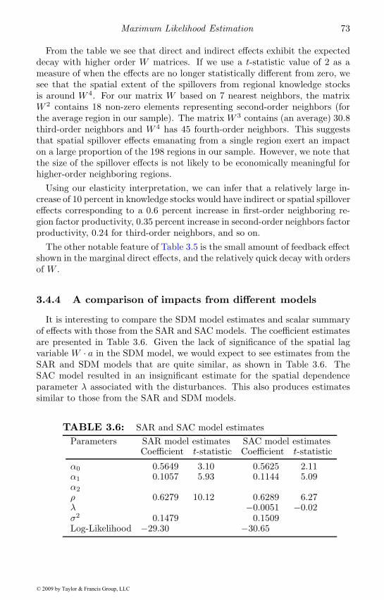
Maximum Likelihood Estimation 73
From the table we see that direct and indirect effects exhibit the expecteddecay with higher order W matrices. If we use a t-statistic value of 2 as ameasure of when the effects are no longer statistically different from zero, wesee that the spatial extent of the spillovers from regional knowledge stocksis around W 4. For our matrix W based on 7 nearest neighbors, the matrixW 2 contains 18 non-zero elements representing second-order neighbors (forthe average region in our sample). The matrix W 3 contains (an average) 30.8third-order neighbors and W 4 has 45 fourth-order neighbors. This suggeststhat spatial spillover effects emanating from a single region exert an impacton a large proportion of the 198 regions in our sample. However, we note thatthe size of the spillover effects is not likely to be economically meaningful forhigher-order neighboring regions.
Using our elasticity interpretation, we can infer that a relatively large in-crease of 10 percent in knowledge stocks would have indirect or spatial spillovereffects corresponding to a 0.6 percent increase in first-order neighboring re-gion factor productivity, 0.35 percent increase in second-order neighbors factorproductivity, 0.24 for third-order neighbors, and so on.
The other notable feature of Table 3.5 is the small amount of feedback effectshown in the marginal direct effects, and the relatively quick decay with ordersof W .
3.4.4 A comparison of impacts from different models
It is interesting to compare the SDM model estimates and scalar summaryof effects with those from the SAR and SAC models. The coefficient estimatesare presented in Table 3.6. Given the lack of significance of the spatial lagvariable W · a in the SDM model, we would expect to see estimates from theSAR and SDM models that are quite similar, as shown in Table 3.6. TheSAC model resulted in an insignificant estimate for the spatial dependenceparameter λ associated with the disturbances. This also produces estimatessimilar to those from the SAR and SDM models.
TABLE 3.6: SAR and SAC model estimatesParameters SAR model estimates SAC model estimates
Coefficient t-statistic Coefficient t-statistic
α0 0.5649 3.10 0.5625 2.11α1 0.1057 5.93 0.1144 5.09α2
ρ 0.6279 10.12 0.6289 6.27λ −0.0051 −0.02σ2 0.1479 0.1509Log-Likelihood −29.30 −30.65
© 2009 by Taylor & Francis Group, LLC
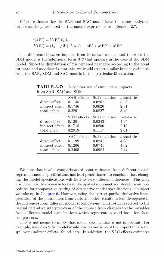
74 Introduction to Spatial Econometrics
Effects estimates for the SAR and SAC model have the same analyticalform since they are based on the matrix expressions from Section 2.7.
Sr(W ) = V (W )InβrV (W ) = (In − ρW )−1 = In + ρW + ρ2W 2 + ρ3W 3 + . . .
The difference between impacts from these two models and those for theSDM model is the additional term Wθ that appears in the case of the SDMmodel. Since the distribution of θ is centered near zero according to the pointestimate and associated t-statistic, we would expect similar impact estimatesfrom the SAR, SDM and SAC models in this particular illustration.
TABLE 3.7: A comparison of cumulative impactsfrom SAR, SAC and SDM
SAR effects Std deviation t-statisticdirect effect 0.1145 0.0207 5.53indirect effect 0.1746 0.0620 2.81total effect 0.2891 0.0827 3.49
SDM effects Std deviation t-statisticdirect effect 0.1201 0.0243 4.95indirect effect 0.1718 0.0806 2.13total effect 0.2919 0.1117 2.61
SAC effects Std deviation t-statisticdirect effect 0.1199 0.0241 4.98indirect effect 0.1206 0.0741 1.62total effect 0.2405 0.0982 2.44
We note that invalid comparisons of point estimates from different spatialregression model specifications has lead practitioners to conclude that chang-ing the model specifications will lead to very different inferences. This mayalso have lead to excessive focus in the spatial econometrics literature on pro-cedures for comparative testing of alternative model specifications, a subjectwe take up in Chapter 6. However, using the correct partial derivative inter-pretation of the parameters from various models results in less divergence inthe inferences from different model specifications. This result is related to thepartial derivative interpretation of the impact from changes to the variablesfrom different model specifications which represents a valid basis for thesecomparisons.
This is not meant to imply that model specification is not important. Forexample, use of an SEM model would lead to omission of the important spatialspillover (indirect effects) found here. In addition, the SAC effects estimates
© 2009 by Taylor & Francis Group, LLC
Maximum Likelihood Estimation 75
lead to an inference that the indirect spillover impacts are not significantlydifferent from zero based on the t-statistic reported in Table 3.7.
3.5 Chapter summary
In Section 3.1 we set forth computationally efficient approaches to maxi-mum likelihood estimation of the basic family of spatial regression models.The most challenging part of maximum likelihood estimation is computingthe log determinant term that appears in the log-likelihood function, andChapter 4 will provide details regarding this. In addition to point estimatesthere is also a need to provide a variance-covariance matrix estimate thatcan be used for inference. Section 3.2 discussed various strategies and setforth a mixed approach that uses numerical Hessian results to modify a singlecomputationally challenging term from the analytical Hessian.
The public domain Spatial Econometrics Toolbox (LeSage, 2007) and SpatialStatistics Toolbox (Pace, 2007) provide code examples written in the MAT-LAB language that implement most of the methods discussed in this text.This should allow the interested reader to examine detailed examples thatimplement the ideas presented here.
Modeling spatial relationships often results in omitted latent influences thatare spatial in nature. For example, hedonic home price regressions usuallyrely on individual house characteristics that may exclude important neigh-borhood variables that reflect accessibility, school quality, amenities, etc. InSection 3.3, we examined the nature of bias that will arise from omitted vari-ables in both least-squares and spatial regression estimates. An interestingfeature of omitted variables in spatial regression models is that they will leadto data generating processes that include spatial lags of the explanatory vari-ables, providing a powerful motivation for use of the spatial Durbin model.
An applied illustration was provided in Section 3.4 to reinforce the ideasset forth in this chapter. A comparison of maximum likelihood estimatesfrom a family of spatial regression models along with an interpretation ofthe parameters was provided. The simple one-variable model was based onregional variation in factor productivity for a sample of 198 European Unionregions. The focus of this applied illustration was on the role of regionalknowledge stocks in explaining variation in regional total factor productivity.
© 2009 by Taylor & Francis Group, LLC
Chapter 4
Log-determinants and SpatialWeights
Many spatial applications involve large data sets. For example, the US Censusprovides data on blocks (n = 8, 205, 582), block groups (n = 208, 790), censustracts (n = 65, 443), and other geographies. In the case of the Census data,each of these observations represents a region. If spatial dependence is mate-rial and each region affects every other region, this leads to n×n dependencerelations. Since some applications involve elaborate models, computationalaspects of spatial econometrics have been an active area of research for sometime (Ord, 1975; Martin, 1993; Pace and Barry, 1997; Griffith, 2000; Smirnovand Anselin, 2001; LeSage and Pace, 2007).
This chapter addresses theoretical and numerical issues that arise whenfitting models to spatial data using likelihood-based techniques. Likelihood-based techniques involve the determinant of the variance-covariance matrixwhich measures the degree of dependence among observations. This chapteraddresses both exact and approximate calculation of the log-determinant andbounds for the dependence parameter.
In addition, the chapter deals with calculation of other quantities usedin spatial estimation and inference such as the diagonal of the variance-covariance matrix and the derivative of the log-determinant.
The chapter addresses efficient computation of the estimated spatial effectsand shows a general approach to obtaining closed-form solutions to manysingle parameter spatial models. Finally, the chapter discusses aspects ofquickly constructing spatial weight matrices.
4.1 Determinants and transformations
Statistical applications often involve transformations of the dependent vari-able. Unless these transformations are handled properly, statistical procedureshave the potential to produce pathological behavior. We use a simple exampleto illustrate the type of problem that can arise. Suppose the interest is in aleast-squares fit of the relationship in (4.1) involving transformation of thedependent variable by the scalar T .
77© 2009 by Taylor & Francis Group, LLC
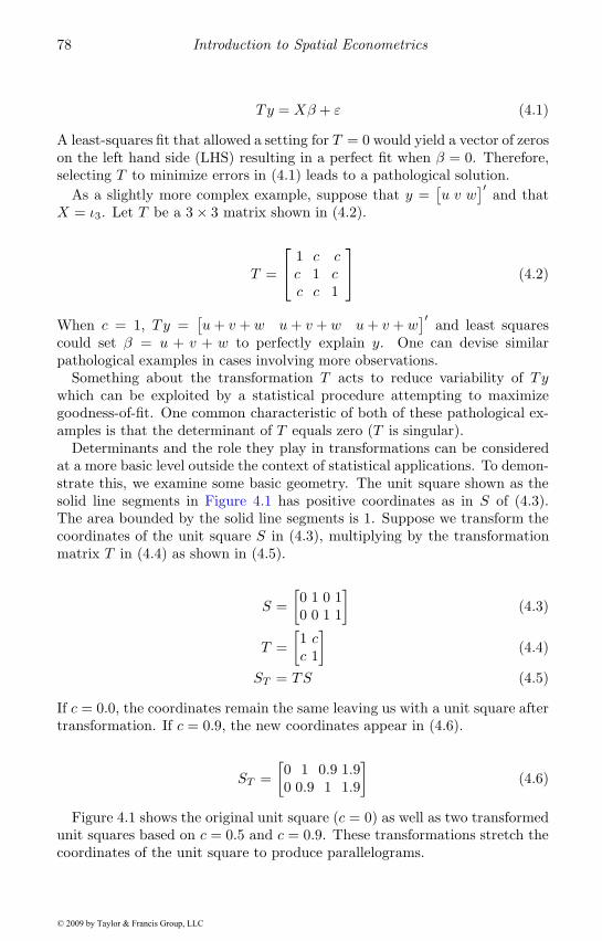
78 Introduction to Spatial Econometrics
Ty = Xβ + ε (4.1)
A least-squares fit that allowed a setting for T = 0 would yield a vector of zeroson the left hand side (LHS) resulting in a perfect fit when β = 0. Therefore,selecting T to minimize errors in (4.1) leads to a pathological solution.
As a slightly more complex example, suppose that y =[u v w
]′ and thatX = ι3. Let T be a 3 × 3 matrix shown in (4.2).
T =
⎡⎣ 1 c cc 1 cc c 1
⎤⎦ (4.2)
When c = 1, Ty =[u+ v + w u+ v + w u+ v + w
]′ and least squarescould set β = u + v + w to perfectly explain y. One can devise similarpathological examples in cases involving more observations.
Something about the transformation T acts to reduce variability of Tywhich can be exploited by a statistical procedure attempting to maximizegoodness-of-fit. One common characteristic of both of these pathological ex-amples is that the determinant of T equals zero (T is singular).
Determinants and the role they play in transformations can be consideredat a more basic level outside the context of statistical applications. To demon-strate this, we examine some basic geometry. The unit square shown as thesolid line segments in Figure 4.1 has positive coordinates as in S of (4.3).The area bounded by the solid line segments is 1. Suppose we transform thecoordinates of the unit square S in (4.3), multiplying by the transformationmatrix T in (4.4) as shown in (4.5).
S =[0 1 0 10 0 1 1
](4.3)
T =[1 cc 1
](4.4)
ST = TS (4.5)
If c = 0.0, the coordinates remain the same leaving us with a unit square aftertransformation. If c = 0.9, the new coordinates appear in (4.6).
ST =[0 1 0.9 1.90 0.9 1 1.9
](4.6)
Figure 4.1 shows the original unit square (c = 0) as well as two transformedunit squares based on c = 0.5 and c = 0.9. These transformations stretch thecoordinates of the unit square to produce parallelograms.
© 2009 by Taylor & Francis Group, LLC
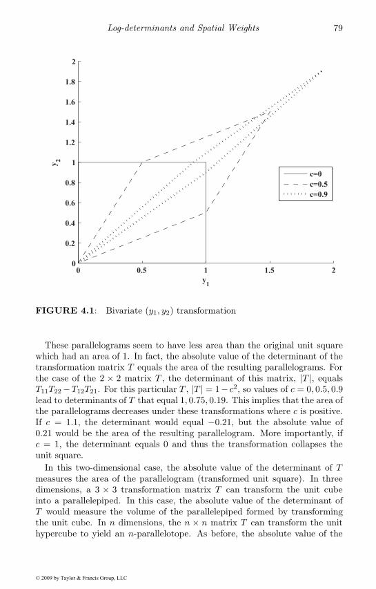
Log-determinants and Spatial Weights 79
0 0.5 1 1.5 20
0.2
0.4
0.6
0.8
1
1.2
1.4
1.6
1.8
2
y1
y2
c=0
c=0.5
c=0.9
FIGURE 4.1: Bivariate (y1, y2) transformation
These parallelograms seem to have less area than the original unit squarewhich had an area of 1. In fact, the absolute value of the determinant of thetransformation matrix T equals the area of the resulting parallelograms. Forthe case of the 2 × 2 matrix T , the determinant of this matrix, |T |, equalsT11T22 −T12T21. For this particular T , |T | = 1− c2, so values of c = 0, 0.5, 0.9lead to determinants of T that equal 1, 0.75, 0.19. This implies that the area ofthe parallelograms decreases under these transformations where c is positive.If c = 1.1, the determinant would equal −0.21, but the absolute value of0.21 would be the area of the resulting parallelogram. More importantly, ifc = 1, the determinant equals 0 and thus the transformation collapses theunit square.
In this two-dimensional case, the absolute value of the determinant of Tmeasures the area of the parallelogram (transformed unit square). In threedimensions, a 3 × 3 transformation matrix T can transform the unit cubeinto a parallelepiped. In this case, the absolute value of the determinant ofT would measure the volume of the parallelepiped formed by transformingthe unit cube. In n dimensions, the n × n matrix T can transform the unithypercube to yield an n-parallelotope. As before, the absolute value of the
© 2009 by Taylor & Francis Group, LLC
80 Introduction to Spatial Econometrics
determinant of T would measure the n-dimensional volume.
Returning to statistical issues, examine the point clouds in Figure 4.2 froma transformed normal bivariate distribution based on varying the level ofcorrelation between y1 and y2, which we denote ρ = 0, 0.33, 0.66, 0.99. Thebivariate distribution before the transformation was proper (the volume underthe bivariate density equals 1). These point clouds show a pattern similar tothat of the parallelograms with higher correlations corresponding to moresevere transformations.
5 0 54
2
0
2
4
ρ=0
y1
y2
4 2 0 2 4 4
2
0
2
4
ρ=0.33
y1
y2
4 2 0 2 4 4
2
0
2
4
ρ=0.66
y1
y2
5 0 5 6
4
2
0
2
4
ρ=0.99
y1
y2
FIGURE 4.2: Bivariate (y1, y2) normal point clouds by correlation (ρ)
It is visually evident that the point clouds associated with the transforma-tions exhibit shrinkage relative to the original point cloud. To counteract theshrinkage aspect of transformations, distributions must include an adjustmentto preserve the volume of unity under the joint probability density. As a re-sult, continuous multivariate densities such as the multivariate normal in (4.7)include the determinant of the variance-covariance matrix as the adjustment.
© 2009 by Taylor & Francis Group, LLC
Log-determinants and Spatial Weights 81
N(u) = (2π)−n/2|Ω|−1/2 exp(
12(u− μ)′Ω−1(u− μ)
)(4.7)
The multivariate t distribution (shown below), Wishart, and other distri-butions also contain a determinant term.
t(u) = Γ(n+ p
2
)Γ(n
2
)−1
(nπ)−p2 |Ω|− 1
2
(1 +
(u− μ)′Ω−1(u− μ)n
)−n+p2
4.2 Basic determinant computation
The product of the diagonal elements of a triangular or a diagonal ma-trix yields the determinant. Most algorithms for calculating the determinantexploit this by reducing the matrix under consideration to a diagonal or atriangular matrix. There are various approaches that can be used to create di-agonal or triangular matrices. For example, one can compute the determinantof a matrix using eigenvalues which reduce the matrix under consideration toa diagonal matrix. Alternatively, various forms of Gaussian elimination suchas the LU or Cholesky decompositions reduce the matrix under considerationto a triangular matrix. These matrix decomposition techniques also use themultiplicative property of determinants, |CD| = |C||D| to reduce the generalproblem to a product involving simpler problems.
The matrix decomposition approach to calculating determinants can beillustrated with simple examples. We begin with the Gaussian eliminationapproach which relies on elementary operations such as adding a multiple ofone row to another to achieve a triangular form. These row operations donot change the determinant, and therefore the final triangular matrix has thesame determinant as the initial matrix of interest. We begin with A in (4.8)and add the first row of A times a to the second row of A, which zeros outthe element below the diagonal yielding A1 in (4.9). The diagonal elementsof the resulting triangular matrix A1 are known as pivots, and the product ofthe pivots equals the determinant as shown in (4.10) (Strang, 1976).
A =[
1 −a−a 1
](4.8)
A1 =[1 −a0 1 − a2
](4.9)
|A| = |A1| = 1 − a2 (4.10)
© 2009 by Taylor & Francis Group, LLC
82 Introduction to Spatial Econometrics
A zero pivot would yield a zero determinant and a singular matrix. Therefore,non-singular matrices yield non-zero pivots and positive definite matrices yieldstrictly positive pivots. Obviously, A is non-singular when abs(a) �= 1 and Ais positive definite when abs(a) < 1.
Note, the determinant of the first sub-matrix of A or A11 equals 1. Notcoincidentally, this is the first pivot of A1. In fact, the pivots from the trian-gular matrix produced by row operations yield the sequence of determinantsfor sub-matrices of increasing size. This is a valuable feature that is usefulin examining spatial systems composed of subsets of the observations such asused in local spatial autoregressions (Pace and LeSage, 2003a).
Most computer routines actually yield a unit lower triangular matrix L con-taining ones on the diagonal, an upper triangular matrix U and a permutationmatrix P so that PA = LU . The result of PA is to reorder the rows of A.This can be used to produce |A| = |L||U |/|P |, which represents an LU de-composition with permutations or reordering of rows for numerical accuracy.Fortunately, when A = In−ρW where W is row-stochastic and abs(ρ) < 1, Ais strictly diagonally dominant. This means that the diagonal element (whichequals 1) strictly exceeds the sum of the other elements in the row (whichequals ρ since W is row-stochastic). Strictly diagonally dominant matricesare invertible (non-singular). Moreover, strictly diagonally dominant matri-ces do not require reordering rows of A, allowing us to set P = In (Golub andVan Loan, 1996, Theorem 3.4.3). For the case where P = In, L is unit lowertriangular having a determinant of 1, so |A| = |U | (Strang, 1976, p. 21).
For symmetric positive definite matrices, an algorithmic variant yields theCholesky decomposition so that A = R′R where R is triangular. Therefore|A| = |R||R′| = |R|2, since the determinant of a matrix and its transposeare identical. The Cholesky decomposition is almost twice as fast as the LUdecomposition since it takes account of symmetry. In addition, symmetricpositive definite matrices do not require reordering or permutations for nu-merical accuracy which reduces the computational cost.
For non-symmetric A interest often lies in B = A′A. In this case, a non-singular A implies a symmetric positive definite B. Therefore, it sometimespays to find the determinant of the symmetric B rather than work directlywith A. In this case, non-singular A can have negative (but not zero) ele-ments on the diagonal of U . The determinant of A equals the product ofthe pivots (some of which may be positive and others negative) and thus canbe positive or negative. This creates a problem when calculating the log ofthe determinant for B. However, this problem can be resolved by taking theabsolute value of the determinant which implies finding the absolute value ofthe pivots before using logs as shown in (4.11) to (4.13).
© 2009 by Taylor & Francis Group, LLC
Log-determinants and Spatial Weights 83
|B| = |A′||A| = abs(|A|)2 (4.11)
abs(|A|) =n∏i=1
abs(Uii) (4.12)
ln |B| = 2 ln abs(|A|) = 2n∑i=1
ln(abs(Uii)) (4.13)
For symmetric real matrices (or those that can be transformed to exhibitsymmetry), one can obtain the spectral decomposition B = V ΛBV ′. Thisdecomposition was applied to our 2× 2 example to produce the results shownin (4.17) and (4.18). The diagonal matrix ΛB contains the n real eigenvalues,and V in (4.17) is a matrix comprised of n orthogonal eigenvectors (eachwith n elements). By construction, V V ′ = In and this sets up (4.19). Since|V | = |V ′|, it follows that |V | = |V ′| = 1 and this allows us to find thedeterminant using the product of the diagonal elements of I2 − aΛB as shownin (4.21). This is equal to the usual 2 × 2 determinant expression which canbe seen from (4.22).
A = I2 − aB (4.14)
B =[0 11 0
](4.15)
B = V ΛBV ′ (4.16)
V =[−0.7071 −0.7071−0.7071 0.7071
](4.17)
ΛB =[−1 0
0 1
](4.18)
A = V (I2 − aΛB)V ′ (4.19)|A| = |V ||I2 − aΛB||V ′| (4.20)|A| = (1 − aΛ11)(1 − aΛ22) (4.21)|A| = (1 + a)(1 − a) = 1 − a2 (4.22)
An advantage of the eigenvalue approach is that the eigenvalues of B onlyneed to be computed once. Subsequent updating of the determinant of A fordiffering values of a requires very little additional computation. However, theeigenvalue approach does not scale well to larger problems.
In terms of computation, all of these techniques require order of n cubed(O(n3)) calculations for general matrices. However, the Cholesky requiresn3/3, the LU requires 2n3/3. There are many methods for calculating eigen-values which require a multiple of the LU and Cholesky counts since themethods have some iterative component.
© 2009 by Taylor & Francis Group, LLC
84 Introduction to Spatial Econometrics
In practice, it becomes numerically challenging to compute the actual de-terminant using the product of all pivots, since small pivots can lead to a verysmall numerically inaccurate determinant. Instead of calculating the deter-minant per se, we can find the log-determinant using the sum of the loggedpivots which will produce a more accurate numerical solution. This naturallyrequires positive pivots such as those from a positive definite matrix.
Some rules pertaining to determinants and related quantities of interest inspatial econometrics are enumerated below. We will discuss their applicationin circumstances specific to various spatial econometric modeling situationsin Section 4.3.
|CD| = |C||D| (4.23)|C′| = |C| (4.24)
|G| =n∏i=1
Gii diagonal or triangular G (4.25)
ln |In − ρW | = −∞∑i=1
ρi tr(W i)i
(4.26)
|eC | = etr(C) (4.27)|Ca| = |C|a (4.28)
|C ⊗D| = |C|dim(D)|D|dim(C) (4.29)tr(C ⊗D) = tr(C) tr(D) (4.30)(C ⊗D)m = Cm ⊗Dm (4.31)
(A⊗B)(C ⊗D) = (AC ⊗BD) (4.32)
tr(Aj) =n∑i=1
λji (4.33)
diag(AB) = (A�B′)ιn (4.34)tr(AB) = ι′n(A�B′)ιn = ι′n(A
′ �B)ιn (4.35)
In the above rules ⊗ represents the Kronecker product and � represents ele-mentwise or Hadamard multiplication.
4.3 Determinants of spatial systems
Spatial models using weight matrices have additional structure and featureswhich greatly aid computation of determinants, equation solutions, and otherquantities of interest for spatial modeling.
© 2009 by Taylor & Francis Group, LLC
Log-determinants and Spatial Weights 85
If each observation depends on some, but not all other n− 1 observations,the weight matrix will have a number of zeros and is therefore a sparse matrix.In particular, the common contiguity weight matrix will have an average ofapproximately six neighbors for each observation for spatially random dataon a plane. An implication is that a contiguity-based weight matrix will haveapproximately 6n non-zeros and n2 − 6n zeros. In terms of the proportionof non-zero elements this equals 6/n, so this matrix becomes increasinglysparse with increasing n. One can generalize this to the m nearest neighborproblem which would have a proportion of non-zeros equal to m/n. Sparsityalso extends to other dependence structures such as those used in geostatistics(Barry and Pace, 1997).
Sparsity provides tremendous storage and computational advantages. Inthe 2000 US Census there were 65, 443 tracts, 208, 790 block groups, and8, 205, 582 blocks. A dense weight matrix would require 31.90, 324.80, and501, 659.33 gigabytes of storage respectively for these sample sizes. In con-trast, a sparse contiguity matrix would require less than 0.01, 0.03, and 1.10gigabytes of storage for these data samples. In terms of computation, somesparse matrix techniques require only linear in n calculations, whereas densematrix techniques often require calculations that are cubic in n.
In addition, weight matrices have known properties, which can often beused to simplify required calculations (Bavaud, 1998; Martellosio, 2006). Oneexample of this is the row-stochastic matrix W , which results in ρ ∈ [0, 1) asa sufficient condition for non-singular Z = In− ρW . An example where zeroson the main diagonal ofW were used can be found in LeSage and Pace (2007).They show that zeros on the diagonal of W lead to a zero log-determinant forthe matrix exponential spatial specification which we discuss in Chapter 9.This arises since ln |eαW | = 0, where eαW plays the role of the transformationmatrix T in (4.1) in the case of the matrix exponential spatial specification.
To illustrate how known properties of spatial systems can be exploited tocomputational advantage, we use a sample of 3, 107 counties in the continen-tal United States. For our illustrations we use a matrix W based on 6 nearestneighbors constructed using Euclidean distance between points of the pro-jected coordinates.1 Figure 4.3 shows the graph (as in graph theory) whereedges (line segments) between nodes (points) indicate nodes that are neigh-bors. If only one edge is needed, the nodes are first-order neighbors. If t edgesare needed to transverse between nodes, the nodes are t-order neighbors.
Orderings of rows and columns greatly affect decomposition times for sparsespatial weight matrices. Ordering rows and columns corresponds to the op-eration WP = PWP ′ where P is an n × n permutation matrix. Permuta-
1The earth is a three dimensional sphere, but maps are two dimensional. Accordingly, mapscan only approximate the surface of a sphere with error. Map projections attempt to makeuseful two dimensional approximations of the sphere (Snyder and Voxland, 1989). We useda transverse Mercator projection of the latitude and longitude coordinates to arrive at newlocational coordinates such as shown in Figure 4.3.
© 2009 by Taylor & Francis Group, LLC
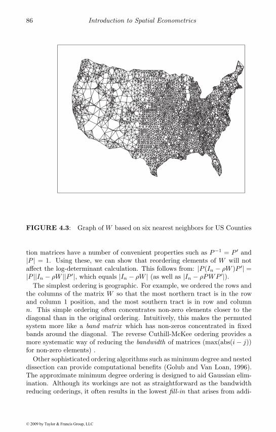
86 Introduction to Spatial Econometrics
FIGURE 4.3: Graph of W based on six nearest neighbors for US Counties
tion matrices have a number of convenient properties such as P−1 = P ′ and|P | = 1. Using these, we can show that reordering elements of W will notaffect the log-determinant calculation. This follows from: |P (In − ρW )P ′| =|P ||In − ρW ||P ′|, which equals |In − ρW | (as well as |In − ρPWP ′|).
The simplest ordering is geographic. For example, we ordered the rows andthe columns of the matrix W so that the most northern tract is in the rowand column 1 position, and the most southern tract is in row and columnn. This simple ordering often concentrates non-zero elements closer to thediagonal than in the original ordering. Intuitively, this makes the permutedsystem more like a band matrix which has non-zeros concentrated in fixedbands around the diagonal. The reverse Cuthill-McKee ordering provides amore systematic way of reducing the bandwidth of matrices (max(abs(i− j))for non-zero elements) .
Other sophisticated ordering algorithms such as minimum degree and nesteddissection can provide computational benefits (Golub and Van Loan, 1996).The approximate minimum degree ordering is designed to aid Gaussian elim-ination. Although its workings are not as straightforward as the bandwidthreducing orderings, it often results in the lowest fill-in that arises from addi-
© 2009 by Taylor & Francis Group, LLC
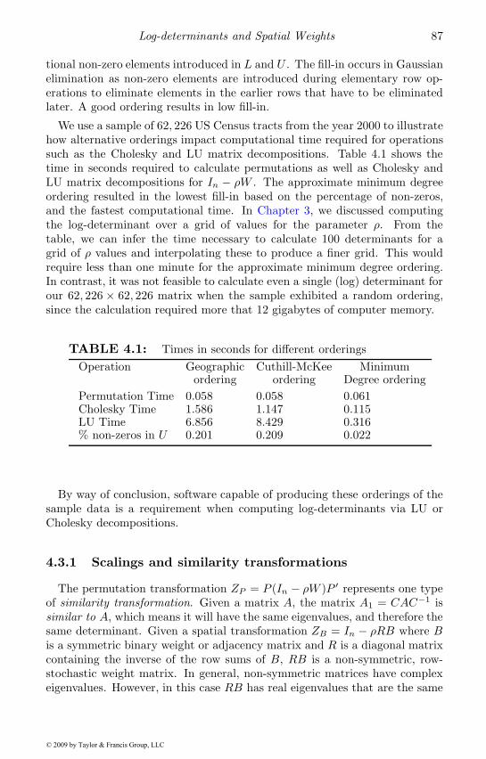
Log-determinants and Spatial Weights 87
tional non-zero elements introduced in L and U . The fill-in occurs in Gaussianelimination as non-zero elements are introduced during elementary row op-erations to eliminate elements in the earlier rows that have to be eliminatedlater. A good ordering results in low fill-in.
We use a sample of 62, 226 US Census tracts from the year 2000 to illustratehow alternative orderings impact computational time required for operationssuch as the Cholesky and LU matrix decompositions. Table 4.1 shows thetime in seconds required to calculate permutations as well as Cholesky andLU matrix decompositions for In − ρW . The approximate minimum degreeordering resulted in the lowest fill-in based on the percentage of non-zeros,and the fastest computational time. In Chapter 3, we discussed computingthe log-determinant over a grid of values for the parameter ρ. From thetable, we can infer the time necessary to calculate 100 determinants for agrid of ρ values and interpolating these to produce a finer grid. This wouldrequire less than one minute for the approximate minimum degree ordering.In contrast, it was not feasible to calculate even a single (log) determinant forour 62, 226 × 62, 226 matrix when the sample exhibited a random ordering,since the calculation required more that 12 gigabytes of computer memory.
TABLE 4.1: Times in seconds for different orderingsOperation Geographic Cuthill-McKee Minimum
ordering ordering Degree orderingPermutation Time 0.058 0.058 0.061Cholesky Time 1.586 1.147 0.115LU Time 6.856 8.429 0.316% non-zeros in U 0.201 0.209 0.022
By way of conclusion, software capable of producing these orderings of thesample data is a requirement when computing log-determinants via LU orCholesky decompositions.
4.3.1 Scalings and similarity transformations
The permutation transformation ZP = P (In − ρW )P ′ represents one typeof similarity transformation. Given a matrix A, the matrix A1 = CAC−1 issimilar to A, which means it will have the same eigenvalues, and therefore thesame determinant. Given a spatial transformation ZB = In − ρRB where Bis a symmetric binary weight or adjacency matrix and R is a diagonal matrixcontaining the inverse of the row sums of B, RB is a non-symmetric, row-stochastic weight matrix. In general, non-symmetric matrices have complexeigenvalues. However, in this case RB has real eigenvalues that are the same
© 2009 by Taylor & Francis Group, LLC
88 Introduction to Spatial Econometrics
as the symmetric (but not row-stochastic) matrix R12BR
12 . Consider the
similarity transformation R− 12ZBR
12 which produces the symmetric matrix
In − ρR12BR
12 . From a statistical perspective, using the row-stochastic RB
may yield better results. However, from a numerical analysis perspectiveusing the similar, but symmetric matrix R
12BR
12 will usually perform better
(Ord, 1975). Therefore, the best strategy in many cases is to use the row-stochasticW for calculations related to the statistical portion of the estimationproblem, but work with a similar symmetric matrix when calculating the log-determinant. Given a table of determinants or the eigenvalues, similaritytransformations represent low-cost computational operations.
Computation is often simpler when W has a maximum eigenvalue of 1,which is the case for row-stochastic matrices or matrices that are similar torow-stochastic matrices. Consider a candidate weight matrix of interest Wa
that does not have a maximum eigenvalue max(λa) equal to 1. This can betransformed using Wb = Wa max(λa)−1 to have a maximum eigenvalue of 1.An implication is that any weight matrix W can be scaled to have a maximumeigenvalue of 1. We note that this facilitates interpretation of the powers ofW , since these would also have a maximum eigenvalue of 1.
Symmetric doubly stochastic weight matrices are those that have rows andcolumns that sum to 1 and exhibit symmetry. This means the maximumeigenvalue equals 1 and all eigenvalues are real. Transforming a matrix Wt todoubly stochastic form involves an iterative process: 1) calculating the diago-nal matrix of row sums Rt for the symmetric weight matrix Wt, 2) calculatingWt+1 = R
− 12
t WtR− 1
2t , and, 3) repeating steps 1) and 2) until convergence. The
resulting doubly stochastic weight matrix is not similar to the initial weightmatrix Wt.
4.3.2 Determinant domain
Which values of ρ lead to non-singular Z = In−ρW? For symmetric matri-ces, the compact open interval for ρ ∈ (λ−1
min, λ−1max) will lead to a symmetric
positive definite Z. In the case of symmetric matrices similar to row-stochasticmatrices where λmax = 1, the interval for ρ becomes (λ−1
min, 1).The situation becomes more difficult when W has complex eigenvalues.
Assume that W is scaled to be row-stochastic so that Wιn = ιn. If W isnot similar to a symmetric matrix, it may have complex eigenvalues. If areal matrix has complex eigenvalues, these come in complex conjugate pairs(Bernstein, 2005, p. 131). Let λ represent the n by 1 vector of eigenvalues ofW . The determinant of (In − ρW ) equals,
|In − ρW | =n∏i=1
(1 − ρλi) =
[n∏i=3
(1 − ρλi)
](1 − ρλ1)(1 − ρλ2) (4.36)
where, without loss of generality, one of the complex conjugate pairs of eigen-
© 2009 by Taylor & Francis Group, LLC
Log-determinants and Spatial Weights 89
values appears in λ1 and the other in λ2. If the product (1 − ρλ1)(1 − ρλ2)equals 0, this would lead to a zero determinant which would imply singular(In − ρW ) and a singular variance-covariance matrix.
What value of ρ could lead to a singular (In−ρW )? To focus on the complexconjugate nature of λ1 and λ2, we express these as λ1 = r+jc and λ2 = r−jc,where r is the real part of λ1, λ2, jc is the complex part of λ1, λ2, and j isthe square root of −1, so that j2 = −1. We assume c �= 0, since a value of 0would lead to a real number representation. Equations (4.37)–(4.40) form thecomplex quadratic equation given complex conjugate pairs of the eigenvaluesand set the complex quadratic equation to 0 to find values of ρ associatedwith a singularity.
0 = (1 − ρλ1)(1 − ρλ2) (4.37)0 = (1 − ρr − ρjc)(1 − ρr + ρjc) (4.38)0 = 1 − 2ρr + ρ2r2 − j2ρ2c2 (4.39)0 = 1 − 2ρr + ρ2(r2 + c2) (4.40)
Rewriting (4.40) using the discriminant d = b2 − 4ac from the quadraticformula ax2 + bx+ c = 0 we find that d < 0.
d = 4[r2 − r2 − c2
](4.41)
d = −4c2 (4.42)
Since c2 is always positive (we ruled out c = 0 by assumption), the discrim-inant d is negative so the quadratic equation will yield two complex roots.This means that a real ρ can never result in a product of the function of twocomplex conjugate eigenvalues equaling 0. In other words, complex conju-gate eigenvalues do not affect whether In − ρW is singular. Only purely realeigenvalues can affect the singularity of In − ρW .
Consequently, for W with complex eigenvalues, the interval of ρ which guar-antees non-singular In − ρW is (r−1
s , 1) where rs equals the most negativepurely real eigenvalue of W . Fortunately, sparse eigenvalue routines such as“eigs” in Matlab can be used to rapidly find the eigenvalue with the smallestreal part.
4.3.3 Special cases
In the following sections, we discuss issues related to calculating log deter-minants for special cases that arise in applied practice.
4.3.3.1 Naturally triangular systems
In some cases, such as with temporal or spatiotemporal data where a uni-directional order such as time implies that no observation depends upon a
© 2009 by Taylor & Francis Group, LLC
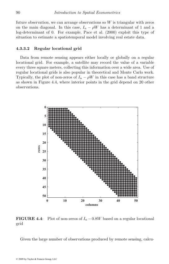
90 Introduction to Spatial Econometrics
future observation, we can arrange observations so W is triangular with zeroson the main diagonal. In this case, In − ρW has a determinant of 1 and alog-determinant of 0. For example, Pace et al. (2000) exploit this type ofsituation to estimate a spatiotemporal model involving real estate data.
4.3.3.2 Regular locational grid
Data from remote sensing appears either locally or globally on a regularlocational grid. For example, a satellite may record the value of a variableevery three square meters, collecting this information over a wide area. Use ofregular locational grids is also popular in theoretical and Monte Carlo work.Typically, the plot of non-zeros of In − ρW in this case has a band structureas shown in Figure 4.4, where interior points in the grid depend on 20 otherobservations.
0 10 20 30 40 50
0
5
10
15
20
25
30
35
40
45
50
columns
row
s
FIGURE 4.4: Plot of non-zeros of In−0.8W based on a regular locationalgrid
Given the large number of observations produced by remote sensing, calcu-
© 2009 by Taylor & Francis Group, LLC
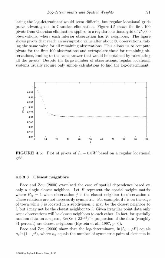
Log-determinants and Spatial Weights 91
lating the log-determinant would seem difficult, but regular locational gridsprove advantageous in Gaussian elimination. Figure 4.5 shows the first 100pivots from Gaussian elimination applied to a regular locational grid of 25, 000observations, where each interior observation has 20 neighbors. The figureshows pivots that reach an asymptotic value after about 30 observations, tak-ing the same value for all remaining observations. This allows us to computepivots for the first 100 observations and extrapolate these for remaining ob-servations, leading to the same answer that would be obtained by calculatingall the pivots. Despite the large number of observations, regular locationalsystems usually require only simple calculations to find the log-determinant.
0 10 20 30 40 50 60 70 80 90 1000.95
0.955
0.96
0.965
0.97
0.975
0.98
0.985
0.99
0.995
1
i
Piv
ot i
FIGURE 4.5: Plot of pivots of In − 0.8W based on a regular locationalgrid
4.3.3.3 Closest neighbors
Pace and Zou (2000) examined the case of spatial dependence based ononly a single closest neighbor. Let B represent the spatial weight matrixwhere Bij = 1 when observation j is the closest neighbor to observation i.These relations are not necessarily symmetric. For example, if i is on the edgeof town while j is located in a subdivision, j may be the closest neighbor toi, but i may not be the closest neighbor to j. Given irregular point data onlysome observations will be closest neighbors to each other. In fact, for spatiallyrandom data on a square, 3π(8π + 331/2)−1 proportion of the data (roughly31 percent) are closest neighbors (Epstein et al., 1997, p. 6).
Pace and Zou (2000) show that the log-determinant, ln |In − ρB| equalsns ln(1 − ρ2), where ns equals the number of symmetric pairs of elements in
© 2009 by Taylor & Francis Group, LLC
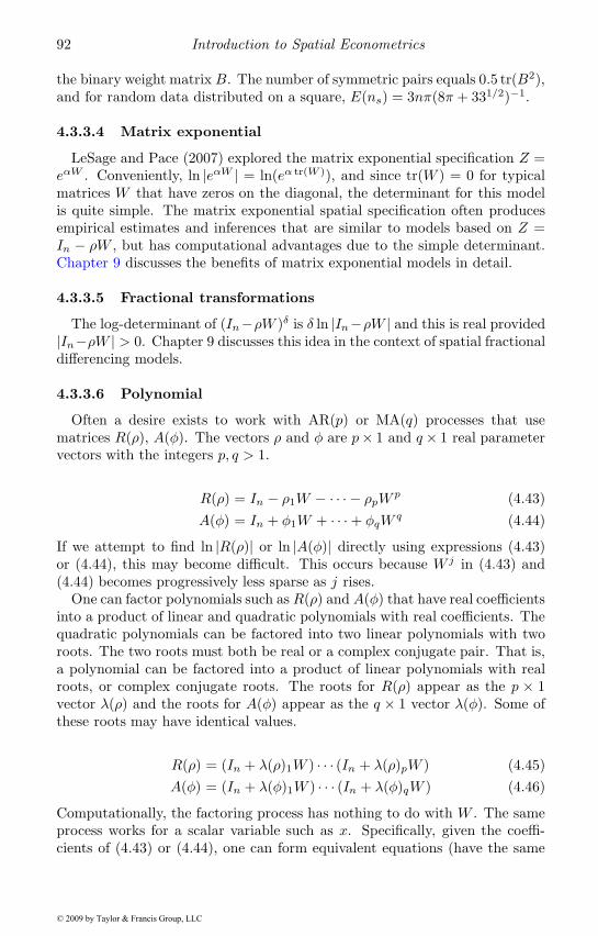
92 Introduction to Spatial Econometrics
the binary weight matrix B. The number of symmetric pairs equals 0.5 tr(B2),and for random data distributed on a square, E(ns) = 3nπ(8π + 331/2)−1.
4.3.3.4 Matrix exponential
LeSage and Pace (2007) explored the matrix exponential specification Z =eαW . Conveniently, ln |eαW | = ln(eα tr(W )), and since tr(W ) = 0 for typicalmatrices W that have zeros on the diagonal, the determinant for this modelis quite simple. The matrix exponential spatial specification often producesempirical estimates and inferences that are similar to models based on Z =In − ρW , but has computational advantages due to the simple determinant.Chapter 9 discusses the benefits of matrix exponential models in detail.
4.3.3.5 Fractional transformations
The log-determinant of (In−ρW )δ is δ ln |In−ρW | and this is real provided|In−ρW | > 0. Chapter 9 discusses this idea in the context of spatial fractionaldifferencing models.
4.3.3.6 Polynomial
Often a desire exists to work with AR(p) or MA(q) processes that usematrices R(ρ), A(φ). The vectors ρ and φ are p× 1 and q × 1 real parametervectors with the integers p, q > 1.
R(ρ) = In − ρ1W − · · · − ρpWp (4.43)
A(φ) = In + φ1W + · · · + φqWq (4.44)
If we attempt to find ln |R(ρ)| or ln |A(φ)| directly using expressions (4.43)or (4.44), this may become difficult. This occurs because W j in (4.43) and(4.44) becomes progressively less sparse as j rises.
One can factor polynomials such as R(ρ) and A(φ) that have real coefficientsinto a product of linear and quadratic polynomials with real coefficients. Thequadratic polynomials can be factored into two linear polynomials with tworoots. The two roots must both be real or a complex conjugate pair. That is,a polynomial can be factored into a product of linear polynomials with realroots, or complex conjugate roots. The roots for R(ρ) appear as the p × 1vector λ(ρ) and the roots for A(φ) appear as the q × 1 vector λ(φ). Some ofthese roots may have identical values.
R(ρ) = (In + λ(ρ)1W ) · · · (In + λ(ρ)pW ) (4.45)A(φ) = (In + λ(φ)1W ) · · · (In + λ(φ)qW ) (4.46)
Computationally, the factoring process has nothing to do with W . The sameprocess works for a scalar variable such as x. Specifically, given the coeffi-cients of (4.43) or (4.44), one can form equivalent equations (have the same
© 2009 by Taylor & Francis Group, LLC
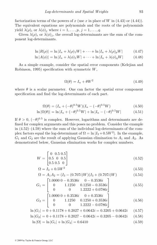
Log-determinants and Spatial Weights 93
factorization terms of the powers of x (use x in place of W in (4.43) or (4.44)).The equivalent equations are polynomials and the roots of the polynomialsyield λ(ρ)i or λ(φ)j where i = 1, . . . , p, j = 1, . . . , q.
Given λ(ρ)i or λ(φ)j , the overall log-determinants are the sum of the com-ponent log-determinants.
ln |R(ρ)| = ln |In + λ(ρ)1W | + · · · + ln |In + λ(ρ)pW | (4.47)ln |A(φ)| = ln |In + λ(φ)1W | + · · · + ln |In + λ(φ)qW | (4.48)
As a simple example, consider the spatial error components (Kelejian andRobinson, 1995) specification with symmetric W ,
Ω(θ) = In + θW 2 (4.49)
where θ is a scalar parameter. One can factor the spatial error componentspecification and find the log-determinants of each part.
Ω(θ) = (In + (−θ)0.5W )(In − (−θ)0.5W ) (4.50)ln |Ω(θ)| = ln |In + (−θ)0.5W | + ln |In − (−θ)0.5W | (4.51)
If θ > 0, (−θ)0.5 is complex. However, logarithms and determinants are de-fined for complex arguments and this poses no problem. Consider the examplein (4.52)–(4.59) where the sum of the individual log-determinants of the com-plex factors equal the log-determinant of Ω = ln |I3 +0.5W 2|. In the example,G1 and G2 are the result of applying Gaussian elimination to A1 and A2. Asdemonstrated below, Gaussian elimination works for complex numbers.
W =
⎡⎣ 0 0.5 0.50.5 0 0.50.5 0.5 0
⎤⎦ (4.52)
Ω = I3 + 0.5W 2 (4.53)Ω = A1A2 = (I3 − (0.707i)W )(I3 + (0.707i)W ) (4.54)
G1 =
⎡⎣1.0000 0 − 0.3536i 0 − 0.3536i0 1.1250 0.1250− 0.3536i0 0 1.2222 + 0.0786i
⎤⎦ (4.55)
G2 =
⎡⎣1.0000 0 + 0.3536i 0 + 0.3536i0 1.1250 0.1250 + 0.3536i0 0 1.2222− 0.0786i
⎤⎦ (4.56)
ln |G1| = 0 + 0.1178 + 0.2027 + 0.0642i = 0.3205 + 0.0642i (4.57)ln |G2| = 0 + 0.1178 + 0.2027− 0.0642i = 0.3205− 0.0642i (4.58)ln |Ω| = ln |G1| + ln |G2| = 0.6410 (4.59)
© 2009 by Taylor & Francis Group, LLC
94 Introduction to Spatial Econometrics
To summarize, the coefficients of the AR or MA in (4.43) or (4.44) canbe factored into products of simple linear factors as in (4.45) or (4.46). Thefactorization process works with the simpler scalar polynomial and requiresalmost no time to compute. These factors take the form In + λW where λmay be real or complex.
One can still form a table of log-determinants and interpolate over this toaccelerate calculations. However, now the table relating log-determinants toarguments is three-dimensional. Specifically, the table contains a real partargument, complex part argument, and the log-determinant. Using this tech-nique we can rely on a single table to store all log-determinants for differentfactors in the polynomial. Consequently, the log-determinant of polynomialfunctions of weight matrices has almost the same computational cost as thelog-determinant of the linear function In − ρW .
We discussed SARMA models in Chapter 3 and we will discuss fitting mul-tiple weight matrices in Chapter 5. The determinant table approach presentedabove could allow higher-order SARMA models to be fitted with large datasets. This approach could be used in conjunction with MCMC to deal withpotential local optima that can arise in these models.
4.3.3.7 Kronecker products
Spatial simultaneous equations, spatial vector autoregressions, and origin-destination flow data may require finding ln |Inm−Anm| where Anm = (Λ⊗W )and Λ is a m ×m matrix. Fortunately, the structure of Kronecker productsgreatly facilitates calculation of the log-determinant. Using the Taylor seriesexpansion of the log-determinant produces (4.60) and (4.61).
ln |Inm −Anm| = −∞∑i=1
tr(Ainm)i
(4.60)
ln |Inm −Anm| = −∞∑i=1
tr(Λi) tr(W i)i
(4.61)
The use of a trace estimator discussed in Section 4.4.1.2 enables efficientcalculation of traces for the powers of W . In the typical case where m issubstantially less than n, exact computation of tr(Λi) requires little time.Therefore, what appears to be an nm×nm problem reduces to separate n×nand m×m problems.
A related point is that eigenvalues of Anm equal the nm cross-productsbetween the eigenvalues of W and Λ, which facilitate calculating the log-determinant. The computational demands of calculating eigenvalues limitsthis technique to problems involving small or moderate n.
Models used for origin-destination flow data discussed in Chapter 8 provideanother example where the log-determinant involves Kronecker products of
© 2009 by Taylor & Francis Group, LLC
Log-determinants and Spatial Weights 95
matrices. LeSage and Pace (2008) consider a model involving spatial depen-dence among N = n2 flows, resulting in the log-determinant expression in(4.62).
B = IN − ρ1(In ⊗W ) − ρ2(W ⊗ In) − ρ3(W ⊗W ) (4.62)B = IN −A (4.63)
They proceed by finding tr(Aj) where A appears in (4.63). While findingthe trace of a n2 × n2 matrix seems difficult, in reality the log-determinantof B simply involves weighted traces of the powers of W . To see this, con-sider that any power of A greater than 1 will result in products and cross-products involving the components of A. The cross-product (In ⊗W ) and(W ⊗W ) can be expressed as (W ⊗W 2) using the Kronecker mixed productrule. This expression has a trace of tr(W ) tr(W 2) = 0, since tr(W ) = 0, andthis is a scalar. Because each product and cross-product has a form involvingtraces of powers of W , a pre-computed table of these traces facilitates re-weighting these to arrive at an approximation of the overall log-determinant.For any combination of ρ1, ρ2, and ρ3, the products and cross-products arealso scalars, and these represent coefficients associated with the traces. Multi-plying the pre-computed traces by these coefficients yields an estimate of thelog-determinant. Chapter 8 discusses spatial modeling of flow data in detail.
4.3.3.8 Multiple and parameterized W
We have already discussed models where Z = In−ρ1W1−ρ2W2, andW1 andW2 are not functionally related (Lacombe, 2004). More complicated modelscan be constructed that rely on functions of functionally unrelated multipleweight matrices. If both W1 and W2 are row-stochastic matrices, ρ1 +ρ2 < 1,and ρ1, ρ2 ≥ 0, Z is strictly diagonally dominant and thus non-singular. Thelog-determinant as a function of these parameters is smooth when ρ1 +ρ2 < 1and ρ1, ρ2 ≥ 0, since the first and second derivatives are continuous. Thisallows tabulation and interpolation of the log-determinants to produce a finergrid over values of ρ1, ρ2. However, in this case of two log-determinants, thetable now has two arguments (ρ1 and ρ2) which will require more time tocompute as well as more storage space. A natural extension of this appliesto three or more weight matrices. However, the logistical, computational andstorage difficulties increase with additional weight matrices and parameters.
In many cases, the individual weight matrices exhibit some natural orderor smoothness conditions. For example, consider Z = In − ρ1W1 − ρ2W2 −ρ3W3, where W1,W2,W3 represent first-, second- and third-nearest neighbormatrices. In this case, one might impose a monotonic restriction on ρ1, ρ2,and ρ3, using the restriction: ρi = ργi(γ + γ2 + γ3)−1. This converts amultiple parameter problem to a simpler two parameter problem involvingonly ρ and γ, which can easily be tabulated. Possible functions that could
© 2009 by Taylor & Francis Group, LLC
96 Introduction to Spatial Econometrics
serve as smoothing restrictions include polynomials (in the spirit of Almondistributed lags), geometric decay, exponential decay, and so on.
4.3.3.9 Local W
Suppose we wish to examine a more local system. For example, given a clus-ter of homes at the city center we begin adding observations on progressivelymore distant homes. How do these new observations affect the dependenceas measured by the log-determinant? Suppose Z = I3 − 0.8W where W isthe same as in (4.52). In numerical terms, Z appears in (4.65) and Gaussianelimination of Z, labeled G, appears in (4.66).
Z = I3 − 0.8W (4.64)
Z =
⎡⎣ 1.0000 −0.4000 −0.4000−0.4000 1.0000 −0.4000−0.4000 −0.4000 1.0000
⎤⎦ (4.65)
G =
⎡⎣1.0000 −0.4000 −0.40000 0.8400 −0.56000 0 0.4667
⎤⎦ (4.66)
The determinant of Z11 is 1 and this matches the first pivot of G. Thedeterminant of the first two rows and columns of Z is 1 − (−0.4)2 = 0.84,and this matches the product of the first and second pivots of G. Finally,using the formula for the determinant of Z yields a value of 0.3920, and thismatches the product of all three pivots of G. Consequently, a bonus arisingfrom Gaussian elimination is the sequence of log-determinants that result fromadding additional observations to the system. Pace and LeSage (2003a) usethis feature of log-determinants to estimate a sequence of SDM local estimatesaround each observation in the sample.
4.4 Monte Carlo approximation of the log-determinant
The log-determinant equals the trace of the matrix logarithm as shown in(4.67). In turn the matrix logarithm has a simple infinite series expansion interms of the powers of W as shown in (4.68). Since the trace operation islinear (tr(A + B) = tr(A) + tr(B)), the log-determinant is a weighted seriesof traces of the powers of W as shown in (4.69).
© 2009 by Taylor & Francis Group, LLC
Log-determinants and Spatial Weights 97
ln |In − ρW | = tr (ln(In − ρW )) (4.67)
ln(In − ρW ) = −∞∑i=1
ρiW i
i(4.68)
ln |In − ρW | = −∞∑i=1
ρi tr(W i)i
(4.69)
Since the logarithm is defined over the complex plane (except for ln(0)), (4.69)still holds for non-symmetric W that may have complex eigenvalues or forcomplex ρ.
One can partition the infinite series into a finite, lower order series and aremainder denoted by R composed of higher-order infinite expressions such as(4.70) and (4.71). Martin (1993) initially proposed this approach to dealingwith the log-determinant.
ln |In − ρW | = −o∑i=1
ρi tr(W i)i
−∞∑
i=o+1
ρi tr(W i)i
(4.70)
ln |In − ρW | = −o∑i=1
ρi tr(W i)i
−R (4.71)
If R is small, one can approximate the log-determinant through a finite,lower-order series as in (4.72).
ln |In − ρW | ≈ −o∑i=1
ρi tr(W i)i
(4.72)
From a computational perspective, forming W j and then taking the traceis costly and inefficient having an operational count of up to O(n3) when W j
is dense.
Fortunately, other methods exist for estimating traces. For example, let urepresent a 2× 1 vector of independent unit normals and A a 2× 2 matrix asin (4.73) and (4.74). The expectation of the quadratic form u′Au equals tr(A)since u2
i follows a χ2 distribution with one degree of freedom. Of course, thishas an expectation equal to 1, whereas E(uiuj) = 0 for i �= j as in (4.75) to(4.78).
© 2009 by Taylor & Francis Group, LLC
98 Introduction to Spatial Econometrics
A =[a bc d
], u =
[u1
u2
](4.73)
u′Au = u21a+ u2
2d+ u1u2(b+ c) (4.74)E(u′Au) = E(u2
1)a+ E(u22)d+ E(u1u2)(b + c) (4.75)
E(u2i ) = 1 (4.76)
E(uiuj) = 0 i �= j (4.77)E(u′Au) = a+ d = tr(A) (4.78)
Let T (i)(j) represent the estimate of tr(W i) using the jth n by 1 random unit
normal vector u(j) as shown in (4.79). For convenience, we will term u(j) thejth seed, and Girard (1989) proposed normal seeds in estimating traces.2
T(i)(j) = u′(j)W
iu(j) (4.79)
Given the estimated tr(W i) which equals T (i)(j) , one could use this to form
an estimate of the log-determinant based on the estimated trace.3
ln |In − ρW |(j) ≈ −o∑i=1
ρiT(i)(j)
i(4.80)
Calculating ln |In − ρW |(j) across m independent u(j) and averaging theresults can improve the accuracy of the log-determinant estimate. Each ofthe ln |In − ρW |(j) are independent, so the variance of the averaged estimateis 1/m times the variance of a single estimate ln |In − ρW |(j).
ln |In − ρW | ≈(
1m
) m∑j=1
ln |In − ρW |(j) (4.81)
Also, calculating m log-determinant estimates ln |In − ρW |(j) allows esti-mating the variance of the log-determinant, and therefore confidence intervalsassociated with the averaged log-determinant estimate.
From a computational perspective, the algorithm begins by picking the seedu(j), initializing the loop by setting z(1) to u(j), and by calculating a matrix-vector product z(t + 1) = Wz(t) as well as T (i)
(j) = z(1)′z(t + 1) over a loop
2Barry and Pace (1999) rediscovered the normal seed without the benefit of the work ofGirard (1989) and gave different proofs of the performance of normal seeds in estimatingthe trace.3Barry and Pace (1999) actually used T(j) = [n(u′
(j)u(j))
−1]T(j). This has slightly lower
variability than T(j), but T(j) has the advantage of simplicity.
© 2009 by Taylor & Francis Group, LLC
Log-determinants and Spatial Weights 99
from t = 1, . . . , o. This can be repeated m times to improve the precision ofthe trace estimates and thus the log-determinant estimates by averaging overT
(i)(j) for j = 1, . . . ,m to yield T (i). In addition, having the T (i)
(j) allows easycalculation of confidence intervals for the estimated log-determinant. Thealgorithm has computational complexity O(nmo) and therefore is linear in n.
Given the estimated T (i), an outstanding advantage of the algorithm is thatcomputation of ln |In−ρW | for any ρ requires almost no time. Let a representan o × 1 vector so that ai = −T (i)/i and let b =
[ρ, ρ2, . . . , ρo
]′. Thelog-determinant estimate for a particular ρ is just a′b, a simple dot productbetween two vectors of length o where o might be 100. Therefore, updatingthe estimate of the log-determinant for a new value of ρ is virtually costless.
A few refinements boost the computational speed and accuracy. First, onecan employ symmetry to reduce the work by half. For symmetric W , letv = W iu and therefore v′v = u′W 2iu which estimates the trace of (W 2i).Second, the lower-order exact moments are either known or easily computed,and using these can materially reduce the approximation error. For example,tr(W ) = 0 by construction whereas tr(W p+q) = ι′n((W
p)′�W q)ιn. Therefore,tr(W 2) for a symmetric matrix is the sum of squares of all the elements inW . It does not take long to compute these exact traces. For example, usinga contiguity-based W where n = 1, 024, 000, it takes 0.43 seconds to computeW 2 and 6.3 seconds to find tr(W 4). The computational requirements of theexact traces in general rise at a faster than linear rate, but computing thelower order exact traces is quite feasible for sparseW . Third, one can improvethe choice of seeds u(j) by rejecting “bad” seeds where “bad” in this contextmeans that the estimated moments differ significantly from the known lowerorder exact moments (Zhang et al., 2008).
This raises the issue of seed choice. Alternatives to the normal seed pro-posed by Girard (1989) include using n independent draws of −1 and 1 withequal probability as a seed (Hutchinson, 1990). Also, a seed where the kthelement of u(j) equals 1 and the other elements equal 0 will yield the diagonalelement of W i
kk. Selecting k randomly over [1, n] for m samples and averagingthese samples yields an estimate of n−1 tr(W i). For all of these approaches,the use of m independent realizations naturally facilitates parallel processing.All seed choices work well for moderate m, but we have found that the normalseed performs better for very small m (including m = 1).
Ideally, approximations should provide a means to assess accuracy whichmight be measured in terms of the impact on variables of interest in appliedproblems. One approach to this is to consider how independent estimatesof the log-determinant affect the estimated parameter ρ in the autoregres-sive model. We take this approach in Section 4.4.1. Since one can rapidlysolve for the spatial dependence parameter estimate given the log-determinantfunction, we could use m independent estimates of the log-determinant. Thiswould lead to m estimates for ρ, and variation in these estimates would serveas a guide to the approximation accuracy. If the variation is small relative to
© 2009 by Taylor & Francis Group, LLC
100 Introduction to Spatial Econometrics
the standard error of the parameter estimate, this indicates that the approx-imation error does not materially degrade parameter estimation.
4.4.1 Sensitivity of ρ estimates to approximation
Useful approximations contain errors that do not materially affect the re-sults. In Section 4.4.1.1, we explore the dispersion in the estimated valueof ρ that arises from a log-determinant approximation using a Monte Carloexperiment. We show that the approximation is very accurate in that it doesnot materially affect the estimate or inference regarding the parameter ρ.Section 4.4.1.2 and Section 4.4.1.3 provide detailed Monte Carlo experimentsthat explore the nature of the approximation error that leads to accuracy ofthe Monte Carlo log-determinant approximation of Barry and Pace (1999) inapplied practice.
4.4.1.1 Error in ρ using individual MC log-determinant estimates
To assess the accuracy of the Monte Carlo log-determinant estimator, weconducted an experiment with sample sizes n ranging from 1, 000 to 1, 024, 000.For each sample size we generated a random set of points, calculated a con-tiguity weight matrix Wn, and simulated the dependent variable using yn =(In − 0.75Wn)−1(Xβ + ε). The matrix X contained an intercept as well asa vector of standard normal random deviates, and β was set to ι2. An iidnormal vector was used for ε with a standard deviation of 0.25. For each ynwe calculated 100 separate estimated log-determinants using the Barry andPace (1999) Monte Carlo approximation.
These estimated log-determinants did not involve averaging across multipleestimated log-determinants as is typically done in application of the Barryand Pace (1999) approach. The reported results were based on a single nor-mal vector (normal seed) used in the Monte Carlo log-determinant estimator.Using a single vector to estimate the log-determinant is seemingly quite ex-treme, since Barry and Pace (1999) recommend use of 30 to 50 such vectorsin their statistical approximation. To gauge performance of the individuallog-determinant estimates, we also averaged over all 100 log-determinant es-timates to produce a more accurate estimate.
Table 4.2 shows the results from using an average of all log-determinant es-timates versus 100 separate estimates of the log-determinant where each esti-mate corresponds to a different normal seed. The estimated log-determinantsused four exact lowest-order moments and 100 total moments.
Rather surprisingly, the estimated ρ was not sensitive to numerical approx-imation error present in the individual MC log-determinant estimates. Across100 trials of the individual MC log-determinant estimates, the estimated de-pendence parameter varied over a very small range that declined with n. Theaverage estimated dependence parameter was very close to the actual valueof 0.75. For example, when n = 1, 024, 000, the average estimated ρ across
© 2009 by Taylor & Francis Group, LLC
Log-determinants and Spatial Weights 101
the 100 separate log-determinants was 0.749404, and the range between thelargest and smallest estimate was only 0.000052. Using an average of the 100log-determinants produces the same estimate for ρ to six decimal places. Ittook only 23.7 seconds, on average, to estimate the log-determinant of the1, 024, 000× 1, 024, 000 matrix.
TABLE 4.2: Estimates of ρ based on aggregate vs. individual MClog-determinant estimates
n ρln|z|i mean ρln|z|i range ρln|z|i Seconds per ln-det
1, 000 0.762549 0.762550 0.002119 0.0052812, 000 0.752098 0.752099 0.001359 0.0075934, 000 0.751474 0.751475 0.000873 0.0135048, 000 0.752152 0.752152 0.000748 0.032123
16, 000 0.747034 0.747034 0.000485 0.07008632, 000 0.748673 0.748673 0.000339 0.19720064, 000 0.750238 0.750238 0.000224 0.453033
128, 000 0.750622 0.750622 0.000147 1.153523256, 000 0.749766 0.749766 0.000122 3.917425512, 000 0.750144 0.750144 0.000068 10.498189
1, 024, 000 0.749404 0.749404 0.000052 23.710256
4.4.1.2 Trace estimation accuracy
The accuracy of the Monte Carlo estimates for the log-determinant raisethe question of why it works so well. Either the procedure estimates traces ex-tremely well, the shape of the log-likelihood is not sensitive to small variationsin the log-determinant, or some combination of both factors is at work. Inthis section, we investigate the accuracy of the trace estimates with an exper-iment. We estimate n−1 tr(W 2) which we denote tr using a contiguity weightmatrix and compare these estimates to the exact trace tr = n−1 tr(W 2). Ta-ble 4.3 shows the results from this experiment for varying n. As expected, theMonte Carlo estimate of the trace appears more or less unbiased having smallaverage errors that vary in sign across n. In addition, the standard deviationand ranges of the estimated traces are small. For sample sizes of 16, 000 andabove, we see a difference of less than 0.01 between the largest and smallestestimated traces across the 100 trials. Again, these results are for single tri-als or iterations. Aggregating the different trials or iterations would furtherimprove the performance.
These results conform to the theoretical investigations of Girard (1989, p.5) as well as Barry and Pace (1999, p. 52) where σ2(T (i)
(j)) = κn−1 and κ is aconstant.
© 2009 by Taylor & Francis Group, LLC
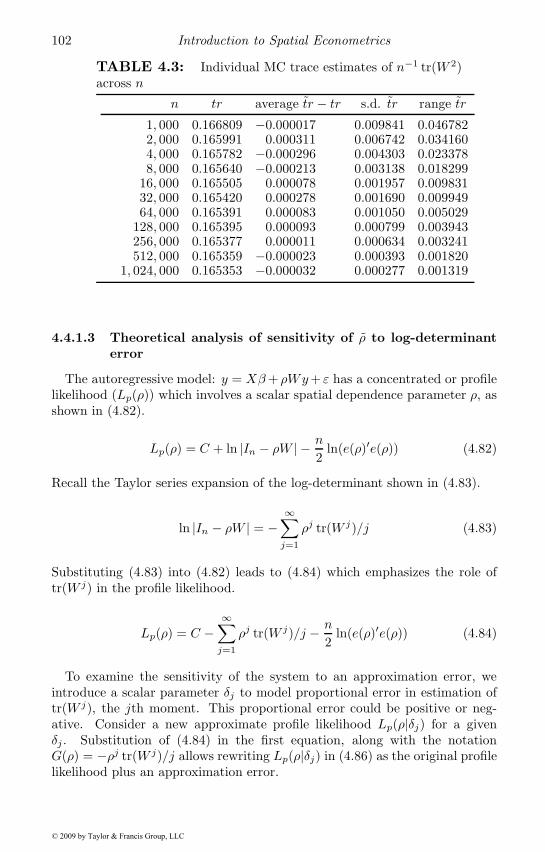
102 Introduction to Spatial Econometrics
TABLE 4.3: Individual MC trace estimates of n−1 tr(W 2)across n
n tr average tr − tr s.d. tr range tr
1, 000 0.166809 −0.000017 0.009841 0.0467822, 000 0.165991 0.000311 0.006742 0.0341604, 000 0.165782 −0.000296 0.004303 0.0233788, 000 0.165640 −0.000213 0.003138 0.018299
16, 000 0.165505 0.000078 0.001957 0.00983132, 000 0.165420 0.000278 0.001690 0.00994964, 000 0.165391 0.000083 0.001050 0.005029
128, 000 0.165395 0.000093 0.000799 0.003943256, 000 0.165377 0.000011 0.000634 0.003241512, 000 0.165359 −0.000023 0.000393 0.001820
1, 024, 000 0.165353 −0.000032 0.000277 0.001319
4.4.1.3 Theoretical analysis of sensitivity of ρ to log-determinanterror
The autoregressive model: y = Xβ+ ρWy+ ε has a concentrated or profilelikelihood (Lp(ρ)) which involves a scalar spatial dependence parameter ρ, asshown in (4.82).
Lp(ρ) = C + ln |In − ρW | − n
2ln(e(ρ)′e(ρ)) (4.82)
Recall the Taylor series expansion of the log-determinant shown in (4.83).
ln |In − ρW | = −∞∑j=1
ρj tr(W j)/j (4.83)
Substituting (4.83) into (4.82) leads to (4.84) which emphasizes the role oftr(W j) in the profile likelihood.
Lp(ρ) = C −∞∑j=1
ρj tr(W j)/j − n
2ln(e(ρ)′e(ρ)) (4.84)
To examine the sensitivity of the system to an approximation error, weintroduce a scalar parameter δj to model proportional error in estimation oftr(W j), the jth moment. This proportional error could be positive or neg-ative. Consider a new approximate profile likelihood Lp(ρ|δj) for a givenδj . Substitution of (4.84) in the first equation, along with the notationG(ρ) = −ρj tr(W j)/j allows rewriting Lp(ρ|δj) in (4.86) as the original profilelikelihood plus an approximation error.
© 2009 by Taylor & Francis Group, LLC
Log-determinants and Spatial Weights 103
Lp(ρ|δj) = C − δjρj tr(W j)/j −
∞∑j=1
ρj tr(W j)/j − n
2ln(e(ρ)′e(ρ))
Lp(ρ|δj) = −δjρj tr(W j)/j + Lp(ρ) (4.85)Lp(ρ|δj) = δjG(ρ) + Lp(ρ) (4.86)
We form the score function, Sp(ρ|δj) for a given δj .
Sp(ρ|δj) =dLp(ρ|δj)
dρ= δj
dG(ρ)dρ
+dLp(ρ)dρ
(4.87)
The score function set to 0 is the first-order condition for an optimum andthis forms an implicit function F .
F = Sp(ρ|δj) = 0 (4.88)
Given unimodality of the profile likelihood for this problem, a unique valueof ρ solves the implicit equation F = 0, but the solution depends upon theerror δj . We can examine the sensitivity of the dependence parameter ρ withrespect to the error δj using the implicit function theorem for two variables(which allows for total instead of partial derivatives) as shown in (4.89).
dρ
dδj= − dF
dδj/dF
dρ(4.89)
Taking the derivative of F with respect to δj yields (4.90).dF
dδj=dG(ρ)dρ
(4.90)
The derivative of F with respect to ρ yields (4.91).
dF
dρ= δj
d2G(ρ)dρ2
+d2Lp(ρ)dρ2
(4.91)
Using (4.89), (4.90), and (4.91) yields (4.92).
dρ
dδj= −
[δjd2G(ρ)dρ2
+d2Lp(ρ)dρ2
]−1dG(ρ)dρ
(4.92)
We now consider simplifying this expression, noting that the second deriva-tive of Lp(ρ) with respect to ρ is the Hessian H(ρ) (Davidson and MacKinnon,1993, p. 267-269).
d2Lp(ρ)dρ2
=dSp(ρ)dρ
= H(ρ) (4.93)
Given an estimated ρ, the estimated variance of ρ is σ2(ρ). Equation (4.94)expresses the well-known relation between the Hessian and the variance of
© 2009 by Taylor & Francis Group, LLC
104 Introduction to Spatial Econometrics
a parameter estimate for a univariate function such as our concentrated loglikelihood.
σ2(ρ) = −H(ρ)−1 (4.94)
Using (4.94) provides an additional simplification.
d2Lp(ρ)dρ2
= H(ρ) = −σ−2(ρ) (4.95)
Taking (4.95) and (4.92) in conjunction with dG(ρ)/dρ = −ρj−1 tr(W j), eval-uated around the point of δj = 0, leads to (4.96).
dρ
dδj
∣∣∣∣∣(δj=0)
= −σ2(ρ)ρj−1 tr(W j) (4.96)
The fact that dρ/dδj < 0 for positive ρ makes intuitive sense. Positive δjresults in a more severe log-determinant penalty, and this should depress ρ.Turning to the relative magnitudes of these variables, the estimated variance(σ2(ρ)) of ρ decreases with n, while tr(W j) rises with n. This suggests theproduct of these two variables should not greatly vary with n.
Putting this in differential form in (4.97), we note that from the startingpoint of δj = 0, dδj equals the proportional error in the jth moment, whichcould be negative or positive. In other words, going to δ
(1)j from δ
(0)j = 0
means that dδj , the change in the variable, equals δ(1)j .
dρ =dρ
dδjδj (4.97)
However, as was demonstrated, δj , the proportional error in the jth momenttends to decrease with n, so the overall numerical error associated with ρ tendsto decrease with n.
To examine the relative magnitudes of these terms in applied practice, weperformed a simple Monte Carlo experiment. A set of 2, 500 random pointswere generated and a contiguity weight matrix W was used to simulate: y =(In−0.75W )−1(Xβ+ε), whereX contains an intercept column plus a standardnormal vector. The parameter β was set equal to ι2, and an iid normal εhaving a standard deviation of 0.25 was used. Exact traces for orders 1 to100 were calculated using a set of 1, 000 instances of y, with the exception oftr(W 6). For this single exception, we added a proportional error equal to 0.01,and calculated the theoretical as well as empirical change in ρ in response toa one percent error in tr(W 6).
On average, the empirical change was −0.629453 · 10−5 while the predictedchange was −0.630461·10−5. The difference between empirical and theoreticalerrors was not statistically significant. Given that δj = 0.01, dρ/dδj approx-imately equals −0.00063 for this case. Consequently, ρ is not very sensitive
© 2009 by Taylor & Francis Group, LLC
Log-determinants and Spatial Weights 105
to proportional error in one of the traces. A similar experiment using othervalues of n demonstrated that this derivative does not vary materially withn.
To summarize, the sensitivity of ρ to approximation errors for the log-determinant in a single trace depends on: the variance associated with theestimate of ρ, true value of the trace, true value of ρ, and the proportionalerror in estimating the trace. The combination of the first three factors shouldhave a value which does not vary greatly with n. This is because the tracerises linearly with n (all else equal) and the variance declines linearly withn. However, the proportional error in estimating the trace declines with n.Specifically, σ2(T (i)
(j)) = κn−1 where κ is a constant (Barry and Pace, 1999,p. 52). Consequently, the sensitivity of ρ to log-determinant error decreaseswith sample size.
4.5 Chebyshev approximation
Taylor series approximations provide good results around the point of ex-pansion (ρ = 0 in the previous section). In contrast, Chebyshev approxi-mations minimize errors over a range, attempting to minimize the maximumerror over the entire interval. Pace and LeSage (2004) applied the Chebyshevapproximation technique to the log-determinant problem.
The basic idea is to approximate the matrix function ln(In−ρW ) using theChebyshev polynomials as well as Chebyshev coefficients, and use the traceof these to produce an estimate of the log-determinant. Following Press etal. (1996), let cj represent the Chebyshev coefficients (4.98) associated withthe function ln(1 − ρx), where x is real and lies on [−1, 1]. We furthermoreassume W is symmetric with a maximum eigenvalue of 1 and we restrict ρ to(−1, 1). The coefficients in (4.98) depend on the evaluation points x in (4.99)as well as the specific scalar function f(x) under consideration. In this case,the function of interest is ln(1 − ρx) as shown in (4.100), and we note thatthe desired matrix function inherits the same coefficients.
cj (ρ) =2
q + 1
q+1∑k=1
f (xk) cos
(π (j − 1)
(k − 1
2
)q + 1
)(4.98)
xk = cos
(π(k − 1
2
)q + 1
)(4.99)
f(x) = ln(1 − ρx) (4.100)
Given the Chebyshev polynomials in (4.102)–(4.107) and the coefficients in
© 2009 by Taylor & Francis Group, LLC
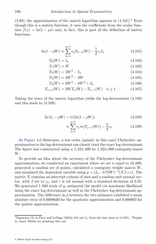
106 Introduction to Spatial Econometrics
(4.98), the approximation of the matrix logarithm appears in (4.101).4 Eventhough this is a matrix function, it uses the coefficients from the scalar func-tion f(x) = ln(1 − ρx) and, in fact, this is part of the definition of matrixfunctions.
ln(1 − ρW ) ≈q+1∑k=1
ckTk−1(W ) − 12c1In (4.101)
T0(W ) = In (4.102)T1(W ) = W (4.103)T2(W ) = 2W 2 − In (4.104)T3(W ) = 4W 3 − 3W (4.105)T4(W ) = 8W 4 − 8W 2 + In (4.106)
Tn+1(W ) = 2WTn(W ) − Tn−1(W ) n ≥ 1 (4.107)
Taking the trace of the matrix logarithm yields the log-determinant (4.108)and this leads to (4.109).
ln |In − ρW | = tr(ln(1 − ρW )) (4.108)
≈q+1∑j=1
cj tr(Tj−1(W )) − n
2c1 (4.109)
As Figure 4.6 illustrates, a low-order (quintic in this case) Chebyshev ap-proximation to the log-determinant can closely tract the exact log-determinant.The figure was constructed using a 1, 024, 000 by 1, 024, 000 contiguity-basedW .
To provide an idea about the accuracy of the Chebyshev log-determinantapproximation, we conducted an experiment where we set n equal to 10, 000,generated a random set of points, calculated a contiguity weight matrix W ,and simulated the dependent variable using y = (In−0.75W )−1(Xβ+ε). Thematrix X contains an intercept column of ones and a random unit normal vec-tor, with β set to ι2, and ε is iid normal with a standard deviation of 0.25.We generated 1, 000 trials of y, estimated the model via maximum likelihoodusing the exact log-determinant as well as the Chebyshev log-determinant ap-proximation. The difference in ρ between the two estimates exhibited a meanabsolute error of 0.0008630 for the quadratic approximation and 0.000002 forthe quintic approximation.
4Equation (3) in Pace and LeSage (2004) left out In from the last term in (4.101). Thanksto Janet Walde for pointing this out.
© 2009 by Taylor & Francis Group, LLC
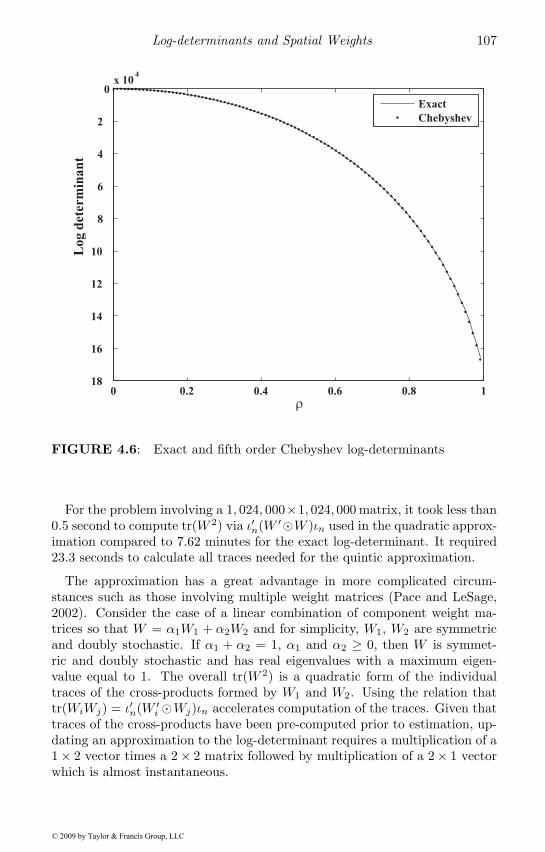
Log-determinants and Spatial Weights 107
0 0.2 0.4 0.6 0.8 118
16
14
12
10
8
6
4
2
0x 10
4
ρ
Lo
g d
eter
min
an
t
Exact
Chebyshev
FIGURE 4.6: Exact and fifth order Chebyshev log-determinants
For the problem involving a 1, 024, 000×1, 024, 000 matrix, it took less than0.5 second to compute tr(W 2) via ι′n(W
′�W )ιn used in the quadratic approx-imation compared to 7.62 minutes for the exact log-determinant. It required23.3 seconds to calculate all traces needed for the quintic approximation.
The approximation has a great advantage in more complicated circum-stances such as those involving multiple weight matrices (Pace and LeSage,2002). Consider the case of a linear combination of component weight ma-trices so that W = α1W1 + α2W2 and for simplicity, W1, W2 are symmetricand doubly stochastic. If α1 + α2 = 1, α1 and α2 ≥ 0, then W is symmet-ric and doubly stochastic and has real eigenvalues with a maximum eigen-value equal to 1. The overall tr(W 2) is a quadratic form of the individualtraces of the cross-products formed by W1 and W2. Using the relation thattr(WiWj) = ι′n(W
′i �Wj)ιn accelerates computation of the traces. Given that
traces of the cross-products have been pre-computed prior to estimation, up-dating an approximation to the log-determinant requires a multiplication of a1 × 2 vector times a 2 × 2 matrix followed by multiplication of a 2× 1 vectorwhich is almost instantaneous.
© 2009 by Taylor & Francis Group, LLC
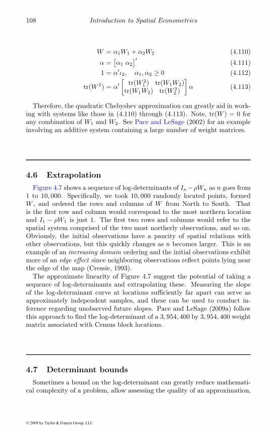
108 Introduction to Spatial Econometrics
W = α1W1 + α2W2 (4.110)
α =[α1 α2
]′(4.111)
1 = α′ι2, α1, α2 ≥ 0 (4.112)
tr(W 2) = α′[
tr(W 21 ) tr(W1W2)
tr(W1W2) tr(W 22 )
]α (4.113)
Therefore, the quadratic Chebyshev approximation can greatly aid in work-ing with systems like those in (4.110) through (4.113). Note, tr(W ) = 0 forany combination of W1 and W2. See Pace and LeSage (2002) for an exampleinvolving an additive system containing a large number of weight matrices.
4.6 Extrapolation
Figure 4.7 shows a sequence of log-determinants of In−ρWn as n goes from1 to 10, 000. Specifically, we took 10, 000 randomly located points, formedW , and ordered the rows and columns of W from North to South. Thatis the first row and column would correspond to the most northern locationand I1 − ρW1 is just 1. The first two rows and columns would refer to thespatial system comprised of the two most northerly observations, and so on.Obviously, the initial observations have a paucity of spatial relations withother observations, but this quickly changes as n becomes larger. This is anexample of an increasing domain ordering and the initial observations exhibitmore of an edge effect since neighboring observations reflect points lying nearthe edge of the map (Cressie, 1993).
The approximate linearity of Figure 4.7 suggest the potential of taking asequence of log-determinants and extrapolating these. Measuring the slopeof the log-determinant curve at locations sufficiently far apart can serve asapproximately independent samples, and these can be used to conduct in-ference regarding unobserved future slopes. Pace and LeSage (2009a) followthis approach to find the log-determinant of a 3, 954, 400 by 3, 954, 400 weightmatrix associated with Census block locations.
4.7 Determinant bounds
Sometimes a bound on the log-determinant can greatly reduce mathemati-cal complexity of a problem, allow assessing the quality of an approximation,
© 2009 by Taylor & Francis Group, LLC
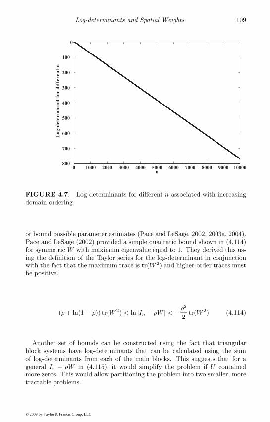
Log-determinants and Spatial Weights 109
0 1000 2000 3000 4000 5000 6000 7000 8000 9000 10000800
700
600
500
400
300
200
100
0
n
Lo
g-d
ete
rm
ina
nt
for
dif
feren
t n
FIGURE 4.7: Log-determinants for different n associated with increasingdomain ordering
or bound possible parameter estimates (Pace and LeSage, 2002, 2003a, 2004).Pace and LeSage (2002) provided a simple quadratic bound shown in (4.114)for symmetric W with maximum eigenvalue equal to 1. They derived this us-ing the definition of the Taylor series for the log-determinant in conjunctionwith the fact that the maximum trace is tr(W 2) and higher-order traces mustbe positive.
(ρ+ ln(1 − ρ)) tr(W 2) < ln |In − ρW | < −ρ2
2tr(W 2) (4.114)
Another set of bounds can be constructed using the fact that triangularblock systems have log-determinants that can be calculated using the sumof log-determinants from each of the main blocks. This suggests that for ageneral In − ρW in (4.115), it would simplify the problem if U containedmore zeros. This would allow partitioning the problem into two smaller, moretractable problems.
© 2009 by Taylor & Francis Group, LLC
110 Introduction to Spatial Econometrics
In − ρW = In − ρS − ρU (4.115)
S =[A B0 D
](4.116)
U =[
0 0C 0
](4.117)
The basic idea is that reducing the number of non-zero elements in U wouldlead to a positive bound on the log-determinant. In addition, subtracting ρtimes the elements in U from the main diagonal produces a lower bound onthe log-determinant. Let r = Uιn and Rii = ri for i = 1, . . . , n. In this case,one can bound the log-determinant as in (4.118).
ln |In − ρS| ≥ ln |In − ρW | ≥ ln |(In − ρR) − ρS| (4.118)
Skillful reordering of the observations can reduce the number and magnitudeof the elements of U . Pace and LeSage (2009c) use this approach to bound thelog-determinant of a 3, 954, 400×3, 954, 400 matrix. Since almost the same es-timate of dependence was obtained using the lower and upper log-determinantbounds, these proved as informative as the actual log-determinant. An ad-vantage of partitioning is the possibility of using parallel processing as well asreduced memory requirements.
Bounds may not yield a precise answer, but may yield a range of answers.Pace and LeSage (2003a) invoked likelihood dominance ideas to demonstratethat bounds could permit qualitative inferences concerning parameter esti-mates.
Various types of bounds can be combined with approximations such as theMonte Carlo log-determinant estimator or the Chebyshev approximation toprovide bounds on the approximations. For example, Barry and Pace (1999)bound the remainder term in the Taylor series approximation. For W withreal eigenvalues and a maximum eigenvalue of 1, tr(W 2j+1) < tr(W 2j) andtr(W 2(j+1)) < tr(W 2j). Consequently, the last even order estimated trace setsan upper bound on the remaining omitted traces. Using this sets up lowerand upper bounds on the omitted terms.
4.8 Inverses and other functions
Although the focus of this chapter has been on computing log-determinants,other functions involving the spatial weight matrixW deserve attention. First,(In − ρW )−1 often appears in various contexts. In the vast majority of thosecontexts, it appears in conjunction with a matrix or vector. For example,
© 2009 by Taylor & Francis Group, LLC
Log-determinants and Spatial Weights 111
v = (In − ρW )−1ε where ε is a n × 1 vector. In this case, it would be poorcomputational practice in terms of speed, memory requirements, and accuracyto compute (In − ρW )−1 and then multiply it by the vector ε. It would bebetter to solve the equation (In − ρW )v = ε for v.
One can do this using iterative techniques such as conjugate gradients orwith the LU or Cholesky decompositions. For example, suppose In − ρW =LU . In this case, LUv = ε which is identical to Lz = ε where z = Uv. Solvingthe triangular system Lz = ε for z, and then solving a second triangularsystem Uv = z for v yields the desired solution for v. Although it seems likemore work, it actually performs much better than the brute force approach,especially for sparse matrices. This is because (In − ρW )−1 is dense for aspatially connected system requiring n2 storage locations. In contrast, thesparse matrix has a much smaller storage footprint. The brute force approachis guaranteed to take O(n3) operations while solving the equation could takeas few as O(n) operations.
As an example, for n = 10, 000, forming (In− 0.75W )−1 and multiplying itby a 10, 000× 1 vector ε takes 86.0 seconds, while solving the equation takes0.071 seconds. It may seem that having the inverse available would save timewhen dealing with a new vector ε. Given the inverse, it takes 0.69 secondsto multiply the inverse and vector, and this is slower than solving the systemagain. However, for a given L and U , solving the system again with a newε takes 0.0056 seconds. From a memory perspective, it requires around 1.6gigabytes of memory to hold the 10, 000 × 10, 000 matrix whereas it takes4.62 megabytes for L and U . In addition, for symmetric W the Choleskydecomposition would take around half the memory and time required by theLU decomposition.
Chebyshev and Taylor series approximations can also aid in solving equa-tions. The function to be approximated is f(x) = 1/(1 − ρx). Given thecoefficients c0, . . . , cq of the series associated with the powers of W , the prob-lem in (4.119) reduces to (4.121) in which ε is multiplied by a power of W .Forming powers of W times the vector ε in the efficient manner described in(4.122) allows us to form u(1) = Wε, then Wu(1) = W 2ε. Therefore, calcu-lation of the q powers of the matrix times a vector just involves a set of qmatrix-vector operations.
v = (In − ρW )−1ε (4.119)v ≈ [
c0In + c1W + c2W2+, . . . ,+cqW q
]ε (4.120)
v ≈ c0ε+ c1Wε+, . . . ,+cqW qε (4.121)W jε = W (W j−1ε) (4.122)
To provide an indication of the performance of this approach, we simulateda spatial system with n = 10, 000, ρ = 0.75, and a vector of iid unit normalsfor ε. The correlation between the sixth-degree Chebyshev approximation of
© 2009 by Taylor & Francis Group, LLC
112 Introduction to Spatial Econometrics
v versus the exact version of v was equal to 0.999986. The time and storagerequirements of this approximation approach were de minimus.
Another problem which often arises is finding the diagonal of the inverse,diag((In− ρW )−1), as shown in (4.123). In practice, computing (In− ρW )−1
and finding the diagonal breaks down due to memory problems for data setssuch as the US Census tracts.
d = diag((In − ρW )−1) (4.123)d ≈ c0 diag(In) + c1 diag(W )+, . . . ,+cq diag(W q)d ≈ c0ιn + c10n + c2 diag(W 2)+, . . . ,+cq diag(W q)
The exact diagonals of the powers ofW can be efficiently computed via (4.124)
diag(WiWj) = (Wi �W ′j)ιn (4.124)
The diagonal of a matrix A can also be estimated via Monte Carlo as shownin (4.125)–(4.130).
A =[a bc d
], u =
[u1
u2
](4.125)
Au =[u1a+ u2b u1c+ u2d
]′ (4.126)
u� Au =[u2
1a+ u1u2b u2u1c+ u22d]′
(4.127)
E(u2i ) = 1 (4.128)
E(uiuj) = 0 i �= j (4.129)
E(u�Au) =[a d
]′ = diag(A) (4.130)
To do this efficiently, let v be an n×m matrix of iid unit normal deviates,where m is the number of vectors used in the approximation procedure. Webegin by setting the initial values v(0) = v. Monte Carlo estimates of thediagonals can be efficiently computed via (4.131)–(4.132).
v(j) = Wv(j−1) (4.131)
diag(W j) ≈ (v � v(j))ιmm
(4.132)
The term v � v(j) is an n ×m matrix where each column is an independentestimate of the diagonal. Post multiplying this by ιm sums across the m in-dependent estimates and dividing by m converts this into an average of them estimates. Relative to estimating the trace, m needs to be much larger foran accurate estimate the diagonal. Selection of m depends on the size of thediagonal elements and their variation. If memory is a problem, estimation
© 2009 by Taylor & Francis Group, LLC
Log-determinants and Spatial Weights 113
could proceed by setting m to a smaller value and then repeating the calcula-tion. An average over all estimates would provide the approximate diagonal.As with the trace estimator, using exact diagonals for the lower order powersof W can boost accuracy at a low computational cost.
To demonstrate the performance of approaches based on using diagonals ofW j , we used the same scenario as in the equation solution problem where n =10, 000, ρ = 0.75, and ε was a vector of iid unit normals. For this problem, thecorrelation between the sixth-degree Chebyshev approximation of the diagonalfor (In − 0.75W )−1 versus the exact version of (4.123) was equal to 0.99958.This correlation rises to 0.9999994 for a tenth-degree approximation.
Another matrix function often encountered is tr(W (In − ρW )−1), which isthe derivative of the log-determinant with respect to ρ shown in (4.133). Thescalar function to be approximated is f(x) = x/(1 − ρx).
h = tr(W (In − ρW )−1) (4.133)h ≈ c0 tr(In) + c1 tr(W ) + c2 tr(W 2)+, . . . ,+cq tr(W q) (4.134)
We used the same scenario as above to demonstrate the performance ofthe matrix function in (4.133). For this problem, the exact trace of W (In −0.75W )−1 was 2282.04 and the quintic Chebyshev approximation in (4.134)was equal to 2281.67, a difference of 0.37. However, the exact trace ofW (In−0.749W )−1 is 2274.82 which is a difference of 7.23 from the exact traceassociated with ρ = 0.75. Similarly, the exact trace for W (In − 0.751W )−1
is 2289.31, which differs by 7.26 relative to the trace for ρ = 0.75. Thesedifferences in the exact traces that arise from a very small change of 0.001 inρ are many times the small approximation error equal to 0.37, suggesting theestimate is close to the exact trace.
Similar approaches could be employed for other matrix functions of interest,and to obtain selected elements other than the diagonal. A major advantageof these approximations over exact computation (besides the storage require-ments and time) is the ability to pre-compute quantities such as tr(W j) ordiag(W j) which can be updated to produce new approximations at very littlecost. In addition, some of these quantities appear in multiple functions. Forexample, pre-computing diag(W j) allows computation of diag((In − ρW )−1)and because the trace is the sum of the diagonal, having the diagonal facil-itates approximation of the derivative of the log-determinant as well as thelog-determinant. As already noted, given these diagonals or traces, reweight-ing these to approximate a function is almost costless.
© 2009 by Taylor & Francis Group, LLC
114 Introduction to Spatial Econometrics
4.9 Expressions for interpretation of spatial models
In Chapter 2, we showed that the impact on the expected value of thedependent variable arising from changes in the rth non-constant explanatoryvariable was a function of the multiplier matrix Sr(W ) in (4.135), where weuse α∗ to represent the intercept coefficient.
E(y) =p∑r=1
Sr(W )xr + α∗ιn (4.135)
The matrix Sr(W ) for the SAR, SDM, and extended SDM models are shownin (4.136), (4.138), and (4.140). By extended SDM model we mean: y =ρWy+Xβ+WXθ+W 2Xγ+α∗ιn+ . . . where X is an n×p matrix containingn observations on p non-constant explanatory variables. The overall numberof independent variables in these models equals k, and k = op+ 1 where o is1 in the case of SAR, 2 in the case of SDM, and 3 for the extended version ofthe SDM.
Sr(W ) = (In − ρW )−1βr (4.136)= Inβr + ρWβr + ρ2W 2βr + . . . (4.137)
Sr(W ) = (In − ρW )−1(Inβr +Wθr) (4.138)= [Inβr +Wθr] + ρ[Wβr +W 2θr] + . . . (4.139)
Sr(W ) = (In − ρW )−1(Inβr +Wθr +W 2γr + . . .) (4.140)
We proposed summary measures of these impacts which involve Sr(W ).
M(r)direct = n−1tr(Sr(W )) (4.141)M(r)total = n−1ι′nSr(W )ιn (4.142)
M(r)indirect = M(r)total − M(r)direct (4.143)
As noted in Chapter 2, it is computationally inefficient to directly calculatesummary measures of these impacts using the definition of Sr(W ), since thiswould involve n× n dense matrices. The main challenge in this case is calcu-lating tr(Sr(W )). As discussed in this chapter, forming estimates of the tracedoes not require much computational effort.
Let T represent an o × (q + 1) matrix containing the average diagonalelements of the powers of W . We show the case of o = 2 in (4.144).
T =[1 0 n−1tr(W 2) n−1tr(W 3) . . . n−1tr(W q)0 n−1tr(W 2) n−1tr(W 3) n−1tr(W 4) . . . n−1tr(W q+1)
](4.144)
© 2009 by Taylor & Francis Group, LLC
Log-determinants and Spatial Weights 115
Let G represent a diagonal (q+1)× (q+1) matrix as shown in (4.146) thatcontains powers of ρ, and a p× o matrix P populated with parameters as in(4.147).
g =[1 ρ ρ2 . . . ρq
](4.145)
Gii = gi i = 1, . . . , q + 1 (4.146)
P =
⎡⎢⎢⎢⎣β1 θ1β2 θ2...
...βp θp
⎤⎥⎥⎥⎦ =[β θ
](4.147)
We can produce p-vectors containing the cumulative scalar summary impactmeasures for each of the r = 1, . . . , p non-constant explanatory variables as in(4.148) to (4.150) using a = ιq+1.
Mdirect = PTGa (4.148)Mtotal = (β + θ)ga (4.149)
Mindirect = Mtotal − Mdirect (4.150)
There may also be interest in calculating spatially partitioned impact esti-mates that show how the effects decay as we move to higher order neighboringregions. We note that the vector a = ιq+1 acts to cumulate the effects over allorders 0 to q, using the global multiplier matrix (In − ρW )−1. If we replacethis (q+1)×1 vector with a vector containing a 1 in the first element and ze-ros for the remaining elements, the effects would take the form: Mdirect = β,Mtotal = β+ θ, and Mindirect = θ. These impact estimates represent only im-pacts aggregated over the zero-order neighbors, represented by the first termfrom the global multiplier, ρ0W 0 = In. This produces a spatially partitionedeffect that represents only the first bracketed term in (4.139). If we set thefirst two elements of the vector a to values of 1 with zeros for the remain-ing elements, this would result in effects estimates cumulated over the firsttwo bracketed terms in (4.139), reflecting the zero-order neighbors plus thefirst-order neighbors. Therefore, setting the first t elements in a to values ofone with the remaining elements set to zero allows us to produce spatiallypartitioned versions of the direct, indirect, and total impact estimates. Thesewould represent a cumulation of the effects out to the (t−1)th order neighborsbased on the first t terms in the expansion (4.139).
© 2009 by Taylor & Francis Group, LLC
116 Introduction to Spatial Econometrics
4.10 Closed-form solutions for single parameter spatialmodels
We discuss closed-form solutions that can be applied to some spatial modelsthat involve only a single dependence parameter. The basic idea is that thefirst-order conditions for maximizing the concentrated log likelihood lead toa polynomial involving the single dependence parameter. This problem hasa closed-form solution in the same sense that limited information maximumlikelihood (LIML) has a closed-form solution. By this we mean that onecan express the optimizing value for the parameter of interest in terms ofeigenvalues of a small matrix.
We begin with the SAR or SDM model where we set up a quadratic form(quadratic polynomial) for the sum-of-squared error term in (4.151) to (4.157).
Y =[y Wy
](4.151)
M(X) = In −X(X ′X)−1X ′ (4.152)
u(ρ) =[1 −ρ]′ (4.153)
e(ρ) = M(X)Y G1u(ρ) (4.154)G1 = I2 (4.155)Q = G1Y
′M(X)Y G1 (4.156)S(ρ) = e(ρ)′e(ρ) = u(ρ)′Qu(ρ) (4.157)
For this specification, G1 = I2, so it does not play a role. However, forother specifications G1 could become something other than an identity matrix.Equations (4.158) to (4.162) lay out the polynomial approximation of the log-determinant.
τ =[tr(W ) tr(W 2) . . . tr(W p)
]′ (4.158)
G2 =
⎡⎢⎢⎢⎣−1 0 . . . 00 −1/2 . . . 0
0 0. . . 0
0 0 . . . −1/p
⎤⎥⎥⎥⎦ (4.159)
c = G2τ (4.160)
v(ρ) =[ρ ρ2 ρ3 . . . ρp
]′ (4.161)ln |In − ρW | ≈ c′v(ρ) (4.162)
We restate the concentrated log likelihood in (4.163).
Lp(ρ) = c′v(ρ) − n
2ln(u(ρ)′Qu(ρ)) (4.163)
© 2009 by Taylor & Francis Group, LLC
Log-determinants and Spatial Weights 117
Given the simple log-likelihood in (4.163), the gradient in (4.164) is equallysimple.
dLp(ρ)dρ
=d ln |In − ρW |
dρ− n
2S(ρ)−1 dS(ρ)
dρ(4.164)
Setting this to zero, and simplifying yields the first order condition in (4.165).
d ln |In − ρW |dρ
S(ρ) − n
2dS(ρ)dρ
= 0 (4.165)
Multiplying (4.165) by n−1 results in the mathematically equivalent condi-tion in (4.166), that has better numerical properties for large n.
1n
d ln |In − ρW |dρ
S(ρ) − 12dS(ρ)dρ
= 0 (4.166)
The positive definite quadratic form S(ρ) is a polynomial of degree 2 in ρwhose coefficients are the sum along the antidiagonals of Q. The derivative ofthe log-determinant is a polynomial of order p− 1 which is multiplied by thequadratic polynomial S(ρ) yielding a polynomial of degree p + 1. Of course,the derivative of S(ρ) wrt ρ is a polynomial of degree 1 (linear). Consequently,the expression in (4.165) is a polynomial of degree p+1, and has p+1 solutionsor zeros.
These p + 1 solutions can be found by calculating eigenvalues of the p+ 1by p + 1 companion matrix (Horn and Johnson, 1993, p. 146-147). So thisproblem has a closed-form in the same sense as limited information maximumlikelihood (LIML), expressing the answer in terms of the eigenvalues of asmall matrix.5 We note that calculating the eigenvalues in this case requiresO((p + 1)3) operations and does not depend upon n, making this approachsuitable for large spatial applications. Another advantage is that one cantest possible solutions to make sure the proposed solution represents a globaloptimum. In addition, the second derivative of the concentrated log likelihoodwith respect to the dependence parameter is available and this facilitatescalculating the Hessian as discussed in Chapter 3.
One can express other specifications in this format as well. LeSage andPace (2007) provide more information on this approach in the context of asimilar closed-form solution for the matrix exponential spatial specificationthat we discuss in Chapter 9.
5See Anderson, T.W. and H. Rubin (1949) for more on LIML. Other methods also exist forfinding the roots of polynomials. See Press et al. (1996, p. 362-372) for a review of these.
© 2009 by Taylor & Francis Group, LLC
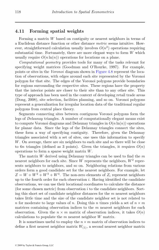
118 Introduction to Spatial Econometrics
4.11 Forming spatial weights
Forming a matrix W based on contiguity or nearest neighbors in terms ofa Euclidean distance function or other distance metric seems intuitive. How-ever, straightforward calculation usually involves O(n2) operations requiringsubstantial time. Fortunately, there are more elegant ways to form W whichusually require O(n ln(n)) operations for locations on a plane.
Computational geometry provides tools for many of the tasks relevant forspecifying weight matrices (Goodman and O’Rourke, 1997). For example,points or sites in the Voronoi diagram shown in Figure 4.8 represent the loca-tion of observations, with edges around each site represented by the Voronoipolygon for that site. The edges of the Voronoi polygons provide boundariesfor regions surrounding the respective sites. These regions have the propertythat the interior points are closer to their site than to any other site. Thistype of approach has been used in the context of developing retail trade areas(Dong, 2008), site selection, facilities planning, and so on. Voronoi polygonsrepresent a generalization for irregular location data of the traditional regularpolygons from central place theory.
Segments connecting sites between contiguous Voronoi polygons form thelegs of Delaunay triangles. A number of computationally elegant means existto compute Voronoi diagrams and Delaunay triangles in O(n ln(n)) operationsfor planar data. Since the legs of the Delaunay triangles connect the sites,these form a way of specifying contiguity. Therefore, given the Delaunaytriangles associated with a set of sites, one uses this information to specifyW . On average, there are six neighbors to each site and so there will be closeto 6n triangles (defined as 3 points). Given the triangles, it requires O(n)operations to form a sparse weight matrix W .
The matrix W derived using Delaunay triangles can be used to find the mnearest neighbors for each site. Since W represents the neighbors, W 2 repre-sents neighbors to neighbors, and so on. Neighboring relations from variousorders form a good candidate set for the nearest neighbors. For example, letZ = W +W 2 +W 3 +W 4. The non-zero elements of Zi represent neighborsup to the fourth order for each observation i. Having identified the candidateobservations, we can use their locational coordinates to calculate the distance(for some chosen metric) from observation i to the candidate neighbors. Sort-ing this short set of candidate neighbor distances for the m nearest neighborstakes little time and the size of the candidate neighbor set is not related ton for moderate to large values of n. Doing this n times yields a set of n×mmatrices containing observation indices to the m nearest neighbors for eachobservation. Given the n × m matrix of observation indices, it takes O(n)calculations to populate the m nearest neighbor W matrix.
It is sometimes useful to employ the n×m matrix of observation indices todefine a first nearest neighbor matrix W(1), a second nearest neighbor matrix
© 2009 by Taylor & Francis Group, LLC
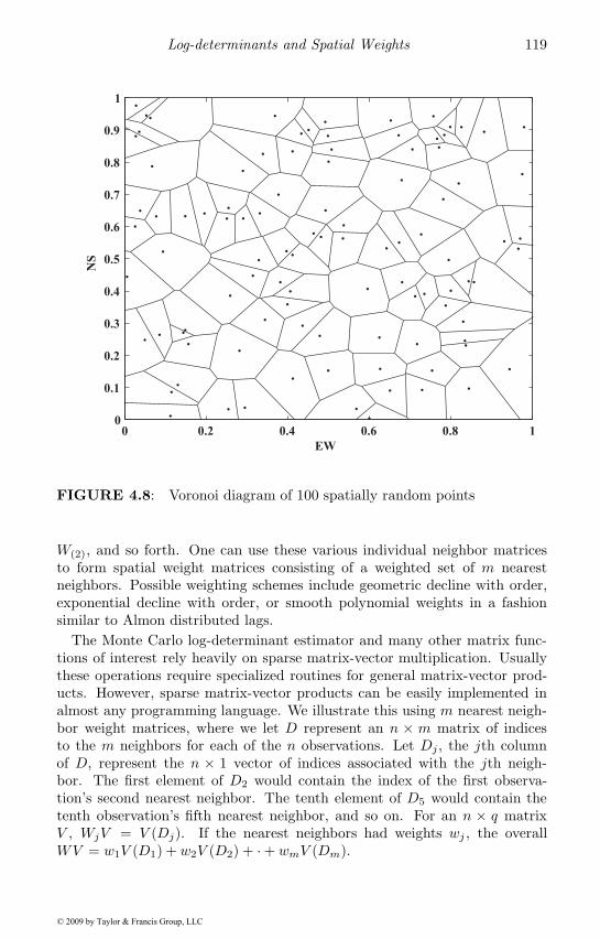
Log-determinants and Spatial Weights 119
0 0.2 0.4 0.6 0.8 10
0.1
0.2
0.3
0.4
0.5
0.6
0.7
0.8
0.9
1
EW
NS
FIGURE 4.8: Voronoi diagram of 100 spatially random points
W(2), and so forth. One can use these various individual neighbor matricesto form spatial weight matrices consisting of a weighted set of m nearestneighbors. Possible weighting schemes include geometric decline with order,exponential decline with order, or smooth polynomial weights in a fashionsimilar to Almon distributed lags.
The Monte Carlo log-determinant estimator and many other matrix func-tions of interest rely heavily on sparse matrix-vector multiplication. Usuallythese operations require specialized routines for general matrix-vector prod-ucts. However, sparse matrix-vector products can be easily implemented inalmost any programming language. We illustrate this using m nearest neigh-bor weight matrices, where we let D represent an n × m matrix of indicesto the m neighbors for each of the n observations. Let Dj , the jth columnof D, represent the n × 1 vector of indices associated with the jth neigh-bor. The first element of D2 would contain the index of the first observa-tion’s second nearest neighbor. The tenth element of D5 would contain thetenth observation’s fifth nearest neighbor, and so on. For an n × q matrixV , WjV = V (Dj). If the nearest neighbors had weights wj , the overallWV = w1V (D1) + w2V (D2) + · + wmV (Dm).
© 2009 by Taylor & Francis Group, LLC
120 Introduction to Spatial Econometrics
A very interesting feature is that for many programming languages thetime required to index a matrix is the same as for a vector, since indexingonly requires altering a row label that pertains to all columns. To illustratethis, we indexed a 1, 000, 000 by 50 matrix and a 1, 000, 000 by 1 vector. InMatlab it took 0.051 seconds to index the matrix and 0.043 seconds to indexthe vector.
We note that sparse matrix-vector products needed to compute the log-determinant estimator and other matrix functions require only indexing andaddition, two of the fastest operations possible on digital computers. Thismeans that nearest neighbor calculations can be implemented in a variety ofcomputing languages such as FORTRAN or C, and various statistical softwareenvironments.
For multivariate and spatiotemporal weight matrices, it may be necessaryto compute the n2 possible distances and sort these to find the m nearestneighbors. Fortunately, partial sorting algorithms exist (see fortran2000.comfor some examples) that require some function of m operations for each sortrather than a function of n. This greatly accelerates formation of multivariateand spatiotemporal weight matrices. Often there exist ways to reduce thenearest neighbor candidate list for each observation. For example, in the caseof a spatiotemporal weight matrix one could require neighbors to be no morethan four years old, which would materially reduce the time required to formspatiotemporal weight matrices spanning a 20 year period.
4.12 Chapter summary
Determinants and other functions of the n × n spatial weight matrix of-ten arise in spatial econometrics. Brute force approaches to dealing withdeterminants and matrix functions limit the possible sample size or the abil-ity to perform more involved estimation or testing. This chapter dealt withthese computational issues. Section 4.1 introduced the need for determinantswhen working with dependent variable transformations of the type that arisein spatial regression models. Section 4.2 described basic approaches to cal-culating determinants. Special features of spatial systems such as sparsitywere discussed in Section 4.3 along with ways to take advantage of sparsityby ordering rows and columns of W when using direct calculations for thelog-determinant.
Section 4.4 introduced a Monte Carlo approximation to the log-determinantthat takes little time and memory and showed that this approach leads to smallerrors in estimation of the dependence parameter, ρ. Similarly, Section 4.5introduced a Chebyshev approximation that also performed well. Section 4.6discussed another approximation approach that treats the sample as arising
© 2009 by Taylor & Francis Group, LLC
Log-determinants and Spatial Weights 121
from an increasing domain process and extrapolates the log-determinant. Sec-tion 4.7 described a few approaches to bounding log-determinants that maybe of both theoretical and practical interest.
Section 4.8 extended the log-determinant approximation techniques to othercommonly encountered tasks that arise in spatial modeling. These includedsolving systems of equations, finding the diagonal of the variance-covariancematrix (without computing the entire variance-covariance matrix), and cal-culating the derivative of the log-determinant. Section 4.9 applied some ofthese techniques to computing the summary measures of impacts (partialderivatives) that are needed for interpretation of spatial econometric models.Section 4.10 showed a method that can be used to produce closed-form solu-tions for a number of spatial models involving a single dependence parameter.Finally, efficient approaches to forming spatial weight matrices were discussedin Section 4.11.
© 2009 by Taylor & Francis Group, LLC
Chapter 5
Bayesian Spatial EconometricModels
This chapter describes application of Bayesian methodology to spatial econo-metric modeling and estimation. Bayesian methodology has existed for a longtime, but recent approaches to estimation of these models have led to a re-vival of interest in these methods. The estimation approach known as MarkovChain Monte Carlo (MCMC) decomposes complicated estimation problemsinto simpler problems that rely on the conditional distributions for each pa-rameter in the model (Gelfand and Smith, 1990). This innovation makesapplication of the Bayesian methodology far easier than past approaches thatrelied on analytical solution of the posterior distribution. A result of this isthat an extensible toolkit for solving spatial econometric estimation problemscan be developed at both a theoretical and applied level.
We begin by introducing Bayesian econometric methodology in Section 5.1.This is followed in Section 5.2 by a conventional Bayesian approach to esti-mating the SAR model, which is shown to require numerical integration overthe spatial dependence parameter ρ. The historical need to carry out nu-merical integration of the posterior distribution with respect to parameters inBayesian models made conventional Bayesian methodology relatively difficultfor models with a large number of parameters.
Section 5.3 introduces Markov Chain Monte Carlo (MCMC) estimation ap-proaches for the family of spatial econometric models discussed in Chapter 2.Bayesian methodology focuses on distributions involving data and parame-ters, which has the effect of structuring estimation problems in such a way asto produce a posterior distribution that can be decomposed into a sequence ofconditional distributions. These “conditionals” characterize the distributionof a single parameter given all other parameters in the model, and they areextremely useful from both a theoretical and applied perspective. From anapplied perspective, conditional distributions are required for Markov ChainMonte Carlo (MCMC) estimation. This method of estimation became pop-ular when Gelfand and Smith (1990) demonstrated that MCMC samplingfrom the sequence of complete conditional distributions for all parameters ina model produces a set of estimates that converge in the limit to the true(joint) posterior distribution of the parameters. Therefore, if we can decom-pose the posterior distribution into a set of conditional distributions for eachparameter in the model, drawing samples from these will provide us with valid
123© 2009 by Taylor & Francis Group, LLC
124 Introduction to Spatial Econometrics
Bayesian parameter estimates. This approach to estimation is the subject ofSections 5.3 and 5.4 with an applied illustration provided in Section 5.5.
One benefit of Bayesian methodology used in conjunction with MCMCestimation is that an extensible toolkit can be devised for dealing with awide array of spatial econometric problems. As a concrete example of this,Section 5.6 extends the conventional spatial regression models from Chapter 2to allow for a heteroscedastic disturbance structure in place of the conventionalassumption of homoscedastic disturbances. Other uses for the MCMC methodare also provided in this section.
Additional material on the MCMC approach to modeling and estimation isprovided in a number of the remaining chapters.
5.1 Bayesian methodology
An important aspect of Bayesian methodology is the focus on distributionsfor the data as well as parameters. Bayes’ rule involves combining the datadistribution embodied in the likelihood function with prior distributions forthe parameters assigned by the practitioner, to produce a posterior distribu-tion for the parameters. The posterior distribution forms the basis for allinference, since it contains all relevant information regarding the estimationproblem. Relevant information includes both sample data information comingfrom the likelihood, as well as prior or subjective information embodied in thedistributions assigned to the parameters.
As noted in Chapter 1, econometric models focus on: 1) estimation andinference about parameters, 2) model specification and model comparisons,and 3) model prediction or out-of-sample forecasting. The Bayesian approachto estimation arises from some basic axioms of probability.1 For two randomvariables A and B we have that the joint probability p(A,B) can be expressedin terms of conditional probability P (A|B) or P (B|A) and the marginal prob-ability P (B) (or P (A)) as shown in (5.1) and (5.2).
p(A,B) = p(A|B)p(B) (5.1)p(A,B) = p(B|A)p(A) (5.2)
Setting these two expressions equal and rearranging gives rise to Bayes’ Rule:
p(B|A) =p(A|B)p(B)
p(A)(5.3)
1See Koop (2003) for a more complete introduction to Bayesian econometrics. Much of thisintroductory material mirrors that presented in the introduction of Koop (2003).
© 2009 by Taylor & Francis Group, LLC
Bayesian Spatial Econometric Models 125
For our purposes, we let D = {y,X,W} represent model data and θ = Bdenote model parameters so that:
p(θ|D) =p(D|θ)p(θ)p(D)
(5.4)
A point to note is that Bayesian modeling assumes the parameters θ have aprior distribution p(θ) that reflects previous knowledge as well as uncertaintywe have prior to observing the data. This distribution is used to provide aformalized probabilistic statement that overtly specifies both prior informa-tion and uncertainty. If we know very little from prior experience, then thisdistribution should represent a vague probabilistic statement, whereas a greatdeal of previous experience would lead to a very narrow distribution centeredon parameter values gained from previous experience.
The left-hand side of (5.4) represents the post-data inference for θ and iscalled the posterior distribution of θ. This represents an update of the priordistribution for the parameter θ after conditioning on the sample data. Theright-hand side of (5.4) indicates that Bayesian parameter inference representsa compromise between prior information embodied in p(θ) and new informa-tion provided by the sample data and model represented by the likelihoodp(D|θ). The Bayesian approach relies on conditional probability to provide aformal structure of rules that allows us to learn (update our prior knowledge)about some unknown quantity such as θ using the model and data.
The nature of the compromise between prior and sample data takes the fol-lowing form. If a spatial sample of data exhibits wide variation across regionsand we are only able to collect a small sample of regions, then the posteriordistribution would place more emphasis on prior experience (the distributionp(θ)) than the distribution implied by the small sample of observable data andmodel contained in the likelihood, p(D|θ). Conversely, if our prior experience(information) was very limited and a great deal of sample data resulted ina likelihood that indicated values of θ distributed tightly around a particu-lar value, then the posterior distribution would place more emphasis on themodel and sample data information, embodied in the likelihood. There is noexplicit process such as this in classical statistics that allows for a tradeoff be-tween prior information and sample data information, since inference is basedentirely on the model and sample data, represented by the likelihood function.
This distinction becomes unimportant for inference based on maximum like-lihood and Bayesian estimation procedures when we have large data samplesand very little prior information. In this situation, both methods rely almostentirely on the sample data information to provide inferences regarding theparameter θ.
Econometric modeling issue 1) is estimation and inference about parame-ters. We note that all Bayesian inference (sometimes called learning) aboutθ|D is based on the posterior density p(θ|D) for the parameters θ given thedata D. We can simplify (5.4) by ignoring the data distribution p(D), sincethis distribution doesn’t involve the parameters θ.
© 2009 by Taylor & Francis Group, LLC
126 Introduction to Spatial Econometrics
p(θ|D) ∝ p(D|θ)p(θ) (5.5)
Expression (5.5) indicates that the posterior distribution of the parame-ter vector θ is a (proportional) product of the term p(D|θ) representing themodel likelihood and the term p(θ) representing the prior distribution for theparameters θ. Since non-Bayesians do not subscribe to the notion that param-eters have prior distributions, they cannot express prior beliefs or uncertaintyabout the parameters using prior distributions.
Econometric modeling issue 2) is model specification and comparison. Givena set i = 1, . . . ,m of Bayesian models, each would be represented by a likeli-hood function and prior distribution as in (5.6).
p(θi|D,Mi) =p(D|θi,Mi)p(θi|Mi)
p(D|Mi)(5.6)
Treating the posterior distributions in this case as conditional on the modelspecification Mi, we can apply Bayes’ rule to expand terms like p(D|Mi) in afashion similar to (5.3). This leads to a set of unconditional posterior modelprobabilities:
p(Mi|D) =p(D|Mi)p(Mi)
p(D)(5.7)
These serve as the basis for inference about different models, given the sampledata. The term p(D|Mi) that appears on the right-hand-side of expression(5.7) is called the marginal likelihood, and we can solve for this key quantityneeded for model comparison finding:
p(D|Mi) =∫p(D|θi,Mi)p(θi|Mi)dθi (5.8)
An important point is the unconditional nature of the model probabilities,which do not depend on the posterior mean parameter values alone, but theentire posterior distribution over which we integrate. Maximum likelihood ap-proaches to model comparison rely on the likelihoods of two models evaluatedat the mean values of the parameter estimates. This means that model com-parison inferences depend on scalar values of the parameter estimates usedto evaluate the likelihood. In contrast, Bayesian model comparison uses theentire posterior distribution of values for the parameters.
Expression (5.8) makes it clear that the theory behind Bayesian modelcomparison is quite simple and follows directly from formal probability ax-ioms of statistics. However, implementation may be hindered by the need tointegrate over the parameter vector θ. We will discuss several approaches todealing with the integration problem in Chapter 6 which is devoted to modelcomparison.
© 2009 by Taylor & Francis Group, LLC
Bayesian Spatial Econometric Models 127
The Bayesian theory for econometric issue 3) requires prediction of an out-of-sample set of observations that we denote y∗ based on sample data ob-servations in D. Here again, we rely on rules of probability to arrive at theposterior distribution of the prediction sample given the sample data D, andmodel parameters θ. This also involves expressing a joint distribution in termsof a conditional and marginal.
p(y∗|D) =∫p(y∗, θ|D)dθ =
∫p(y∗|D, θ)p(θ|D)dθ (5.9)
5.2 Conventional Bayesian treatment of the SAR model
As noted in the previous section, Bayesian methods require analysis of theposterior distribution of the model parameters. This can be carried out usinganalytical or numerical methods. In Section 5.2.1 we show that analyticalapproaches are possible in spatial econometric modeling. However, numer-ical methods for univariate or bivariate integration are required to produceposterior inferences in the family of spatial econometric models discussed inChapter 2, which places limits on both theoretical and applied work. Con-ditioning provides a way to avoid these problems, and is ideally suited tomatch theoretical and MCMC estimation approaches to spatial econometricmodeling.
5.2.1 Analytical approaches to the Bayesian method
As already indicated, one aspect of the Bayesian method is the introductionof prior information in the modeling process. Investigators specify their priorbeliefs using distributions, which are combined with the data distribution toproduce the posterior distribution used for inference. The requirement thatprior beliefs be revealed as part of solving the estimation problem is viewedby some to be a disadvantage of the Bayesian method. We show that in aspatial econometric setting where data samples are typically large, prior in-formation will tend to play a minor role in determining the character of theposterior distribution. The fundamental Bayesian identity works to create amatrix-weighted average of sample and prior information in the posterior, butthe weights are strongly influenced by the quantity of sample data informa-tion available relative to prior information. When large samples are availablethey provide a simplification that can facilitate analytical evaluation of theposterior distribution.
Using the spatial autoregressive model (SAR) from the family of models inChapter 2, we can demonstrate the combination of prior and sample informa-tion. The likelihood for the SAR model: y = ρWy +Xβ + ε, can be written
© 2009 by Taylor & Francis Group, LLC
128 Introduction to Spatial Econometrics
as in (5.10), where we rely on A = (In − ρW ) for notational convenience and|A| denotes the determinant of this matrix.
p(D|β, σ, ρ) = (2πσ2)−n2 |A| exp
(− 1
2σ2(Ay −Xβ)′(Ay −Xβ)
)(5.10)
As noted, we are required to specify prior distributions for the parametersin the model, which will be combined with the likelihood to produce the poste-rior distribution. We might rely on what is known as a normal-inverse gammaprior (NIG) distribution for the parameters β and σ2. This form of priormakes the normal prior distribution for β conditional on an inverse gammadistribution for the parameter σ2. Since the parameter ρ plays such an impor-tant role in this model, and is often a subject of inference, we might specifya uniform prior over the feasible range for this parameter, (1/λmin, 1/λmax),where λmin, λmax represent the minimum and maximum eigenvalues of thespatial weight matrix. As noted in Chapters 2 and 4, row-stochastic spatialweight matrices W typically used in applications of these models lead to ρ inthe interval (λ−1
min, 1).A formal statement of the Bayesian SAR model is shown in (5.11), where
we assume an n×k explanatory variables matrixX . We have added a normal-inverse gamma (NIG) prior for β and σ, with the prior distributions indicatedusing π. This prior specifies that β given σ is distributed multivariate normalN(c, σ2T ), and the marginal distribution for σ takes the form of an inversegamma density denoted IG(a, b) in (5.12).
y = ρWy +Xβ + ε (5.11)ε ∼ N(0, σ2In)
π(β, σ2) ∼ NIG(c, T, a, b)= π(β|σ2)π(σ2)= N(c, σ2T )IG(a, b) (5.12)
=ba
(2π)k/2|T |1/2Γ(a)(σ2)−(a+(k/2)+1)
× exp[−{(β − c)′T−1(β − c) + 2b}/(2σ2)]
π(σ2) =ba
Γ(a)(σ2)−(a+1)exp(−b/σ2) (5.13)
σ2 > 0, a, b > 0π(ρ) ∼ U(λ−1
min, λ−1max)
Note that we have parameterized the inverse-gamma distribution in (5.13),where Γ(·) represents the standard gamma function, Γ(a) =
∫∞0ta−1e−tdt.
The parameters used to specify our prior beliefs are those from the NIG
© 2009 by Taylor & Francis Group, LLC
Bayesian Spatial Econometric Models 129
prior, c, T, a, b, and might also include prior parameters for ρ if we relied ona different type of informative prior for this model parameter.
In cases where we have a great deal of prior uncertainty regarding theparameters β, we can set c = 0, and assign a very large prior variance forβ with zero covariance between parameters in the vector β. This might beaccomplished by setting T = Ik · 1010, or some other large magnitude. This isknown as a diffuse or uninformative prior. An uninformative prior can be setfor the parameter σ2 by assigning values of a = b = 0. We will argue shortlythat this approach is intuitively reasonable when dealing with large spatialdata sets. For ρ, we assign a prior that indicates all outcomes within thefeasible range (λ−1
min, λ−1max) are equally probable. An additional point to note
is that we assume independence between the prior assigned to β and σ2 andthat for ρ. Prior independence does not imply independence in the posteriordistributions of the model parameters, it simply reflects prior beliefs whichcan be inconsistent with posterior outcomes.
From Bayes’ Theorem we know that the posterior distribution for the modelparameters takes the form:
p(β, σ2, ρ|D) =p(D|β, σ2, ρ)π(β, σ2)π(ρ)
p(D)(5.14)
By multiplying the expression for the likelihood and prior we can determinethe form of the posterior up to a constant term, p(D), that does not involvethe model parameters. An identity in (5.15) that has been labeled completingthe square is useful in arriving at the result shown in (5.16).
(Ay −Xβ)′(Ay −Xβ) + (β − c)′T−1(β − c) + 2b≡ (β − c∗)′(T ∗)−1(β − c∗) + 2b∗ (5.15)
p(β, σ2, ρ|D) ∝ (σ2)a∗+(k/2)+1 |A|
× exp{− 12σ2
[2b∗ + (β − c∗)′(T ∗)−1(β − c∗)]} (5.16)
c∗ = (X ′X + T−1)−1(X ′Ay + T−1c)T ∗ = (X ′X + T−1)−1
a∗ = a+ n/2b∗ = b+
(c′T−1c+ y′A′Ay − (c∗)′(T ∗)−1c∗
)/2
A = In − ρW
One thing to note concerning this result is that the usual case for non-spatial regression models where the NIG prior serves as a conjugate priordistribution does not hold here (Zellner, 1971). A general definition of con-jugate prior distributions are those that result in computationally tractable
© 2009 by Taylor & Francis Group, LLC
130 Introduction to Spatial Econometrics
posterior distributions, and this term is often used to refer to situations wherethe posterior distribution takes the same form as the prior distribution exceptthat model parameters are updated. In the case of a non-spatial regressionmodel an NIG(c, T, a, b) prior placed on the parameters β and σ would resultin an NIG(c∗, T ∗, a∗, b∗) posterior distribution for these parameters, wherewe use the star superscript to denote parameter updating. This would be theresult if ρ = 0, so that A = In in expression (5.16).
Because of the informative prior distributions used in this model, mattersbecome complicated in two ways. First, there is the need to specify or assignvalues for the parameters of the NIG prior distribution. Second, the posteriordistribution in (5.16) is difficult to analyze because it requires integration ofσ2 as well as ρ to arrive at a posterior expression for β. Similarly, it requiresthat we integrate with respect to β and ρ to find the posterior for σ2. Weshould ask the question — is the prior information likely to exert an impacton our inferences regarding β? If not, we can greatly simplify the posterior in(5.16), by relying on uninformative priors.
We note that the term: y′A′Ay − (c∗)′(T ∗)−1c∗ would equal the sum ofsquared residuals from the SAR model if we knew the posterior means for theparameters ρ and c∗. This implies that the ratio b∗/a∗ would be approximatelyequal to the residual sum of squares for the case where a, b → 0 and T−1 →0. These NIG prior parameter settings would result in uninformative priordistributions assigned to the parameters β and σ2.
5.2.2 Analytical solution of the Bayesian spatial model
It is worthwhile to pursue solution of the Bayesian SAR model in the con-text of simplifications offered by a non-informative prior (Hepple, 1995a,b).We replace the NIG prior from the previous section with an uninformativeprior based on a, b = 0 and T−1 = 0, and assume independence betweenthe prior assigned to ρ and that for β and σ, i.e., π(β, σ, ρ) = π(β, σ)π(ρ).Using this type of prior and applying Bayes’ Theorem that combines thelikelihood and prior leads to the simplified posterior distribution shown in(5.17). This result is consistent with our earlier observation relating the term:y′A′Ay − (c∗)′(T ∗)−1c∗ and the residual sum of squares.
p(β, σ, ρ|D) ∝ p(D|β, σ, ρ) · π(β, σ) · π(ρ) (5.17)
∝ σ−n−1 |A| exp(− 1
2σ2(Ay −Xβ)′(Ay −Xβ)
)π(ρ)
With this simpler posterior, we can treat σ as a nuisance parameter andanalytically integrate this out of the expression in (5.17). This can be accom-plished using properties of the inverse gamma distribution, leading to:
© 2009 by Taylor & Francis Group, LLC
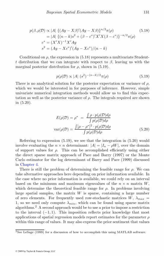
Bayesian Spatial Econometric Models 131
p(β, ρ|D) ∝ |A| {(Ay −Xβ)′(Ay −Xβ)}n/2π(ρ) (5.18)= |A| {(n− k)s2 + (β − c∗)′X ′X(β − c∗)}−n/2π(ρ)
c∗ = (X ′X)−1X ′Ays2 = (Ay −Xc∗)′(Ay −Xc∗)/(n− k)
Conditional on ρ, the expression in (5.18) represents a multivariate Student-t distribution that we can integrate with respect to β, leaving us with themarginal posterior distribution for ρ, shown in (5.19).
p(ρ|D) ∝ |A| (s2)−(n−k)/2π(ρ) (5.19)
There is no analytical solution for the posterior expectation or variance of ρ,which we would be interested in for purposes of inference. However, simpleunivariate numerical integration methods would allow us to find this expec-tation as well as the posterior variance of ρ. The integrals required are shownin (5.20).
E(ρ|D) = ρ∗ =∫ρ · p(ρ|D)dρ∫p(ρ|D)dρ
var(ρ|D) =∫[ρ− ρ∗]2 · p(ρ|D)dρ∫
p(ρ|D)dρ(5.20)
Referring to expression (5.19), we see that the integration in (5.20) wouldinvolve evaluating the n× n determinant: |A| = |In − ρW |, over the domainof support values for ρ. This can be accomplished efficiently using eitherthe direct sparse matrix approach of Pace and Barry (1997) or the MonteCarlo estimator for the log determinant of Barry and Pace (1999) discussedin Chapter 4.
There is still the problem of determining the feasible range for ρ. We cantake alternative approaches here depending on prior information available. Inthe case where no prior information is available, we could rely on an intervalbased on the minimum and maximum eigenvalues of the n × n matrix W ,which determine the theoretical feasible range for ρ. In problems involvinglarge spatial samples, the matrix W is sparse, containing a large numberof zero elements. For frequently used row-stochastic matrices W , λmax =1, so we need only compute λmin, which can be found using sparse matrixalgorithms.2 A second approach would be to use a prior to impose a restrictionto the interval (−1, 1). This imposition reflects prior knowledge that mostapplications of spatial regression models report estimates for the parameter ρwithin this range of values. It may also express the prior sentiment that values
2See LeSage (1999) for a discussion of how to accomplish this using MATLAB software.
© 2009 by Taylor & Francis Group, LLC
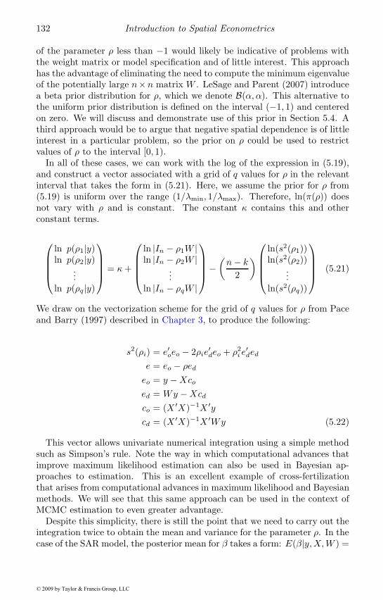
132 Introduction to Spatial Econometrics
of the parameter ρ less than −1 would likely be indicative of problems withthe weight matrix or model specification and of little interest. This approachhas the advantage of eliminating the need to compute the minimum eigenvalueof the potentially large n×n matrix W . LeSage and Parent (2007) introducea beta prior distribution for ρ, which we denote B(α, α). This alternative tothe uniform prior distribution is defined on the interval (−1, 1) and centeredon zero. We will discuss and demonstrate use of this prior in Section 5.4. Athird approach would be to argue that negative spatial dependence is of littleinterest in a particular problem, so the prior on ρ could be used to restrictvalues of ρ to the interval [0, 1).
In all of these cases, we can work with the log of the expression in (5.19),and construct a vector associated with a grid of q values for ρ in the relevantinterval that takes the form in (5.21). Here, we assume the prior for ρ from(5.19) is uniform over the range (1/λmin, 1/λmax). Therefore, ln(π(ρ)) doesnot vary with ρ and is constant. The constant κ contains this and otherconstant terms.
⎛⎜⎜⎜⎝ln p(ρ1|y)ln p(ρ2|y)
...ln p(ρq|y)
⎞⎟⎟⎟⎠ = κ+
⎛⎜⎜⎜⎝ln |In − ρ1W |ln |In − ρ2W |
...ln |In − ρqW |
⎞⎟⎟⎟⎠−(n− k
2
)⎛⎜⎜⎜⎝ln(s2(ρ1))ln(s2(ρ2))
...ln(s2(ρq))
⎞⎟⎟⎟⎠ (5.21)
We draw on the vectorization scheme for the grid of q values for ρ from Paceand Barry (1997) described in Chapter 3, to produce the following:
s2(ρi) = e′oeo − 2ρie′deo + ρ2i e
′ded
e = eo − ρed
eo = y −Xco
ed = Wy −Xcd
co = (X ′X)−1X ′ycd = (X ′X)−1X ′Wy (5.22)
This vector allows univariate numerical integration using a simple methodsuch as Simpson’s rule. Note the way in which computational advances thatimprove maximum likelihood estimation can also be used in Bayesian ap-proaches to estimation. This is an excellent example of cross-fertilizationthat arises from computational advances in maximum likelihood and Bayesianmethods. We will see that this same approach can be used in the context ofMCMC estimation to even greater advantage.
Despite this simplicity, there is still the point that we need to carry out theintegration twice to obtain the mean and variance for the parameter ρ. In thecase of the SAR model, the posterior mean for β takes a form: E(β|y,X,W ) =
© 2009 by Taylor & Francis Group, LLC
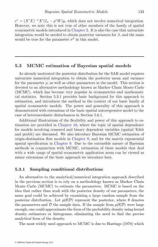
Bayesian Spatial Econometric Models 133
c∗ = (X ′X)−1X ′(In − ρ∗W )y, which does not involve numerical integration.However, we note this is not true of other members of the family of spatialeconometric models introduced in Chapter 2. It is also the case that univariateintegration would be needed to obtain posterior variances for β, and the samewould be true for the parameter σ2 in this model.
5.3 MCMC estimation of Bayesian spatial models
As already motivated the posterior distribution for the SAR model requiresunivariate numerical integration to obtain the posterior mean and variancefor the parameter ρ, as well as other parameters in the model. This section isdevoted to an alternative methodology known as Markov Chain Monte Carlo(MCMC), which has become very popular in econometrics and mathemati-cal statistics. Section 5.3.1 provides basic background for this approach toestimation, and introduces the method in the context of our basic family ofspatial econometric models. The power and generality of this approach isdemonstrated with extensions of the basic spatial autoregressive model to thecase of heteroscedastic disturbances in Section 5.6.1.
Additional illustrations of the flexibility and power of this approach to es-timation are provided in Chapter 10, where the topic of spatial dependencefor models involving censored and binary dependent variables (spatial Tobitand probit) are discussed. We also introduce Bayesian MCMC estimation oforigin-destination flow models in Chapter 8, and for the matrix exponentialspatial specification in Chapter 9. Due to the extensible nature of Bayesianmethods in conjunction with MCMC, estimation of these models that dealwith a wide range of spatial econometric application areas can be viewed asminor extensions of the basic approach we introduce here.
5.3.1 Sampling conditional distributions
An alternative to the analytical/numerical integration approach describedin the previous section is to rely on a methodology known as Markov ChainMonte Carlo (MCMC) to estimate the parameters. MCMC is based on theidea that rather than work with the posterior density of our parameters, thesame goal could be achieved by examining a large random sample from theposterior distribution. Let p(θ|D) represent the posterior, where θ denotesthe parameters and D the sample data. If the sample from p(θ|D) were largeenough, one could approximate the form of the probability density using kerneldensity estimators or histograms, eliminating the need to find the preciseanalytical form of the density.
The most widely used approach to MCMC is due to Hastings (1970) which
© 2009 by Taylor & Francis Group, LLC
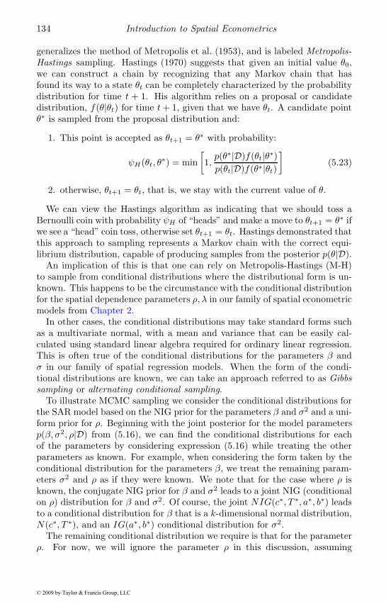
134 Introduction to Spatial Econometrics
generalizes the method of Metropolis et al. (1953), and is labeled Metropolis-Hastings sampling. Hastings (1970) suggests that given an initial value θ0,we can construct a chain by recognizing that any Markov chain that hasfound its way to a state θt can be completely characterized by the probabilitydistribution for time t + 1. His algorithm relies on a proposal or candidatedistribution, f(θ|θt) for time t+ 1, given that we have θt. A candidate pointθ∗ is sampled from the proposal distribution and:
1. This point is accepted as θt+1 = θ∗ with probability:
ψH(θt, θ∗) = min[1,p(θ∗|D)f(θt|θ∗)p(θt|D)f(θ∗|θt)
](5.23)
2. otherwise, θt+1 = θt, that is, we stay with the current value of θ.
We can view the Hastings algorithm as indicating that we should toss aBernoulli coin with probability ψH of “heads” and make a move to θt+1 = θ∗ ifwe see a “head” coin toss, otherwise set θt+1 = θt. Hastings demonstrated thatthis approach to sampling represents a Markov chain with the correct equi-librium distribution, capable of producing samples from the posterior p(θ|D).
An implication of this is that one can rely on Metropolis-Hastings (M-H)to sample from conditional distributions where the distributional form is un-known. This happens to be the circumstance with the conditional distributionfor the spatial dependence parameters ρ, λ in our family of spatial econometricmodels from Chapter 2.
In other cases, the conditional distributions may take standard forms suchas a multivariate normal, with a mean and variance that can be easily cal-culated using standard linear algebra required for ordinary linear regression.This is often true of the conditional distributions for the parameters β andσ in our family of spatial regression models. When the form of the condi-tional distributions are known, we can take an approach referred to as Gibbssampling or alternating conditional sampling.
To illustrate MCMC sampling we consider the conditional distributions forthe SAR model based on the NIG prior for the parameters β and σ2 and a uni-form prior for ρ. Beginning with the joint posterior for the model parametersp(β, σ2, ρ|D) from (5.16), we can find the conditional distributions for eachof the parameters by considering expression (5.16) while treating the otherparameters as known. For example, when considering the form taken by theconditional distribution for the parameters β, we treat the remaining param-eters σ2 and ρ as if they were known. We note that for the case where ρ isknown, the conjugate NIG prior for β and σ2 leads to a joint NIG (conditionalon ρ) distribution for β and σ2. Of course, the joint NIG(c∗, T ∗, a∗, b∗) leadsto a conditional distribution for β that is a k-dimensional normal distribution,N(c∗, T ∗), and an IG(a∗, b∗) conditional distribution for σ2.
The remaining conditional distribution we require is that for the parameterρ. For now, we will ignore the parameter ρ in this discussion, assuming
© 2009 by Taylor & Francis Group, LLC
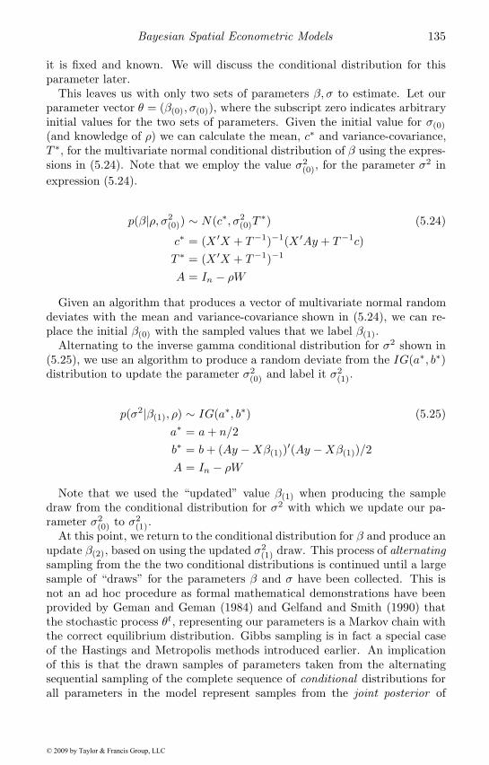
Bayesian Spatial Econometric Models 135
it is fixed and known. We will discuss the conditional distribution for thisparameter later.
This leaves us with only two sets of parameters β, σ to estimate. Let ourparameter vector θ = (β(0), σ(0)), where the subscript zero indicates arbitraryinitial values for the two sets of parameters. Given the initial value for σ(0)
(and knowledge of ρ) we can calculate the mean, c∗ and variance-covariance,T ∗, for the multivariate normal conditional distribution of β using the expres-sions in (5.24). Note that we employ the value σ2
(0), for the parameter σ2 inexpression (5.24).
p(β|ρ, σ2(0)) ∼ N(c∗, σ2
(0)T∗) (5.24)
c∗ = (X ′X + T−1)−1(X ′Ay + T−1c)T ∗ = (X ′X + T−1)−1
A = In − ρW
Given an algorithm that produces a vector of multivariate normal randomdeviates with the mean and variance-covariance shown in (5.24), we can re-place the initial β(0) with the sampled values that we label β(1).
Alternating to the inverse gamma conditional distribution for σ2 shown in(5.25), we use an algorithm to produce a random deviate from the IG(a∗, b∗)distribution to update the parameter σ2
(0) and label it σ2(1).
p(σ2|β(1), ρ) ∼ IG(a∗, b∗) (5.25)a∗ = a+ n/2b∗ = b+ (Ay −Xβ(1))′(Ay −Xβ(1))/2A = In − ρW
Note that we used the “updated” value β(1) when producing the sampledraw from the conditional distribution for σ2 with which we update our pa-rameter σ2
(0) to σ2(1).
At this point, we return to the conditional distribution for β and produce anupdate β(2), based on using the updated σ2
(1) draw. This process of alternatingsampling from the the two conditional distributions is continued until a largesample of “draws” for the parameters β and σ have been collected. This isnot an ad hoc procedure as formal mathematical demonstrations have beenprovided by Geman and Geman (1984) and Gelfand and Smith (1990) thatthe stochastic process θt, representing our parameters is a Markov chain withthe correct equilibrium distribution. Gibbs sampling is in fact a special caseof the Hastings and Metropolis methods introduced earlier. An implicationof this is that the drawn samples of parameters taken from the alternatingsequential sampling of the complete sequence of conditional distributions forall parameters in the model represent samples from the joint posterior of
© 2009 by Taylor & Francis Group, LLC
136 Introduction to Spatial Econometrics
the model parameters. Recall, this is the basis for all inference in Bayesiananalysis.
Having a large sample of parameters from the posterior distribution allowsus to proceed with inference regarding the model parameters β and σ, whichwould be based on statistics such as the mean and standard deviation com-puted from these sampled parameter draws. In fact, given a large enoughsample of parameters, we could use kernel density estimation procedures toconstruct the entire posterior distribution of the parameters, not simply themean and standard deviation point estimates.
5.3.2 Sampling for the parameter ρ
To this point, we have assumed unrealistically that the parameter ρ from ourmodel is known. To complete our scheme for MCMC estimation of the SARmodel we need to sample the parameter ρ from its conditional distribution.This takes the form:
p(ρ|β, σ) ∝ p(ρ, β, σ|D)p(β, σ|D)
∝ |In − ρW |exp(− 1
2σ2(Ay −Xβ)′(Ay −Xβ)
)(5.26)
This conditional distribution does not take a known form as in the caseof the conditionals for the parameters β and σ where we had normal andinverse gamma distributions. Sampling for the parameter ρ must proceed us-ing an alternative approach, such as Metropolis-Hastings. We will combineMetropolis-Hastings (M-H) sampling for the parameter ρ in our model andGibbs sampling from the normal and inverse gamma distributions for the pa-rameters β and σ to produce MCMC estimates for the SAR model (LeSage,1997). This type of procedure is often labeled Metropolis within Gibbs sam-pling.
For (M-H) sampling we require a proposal distribution from which we gener-ate a candidate value for the parameter ρ, which we label ρ∗. This candidatevalue as well as the current value that we label ρc are evaluated in expression(5.26) to calculate an acceptance probability using (5.27).
ψH(ρc, ρ∗) = min[1,p(ρ∗|β, σ)p(ρc|β, σ)
](5.27)
We use a normal distribution as the proposal distribution along with atuned random-walk procedure suggested by Holloway, Shankara, and Rahman(2002) to produce the candidate values for ρ. The procedure involves useof the current value ρc, a random deviate drawn from a standard normaldistribution, and a tuning parameter c as shown in (5.28).
© 2009 by Taylor & Francis Group, LLC
Bayesian Spatial Econometric Models 137
ρ∗ = ρc + c ·N(0, 1) (5.28)
Expression (5.28) should make it clear why this type of proposal generatingprocedure is labeled a random-walk procedure. The goal of tuning the propos-als coming from the normal proposal distribution is to ensure that the M-Hsampling procedure moves over the entire conditional distribution. We wouldlike the proposal to produce draws from the dense part of this distributionand avoid a situation where the sampler is stuck in a very low density part ofthe conditional distribution where the density or support is low.
To achieve this goal, the tuning parameter c in (5.28) is adjusted based onmonitoring the acceptance rates from the M-H procedure during the MCMCdrawing procedure. Specifically, if the acceptance rate falls below 40%, weadjust c′ = c/1.1, which decreases the variance of the normal random deviatesproduced by the proposal distribution, so that new proposals are more closelyrelated to the current value ρc. This should lead to an increased acceptancerate. If the acceptance rate rises above 60%, we adjust c′ = (1.1)c, whichincreases the variance of the normal random deviates so that new proposalsrange more widely over the domain of the parameter ρ. This should result ina lower acceptance rate. The goal is to achieve a situation where the tuningparameter settles to a fixed value resulting in an acceptance rate between 40and 60 percent. At this point, no further adjustments to the tuning parametertake place and we continue to sample from the normal proposal distributionusing the resulting tuned value of c.
There is a need to resort to tuning the proposal distribution because smallsample sizes result in the parameter ρ having a conditional distribution thatexhibits a wide dispersion, whereas large sample sizes usually produce a smalldispersion since this parameter is estimated quite precisely in these circum-stances. This means that a single setting for the tuning parameter will notwork well in all circumstances, whereas this adaptive feedback tuning pro-cedure will accommodate different samples arising from varying estimationproblems. Figure 5.1 shows a plot of the acceptance rates along with the M-H draws for the parameter ρ associated with the first 250 draws to illustratethese issues. From the top half of the figure showing the monitored acceptancerates, we see that numerous adjustments to the tuning parameter take placeduring the first 50 passes through the MCMC sampling procedure. Theseadjustments stop after the first 100 draws and the M-H sampling procedureproduces a relatively steady acceptance rate just under 50 percent.
The movement of the M-H sampler for the parameter ρ can be seen inthe bottom half of the figure. We see sequences of draws for which the M-Hprocedure continues to reject candidate values in favor of keeping the currentvalue. Both the acceptance rate as well as the sequence of draws can beexamined as a way of detecting problems with the MCMC sampler. Forexample, a long sequence of rejections (a flat line in the plot of draws) wouldbe indicative of the sampler getting stuck. In a wide range of applied situations
© 2009 by Taylor & Francis Group, LLC
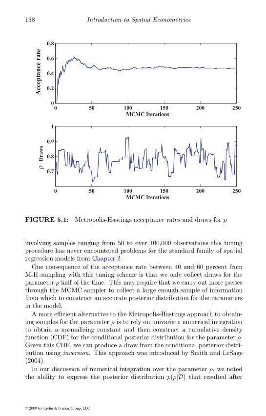
138 Introduction to Spatial Econometrics
0 50 100 150 200 2500
0.2
0.4
0.6
0.8
Acc
epta
nce
rate
MCMC Iterations
0 50 100 150 200 250
0.7
0.8
0.9
1
MCMC Iterations
ρ D
raw
s
FIGURE 5.1: Metropolis-Hastings acceptance rates and draws for ρ
involving samples ranging from 50 to over 100,000 observations this tuningprocedure has never encountered problems for the standard family of spatialregression models from Chapter 2.
One consequence of the acceptance rate between 40 and 60 percent fromM-H sampling with this tuning scheme is that we only collect draws for theparameter ρ half of the time. This may require that we carry out more passesthrough the MCMC sampler to collect a large enough sample of informationfrom which to construct an accurate posterior distribution for the parametersin the model.
A more efficient alternative to the Metropolis-Hastings approach to obtain-ing samples for the parameter ρ is to rely on univariate numerical integrationto obtain a normalizing constant and then construct a cumulative densityfunction (CDF) for the conditional posterior distribution for the parameter ρ.Given this CDF, we can produce a draw from the conditional posterior distri-bution using inversion. This approach was introduced by Smith and LeSage(2004).
In our discussion of numerical integration over the parameter ρ, we notedthe ability to express the posterior distribution p(ρ|D) that resulted after
© 2009 by Taylor & Francis Group, LLC
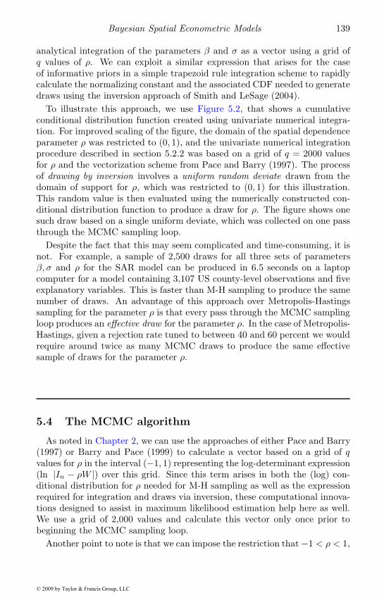
Bayesian Spatial Econometric Models 139
analytical integration of the parameters β and σ as a vector using a grid ofq values of ρ. We can exploit a similar expression that arises for the caseof informative priors in a simple trapezoid rule integration scheme to rapidlycalculate the normalizing constant and the associated CDF needed to generatedraws using the inversion approach of Smith and LeSage (2004).
To illustrate this approach, we use Figure 5.2, that shows a cumulativeconditional distribution function created using univariate numerical integra-tion. For improved scaling of the figure, the domain of the spatial dependenceparameter ρ was restricted to (0, 1), and the univariate numerical integrationprocedure described in section 5.2.2 was based on a grid of q = 2000 valuesfor ρ and the vectorization scheme from Pace and Barry (1997). The processof drawing by inversion involves a uniform random deviate drawn from thedomain of support for ρ, which was restricted to (0, 1) for this illustration.This random value is then evaluated using the numerically constructed con-ditional distribution function to produce a draw for ρ. The figure shows onesuch draw based on a single uniform deviate, which was collected on one passthrough the MCMC sampling loop.
Despite the fact that this may seem complicated and time-consuming, it isnot. For example, a sample of 2,500 draws for all three sets of parametersβ, σ and ρ for the SAR model can be produced in 6.5 seconds on a laptopcomputer for a model containing 3,107 US county-level observations and fiveexplanatory variables. This is faster than M-H sampling to produce the samenumber of draws. An advantage of this approach over Metropolis-Hastingssampling for the parameter ρ is that every pass through the MCMC samplingloop produces an effective draw for the parameter ρ. In the case of Metropolis-Hastings, given a rejection rate tuned to between 40 and 60 percent we wouldrequire around twice as many MCMC draws to produce the same effectivesample of draws for the parameter ρ.
5.4 The MCMC algorithm
As noted in Chapter 2, we can use the approaches of either Pace and Barry(1997) or Barry and Pace (1999) to calculate a vector based on a grid of qvalues for ρ in the interval (−1, 1) representing the log-determinant expression(ln |In − ρW |) over this grid. Since this term arises in both the (log) con-ditional distribution for ρ needed for M-H sampling as well as the expressionrequired for integration and draws via inversion, these computational innova-tions designed to assist in maximum likelihood estimation help here as well.We use a grid of 2,000 values and calculate this vector only once prior tobeginning the MCMC sampling loop.
Another point to note is that we can impose the restriction that −1 < ρ < 1,
© 2009 by Taylor & Francis Group, LLC
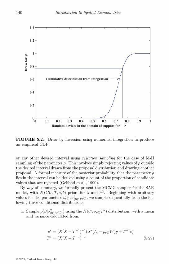
140 Introduction to Spatial Econometrics
0 0.1 0.2 0.3 0.4 0.5 0.6 0.7 0.8 0.9 10
0.2
0.4
0.6
0.8
1
1.2
1.4
ρ
Dra
w f
or ρ
Cumulative distribution from integration ------ >
Random deviate in the domain of support for
FIGURE 5.2: Draw by inversion using numerical integration to producean empirical CDF
or any other desired interval using rejection sampling for the case of M-Hsampling of the parameter ρ. This involves simply rejecting values of ρ outsidethe desired interval drawn from the proposal distribution and drawing anotherproposal. A formal measure of the posterior probability that the parameter ρlies in the interval can be derived using a count of the proportion of candidatevalues that are rejected (Gelfand et al., 1990).
By way of summary, we formally present the MCMC sampler for the SARmodel, with NIG(c, T, a, b) priors for β and σ2. Beginning with arbitraryvalues for the parameters β(0), σ
2(0), ρ(0), we sample sequentially from the fol-
lowing three conditional distributions.
1. Sample p(β|σ2(0), ρ(0)) using the N(c∗, σ(0)T
∗) distribution. with a meanand variance calculated from:
c∗ = (X ′X + T−1)−1(X ′(In − ρ(0)W )y + T−1c)
T ∗ = (X ′X + T−1)−1 (5.29)
© 2009 by Taylor & Francis Group, LLC
Bayesian Spatial Econometric Models 141
Label the sampled parameter vector β(1) and use this to replace theparameter vector β(0).
2. Sample p(σ2|β(1), ρ(0)), using an inverse gamma distribution IG(a∗, b∗).
p(σ2|β(1), ρ) ∼ IG(a∗, b∗) (5.30)a∗ = a+ n/2b∗ = b + (Ay −Xβ(1))′((Ay −Xβ(1))/2A = In − ρ(0)W
3. Sample p(ρ|β(1), σ2(1)), using either the M-H algorithm or integration
and draw by inversion approach set forth in Section 5.3.2. Label thisupdated value ρ(1) and return to step 1.
One sequence of steps 1 to 3 constitute a single pass through the sampler.We carry out a large number of passes and after some initial burn-in period wecollect the draws for the parameters from each pass. For example, we mightcarry out 7,500 draws excluding the first 2,500 and use the resulting sampleto produce posterior estimates and inferences.
The first 2,500 are excluded to account for start-up, or burn-in of the sam-pler. We need to be confident that the MCMC sampling procedure has reachedthe steady state or equilibrium distribution motivated by Hastings (1970). Inpractice, one can produce samples from a short run of 2,500 draws with thefirst 500 excluded for burn-in and compare the means and standard deviationsof the parameters from this run to those obtained from a longer run based ondifferent starting values for the parameters. If the estimates and inferences areequivalent, then there are no likely problems with convergence of the MCMCsampler to a steady state. Once the sampler achieves a steady-state, we in-terpret the draws as coming from the posterior distribution. LeSage (1999)discusses a number of alternative statistical tests that can be applied to thesampled draws as a diagnostic check for convergence.
In the Bayesian MCMC literature, a great deal of attention is devoted toissues regarding convergence of samplers. However, the simple spatial regres-sion models considered here do not encounter problems in this regard. Thisis not to say that attention should not be paid to issues of scaling trans-formations applied to variables and possible collinearity problems betweenexplanatory variables in the model. However, these problems would likelyexert an adverse impact on maximum likelihood estimates as well, especiallyon inferences based on variances calculated using a numerical estimate of theHessian.
© 2009 by Taylor & Francis Group, LLC
142 Introduction to Spatial Econometrics
5.5 An applied illustration
We provide an illustration of Bayesian estimation and inference using a datasample from Pace and Barry (1997) containing voter turnout rates in 3,107 UScounties during the 1980 presidential election. We use the (logged) proportionof voting age population that voted in the election as the dependent variabley, and measures of education, home ownership and income as explanatoryvariables, along with a constant term. The education and home ownershipvariables were expressed as (logged) population of voting age with high schooldegrees and (logged) population owning homes, and the median householdincome variable was also logged. Since all variables are logged, the coefficientestimates have an elasticity interpretation.
We wish to demonstrate that the Bayesian MCMC sampling procedureswill produce nearly identical estimates and inferences as maximum likelihoodmethods when uninformative priors are assigned to the parameters β and σ.In this application we rely on a Beta prior distribution for ρ that we labelB(d, d) introduced by LeSage and Parent (2007). This distribution is shownin (5.31) where Beta(d, d), d > 0 represents the Beta function, Beta(d, d) =∫ 1
0 td−1(1 − t)d−1dt. This prior distribution takes the form of a relatively
uniform distribution centered on a mean value of zero for the parameter ρ.This represents an alternative to the uniform prior on the interval (−1, 1).
π(ρ) ∼ 1Beta(d, d)
(1 + ρ)d−1(1 − ρ)d−1
22d−1(5.31)
Figure 5.3 depicts prior distributions associated with prior values d =1.01, 1.1 and 2, for the B(d, d) prior. From the figure, we see that valuesof d near unity produce a relatively uninformative prior that places zero priorweight on end points of the interval for ρ, consistent with theoretical restric-tions. In the figure, we use the interval (−1, 1) for the parameter ρ whichshould incorporate the effective domain of support for the posterior distribu-tion in most applied work, so this works well as a prior.
The prior mean of the multivariate normal distribution assigned to the pa-rameters β was zero and a diagonal prior variance-covariance structure basedon a scalar variance of 1e+ 12 was used. This creates an uninformative priordistribution that is centered on zero, but whose variance is extremely largeresulting in a nearly uniform prior. Finally, the prior distribution assigned forthe parameter σ2 was based on an inverse gamma distribution, IG(a, b), withthe parameters a = b = 0, which results in a diffuse or non-informative priorfor this parameter.
In addition to demonstrating equivalent estimates and inferences from max-imum likelihood and Bayesian procedures when using relatively uninformativepriors, we would also like to illustrate that equivalent posterior distributions
© 2009 by Taylor & Francis Group, LLC
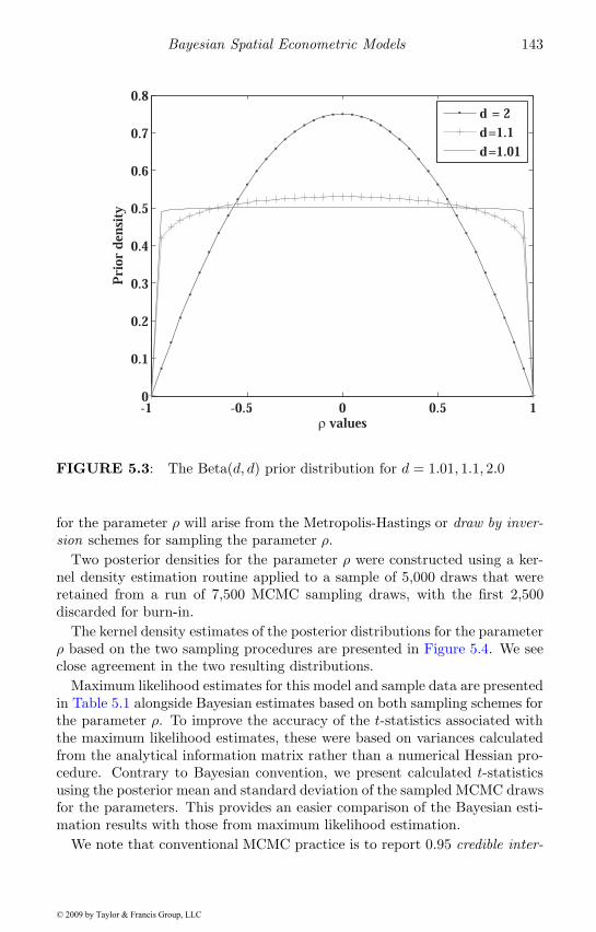
Bayesian Spatial Econometric Models 143
-1 -0.5 0 0.5 10
0.1
0.2
0.3
0.4
0.5
0.6
0.7
0.8
ρ values
Pri
or d
ensi
ty
d = 2d=1.1d=1.01
FIGURE 5.3: The Beta(d, d) prior distribution for d = 1.01, 1.1, 2.0
for the parameter ρ will arise from the Metropolis-Hastings or draw by inver-sion schemes for sampling the parameter ρ.
Two posterior densities for the parameter ρ were constructed using a ker-nel density estimation routine applied to a sample of 5,000 draws that wereretained from a run of 7,500 MCMC sampling draws, with the first 2,500discarded for burn-in.
The kernel density estimates of the posterior distributions for the parameterρ based on the two sampling procedures are presented in Figure 5.4. We seeclose agreement in the two resulting distributions.
Maximum likelihood estimates for this model and sample data are presentedin Table 5.1 alongside Bayesian estimates based on both sampling schemes forthe parameter ρ. To improve the accuracy of the t-statistics associated withthe maximum likelihood estimates, these were based on variances calculatedfrom the analytical information matrix rather than a numerical Hessian pro-cedure. Contrary to Bayesian convention, we present calculated t-statisticsusing the posterior mean and standard deviation of the sampled MCMC drawsfor the parameters. This provides an easier comparison of the Bayesian esti-mation results with those from maximum likelihood estimation.
We note that conventional MCMC practice is to report 0.95 credible inter-
© 2009 by Taylor & Francis Group, LLC
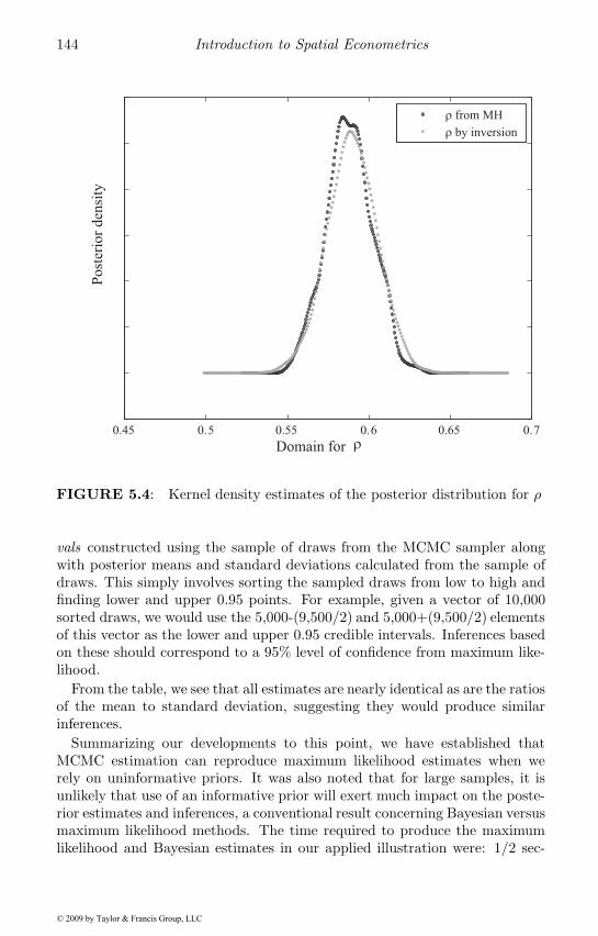
144 Introduction to Spatial Econometrics
0.45 0.5 0.55 0.6 0.65 0.7
Domain for ρ
ρ from MH
ρ by inversion
Post
erio
r den
sity
FIGURE 5.4: Kernel density estimates of the posterior distribution for ρ
vals constructed using the sample of draws from the MCMC sampler alongwith posterior means and standard deviations calculated from the sample ofdraws. This simply involves sorting the sampled draws from low to high andfinding lower and upper 0.95 points. For example, given a vector of 10,000sorted draws, we would use the 5,000-(9,500/2) and 5,000+(9,500/2) elementsof this vector as the lower and upper 0.95 credible intervals. Inferences basedon these should correspond to a 95% level of confidence from maximum like-lihood.
From the table, we see that all estimates are nearly identical as are the ratiosof the mean to standard deviation, suggesting they would produce similarinferences.
Summarizing our developments to this point, we have established thatMCMC estimation can reproduce maximum likelihood estimates when werely on uninformative priors. It was also noted that for large samples, it isunlikely that use of an informative prior will exert much impact on the poste-rior estimates and inferences, a conventional result concerning Bayesian versusmaximum likelihood methods. The time required to produce the maximumlikelihood and Bayesian estimates in our applied illustration were: 1/2 sec-
© 2009 by Taylor & Francis Group, LLC
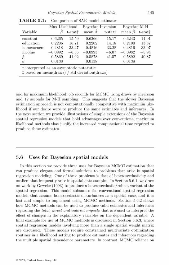
Bayesian Spatial Econometric Models 145
TABLE 5.1: Comparison of SAR model estimatesMax Likelihood Bayesian Inversion Bayesian M-H
Variable β t-stat† mean β t-stat‡ mean β t-stat‡constant 0.6265 15.59 0.6266 15.17 0.6243 14.91education 0.2206 16.71 0.2202 14.18 0.2190 13.87homeowners 0.4818 33.47 0.4816 33.28 0.4816 33.07income −0.0992 −6.35 −0.0993 −6.07 −0.0982 −5.94ρ 0.5869 41.92 0.5878 41.57 0.5892 40.87σ 0.0138 0.0138 0.0138
† interpreted as an asymptotic t-statistic‡ based on mean(draws) / std deviation(draws)
ond for maximum likelihood, 6.5 seconds for MCMC using draws by inversionand 12 seconds for M-H sampling. This suggests that the slower Bayesianestimation approach is not computationally competitive with maximum like-lihood if our desire were to produce the same estimates and inferences. Inthe next section we provide illustrations of simple extensions of the Bayesianspatial regression models that hold advantages over conventional maximumlikelihood methods that justify the increased computational time required toproduce these estimates.
5.6 Uses for Bayesian spatial models
In this section we provide three uses for Bayesian MCMC estimation thatcan produce elegant and formal solutions to problems that arise in spatialregression modeling. One of these problems is that of heteroscedasticity andoutliers that frequently arise in spatial data samples. In Section 5.6.1, we drawon work by Geweke (1993) to produce a heteroscedastic/robust variant of thespatial regression. This model subsumes the conventional spatial regressionmodels that assume homoscedastic disturbances as a special case, and it isfast and simple to implement using MCMC methods. Section 5.6.2 showshow MCMC methods can be used to produce valid estimates and inferencesregarding the total, direct and indirect impacts that are used to interpret theeffect of changes in the explanatory variables on the dependent variable. Afinal example for use of MCMC methods is discussed in Section 5.6.3, wherespatial regression models involving more than a single spatial weight matrixare discussed. These models require constrained multivariate optimizationroutines in a likelihood setting to produce estimates and inferences regardingthe multiple spatial dependence parameters. In contrast, MCMC reliance on
© 2009 by Taylor & Francis Group, LLC
146 Introduction to Spatial Econometrics
conditional distributions considerably simplifies estimation of these models.
5.6.1 Robust heteroscedastic spatial regression
One concrete illustration of the extensible nature of the MCMC estimationmethod is to extend our simple SAR model to include variance scalars thatcan accommodate heteroscedastic disturbances and/or outliers.
This type of prior information was introduced by Albert and Chib (1993)for the ordinary probit model and Geweke (1993) for a least-squares model.The prior pertains to assumed homoscedastic versus heteroscedastic distur-bances. A set of variance scalars (v1, v2, . . . , vn), is introduced that repre-sent unknown parameters that need to be estimated. This allows us to as-sume ε ∼ N(0, σ2V ), where V is a diagonal matrix containing parameters(v1, v2, . . . , vn). The prior distribution for the vi terms takes the form of a setof n iid χ2(r)/r distributions, where r represents the single parameter of theχ2 distribution. This allows us to estimate the additional n variance scalingparameters vi by adding only a single parameter r, to our model. Use of a flex-ible family of distributions that is controlled by a single parameter such as r tospecify a prior distribution is a common Bayesian approach. The parameterr that controls this family of prior distributions is labeled a hyperparameter.The notion here is that changes in this single parameter can potentially exerta great deal of influence on the nature of the prior distribution assigned tothe model parameters it controls.
The specifics regarding the prior assigned to the vi variance scaling param-eters can be motivated by noting that a prior mean of unity will be assignedand a prior variance equal to 2/r. This implies that as the hyperparameter r isassigned very large values, the prior variance becomes very small leading thevariance scaling parameters vi to approach their prior mean values of unity.This results in a prior specification that: V = In, the traditional assumptionof constant variance across our observations or regions/points located in space.On the other hand, a small value assigned to the hyperparameter r will leadto a skewed prior distribution assigned to the variance scalar parameters vi.The large prior variance leads to skew in the χ2 prior distributions assignedto each variance scalar which will allow the estimates and posterior means forthese parameters to deviate greatly from their prior mean values of unity.
Large values for the variance scalars vi are associated with outliers or obser-vations containing large variances. These observations will be down-weightedas in the case of generalized least-squares where large variances result in lessweight assigned to an observation. In the context of spatial modeling, outliersor aberrant observations can arise due to enclave effects, where a particu-lar area exhibits divergent behavior from nearby areas. As an example, wemight see different crime rates in a “gated community” than in surroundingneighborhoods. Geweke (1993) shows that this approach to modeling the dis-turbances is equivalent to a model that assumes a Student-t prior distributionfor the errors. We note that this type of distribution has frequently been used
© 2009 by Taylor & Francis Group, LLC
Bayesian Spatial Econometric Models 147
to deal with sample data containing outliers (Lange, Little and Taylor, 1989).A formal statement of the Bayesian heteroscedastic SAR model is shown in
(5.32), where we have added an independent normal and inverse-gamma priorfor β and σ2, and a uniform prior for ρ. This represents a departure from ourprevious use of the NIG prior for the parameters β and σ2. This type of prioris generally considered more flexible, but does not have the advantage of beingconjugate. Since we are relying on MCMC estimation, use of a conjugate prioris no longer important. These priors are in addition to the chi-squared priorfor variance scalars, but as noted they are unlikely to exert much impact onthe resulting estimates and inferences in large samples. As before, the priordistributions are indicated using π().
y = ρWy +Xβ + ε
ε ∼ N(0, σ2V )Vii = vi, i = 1, . . . , n, Vij = 0, i �= j
π(β) ∼ N(c, T )π(r/vi) ∼ iid χ2(r), i = 1, . . . , nπ(σ2) ∼ IG(a, b)π(ρ) ∼ U(1/λmin, 1/λmax) (5.32)
We need the conditional posterior distributions for the parameters β, σ, andρ as well as the variance scalars vi, i = 1, . . . , n in this model to implementour MCMC sampling scheme. The conditional distribution for β takes theform of a multivariate normal shown in (5.33), which is a simple GLS variantof our previous expression, where the variance is known. This arises becausewe can condition on all other parameters in the model, including the diagonalmatrix of variance scalars V .
p(β|ρ, σ, V ) ∝ N(c∗, T ∗) (5.33)c∗ = (X ′V −1X + σ2T−1)−1(X ′V −1(In − ρW )y + σ2T−1c)T ∗ = σ2(X ′V −1X + σ2T−1)−1
This illustrates an attractive feature of the MCMC method. Working withconditional posterior distributions greatly simplifies the calculations requiredto extend a basic model. If we have already developed computational code toimplement a simpler homoscedastic model where V = In, the modificationsrequired to implement this model are minor.
The expression needed to produce a draw from the conditional posteriordistribution of σ2 takes the form in (5.34). Using the relationship notedearlier involving the residuals, we see that we have a type of GLS expression,where the non-constant variance reflected by the diagonal matrix V can beassumed known.
© 2009 by Taylor & Francis Group, LLC
148 Introduction to Spatial Econometrics
p(σ2|β, ρ, V ) ∝ IG(a∗, b∗) (5.34)a∗ = a+ n/2b∗ = (2b+ e′V −1e)/2e = Ay −Xβ
A = In − ρW
The expression needed to produce draws for the parameter ρ takes theunknown distributional form shown in (5.35) (LeSage, 1997). This meanswe can still rely on either our numerical integration followed by a draw viainversion or the M-H approach.
p(ρ|β, σ2, V ) ∝ |A| exp(− 1
2σ2e′V −1e
)(5.35)
Geweke (1993) shows that the conditional distribution of V given the otherparameters is proportional to a chi-square density with r + 1 degrees of free-dom. Specifically, we can express the conditional posterior of each vi as in(5.36), where v−i = (v1, . . . , vi−1, vi+1, . . . , vn) for each i. That is, we sampleeach variance scalar conditional on all others. The term ei represents the ithelement of the vector e = Ay −Xβ.
p(e2i + r
vi|β, ρ, σ2, v−i) ∝ χ2(r + 1) (5.36)
We summarize by noting that estimation of this extended model requiresadding a single conditional distribution for the new variance scalar parametersvi introduced in the model to our MCMC sampling scheme. In addition,we made minor adjustments to the conditional posterior distributions for theother parameters in the model to reflect the presence of these new parameters.These adjustments would require only minor changes to any computationalcode already developed for the simpler model from Section 5.4.
A point to note is that introducing heteroscedastic disturbances in the con-text of a model estimated using maximum likelihood was proposed by Anselin(1988). However, that approach requires the modeler to specify a functionalform as well as variables thought to model the non-constant variance overspace. The approach introduced here does not require this additional modelfor the non-constant variance. In addition to automatically detecting and ad-justing for non-constant variances, the MCMC method will also detect andautomatically down-weight outliers or aberrant observations.
From a practitioner’s viewpoint, it would seem prudent to use this methodwith a prior hyperparameter setting of r = 4. This prior is consistent with aprior belief in heteroscedasticity, or non-constant variance as well as outliers.If the sample data does not contain these problems, the resulting posteriorestimates for the variance scalar parameters vi will take values near unity. A
© 2009 by Taylor & Francis Group, LLC
Bayesian Spatial Econometric Models 149
plot of the posterior mean of the variance scalar parameters can serve as adiagnostic for outliers or heteroscedasticity. A map of the posterior mean vivalues can be used to locate regions/observations with high and low varianceas well as outliers.
It makes little sense to use this model with a large prior value assignedto the hyperparameter r. This reflects a prior belief in homoscedasticity. Ifa practitioner is confident regarding homoscedastic disturbances, then maxi-mum likelihood estimates are much faster and easier to produce.
5.6.2 Spatial effects estimates
Gelfand et al. (1990) point out that the draws from MCMC sampling canbe used to produce posterior distributions for functions of the parameters thatare of interest. This makes testing complicated parameter relationships quitesimple. For example, suppose we are interested in the hypothesis: γ = α ·β <1, where α, β are parameters in a model estimated with MCMC sampling. Wecan simply multiply the m draws for α(j) and β(j), j = 1, . . . ,m, to produceγ(j), j = 1, . . . ,m. The posterior distribution of γ = α · β can be used to findthe posterior probability that γ < 1. This would be equal to the proportionof all draws in the vector γ that take values less than unity. If we find that9,750 draws from a sample of 10,000 are less than unity, then the probabilityis 97.5%. Of course means, modes and standard deviations could also beconstructed using the draws for γ.
If we are interested in conducting inference regarding the summary mea-sures of the cumulative total, direct and indirect impacts associated withchanges in the explanatory variables described in Chapter 2, we can con-struct these during the MCMC sampling process. On each pass through thesampler, we can use the current set of draws to produce a total and directimpact, as well as the indirect impact by subtracting the direct from the to-tal effect. Saving these draws allows us to use these to construct the entireposterior distribution for the three types of impacts that arise from changingthe explanatory variables X in the model.
In Chapter 2 we established the notion that each explanatory variable r hasa multiplier impact on y that could be expressed as: y =
∑pr=1 Sr(W )xr+ . . .,
where the multiplier term Sr(W ) takes different forms for the various membersof the family of spatial models. For example, for the SDM model: y =ρWy +Xβ +WXθ + ε, we have Sr(W ) = (In − ρW )−1(Inβr +Wθr).
It should be easy to see that the sampled parameters β, θ, ρ could be directlyentered into Sr(W ) on each pass through the MCMC sampling loop. Thiscould be used to produce MCMC samples of the summary measures of the(average) cumulative direct impacts shown in (5.37), cumulative total impactsin (5.38) and cumulative indirect impacts in (5.39).
© 2009 by Taylor & Francis Group, LLC
150 Introduction to Spatial Econometrics
direct: Mr(D) = n−1tr(Sr(W )) (5.37)total: Mr(T ) = n−1ι′nSr(W )ιn (5.38)
indirect: Mr(I) = Mr(T ) − Mr(D) (5.39)
However, a more computationally astute approach would be to use theefficient trace computations set forth in Chapter 4 in conjunction with theMCMC draws. Use of the MCMC draws for problems involving small samplesmight produce a more accurate posterior parameter distribution than wouldarise from using maximum likelihood estimates to simulate from a multivariatenormal distribution. This could occur because in small samples parametersmay exhibit asymmetry or heavy tailed distributions that deviate slightly fromnormality.
5.6.3 Models with multiple weight matrices
We discuss how MCMC sampling can be used to estimate models such as theSAC from Chapter 2, that include more than a single spatial weight matrix.For models that contain numerous weight matrices and associated spatialdependence parameters, MCMC sampling from the conditional distributionsleads to an important simplification.
The SAC model takes the form in (5.40) with the associated likelihoodconcentrated for the parameters β, σ2 shown in (5.41).
y = ρWy +Xβ + u
u = λMu+ ε (5.40)ε ∼ N(0, σ2In)
p(y|β, σ, ρ, λ) ∝ |A||B|exp(− 1
2σ2(BAy −BXβ)′(BAy −BXβ)
)(5.41)
A = In − ρW
B = In − λM
Maximizing the log of the likelihood function in (5.41) requires that wecalculate two log-determinants |A| and |B|, and the optimization probleminvolves solving a two-dimensional constrained optimization problem. Theconstraints are imposed to bound the spatial dependence parameters to theirrespective ranges based on the minimum and maximum eigenvalues of thespatial weight matrices W and M . This is not an extremely difficult opti-mization problem given current computational hardware and software, alongwith the efficient methods for computing log-determinants of sparse matricesdescribed in Chapter 4.
The advantage of MCMC sampling the model from (5.40) is that the con-ditional distributions for ρ and λ take the forms shown in (5.42) and (5.43).
© 2009 by Taylor & Francis Group, LLC
Bayesian Spatial Econometric Models 151
p(ρ|β, σ, λ) ∝ p(ρ, λ, β, σ|y)p(λ, β, σ|y) (5.42)
∝ |A||B(λc)|exp(− 1
2σ2(BAy − BXβ)′(BAy − BXβ)
)p(λ|β, σ, ρ) ∝ p(ρ, λ, β, σ|y)
p(ρ, β, σ|y) (5.43)
∝ |A(ρc)||B|exp(− 1
2σ2(BAy −BXβ)′(BAy −BXβ)
)We note that when sampling for the parameter ρ, we rely on the currentvalue/draw for λ in |B|, which we denote |B(λc)|, and B(λc) = B. Similarly,when sampling for the parameter λ we use the current value of ρ in |A| and A,with similar notation. An implication of this is that we could still carry outour univariate numerical integration scheme to find a normalizing constantand produce a CDF from which to draw by inversion. Similarly, carryingout Metropolis-Hastings sampling for the parameter ρ is no more complicatedthan in the case of a model where the additional spatial dependence parameterλ does not exist. We can produce candidate values for the parameter ρ from anormal random-walk proposal density using the same procedure as describedin section 5.3.2.
One can envision richer models that increase the number of spatial weightmatrices. For example, a model similar to the model in (5.44) can be foundin Lacombe (2004), where a sample of counties on borders of states was usedto carry out an analysis of the state-level impact of public policy differencesbetween states. The spatial weight matrix W was used to extract neighboringcounties across the border in another state, whereas the weight matrix V wasused to include dependence on neighboring counties within the same state.
y = ρWy + γV y +Xβ + u
u = λMu+ ε (5.44)ε ∼ N(0, σ2In)
The likelihood for this model shown in (5.45) involves the log-determinantterms: |A| = |In− ρW − γV | and |In−λM |. Maximum likelihood estimationinvolves three-dimensional optimization of the concentrated likelihood withrespect to the parameters β and σ2 to produce estimates for the parametersρ, γ and λ. This requires computing the log-determinant term: |In − ρW −γV |, over a two-dimensional grid of values for the parameters ρ and γ (seeChapter 4). There is also the log-determinant term |B| = |In − λM | definedin (5.45) that arises from the spatial autoregressive disturbance process, aswell as the stability constraint ρ+γ < 1, which must be applied when solvingthe optimization problem.
© 2009 by Taylor & Francis Group, LLC
152 Introduction to Spatial Econometrics
p(y|β, σ, ρ) = (2πσ2)−n2 |A| |B| exp
(− 1
2σ2(BAy −BXβ)′(BAy −BXβ)
)A = |In − ρW − γV |B = |In − λM | (5.45)
MCMC estimation of this model allows us to fix the log-determinant Abased on the current values of the parameters ρ and γ when sampling forthe parameter λ from its conditional distribution. Similarly, we can fix thelog-determinant B when sampling for the parameters ρ and γ. The stabil-ity restriction can be imposed using rejection sampling. This simply involvesrejecting Metropolis-Hastings candidate values that violate the stability re-striction. A count of the number of times these rejections occur during thesampling draws provides a posterior probability measure for consistency ofthe sample data with the stability restriction.
5.7 Chapter summary
Application of traditional Bayesian methods to estimation of spatial au-toregressive models requires simple univariate numerical integration of theposterior distribution with respect to the parameter ρ over a closed inter-val. In contrast, recent advances in the area of Markov Chain Monte Carlo(MCMC) estimation allow Bayesian estimation of spatial autoregressive mod-els as well as a host of useful variants on these models without the need toresort to numerical integration. We demonstrated that Bayesian methods inconjunction with MCMC estimation allow the basic family of spatial autore-gressive models to be implemented in the usual case where disturbances arenormally distributed with constant variances.
The greatest value of Bayesian MCMC methods lies in their ability to ex-tend the basic spatial regression models to accommodate situations where thesample data exhibit outliers or heteroscedasticity. These methods are alsouseful for generating spatial impact estimates which take the form of func-tions of the model parameters. These functions can be used to determine theimpact of changes in the explanatory variables of the model on the dependentvariable. Use of MCMC draws in the functions allows a simple approach toinference regarding the dispersion of the impacts. Finally, MCMC methods al-low estimation of models involving more than a single weight matrix, withoutresort to multivariate constrained optimization routines that are required formaximum likelihood estimation of these models. We will see other examplesof places where MCMC methods can be applied to spatial regression modelsin other chapters.
© 2009 by Taylor & Francis Group, LLC

Bayesian Spatial Econometric Models 153
A final point regarding the Bayesian methodology is that inference pro-ceeds identically for all Bayesian models implemented with MCMC methods.The entire posterior distribution is available for all parameters in the modelallowing means, medians, or modes to be used as point estimates, and mea-sures of dispersion are easily constructed. This is in contrast to cases wherealternatives to maximum likelihood estimation such as generalized method ofmoments are adopted to solve difficult spatial econometric problems. Here,inference may require adopting an alternative paradigm, or reliance on asymp-totic approximations whose statistical operational characteristics are not well-understood.
© 2009 by Taylor & Francis Group, LLC
Chapter 6
Model Comparison
This chapter describes model comparison procedures that allow practition-ers to draw inferences regarding various aspects of spatial econometric modelspecifications. We focus on comparison of: 1) spatial versus non-spatial mod-els, 2) models based on alternative spatial weight structures, and 3) modelsconstructed using different sets of candidate explanatory variables.
A variety of strategies and statistical methods for comparing alternativemodel specifications are introduced in Section 6.1, with an applied illustrationof these ideas provided in Section 6.2. Section 6.3 turns attention to Bayesianapproaches to model comparison which provide a unified approach to thevarious types of model comparison issues that confront practitioners. A seriesof applied illustrations for these methods are provided in each section.
6.1 Comparison of spatial and non-spatial models
When maximum likelihood estimation is used for spatial regression models,inference on the spatial dependence parameter ρ can be based on a Wald testconstructed using an asymptotic t-test from the estimated variance-covariancematrix, or a likelihood ratio test. These tests for spatial dependence versusthe null hypothesis of no dependence require maximum likelihood estimationof the spatial model representing the alternative to the null hypothesis of nospatial dependence.
Since maximum likelihood estimation was cumbersome in the past, thereis a great deal of literature on Lagrange Multiplier test statistics that requireonly estimation of the non-spatial model associated with the null hypothesis.For example, Burridge (1980) proposed an LM test for least-squares againstthe alternative SEM model taking the form shown in (6.1), where only least-squares residuals denoted by e, and a spatial weight matrix W are needed.The LM statistic in (6.1) follows an asymptotic χ2(1) distribution.
LM = [e′We/(e′e/n)]2/tr(W 2 +W ′W ) (6.1)
This statistic is related to an I-statistic proposed by Moran (1948), whichhas received a great deal of attention in the literature. This statistic also
155© 2009 by Taylor & Francis Group, LLC
156 Introduction to Spatial Econometrics
involves only use of the residuals from least-squares. Anselin (1988b) proposedLM tests for least-squares versus the SAR model, where again the appeal ofthese tests was that they did not require maximum likelihood estimation ofthe spatial model.
Given the current availability of software that makes estimation of the fam-ily of spatial regression models relatively simple and computationally fast, it iseasy to test for spatial dependence using inference on the spatial dependenceparameter ρ. This can be based on a t-test (constructed using the estimatedvariance-covariance matrix) for the null hypothesis that ρ = 0, or based on alikelihood ratio test that compares the spatial and non-spatial models.
An example of this would be comparison of a non-spatial regression model,which is nested within the spatial SAR model. Comparison of the non-spatialand spatial SAR model likelihoods, or use of a t-statistic on the spatial depen-dence parameter would allow one to draw an inference regarding the signifi-cance of spatial dependence in the dependent variable. A complication arisesbecause this test ignores possible spatial dependence in the disturbances, sinceit conditions on a model specification involving spatial dependence in the de-pendent variable. It is also the case that a comparison of an ordinary non-spatial regression versus SEM models would ignore spatial dependence in thedependent variable, focusing only on dependence in the disturbances of themodel. Joint tests that have power against the other alternative have beenproposed by Anselin (1988b), as well as tests that are reported to be robustto misspecification involving the alternative form of dependence by Anselin,Bera, Florax and Yoon (1996).
This same issue arises when attempting to ascertain the appropriate modelspecification based on a comparison of likelihood function values, since SARmodels ignore error dependence and SEM models do not account for spatialdependence in the dependent variable. The non-nested nature of these modelsgreatly complicates formal testing for both spatial dependence, as well as anappropriate model specification.
However, as indicated in Chapter 2, the SDM model nests models involvingdependence in both the disturbances as well as the dependent variable. Thereis too much emphasis in the spatial econometrics literature on use of statisticaltesting procedures to infer the appropriate model specification, and much ofthis literature ignores the SDM model. We make a number of observationsregarding the benefits and costs associated with alternative spatial regressionmodel specifications.
The cost of ignoring spatial dependence in the dependent variable is rel-atively high since biased estimates will result if this type of dependence isignored. In addition, ignoring this type of dependence will also lead to aninappropriate interpretation of the explanatory variable coefficients as rep-resenting partial derivative impacts arising from changes in the explanatoryvariables. In contrast, ignoring spatial dependence in the disturbances willlead to a loss of efficiency in the estimates. As samples become large, effi-ciency becomes less of a problem relative to bias. Spatial data availability
© 2009 by Taylor & Francis Group, LLC
Model Comparison 157
has increased dramatically for a number of reasons, including: increasingawareness of the need to consider variation in socio-economic relationshipsover space; improvements in geographical information system software andaccompanying computational advances in geo-referencing sample data usingpostal addresses; improved software for working with Census data sets; andUS government requirements that agencies make data available on the Inter-net. Because of this, efficiency of estimates may be of less concern as we beginanalyzing larger spatial data samples. There is still the problem that ignor-ing spatial dependence in the disturbances will lead to bias in the inferencesregarding dispersion of the estimates.
This line of reasoning suggests an asymmetric loss function for practition-ers interested in unbiased estimates, since the costs of ignoring spatial depen-dence in the dependent variable is more likely to produce biased estimatesthan ignoring dependence in the disturbances. Alternatively, the benefitsfrom accounting for dependence in the disturbances are increased efficiencyof the estimates, whereas those arising from proper modeling of dependencein the dependent variable are reductions in bias of the explanatory variablecoefficients, as well as improved efficiency.
In Chapter 2 we demonstrated that the presence of omitted variables in theSEM model will lead to the true data generating process being that associatedwith the SDM model. That is, use of the SDM model will help protect againstomitted variables bias. It was also shown that the SDM model nests bothspatial lag and spatial error models.
Finally, we note that inclusion of variables such as WX in the SDM modelwhen the true DGP is the SAR model that does not include these variableswill not lead to biased estimates for the explanatory variable parameters. Insituations where omitted variables lead to the presence of WX in the modelrelationship, use of the SAR model that excludes these variables leads toomitted variables bias in the coefficient estimates.
Putting these ideas together allows us to consider reciprocal misspecificationbias that can arise in the coefficient estimates from a costs versus benefitsperspective. We enumerate the implications for biased coefficient estimatesin the SEM, SAR, SDM and SAC models from a reciprocal misspecificationviewpoint below.1
1. For cases where the true DGP is the SEM model, involving only spa-tial dependence in the disturbances, the SAR, SAC and SDM modelswill still produce unbiased but inefficient coefficient estimates. Inferenceregarding dispersion of the explanatory variables based on the asymp-totic variance-covariance matrix for the SAR model will be mislead-
1We focus on the unbiasedness property of the coefficient estimates in our reciprocal mis-specification considerations. In the presence of biased coefficient estimates, we are lessconcerned about correct inferences regarding the dispersion of the biased coefficient esti-mates.
© 2009 by Taylor & Francis Group, LLC
158 Introduction to Spatial Econometrics
ing, since error dependence is ignored when constructing the variance-covariance matrix. Error dependence is taken into account in the asymp-totic variance-covariance matrix of the SDM and SAC models.
2. When the true DGP is the SAR model that includes spatial lag depen-dence, the SEM model would produce biased coefficient estimates, theSAR, SDM and SAC models would produce unbiased estimates, withmeasures of coefficient dispersion for the SDM and SAC models beingcorrect. Recall that including variables such as WX in the model whentheir coefficients are zero does not produce bias in the explanatory vari-ables estimates. Similarly, incorporating a model for spatial dependencein the disturbances where the dependence parameter is truly zero willnot have an adverse impact on the SAC estimates for sufficiently largesamples.
3. When the true DGP is the SDM model that includes both spatial lag de-pendence as well as spatial lags of the explanatory variables, the SEM,SAR and SAC coefficient estimates will suffer from omitted variablesbias, since these models do not include the spatially lagged explanatoryvariables WX . The SEM model will suffer additional bias due to ex-clusion of the spatial lag of the dependent variable. The correctness ofinference regarding the biased coefficient estimates for the SEM, SARand SAC models becomes a moot issue here.
4. When the true DGP is the SAC model that includes both spatial lagand spatial error dependence, the SAR and SDM models will produceunbiased coefficient estimates, while the SEM model coefficients willbe biased because this model ignores the spatial lag of the dependentvariable. Incorrect inferences regarding dispersion of the estimates arelikely to arise for the SAR model from ignoring spatial dependence inthe disturbances. The SDM model does not ignore spatial dependencein the disturbances, but implies a different type of specification for errordependence from that in the true SAC DGP. The impact on inferenceregarding dispersion of the unbiased SDM coefficients in this type ofsituation is an issue that needs further exploration.
The conclusion we draw is that the SDM is the only model that will pro-duce unbiased coefficient estimates under all four possible data generatingprocesses. Inference about the dispersion of the unbiased SDM coefficient es-timates in cases 1, 2 and 3 above will be correct, whereas case 4 is an issuethat requires exploration.
We also reiterate our point from Chapter 2 that beginning with a DGPbased on simple error dependence, the presence of omitted variables will leadto a model specification that conforms to the SDM. Since omitted variablesare likely when dealing with regional data samples, this is another motivationfor use of the SDM model.
© 2009 by Taylor & Francis Group, LLC
Model Comparison 159
6.2 An applied example of model comparison
There is a great deal of literature that examines regional production fromthe standpoint of the new economic geography (Duranton and Puga, 2001;Autant-Bernard, 2001; Autant-Bernard, Mairesse and Massard, 2007; Parentand LeSage, 2008). A question of interest is the role of regional differences intechnology on production, Q. This is often explored using a constant returnsregional production function shown in (6.2), where A represents technology,K capital and L labor inputs, and the shares parameter ψ is such that wehave constant returns to scale.
Q = AK(1−ψ)Lψ (6.2)
A total factor productivity relationship can be derived from the Cobb-Douglas production function as shown in (6.3).
lnQ = ψlnL+ (1 − ψ)lnK + lnAlnQ− ψlnL− (1 − ψ)lnK = lnA
tfp = lnA (6.3)
Our interest centers on whether the regional stock of patents can play therole of the technology variable A in (6.3). Intuitively, the stock of corporatepatents in each region should reflect a proxy for technology used in regionalproduction.
Patent stocks which we label A act as an empirical proxy for technology,but these are unlikely to capture the true technology available to regions.We posit the existence of unmeasured technology, which we label A∗ that isexcluded from the (log) linear relationship in (6.3). It has become a stylizedfact that empirical measures of regional technical knowledge A such as patentapplications, educational attainment, expenditures or employment in researchand development etc., exhibit spatial dependence (Autant-Bernard, Mairesseand Massard, 2007; Parent and LeSage, 2008). If both the measured variableA included in the empirical relationship (6.3) and the unmeasured excludedvariable A∗ exhibit spatial dependence, then our development in Chapter 2indicates that a spatial regression relationship will result.
Specifically, let the spatial autoregressive processes in (6.4) and (6.5) governspatial formation of technical knowledge stocks a = lnA and a∗ = lnA∗. Then × 1 vector a reflects (logged) cross-sectional observations on regional tech-nology in a sample of n regions, and we have introduced zero mean, constantvariance disturbance terms u, v, ε, along with an n× n spatial weight matrixW reflecting the connectivity structure of the regions. The scalar parametersφ and ρ reflect the strength of spatial dependence in a and a∗.
© 2009 by Taylor & Francis Group, LLC
160 Introduction to Spatial Econometrics
a = φWa+ u (6.4)a∗ = ρWa∗ + v (6.5)v = uγ + ε (6.6)u ∼ N(0, σ2
uIn)v ∼ N(0, σ2
vIn)ε ∼ N(0, σ2
εIn)
The relationship in (6.6) reflects simple (Pearson) correlation between shocks(u, v) to technology stocks a and a∗ when the scalar parameter γ �= 0. Theparticular type of spatial regression that results will depend on whether thereis correlation between the shocks (γ �= 0), or no correlation (γ = 0).
If we begin with the relationship in (6.7), where we use y to denote tfpwhich is logged, and use the definitions in (6.4) to (6.6), we arrive at (6.8).2
y = βa+ a∗ (6.7)y = ρWy + a(β + γ) +Wa(−ρβ − φγ) + ε (6.8)y = ρWy + η1a+ η2Wa+ ε
The expression in (6.8) represents a spatial Durbin model (SDM). Thismodel subsumes the spatial error model SEM: (In−ρW )y = (In−ρW )aβ+ε,as a special case when the parameter γ = 0 indicating no correlation in shocksto measured and unmeasured technical knowledge, and when the restrictionη2 = −ρη1 is true. A simple likelihood-ratio test of the SEM versus SDMmodel can be used to test the restriction η2 = −ρη1.
Another way to view the condition γ = 0 is that the included variable a andexcluded variable a∗ are not correlated, since correlation between the shocks,u, v implies correlation between a and a∗. In the trivial case of no correlation,the omitted variable a∗ does not exert bias on our model estimates, whichcan be seen from β + γ = β, when γ = 0. Conventional omitted variablestreatment considers the non-trivial case where correlation exists between theincluded and excluded variables so that γ �= 0. A related point is that γ �= 0will lead to a rejection of the common factor restriction since the coefficientη1 = (β + γ) will not be equal to −ρη2 when γ �= 0, since η2 = (−ρβ − φγ).Intuitively, the only way an SEM model can be justified is if: 1) there are noomitted variables in the model or 2) if the included and excluded variables, aand a∗ do not exhibit correlation. An omitted variable that is correlated withthe stock of technical knowledge variable included in the model will lead to
2Without loss of generality we could include an intercept term in the model, but ignore thisterm in our discussion for simplicity.
© 2009 by Taylor & Francis Group, LLC
Model Comparison 161
a spatial regression model that must contain a spatial lag of the dependentvariable.
In addition to testing the SDM versus SEM models, we can also test forspatial dependence in measured knowledge stocks. For dependence in mea-sured knowledge stocks we can produce maximum likelihood estimates forthe spatial autoregressive model: a = φWa + u, and rely on an asymptotict-statistic to test whether the scalar parameter φ is different from zero.
This development provides a formal motivation for inclusion of what isknown as a “spatial lag” of the explanatory variable Wa in regression rela-tionships that seek to explore knowledge spillover effects in a spatial context.Our development arrives at a spatial regression specification as an econometricmeans of addressing omitted variables, unlike the theoretical models of Er-tur and Koch (2007) which directly include spatial dependence structures intheoretical economic relationships to arrive at the same result. Our startingpoint is a non-spatial theoretical relationship where included and excludedexplanatory variables exhibit spatial dependence, and the included and ex-cluded variables are correlated by virtue of common (correlated) shocks tothe spatial autoregressive processes governing these variables. In the eventthat the shocks are uncorrelated, we have an SEM model whereas correlationof the shocks leads to an SDM model as the spatial data generating process.
6.2.1 The data sample used
Following the same approach as in the application from Chapter 3, thedependent variable tfp in the relationship (6.3) was calculated using 2002real gross value added data (deflated by 1995 Euro prices) as the measure ofoutput Q, for a sample of 198 NUTS-2 European Union regions. The regionsrepresent the 15 pre-2004 EU member states. See Fisher, Scherngell andReisman (2008) for a complete description of the sample data.
Calculated regional shares of labor for each region during 2002 were usedalong with the assumption of constant returns to calculate regional tfp: lnQ−s � lnL − (1 − s) � lnK, where � represents the Haddamard (element-by-element) product of the n× 1 vector of regional shares and the n× 1 vectorsof regional labor L and capital K.
6.2.2 Comparing models with different weight matrices
To implement our model we require a spatial weight matrix W , which canbe constructed in a number of different ways. We could rely on a first-ordercontiguity weight matrix or a nearest-neighbor weight matrix based on mnearest-neighboring regions. Of course, we would row-normalize the weightmatrices for reasons set forth in Chapter 4.
There is the question of which weight matrix is most appropriate for ourmodel and sample data, and if we rely on a nearest-neighbor matrix W , thenumber m of neighbors to use must be specified. One approach to take would
© 2009 by Taylor & Francis Group, LLC
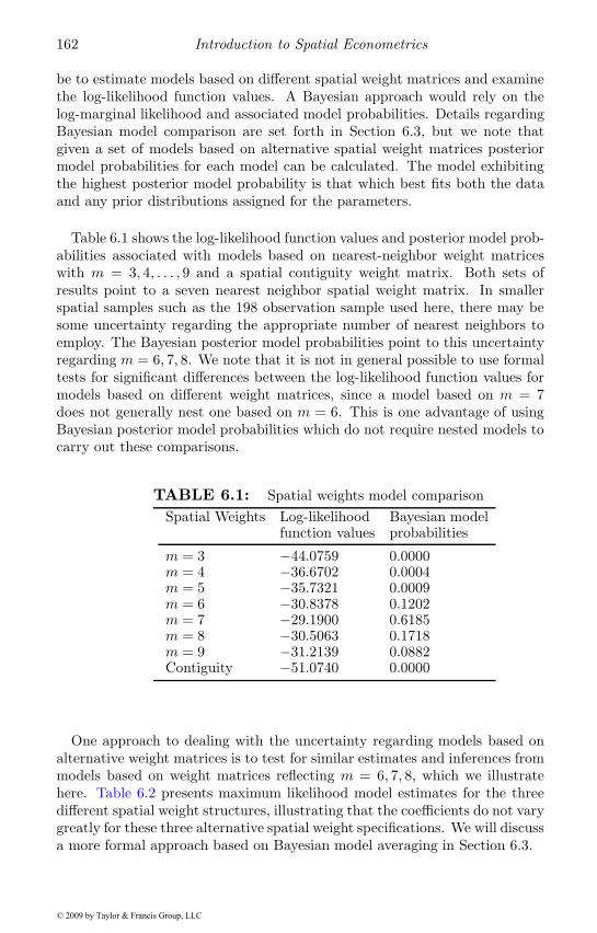
162 Introduction to Spatial Econometrics
be to estimate models based on different spatial weight matrices and examinethe log-likelihood function values. A Bayesian approach would rely on thelog-marginal likelihood and associated model probabilities. Details regardingBayesian model comparison are set forth in Section 6.3, but we note thatgiven a set of models based on alternative spatial weight matrices posteriormodel probabilities for each model can be calculated. The model exhibitingthe highest posterior model probability is that which best fits both the dataand any prior distributions assigned for the parameters.
Table 6.1 shows the log-likelihood function values and posterior model prob-abilities associated with models based on nearest-neighbor weight matriceswith m = 3, 4, . . . , 9 and a spatial contiguity weight matrix. Both sets ofresults point to a seven nearest neighbor spatial weight matrix. In smallerspatial samples such as the 198 observation sample used here, there may besome uncertainty regarding the appropriate number of nearest neighbors toemploy. The Bayesian posterior model probabilities point to this uncertaintyregarding m = 6, 7, 8. We note that it is not in general possible to use formaltests for significant differences between the log-likelihood function values formodels based on different weight matrices, since a model based on m = 7does not generally nest one based on m = 6. This is one advantage of usingBayesian posterior model probabilities which do not require nested models tocarry out these comparisons.
TABLE 6.1: Spatial weights model comparisonSpatial Weights Log-likelihood Bayesian model
function values probabilities
m = 3 −44.0759 0.0000m = 4 −36.6702 0.0004m = 5 −35.7321 0.0009m = 6 −30.8378 0.1202m = 7 −29.1900 0.6185m = 8 −30.5063 0.1718m = 9 −31.2139 0.0882Contiguity −51.0740 0.0000
One approach to dealing with the uncertainty regarding models based onalternative weight matrices is to test for similar estimates and inferences frommodels based on weight matrices reflecting m = 6, 7, 8, which we illustratehere. Table 6.2 presents maximum likelihood model estimates for the threedifferent spatial weight structures, illustrating that the coefficients do not varygreatly for these three alternative spatial weight specifications. We will discussa more formal approach based on Bayesian model averaging in Section 6.3.
© 2009 by Taylor & Francis Group, LLC
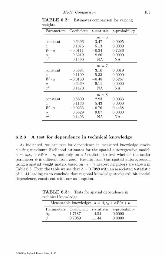
Model Comparison 163
TABLE 6.2: Estimates comparison for varyingweights
Parameters Coefficient t-statistic z-probability
m = 6constant 0.6396 3.47 0.0005a 0.1076 5.13 0.0000W · a −0.0111 −0.34 0.7286ρ 0.6219 8.86 0.0000σ2 0.1490 NA NA
m = 7constant 0.5684 3.10 0.0019a 0.1109 5.33 0.0000W · a −0.0160 −0.48 0.6267ρ 0.6469 9.11 0.0000σ2 0.1470 NA NA
m = 8constant 0.5600 2.93 0.0033a 0.1136 5.43 0.0000W · a −0.0255 −0.76 0.4458ρ 0.6629 9.07 0.0000σ2 0.1496 NA NA
6.2.3 A test for dependence in technical knowledge
As indicated, we can test for dependence in measured knowledge stocksa using maximum likelihood estimates for the spatial autoregressive model:a = β0ιn + φWa + u, and rely on a t-statistic to test whether the scalarparameter φ is different from zero. Results from this spatial autoregressionusing a spatial weight matrix based on m = 7 nearest neighbors are shown inTable 6.3. From the table we see that φ = 0.7089 with an associated t-statisticof 11.44 leading us to conclude that regional knowledge stocks exhibit spatialdependence, consistent with our assumption.
TABLE 6.3: Tests for spatial dependence intechnical knowledge
Measurable knowledge: a = β0ιn + φWa+ u
Parameters Coefficient t-statistic z-probabilityβ0 1.7187 4.54 0.0000φ 0.7089 11.44 0.0000
© 2009 by Taylor & Francis Group, LLC
164 Introduction to Spatial Econometrics
6.2.4 A test of the common factor restriction
The other test of interest is a comparison of the log-likelihood functionvalues from SDM versus SEM models. A likelihood ratio test provides a testof the common factor restriction: η2 = −ρη1. Given the results in Table 6.3showing spatial dependence in observed knowledge stocks, we would expect arejection of the SEM model in favor of the SDM model. The log-likelihoodwas −29.19 for the SDM model and −32.15 for the SEM model both basedon a seven nearest neighbor spatial weight matrix. This leads to a differenceof 2.96, and twice this difference in magnitude (5.92) represents a rejection ofthe SEM model in favor of the SDM model using the 95% critical value forχ2(1) which equals 3.84, but not at the 99% level where the critical value is6.635. The single degree of freedom reflects the single parameter restriction.
We can also test whether the more parsimonious SAR model that excludesthe spatial lag of knowledge stocks is more consistent with the sample datathan the SDM model using a likelihood ratio test. The log-likelihood for theSAR model was −34.42, leading to a difference with the SDM model of 5.23.Twice this difference (10.46) exceeds the 99% critical value of 6.635, allowingus to reject the SAR model in favor of the SDM model. Another way to testthis restriction is to consider the distribution for the non-linear parametercombination −ρ · η1 versus that for η2 based on the SDM model estimates.This can be accomplished using MCMC model estimation in conjunction withnon-informative prior distributions for the model parameters. This will leadto posterior estimates for these parameters that should exhibit the same dis-tribution as those from maximum likelihood estimation. Posterior means and95% and 99% upper and lower credible intervals were constructed using 5,000draws from MCMC estimation of the model, with the results shown in Ta-ble 6.4.
From the table we see that the posterior mean for the distribution of −ρη1 =−0.0687 is near the lower 0.95 credible interval for the parameter η2, consistentwith the likelihood ratio test results. As in the case of the likelihood ratiotest, the lower 0.99 credible interval for the parameter η2 (−0.0830) spansthe posterior mean value for −ρη1(−0.0687), precluding a 99% probabilityinference against the common factor restriction.
An important empirical implication is that if the included measures ofknowledge stocks are not correlated with excluded knowledge available to re-gions, then no spatial lag of the dependent variable is implied in the resultingmodel. In the case found here, there is strong but not overwhelming evidencethat included and excluded variables measuring regional knowledge stocks arecorrelated. This implies that a spatial lag of the dependent variable shouldbe used in the model, as well as a spatial lag of the explanatory variable Wa.Since omitting either of these from the empirical model will lead to biasedand inconsistent estimates for the parameters, it seems prudent to proceedusing the SDM model to examine the impact of knowledge stocks on y = tfp,the focus of this example.
© 2009 by Taylor & Francis Group, LLC
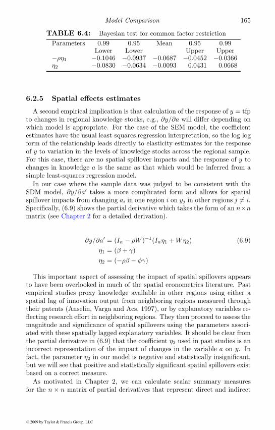
Model Comparison 165
TABLE 6.4: Bayesian test for common factor restrictionParameters 0.99 0.95 Mean 0.95 0.99
Lower Lower Upper Upper−ρη1 −0.1046 −0.0937 −0.0687 −0.0452 −0.0366η2 −0.0830 −0.0634 −0.0093 0.0431 0.0668
6.2.5 Spatial effects estimates
A second empirical implication is that calculation of the response of y = tfpto changes in regional knowledge stocks, e.g., ∂y/∂a will differ depending onwhich model is appropriate. For the case of the SEM model, the coefficientestimates have the usual least-squares regression interpretation, so the log-logform of the relationship leads directly to elasticity estimates for the responseof y to variation in the levels of knowledge stocks across the regional sample.For this case, there are no spatial spillover impacts and the response of y tochanges in knowledge a is the same as that which would be inferred from asimple least-squares regression model.
In our case where the sample data was judged to be consistent with theSDM model, ∂y/∂a′ takes a more complicated form and allows for spatialspillover impacts from changing ai in one region i on yj in other regions j �= i.Specifically, (6.9) shows the partial derivative which takes the form of an n×nmatrix (see Chapter 2 for a detailed derivation).
∂y/∂a′ = (In − ρW )−1(Inη1 +Wη2) (6.9)η1 = (β + γ)η2 = (−ρβ − φγ)
This important aspect of assessing the impact of spatial spillovers appearsto have been overlooked in much of the spatial econometrics literature. Pastempirical studies proxy knowledge available in other regions using either aspatial lag of innovation output from neighboring regions measured throughtheir patents (Anselin, Varga and Acs, 1997), or by explanatory variables re-flecting research effort in neighboring regions. They then proceed to assess themagnitude and significance of spatial spillovers using the parameters associ-ated with these spatially lagged explanatory variables. It should be clear fromthe partial derivative in (6.9) that the coefficient η2 used in past studies is anincorrect representation of the impact of changes in the variable a on y. Infact, the parameter η2 in our model is negative and statistically insignificant,but we will see that positive and statistically significant spatial spillovers existbased on a correct measure.
As motivated in Chapter 2, we can calculate scalar summary measuresfor the n × n matrix of partial derivatives that represent direct and indirect
© 2009 by Taylor & Francis Group, LLC
166 Introduction to Spatial Econometrics
(spatial spillover) impacts on the dependent variable (total factor productiv-ity) that arise from changing the explanatory variable a. The main diagonalof the matrix: (In − ρW )−1(Inη1 + Wη2) represents own partial derivatives(direct impacts), while the off-diagonal elements correspond to cross-partialderivatives (indirect impacts). These are averaged to produce scalar summarymeasures using the average of the main diagonal elements from the matrix andthe row- or column-sums of the matrix elements excluding the diagonal. Inaddition to these scalar measures of the mean direct and indirect impacts,we also construct measures of dispersion that can be used to draw inferencesregarding the statistical significance of the direct and indirect effects. Theseare based on simulating parameters from the normally distributed parametersη1, η2 and ρ, using the maximum likelihood estimates and associated variance-covariance matrix. The simulated draws are then used in the computationallyefficient formulas from Chapter 4 to calculate the implied distribution of thescalar summary measures.
An alternative to simulating draws based on maximum likelihood estimatesof the parameters and variance-covariance matrix is to rely on MCMC drawsfrom Bayesian estimation of the model using a diffuse prior for all modelparameters. This will produce results that are centered on the maximum like-lihood estimates which were reported in the applied illustration of Chapter 3.Table 6.5 presents these estimates based on 5,000 MCMC draws from Bayesianestimation of the model. The 5,000 draws were used to construct empiricalestimates of the lower and upper 0.95 and 0.99 credible intervals, reported inthe table. The scalar summaries shown in the table reflect cumulative impactsaggregated over space, since: (In − ρW )−1 = In + ρW + ρ2W 2 + . . ., we areexamining effects that fall on first-order neighbors (W ), second-order neigh-bors (W 2), and so on, cumulatively. The table reports impact estimates basedon alternative spatial weight matrices constructed using m = 6, 7, 8 nearestneighbors.
From the table, we see that the cumulative impact estimates are not verysensitive to the particular spatial weight matrix used, producing similar esti-mates and identical inferences regarding the significance of the impacts. Thedirect effects from changing knowledge stocks on regional total factor produc-tivity are positive and significantly different from zero using the 0.99 lowerand upper bounds. The indirect effects estimates are positive and differentfrom zero using the 0.95 bounds, but the 0.99 lower bound spans zero, sug-gesting we cannot be 99% confident that positive spatial spillovers exist. Themean indirect estimates for the case of m = 7 are around 1.5 times the sizeof the direct effects, suggesting a possible role for spatial spillovers arisingfrom regional patent stocks. As noted in Chapter 2, we interpret the effectsparameters in relation to movements from one steady-state equilibrium toanother. Given the log-transformations applied to both the dependent vari-able total factor productivity and the explanatory variable patent stocks, wecan interpret the effects magnitudes as elasticities. This implies that a 10%increase in the average stock of regional (corporate) patents would lead to a
© 2009 by Taylor & Francis Group, LLC
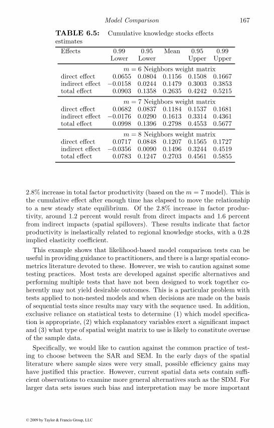
Model Comparison 167
TABLE 6.5: Cumulative knowledge stocks effectsestimates
Effects 0.99 0.95 Mean 0.95 0.99Lower Lower Upper Upper
m = 6 Neighbors weight matrixdirect effect 0.0655 0.0804 0.1156 0.1508 0.1667indirect effect −0.0158 0.0244 0.1479 0.3003 0.3853total effect 0.0903 0.1358 0.2635 0.4242 0.5215
m = 7 Neighbors weight matrixdirect effect 0.0682 0.0837 0.1184 0.1537 0.1681indirect effect −0.0176 0.0290 0.1613 0.3314 0.4361total effect 0.0998 0.1396 0.2798 0.4553 0.5677
m = 8 Neighbors weight matrixdirect effect 0.0717 0.0848 0.1207 0.1565 0.1727indirect effect −0.0356 0.0090 0.1496 0.3244 0.4519total effect 0.0783 0.1247 0.2703 0.4561 0.5855
2.8% increase in total factor productivity (based on the m = 7 model). This isthe cumulative effect after enough time has elapsed to move the relationshipto a new steady state equilibrium. Of the 2.8% increase in factor produc-tivity, around 1.2 percent would result from direct impacts and 1.6 percentfrom indirect impacts (spatial spillovers). These results indicate that factorproductivity is inelastically related to regional knowledge stocks, with a 0.28implied elasticity coefficient.
This example shows that likelihood-based model comparison tests can beuseful in providing guidance to practitioners, and there is a large spatial econo-metrics literature devoted to these. However, we wish to caution against sometesting practices. Most tests are developed against specific alternatives andperforming multiple tests that have not been designed to work together co-herently may not yield desirable outcomes. This is a particular problem withtests applied to non-nested models and when decisions are made on the basisof sequential tests since results may vary with the sequence used. In addition,exclusive reliance on statistical tests to determine (1) which model specifica-tion is appropriate, (2) which explanatory variables exert a significant impactand (3) what type of spatial weight matrix to use is likely to constitute overuseof the sample data.
Specifically, we would like to caution against the common practice of test-ing to choose between the SAR and SEM. In the early days of the spatialliterature where sample sizes were very small, possible efficiency gains mayhave justified this practice. However, current spatial data sets contain suffi-cient observations to examine more general alternatives such as the SDM. Forlarger data sets issues such bias and interpretation may be more important
© 2009 by Taylor & Francis Group, LLC
168 Introduction to Spatial Econometrics
than the variance of the estimates. We have argued that there are strongeconometric motivations for the SDM model, which subsumes the SAR andSEM models as a special case. Further, this model arises quite naturally inthe presence of omitted variables that are correlated with included variables.
In the next section we discuss Bayesian approaches to model comparison,which hold some advantages over likelihood-based methods. One advantage isthe ability to compare non-nested models that create difficulties for likelihood-ratio tests. A second advantage is that likelihood-based tests depend onthe quality of the point estimates used to evaluate the likelihood function.Bayesian model comparison methods integrate over the model parameters toproduce inferences regarding alternative models that are unconditional onspecific values taken by the model parameters.
6.3 Bayesian model comparison
Zellner (1971) sets forth the basic Bayesian theory behind model comparisonfor non-spatial regression models where a discrete set of m alternative modelsare under consideration. The approach involves specifying prior probabilitiesfor each model3 as well as prior distributions for the regression parameters.Posterior model probabilities are then calculated and used for inferences re-garding the consistency of alternative regression models with the sample dataand prior.
When we compare models based on alternative spatial weight structures,we typically have a small number m of alternative models, and the modelsdiffer only in terms of the type of spatial weight matrix used. A Bayesianapproach for comparing spatial regression models based on differing spatialweights is set forth in Section 6.3.1.
An alternative scenario arises when comparing models based on differentsets of explanatory variables. In these situations a small set of 15 candi-date explanatory variables will lead to 215 = 32, 768 possible models, anda larger set of 50 candidate variables results in 250 = 1.1259e + 015 mod-els. This makes it infeasible to calculate posterior model probabilities for thelarge number of possible models. A Markov Chain Monte Carlo model com-position methodology known as MC3 proposed by Madigan and York (1995)has gained popularity in the non-spatial regression literature (e.g. Dennison,Holmes, Mallick and Smith (2002); Fernandez, Ley, and Steel (2001)). Sincethe question of which explanatory variables are most important often arisesin applied regression modeling, the MC3 methods have gained popularity in
3The alternative models are often taken as equally likely, so each model is assigned thesame prior probability equal to 1/m, where m is the number of models under consideration.
© 2009 by Taylor & Francis Group, LLC
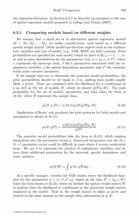
Model Comparison 169
the regression literature. In Section 6.3.2 we describe an extension to the caseof spatial regression models proposed in LeSage and Parent (2007).
6.3.1 Comparing models based on different weights
We assume that a small set of m alternative spatial regression modelsM = M1,M2, . . . ,Mm are under consideration, each based on a differentspatial weight matrix. Other model specification aspects such as the explana-tory variables and type of model, (e.g., SAR, SDM) are held constant. Priorprobabilities are specified for each model, which we label π(Mi), i = 1, . . . ,m,as well as prior distributions for the parameters π(η), η = (ρ, α, β, σ2), whereα represents the intercept term, β the k parameters associated with the ex-planatory variables, ρ the spatial dependence parameter and σ2 the constant,scalar noise variance parameter.
If the sample data are to determine the posterior model probabilities, theprior probabilities should be set equal to 1/m, making each model equallylikely a priori. These are combined with the likelihood for y conditional onη as well as the set of models M , which we denote p(D|η,M). The jointprobability for the set of models, parameters and data takes the form in(6.10), where D represents the sample data.
p(M,η,D) = π(M)π(η|M)p(D|η,M) (6.10)
Application of Bayes’ rule produces the joint posterior for both models andparameters as shown in (6.11).
p(M,η|D) =π(M)π(η|M)p(D|η,M)
p(D)(6.11)
The posterior model probabilities take the form in (6.12), which requiresintegration over the parameter vector η. Numerical integration over the (k +3)× 1 parameter vector could be difficult in cases where k is even moderatelylarge. We use k to represent the number of explanatory variables, and wehave three additional parameters for the intercept, spatial dependence andnoise variance.
p(M |D) =∫p(M,η|D)dη, (6.12)
As a specific example, consider the SAR model, where the likelihood func-tion for the parameters η = (α, β, σ2, ρ), based on the data D = {y, x,W}takes the form shown in (6.13), where we include the spatial weight matrix Wto indicate that the likelihood is conditional on the particular weight matrixemployed in the model. That is, the weight matrix is taken as given andtreated in the same manner as the sample data information in y,X .
© 2009 by Taylor & Francis Group, LLC
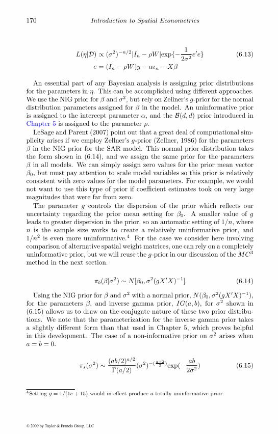
170 Introduction to Spatial Econometrics
L(η|D) ∝ (σ2)−n/2|In − ρW |exp{− 12σ2
e′e} (6.13)
e = (In − ρW )y − αιn −Xβ
An essential part of any Bayesian analysis is assigning prior distributionsfor the parameters in η. This can be accomplished using different approaches.We use the NIG prior for β and σ2, but rely on Zellner’s g-prior for the normaldistribution parameters assigned for β in the model. An uninformative prioris assigned to the intercept parameter α, and the B(d, d) prior introduced inChapter 5 is assigned to the parameter ρ.
LeSage and Parent (2007) point out that a great deal of computational sim-plicity arises if we employ Zellner’s g-prior (Zellner, 1986) for the parametersβ in the NIG prior for the SAR model. This normal prior distribution takesthe form shown in (6.14), and we assign the same prior for the parametersβ in all models. We can simply assign zero values for the prior mean vectorβ0, but must pay attention to scale model variables so this prior is relativelyconsistent with zero values for the model parameters. For example, we wouldnot want to use this type of prior if coefficient estimates took on very largemagnitudes that were far from zero.
The parameter g controls the dispersion of the prior which reflects ouruncertainty regarding the prior mean setting for β0. A smaller value of gleads to greater dispersion in the prior, so an automatic setting of 1/n, wheren is the sample size works to create a relatively uninformative prior, and1/n2 is even more uninformative.4 For the case we consider here involvingcomparison of alternative spatial weight matrices, one can rely on a completelyuninformative prior, but we will reuse the g-prior in our discussion of the MC3
method in the next section.
πb(β|σ2) ∼ N [β0, σ2(gX ′X)−1] (6.14)
Using the NIG prior for β and σ2 with a normal prior, N(β0, σ2(gX ′X)−1),
for the parameters β, and inverse gamma prior, IG(a, b), for σ2 shown in(6.15) allows us to draw on the conjugate nature of these two prior distribu-tions. We note that the parameterization for the inverse gamma prior takesa slightly different form than that used in Chapter 5, which proves helpfulin this development. The case of a non-informative prior on σ2 arises whena = b = 0.
πs(σ2) ∼ (ab/2)a/2
Γ(a/2)(σ2)−( a+2
2 )exp(− ab
2σ2) (6.15)
4Setting g = 1/(1e + 15) would in effect produce a totally uninformative prior.
© 2009 by Taylor & Francis Group, LLC
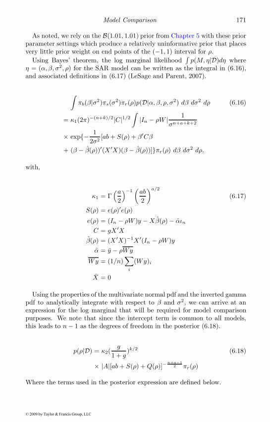
Model Comparison 171
As noted, we rely on the B(1.01, 1.01) prior from Chapter 5 with these priorparameter settings which produce a relatively uninformative prior that placesvery little prior weight on end points of the (−1, 1) interval for ρ.
Using Bayes’ theorem, the log marginal likelihood∫p(M,η|D)dη where
η = (α, β, σ2, ρ) for the SAR model can be written as the integral in (6.16),and associated definitions in (6.17) (LeSage and Parent, 2007).
∫πb(β|σ2)πs(σ2)πr(ρ)p(D|α, β, ρ, σ2) dβ dσ2 dρ (6.16)
= κ1(2π)−(n+k)/2|C|1/2∫
|In − ρW | 1σn+a+k+2
× exp{− 12σ2
[ab+ S(ρ) + β′Cβ
+ (β − β(ρ))′(X ′X)(β − β(ρ))]}πr(ρ) dβ dσ2 dρ,
with,
κ1 = Γ(a
2
)−1(ab
2
)a/2(6.17)
S(ρ) = e(ρ)′e(ρ)
e(ρ) = (In − ρW )y −Xβ(ρ) − αιn
C = gX ′Xβ(ρ) = (X ′X)−1X ′(In − ρW )yα = y − ρWy
Wy = (1/n)∑i
(Wy)i
X = 0
Using the properties of the multivariate normal pdf and the inverted gammapdf to analytically integrate with respect to β and σ2, we can arrive at anexpression for the log marginal that will be required for model comparisonpurposes. We note that since the intercept term is common to all models,this leads to n− 1 as the degrees of freedom in the posterior (6.18).
p(ρ|D) = κ2(g
1 + g)k/2 (6.18)
× |A|[ab+ S(ρ) +Q(ρ)]−n+a−1
2 πr(ρ)
Where the terms used in the posterior expression are defined below.
© 2009 by Taylor & Francis Group, LLC
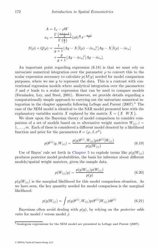
172 Introduction to Spatial Econometrics
A = In − ρW
κ2 =Γ(n+a−1
2
)Γ(a2
) (ab)a2 π−n−1
2
S(ρ) +Q(ρ) =1
g + 1[Ay −Xβ(ρ) − αιn]′[Ay −Xβ(ρ) − αιn]
+g
g + 1[Ay − αιn]′[Ay − αιn].
An important point regarding expression (6.18) is that we must rely onunivariate numerical integration over the parameter ρ to convert this to thescalar expression necessary to calculate p(M |y) needed for model comparisonpurposes, where we use y to represent the data. This is a contrast with con-ventional regression models where analytical integration over the parametersβ and σ leads to a scalar expression that can be used to compare models(Fernandez, Ley, and Steel, 2001). However, we provide details regarding acomputationally simple approach to carrying out the univariate numerical in-tegration in the chapter appendix following LeSage and Parent (2007).5 Thecase of the SDM model is identical to the SAR model presented here with theexplanatory variables matrix X replaced by the matrix X =
(X WX
).
We draw upon the Bayesian theory of model comparison to consider com-parison of a set of models based on m alternative weight matrices W(i), i =1, . . . ,m. Each of these is considered a different model denoted by a likelihoodfunction and prior for the parameters θ = (ρ, β, σ2).
p(θ(i)|y,W(i)) =p(y|θ(i),W(i))p(θ(i)|W(i))
p(y|W(i))(6.19)
Use of Bayes’ rule set forth in Chapter 5 to explode terms like p(y|W(i))produces posterior model probabilities, the basis for inference about differentmodels/spatial weight matrices, given the sample data.
p(W(i)|y) =p(y|W(i))p(W(i))
p(y)(6.20)
p(y|W(i)) is the marginal likelihood for this model comparison situation. Aswe have seen, the key quantity needed for model comparison is the marginallikelihood:
p(y|W(i)) =∫p(y|θ(i),W(i))p(θ(i)|W(i))dθ(i) (6.21)
Bayesians often avoid dealing with p(y), by relying on the posterior oddsratio for model i versus model j:
5Analogous expressions for the SEM model are presented in LeSage and Parent (2007).
© 2009 by Taylor & Francis Group, LLC
Model Comparison 173
POij =p(W(i)|y)p(W(j)|y) =
p(y|W(i))p(W(i))p(y|W(j))p(W(j))
(6.22)
A virtue of this approach is that posterior model probabilities or Bayes’factors can be used to compare non-nested models. This allows the methodto be used for comparing models based on: 1) different spatial weight matrices;2) different model specifications (including those that may not be members ofthe family of models set forth in Chapter 2; and 3) models based on differentsets of explanatory variables contained in the matrix X .
An issue that arises with this approach is the need to avoid a paradoxpointed out by Lindley (1957). He noted that when comparing models withdifferent numbers of parameters that rely on diffuse priors, the simpler modelis always favored over a more complex one, irrespective of the sample datainformation. An implication is that two models with an equal number ofparameters can be compared using diffuse priors, but for model comparisonsthat involve changes in the number of parameters, strategic priors must bedeveloped and used.
A strategic prior would recognize that flat priors can in fact be highlyinformative because assigning a diffuse prior over a parameter value assignsa large amount of prior weight to values of the parameter that are very largein absolute value terms. An implication is that there is no natural way toencode complete prior ignorance about parameters. A strategic prior in thecontext of model comparison involving alternative spatial weight matriceswould be one that explicitly recognizes the role that parameters and priorsplay in controlling model complexity. Given this, we could explore how priorsettings impact posterior model selection regarding the alternative spatialweight matrices.
For the case of homoscedastic disturbances in the SAR and SEM spatialregression models from Chapter 2, we have seen that we can analytically inte-grate out the parameters β and σ to arrive at an expression for the marginallikelihood that depends only on the parameter ρ. This is the only prior distri-bution we need be concerned with, since our comparison of models based ondifferent weight matrices does not depend on the parameters β and σ, becausethese have been integrated out. Hepple (1995b) provides expressions for thelog-marginal likelihood when non-informative priors are used for a number ofspatial regression models including the SAR and SEM.
6.3.2 Comparing models based on different variables
A large literature on Bayesian model averaging over alternative linear re-gression models containing differing explanatory variables exists (Fernandez,Ley, and Steel, 2001). The Markov Chain Monte Carlo model composition(MC3) approach introduced in Madigan and York (1995) is set forth here forthe case of spatial regression models. For a regression model with k possible
© 2009 by Taylor & Francis Group, LLC
174 Introduction to Spatial Econometrics
explanatory variables, there are 2k possible ways to select regressors to beincluded or excluded from the model. For k = 15, we have 32,768 possiblemodels, ruling out computation of the log-marginal for all possible models asimpractical.
The motivation for this literature is the classic trade-off between attempt-ing to include a sufficient number of explanatory variables in our models toovercome potential omitted variables bias and inclusion of redundant vari-ables that decrease precision of the estimates. It is precisely this trade-offthat model averaging seeks to address.
TheMC3 method of Madigan and York (1995) devises a strategic stochasticMarkov chain process that can move through the potentially large model spaceand sample regions of high posterior support. This eliminates the need toconsider all models by constructing a sampler that explores relevant parts ofthe very large model space. If we let M denote the current model state ofthe chain, models are proposed using a neighborhood, nbd(M) which consistsof the model M itself along with models containing either one more variable(labeled a ‘birth step’), or one less variable (a ‘death step’) than M . Atransition matrix, q, is defined by setting q(M → M ′) = 0 for all M ′ �∈nbd(M) and q(M → M ′) constant for all M ′ ∈ nbd(M). The proposedmodel M ′ is compared to the current model state M using the acceptanceprobability shown in (6.23).
min[1,p(M ′|y)p(M |y)
](6.23)
Use of univariate numerical integration methods described in the chapterappendix allows us to construct a Metropolis-Hastings sampling scheme thatimplements the MC3 method. A vector of the log-marginal values for thecurrent model M is stored during sampling along with a vector for the pro-posed model M ′. These are then scaled and integrated to produce the ratiop(M ′|y)/p(M |y) in (6.23) that determines acceptance or rejection of the pro-posed model. In contrast to conventional regression models, there is a needto store log-marginal density vectors for each unique model found during theMCMC sampling to calculate posterior model probabilities over the set of allunique models visited by the sampler.
Although the use of birth and death processes in the context of Metropolis-Hastings sampling will theoretically produce samples from the correct pos-terior, Richardson and Green (1997) among others advocate incorporating a“move step” in addition to the birth and death steps into the algorithm. Werely on this approach as there is evidence that combining these move stepsimproves convergence of the sampling process (Dennison, Holmes, Mallickand Smith, 2002; Richardson and Green, 1997). The move step takes theform of replacing a randomly chosen single variable in the current explana-tory variables matrix with a randomly chosen variable not currently in themodel. Specifically, we might propose a model with one less explanatory vari-able (death step) and then add an explanatory variable to this new model
© 2009 by Taylor & Francis Group, LLC
Model Comparison 175
proposal (birth step). This leaves the resulting model proposal with the samedimension as the original one with a single component altered. This typeof sampling process is often labeled reversible jump MCMC. The model pro-posals that result from birth, death and move steps are all subjected to theMetropolis-Hastings accept/reject decision shown in (6.23), which is valid solong as the probabilities of birth, death and move steps have equal probabilityof 1/3.
The Bayesian solution to incorporating uncertainty regarding specificationof the appropriate explanatory variables into the estimates and inferences isto average over alternative model specifications. This is in contrast with muchapplied work that relies on a single model specification identified using vari-ous model comparison criterion that lead to a “most preferred model.” Theaveraging involves weighting alternative model specifications by their poste-rior model probabilities. We note that the MC3 procedure identifies modelsassociated with particular explanatory variables and assigns a posterior modelprobability to each of these models. Like all probabilities, the posterior modelprobabilities sum to unity, so they can be used as weights to form a linearcombination of estimates from models based on differing explanatory vari-ables. This weighted combination of sampling draws from the posterior areused as the basis for posterior inference regarding the mean and dispersion ofthe individual parameter estimates.
Typically tests are performed with the aim of selecting a single best modelthat excludes irrelevant variables. This approach ignores model uncertaintywhich arises in our spatial regression model from two sources. One aspectof model uncertainty is the appropriate spatial weight matrix describing con-nectivity between regions used to specify the structure of spatial dependence.The second aspect of model uncertainty arises from variable selection, whichsequential testing procedures ignore (Koop, 2003). As is typical in all regres-sion models, we are also faced with parameter uncertainty. Fernandez, Ley,and Steel (2001) point to MC3 in conjunction with Bayesian model averag-ing as a way to accommodate both model and parameter uncertainty in astraightforward and formal way.
6.3.3 An applied illustration of model comparison
An important point to note about all spatial model comparison methodsis that their performance will depend on the strength of spatial dependencein the sample data. We illustrate this point using the latitude-longitude co-ordinates from a sample of 258 European Union regions to produce a data-generated spatial sample. The location coordinates were used to constructa spatial weight matrix based on the five nearest neighboring regions. Thisweight matrix was used to generate a y-vector based on the spatial autore-gressive model: y = ρWy + Xβ + ε. The explanatory variables matrix Xwas generated as a three column matrix of standard normal random deviates,and the three β parameters were all set to unity. The scalar noise variance
© 2009 by Taylor & Francis Group, LLC
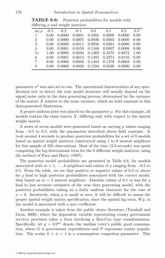
176 Introduction to Spatial Econometrics
TABLE 6.6: Posterior probabilities for models withdiffering ρ and weight matrices
m/ρ -0.5 -0.2 -0.1 0.0 0.1 0.2 0.51 0.00 0.0000 0.0001 0.1091 0.0000 0.0000 0.002 0.00 0.0000 0.0007 0.0936 0.0003 0.0000 0.003 0.00 0.0000 0.0011 0.0956 0.0364 0.0000 0.004 0.00 0.0001 0.0559 0.1168 0.0907 0.0008 0.005∗ 1.00 0.9998 0.8694 0.1369 0.4273 0.9872 1.006 0.00 0.0001 0.0612 0.1402 0.2374 0.0116 0.007 0.00 0.0000 0.0086 0.1484 0.1479 0.0003 0.008 0.00 0.0000 0.0029 0.1594 0.0599 0.0000 0.00
parameter σ2 was also set to one. The operational characteristics of any spec-ification test to detect the true model structure will usually depend on thesignal/noise ratio in the data generating process, determined by the varianceof the matrix X relative to the noise variance, which we hold constant in thisdata-generated illustration.
A proper uniform prior was placed on the parameter ρ. For this example, allmodels contain the same matrix X , differing only with respect to the spatialweight matrix.
A series of seven models were generated based on varying ρ values rangingfrom −0.5 to 0.5, with the parameters described above held constant. Ittook around 4 seconds to produce posterior probabilities for a set of 8 modelsbased on spatial weight matrices constructed using 1 to 8 nearest neighborsfor this sample of 258 observations. Most of the time (3.3 seconds) was spentcomputing the log-determinant term for the 8 different weight matrices, usingthe method of Pace and Barry (1997).
The posterior model probabilities are presented in Table 6.6, for modelsassociated with m = 1, . . . , 8 neighbors and values of ρ ranging from −0.5 to0.5. From the table, we see that positive or negative values of 0.2 or abovefor ρ lead to high posterior probabilities associated with the correct model,that based on m = 5 nearest neighbors. Absolute values of 0.1 or less for ρlead to less accurate estimates of the true data generating model, with theposterior probabilities taking on a fairly uniform character for the case ofρ = 0. Intuitively, when ρ is small or zero, it will be difficult to assess theproper spatial weight matrix specification, since the spatial lag term, Wy, inthe model is associated with a zero coefficient.
Another example is taken from the public choice literature (Turnbull andGeon, 2006), where the dependent variable representing county governmentservices provision takes a form involving a Box-Cox type transformation.Specifically, let g = GPφ denote the median voter’s public good consump-tion, where G is government expenditures and P represents county popula-tion. The scalar 0 < φ < 1 is a consumption congestion parameter. This
© 2009 by Taylor & Francis Group, LLC
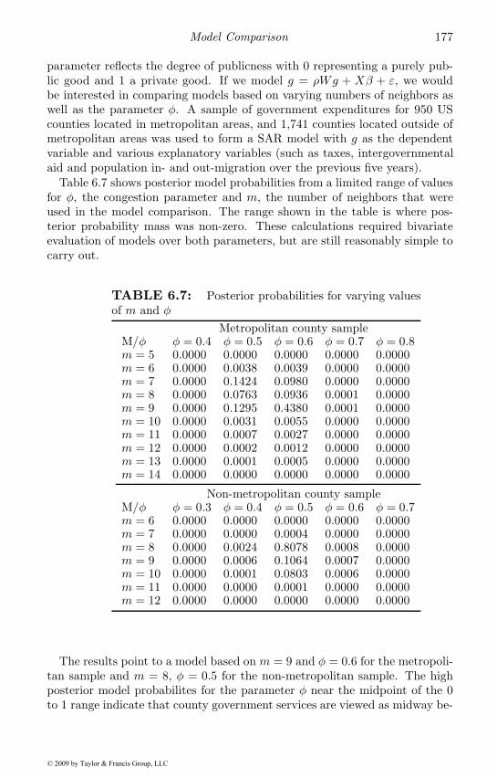
Model Comparison 177
parameter reflects the degree of publicness with 0 representing a purely pub-lic good and 1 a private good. If we model g = ρWg + Xβ + ε, we wouldbe interested in comparing models based on varying numbers of neighbors aswell as the parameter φ. A sample of government expenditures for 950 UScounties located in metropolitan areas, and 1,741 counties located outside ofmetropolitan areas was used to form a SAR model with g as the dependentvariable and various explanatory variables (such as taxes, intergovernmentalaid and population in- and out-migration over the previous five years).
Table 6.7 shows posterior model probabilities from a limited range of valuesfor φ, the congestion parameter and m, the number of neighbors that wereused in the model comparison. The range shown in the table is where pos-terior probability mass was non-zero. These calculations required bivariateevaluation of models over both parameters, but are still reasonably simple tocarry out.
TABLE 6.7: Posterior probabilities for varying valuesof m and φ
Metropolitan county sampleM/φ φ = 0.4 φ = 0.5 φ = 0.6 φ = 0.7 φ = 0.8m = 5 0.0000 0.0000 0.0000 0.0000 0.0000m = 6 0.0000 0.0038 0.0039 0.0000 0.0000m = 7 0.0000 0.1424 0.0980 0.0000 0.0000m = 8 0.0000 0.0763 0.0936 0.0001 0.0000m = 9 0.0000 0.1295 0.4380 0.0001 0.0000m = 10 0.0000 0.0031 0.0055 0.0000 0.0000m = 11 0.0000 0.0007 0.0027 0.0000 0.0000m = 12 0.0000 0.0002 0.0012 0.0000 0.0000m = 13 0.0000 0.0001 0.0005 0.0000 0.0000m = 14 0.0000 0.0000 0.0000 0.0000 0.0000
Non-metropolitan county sampleM/φ φ = 0.3 φ = 0.4 φ = 0.5 φ = 0.6 φ = 0.7m = 6 0.0000 0.0000 0.0000 0.0000 0.0000m = 7 0.0000 0.0000 0.0004 0.0000 0.0000m = 8 0.0000 0.0024 0.8078 0.0008 0.0000m = 9 0.0000 0.0006 0.1064 0.0007 0.0000m = 10 0.0000 0.0001 0.0803 0.0006 0.0000m = 11 0.0000 0.0000 0.0001 0.0000 0.0000m = 12 0.0000 0.0000 0.0000 0.0000 0.0000
The results point to a model based on m = 9 and φ = 0.6 for the metropoli-tan sample and m = 8, φ = 0.5 for the non-metropolitan sample. The highposterior model probabilites for the parameter φ near the midpoint of the 0to 1 range indicate that county government services are viewed as midway be-
© 2009 by Taylor & Francis Group, LLC
178 Introduction to Spatial Econometrics
tween the extremes of pure public and private goods. For the US counties, theaverage number of first-order contiguous neighbors (those with borders thattouch each county) is around 6, so the number of neighbors chosen from themodel comparison exercise represents slightly more than just the contiguouscounties.
6.3.4 An illustration of MC3 and model averaging
We use a 49 neighborhood data set for Columbus, Ohio from Anselin(1988) that contains observations on the median housing values (hvalue) foreach neighborhood and household income (income) as explanatory variables.Neighborhood crime is the dependent variable in the model that we use toillustrate MC3 and model averaging.
As already noted, if the data generating process is the SAR model, thenβSAR = (X ′X)−1X ′(In − ρW )y, and least-squares estimates for β are biasedand inconsistent. In these cases, we would expect that regression-based MC3
procedures would not produce accurate estimates and inferences regardingwhich variables are important.
To illustrate differences between non-spatial and spatial MC3 and modelaveraging results, we estimate an SDM model as well as the SLX model usingstandard methods. The SDM model is shown in (6.24). Intuitively, housingvalues and household income levels in nearby neighborhoods might contributeto explaining variation in neighborhood crime rates, y.
y = αιn + ρWy + β1hvalue+ β2income+ β3W · hvalue+ β4W · income+ ε (6.24)
y = ρWy +Xβ +WXθ + ε
The contiguity-based weight matrix from Anselin (1988) was used to pro-duce standard estimates in Table 6.8. The greatest disagreement in the twosets of estimates is with respect to the two spatially lagged explanatory vari-ables, which could be a focus of model comparison and inference. For example,it might be of interest whether housing values and household income levelsin nearby neighborhoods contribute to explaining variation in neighborhoodcrime rates. For later reference, we note that the sign of the spatially laggedhouse value variable is different in the SLX (least-squares) and SDM regres-sions, and the significance of the spatial lag of household income is different.
For ourMC3 procedure, the intercept term and spatial lag of the dependentvariable are included in all models. This leads to four candidate variables and24 = 16 possible models. This makes it simple to validate ourMC3 algorithmsby comparison with exact results based on posterior model probabilities forthe set of 16 models. The explanatory variables were put in deviation from themeans form and scaled by their standard deviations, and the Zellner g-priorwas used in the MC3 procedure.
© 2009 by Taylor & Francis Group, LLC
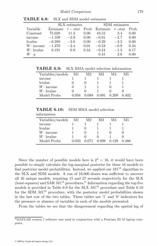
Model Comparison 179
TABLE 6.8: SLX and SDM model estimatesSLX estimates SDM estimates
Variable Estimate t− stat Prob Estimate t−stat ProbConstant 75.028 11.3 0.00 43.52 3.4 0.00income −1.109 −2.9 0.00 −0.91 −2.7 0.00hvalue −0.289 −2.8 0.00 −0.29 −3.2 0.00W · income −1.370 −2.4 0.01 −0.53 −0.9 0.34W · hvalue 0.191 0.9 0.34 −0.24 −1.3 0.17W · y 0.41 2.6 0.00
TABLE 6.9: SLX BMA model selection informationVariables/models M1 M2 M3 M4 M5income 1 1 1 1 1hvalue 0 0 1 1 1W · income 0 1 1 0 1W · hvalue 0 0 1 0 0Model Probs 0.056 0.088 0.091 0.209 0.402
TABLE 6.10: SDM BMA model selectioninformation
Variables/models M1 M2 M3 M4 M5income 1 1 1 1 1hvalue 1 0 1 1 1W · income 1 0 1 0 0W · hvalue 1 0 0 1 0Model Probs 0.033 0.071 0.098 0.128 0.486
Since the number of possible models here is 24 = 16, it would have beenpossible to simply calculate the log-marginal posterior for these 16 models tofind posterior model probabilities. Instead, we applied our MC3 algorithm tothe SLX and SDM models. A run of 10,000 draws was sufficient to uncoverall 16 unique models, requiring 15 and 27 seconds respectively for the SLX(least-squares) and SARMC3 procedures.6 Information regarding the top fivemodels is provided in Table 6.9 for the SLX MC3 procedure and Table 6.10for the SDM MC3 procedure, with the posterior model probabilities shownin the last row of the two tables. These tables use ‘1’ and ‘0’ indicators forthe presence or absence of variables in each of the models presented.
From the tables we see that the disagreement regarding the spatial lag of
6MATLAB version 7 software was used in conjunction with a Pentium III M laptop com-puter.
© 2009 by Taylor & Francis Group, LLC
180 Introduction to Spatial Econometrics
household income between the two models appears in the MC3 results asit did in the basic model estimates. The model with the highest posteriormodel probability from the SLX MC3 procedure includes household incomefrom neighboring regions, whereas this variable appears in a model having thethird highest posterior probability in the SDM results.
It is instructive to see how Bayesian model averaging can help to resolvethe issue regarding the significance of the spatial lag of household income.Model averaged estimates based on a posterior model probability weightedcombination of MCMC draws from estimation of all 16 models are shown inTable 6.11. The results from the SLX model averaging procedure were con-structed using Bayesian MCMC sampling for the SLX model with a diffuseprior. A similar MCMC procedure with a diffuse prior was used to constructdraws for the SDM model. Having draws from MCMC is convenient becausethese can be weighted by the posterior model probabilities to form a posteriordistribution that reflects the model uncertainty that model averaging proce-dures attempt to capture. The table reports means as well as 0.95 credibleintervals constructed using the simulation draws.
The SLX model resolved the question of importance for the spatial lag ofincome in favor of this variable being included in the model, whereas the spa-tial lag of neighboring house values (hvalue) does not appear important in thismodel. It is interesting to note that the averaged coefficients for both incomeand W · income are smaller in value than those from standard least-squaresestimation. This reduction in magnitude arises from taking into account ouruncertainty regarding the appropriate model specification. The reduction incoefficient magnitude due to model uncertainty also makes it clearer that thespatial lag of hvalue is not an important variable when one takes into accountalternative model specifications. However, we will have more to say aboutthis later.
We see a similar reduction in magnitude for the averaged coefficients versusthose from standard estimation of the SDM model that ignores model uncer-tainty. The reduction in magnitudes here points to a lack of importance forthe spatial lags of income and hvalue. However, we need to calculate directand indirect effects estimates to draw conclusions about the magnitude ofimpact on neighborhood crime associated with changes in these variables. Infact, in the SLX model we have direct and indirect effects that result in atotal effect as well. This can be seen by considering the partial derivative of yfor this model with respect to the explanatory variables X . This would takea form involving both the coefficients on income and hvalue as well as thespatial lags of these variables. Specifically, the matrix Sr(W ) = Inβr +Wθrarises from the partial derivative calculation. In a way, these effects do notrequire calculation, since the mean direct effects are the coefficients on thenon-spatial variables and the mean indirect effects are those associated withthe spatial lags of the explanatory variables. The mean total effects are simplythe sum of these two coefficients. However, if we wish to construct confidenceintervals on these impacts we can use the MCMC draws to do this.
© 2009 by Taylor & Francis Group, LLC
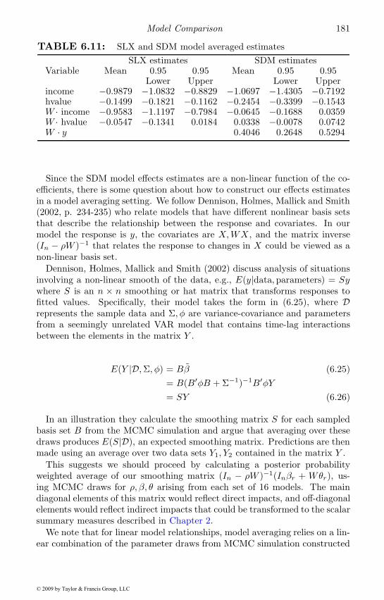
Model Comparison 181
TABLE 6.11: SLX and SDM model averaged estimatesSLX estimates SDM estimates
Variable Mean 0.95 0.95 Mean 0.95 0.95Lower Upper Lower Upper
income −0.9879 −1.0832 −0.8829 −1.0697 −1.4305 −0.7192hvalue −0.1499 −0.1821 −0.1162 −0.2454 −0.3399 −0.1543W · income −0.9583 −1.1197 −0.7984 −0.0645 −0.1688 0.0359W · hvalue −0.0547 −0.1341 0.0184 0.0338 −0.0078 0.0742W · y 0.4046 0.2648 0.5294
Since the SDM model effects estimates are a non-linear function of the co-efficients, there is some question about how to construct our effects estimatesin a model averaging setting. We follow Dennison, Holmes, Mallick and Smith(2002, p. 234-235) who relate models that have different nonlinear basis setsthat describe the relationship between the response and covariates. In ourmodel the response is y, the covariates are X,WX , and the matrix inverse(In − ρW )−1 that relates the response to changes in X could be viewed as anon-linear basis set.
Dennison, Holmes, Mallick and Smith (2002) discuss analysis of situationsinvolving a non-linear smooth of the data, e.g., E(y|data, parameters) = Sywhere S is an n × n smoothing or hat matrix that transforms responses tofitted values. Specifically, their model takes the form in (6.25), where Drepresents the sample data and Σ, φ are variance-covariance and parametersfrom a seemingly unrelated VAR model that contains time-lag interactionsbetween the elements in the matrix Y .
E(Y |D,Σ, φ) = Bβ (6.25)= B(B′φB + Σ−1)−1B′φY= SY (6.26)
In an illustration they calculate the smoothing matrix S for each sampledbasis set B from the MCMC simulation and argue that averaging over thesedraws produces E(S|D), an expected smoothing matrix. Predictions are thenmade using an average over two data sets Y1, Y2 contained in the matrix Y .
This suggests we should proceed by calculating a posterior probabilityweighted average of our smoothing matrix (In − ρW )−1(Inβr + Wθr), us-ing MCMC draws for ρ, β, θ arising from each set of 16 models. The maindiagonal elements of this matrix would reflect direct impacts, and off-diagonalelements would reflect indirect impacts that could be transformed to the scalarsummary measures described in Chapter 2.
We note that for linear model relationships, model averaging relies on a lin-ear combination of the parameter draws from MCMC simulation constructed
© 2009 by Taylor & Francis Group, LLC
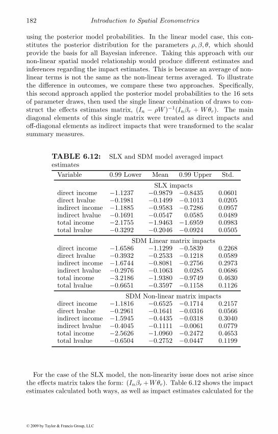
182 Introduction to Spatial Econometrics
using the posterior model probabilities. In the linear model case, this con-stitutes the posterior distribution for the parameters ρ, β, θ, which shouldprovide the basis for all Bayesian inference. Taking this approach with ournon-linear spatial model relationship would produce different estimates andinferences regarding the impact estimates. This is because an average of non-linear terms is not the same as the non-linear terms averaged. To illustratethe difference in outcomes, we compare these two approaches. Specifically,this second approach applied the posterior model probabilities to the 16 setsof parameter draws, then used the single linear combination of draws to con-struct the effects estimates matrix, (In − ρW )−1(Inβr + Wθr). The maindiagonal elements of this single matrix were treated as direct impacts andoff-diagonal elements as indirect impacts that were transformed to the scalarsummary measures.
TABLE 6.12: SLX and SDM model averaged impactestimates
Variable 0.99 Lower Mean 0.99 Upper Std.
SLX impactsdirect income −1.1237 −0.9879 −0.8435 0.0601direct hvalue −0.1981 −0.1499 −0.1013 0.0205indirect income −1.1885 −0.9583 −0.7286 0.0957indirect hvalue −0.1691 −0.0547 0.0585 0.0489total income −2.1755 −1.9463 −1.6959 0.0983total hvalue −0.3292 −0.2046 −0.0924 0.0505
SDM Linear matrix impactsdirect income −1.6586 −1.1299 −0.5839 0.2268direct hvalue −0.3932 −0.2533 −0.1218 0.0589indirect income −1.6744 −0.8081 −0.2756 0.2973indirect hvalue −0.2976 −0.1063 0.0285 0.0686total income −3.2186 −1.9380 −0.9749 0.4630total hvalue −0.6651 −0.3597 −0.1158 0.1126
SDM Non-linear matrix impactsdirect income −1.1816 −0.6525 −0.1714 0.2157direct hvalue −0.2961 −0.1641 −0.0316 0.0566indirect income −1.5945 −0.4435 −0.0318 0.3040indirect hvalue −0.4045 −0.1111 −0.0061 0.0779total income −2.5626 −1.0960 −0.2472 0.4653total hvalue −0.6504 −0.2752 −0.0447 0.1199
For the case of the SLX model, the non-linearity issue does not arise sincethe effects matrix takes the form: (Inβr+Wθr). Table 6.12 shows the impactestimates calculated both ways, as well as impact estimates calculated for the
© 2009 by Taylor & Francis Group, LLC
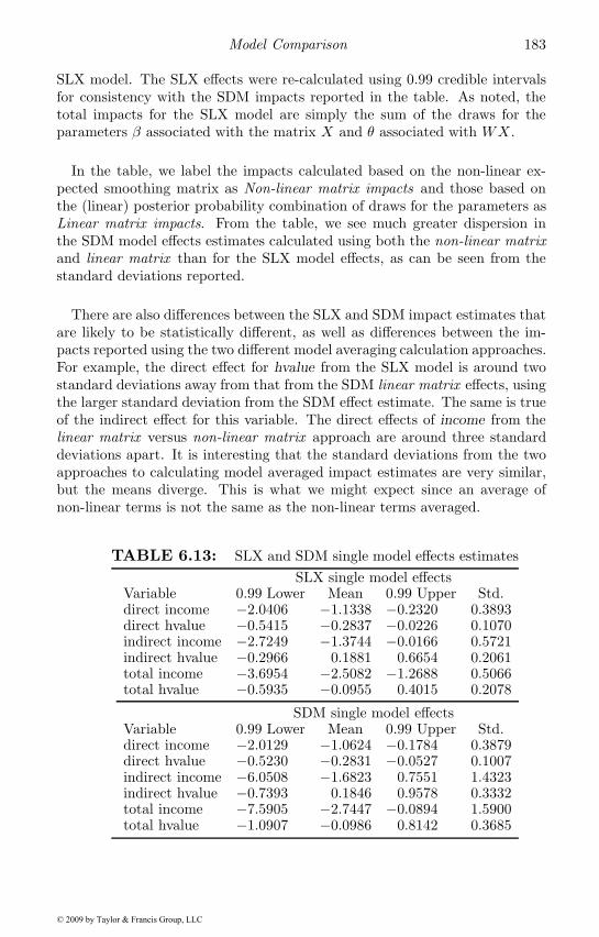
Model Comparison 183
SLX model. The SLX effects were re-calculated using 0.99 credible intervalsfor consistency with the SDM impacts reported in the table. As noted, thetotal impacts for the SLX model are simply the sum of the draws for theparameters β associated with the matrix X and θ associated with WX .
In the table, we label the impacts calculated based on the non-linear ex-pected smoothing matrix as Non-linear matrix impacts and those based onthe (linear) posterior probability combination of draws for the parameters asLinear matrix impacts. From the table, we see much greater dispersion inthe SDM model effects estimates calculated using both the non-linear matrixand linear matrix than for the SLX model effects, as can be seen from thestandard deviations reported.
There are also differences between the SLX and SDM impact estimates thatare likely to be statistically different, as well as differences between the im-pacts reported using the two different model averaging calculation approaches.For example, the direct effect for hvalue from the SLX model is around twostandard deviations away from that from the SDM linear matrix effects, usingthe larger standard deviation from the SDM effect estimate. The same is trueof the indirect effect for this variable. The direct effects of income from thelinear matrix versus non-linear matrix approach are around three standarddeviations apart. It is interesting that the standard deviations from the twoapproaches to calculating model averaged impact estimates are very similar,but the means diverge. This is what we might expect since an average ofnon-linear terms is not the same as the non-linear terms averaged.
TABLE 6.13: SLX and SDM single model effects estimatesSLX single model effects
Variable 0.99 Lower Mean 0.99 Upper Std.direct income −2.0406 −1.1338 −0.2320 0.3893direct hvalue −0.5415 −0.2837 −0.0226 0.1070indirect income −2.7249 −1.3744 −0.0166 0.5721indirect hvalue −0.2966 0.1881 0.6654 0.2061total income −3.6954 −2.5082 −1.2688 0.5066total hvalue −0.5935 −0.0955 0.4015 0.2078
SDM single model effectsVariable 0.99 Lower Mean 0.99 Upper Std.direct income −2.0129 −1.0624 −0.1784 0.3879direct hvalue −0.5230 −0.2831 −0.0527 0.1007indirect income −6.0508 −1.6823 0.7551 1.4323indirect hvalue −0.7393 0.1846 0.9578 0.3332total income −7.5905 −2.7447 −0.0894 1.5900total hvalue −1.0907 −0.0986 0.8142 0.3685
© 2009 by Taylor & Francis Group, LLC
184 Introduction to Spatial Econometrics
Finally, it is of interest to compare the impact estimates from a single modelversus those based on the model averaging procedure. These are shown in Ta-ble 6.13, for a saturated version of both the SLX and SDM models, where allvariables were included during estimation. Focusing on the SLX effects es-timates, we see the same pattern of shrinkage towards zero for the modelaveraged estimates relative to those from the saturated model, reflecting therole of model uncertainty. We also see that the saturated model producedmuch larger standard deviations, or dispersion in the effects estimates, pre-sumably due to the inclusion of all variables in the saturated model. Thisreflects the classic trade-off between attempting to include a sufficient num-ber of variables to overcome potential omitted variables bias and inclusion ofredundant variables that decrease precision of the estimates. It is preciselythis trade-off that model averaging seeks to address. A comparison of the twosets of SLX effects estimates suggests that model averaging was successful inthis regard. It is also of interest that the model averaged effects lead us toinfer that the total impacts from both variables are negative and significant.In contrast, the single saturated model estimates suggest that the total effectof hvalue is not significant.
We compare the non-linear matrix model averaged SDM impact estimatesto those from the single saturated model in Table 6.13. Again, the meanimpact estimates are relatively smaller for the model averaged estimates thanthe saturated single model. Again, this suggests that model averaging iscapturing our uncertainty about the model specification. With regard tothe dispersion of the single model estimates and that of the model averagedestimates we also see the same pattern as with the SLX effects estimates.The model averaged estimates exhibit less dispersion, which can be seen bycomparing the standard deviations reported in both tables. This implies thatthe saturated model is suffering from the classic over-inclusion of redundantvariables, and model averaged effects estimates improve on this situation.As in the case of the single model SLX effects estimates, the SDM modeleffects from the single saturated model would lead to the conclusion that thetotal effect of hvalue is not significant, whereas both sets of model averagedestimates show a negative and significant total effect for this variable.
6.4 Chapter summary
A number of issues arise in applied modeling regarding model specification.In the case of spatial regression models these include questions regarding thetype of spatial weight matrix to use as well as the usual uncertainty aboutexplanatory variables.
A desirable extension of the MC3 methodology and model averaging would
© 2009 by Taylor & Francis Group, LLC
Model Comparison 185
be to determine both the spatial weight matrix and explanatory variables. Wenote that explanatory variables determined using the MC3 methodology pre-sented here were conditional on the specific spatial weight matrix employed.LeSage and Fischer (2008) extend the MC3 approach of LeSage and Parent(2007) presented here to accomplish this. The extension introduces a “birthstep” and “death step” that can be used to increase or decrease the numberof nearest neighbors in the spatial weight matrix.
There are other approaches to Bayesian model comparison that representapproximations to the log-marginal likelihood needed to calculate posteriormodel probabilities. These methods are useful where it is difficult or impos-sible to carry out integration of the parameters that arise in the log-marginallikelihood expression. For example, Parent and LeSage (2008) use a methodproposed by Chib (1995), and Chib and Jeliazkov (2001) to compare a hostof alternative non-nested spatial model specifications based on varying typesof spatial, technological and transport connectivity of European regions. Thismethod approximates the log-marginal likelihood using MCMC draws of theparameters to “integrate” these out of the expression for the log-marginallikelihood.
A simple procedure proposed by Newton and Raftery (1994) is to evaluatethe log-likelihood function on each pass through the MCMC sampler andcalculate a harmonic mean of these values as an approximation to the log-marginal likelihood. This approach is illustrated in LeSage and Polasek (2008)to compare models of the type discussed in Chapter 8 based on two differentspatial weight matrices.
6.5 Chapter appendix
In this appendix, we describe a computationally efficient approach to eval-uating four separate terms involved in the univariate integration problem overthe range of support for the parameter ρ in the SAR model. In the context ofthe MC3 described in Section 6.3 there is a need for a computationally fastscheme for the univariate integration. This must be carried out on every passthrough the MCMC sampler which occurs thousands of times.
The four terms in (6.18) for the SAR model that vary with ρ are shown in(6.27) as T1, T2, T3 and T4.
© 2009 by Taylor & Francis Group, LLC
186 Introduction to Spatial Econometrics
T1(ρ) = |In − ρW | (6.27)
T2(ρ) = [(In − ρW )y −Xβ(ρ) − αιn]′[(In − ρW )y −Xβ(ρ) − αιn]
T3(ρ) = (g
1 + g)β(ρ)′X ′Xβ(ρ)
T4(ρ) =1
Beta(d, d)(1 + ρ)d−1(1 − ρ)d−1
22d−1
A log transformation can be applied to all terms T1, . . . , T4, allowing us torely on computationally fast methods presented in Pace and Barry (1997) andBarry and Pace (1999) to compute the log-determinant in T1 (see Chapter 4).
Pace and Barry (1997) also suggest a vectorization of the terms in T1 andT2 that we used in Chapter 3 for maximum likelihood estimation of the SARmodel. This involves constructing log-determinant values over a grid of qvalues of ρ, which is central to our task of integration for the terms T1(ρ)and T2(ρ). In applied work involving the SAR model, we typically rely on arestriction of ρ to the (−1, 1) or [0, 1) interval to avoid the need to computeeigenvalues.
Turning attention to the term T2(ρ), we follow Chapter 3 and write theterm, [(In − ρW )y−Xβ(ρ)− αιn]′[(In − ρW )y−Xβ(ρ)− αιn] as a vector inq values of ρ. For our problem we have the expression shown in (6.28).
T2(ρi) = e(ρi)′e(ρi), i = 1, . . . , q (6.28)
With:
e(ρi) = eo − ρied
eo = y −Xβo − αoιn
ed = Wy −Xβd − αdιn
βo = (X ′X)−1X ′yβd = (X ′X)−1X ′Wy
αo = y
αd = Wy (6.29)
The term T3 can be vectorized using a loop over ρi values along with theexpression β(ρ) = βo − ρiβd. Finally, the term T4(ρ) representing the prioron the parameter ρ is simple to compute over a grid of q values for ρ, andtransform to logs.
One important point to note is that we do not need to estimate the modelparameters η = (α, β, σ, ρ) to carry out numerical integration leading to pos-terior model probabilities. Intuitively, we have analytically integrated theparameters α, β and σ out of the problem, leaving only a univariate integralin ρ. Given any sample data y,X along with a spatial weight matrix W , we
© 2009 by Taylor & Francis Group, LLC
Model Comparison 187
can rely on the Pace and Barry (1997) vectorization scheme applied to ourtask. This involves evaluating the log-marginal density terms T1, . . . , T4 overa fine grid of q values for ρ ranging over the interval (−1, 1). Given a matrixof vectorized log-marginal posteriors, integration can be accomplished usingSimpson’s rule.
Further computational savings can be achieved by noting that the gridcan be rough, say based on 0.01 increments in ρ, which speeds the directsparse matrix approach of Pace and Barry (1997) or Barry and Pace (1999)computations. Spline interpolation can then be used to produce a much finergrid very quickly, as the log-determinant is typically quite well-behaved forreasonably large spatial samples in excess of 250 observations.
Another important point concerns scaling which is necessary to carry outnumerical integration for the anti-log of the log-marginal posterior density.Our approach allows one to evaluate log-marginal posteriors for each modelunder consideration and store these as vectors ranging over the grid of ρvalues. Scaling then involves finding the maximum of these vectors placed ascolumns in a matrix, (e.g. the maximum from all columns in the matrix).This maximum is then subtracted from all elements in the matrix of log-marginals, producing a value of zero as the largest element, so the anti-log isunity. This approach to scaling provides an elegant solution that requires nouser-intervention and works for all problems.
© 2009 by Taylor & Francis Group, LLC

Chapter 7
Spatiotemporal and Spatial Models
Unlike the previous chapters, this chapter is more theoretical and concentrateson the spatiotemporal foundations of spatial models. To achieve this goal, weassume that regions are only influenced by their own and other regions’ pastvariables (no simultaneous influence). We show that this strict spatiotemporalframework results in a long-run equilibrium characterized by simultaneousspatial dependence. Note, we specifically avoid assuming spatial simultaneityin the spatiotemporal process as this would be assuming what we are tryingto show. To keep the exposition as simple as possible and to expose relationsamong some of the common models we employ a number of assumptions suchas symmetric W , constant or deterministically growing X , and no structuralchange over time.
Strictly temporal models provide our starting point, and econometrics pro-vides a rich set of non-spatial temporal models grounded in economic theory.Partial adjustment models provide a classic example of this type of model.Partial adjustment models as well as other motivations give rise to specifi-cations that employ temporal lags of both the dependent and explanatoryvariables.
In the context of regional data, conventional temporal models allow thedependent variable yt for each region to be temporally dependent on pastperiod values yt−j , j = 1, . . . , j − 1 of the own region. These conventionaltemporal models can be reasonably modified to allow for spatial dependenceon other regions through time using spatial lags of the time lags (space-timelags) Wyt−1 and WXt−1. These can be incorporated into the model in ad-dition to conventional temporal lags, yt−1 and Xt−1, leading to a form ofspatiotemporal model.
We have already noted that cross-sectional spatial lag models such as theSAR exhibit simultaneous dependence which may seem counterintuitive insome applied settings. However, cross-sectional spatial dependence can arisefrom a diffusion process working over time rather than occurring simultane-ously. In this chapter we explore how spatiotemporal processes working overtime can lead to equilibrium outcomes that exhibit spatial dependence. Ourfocus is on the spatiotemporal underpinnings of the cross-sectional spatialdependence that we often observe in regional data samples. We show howspatiotemporal data generating processes are related to many of the cross-sectional models popular in spatial econometrics and statistics. In addition,
189© 2009 by Taylor & Francis Group, LLC
190 Introduction to Spatial Econometrics
this analysis suggests more complicated spatial models for further exploration.
7.1 Spatiotemporal partial adjustment model
We provide a simple generalization of the well-known partial adjustmentmodel to illustrate how temporal models can be adapted to a spatiotemporalsetting. The temporal partial adjustment development in Greene (1997, p.698-799) serves as a starting point, but we extend this to a spatiotemporalsetting. The basic equations for our spatial partial adjustment model are in(7.1)–(7.3).
y∗t = Utψ +WUtγ + αιn (7.1)yt = (1 − φ)y∗t + φG1yt−1 + εt (7.2)G1 = θIn + πW (7.3)
Let y∗t denote the equilibrium value of the dependent variable, yt. Then× p matrix Ut contains non-constant exogenous explanatory variables, andthe n×1 vector of disturbances εt are distributed N(0, σ2In). The parameterφ governs the degree of partial adjustment between previous values of thedependent variable, yt−1 and the equilibrium values y∗t . The parameters ψcapture the effect of own-region explanatory variables, γ captures the effectsof explanatory variables at nearby locations, and α is an intercept parame-ter. The scalar parameters θ, π measure the extent of temporal and spatialdependence captured by the n× n matrix G1.
The equilibrium level of the dependent variable, y∗t , depends upon the ex-planatory variables of the own observations (Ut), nearby observations reflectedin the spatial lag (WUt), and an intercept (ιn). The parameters associatedwith these explanatory variables are ψ, γ, and α. This type of model spec-ifies observed yt as a linear combination (governed by φ) of the equilibriumlevels y∗t and past values of the dependent variable (yt−1) as well as nearbydependent variables reflected by the spatiotemporal lag vector (Wyt−1).
Manipulating (7.1)–(7.3) yields (7.4) indicating that yt depends on: tem-poral and space-time lags of the dependent variable (Gyt−1), spatial lags ofthe explanatory variables (WUt), in addition to the conventional relationshipinvolving the explanatory variables Ut.
yt = Ut(1 − φ)ψ +WUt(1 − φ)γ + ιn(1 − φ)α + φG1yt−1 + εt (7.4)
As a concrete example, consider the situation faced by retailers. The salesperformance of retail stores is often modeled as a function of the store’s size
© 2009 by Taylor & Francis Group, LLC
Spatiotemporal and Spatial Models 191
and the sizes of competitor stores. For retail activities involving commodi-ties such as groceries, hardware, and clothing, stores that are located nearbyrepresent the competition.
For this retailing example, suppose the variable Ut represents store size andthe spatial lag variable WUt the average size of nearby stores (competitors).If yt measures store sales, these should be positively related to own store sizeand inversely to competitor store sizes. The desired level y∗t is the expectedstore sales given the size of the store and that of competitor stores. Previousstore sales and previous sales of competitors also influence current store sales.Lee and Pace (2005) fitted a spatiotemporal model (with simultaneous spatialcomponents) to store sales in Houston and found strong spatial dependence.Store size was found to be important and store sales exhibited strong temporalas well as spatial dependence.
We can simplify (7.4) using the symbols defined in (7.6) to represent theunderlying structural parameter combinations and combining the explanatoryvariables into a single matrix Xt. This results in a classic spatiotemporalmodel in (7.5).
yt = Xtβ +Gyt−1 + εt (7.5)
G = τIn + ρW, τ = φθ, ρ = φπ, β = (1 − φ)[ψ γ α
]′ (7.6)
Xt =[Ut WUt ιn
]To summarize, a minor change in some of the models used to motivate tem-
poral lags of the explanatory and dependent variables in non-spatial econo-metrics can lead to a spatiotemporal specification such as (7.5). Section 7.2discusses the relation between spatiotemporal models and cross-sectional spa-tial models.
7.2 Relation between spatiotemporal and SAR models
As briefly discussed in Chapter 1, we can relate cross-sectional spatial mod-els to long-run equilibria associated with spatiotemporal models. In this sec-tion, we generalize the simple motivational example from Chapter 1 to ex-plore the relation between spatiotemporal and spatial models. We will usethe relationship derived here to show how a spatiotemporal mechanism (per-haps arising from the partial adjustment mechanism discussed in the previoussection) can yield many of the cross-sectional models discussed in the spatialstatistics and spatial econometrics literature. We note that the partial adjust-ment motivation from the previous section is not the only way to motivate aspatiotemporal generating process. Our developments apply more generally
© 2009 by Taylor & Francis Group, LLC
192 Introduction to Spatial Econometrics
to the relation between spatiotemporal processes and cross-sectional spatialmodels, and we use these relationships to motivate new spatial specifications.
We begin with the model in (7.7), where yt is an n× 1 dependent variablevector at time t (t ≥ 0), and the n × k matrix Xt represents explanatoryvariables. As illustrated in the previous section, Xt could contain spatial lagsof the explanatory variables. This is a generalization of the spatial temporalautoregressive model (STAR) (Pfeifer and Deutsch, 1980; Cressie, 1993; Paceet al., 2000) that relies on past period dependent variables and contains nosimultaneous spatial interaction. We will show that this dynamic relationshipimplies a cross-sectional steady state that can be viewed as a simultaneousspatial interaction.
Note, we specifically avoid assuming any form of simultaneous spatial de-pendence in the spatiotemporal process itself as this would be assuming whatwe are trying to demonstrate (how simultaneous spatial dependence arises).
yt = Gyt−1 +Xtβ + vt (7.7)Xt = ϕtX0 (7.8)G = τIn + ρW (7.9)dt = Xtγ (7.10)vt = r + dt + εt (7.11)
The scalar parameter τ governs dependence between each region at time t andt − 1, while the scalar parameter ρ reflects spatial dependence between eachregion at time t and neighboring regions at time t−1. The scalar parameter ϕallows the explanatory variables to grow at a constant rate (ϕ) per period (asopposed to holding explanatory variables constant over time as in Chapter 1).A value of ϕ = 1 represents no growth in X0 over time and values ϕ > 1 allowfor growth in the explanatory variables. We assume ϕ > τ .
As before, the spatial weight matrix W is an n×n exogenous non-negativematrix. We assumeW is symmetric and scaled to have a maximum eigenvalueof 1 with a minimum eigenvalue that is greater than or equal to −1. Scalingany symmetric weight matrix by its maximum eigenvalue provides one way ofobtaining a symmetric W with a maximum eigenvalue of 1. Alternatively, asymmetric doubly stochastic W has a maximum eigenvalue of 1.
Given that G is composed of the identity matrix and a symmetric weightmatrix W , it is symmetric as well. Since G is real and symmetric, it has n realeigenvalues and a full rank set of n orthogonal real eigenvectors. The largestmagnitude eigenvalue of G equals τ + ρ. We assume the following stabilityrestrictions in (7.12)
(τ + ρ)t < κ, ρ ∈ [0, 1), τ ∈ [0, 1) (7.12)
where κ is a small positive constant. This will ensure that for sufficientlylarge values of t, we can assume that Gt takes on the small values required
© 2009 by Taylor & Francis Group, LLC
Spatiotemporal and Spatial Models 193
for our analysis. Although we could examine negative τ and ρ, we choose tolook only at positive ρ and τ to simplify the exposition and because negativeρ and τ are of minor interest.
In Chapter 2 we considered the role of omitted variables which we general-ize here. The generalization involves assuming the overall n × 1 disturbancevector vt can be partitioned into three components. These components repre-sent omitted variables independent of the explanatory variables (r), omittedvariables correlated with the explanatory variables (dt), and a random noiseterm (εt). The first component is an n×1 vector r that captures omitted vari-ables uncorrelated with Xt that remain constant over time. These might beamenities, region specific attributes such as land or water area, border lengthsof the regions or difficult-to-specify locational discounts and premia. For sim-plicity, we assume that r is distributed N(0, σ2
rIn). The second componentis an n × 1 vector dt = Xtγ representing the effect of omitted variables thatare correlated with Xt, where γ �= 0 reflects the strength of correlation. Thiscomponent can grow or decrease over time since Xt = ϕtX0. The third com-ponent is a random n× 1 vector εt that we assume is distributed N(0, σ2
εIn)and independent of εt−i for i ∈ (0, t]. We further assume that εt−i for i ∈ [0, t]is independent of r and Xt.
The STAR model uses only past dependent variables and current inde-pendent variables to explain variation in the current dependent variable vec-tor. Following Elhorst (2001) we use the recursive relation: yt−1 = Gyt−2 +Xt−1β + r + dt−1 + εt−1 implied by the model in (7.7) to consider the stateof this dynamic system after passage of t time periods, which is shown in(7.13)–(7.17).
yt = (Inϕt +Gϕt−1+, . . . ,+Gt−1ϕ)X0β +Gty0 + z (7.13)z = z1 + z2 + z3 (7.14)z1 = (In +G+, . . . ,+Gt−1)r (7.15)z2 = (Inϕt +Gϕt−1+, . . . ,+Gt−1ϕ)X0γ (7.16)z3 = εt +Gεt−1 +G2εt−2+, . . . ,+Gt−1ε1 (7.17)
Taking the expectation of the dependent variable in (7.13) for sufficientlylarge t yields the long-run equilibrium as shown in (7.18)–(7.21). Note, theterms involving r and ε vanish from the expectation of yt since these bothhave expectations of zero and multiplication of a matrix function by thesezero vectors yields zero vectors. We assume t is large enough for convergenceas this is the result of a long-run process. This ensures the vector Gty0 from(7.13) will approximately vanish, and therefore the long-run equilibrium willnot depend upon the initial values of y0.
In addition, we require thatGtϕ−t also vanishes in order to proceed from thefinite series in (7.19) to the simpler expression in (7.20) (using the geometricseries definition (1 − a)−1 = 1 + a + a2+, . . . for abs(a) < 1). If ϕ = 1, this
© 2009 by Taylor & Francis Group, LLC

194 Introduction to Spatial Econometrics
is the same convergence criteria as needed to ensure that the vector Gty0from (7.13) will approximately vanish. In the case of a growing explanatoryvariable (ϕ > 1), this aids convergence of Gtϕ−t.
E(yt) ≈(Inϕ
t +Gϕt−1+, . . . ,+Gt−1ϕ)X0(β + γ) (7.18)
≈(In +Gϕ−1+, . . . ,+Gt−1ϕ−(t−1)
)ϕtX0(β + γ) (7.19)
≈ (In − ϕ−1G)−1Xt(β + γ) (7.20)
≈ (In − ρ
ϕ− τW )−1
(ϕ
ϕ− τ
)Xt(β + γ) (7.21)
There is a relation between the expression in (7.21) and a cross-sectionalspatial regression based on a set of time t cross-sectional observations shown in(7.22) (where ξt are the disturbances), with the associated expectation shownin (7.23).
yt = ρ∗Wyt +Xtβ∗ + ξt (7.22)
E(yt) = (In − ρ∗W )−1Xtβ∗ (7.23)
The relation between (7.21) and (7.23) is such that, for a sufficiently largesample n, a consistent estimator applied to the spatiotemporal model in (7.7)and the cross-sectional model in (7.22) would produce estimates that exhibitthe relations (7.24) and (7.25).
ρ∗ =ρ
ϕ− τ(7.24)
β∗ =ϕ(β + γ)ϕ− τ
(7.25)
Standard non-spatial models with omitted variables that are correlated withthe included explanatory variables yield parameters β + γ, part of the nu-merator of β∗. However, the long-run temporal multiplier, mt = ϕ(ϕ − τ)−1
amplifies β + γ resulting in β∗. Furthermore, mt involves the temporal au-toregressive parameter τ as well as the parameter ϕ that governs the growthtrend in X . If ϕ = 1 (no growth in the explanatory variables), this yields theclassic temporal multiplier (1 − τ)−1.
The long-run spatial multiplier in (7.23) resembles the traditional spatialmultiplier of (In−ρW )−1, but the spatial dependence parameter ρ is amplifiedby (ϕ − τ)−1. Consequently, values of ϕ > 1 associated with growth in Xreduce the spatial dependence of the system as measured by ρ∗, all else equal.This arises because this process gives more weight to the present, whereasspatial influences in this model require time to develop. Conversely, values ofϕ < 1 give more weight to past values allowing more time for spatial influences
© 2009 by Taylor & Francis Group, LLC
Spatiotemporal and Spatial Models 195
to develop. The temporal dependence parameter also affects the overall spatialdependence, since greater levels of temporal dependence increase the role ofthe past, and the role of space via diffusion.
An interesting implication of this development is that cross-sectional spa-tial regressions and spatiotemporal regressions could produce very differentestimates of dependence even when both types of models are correctly speci-fied. For example, a cross-sectional spatial regression could result in estimatespointing to high spatial dependence while a spatiotemporal regression wouldproduce estimates indicating relatively high temporal dependence and lowspatial dependence. Despite the fact that the estimates from these two typesof models are seemingly quite different, both regressions could be correct sincethey are based on different information sets. Use of a cross-sectional sampletaken at a point in time reflects a different information set that will focus theestimates and inferences on a long-run equilibrium result arising from evolu-tion of the spatiotemporal process. In contrast, use of a space-time panel dataset will lead to estimates and inferences that place more emphasis on the timedynamics embodied in time dependence parameters.
In applied practice, use of a space-time panel data set might produce pa-rameter estimates indicating low spatial dependence and high temporal de-pendence. This could lead to an erroneous inference that a pure temporalregression without any spatial component is appropriate. Care must be takenbecause these two regression model specifications have very different impli-cations. A process with low spatial dependence and high positive temporaldependence implies a long-run equilibrium with high levels of spatial depen-dence. In contrast, use of a purely temporal regression specification impliesa long-run equilibrium that is non-spatial. An implication is that spatial de-pendence estimates that are small in magnitude could dramatically changeinferences about the underlying spatiotemporal process at work and interpre-tation of model estimation results.
This same cautionary note applies to parameters for the explanatory vari-ables β∗ arising from a single cross-section. These parameter values are in-flated by the long-run multiplier when ϕ(ϕ− τ)−1 > 1 relative to β from thespatiotemporal model. This is a well-known result from time-series analysisfor the case of long-run multiplier impacts in autoregressive models. As pre-viously mentioned, β∗ also picks up omitted variable effects represented bythe parameter γ that reflects the strength of correlation between included andomitted variables.
The relation in (7.24) underlies the interpretation of cross-sectional spatialautoregressive models. Since these models provide no explicit role for passageof time, they need to be interpreted as reflecting an equilibrium or steadystate outcome. This also has implications for the impact from changes in theexplanatory variables of these models. The model in (7.22) and (7.23) literallystates that yi and yj (i �= j) simultaneously affect each other. However,viewing changes in X as setting in motion a series of changes that will leadto a new steady-state equilibrium at some unknown future time seems more
© 2009 by Taylor & Francis Group, LLC
196 Introduction to Spatial Econometrics
intuitive in many situations.
7.3 Relation between spatiotemporal and SEM models
In Section 7.2 we discussed the relation between spatiotemporal and spatialautoregressive models. In this section, we extend that analysis to error models.We begin with the set of equations (7.26)–(7.30).
yt = G(yt−1 −Xt−1β) +Xtβ + vt (7.26)Xt = ϕtX0 (7.27)G = τIn + ρW (7.28)dt = Xtγ (7.29)vt = r + dt + εt (7.30)
We now use the recursive relation: yt−1 = G(yt−2 − Xt−2β) + Xt−1β +r + dt−1 + εt−1 implied by the model in (7.26) to consider the state of thisdynamic system after passage of t time periods from some initial time period0, as shown in (7.31)–(7.35).
yt = ϕtX0β +Gt(y0 −X0β) + z (7.31)z = z1 + z2 + z3 (7.32)z1 = (In +G+, . . . ,+Gt−1)r (7.33)z2 = (Inϕt +Gϕt−1+, . . . ,+Gt−1ϕ)X0γ (7.34)z3 = εt +Gεt−1 +G2εt−2+, . . . ,+Gt−1ε1 (7.35)
Considering the expectation of the dependent variable in (7.31) when t be-comes large yields the long-run equilibrium shown in (7.36).
E(yt) ≈ Xtβ + (In − ρ
ϕ− τW )−1Xt(
γϕ
ϕ− τ) (7.36)
The long-run equilibrium of the spatiotemporal system shown in (7.36) isnon-spatial when γ = 0 so that no omitted variables that are correlated withthe explanatory variables are present. In the presence of an omitted variablecorrelated with included variables (γ �= 0), the form becomes more compli-cated. We note that terms involving r and εt−i (i ∈ [0, t]) vanish from theexpectation of yt, since these both have zero expectations and multiplicationof a matrix function by these zero vectors yields zero vectors.
© 2009 by Taylor & Francis Group, LLC
Spatiotemporal and Spatial Models 197
Summarizing these developments, there are important relationships be-tween spatiotemporal models and cross-sectional spatial models. These rela-tionships should further our understanding and interpretation of both cross-sectional and spatiotemporal models. These relationships have been ignoredby much of the literature on spatial panel data models. This literature haslargely focused on augmenting error covariance structures from conventionalpanel data models to account for spatial dependence.
7.4 Covariance matrices
In Section 7.3 we presented a spatiotemporal model with various distur-bance components that were governed by a set of parameters related to as-sumptions about the model and disturbances. We derived an expression forE(yt) as a function of the explanatory variables, but did not examine thecovariance matrix implied by the various assumptions regarding the modeland disturbances. We now address this, and show that various values of themodel parameters result in common spatial covariance models proposed in theliterature. In particular, we show that the simultaneously specified Gaussian(SSG) and conditionally specified Gaussian (CSG) models arise from differentcircumstances that can be related to the model parameters.
The general spatiotemporal model in (7.7)–(7.11) results in a steady state in(7.13)–(7.17) with three error components: a location-specific time-persistentcomponent which we view as a locational omitted variable (z1), a compo-nent associated with an omitted variable that is correlated with explanatoryvariables (z2), and a time-independent component (z3).
We use z to represent the overall covariance. The assumed independenceof εt−i and r, the zero expectation of these terms (E(εt−i) = E(r) = 0), andthe deterministic nature of Xt leads to a covariance for z that is the sum ofthe two expressions in (7.38).
Ωz = E(zz′) − E(z)E(z′) (7.37)= E(z1z′1) + E(z3z′3) (7.38)
If σ2ε = 0, Ωz = E(z1z′1), and if σ2
r = 0, we have Ωz = E(z3z′3). For simplic-ity, we examine individual error components first, and then look at them incombination.
We begin by finding the variance-covariance structure that arises from amodel containing only the locational omitted variable component z1. Assum-ing approximate convergence, (7.39) can be expressed in terms of G as shownin (7.40). We use the assumed symmetry of G to square the term in bracketsin (7.40) rather than use the more cumbersome outer product. The assump-
© 2009 by Taylor & Francis Group, LLC
198 Introduction to Spatial Econometrics
tion of symmetry also results in simpler forms for τ and ρ in (7.41), and ρ1 in(7.42).
E(z1z′1) = [In +G+G2 + . . .]2σ2r (7.39)
≈ (In −G)−2σ2r (7.40)
≈ (1 − τ)−2(In − ρ
1 − τW )−2σ2
r (7.41)
≈ (1 − τ)−2(In − ρ1W )−2σ2r (7.42)
ρ1 =ρ
1 − τ(7.43)
From this development we conclude that an error component associated withthe locational omitted variable component z1 leads to a covariance structurethat matches that of the SSG model. The SSG model covariance takes theform: σ2(In −As)−2, where σ2 = σ2
r (1 − τ)−2 and As = ρ1W .We now examine the variance-covariance structure that arises from a model
containing an error component that represents disturbances that are indepen-dent over time. Using equation (7.17) representing the z3 component we canform the outer product which in conjunction with symmetry of G leads to(7.44).
z3z′3 =
t−1∑i=0
t−1∑j=0
Giεt−iε′t−jGj (7.44)
Since E(εt−iε′t−j) = 0n when i �= j and σ2εIn when i = j, the expectation
of z3z′3 has the form in (7.45) where symmetry allows use of terms such asG2 rather than GG′. Using the approximate convergence of G2(t−1) allowssimplifying (7.45), and this leads to expressions involving G as shown in (7.46)and (7.47). In terms of τ and ρ this has the form (7.48), and finally in termsof ρ2 and ρ3 this has the form (7.49).
E(z3z′3) = [In +G2 +G4 + . . .]σ2ε (7.45)
≈ (In −G2)−1σ2ε (7.46)
≈ ((In −G)(In +G))−1σ2ε (7.47)
≈ (1 − τ)−1(In − ρ
1 − τW )−1 ·
(1 + τ)−1(In +ρ
1 + τW )−1σ2
ε (7.48)
≈ (1 − τ2)−1(In − ρ2W )−1(In − ρ3W )−1σ2ε (7.49)
ρ2 =ρ
1 − τ(7.50)
ρ3 = − ρ
1 + τ= −ρ2
[1 − τ
1 + τ
](7.51)
© 2009 by Taylor & Francis Group, LLC
Spatiotemporal and Spatial Models 199
These expressions can be simplified by considering special cases. For ex-ample, consider the case where the time dependence parameter τ = τo whereτo equals a large value such as 0.95. To meet the stability restrictions ρ <1 − τo or less than 0.05. For concreteness, we let ρ = ρo = 0.04. Using(7.50) shows that ρ2 = 0.04/(1 − 0.95) = 0.8 and using (7.51) shows thatρ3 = −0.04/(1 + 0.95) = −0.0205. The term involving ρ3 is small relative tothe term involving ρ2, and therefore it does not materially affect the approx-imation in (7.52).
E(z3z′3) ≈ ((1 − τ2o )−1σ2
ε)(In − ρ2W )−1 (7.52)
The CSG model of covariance equals σ2(In−Ac)−1. Therefore for large valuessuch as τo, the covariance associated with the time independent disturbancesapproaches the CSG model, where σ2 = (1 − τ2
o )−1σ2ε and Ac = ρ2W .
We now examine the overall variance-covariance matrix, Ωz that arises froma model containing all disturbance components.
Ωz ≈ (In −G)−2σ2r + ((In −G)(In +G))−1
σ2ε (7.53)
To give this more structure, we examine the scenario when τ is large (τo).Combining the individual covariance expressions for this case results in (7.54).
Ωz ≈ σ2r
(1 − τo)2(In −As)−2 +
σ2ε
1 − τ2o
(In −Ac)−1 (7.54)
For fixed positive levels of σ2r , σ2
ε and fixed non-singular matrices As, Ac,increasing τo will inflate the SSG component faster than the CSG component.Consequently, SSG will dominate for large τo. For concreteness, using τo =0.95 results in (7.55), where the SSG component has a far greater weight thanthe CSG component (assuming the disturbance variances do not materiallyoffset the relative contributions).
Ωz ≈ 400σ2r(In −As)−2 + 10.2564σ2
ε(In −Ac)−1 (7.55)
We conclude that the general covariance expression in (7.53) leads to apotentially complicated covariance specification. However, simpler modelsemerge when we consider special cases. For example, if σ2
r = 0 and τ islarge, the CSG covariance specification emerges. When σ2
r > 0, σ2ε > 0, and
τ is large, the SSG covariance specification emerges. If σ2ε = 0, the SSG
specification emerges.A practical implication of these results is that models with excellent ex-
planatory variables that address spatial effects might be able to greatly reducethe magnitude of impact that can potentially arise from omitted locationalpremia and discounts (σ2
r = 0). This type of applied modeling situation wouldtend to favor a CSG specification.
Conversely, parsimonious models or those lacking important spatial ex-planatory variables so that σ2
r > 0 might lead to the SSG specification. This
© 2009 by Taylor & Francis Group, LLC
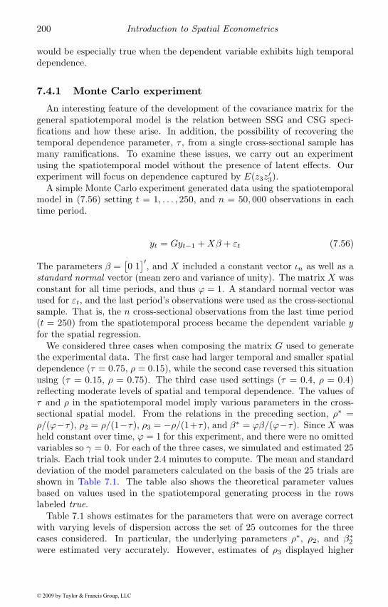
200 Introduction to Spatial Econometrics
would be especially true when the dependent variable exhibits high temporaldependence.
7.4.1 Monte Carlo experiment
An interesting feature of the development of the covariance matrix for thegeneral spatiotemporal model is the relation between SSG and CSG speci-fications and how these arise. In addition, the possibility of recovering thetemporal dependence parameter, τ , from a single cross-sectional sample hasmany ramifications. To examine these issues, we carry out an experimentusing the spatiotemporal model without the presence of latent effects. Ourexperiment will focus on dependence captured by E(z3z′3).
A simple Monte Carlo experiment generated data using the spatiotemporalmodel in (7.56) setting t = 1, . . . , 250, and n = 50, 000 observations in eachtime period.
yt = Gyt−1 +Xβ + εt (7.56)
The parameters β =[0 1
]′, and X included a constant vector ιn as well as astandard normal vector (mean zero and variance of unity). The matrix X wasconstant for all time periods, and thus ϕ = 1. A standard normal vector wasused for εt, and the last period’s observations were used as the cross-sectionalsample. That is, the n cross-sectional observations from the last time period(t = 250) from the spatiotemporal process became the dependent variable yfor the spatial regression.
We considered three cases when composing the matrix G used to generatethe experimental data. The first case had larger temporal and smaller spatialdependence (τ = 0.75, ρ = 0.15), while the second case reversed this situationusing (τ = 0.15, ρ = 0.75). The third case used settings (τ = 0.4, ρ = 0.4)reflecting moderate levels of spatial and temporal dependence. The values ofτ and ρ in the spatiotemporal model imply various parameters in the cross-sectional spatial model. From the relations in the preceding section, ρ∗ =ρ/(ϕ−τ), ρ2 = ρ/(1−τ), ρ3 = −ρ/(1+τ), and β∗ = ϕβ/(ϕ−τ). Since X washeld constant over time, ϕ = 1 for this experiment, and there were no omittedvariables so γ = 0. For each of the three cases, we simulated and estimated 25trials. Each trial took under 2.4 minutes to compute. The mean and standarddeviation of the model parameters calculated on the basis of the 25 trials areshown in Table 7.1. The table also shows the theoretical parameter valuesbased on values used in the spatiotemporal generating process in the rowslabeled true.
Table 7.1 shows estimates for the parameters that were on average correctwith varying levels of dispersion across the set of 25 outcomes for the threecases considered. In particular, the underlying parameters ρ∗, ρ2, and β∗
2
were estimated very accurately. However, estimates of ρ3 displayed higher
© 2009 by Taylor & Francis Group, LLC
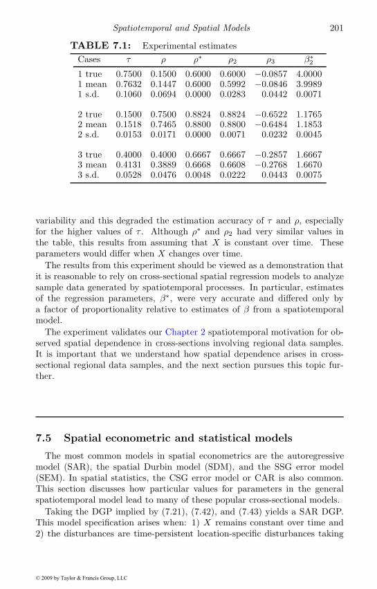
Spatiotemporal and Spatial Models 201
TABLE 7.1: Experimental estimatesCases τ ρ ρ∗ ρ2 ρ3 β∗
2
1 true 0.7500 0.1500 0.6000 0.6000 −0.0857 4.00001 mean 0.7632 0.1447 0.6000 0.5992 −0.0846 3.99891 s.d. 0.1060 0.0694 0.0000 0.0283 0.0442 0.0071
2 true 0.1500 0.7500 0.8824 0.8824 −0.6522 1.17652 mean 0.1518 0.7465 0.8800 0.8800 −0.6484 1.18532 s.d. 0.0153 0.0171 0.0000 0.0071 0.0232 0.0045
3 true 0.4000 0.4000 0.6667 0.6667 −0.2857 1.66673 mean 0.4131 0.3889 0.6668 0.6608 −0.2768 1.66703 s.d. 0.0528 0.0476 0.0048 0.0222 0.0443 0.0075
variability and this degraded the estimation accuracy of τ and ρ, especiallyfor the higher values of τ . Although ρ∗ and ρ2 had very similar values inthe table, this results from assuming that X is constant over time. Theseparameters would differ when X changes over time.
The results from this experiment should be viewed as a demonstration thatit is reasonable to rely on cross-sectional spatial regression models to analyzesample data generated by spatiotemporal processes. In particular, estimatesof the regression parameters, β∗, were very accurate and differed only bya factor of proportionality relative to estimates of β from a spatiotemporalmodel.
The experiment validates our Chapter 2 spatiotemporal motivation for ob-served spatial dependence in cross-sections involving regional data samples.It is important that we understand how spatial dependence arises in cross-sectional regional data samples, and the next section pursues this topic fur-ther.
7.5 Spatial econometric and statistical models
The most common models in spatial econometrics are the autoregressivemodel (SAR), the spatial Durbin model (SDM), and the SSG error model(SEM). In spatial statistics, the CSG error model or CAR is also common.This section discusses how particular values for parameters in the generalspatiotemporal model lead to many of these popular cross-sectional models.
Taking the DGP implied by (7.21), (7.42), and (7.43) yields a SAR DGP.This model specification arises when: 1) X remains constant over time and2) the disturbances are time-persistent location-specific disturbances taking
© 2009 by Taylor & Francis Group, LLC
202 Introduction to Spatial Econometrics
the form we have labeled r, and 3) there are no omitted variables correlatedwith the explanatory variables. These restrictions yield (7.57) and the simplerform shown in (7.58).
y = (In − ρ
1 − τW )−1(1 − τ)−1Xβ +
(In − ρ
1 − τW )−1(1 − τ)−1r (7.57)
y = (In − ρ∗W )−1Xβ∗ + (In − ρ∗W )−1r∗ (7.58)
In the context of a SAR model where y represents variation in home prices,r could capture amenities. These might include water views, tree shade, bikepaths, landscaping, and sidewalks. We might also have externalities reflect-ing proximity to sewerage treatment plants, hazardous waste sites, nearbyhouses with garish, discordant colors, or noise from roads. Other environ-mental factors could include microclimates such as frost pockets, locationson the south or north side of a hill as well as the direction and strength ofwind. Also, Catholic school districts, Catholic parishes, mosquito abatementdistricts, special assessment areas, and parade routes are ignored in most ap-plied modeling situations. Any or all of these serve as examples of potentiallyomitted variables that have a spatial character. In fact, almost every loca-tion is influenced by variables that change slowly over time and the relevantvariables differ across locations.
The SEM or error model DGP in (7.59) arises when the only error compo-nent is r and no omitted variables exist.
y = Xβ + (In − ρ
1 − τW )−1(1 − τ)−1r (7.59)
y = Xβ + (In − ρ∗W )−1r∗ (7.60)
Therefore, the standard SSG error model emerges from a spatiotemporal errorprocess with time-persistent, location-specific disturbances r and no omittedvariables that are correlated with X (i.e., γ = 0). Unlike the autoregres-sive case, X does not need to be constant over time to arrive at this modelspecification.
However, if omitted variables that are correlated with X are present (i.e.,γ �= 0) and no growth in X occurs, this results in a more complicated expres-sion in (7.61).
y = Xβ + (In − ρ
1 − τW )−1X(γ(1 − τ)−1) +
(In − ρ
1 − τW )−1(1 − τ)−1r (7.61)
To estimate (7.61) we can transform y by (In − ρ1−τW ) to yield (7.63) that
has iid disturbances.
© 2009 by Taylor & Francis Group, LLC
Spatiotemporal and Spatial Models 203
(In − ρ
1 − τW )y = (In − ρ
1 − τW )Xβ +
Xγ(1 − τ)−1 + (1 − τ)−1r (7.62)(In − ρ∗W )y = Xβ1 +WXβ2 + r∗ (7.63)
The new equation (7.63) is the SDM. This specification arises when: 1) omit-ted variables that are correlated with X are present (i.e., γ �= 0) and 2) nogrowth in X occurs over time.
Suppose interest centers on an error model with iid disturbances over timewith no omitted variables (γ = 0). Using an earlier expression (7.49) for thecovariance Ωz3 shows that the error model DGP in (7.64) and (7.65) arisesfor large τ (τo).
y = Xβ + ε (7.64)
ε ∼ N(0,Ωz3) ≈ N(0, (1 − τ2o )−1σ2
ε(In − ρ
1 − τoW )−1) (7.65)
Therefore, the standard CSG error model emerges from a spatiotemporal errorprocess with iid disturbances ε, when no omitted variables are present thatare correlated with X (i.e., γ = 0), and τ is large. Unlike the autoregressivecase, X does not need to be constant over time to arrive at this form.
In conclusion, the general spatiotemporal autoregressive and error modelspresented in Sections 7.2 and 7.3 subsume many of the well-known mod-els from spatial econometrics and spatial statistics. Assumptions regardingspecific parameters of the more general model lead to spatial autoregressivemodels (SAR), the spatial Durbin model (SDM), the SSG error model (SEM),and the CSG error model (CAR).
7.6 Patterns of temporal and spatial dependence
Although autoregressive dependence is the most commonly used form oftemporal dependence, other forms exist such as moving average and expo-nential. We provide a brief development that shows how alternative types oftemporal dependence in the context of spatiotemporal processes relate to al-ternative spatial models. In particular, this development suggests that spatialmodels can often inherit the form of the underlying spatiotemporal process.
We begin with a specification in (7.66) that assumes the model variablesare in long-run equilibrium. In the last time period t, the dependent variableyt depends on space-time lags as well as on Xβ and disturbances ut.
© 2009 by Taylor & Francis Group, LLC
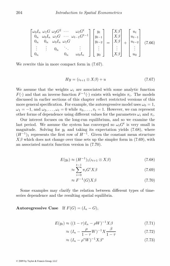
204 Introduction to Spatial Econometrics
⎡⎢⎢⎢⎢⎢⎣ω0In ω1G ω2G
2 · · · ωtGt
0n ω0In ω1G · · · ωt−1Gt−1
0n 0n ω0In ω1G...
... 0n. . .
...0n 0n ω0In
⎤⎥⎥⎥⎥⎥⎦
⎡⎢⎢⎢⎢⎢⎣ytyt−1
yt−2
...y0
⎤⎥⎥⎥⎥⎥⎦ =
⎡⎢⎢⎢⎢⎢⎣XβXβXβ...Xβ
⎤⎥⎥⎥⎥⎥⎦+
⎡⎢⎢⎢⎢⎢⎣utut−1
ut−2
...u0
⎤⎥⎥⎥⎥⎥⎦ (7.66)
We rewrite this in more compact form in (7.67).
Hy = (ιt+1 ⊗Xβ) + u (7.67)
We assume that the weights ωi are associated with some analytic functionF (·) and that an inverse function F−1(·) exists with weights πi. The modelsdiscussed in earlier sections of this chapter reflect restricted versions of thismore general specification. For example, the autoregressive model uses ω0 = 1,ω1 = −1, and ω2, . . . , ωt = 0 while π0, . . . , πt = 1. However, we can representother forms of dependence using different values for the parameters ωi and πi.
Our interest focuses on the long-run equilibrium, and so we examine thelast period. We assume the system has converged so ωtG
t is very small inmagnitude. Solving for yt and taking its expectation yields (7.68), where(H−1)1 represents the first row of H−1. Given the constant mean structureXβ which does not change over time sets up the simpler form in (7.69), withan associated matrix function version in (7.70).
E(yt) ≈ (H−1)1(ιt+1 ⊗Xβ) (7.68)
≈t−1∑i=0
πiGiXβ (7.69)
≈ F−1(G)Xβ (7.70)
Some examples may clarify the relation between different types of time-series dependence and the resulting spatial equilibria.
Autoregressive Case If F (G) = (In −G),
E(yt) ≈ ((1 − τ)In − ρW )−1Xβ (7.71)
≈ (In − ρ
1 − τW )−1X
β
1 − τ(7.72)
≈ (In − ρ∗W )−1Xβ∗ (7.73)
© 2009 by Taylor & Francis Group, LLC
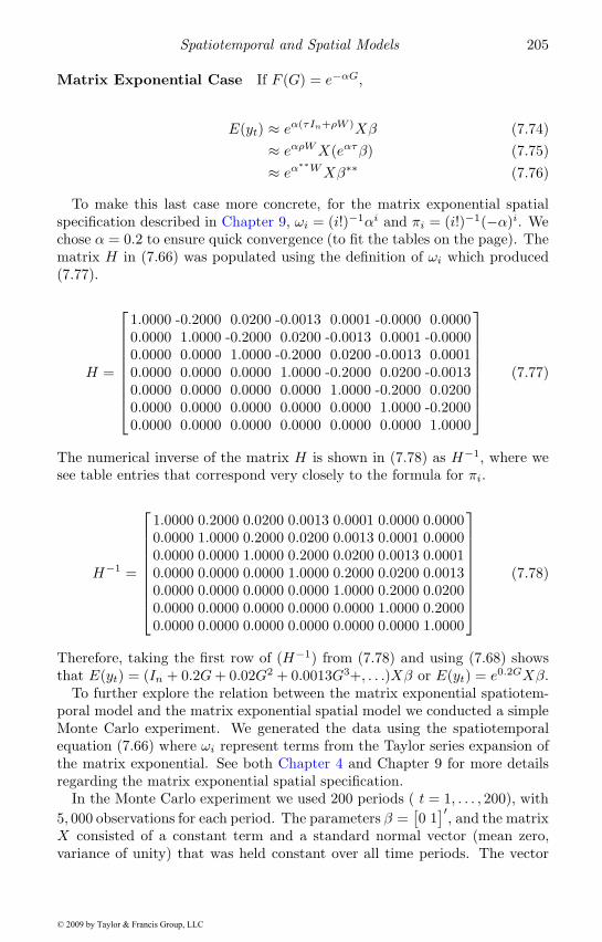
Spatiotemporal and Spatial Models 205
Matrix Exponential Case If F (G) = e−αG,
E(yt) ≈ eα(τIn+ρW )Xβ (7.74)≈ eαρWX(eατβ) (7.75)≈ eα
∗∗WXβ∗∗ (7.76)
To make this last case more concrete, for the matrix exponential spatialspecification described in Chapter 9, ωi = (i!)−1αi and πi = (i!)−1(−α)i. Wechose α = 0.2 to ensure quick convergence (to fit the tables on the page). Thematrix H in (7.66) was populated using the definition of ωi which produced(7.77).
H =
⎡⎢⎢⎢⎢⎢⎢⎢⎢⎣
1.0000 -0.2000 0.0200 -0.0013 0.0001 -0.0000 0.00000.0000 1.0000 -0.2000 0.0200 -0.0013 0.0001 -0.00000.0000 0.0000 1.0000 -0.2000 0.0200 -0.0013 0.00010.0000 0.0000 0.0000 1.0000 -0.2000 0.0200 -0.00130.0000 0.0000 0.0000 0.0000 1.0000 -0.2000 0.02000.0000 0.0000 0.0000 0.0000 0.0000 1.0000 -0.20000.0000 0.0000 0.0000 0.0000 0.0000 0.0000 1.0000
⎤⎥⎥⎥⎥⎥⎥⎥⎥⎦(7.77)
The numerical inverse of the matrix H is shown in (7.78) as H−1, where wesee table entries that correspond very closely to the formula for πi.
H−1 =
⎡⎢⎢⎢⎢⎢⎢⎢⎢⎣
1.0000 0.2000 0.0200 0.0013 0.0001 0.0000 0.00000.0000 1.0000 0.2000 0.0200 0.0013 0.0001 0.00000.0000 0.0000 1.0000 0.2000 0.0200 0.0013 0.00010.0000 0.0000 0.0000 1.0000 0.2000 0.0200 0.00130.0000 0.0000 0.0000 0.0000 1.0000 0.2000 0.02000.0000 0.0000 0.0000 0.0000 0.0000 1.0000 0.20000.0000 0.0000 0.0000 0.0000 0.0000 0.0000 1.0000
⎤⎥⎥⎥⎥⎥⎥⎥⎥⎦(7.78)
Therefore, taking the first row of (H−1) from (7.78) and using (7.68) showsthat E(yt) = (In + 0.2G+ 0.02G2 + 0.0013G3+, . . .)Xβ or E(yt) = e0.2GXβ.
To further explore the relation between the matrix exponential spatiotem-poral model and the matrix exponential spatial model we conducted a simpleMonte Carlo experiment. We generated the data using the spatiotemporalequation (7.66) where ωi represent terms from the Taylor series expansion ofthe matrix exponential. See both Chapter 4 and Chapter 9 for more detailsregarding the matrix exponential spatial specification.
In the Monte Carlo experiment we used 200 periods ( t = 1, . . . , 200), with5, 000 observations for each period. The parameters β =
[0 1
]′, and the matrixX consisted of a constant term and a standard normal vector (mean zero,variance of unity) that was held constant over all time periods. The vector
© 2009 by Taylor & Francis Group, LLC
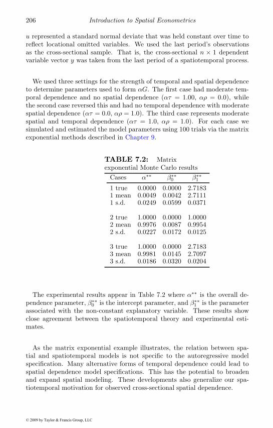
206 Introduction to Spatial Econometrics
u represented a standard normal deviate that was held constant over time toreflect locational omitted variables. We used the last period’s observationsas the cross-sectional sample. That is, the cross-sectional n × 1 dependentvariable vector y was taken from the last period of a spatiotemporal process.
We used three settings for the strength of temporal and spatial dependenceto determine parameters used to form αG. The first case had moderate tem-poral dependence and no spatial dependence (ατ = 1.00, αρ = 0.0), whilethe second case reversed this and had no temporal dependence with moderatespatial dependence (ατ = 0.0, αρ = 1.0). The third case represents moderatespatial and temporal dependence (ατ = 1.0, αρ = 1.0). For each case wesimulated and estimated the model parameters using 100 trials via the matrixexponential methods described in Chapter 9.
TABLE 7.2: Matrixexponential Monte Carlo results
Cases α∗∗ β∗∗0 β∗∗
1
1 true 0.0000 0.0000 2.71831 mean 0.0049 0.0042 2.71111 s.d. 0.0249 0.0599 0.0371
2 true 1.0000 0.0000 1.00002 mean 0.9976 0.0087 0.99542 s.d. 0.0227 0.0172 0.0125
3 true 1.0000 0.0000 2.71833 mean 0.9981 0.0145 2.70973 s.d. 0.0186 0.0320 0.0204
The experimental results appear in Table 7.2 where α∗∗ is the overall de-pendence parameter, β∗∗
0 is the intercept parameter, and β∗∗1 is the parameter
associated with the non-constant explanatory variable. These results showclose agreement between the spatiotemporal theory and experimental esti-mates.
As the matrix exponential example illustrates, the relation between spa-tial and spatiotemporal models is not specific to the autoregressive modelspecification. Many alternative forms of temporal dependence could lead tospatial dependence model specifications. This has the potential to broadenand expand spatial modeling. These developments also generalize our spa-tiotemporal motivation for observed cross-sectional spatial dependence.
© 2009 by Taylor & Francis Group, LLC
Spatiotemporal and Spatial Models 207
7.7 Chapter summary
This chapter dealt with spatiotemporal models as well as the relation be-tween spatial and spatiotemporal models. We began with Section 7.1 andshowed that the well-known partial adjustment model can be easily augmentedto include previous values of the dependent and explanatory variables fromnearby observations or regions. This results in a spatiotemporal model thatcontains both time as well as space-time lags of the model variables, but nocontemporaneous spatial lags.
In Section 7.2 we introduced a general spatiotemporal autoregressive pro-cess involving explanatory variables with deterministic growth, temporal lagsof variables, temporal lags of spatial lags of variables, and a disturbance termcomprised of three components. One component was a locational omittedvariable (not correlated with the included variables), the second componentwas an omitted variable correlated with the included variables, and the thirdcomponent was an iid disturbance.
Although this was a more general process, it did not contain any form ofsimultaneous spatial dependence in the spatiotemporal process itself as thiswould be assuming what we are trying to demonstrate (how simultaneousspatial dependence arises).
We showed that the resulting long-run equilibrium arising from this strictspatiotemporal process took the form: E(yt) ≈ (In − ρ∗W )−1Xtβ
∗, whereρ∗ = ρ(ϕ − τ)−1, and β∗ = (β + γ)ϕ(ϕ − τ)−1. The scalar ρ is the spatialdependence parameter, τ is the temporal dependence parameter, γ reflectsdependence between the included and omitted variable, and ϕ equals 1 plusthe growth rate of X over time.
The relation between the long-run equilibrium parameters and the spa-tiotemporal model parameters has important implications concerning the in-terpretation and use of these models. In particular, cross-sectional spatialregressions and spatiotemporal regressions could produce very different esti-mates of dependence even when both types of models are correctly specified.For example, a cross-sectional spatial regression could result in estimates in-dicating high spatial dependence while a spatiotemporal regression could pro-duce estimates indicating relatively high temporal dependence and low spatialdependence. Despite the fact that the estimates from these two types of mod-els are seemingly quite different, both regressions could be correct since theyare based on different information sets. In some applications, a large andsignificant temporal parameter estimate coupled with a small and less sig-nificant spatial parameter estimate could entice a practitioner into deletingthe spatial variable. Although this strategy may seem fine from a goodness-of-fit perspective, interpretation of the two models would differ greatly. Asmall spatial parameter estimate and large temporal parameter estimate ina spatiotemporal model implies a long-run equilibrium with material spatial
© 2009 by Taylor & Francis Group, LLC
208 Introduction to Spatial Econometrics
dependence, whereas a purely temporal regression implies a long-run equilib-rium with no spatial dependence. This would make a large difference in howwe interpret the impacts arising from changes in the explanatory variables ofthe model.
Section 7.3 showed a similar analysis for a spatiotemporal error modelwhere, in the absence of omitted variables correlated with the included vari-ables, the long-run equilibrium resulted in E(yt) ≈ Xtβ. Although the dis-turbances exhibit spatial dependence, the actual long-run equilibrium is non-spatial. However, in the presence of omitted variables correlated with includedvariables, the error model yields a form of SDM, and this is fundamentally aspatial model.
Section 7.4 addressed the form of covariance structure that arises fromusing a spatiotemporal process to motivate a cross-sectional model specifica-tion. This development considered the case where the disturbances consistedof components related to a locational omitted variable as well as iid distur-bances. Various parameter combinations resulted in CSG and SSG covariancestructures. In particular, the presence of time-persistent, spatially dependentdisturbances and high levels of time dependence τ yield the SSG covariancestructure.
Section 7.4.1 provided a Monte Carlo demonstration that the CSG specifi-cation can arise in the presence of strong temporal dependence as discussed inSection 7.4. Under the correct model specification, the regression parameterswere well estimated by a purely spatial model and comparable (proportion-ally) to those estimated from a spatiotemporal model using panel data. TheMonte Carlo experiment corroborated the relation between the spatial andspatiotemporal approaches. However, for actual data the relation betweenthese may be difficult to confirm as these relations take the form of ratios andare very sensitive to minor estimation errors, especially those pertaining tothe temporal parameter τ .
Section 7.6 showed how specific assumptions within the general spatiotem-poral framework could lead to standard cross-sectional spatial models. Weshowed that other temporal DGPs such as the matrix exponential processalso implied various spatial long-run equilibria. This provides a means ofextending various results from time series analysis to spatial econometrics.
The relation between spatiotemporal and spatial models motivates somemodeling strategies. First, economic theory underlies many time series modelsand these may have spatial analogs. Therefore, theory may suggest morespecific functional forms.
Second, allowing for growth in the explanatory variablesX over time impliesthat the dependence parameter governing the mean could differ from thedependence parameter governing the covariance structure of the model. Forexample, in the spatial autoregressive model that allows X to grow over timethe DGP is: y = (In− ρaW )−1Xβ+ (In− ρbW )−1r. Only the special case inwhich X is constant over time leads to ρa = ρb. In large samples, efficiencybecomes less of an issue relative to bias, and so getting the mean part of the
© 2009 by Taylor & Francis Group, LLC
Spatiotemporal and Spatial Models 209
model correct (i.e., E(yt) = F−1(G)Xβ) becomes more important and greatlyaffects model interpretation.
More generally, the processes governing X over time enter into the form ofthe spatial model. This suggests more elaborate lag structures involving theexplanatory variables. For example, variants of the SDM that involve someform of distributed lags might be considered (Byron, 1992).
A third implication for modeling strategy would be that the covariancestructure may be more complicated than in the standard models. Althoughmodeling covariance may not be as important in large samples, it obviouslyaffects the validity of inference for marginal variables and could aid in predic-tion as well as imputation.
Finally, using different parameters for modeling the mean of the processversus the disturbance process should provide some insurance against con-tamination of the mean model parameters that can arise from misspecificationof the disturbance process. As discussed in Chapter 3 in the context of theHausman test, misspecification of the model for the disturbance process willnot affect parameter estimates associated with the (correctly specified) meanmodel in large samples. Therefore, using different parameters to specify themodel for the mean versus the model for the disturbances may lead to morerobust spatial modeling. The SDEM introduced in Section 2.7 represents oneof the simplest models with this property.
The development here should also benefit the literature on space-time paneldata models. This literature relies on traditional spatial regression modelsaugmented with random effects parameters and space-time covariance struc-tures. Using spatiotemporal processes of the type explored here could makethese models more intuitive. This would ensure that space-time panel modelspecifications could be justified as arising from underlying space-time inter-actions that evolve over time to a steady state equilibrium. It would alsopromote understanding of the properties associated with the observed panelof cross-sectional sample data used to estimate the parameters of these mod-els.
© 2009 by Taylor & Francis Group, LLC
Chapter 8
Spatial Econometric InteractionModels
Gravity models have often been used to explain origin-destination (OD) flowsthat arise in fields such as international and regional trade, transportationeconomics, population migration research, modeling of commodity flows, com-munication and other types of information flows along a network and journey-to-work studies.
A large literature on theoretical foundations for these models in the specificcontext of international trade models exists (Anderson, 1979; Anderson andvan Wincoop, 2004). In the regional science literature the gravity modelhas been labeled a spatial interaction model (Sen and Smith, 1995), becausethe regional interaction is directly proportional to the product of regionalsize measures. In the case of interregional commodity flows, the measure ofregional size is typically gross regional product or regional income. The modelpredicts more interaction in the form of commodity flows between regions ofsimilar (economic) size than regions dissimilar in size. In other contexts suchas knowledge flows between regions (LeSage, Fischer and Scherngell, 2007)the size measure of regions might be the stock of patents, so that regions withsimilar knowledge stocks would exhibit more spatial interaction taking theform of knowledge flows.
These models rely on a function of the distance between an origin and des-tination as well as explanatory variables pertaining to characteristics of bothorigin and destination regions. Spatial interaction models assume that us-ing distance as an explanatory variable will eradicate the spatial dependenceamong the sample of OD flows between pairs of regions. The notion thatuse of distance functions in conventional spatial interaction models effectivelycaptures spatial dependence in interregional flows has long been challenged.Griffith (2007) provides an historical review of regional science literature onthis topic in which he credits Curry (1972) as the first to conceptualize theproblem of spatial dependence in flows. Griffith and Jones (1980) in a studyof Canadian journey-to-work flows noted that flows from an origin are “en-hanced or diminished in accordance with the propensity of emissiveness of itsneighboring origin locations.” They also stated that flows associated with adestination are “enhanced or diminished in accordance with the propensity ofattractiveness of its neighboring destination locations.”
LeSage and Pace (2008) make the point that assuming independence be-
211© 2009 by Taylor & Francis Group, LLC
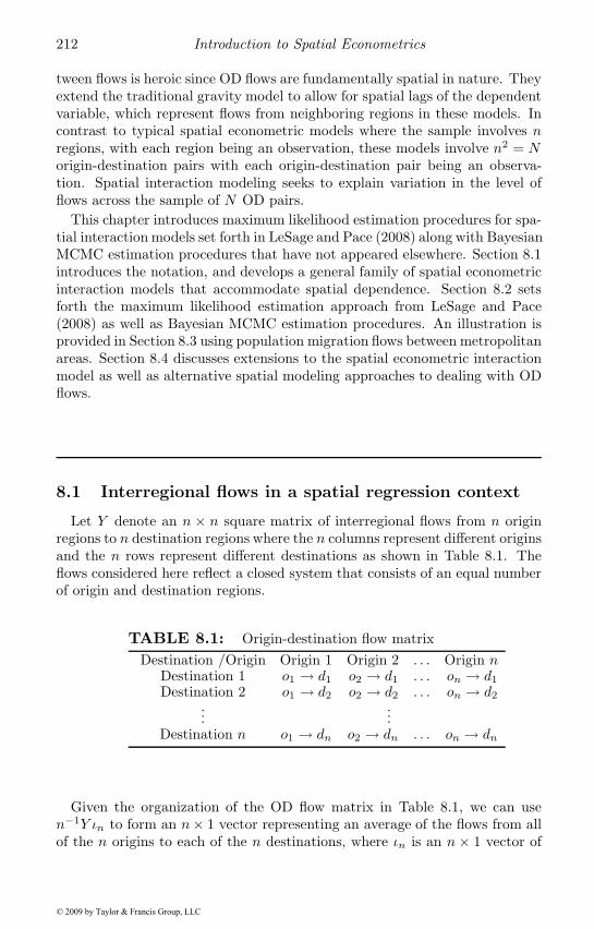
212 Introduction to Spatial Econometrics
tween flows is heroic since OD flows are fundamentally spatial in nature. Theyextend the traditional gravity model to allow for spatial lags of the dependentvariable, which represent flows from neighboring regions in these models. Incontrast to typical spatial econometric models where the sample involves nregions, with each region being an observation, these models involve n2 = Norigin-destination pairs with each origin-destination pair being an observa-tion. Spatial interaction modeling seeks to explain variation in the level offlows across the sample of N OD pairs.
This chapter introduces maximum likelihood estimation procedures for spa-tial interaction models set forth in LeSage and Pace (2008) along with BayesianMCMC estimation procedures that have not appeared elsewhere. Section 8.1introduces the notation, and develops a general family of spatial econometricinteraction models that accommodate spatial dependence. Section 8.2 setsforth the maximum likelihood estimation approach from LeSage and Pace(2008) as well as Bayesian MCMC estimation procedures. An illustration isprovided in Section 8.3 using population migration flows between metropolitanareas. Section 8.4 discusses extensions to the spatial econometric interactionmodel as well as alternative spatial modeling approaches to dealing with ODflows.
8.1 Interregional flows in a spatial regression context
Let Y denote an n × n square matrix of interregional flows from n originregions to n destination regions where the n columns represent different originsand the n rows represent different destinations as shown in Table 8.1. Theflows considered here reflect a closed system that consists of an equal numberof origin and destination regions.
TABLE 8.1: Origin-destination flow matrixDestination /Origin Origin 1 Origin 2 . . . Origin n
Destination 1 o1 → d1 o2 → d1 . . . on → d1
Destination 2 o1 → d2 o2 → d2 . . . on → d2
......
Destination n o1 → dn o2 → dn . . . on → dn
Given the organization of the OD flow matrix in Table 8.1, we can usen−1Y ιn to form an n× 1 vector representing an average of the flows from allof the n origins to each of the n destinations, where ιn is an n× 1 vector of
© 2009 by Taylor & Francis Group, LLC
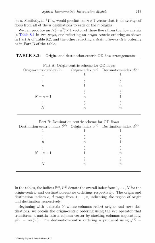
Spatial Econometric Interaction Models 213
ones. Similarly, n−1Y ′ιn would produce an n× 1 vector that is an average offlows from all of the n destinations to each of the n origins.
We can produce an N(= n2)× 1 vector of these flows from the flow matrixin Table 8.1 in two ways, one reflecting an origin-centric ordering as shownin Part A of Table 8.2, and the other reflecting a destination-centric orderingas in Part B of the table.
TABLE 8.2: Origin- and destination-centric OD flow arrangements
Part A: Origin-centric scheme for OD flowsOrigin-centric index l(o) Origin-index o(o) Destination-index d(o)
1 1 1...
......
n 1 n...
......
N − n+ 1 n 1...
......
N n n
Part B: Destination-centric scheme for OD flowsDestination-centric index l(d) Origin-index o(d) Destination-index d(d)
1 1 1...
......
n n 1...
......
N − n+ 1 1 n...
......
N n n
In the tables, the indices l(o), l(d) denote the overall index from 1, . . . , N for theorigin-centric and destination-centric orderings respectively. The origin anddestination indices o, d range from 1, . . . , n, indicating the region of originand destination respectively.
Beginning with a matrix Y whose columns reflect origins and rows des-tinations, we obtain the origin-centric ordering using the vec operator thattransforms a matrix into a column vector by stacking columns sequentially,y(o) = vec(Y ). The destination-centric ordering is produced using y(d) =
© 2009 by Taylor & Francis Group, LLC
214 Introduction to Spatial Econometrics
vec(Y ′). These two orderings are related by the vec-permutation matrix Pso that Py(o) = y(d). Based on the properties of permutation matrices, it isalso true that y(o) = P−1y(d) = P ′y(d). For our discussion in this chapterwe will focus on the origin-centric ordering where the first n elements in thestacked vector y(o) reflect flows from origin 1 to all n destinations. The lastn elements of this vector represent flows from origin n to destinations 1 ton. We will refer to this OD flow vector as simply y, which represents thedependent variable vector in our spatial econometric interaction model.
A conventional gravity or spatial interaction model relies on a single vectoror an n × k matrix of explanatory variables that we label X , containing kcharacteristics for each of the n regions. The matrix X is repeated n timesto produce an N × k matrix representing destination characteristics that welabel Xd. LeSage and Pace (2008) note that Xd equals ιn ⊗ X , where ιn isan n × 1 vector of ones. A second matrix can be formed to represent origincharacteristics that we label Xo. This would repeat the characteristics of thefirst region n times to form the first n rows of Xo, the characteristics of thesecond region n times for the next n rows of Xo and so on, resulting in anN×k matrix that we label Xo = X⊗ ιn. International trade models typicallyrely on a single explanatory variable vector X such as income to reflect thesize of regions. This would result in N×1 vectorsXd, Xo rather than matricesof explanatory variables.
We note that the vec-permutation matrix P can be used to translate be-tween origin-centric and destination-centric ordering of the sample data. Forexample, if we adopted the destination-centric ordering (as opposed to theorigin-centric ordering), specification of the destination explanatory variablesmatrix would be X
(d)d = X ⊗ ιn. This can be seen using the relation:
P ′XdP = P ′(ιn ⊗ X)P = X(d)d , to translate the origin-centric destination
covariates Xd to the destination-centric ordering scheme X(d)d . Rules for
multiplication using Kronecker products allow us to simplify the expressionP ′(ιn ⊗ X)P , (Horn and Johnson, 1994, Corollary 4.3.10, p. 260), so thatP ′(ιn⊗X)P = X⊗ ιn, and thus X(d)
d = X⊗ ιn, under the destination-centricordering of the sample data.
The distance from each origin to destination is also included as an explana-tory variable vector in the gravity model. If we let G represent the n × nmatrix of distances between origins and destinations, g = vec(G) is an N × 1vector of distances from each origin to each destination formed by stackingthe columns of the origin-destination distance matrix into a variable vector.
This results in a regression model of the type shown in (8.1). This isidentical to the model that arises when applying a log transformation to thestandard gravity model (Sen and Smith, 1995, c.f., equation (6.4)).
y = αιN +Xdβd +Xoβo + γg + ε (8.1)The vectors βd and βo are k× 1 parameter vectors associated with the des-
tination and origin region characteristics. If a log transformation is applied to
© 2009 by Taylor & Francis Group, LLC
Spatial Econometric Interaction Models 215
the dependent variable y and explanatory variables matrix X , the coefficientestimates would reflect elasticity responses of OD flows to the various originand destination characteristics. The scalar parameter γ reflects the effect ofdistance g, and α denotes the constant term parameter. The N × 1 vector εhas a zero mean, constant variance and zero covariance between disturbances.
LeSage and Pace (2008) propose a spatial autoregressive extension of thenon-spatial model in (8.1) shown in (8.2). This model can be viewed asfiltering for spatial dependence related to the destination and origin regions.
(IN − ρdWd)(IN − ρoWo)y = αιN +Xdβd +Xoβo + γg + ε (8.2)
The N ×N matrix Wd is constructed from the typical row-stochastic n×nmatrix W that describes spatial connectivity between the n regions. Weassume that W is similar to a symmetric matrix so that it has real eigenvaluesand n orthogonal eigenvectors. The matrix Wd can be written using theKronecker product shown in (8.3).
Wd = In ⊗W =
⎛⎜⎜⎜⎜⎜⎜⎜⎝
W 0n . . . . . . 0n
0n W...
... W. . .
0n . . . W
⎞⎟⎟⎟⎟⎟⎟⎟⎠(8.3)
The motivation for this construction is given by the origin-centric notationfrom Table 8.2. Let Y1 be origin-destination flows from the first origin to alldestinations. The spatial lag WY1 would then contain a spatial average offlows from this origin to neighbors of each destination i = 1, . . . , n. Similarly,the spatial lag WY2 would produce a spatial average of flows from the secondorigin to neighbors of each destination, and so on. This motivates use of theKronecker product to repeat the spatial lags n times, resulting in an N ×Nspatial weight matrix that captures destination-based dependence.
This type of dependence reflects the intuition that forces leading to flowsfrom an origin to a destination may create similar flows to nearby or neigh-boring destinations, which is captured by the spatial lag created using thematrix-vector product Wdy. This spatial lag formally captures the notion setforth in Griffith and Jones (1980) that flows associated with a destination are“enhanced or diminished in accordance with the propensity of attractivenessof its neighboring destination locations.”
Taking a similar approach to that used in developing the matrix Wd, wecan also create an N × N row-standardized spatial weight matrix that welabel Wo = W ⊗ In. This follows by noting that W (Y ′
1) provides spatialaverages around each origin of flows to the first destination. Doing this for alldestinations yields WY ′, and vec(WY ′) = (W ⊗ In)vec(Y ) = (W ⊗ In)y. The
© 2009 by Taylor & Francis Group, LLC
216 Introduction to Spatial Econometrics
spatial lag formed by the matrix product Woy = (W ⊗ In)y captures origin-based spatial dependence using an average of flows from neighbors to the originregions to each of the destinations. This type of dependence reflects the notionthat forces leading to flows from any origin to a particular destination regionmay create similar flows from nearby neighboring origins. The spatial lagWoy formally captures the point of Griffith and Jones (1980) that flows froman origin are “enhanced or diminished in accordance with the propensity ofemissiveness of its neighboring origin locations.”
As already noted for the case of the explanatory variables matrices, thevec-permutation matrix P can be used to translate between origin-centricand destination-centric ordering of the sample data. For example, if we adoptthe destination-centric ordering (as opposed to the origin-centric ordering usedhere), specification of the destination weight matrix would be W (d)
d = W ⊗In.As in the case of the matrix Xd, we can use the relation: P ′WdP = P ′(In ⊗W )P = W ⊗ In = W
(d)d , to produce the destination weight matrix for the
destination-centric ordering scheme.The model in (8.2) is motivated by the fact that both types of dependence
are likely to exist in our spatial specification for origin-destination flows. Thismodel can be viewed as a successive spatial filter that filters the OD flows iny successively by (IN − ρdWd) and (IN − ρoWo). Remarkably one can changethe order in which the filter is applied and arrive at the same model. That is,we could remove origin dependence first and destination dependence second,using the filter (IN − ρoWo)(IN − ρdWd). This is true because the cross-product term (W ⊗ In)(In ⊗W ) = W ⊗W is the same as the cross-product(In ⊗W )(W ⊗ In) via the mixed-product rule for Kronecker products.
Expanding the product (IN − ρdWd)(IN − ρoWo) = IN − ρdWd − ρoWo +ρdρoWd · Wo = IN − ρdWd − ρoWo − ρwWw, leads us to consider a thirdtype of dependence reflected in the product Ww = Wo · Wd = (In ⊗ W ) ·(W ⊗ In) = W ⊗W .1 This spatial weight matrix reflects an average of flowsfrom neighbors to the origin to neighbors of the destination, which LeSageand Pace (2008) label origin-to-destination dependence to distinguish it fromorigin-based dependence and destination-based dependence.
This leads LeSage and Pace (2008) to propose the general spatial autore-gressive interaction model in (8.4) that takes into account origin, destination,and origin-to-destination dependence.
y = ρdWdy + ρoWoy + ρwWwy + αιN +Xdβd +Xoβo + γg + ε (8.4)
The omitted variables and space-time dynamic motivations used to producespatial regression models that contain spatial lags of the dependent variables
1We note that this specification implies a restriction that ρw = −ρoρd, but this restrictionneed not be enforced in applied work. Of course, restrictions on the values of the scalardependence parameters ρd, ρo, ρw must be imposed to ensure stationarity in the case whereρw is free of the restriction.
© 2009 by Taylor & Francis Group, LLC
Spatial Econometric Interaction Models 217
set forth in Chapter 2 and Chapter 7 also apply to this model. One can beginwith a non-spatial theoretical relationship such as the utility theory used tomotivate non-spatial interaction models for migration, or the monopolisticcompetition model in conjunction with a CES utility function used to derivea non-spatial gravity equation for trade flows. If we posit the existence ofomitted variables that exhibit spatial dependence and are correlated withincluded variables, a model such as (8.4) that contains spatial lags of thedependent variable (as well as the explanatory variables) will arise. Thatis, an SDM variant of the model in (8.4) could be appropriate for spatialeconometric modeling of OD flows. Similarly, a space-time dynamic can beused to motivate the model in (8.4) as the long-run steady state equilibriumof a process where OD flows exhibit time dependence as well as space-timedependence.
In the trade literature, Anderson and van Wincoop (2004) argue that itis important to include interaction terms that capture the fact that bilateraltrade flows depend not only on bilateral barriers to trade, but also on tradebarriers across all trading partners. Trade barriers or multilateral trade resis-tance are usually modeled as arising from price differentials between regionstaking the form of ‘cost-in-freight’ (c.i.f.) and ‘free-on-board’ (f.o.b.) prices atthe destination and origin regions. The argument is essentially that bilateralpredictions do not readily extend to a multilateral world because these ignoreindirect interactions that link all trading partners. Also of note is the workof Behrens, Ertur and Koch (2007) who extend the monopolistic competitionmodel in conjunction with a CES utility function to derive a gravity equationfor trade flows that contains spatial lags of the dependent variable. They ac-complish this using a quantity-based version of the CES model and exploitingthe fact that price indices (that represent multilateral resistance to trade) im-plicitly depend on trade flows. This in conjunction with the fact that bilateraltrade flows in their model depend on flows from all other trading partners,leads to a model that displays a spatial autoregressive structure in trade flows.Intuitively, they argue that when goods are gross substitutes, trade flows fromany origin to a particular destination will depend on the entire distributionof bilateral trade barriers (prices of substitute goods).
A problem that plagues the empirical trade literature is the lack of reli-able regional price information, (Anderson and van Wincoop, 2004). Becauseof this, Anderson and van Wincoop (2004) suggest a non-statistical compu-tational approach to replace the unobservable prices. As we have alreadymotivated, the presence of latent unobservable variables that exhibit spatialdependence would lead to a model of the type in (8.4) which accounts for theunobserved variables using spatial lags of the dependent variable.
LeSage and Pace (2008) point out that this general model leads to ninemore specific models that may be of interest in empirical work. We enumeratefour of these models that result from various restrictions on the parametersρi, i = d, o, w. The model comparison methods from Chapter 6 could be usedto test these parameter restrictions. However, the nested nature of the family
© 2009 by Taylor & Francis Group, LLC
218 Introduction to Spatial Econometrics
of nine models associated with the parameter restrictions allows the use ofconventional likelihood ratio tests. The four models are enumerated below.
Non-spatial model. The restriction: ρd = ρo = ρw = 0 produces thenon-spatial model where no spatial autoregressive dependence exists.
Model 1. The restriction: ρw = 0 leads to a model with separableorigin and destination autoregressive dependence embodied in the twoweight matrices Wd andWo, while ruling out origin-to-destination baseddependence between neighbors of the origin and destination locationsthat would be captured by Ww.
Model 2. The restriction: ρw = −ρdρo results in a successive filteringmodel involving both origin Wd, and destination Wo dependence as wellas product separable interaction Ww, constrained to reflect the filter(IN − ρdWd)(IN − ρoWo) = (IN − ρoWo)(IN − ρdWd) = (IN − ρdWd −ρoWo + ρdρoWw).
Model 3. The unrestricted model shown in (8.4) involves three matricesWd, Wo, and Ww, which represents the most general member of thefamily of models. Appropriate restrictions on ρd, ρo, and ρw can thusproduce the other more specialized models.
8.2 Maximum likelihood and Bayesian estimation
The likelihood provides the starting point for both maximum likelihood andBayesian estimation. We note that the concentrated log-likelihood functionfor the model specifications will take the form in (8.5).
lnL = κ+ ln |IN − ρdWd − ρoWo − ρwWw| − N
2ln(S(ρd, ρo, ρw)) (8.5)
where S(ρd, ρo, ρw) represents the sum of squared errors expressed as a func-tion of the scalar dependence parameters alone after concentrating out theparameters α, βo, βd, γ and σ2, and the constant κ that does not depend onρd, ρo, ρw (LeSage and Pace, 2008).
LeSage and Pace (2008) show that the log-determinant of the N×N matrixthat appears in (8.5) can be calculated using only traces of the n×nmatrixW ,which greatly simplifies estimation of these models (see Chapter 4). Furthercomputational savings can be achieved by noting that we need not reproducethe n × k data matrix X using the Kronecker products ιn ⊗ X,X ⊗ ιn, ifwe exploit the special structure of this model. The algebra of Kroneckerproducts can be used to form moment matrices without dealing directly with
© 2009 by Taylor & Francis Group, LLC
Spatial Econometric Interaction Models 219
N by N matrices. Given arbitrary, conformable matrices A, B, C, then(C′ ⊗A)vec(B) = vec(ABC) (Horn and Johnson, 1994, Lemma 4.3.1, p. 254-255). Using Z =
(ιN Xd Xo g
)yields the moment matrix Z ′Z shown in
(8.6), where the symbol 0k denotes a 1 × k vector of zeros.2
Z ′Z =
⎛⎜⎜⎝N 0k 0k ι′nGιn0′k nX ′X 0′k0k X ′Gιn0′k 0′k0k nX ′X X ′Gιn
ι′nGιn ι′nG′X ι′nG′X tr(G2)
⎞⎟⎟⎠ (8.6)
Using the algebra of Kronecker products also allows us to avoid forming theN byN matricesWd, Wo, orWw. SinceWdy = (In⊗W )vec(Y ), it follows thatWdy = vec(WY ), using the relation, (C′ ⊗A)vec(B) = vec(ABC). Similarly,Woy = vec(YW ′), andWwy = vec(WYW ′). We use these forms to rewrite themodel from (8.4) as shown in (8.7), where E is an n×n matrix of theoreticaldisturbances.
vec(Y )−ρd vec(WY )−ρo vec(YW ′)−ρw vec(WYW ′) = Zδ+vec(E) (8.7)
The expression on the left-hand-side of (8.7) is a linear combination of fourcomponents, one involving the dependent variable vector vec(Y ), and theother three representing spatial lags of this vector that reflect destination-based dependence vec(WY ), origin-based dependence vec(YW ′) as well asorigin-to-destination based dependence, vec(WYW ′). This allows us to ex-press the parameter estimates as a linear combination of four separate com-ponents which we label δ(t) = (Z ′Z)−1Z ′ vec(F (t)(Y )), where F (t)(Y ) equalsY , WY , YW ′, or WYW ′ when t = 1, . . . , 4. These components can be usedto determine the parameter estimate δ using (8.8).
δ =(δ(1) δ(2) δ(3) δ(4)
)⎛⎜⎜⎝1
−ρd−ρo−ρw
⎞⎟⎟⎠ (8.8)
We can use the expressions δ(t) for t = 1, . . . , 4, to write these terms asa function of the sample data X and Y and the parameters ρd, ρo, ρw. Thisallows us to concentrate the log-likelihood with respect to the parameters δ(t),which contain the parameters α, βd, βo, γ associated with the model covariates.
Component residual matrices E(t), t = 1, . . . , 4 that take the form shown in(8.9) can be used to express the overall residual matrix E = E(1) − ρdE
(2) −ρoE
(3) − ρwE(4) related to the concentrated log-likelihood function.
2We note that this log-likelihood function can be used for the SDM model by replacing thecovariate matrix Z with Z =
(ιN Xd Xo WdXd WoXo g
)in the expressions set forth in
the text.
© 2009 by Taylor & Francis Group, LLC
220 Introduction to Spatial Econometrics
E(t) = F (t)(Y ) − α(t)ιnι′n −Xβ
(t)d ι′n − ιn(β(t)
o )′X ′ − γ(t)G (8.9)
For the purpose of maximizing the log-likelihood we introduce the cross-product matrixQ that consists of various component residual matrices. DefineQij = tr(E(i)′ E(j)), i = 1, . . . , 4, j = 1, . . . , 4, so the sum-of-squared residu-als for our model become S(ρd, ρo, ρw) = τ(ρd, ρo, ρw)′Qτ(ρd, ρo, ρw), whereτ(ρd, ρo, ρw) =
(1 −ρd −ρo −ρw
)′.Consequently, recomputing S(ρd, ρo, ρw) for any set of values
(ρd ρo ρw
)requires a small number of operations that do not depend on n or k. This inconjunction with pre-computed values for the log-determinant term also ex-pressed as a function of these parameters calculated using the efficient meth-ods set forth in LeSage and Pace (2008) permits rapid optimization of thelikelihood function with respect to these parameters. Using a 2.0 Ghz. IntelCore 2 Duo laptop computer it takes around 5 seconds to maximize the log-likelihood function for a problem involving migration flows between n = 359(N = 128, 881) US metropolitan areas.
The Bayesian Markov Chain Monte Carlo (MCMC) estimation proceduresfor standard spatial regression models set forth in Chapter 5 can be appliedto these models. This allows us to extend the model in two useful ways. First,we can accommodate fat-tailed disturbance distributions using our spatial au-toregressive model extension of the non-spatial model introduced by Geweke(1993) discussed in Chapter 5. Second, we can deal with a common problemthat arises in modeling OD flows where many of the flows associated withOD pairs take on zero values. In Chapter 10, we discuss spatial Tobit modelswhere zero observations of the dependent variable are viewed as arising froma sample truncation process. In the context of spatial econometric interactionmodels we could view zero flows as indicative of negative utility (or profits)associated with flows between these particular OD pairs. For example, the ab-sence of migration flows between origin-destination pairs might be indicativeof negative utility arising from moves between these locations.
Turning to Bayesian robust estimation of the spatial econometric interactionmodel, we introduce a set of latent variance scalars for each observation. Thatis, we replace ε ∼ N(0, σ2IN ), with:
ε ∼ N [0, σ2V ] (8.10)Vii = Vi, i = 1, . . . , NV = vec(R)
R =
⎛⎜⎜⎜⎝v11 v12 . . . v1nv21 v22 v2n...
. . .vn1 vnn
⎞⎟⎟⎟⎠
© 2009 by Taylor & Francis Group, LLC
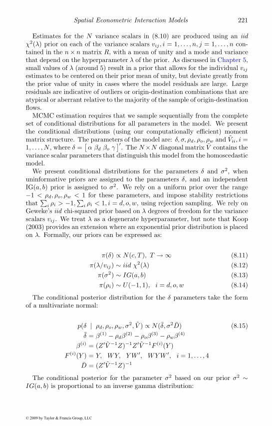
Spatial Econometric Interaction Models 221
Estimates for the N variance scalars in (8.10) are produced using an iidχ2(λ) prior on each of the variance scalars vij , i = 1, . . . , n, j = 1, . . . , n con-tained in the n× n matrix R, with a mean of unity and a mode and variancethat depend on the hyperparameter λ of the prior. As discussed in Chapter 5,small values of λ (around 5) result in a prior that allows for the individual vijestimates to be centered on their prior mean of unity, but deviate greatly fromthe prior value of unity in cases where the model residuals are large. Largeresiduals are indicative of outliers or origin-destination combinations that areatypical or aberrant relative to the majority of the sample of origin-destinationflows.
MCMC estimation requires that we sample sequentially from the completeset of conditional distributions for all parameters in the model. We presentthe conditional distributions (using our computationally efficient) momentmatrix structure. The parameters of the model are: δ, σ, ρd, ρo, ρw and Vii, i =1, . . . , N , where δ =
[α βd βo γ
]′. The N×N diagonal matrix V contains thevariance scalar parameters that distinguish this model from the homoscedasticmodel.
We present conditional distributions for the parameters δ and σ2, whenuninformative priors are assigned to the parameters δ, and an independentIG(a, b) prior is assigned to σ2. We rely on a uniform prior over the range−1 < ρd, ρo, ρw < 1 for these parameters, and impose stability restrictionsthat
∑i ρi > −1,
∑i ρi < 1, i = d, o, w, using rejection sampling. We rely on
Geweke’s iid chi-squared prior based on λ degrees of freedom for the variancescalars vij . We treat λ as a degenerate hyperparameter, but note that Koop(2003) provides an extension where an exponential prior distribution is placedon λ. Formally, our priors can be expressed as:
π(δ) ∝ N(c, T ), T → ∞ (8.11)π(λ/vij) ∼ iid χ2(λ) (8.12)π(σ2) ∼ IG(a, b) (8.13)π(ρi) ∼ U(−1, 1), i = d, o, w (8.14)
The conditional posterior distribution for the δ parameters take the formof a multivariate normal:
p(δ | ρd, ρo, ρw, σ2, V ) ∝ N(δ, σ2D) (8.15)δ = β(1) − ρdβ
(2) − ρoβ(3) − ρwβ
(4)
β(i) = (Z ′V −1Z)−1Z ′V −1F (i)(Y )F (i)(Y ) = Y, WY, YW ′, WYW ′, i = 1, . . . , 4
D = (Z ′V −1Z)−1
The conditional posterior for the parameter σ2 based on our prior σ2 ∼IG(a, b) is proportional to an inverse gamma distribution:
© 2009 by Taylor & Francis Group, LLC
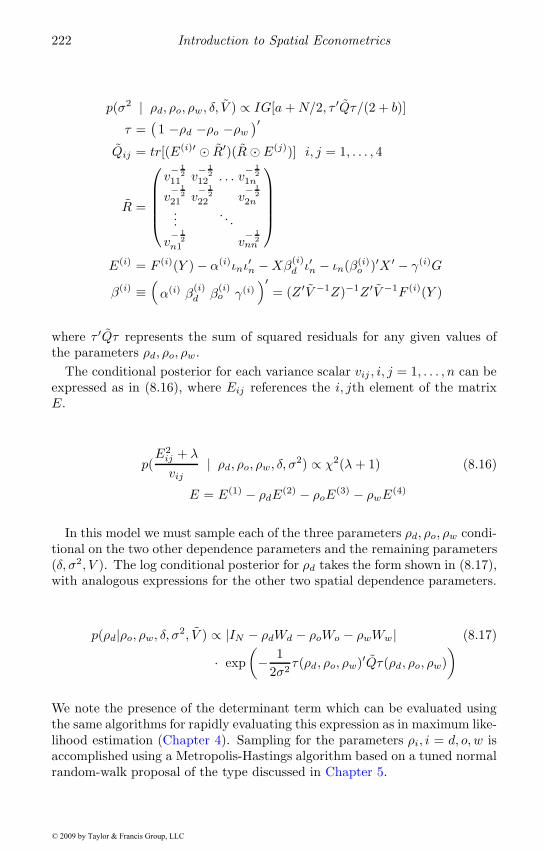
222 Introduction to Spatial Econometrics
p(σ2 | ρd, ρo, ρw, δ, V ) ∝ IG[a+N/2, τ ′Qτ/(2 + b)]
τ =(1 −ρd −ρo −ρw
)′Qij = tr[(E(i)′ � R′)(R � E(j))] i, j = 1, . . . , 4
R =
⎛⎜⎜⎜⎜⎝v− 1
211 v
− 12
12 . . . v− 1
21n
v− 1
221 v
− 12
22 v− 1
22n
.... . .
v− 1
2n1 v
− 12
nn
⎞⎟⎟⎟⎟⎠E(i) = F (i)(Y ) − α(i)ιnι
′n −Xβ
(i)d ι′n − ιn(β(i)
o )′X ′ − γ(i)G
β(i) ≡(α(i) β
(i)d β
(i)o γ(i)
)′= (Z ′V −1Z)−1Z ′V −1F (i)(Y )
where τ ′Qτ represents the sum of squared residuals for any given values ofthe parameters ρd, ρo, ρw.
The conditional posterior for each variance scalar vij , i, j = 1, . . . , n can beexpressed as in (8.16), where Eij references the i, jth element of the matrixE.
p(E2ij + λ
vij| ρd, ρo, ρw, δ, σ2) ∝ χ2(λ + 1) (8.16)
E = E(1) − ρdE(2) − ρoE
(3) − ρwE(4)
In this model we must sample each of the three parameters ρd, ρo, ρw condi-tional on the two other dependence parameters and the remaining parameters(δ, σ2, V ). The log conditional posterior for ρd takes the form shown in (8.17),with analogous expressions for the other two spatial dependence parameters.
p(ρd|ρo, ρw, δ, σ2, V ) ∝ |IN − ρdWd − ρoWo − ρwWw | (8.17)
· exp(− 1
2σ2τ(ρd, ρo, ρw)′Qτ(ρd, ρo, ρw)
)
We note the presence of the determinant term which can be evaluated usingthe same algorithms for rapidly evaluating this expression as in maximum like-lihood estimation (Chapter 4). Sampling for the parameters ρi, i = d, o, w isaccomplished using a Metropolis-Hastings algorithm based on a tuned normalrandom-walk proposal of the type discussed in Chapter 5.
© 2009 by Taylor & Francis Group, LLC
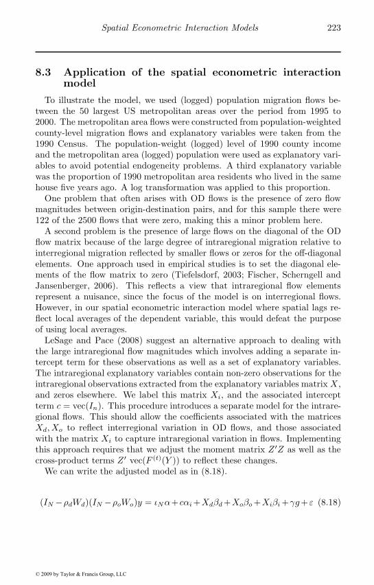
Spatial Econometric Interaction Models 223
8.3 Application of the spatial econometric interactionmodel
To illustrate the model, we used (logged) population migration flows be-tween the 50 largest US metropolitan areas over the period from 1995 to2000. The metropolitan area flows were constructed from population-weightedcounty-level migration flows and explanatory variables were taken from the1990 Census. The population-weight (logged) level of 1990 county incomeand the metropolitan area (logged) population were used as explanatory vari-ables to avoid potential endogeneity problems. A third explanatory variablewas the proportion of 1990 metropolitan area residents who lived in the samehouse five years ago. A log transformation was applied to this proportion.
One problem that often arises with OD flows is the presence of zero flowmagnitudes between origin-destination pairs, and for this sample there were122 of the 2500 flows that were zero, making this a minor problem here.
A second problem is the presence of large flows on the diagonal of the ODflow matrix because of the large degree of intraregional migration relative tointerregional migration reflected by smaller flows or zeros for the off-diagonalelements. One approach used in empirical studies is to set the diagonal ele-ments of the flow matrix to zero (Tiefelsdorf, 2003; Fischer, Scherngell andJansenberger, 2006). This reflects a view that intraregional flow elementsrepresent a nuisance, since the focus of the model is on interregional flows.However, in our spatial econometric interaction model where spatial lags re-flect local averages of the dependent variable, this would defeat the purposeof using local averages.
LeSage and Pace (2008) suggest an alternative approach to dealing withthe large intraregional flow magnitudes which involves adding a separate in-tercept term for these observations as well as a set of explanatory variables.The intraregional explanatory variables contain non-zero observations for theintraregional observations extracted from the explanatory variables matrix X ,and zeros elsewhere. We label this matrix Xi, and the associated interceptterm c = vec(In). This procedure introduces a separate model for the intrare-gional flows. This should allow the coefficients associated with the matricesXd, Xo to reflect interregional variation in OD flows, and those associatedwith the matrix Xi to capture intraregional variation in flows. Implementingthis approach requires that we adjust the moment matrix Z ′Z as well as thecross-product terms Z ′ vec(F (t)(Y )) to reflect these changes.
We can write the adjusted model as in (8.18).
(IN −ρdWd)(IN −ρoWo)y = ιNα+cαi+Xdβd+Xoβo+Xiβi+γg+ε (8.18)
© 2009 by Taylor & Francis Group, LLC
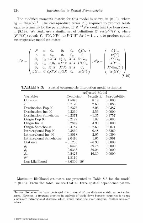
224 Introduction to Spatial Econometrics
The modified moments matrix for this model is shown in (8.19), wheredg = diag(G).3 The cross-product terms Z ′y required to produce least-squares estimates for the parameters, (Z ′Z)−1Z ′y would take the form shownin (8.19). We could use a similar set of definitions Z ′ vec(F (t)(Y )), where(F (t)(Y )) equals Y , WY , YW ′, or WYW ′ for t = 1, . . . , 4 to produce spatialautoregressive model estimates.
Z ′Z =
⎛⎜⎜⎜⎜⎜⎜⎝N n 0k 0k 0k ι′nGιnn n 0k 0k 0k 00k 0k nX ′X 0′k0k X ′X X ′Gιn0k 0k 0′k0k nX ′X X ′X X ′G′ιn0k 0k X ′X X ′X X ′X 0′k
ι′nG′ιn 0 ι′nG
′X ι′nGX 0k tr(G2)
⎞⎟⎟⎟⎟⎟⎟⎠ , Z ′y =
⎛⎜⎜⎜⎜⎜⎜⎝ι′nY ιntr(Y )X ′Y ιnX ′Y ′ιn
X ′diag(Y )tr(GY )
⎞⎟⎟⎟⎟⎟⎟⎠(8.19)
TABLE 8.3: Spatial econometric interaction model estimatesAdjusted Model
Variables Coefficient t-statistic t-probabilityConstant 1.5073 8.19 0.0000c 0.7170 2.63 0.0086Destination Pop 90 0.2376 2.06 0.0387Destination Inc 90 0.3269 5.56 0.0000Destination Samehouse −0.2371 −1.35 0.1757Origin Pop 90 0.2129 1.82 0.0683Origin Inc 90 0.2842 4.90 0.0000Origin Samehouse −0.4787 −2.69 0.0071Intraregional Pop 90 0.3869 0.48 0.6269Intraregional Inc 90 0.8018 2.05 0.0399Intraregional Samehouse 2.0410 1.65 0.0991Distance −0.1255 −6.30 0.0000ρd 0.6428 39.78 0.0000ρo 0.6358 39.25 0.0000ρw −0.5427 −16.39 0.0000σ2 1.8119Log-Likelihood −3.6309 ·103
Maximum likelihood estimates are presented in Table 8.3 for the modelin (8.18). From the table, we see that all three spatial dependence param-
3In our discussion we have portrayed the diagonal of the distance matrix as containingzeros. However, a frequent practice in analysis of trade flows between countries is to usea non-zero intraregional distance which would make the main diagonal contain non-zerovalues.
© 2009 by Taylor & Francis Group, LLC
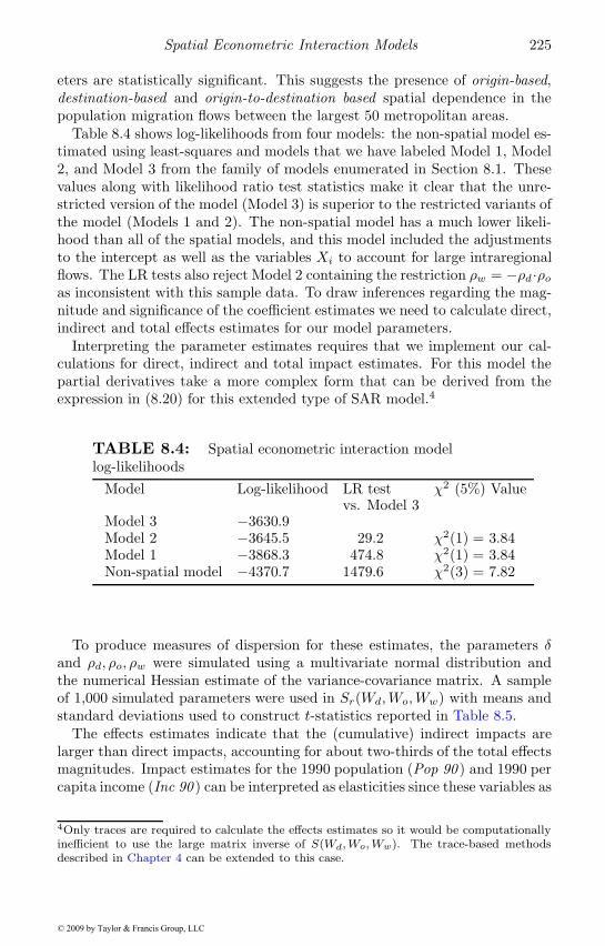
Spatial Econometric Interaction Models 225
eters are statistically significant. This suggests the presence of origin-based,destination-based and origin-to-destination based spatial dependence in thepopulation migration flows between the largest 50 metropolitan areas.
Table 8.4 shows log-likelihoods from four models: the non-spatial model es-timated using least-squares and models that we have labeled Model 1, Model2, and Model 3 from the family of models enumerated in Section 8.1. Thesevalues along with likelihood ratio test statistics make it clear that the unre-stricted version of the model (Model 3) is superior to the restricted variants ofthe model (Models 1 and 2). The non-spatial model has a much lower likeli-hood than all of the spatial models, and this model included the adjustmentsto the intercept as well as the variables Xi to account for large intraregionalflows. The LR tests also reject Model 2 containing the restriction ρw = −ρd ·ρoas inconsistent with this sample data. To draw inferences regarding the mag-nitude and significance of the coefficient estimates we need to calculate direct,indirect and total effects estimates for our model parameters.
Interpreting the parameter estimates requires that we implement our cal-culations for direct, indirect and total impact estimates. For this model thepartial derivatives take a more complex form that can be derived from theexpression in (8.20) for this extended type of SAR model.4
TABLE 8.4: Spatial econometric interaction modellog-likelihoods
Model Log-likelihood LR test χ2 (5%) Valuevs. Model 3
Model 3 −3630.9Model 2 −3645.5 29.2 χ2(1) = 3.84Model 1 −3868.3 474.8 χ2(1) = 3.84Non-spatial model −4370.7 1479.6 χ2(3) = 7.82
To produce measures of dispersion for these estimates, the parameters δand ρd, ρo, ρw were simulated using a multivariate normal distribution andthe numerical Hessian estimate of the variance-covariance matrix. A sampleof 1,000 simulated parameters were used in Sr(Wd,Wo,Ww) with means andstandard deviations used to construct t-statistics reported in Table 8.5.
The effects estimates indicate that the (cumulative) indirect impacts arelarger than direct impacts, accounting for about two-thirds of the total effectsmagnitudes. Impact estimates for the 1990 population (Pop 90 ) and 1990 percapita income (Inc 90 ) can be interpreted as elasticities since these variables as
4Only traces are required to calculate the effects estimates so it would be computationallyinefficient to use the large matrix inverse of S(Wd, Wo, Ww). The trace-based methodsdescribed in Chapter 4 can be extended to this case.
© 2009 by Taylor & Francis Group, LLC
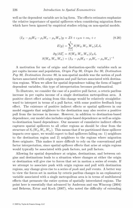
226 Introduction to Spatial Econometrics
well as the dependent variable are in log form. The effects estimates emphasizethe relative importance of spatial spillovers when considering migration flowswhich have been ignored by empirical studies relying on non-spatial models.
(IN − ρdWd − ρoWo − ρwWw)y = Zδ + ιNα+ cαi + ε (8.20)
E(y) =k∑r=1
S(Wd,Wo,Ww)Zrδr
∂y/∂Z ′r = S(Wd,Wo,Ww)IN δr
S(Wd,Wo,Ww) = (IN − ρdWd − ρoWo − ρwWw)−1
A motivation for use of origin- and destination-specific variables such asper capita income and population, Origin Pop 90, Origin Inc 90, DestinationPop 90, Destination Income 90, in non-spatial models was the notion of pushfactors associated with origin regions and pull factors associated with destina-tion regions. When we allow for spatial dependence taking the form of laggeddependent variables, this type of interpretation becomes problematical.
To illustrate, we consider the case of a positive pull factor, a ceteris paribusincrease in per capita income of a single destination metropolitan area. Apositive direct effect arising from this change would be relatively straightfor-ward to interpret in terms of a pull factor, with some positive feedback loopeffect. The existence of positive indirect effects or spatial spillovers in ourmodel suggests that neighbors to the destination may also receive a positivepull from the increase in income. However, in addition to destination-baseddependence, our model also includes origin-based dependence as well as origin-to-destination based dependence. Our measure of cumulative indirect effectscaptures spatial spillovers to all other regions as should be clear from thestructure of Sr(Wd,Wo,Ww). This means that if we partitioned these spilloverimpacts over space, we would expect to find spillovers falling on: 1) neighborsto the destination region and 2) neighbors to the regions where migrationflows originate. This makes it more difficult to rely on the conventional pullfactor interpretation, since spatial spillover effects that arise at origin regionswould typically be associated with push factors, not pull factors.
Allowing for spatial dependence at origins, destinations, and between ori-gins and destinations leads to a situation where changes at either the originor destination will give rise to forces that set in motion a series of events. Ifwe attempt to associate push with origin regions and pull with destinationregions, any change gives rise to a series of push and pull events. A better wayto view the forces set in motion by ceteris paribus changes in an explanatoryvariable associated with a single metropolitan area is in terms of multilateraleffects that permeate the entire system of spatially interrelated regions. Thepoint here is essentially that advanced by Anderson and van Wincoop (2004)and Behrens, Ertur and Koch (2007), who noted the difficulty of extending
© 2009 by Taylor & Francis Group, LLC
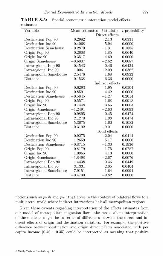
Spatial Econometric Interaction Models 227
TABLE 8.5: Spatial econometric interaction model effectsestimates
Variables Mean estimates t-statistic t-probabilityDirect effects
Destination Pop 90 0.2982 2.13 0.0331Destination Inc 90 0.4068 5.94 0.0000Destination Samehouse −0.2870 −1.31 0.1885Origin Pop 90 0.2608 1.85 0.0640Origin Inc 90 0.3517 4.69 0.0000Origin Samehouse −0.6007 −2.62 0.0087Intraregional Pop 90 0.4543 0.46 0.6434Intraregional Inc 90 1.0061 2.09 0.0362Intraregional Samehouse 2.5476 1.68 0.0922Distance −0.1538 −6.36 0.0000
Indirect effectsDestination Pop 90 0.6293 1.95 0.0504Destination Inc 90 0.8591 4.42 0.0000Destination Samehouse −0.5845 −1.27 0.2014Origin Pop 90 0.5571 1.68 0.0918Origin Inc 90 0.7448 3.65 0.0003Origin Samehouse −1.2491 −2.60 0.0093Intraregional Pop 90 0.9895 0.45 0.6474Intraregional Inc 90 2.1270 1.98 0.0474Intraregional Samehouse 5.3675 1.60 0.1082Distance −0.3192 −9.01 0.0000
Total effectsDestination Pop 90 0.9275 2.04 0.0414Destination Inc 90 1.2659 5.17 0.0000Destination Samehouse −0.8715 −1.30 0.1936Origin Pop 90 0.8179 1.75 0.0787Origin Inc 90 1.0965 4.13 0.0000Origin Samehouse −1.8498 −2.67 0.0076Intraregional Pop 90 1.4438 0.46 0.6449Intraregional Inc 90 3.1331 2.05 0.0404Intraregional Samehouse 7.9151 1.64 0.0994Distance −0.4730 −9.82 0.0000
notions such as push and pull that arose in the context of bilateral flows to amultilateral world where indirect interactions link all metropolitan regions.
Given these caveats regarding interpretation of the effects estimates fromour model of metropolitan migration flows, the most salient interpretationof these effects might be in terms of differences between the direct and in-direct effects of origin and destination variables. For example, the positivedifference between destination and origin direct effects associated with percapita income (0.40 − 0.35) could be interpreted as meaning that positive
© 2009 by Taylor & Francis Group, LLC
228 Introduction to Spatial Econometrics
(1990) income gaps between metropolitan areas gave rise to increased migra-tion flows to metropolitan areas having relatively higher per capita incomes.The positive difference between indirect effects associated with (1990) percapita income of destination and origin metropolitan areas (0.86− 0.74) sug-gests that (1990) income gaps between metropolitan areas led to spillovers thatincreased migration flows to all other regions. Given what we know about thespatial structure of indirect or spatial spillover effects, these increased mi-gration flows most likely impacted regions that were neighbors to origin anddestination metropolitan areas exhibiting large relative income gaps.
There is a similar pattern of positive differences between the direct ef-fects associated with the destination and origin (1990) population variable(0.29 − 0.26). This suggests positive migration flows arose as a result of(1990) population size differences that had a positive direct impact on des-tination metropolitan areas. The positive difference between indirect effects(0.63−0.55) suggests that (1990) population gaps between metropolitan areasled to spatial spillover effects that gave rise to higher levels of migration flowsto all other regions, in a fashion similar to gaps in (1990) per capita income.
The origin and destination Samehouse variables exhibit negative direct andindirect effects, suggesting lower (1995-2000) migration flows for metropolitanareas where more people lived in the same house in 1990 as in 1985. This alsoresulted in negative spatial spillovers, meaning lower levels of migration flowfor other metropolitan regions as well.
If our interest centered on interregional migration flows, we might viewthe intraregional variables as controls and the associated effects estimates asnuisance parameters. However, the positive direct effect elasticity of 1 andindirect effect elasticity of 2.12 leads to a total effect greater than 3. This sug-gests the direct or own-region effect of (1990) per capita income on migrationflows was positive as was the indirect effect. Intraregional (1990) populationalso had positive but not significant direct, indirect and total effects. Thetotal effect of the intraregional Samehouse variable is large and positive, butsignificant only at the 90 percent level.
The distance estimate has a total effect of −0.48 which is much largerthan one would infer from the model coefficients reported in Table 8.3. Themodel coefficient is of course close to the direct effect estimate in Table 8.5, atypical result noted earlier in our discussion regarding interpretation of impactestimates from these models.
8.4 Extending the spatial econometric interaction model
There are a number of problems that are encountered in empirical modelingof OD flows. The next sections describe three extensions of these models that
© 2009 by Taylor & Francis Group, LLC
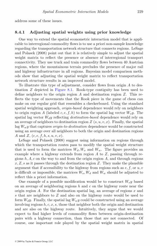
Spatial Econometric Interaction Models 229
address some of these issues.
8.4.1 Adjusting spatial weights using prior knowledge
One way to extend the spatial econometric interaction model that is appli-cable to interregional commodity flows is to use a priori non-sample knowledgeregarding the transportation network structure that connects regions. LeSageand Polasek (2008) point out that it is relatively simple to adjust the spatialweight matrix to reflect the presence or absence of interregional transportconnectivity. They use truck and train commodity flows between 40 Austrianregions, where the mountainous terrain precludes the presence of major railand highway infrastructure in all regions. Bayesian model comparison meth-ods show that adjusting the spatial weight matrix to reflect transportationnetwork structure results in an improved model.
To illustrate this type of adjustment, consider flows from origin A to des-tination Z depicted in Figure 8.1. Rook-type contiguity has been used todefine neighbors to the origin region A and destination region Z. This re-flects the type of movements that the Rook piece in the game of chess canmake on our regular grid that resembles a checkerboard. Using the standardspatial weighting approach, origin-based dependence would rely on neighborsto origin region A (labeled c, e, f, h) to form the spatial lag vector Woy. Thespatial lag vector Wdy reflecting destination-based dependence would rely onan average of neighbors to destination region Z (s, u, v, x). Finally, the spatiallag Wwy that captures origin-to-destination dependence would be constructedusing an average over all neighbors to both the origin and destination regionsA and Z, (c, e, f, h, s, u, v, x).
LeSage and Polasek (2008) suggest using information on regions throughwhich the transportation routes pass to modify the spatial weight structurethat is used to form the matrices Wd,Wo and Ww. The figure provides anexample where a highway extends from region A to Z, passing through re-gions h,A, c on the way to and from the origin region A, and through regionsx, Z, s as it passes through the destination region Z. They make the plausibleargument that if accessibility to the highway from regions such as e, f, or u, vis difficult or impossible, the matrices Wo,Wd and Ww should be adjusted toreflect this a priori information.
One example of a possible modification would be to construct Woy basedon an average of neighboring regions h and c on the highway route near theorigin region A. For the destination spatial lag, an average of regions x ands that are neighbors to Z and also on the highway route would be used toform Wdy. Finally, the spatial lag Wwy could be constructed using an averageinvolving regions h, c, x, s, those that neighbor both the origin and destinationand are also on the highway route. Intuitively, they argue that we wouldexpect to find higher levels of commodity flows between origin-destinationpairs with a highway connection, than those that are not connected. Ofcourse, one important role played by the spatial weight matrix in spatial
© 2009 by Taylor & Francis Group, LLC
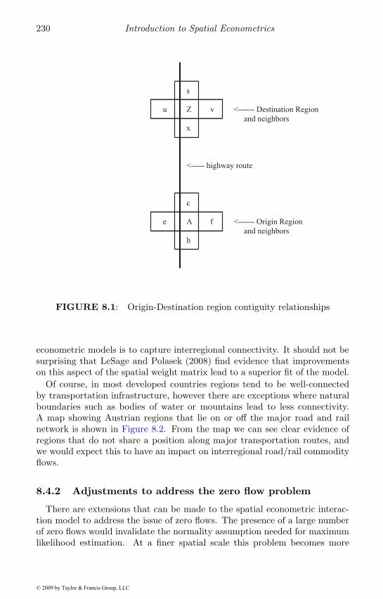
230 Introduction to Spatial Econometrics
e
h
A
c
f
u
x
Z
s
v
<----- highway route
<------ Origin Region
and neighbors
<------ Destination Region
and neighbors
FIGURE 8.1: Origin-Destination region contiguity relationships
econometric models is to capture interregional connectivity. It should not besurprising that LeSage and Polasek (2008) find evidence that improvementson this aspect of the spatial weight matrix lead to a superior fit of the model.
Of course, in most developed countries regions tend to be well-connectedby transportation infrastructure, however there are exceptions where naturalboundaries such as bodies of water or mountains lead to less connectivity.A map showing Austrian regions that lie on or off the major road and railnetwork is shown in Figure 8.2. From the map we can see clear evidence ofregions that do not share a position along major transportation routes, andwe would expect this to have an impact on interregional road/rail commodityflows.
8.4.2 Adjustments to address the zero flow problem
There are extensions that can be made to the spatial econometric interac-tion model to address the issue of zero flows. The presence of a large numberof zero flows would invalidate the normality assumption needed for maximumlikelihood estimation. At a finer spatial scale this problem becomes more
© 2009 by Taylor & Francis Group, LLC
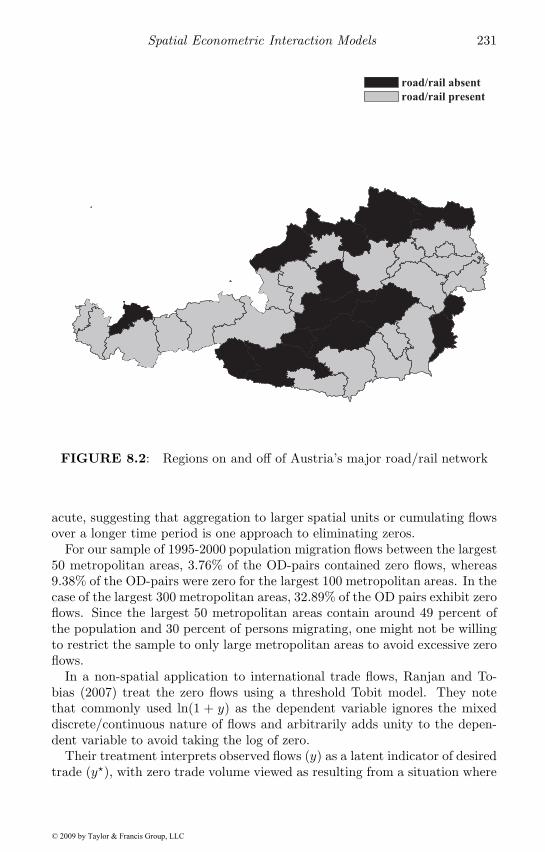
Spatial Econometric Interaction Models 231
road/rail absent
road/rail present
FIGURE 8.2: Regions on and off of Austria’s major road/rail network
acute, suggesting that aggregation to larger spatial units or cumulating flowsover a longer time period is one approach to eliminating zeros.
For our sample of 1995-2000 population migration flows between the largest50 metropolitan areas, 3.76% of the OD-pairs contained zero flows, whereas9.38% of the OD-pairs were zero for the largest 100 metropolitan areas. In thecase of the largest 300 metropolitan areas, 32.89% of the OD pairs exhibit zeroflows. Since the largest 50 metropolitan areas contain around 49 percent ofthe population and 30 percent of persons migrating, one might not be willingto restrict the sample to only large metropolitan areas to avoid excessive zeroflows.
In a non-spatial application to international trade flows, Ranjan and To-bias (2007) treat the zero flows using a threshold Tobit model. They notethat commonly used ln(1 + y) as the dependent variable ignores the mixeddiscrete/continuous nature of flows and arbitrarily adds unity to the depen-dent variable to avoid taking the log of zero.
Their treatment interprets observed flows (y) as a latent indicator of desiredtrade (y�), with zero trade volume viewed as resulting from a situation where
© 2009 by Taylor & Francis Group, LLC
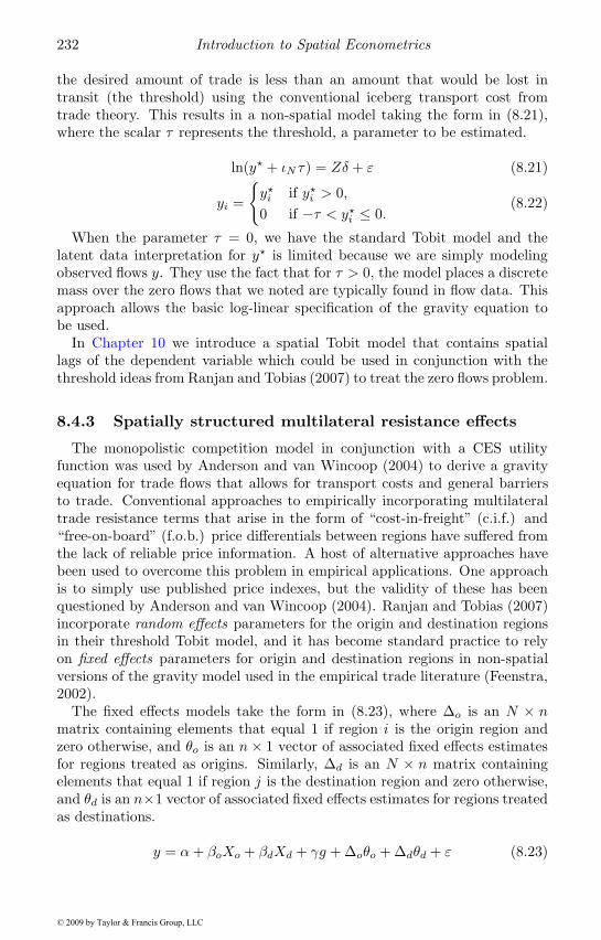
232 Introduction to Spatial Econometrics
the desired amount of trade is less than an amount that would be lost intransit (the threshold) using the conventional iceberg transport cost fromtrade theory. This results in a non-spatial model taking the form in (8.21),where the scalar τ represents the threshold, a parameter to be estimated.
ln(y� + ιN τ) = Zδ + ε (8.21)
yi =
{y�i if y�i > 0,0 if −τ < y�i ≤ 0.
(8.22)
When the parameter τ = 0, we have the standard Tobit model and thelatent data interpretation for y� is limited because we are simply modelingobserved flows y. They use the fact that for τ > 0, the model places a discretemass over the zero flows that we noted are typically found in flow data. Thisapproach allows the basic log-linear specification of the gravity equation tobe used.
In Chapter 10 we introduce a spatial Tobit model that contains spatiallags of the dependent variable which could be used in conjunction with thethreshold ideas from Ranjan and Tobias (2007) to treat the zero flows problem.
8.4.3 Spatially structured multilateral resistance effects
The monopolistic competition model in conjunction with a CES utilityfunction was used by Anderson and van Wincoop (2004) to derive a gravityequation for trade flows that allows for transport costs and general barriersto trade. Conventional approaches to empirically incorporating multilateraltrade resistance terms that arise in the form of “cost-in-freight” (c.i.f.) and“free-on-board” (f.o.b.) price differentials between regions have suffered fromthe lack of reliable price information. A host of alternative approaches havebeen used to overcome this problem in empirical applications. One approachis to simply use published price indexes, but the validity of these has beenquestioned by Anderson and van Wincoop (2004). Ranjan and Tobias (2007)incorporate random effects parameters for the origin and destination regionsin their threshold Tobit model, and it has become standard practice to relyon fixed effects parameters for origin and destination regions in non-spatialversions of the gravity model used in the empirical trade literature (Feenstra,2002).
The fixed effects models take the form in (8.23), where Δo is an N × nmatrix containing elements that equal 1 if region i is the origin region andzero otherwise, and θo is an n× 1 vector of associated fixed effects estimatesfor regions treated as origins. Similarly, Δd is an N × n matrix containingelements that equal 1 if region j is the destination region and zero otherwise,and θd is an n×1 vector of associated fixed effects estimates for regions treatedas destinations.
y = α+ βoXo + βdXd + γg + Δoθo + Δdθd + ε (8.23)
© 2009 by Taylor & Francis Group, LLC
Spatial Econometric Interaction Models 233
This approach interprets the parameters in the vector θo as latent “prices”or multilateral resistance indices for the n regions viewed as origins and sim-ilarly for the parameters θd for the destinations.
Spatially structured random effects seem more plausible since this approachintroduces latent effects parameters that are structured to follow a spatialautoregressive process. We provided one motivation for this in Section 2.3based on spatial heterogeneity. This type of model can be viewed as imposinga “stochastic restriction” on the origin-destination effects parameters so thatmultilateral resistance is similar for neighboring regions. This is motivated bythe notion that latent or unobservable barriers to regional trade (which areusually motivated theoretically as price differential effects) should be similarfor regions that are located nearby. As in the case of fixed effects, a set of2n individual effects parameters is estimated using the sample of N OD flowobservations. This approach was introduced by LeSage and Llano (2007) tomodel commodity flows between Spanish regions. The model takes the formin (8.24).
y = Zδ + Δdθd + Δoθo + ε (8.24)θd = ρdWθd + ud
θo = ρoWθo + u0
ud ∼ N(0, σ2dIn)
uo ∼ N(0, σ2oIn)
Given an origin-centric orientation of the flow matrix (columns as originsand rows as destinations), the matrices Δd = In ⊗ ιn and Δo = ιn ⊗ Inproduce N by n matrices. It should be noted that estimates for these twosets of random effects parameters are identified, since a set of n sample dataobservations are aggregated through the matrices Δd and Δo to produce eachestimate in θd, θo.
The spatial autoregressive structure placed on the origin and destinationeffects reflects an implied prior for the spatial effects vector θd conditional onρd, σ
2d and for θo conditional on ρo, σ2
o shown in (8.25) and (8.26).
π(θd|ρd, σ2d) ∼ (σ2
d)n/2|Bd|exp
(− 1
2σ2d
θ′dB′dBdθd
)(8.25)
π(θo|ρo, σ2o) ∼ (σ2
o)n/2|Bo|exp
(− 1
2σ2o
θ′oB′oBoθo
)(8.26)
Bd = In − ρdW
Bo = In − ρoW
Estimation of the spatially structured origin effects vector θo requires intro-duction of two additional parameters (ρo, σ2
o) to the model. One of these con-trols the strength of spatial dependence between regions (treated as origins)
© 2009 by Taylor & Francis Group, LLC
234 Introduction to Spatial Econometrics
and the other controls the variance/uncertainty of the prior spatial structure.Given these two scalar parameters along with the spatial structure, the n ori-gin effects parameters are completely determined. One could view the spatialconnectivity matrix W as introducing additional exogenous information thataugments the sample data information. In contrast, the conventional fixedorigin effects approach introduces n additional parameters to be estimatedwithout (materially) augmenting the sample data information.
Another point about the spatially structured prior is that if the scalar spa-tial dependence parameters (ρo, ρd) are not significantly different from zero,the spatial structure of the effects vectors disappears, leaving us with normallydistributed random effects parameters for the origins and destinations similarto the model of Ranjan and Tobias (2007). LeSage and Llano (2007) pro-vide details regarding Bayesian MCMC estimation of this hierarchical linearmodel.
8.4.4 Flows as a rare event
For some OD flow matrices that contain an extremely large proportion of ze-ros, the argument for sample truncation seems questionable. LeSage, Fischerand Scherngell (2007) extend the model in (8.14) using results from Fruhwirth-Schnatter and Wagner (2006). In their examination they treat interregionalpatent citations from a sample of European Union regions as representingknowledge flows. Counts of patents originating in region i that were cited byregions j = 1, . . . , n are used to form an OD knowledge flow matrix. Sincecross-region patent citations are both counts and rare events, a Poisson distri-bution seems much more plausible than the normal distribution required formaximum likelihood estimation of the spatial econometric interaction model.
Fruhwirth-Schnatter and Wagner (2006) argue that (non-spatial) Poissonregression models (including those with random-effects) can be treated asa partially Gaussian regression model by conditioning on two strategicallychosen sequences of artificially missing data. Chapter 10 provides more de-tails regarding Bayesian treatment of binary 0,1 observations as indicators oflatent unobserved utility, an idea originated by Albert and Chib (1993). Af-ter conditioning on both of these latent sequences, Fruhwirth-Schnatter andWagner (2006) show that the resulting model can be sampled using Gibbssampling of all regression parameters and the latent sequences. This requiresrandom draws from only known distributions such as multivariate normal, in-verse Gamma, exponential, and a discrete distribution with a limited numberof categories, which eliminates the need for use of Metropolis-Hastings stepsduring sampling.
There is a large literature on Bayesian hierarchical spatial models (Baner-jee, Carlin and Gelfand, 2004; Cressie, 1995), but this work cannot be appliedto the case of non-linear Poisson regression models in a straightforward fash-ion. The tremendous advantage of the approach introduced by Fruhwirth-Schnatter and Wagner (2006) is that this large suite of existing hierarchical
© 2009 by Taylor & Francis Group, LLC
Spatial Econometric Interaction Models 235
linear spatial models can be directly applied after augmenting the existingsampling scheme with the two latent sequences. The addition of these twolatent variable vectors does not affect the conditional distributions of existinghierarchical models, so existing algorithms and code can be used.
The one drawback to the approach is that one must sample two sets oflatent parameters equal to yij+1, where yij denotes the count for observationi. Specifically, if we have a sample i = 1, . . . , n, and half of these observationsexhibit magnitudes of yij = 0, while the other half take on non-zero countvalues of yij = 10, then we must sample two vectors of latent parameters equalto 11(n/2) + (n/2), where the 11(n/2) latent parameters are associated withthe non-zero counts where yij +1 = 11, and the n/2 parameters with the zerocounts where yij+1 = 1. For the sample of n = 188 regions in LeSage, Fischerand Scherngell (2007), there were 23,718 zero values and
∑ji yij+1 = 109, 817,
for a total of 133,535 latent observations needed to sample each of the twolatent variable vectors.
For the spatially structured random effects model from (8.14), let y =(y1, . . . , yN ) denote our sample of N = n2 counts for the OD pairs of regions.The assumption regarding yi is that yi|λi follows a Poisson, P(λi) distribution,where λi depends on (standardized) covariates zi with associated parametervector γ as well as n vectors of latent spatial effects parameters. This modelcan be expressed as:
yi|λi ∼ P(λi), (8.27)λi = exp(ziγ + δdiθd + δoiθo)
where δdi represents the ith row from the matrix Δd that identifies region ias a destination region and δoi identifies origin regions using rows from thematrix Δo.
Fruhwirth-Schnatter and Wagner (2006) note that the posterior densitytakes the form in (8.28), where V are parameters and ψ are the latent unob-servables on which we are conditioning.
p(V|ψ, y) ∝ p(y|V)p(V|ψ) (8.28)
p(y|V) =N∏i=1
exp(ziδ)yi
yi!exp(−exp(ziδ))
The use of a normal distribution for the random effects in place of the con-jugate gamma distribution results in a posterior density that does not belongto a density from a known distribution family. The contribution of Fruhwirth-Schnatter and Wagner (2006) was to note that introduction of two sequencesof artificially missing data (treated using data augmentation) can lead to asequence of conditional posteriors for the parameters V that take the sameform as those that would arise if our model was a normal linear model. One
© 2009 by Taylor & Francis Group, LLC
236 Introduction to Spatial Econometrics
of the two sequences of artificially missing data eliminates the non-linearity ofthe Poisson model using ideas regarding unobserved inter-arrival times froma Poisson process. After eliminating the non-linearity, a linear regressionmodel results, where the non-normal errors follow a log exponential distri-bution having a mean of unity. The second sequence of missing data is acomponent indicator associated with a normal mixture approximation to thelog exponential distribution that is used to eliminate the non-normality.
8.5 Chapter summary
Standard spatial regression models rely on spatial autoregressive constructsthat use spatial weight structures to specify dependence among n regions.Ways of parsimoniously modeling the connectivity among the sample of N =n2 origin-destination (OD) pairs that arise in a closed system of interregionalflows has remained a stumbling block. We demonstrated that the algebraof Kronecker products can be used to produce spatial weight structures thatmodel dependence among the N OD pairs in a fashion consistent with stan-dard spatial autoregressive processes. This allows us to extend spatial regres-sion models that have served as the workhorse in applied spatial econometricanalysis to model OD flows. The resulting models reflect a spatial filter fororigin- and destination-based dependence, as well as an interaction term thatwe label origin-to-destination based dependence.
Important computational issues arise when working with OD flows sincethe sample is of dimension N = n2, where n is the number of regions beingmodeled. We provide a moment-matrix approach that can be used for bothmaximum likelihood and Bayesian estimation of the models set forth here.The computational time and memory required by our approach to estimationdoes not depend on the sample size n, making it applicable to large problems.
© 2009 by Taylor & Francis Group, LLC
Chapter 9
Matrix Exponential Spatial Models
This chapter discusses a matrix exponential spatial specification (MESS) in-troduced by LeSage and Pace (2007). As discussed in Section 7.6, one canview MESS as arising from a spatiotemporal process with exponential decayof influence from previous periods. The matrix exponential can provide analternative to the spatial autoregressive process as a basis for building spatialregression models. It essentially replaces the geometric decay over space as-sociated with the spatial autoregressive process with exponential decay overspace.
This alternative has a computational advantage over conventional spatialautoregressive based regression models since it eliminates the need to calculatethe log-determinant when producing maximum likelihood and Bayesian modelestimates. There are also theoretical advantages associated with this type ofspatial specification.
Section 9.1 presents the matrix exponential spatial specification, which welabel the MESS model. This specification replaces the spatial autoregressiveprocess with a matrix exponential spatial transformation. In Section 9.2 weintroduce the idea of modeling spatial error variance-covariance matrices asa matrix exponential and show how this can be applied to produce a spa-tial regression specification. We describe a number of connections betweenvarious traditional spatial error model specifications that can be establishedusing the matrix exponential spatial specification. A Bayesian version of themodel is introduced in Section 9.3, and the basic MESS model is extended inSection 9.4 to include a parameterized spatial weight structure. Estimationof this extended model using MCMC is discussed and illustrated. Section 9.5extends the MESS model to implement spatial fractional differencing.
9.1 The MESS model
In Section 9.1.1, we present a unique interior optimal spatial transforma-tion of the dependent variable that leads to the MESS model. Section 9.1.2discusses maximum likelihood estimation using this model, and Section 9.1.3provides details on a closed form solution for this model using the approach
237© 2009 by Taylor & Francis Group, LLC
238 Introduction to Spatial Econometrics
discussed in Chapter 4.
9.1.1 The matrix exponential
Consider estimation of models where the dependent variable y undergoes alinear transformation Sy as in (9.1).
Sy = Xβ + ε (9.1)
The vector y contains the n observations on the dependent variable, Xrepresents the n × k matrix of observations on the independent variables, Sis a positive definite n × n matrix, and the n-element vector ε is distributedN(0, σ2In). Note that a conventional spatial autoregressive model can bewritten by setting S = (In − ρW ) in (9.1). The concentrated log-likelihoodfor the model in (9.1) is shown in (9.2), where β and σ2 have been concentratedout of the model.
L = κ+ ln|S| − (n/2)ln(y′S′MSy) (9.2)
The term κ represents a scalar constant and both M = In − H and H =X(X ′X)−1X ′ are idempotent matrices. The term |S| is the Jacobian of thetransformation from y to Sy. Without the Jacobian term, S containing allzeros would lead to a perfect, albeit pathological fit as noted in Chapter 4.The Jacobian term penalizes attempts to use singular or near singular trans-formations to artificially increase the regression fit.
The matrix exponential defined in (9.3) can be used as a model for S, whereW represents an n× n non-negative matrix with zeros on the diagonal and αrepresents a scalar real parameter.
S = eαW =∞∑i=0
αiW i
i!(9.3)
Of course, W is a spatial weight matrix, where Wij > 0 indicates that ob-servation j is a neighbor of observation i. As usual, Wii = 0 to preclude anobservation from directly predicting itself. Also, (W 2)ij > 0 indicates thatobservation j is a neighbor to a neighbor of observation i. Similar relationshold for higher powers of W which identify higher-order neighbors. Thus thematrix exponential S, associated with matrix W , imposes a decay of influencefor higher-order neighboring relationships. The MESS specification replacesthe conventional geometric decay of influence from higher-order neighboringrelationships implied by the spatial autoregressive process with an exponentialpattern of decay in influence from higher-order neighboring relationships.
As in the case of conventional autoregressive processes, ifW is row-stochastic,S will be proportional to a row-stochastic matrix, since products of row-stochastic matrices are row-stochastic (i.e., by definition Wιn = ιn and there-fore W (Wιn) = ιn, and so on, where ιn denotes a vector of ones). Con-
© 2009 by Taylor & Francis Group, LLC
Matrix Exponential Spatial Models 239
sequently, S is a linear combination of row-stochastic matrices and thus isproportional to a row-stochastic matrix.
In a non-spatial setting, Chiu, Leonard, and Tsui (1996) proposed use ofthe matrix exponential and discussed several of its salient properties, some ofwhich are enumerated below:
1. S is positive definite,
2. any positive definite matrix is the matrix exponential of some matrix,
3. S−1 = e−αW ,
4. |eαW | = etr(αW ).
The last property greatly simplifies the MESS log-likelihood. Since tr(W ) =0 and by extension |eαW | = etr(αW ) = e0 = 1, the concentrated log-likelihoodtakes the form: L = κ − (n/2)ln(y′S′MSy). Therefore, maximizing the log-likelihood is equivalent to minimizing (y′S′MSy), the overall sum-of-squarederrors.
The MESS model in (9.1) can be extended in a fashion similar to the SDMmodel. Let U represent a matrix of observations on p non-constant indepen-dent variables and let q be an integer large enough so that X approximatelyspans SU , but small enough so that X cannot span y. The design matrix X(assuming full rank) could have the form (9.4).
X = [ιn U WU . . .W q−1U ] (9.4)
In this case, X approximately spans SU and thus the MESS model basedon (9.4) nests a spatial autoregression in the errors. Like the SDM model,this variant of the MESS model results in a situation where a set of linear re-strictions on the parameters associated with the columns of X could yield theerror autoregression. Hendry et al. (1984) advocates estimation of this type ofgeneral distributed lag model with subsequent imposition of restrictions thathas been labeled the general to specific approach to model specification.
9.1.2 Maximum likelihood estimation
If elements of the powers of W represent magnitudes that do not rise withthe power, the power series in (9.3) converges rapidly. Since row-stochastic,non-negative matrices W have a maximum of 1 in any row, the magnitude ofthe elements in the powers of W does not grow with powers of the matrix.Given a rapid decline in the coefficients of the power series, achieving a sat-isfactory progression towards convergence seems feasible with ten to twelveterms.
If the graph of W is strongly connected, meaning that a path exists betweenevery pair of observations, then
∑nr=1 ωrW
r will be dense (all non-zeros) forpositive ωr (Horn and Johnson, 1993, p. 361-362), leading to a dense S. In this
© 2009 by Taylor & Francis Group, LLC
240 Introduction to Spatial Econometrics
case, computing S separately would require prohibitive amounts of memoryand time for large n. Fortunately, we do not need to compute S separatelysince S always appears in conjunction with y. This allows computation of Syin O((q − 1)n2) operations for dense W by sequential left-multiplication of yby W to form n−element vectors, (i.e., Wy, W (Wy) = W 2y, and so on).
For sparse W the number of operations required to compute Sy declines toO((q−1)n �=0), where n �=0 denotes the number of non-zeros. For an m nearestneighbor spatial weight matrix that has m non-zero entries in each row, theoperation count associated with computing Sy would decline to O((q−1)mn).This results in an operation count for computing Sy in nearest neighbor spec-ifications of W that is linear in n.
9.1.3 A closed form solution for the parameters
Section 4.10 presented a means of finding closed-form solutions for manysingle dependence parameter models. In this section we show how to finda closed-form solution to MESS using this framework. To illustrate this ap-proach in detail, we define the n×q matrix Y comprised of powers of W timesy in (9.5).
Y = [y Wy W 2y . . .W q−1y] (9.5)
We define a diagonal matrix G1 containing some of the coefficients from thepower series as shown in (9.6).
G1 =
⎛⎜⎜⎜⎝1/0!
1/1!. . .
1/(q − 1)!
⎞⎟⎟⎟⎠ (9.6)
In addition, we define the q-element column vector v shown in (9.7) thatcontains powers of the scalar real parameter α, |α| <∞.
v(α) = [1 α α2 . . . αq−1]′ (9.7)
Using (9.5), (9.6) and (9.7), we can rewrite Sy as shown in (9.8).
Sy ≈ Y G1v(α) (9.8)
Premultiplying Sy by the least-squares idempotent matrix M yields the resid-uals e, allowing us to express the overall sum-of-squared errors as in (9.9),
e′e = v(α)′G1(Y ′M ′MY )G1v(α)= v(α)′G1(Y ′MY )G1v(α)= v(α)′Qv(α) (9.9)
© 2009 by Taylor & Francis Group, LLC
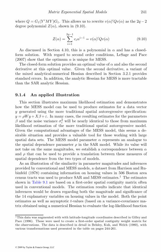
Matrix Exponential Spatial Models 241
where Q = G1(Y ′MY )G1. This allows us to rewrite v(α)′Qv(α) as the 2q− 2degree polynomial Z(α), shown in (9.10).
Z(α) =2q−1∑i=1
ciαi−1 = v(α)′Qv(α) (9.10)
As discussed in Section 4.10, this is a polynomial in α and has a closed-form solution. With regard to second order conditions, LeSage and Pace(2007) show that the optimum α is unique for MESS.
The closed-form solution provides an optimal value of α and also the secondderivative at this optimal value. Given the second derivative, a variant ofthe mixed analytical-numerical Hessian described in Section 3.2.1 providesstandard errors. In addition, the analytic Hessian for MESS is more tractablethan the SAR analytic Hessian.
9.1.4 An applied illustration
This section illustrates maximum likelihood estimation and demonstrateshow the MESS model can be used to produce estimates for a data vectory generated using the more traditional spatial autoregressive specification:y = ρWy+Xβ+ ε. In many cases, the resulting estimates for the parametersβ and the noise variance σ2
ε will be nearly identical to those from maximumlikelihood estimation of the more traditional spatial autoregressive model.Given the computational advantages of the MESS model, this seems a de-sirable situation and provides a valuable tool for those working with largespatial data sets. The MESS model parameter α represents an analogue tothe spatial dependence parameter ρ in the SAR model. While its value willnot take on the same magnitudes, we establish a correspondence between αand ρ that can be used to provide a translation between these measures ofspatial dependence from the two types of models.
As an illustration of the similarity in parameter magnitudes and inferencesprovided by conventional and MESS models, a dataset from Harrison and Ru-binfeld (1978) containing information on housing values in 506 Boston areacensus tracts was used to produce SAR and MESS estimates.1 The estimatesshown in Table 9.1 are based on a first-order spatial contiguity matrix oftenused in conventional models. The estimation results indicate that identicalinferences would be drawn regarding both the magnitude and significance ofthe 14 explanatory variables on housing values in the model. Both the pointestimates as well as asymptotic t-values (based on a variance-covariance ma-trix obtained using a numerical Hessian to evaluate the log-likelihood function
1This data was augmented with with latitude-longitude coordinates described in Gilley andPace (1996). These were used to create a first-order spatial contiguity weight matrix forthe observations. The data is described in detail in Belsley, Kuh, and Welch (1980), withvarious transformations used presented in the table on pages 244-261.
© 2009 by Taylor & Francis Group, LLC
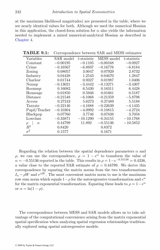
242 Introduction to Spatial Econometrics
at the maximum likelihood magnitudes) are presented in the table, where wesee nearly identical values for both. Although we used the numerical Hessianin this application, the closed-form solution for α also yields the informationneeded to implement a mixed numerical-analytical Hessian as described inChapter 4.
TABLE 9.1: Correspondence between SAR and MESS estimatesVariables SAR model t-statistic MESS model t-statisticConstant −0.00195 −0.1105 −0.00168 −0.0927Crime −0.16567 −6.8937 −0.16776 −6.8184Zoning 0.08057 3.0047 0.07929 2.8732Industry 0.04428 1.2543 0.04670 1.2847Charlesr 0.01744 0.9327 0.01987 1.0406Noxsqr −0.13021 −3.4442 −0.13271 −3.4307Roomsqr 0.16082 6.5430 0.16311 6.4428Houseage 0.01850 0.5946 0.01661 0.5187Distance −0.21548 −6.1068 −0.21359 −5.8798Access 0.27243 5.6273 0.27489 5.5188Taxrate −0.22146 −4.1688 −0.22639 −4.1435Pupil/Teacher −0.10304 −4.0992 −0.10815 −4.2724Blackpop 0.07760 3.7746 0.07838 3.7058Lowclass −0.33871 −10.1290 −0.34155 −10.1768ρ | α 0.44799 11.892 −0.55136 −10.5852R2 0.8420 0.8372σ2 0.1577 0.1671
Regarding the relation between the spatial dependence parameters α andρ, we can use the correspondence, ρ = 1 − eα to transform the value ofα = −0.55136 reported in the table. This results in ρ = 1−e−0.55136 = 0.4238,a value close to the reported SAR estimate of ρ = 0.44799. We derive thiscorrespondence by equating the matrix norms from the two transformationsIn− ρW and eαW . The most convenient matrix norm to use is the maximumrow sum norm which equals 1−ρ for the autoregressive transformation and eα
for the matrix exponential transformation. Equating these leads to ρ = 1−eαor α = ln(1 − ρ).
The correspondence between MESS and SAR models allows us to take ad-vantage of the computational convenience arising from the matrix exponentialspatial specification when analyzing spatial regression relationships tradition-ally explored using spatial autoregressive models.
© 2009 by Taylor & Francis Group, LLC
Matrix Exponential Spatial Models 243
9.2 Spatial error models using MESS
A host of regression models can accommodate spatial dependence in thedisturbances and many of these rely upon particular implementations of mul-tivariate normal regression models. Specifically, given n observations on thedependent variable y and k independent variables X , such models posit alinear (in the parameters) relation among the independent variables as shownin (9.11), where β represents a k element parameter vector and ε follows amultivariate normal distribution with variance-covariance matrix Ω.
y = Xβ + ε (9.11)ε ∼ N (0,Ω)
Models for spatially dependent errors rely on setting Ωij �= 0 when observationi is located near observation j. For example, an externality affecting bothspatial locations i and j could result in εi and εj behaving similarly ( Ωij > 0),the case of positive spatial dependence.
Differences among multivariate normal spatial models arise from alternativespecifications for the variance-covariance matrix Ω. Equation (9.12) showsthe conditional (CSG), simultaneous (SSG), linear moving average (MAL),quadratic moving average (MAQ), and matrix exponential (MESS) specifi-cations using the real scalar parameters φ, λ, γ, θ, α as well as the real n × nspatial weight matrixW .2 We use a symmetricW in this section because CSGand MAL specifications require a symmetric spatial weight matrix. Of course,other spatial specifications can also accommodate symmetric spatial weights,so we rely on this to facilitate comparison of various spatial specifications.
CSG : Ω−1 = In − φW (9.12)SSG : Ω−1 = In − 2ρW + ρ2W 2
MAL : Ω = In + γW
MAQ : Ω = In + 2θW + θ2W 2
MESS : Ω = eαW =∞∑i=0
αiW i
i!
To provide more insight into MESS, consider an expansion of the Taylorseries in (9.12) shown in (9.13).
2Following Cressie (1993) we use SSG in this discussion of error models as a label forsimultaneous autoregressive models. This is to avoid confusion because these are commonlyreferred to as SAR models in the spatial statistics literature. We also use CSG to referencewhat are commonly labeled CAR models in the spatial statistics literature.
© 2009 by Taylor & Francis Group, LLC
244 Introduction to Spatial Econometrics
Ω = In + αW+α2
2W 2 +
α3
6W 3 +
α4
24W 4 +
α5
120W 5 + · · · (9.13)
Ω−1 = In − αW+α2
2W 2 − α3
6W 3 +
α4
24W 4 − α5
120W 5 + · · ·
For positive α and non-negative W , MESS results in non-negative variance-covariance matrix elements, as in the linear (MAL) and quadratic (MAQ)moving average specifications. The inverse of the matrix exponential involvesa simple switch in the sign of α,
((eαW )−1 = e−αW
), so negative α corresponds
to specifying the inverse variance-covariance matrix. For negative values ofα, MESS results in a potential mixture of negative and positive elements asin the SSG specification.
For all specifications either the variance-covariance matrix or the inversevariance-covariance matrix involve powers of the spatial weight matrix in theirTaylor series expansions. These powers have a natural interpretation in thecontext of modeling spatial dependence. For example, positive elements in thesquared weight matrix (W 2)ij > 0 indicate that observation j is a neighbor ofa neighbor to observation i (second-order neighbor). This relation holds forhigher powers of W as well, where non-zero elements of Wh represent h-orderneighbors. Over the relevant parameter domains, all the specifications placelower values on higher-order powers of the spatial weight matrices.
The CSG, SSG, MAL, and MAQ specifications have been mainstays of thespatial dependence literature (Ord, 1975; Anselin, 1988; Ripley, 1988; Hain-ing, 1990). Chiu, Leonard, and Tsui (1996) introduced the matrix exponentialfunction in the context of modeling general non-spatial covariance structures.However, the matrix exponential possesses many desirable properties and ap-pears ideally suited for spatial applications.
First, eαW is positive definite for all α and symmetric W and thus e−αW
is positive definite as well.3 This freedom from singularities greatly simpli-fies both computational and theoretical work. In contrast to MESS, tradi-tional specifications must obey various restrictions to ensure a positive-definitevariance-covariance matrix (Cressie, 1993, p. 468).
Second, since any positive definite matrix is the matrix exponential of somematrix, this means the exponential of some matrix can yield the correctvariance-covariance matrix. In fact, when eαW = Ω, W = α−1 ln (Ω) whereln (·) is the matrix logarithm function (Horn and Johnson, 1994, p. 448, 474).
We can again use the fact that the determinant is a simple function of thetrace |eαW | = eα·tr(W ), and this holds for any real, square matrix (Horn andJohnson, 1994, p. 474). Since the spatial weight matrix W has zeros on thediagonal tr(W ) = 0, resulting in |eαW | = e0 = 1 and ln |Ω (α) | = 0 for allvalues of α. This produces a major simplification as shown by the profile or
3For non-symmetric W , e−α2 W
′e−
α2 W is symmetric positive definite.
© 2009 by Taylor & Francis Group, LLC
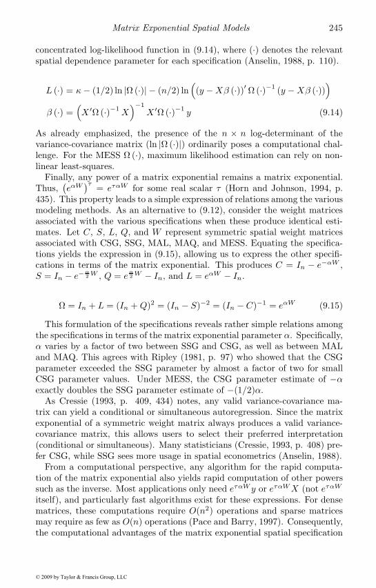
Matrix Exponential Spatial Models 245
concentrated log-likelihood function in (9.14), where (·) denotes the relevantspatial dependence parameter for each specification (Anselin, 1988, p. 110).
L (·) = κ− (1/2) ln |Ω (·)| − (n/2) ln((y −Xβ (·))′ Ω (·)−1 (y −Xβ (·))
)β (·) =
(X ′Ω (·)−1X
)−1
X ′Ω (·)−1 y (9.14)
As already emphasized, the presence of the n × n log-determinant of thevariance-covariance matrix (ln |Ω (·)|) ordinarily poses a computational chal-lenge. For the MESS Ω (·), maximum likelihood estimation can rely on non-linear least-squares.
Finally, any power of a matrix exponential remains a matrix exponential.Thus,
(eαW
)τ = eταW for some real scalar τ (Horn and Johnson, 1994, p.435). This property leads to a simple expression of relations among the variousmodeling methods. As an alternative to (9.12), consider the weight matricesassociated with the various specifications when these produce identical esti-mates. Let C, S, L, Q, and W represent symmetric spatial weight matricesassociated with CSG, SSG, MAL, MAQ, and MESS. Equating the specifica-tions yields the expression in (9.15), allowing us to express the other specifi-cations in terms of the matrix exponential. This produces C = In − e−αW ,S = In − e−
α2W , Q = e
α2W − In, and L = eαW − In.
Ω = In + L = (In +Q)2 = (In − S)−2 = (In − C)−1 = eαW (9.15)
This formulation of the specifications reveals rather simple relations amongthe specifications in terms of the matrix exponential parameter α. Specifically,α varies by a factor of two between SSG and CSG, as well as between MALand MAQ. This agrees with Ripley (1981, p. 97) who showed that the CSGparameter exceeded the SSG parameter by almost a factor of two for smallCSG parameter values. Under MESS, the CSG parameter estimate of −αexactly doubles the SSG parameter estimate of −(1/2)α.
As Cressie (1993, p. 409, 434) notes, any valid variance-covariance ma-trix can yield a conditional or simultaneous autoregression. Since the matrixexponential of a symmetric weight matrix always produces a valid variance-covariance matrix, this allows users to select their preferred interpretation(conditional or simultaneous). Many statisticians (Cressie, 1993, p. 408) pre-fer CSG, while SSG sees more usage in spatial econometrics (Anselin, 1988).
From a computational perspective, any algorithm for the rapid computa-tion of the matrix exponential also yields rapid computation of other powerssuch as the inverse. Most applications only need eταW y or eταWX (not eταW
itself), and particularly fast algorithms exist for these expressions. For densematrices, these computations require O(n2) operations and sparse matricesmay require as few as O(n) operations (Pace and Barry, 1997). Consequently,the computational advantages of the matrix exponential spatial specification
© 2009 by Taylor & Francis Group, LLC
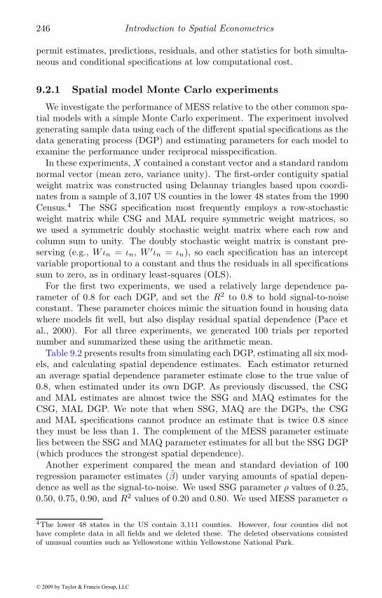
246 Introduction to Spatial Econometrics
permit estimates, predictions, residuals, and other statistics for both simulta-neous and conditional specifications at low computational cost.
9.2.1 Spatial model Monte Carlo experiments
We investigate the performance of MESS relative to the other common spa-tial models with a simple Monte Carlo experiment. The experiment involvedgenerating sample data using each of the different spatial specifications as thedata generating process (DGP) and estimating parameters for each model toexamine the performance under reciprocal misspecification.
In these experiments, X contained a constant vector and a standard randomnormal vector (mean zero, variance unity). The first-order contiguity spatialweight matrix was constructed using Delaunay triangles based upon coordi-nates from a sample of 3,107 US counties in the lower 48 states from the 1990Census.4 The SSG specification most frequently employs a row-stochasticweight matrix while CSG and MAL require symmetric weight matrices, sowe used a symmetric doubly stochastic weight matrix where each row andcolumn sum to unity. The doubly stochastic weight matrix is constant pre-serving (e.g., Wιn = ιn, W ′ιn = ιn), so each specification has an interceptvariable proportional to a constant and thus the residuals in all specificationssum to zero, as in ordinary least-squares (OLS).
For the first two experiments, we used a relatively large dependence pa-rameter of 0.8 for each DGP, and set the R2 to 0.8 to hold signal-to-noiseconstant. These parameter choices mimic the situation found in housing datawhere models fit well, but also display residual spatial dependence (Pace etal., 2000). For all three experiments, we generated 100 trials per reportednumber and summarized these using the arithmetic mean.
Table 9.2 presents results from simulating each DGP, estimating all six mod-els, and calculating spatial dependence estimates. Each estimator returnedan average spatial dependence parameter estimate close to the true value of0.8, when estimated under its own DGP. As previously discussed, the CSGand MAL estimates are almost twice the SSG and MAQ estimates for theCSG, MAL DGP. We note that when SSG, MAQ are the DGPs, the CSGand MAL specifications cannot produce an estimate that is twice 0.8 sincethey must be less than 1. The complement of the MESS parameter estimatelies between the SSG and MAQ parameter estimates for all but the SSG DGP(which produces the strongest spatial dependence).
Another experiment compared the mean and standard deviation of 100regression parameter estimates (β) under varying amounts of spatial depen-dence as well as the signal-to-noise. We used SSG parameter ρ values of 0.25,0.50, 0.75, 0.90, and R2 values of 0.20 and 0.80. We used MESS parameter α
4The lower 48 states in the US contain 3,111 counties. However, four counties did nothave complete data in all fields and we deleted these. The deleted observations consistedof unusual counties such as Yellowstone within Yellowstone National Park.
© 2009 by Taylor & Francis Group, LLC
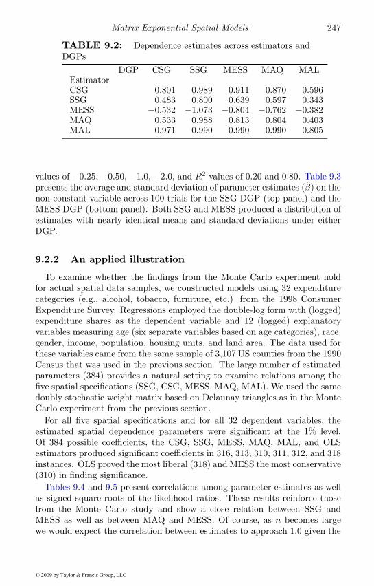
Matrix Exponential Spatial Models 247
TABLE 9.2: Dependence estimates across estimators andDGPs
DGP CSG SSG MESS MAQ MALEstimatorCSG 0.801 0.989 0.911 0.870 0.596SSG 0.483 0.800 0.639 0.597 0.343MESS −0.532 −1.073 −0.804 −0.762 −0.382MAQ 0.533 0.988 0.813 0.804 0.403MAL 0.971 0.990 0.990 0.990 0.805
values of −0.25, −0.50, −1.0, −2.0, and R2 values of 0.20 and 0.80. Table 9.3presents the average and standard deviation of parameter estimates (β) on thenon-constant variable across 100 trials for the SSG DGP (top panel) and theMESS DGP (bottom panel). Both SSG and MESS produced a distribution ofestimates with nearly identical means and standard deviations under eitherDGP.
9.2.2 An applied illustration
To examine whether the findings from the Monte Carlo experiment holdfor actual spatial data samples, we constructed models using 32 expenditurecategories (e.g., alcohol, tobacco, furniture, etc.) from the 1998 ConsumerExpenditure Survey. Regressions employed the double-log form with (logged)expenditure shares as the dependent variable and 12 (logged) explanatoryvariables measuring age (six separate variables based on age categories), race,gender, income, population, housing units, and land area. The data used forthese variables came from the same sample of 3,107 US counties from the 1990Census that was used in the previous section. The large number of estimatedparameters (384) provides a natural setting to examine relations among thefive spatial specifications (SSG, CSG, MESS, MAQ, MAL). We used the samedoubly stochastic weight matrix based on Delaunay triangles as in the MonteCarlo experiment from the previous section.
For all five spatial specifications and for all 32 dependent variables, theestimated spatial dependence parameters were significant at the 1% level.Of 384 possible coefficients, the CSG, SSG, MESS, MAQ, MAL, and OLSestimators produced significant coefficients in 316, 313, 310, 311, 312, and 318instances. OLS proved the most liberal (318) and MESS the most conservative(310) in finding significance.
Tables 9.4 and 9.5 present correlations among parameter estimates as wellas signed square roots of the likelihood ratios. These results reinforce thosefrom the Monte Carlo study and show a close relation between SSG andMESS as well as between MAQ and MESS. Of course, as n becomes largewe would expect the correlation between estimates to approach 1.0 given the
© 2009 by Taylor & Francis Group, LLC
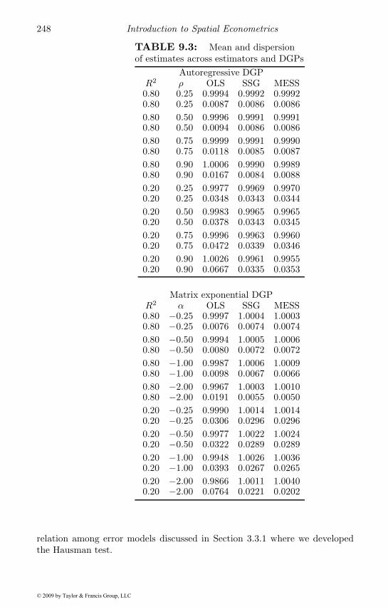
248 Introduction to Spatial Econometrics
TABLE 9.3: Mean and dispersionof estimates across estimators and DGPs
Autoregressive DGPR2 ρ OLS SSG MESS0.80 0.25 0.9994 0.9992 0.99920.80 0.25 0.0087 0.0086 0.00860.80 0.50 0.9996 0.9991 0.99910.80 0.50 0.0094 0.0086 0.00860.80 0.75 0.9999 0.9991 0.99900.80 0.75 0.0118 0.0085 0.00870.80 0.90 1.0006 0.9990 0.99890.80 0.90 0.0167 0.0084 0.00880.20 0.25 0.9977 0.9969 0.99700.20 0.25 0.0348 0.0343 0.03440.20 0.50 0.9983 0.9965 0.99650.20 0.50 0.0378 0.0343 0.03450.20 0.75 0.9996 0.9963 0.99600.20 0.75 0.0472 0.0339 0.03460.20 0.90 1.0026 0.9961 0.99550.20 0.90 0.0667 0.0335 0.0353
Matrix exponential DGPR2 α OLS SSG MESS0.80 −0.25 0.9997 1.0004 1.00030.80 −0.25 0.0076 0.0074 0.00740.80 −0.50 0.9994 1.0005 1.00060.80 −0.50 0.0080 0.0072 0.00720.80 −1.00 0.9987 1.0006 1.00090.80 −1.00 0.0098 0.0067 0.00660.80 −2.00 0.9967 1.0003 1.00100.80 −2.00 0.0191 0.0055 0.00500.20 −0.25 0.9990 1.0014 1.00140.20 −0.25 0.0306 0.0296 0.02960.20 −0.50 0.9977 1.0022 1.00240.20 −0.50 0.0322 0.0289 0.02890.20 −1.00 0.9948 1.0026 1.00360.20 −1.00 0.0393 0.0267 0.02650.20 −2.00 0.9866 1.0011 1.00400.20 −2.00 0.0764 0.0221 0.0202
relation among error models discussed in Section 3.3.1 where we developedthe Hausman test.
© 2009 by Taylor & Francis Group, LLC
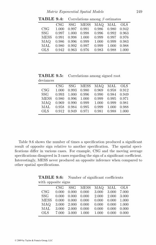
Matrix Exponential Spatial Models 249
TABLE 9.4: Correlations among β estimatesCSG SSG MESS MAQ MAL OLS
CSG 1.000 0.997 0.991 0.986 0.980 0.942SSG 0.997 1.000 0.998 0.996 0.992 0.963MESS 0.991 0.998 1.000 0.999 0.997 0.976MAQ 0.986 0.996 0.999 1.000 0.999 0.983MAL 0.980 0.992 0.997 0.999 1.000 0.988OLS 0.942 0.963 0.976 0.983 0.988 1.000
TABLE 9.5: Correlations among signed rootdeviances
CSG SSG MESS MAQ MAL OLSCSG 1.000 0.993 0.980 0.969 0.958 0.912SSG 0.993 1.000 0.996 0.990 0.984 0.949MESS 0.980 0.996 1.000 0.999 0.995 0.971MAQ 0.969 0.990 0.999 1.000 0.999 0.981MAL 0.958 0.984 0.995 0.999 1.000 0.988OLS 0.912 0.949 0.971 0.981 0.988 1.000
Table 9.6 shows the number of times a specification produced a significantresult of opposite sign relative to another specification. The spatial speci-fications differ in various cases. For example, CSG and the moving averagespecifications disagreed in 3 cases regarding the sign of a significant coefficient.Interestingly, MESS never produced an opposite inference when compared toother spatial specifications.
TABLE 9.6: Number of significant coefficientswith opposite signs
CSG SSG MESS MAQ MAL OLSCSG 0.000 0.000 0.000 3.000 3.000 7.000SSG 0.000 0.000 0.000 2.000 2.000 3.000MESS 0.000 0.000 0.000 0.000 0.000 1.000MAQ 3.000 2.000 0.000 0.000 0.000 1.000MAL 3.000 2.000 0.000 0.000 0.000 0.000OLS 7.000 3.000 1.000 1.000 0.000 0.000
© 2009 by Taylor & Francis Group, LLC
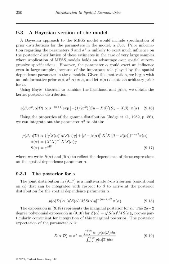
250 Introduction to Spatial Econometrics
9.3 A Bayesian version of the model
A Bayesian approach to the MESS model would include specification ofprior distributions for the parameters in the model, α, β, σ. Prior informa-tion regarding the parameters β and σ2 is unlikely to exert much influence onthe posterior distribution of these estimates in the case of very large sampleswhere application of MESS models holds an advantage over spatial autore-gressive specifications. However, the parameter α could exert an influenceeven in large samples, because of the important role played by the spatialdependence parameter in these models. Given this motivation, we begin withan uninformative prior π(β, σ2|α) ∝ κ, and let π(α) denote an arbitrary priorfor α.
Using Bayes’ theorem to combine the likelihood and prior, we obtain thekernel posterior distribution:
p(β, σ2, α|D) ∝ σ−(n+1)exp[−(1/2σ2)(Sy −Xβ)′(Sy −Xβ)
]π(α) (9.16)
Using the properties of the gamma distribution (Judge et al., 1982, p. 86),we can integrate out the parameter σ2 to obtain:
p(β, α|D) ∝ ([y′S(α)′MS(α)y] + [β − β(α)]′X ′X [β − β(α)])−n/2π(α)β(α) = (X ′X)−1X ′S(α)yS(α) = eαW (9.17)
where we write S(α) and β(α) to reflect the dependence of these expressionson the spatial dependence parameter α.
9.3.1 The posterior for α
The joint distribution in (9.17) is a multivariate t-distribution (conditionalon α) that can be integrated with respect to β to arrive at the posteriordistribution for the spatial dependence parameter α.
p(α|D) ∝ [y′S(α)′MS(α)y]−(n−k)/2π(α) (9.18)
The expression in (9.18) represents the marginal posterior for α. The 2q−2degree polynomial expression in (9.10) for Z(α) = y′S(α)′MS(α)y proves par-ticularly convenient for integration of this marginal posterior. The posteriorexpectation of the parameter α is:
E(α|D) = α∗ =
∫ +∞−∞ α · p(α|D)dα∫ +∞−∞ p(α|D)dα
(9.19)
© 2009 by Taylor & Francis Group, LLC
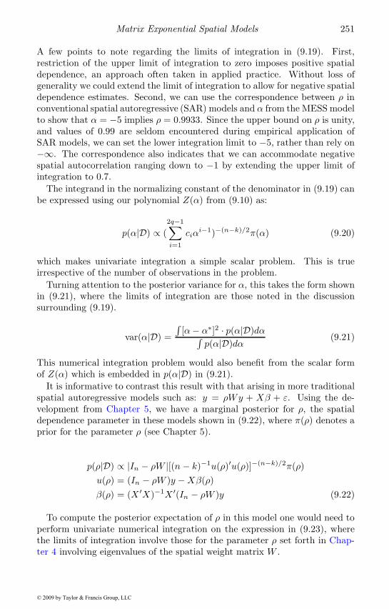
Matrix Exponential Spatial Models 251
A few points to note regarding the limits of integration in (9.19). First,restriction of the upper limit of integration to zero imposes positive spatialdependence, an approach often taken in applied practice. Without loss ofgenerality we could extend the limit of integration to allow for negative spatialdependence estimates. Second, we can use the correspondence between ρ inconventional spatial autoregressive (SAR) models and α from the MESS modelto show that α = −5 implies ρ = 0.9933. Since the upper bound on ρ is unity,and values of 0.99 are seldom encountered during empirical application ofSAR models, we can set the lower integration limit to −5, rather than rely on−∞. The correspondence also indicates that we can accommodate negativespatial autocorrelation ranging down to −1 by extending the upper limit ofintegration to 0.7.
The integrand in the normalizing constant of the denominator in (9.19) canbe expressed using our polynomial Z(α) from (9.10) as:
p(α|D) ∝ (2q−1∑i=1
ciαi−1)−(n−k)/2π(α) (9.20)
which makes univariate integration a simple scalar problem. This is trueirrespective of the number of observations in the problem.
Turning attention to the posterior variance for α, this takes the form shownin (9.21), where the limits of integration are those noted in the discussionsurrounding (9.19).
var(α|D) =∫
[α− α∗]2 · p(α|D)dα∫p(α|D)dα
(9.21)
This numerical integration problem would also benefit from the scalar formof Z(α) which is embedded in p(α|D) in (9.21).
It is informative to contrast this result with that arising in more traditionalspatial autoregressive models such as: y = ρWy + Xβ + ε. Using the de-velopment from Chapter 5, we have a marginal posterior for ρ, the spatialdependence parameter in these models shown in (9.22), where π(ρ) denotes aprior for the parameter ρ (see Chapter 5).
p(ρ|D) ∝ |In − ρW |[(n− k)−1u(ρ)′u(ρ)]−(n−k)/2π(ρ)u(ρ) = (In − ρW )y −Xβ(ρ)β(ρ) = (X ′X)−1X ′(In − ρW )y (9.22)
To compute the posterior expectation of ρ in this model one would need toperform univariate numerical integration on the expression in (9.23), wherethe limits of integration involve those for the parameter ρ set forth in Chap-ter 4 involving eigenvalues of the spatial weight matrix W .
© 2009 by Taylor & Francis Group, LLC
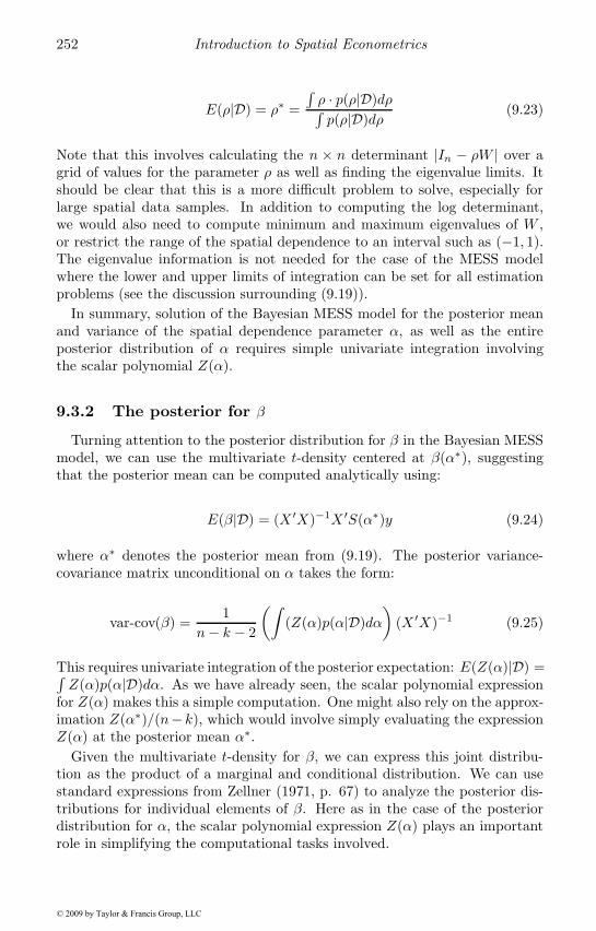
252 Introduction to Spatial Econometrics
E(ρ|D) = ρ∗ =∫ρ · p(ρ|D)dρ∫p(ρ|D)dρ
(9.23)
Note that this involves calculating the n × n determinant |In − ρW | over agrid of values for the parameter ρ as well as finding the eigenvalue limits. Itshould be clear that this is a more difficult problem to solve, especially forlarge spatial data samples. In addition to computing the log determinant,we would also need to compute minimum and maximum eigenvalues of W ,or restrict the range of the spatial dependence to an interval such as (−1, 1).The eigenvalue information is not needed for the case of the MESS modelwhere the lower and upper limits of integration can be set for all estimationproblems (see the discussion surrounding (9.19)).
In summary, solution of the Bayesian MESS model for the posterior meanand variance of the spatial dependence parameter α, as well as the entireposterior distribution of α requires simple univariate integration involvingthe scalar polynomial Z(α).
9.3.2 The posterior for β
Turning attention to the posterior distribution for β in the Bayesian MESSmodel, we can use the multivariate t-density centered at β(α∗), suggestingthat the posterior mean can be computed analytically using:
E(β|D) = (X ′X)−1X ′S(α∗)y (9.24)
where α∗ denotes the posterior mean from (9.19). The posterior variance-covariance matrix unconditional on α takes the form:
var-cov(β) =1
n− k − 2
(∫(Z(α)p(α|D)dα
)(X ′X)−1 (9.25)
This requires univariate integration of the posterior expectation: E(Z(α)|D) =∫Z(α)p(α|D)dα. As we have already seen, the scalar polynomial expression
for Z(α) makes this a simple computation. One might also rely on the approx-imation Z(α∗)/(n− k), which would involve simply evaluating the expressionZ(α) at the posterior mean α∗.
Given the multivariate t-density for β, we can express this joint distribu-tion as the product of a marginal and conditional distribution. We can usestandard expressions from Zellner (1971, p. 67) to analyze the posterior dis-tributions for individual elements of β. Here as in the case of the posteriordistribution for α, the scalar polynomial expression Z(α) plays an importantrole in simplifying the computational tasks involved.
© 2009 by Taylor & Francis Group, LLC
Matrix Exponential Spatial Models 253
9.3.3 Applied illustrations
Three applied illustrations of the Bayesian version of the MESS model areprovided. The first illustration uses a dataset from Pace and Barry (1997)and examines voter turnout in the 1980 presidential election by county for asample of 3,107 US counties and four explanatory variables. A second illus-tration involves 30,987 house sales in Lucas county, Ohio and 10 explanatoryvariables, and the third relies on expenditure budget shares for gasoline in59,025 census tracts with 4 explanatory variables. A standardized first-ordercontiguity matrix was used for the spatial weight matrix W in all illustra-tions. For this application, the matrices W were constructed using Delaunaytriangle algorithms described in Chapter 4 applied to the location coordinatesmeasuring relative position in the map plane.
Estimation results based on maximum likelihood and the Bayesian MESSmodels are presented in Table 9.7. We discuss each of these applications inturn.
For the presidential election example, explanatory variables were: a con-stant term, education (high school graduates), homeownership, and medianhousehold income. The dependent variable is the population voting as a pro-portion of population 19 years or older (those eligible to vote). This proportionwas logged to induce normality. All explanatory variables were expressed aslogs of the population proportion, e.g., the log of homeowners in the countyas a proportion of the county population. A diffuse prior on all parameters,α, β, σ was employed in the Bayesian model, which should produce estimatesnearly identical to those from maximum likelihood estimation.
In the table, we see that Bayesian and maximum likelihood estimates areidentical to at least 3 decimal places in all cases. This similarity of the twosets of estimates also extends to the inferential parameter estimates shownin the table. We used a numerical Hessian evaluation of the log-likelihoodat the ML estimates to produce the standard errors, although one could pro-duce the ML standard errors using the analytic or mixed numerical-analyticHessian described in Chapter 4. The time required to produce estimates forthis 3,107 observation example was 0.110 seconds based on lower and upperintegration limits of −4 and 0 respectively. An important point to note is thata priori knowledge regarding the magnitude of spatial dependence reflectedin the parameter α can be used to further improve the speed of solution. Forexample, setting the lower integration limit to −2 and the upper limit to 0reduced the time needed to solve the problem to 0.08 seconds. Increasing thelimits of integration to −5 and 0 resulted in 0.14 seconds. Varying the limitsof integration produced estimates that were nearly identical. In the table, wereport times based on integration limits of −4 to 0 for timing compatibilityin all three examples.
The second illustration involves a fairly typical housing price model, basedon houses sold over the period from 1993 to 1997 in a single Ohio county.The dependent variable was the log of selling price. Explanatory variables
© 2009 by Taylor & Francis Group, LLC
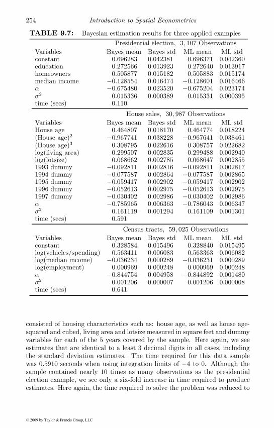
254 Introduction to Spatial Econometrics
TABLE 9.7: Bayesian estimation results for three applied examplesPresidential election, 3, 107 Observations
Variables Bayes mean Bayes std ML mean ML stdconstant 0.696283 0.042381 0.696371 0.042360education 0.272566 0.013923 0.272640 0.013917homeowners 0.505877 0.015182 0.505883 0.015174median income −0.128554 0.016474 −0.128601 0.016466α −0.675480 0.023520 −0.675204 0.023174σ2 0.015336 0.000389 0.015331 0.000395time (secs) 0.110
House sales, 30, 987 ObservationsVariables Bayes mean Bayes std ML mean ML stdHouse age 0.464807 0.018170 0.464774 0.018224(House age)2 −0.967741 0.038228 −0.967641 0.038461(House age)3 0.308795 0.022616 0.308757 0.022682log(living area) 0.299507 0.002835 0.299488 0.002940log(lotsize) 0.068662 0.002785 0.068647 0.0028551993 dummy −0.092811 0.002816 −0.092811 0.0028171994 dummy −0.077587 0.002864 −0.077587 0.0028651995 dummy −0.059417 0.002902 −0.059417 0.0029021996 dummy −0.052613 0.002975 −0.052613 0.0029751997 dummy −0.030402 0.002986 −0.030402 0.002986α −0.785965 0.006363 −0.786043 0.006347σ2 0.161119 0.001294 0.161109 0.001301time (secs) 0.591
Census tracts, 59, 025 ObservationsVariables Bayes mean Bayes std ML mean ML stdconstant 0.328584 0.015496 0.328840 0.015495log(vehicles/spending) 0.563411 0.006083 0.563363 0.006082log(median income) −0.036234 0.000289 −0.036231 0.000289log(employment) 0.000969 0.000248 0.000969 0.000248α −0.844754 0.004958 −0.844892 0.001480σ2 0.001206 0.000007 0.001206 0.000008time (secs) 0.641
consisted of housing characteristics such as: house age, as well as house age-squared and cubed, living area and lotsize measured in square feet and dummyvariables for each of the 5 years covered by the sample. Here again, we seeestimates that are identical to a least 3 decimal digits in all cases, includingthe standard deviation estimates. The time required for this data samplewas 0.5910 seconds when using integration limits of −4 to 0. Although thesample contained nearly 10 times as many observations as the presidentialelection example, we see only a six-fold increase in time required to produceestimates. Here again, the time required to solve the problem was reduced to
© 2009 by Taylor & Francis Group, LLC
Matrix Exponential Spatial Models 255
0.54 seconds when the integration limits were set to −2 and 0, with identicalestimation results.
For the third example using 59,025 census tracts, the relationship exploredinvolved the log share of all expenditures devoted to gasoline on average ineach census tract. One might expect spatial dependence in these observationsas similarly located census tracts would exhibit similar commuting patternsfor work and shopping. A constant term and three explanatory variables wereused: the log budget share of expenditures on vehicles, log median income andlog of employment in the census tract. Here we see a time of 0.641 secondsbased on the integration limits of −4 to 0. In this example, changing the limitsof integration to −2 and 0 had a very modest impact on the time required,reducing it to 0.621 seconds.
9.4 Extensions of the model
We can extend the MESS model to include a more flexible spatial weightspecification that is governed by the introduction of hyperparameters used inthe weight specification. Bayesian MCMC estimation methods can be used toproduce estimates of the hyperparameters that provide information regardingthe nature and extent of spatial influence.
In Section 9.4.1 we introduce this extended version of the model, and in Sec-tion 9.4.2 we describe estimation using Markov Chain Monte Carlo methods.In Section 9.4.3 we illustrate the method in an application.
9.4.1 More flexible weights
Additional flexibility can be introduced by specifying a spatial weight thatincludes a decay parameter φ that lies between 0 and 1, along with a variablenumber of nearest neighbor spatial weight matrices Ni, where the subscripti is used to refer to a weight matrix containing non-zero elements for the ithclosest neighbor. The weight structure specification is shown in (9.26), wherem denotes the maximum number of neighbors considered.
W =m∑i=1
(φiNi∑mi=1 φ
i
)(9.26)
In (9.26), φi weights the relative effect of the ith individual neighbor matrix,so that S depends on the parameters φ as well as m in both its constructionand the metric used. By construction, each row in W sums to 1 and haszeros on the diagonal. To see the role of the spatial decay hyperparameter φ,consider that a value of φ = 0.87 implies a decay profile where the 6th nearestneighbor exerts less than 1/2 the influence of the nearest neighbor. We might
© 2009 by Taylor & Francis Group, LLC
256 Introduction to Spatial Econometrics
think of this value of φ as having a half-life of six neighbors. On the otherhand, a value of φ = 0.95 has a half-life between 14 and 15 neighbors.
The flexibility arising from this type of weight specification adds to theburden of estimation requiring that we draw an inference on the parameters φand m. Together these hyperparameters determine the nature of the spatialweight structure. To the extent that the weight structure specification in(9.26) is flexible enough to adequately approximate more traditional weightmatrices based on contiguity, the model introduced here can replicate resultsfrom models that assume the matrix W is fixed and known. However, allinferences regarding β and σ2 drawn from a model based on a fixed matrixW are conditional on the particular W matrix employed. The model weintroduce here produces inferences regarding β and σ2 that are conditionalonly on a family of spatial weight transformations that we denote Sy, whereS = eαW , with the matricesW taking the form in (9.26). Of course, this raisesthe issue of inference regarding these hyperparameters, and we show that theBayesian MESS model introduced here can produce a posterior distributionfor the joint distribution of the parameters α, φ and m as well as the othermodel parameters of interest, β and σ2.
9.4.2 MCMC estimation
The extended variant of the Bayesian MESS is presented in (9.27), wherethe prior distributions for the parameters are also listed.
Sy = Xβ + ε
S = eαW
W =m∑i=1
(φiNi/
m∑i=1
φi
)ε ∼ N(0, σ2V ), Vii = (v1, . . . , vn), Vij = 0 (i �= j)
π(β) ∼ N(c, T )π(r/vi) ∼ iid χ2(r)π(σ2) ∼ IG(a, b)π(α) ∼ U(−∞, 0]π(φ) ∼ U(0, 1)π(m) ∼ UD[1,mmax] (9.27)
We rely on a normal prior for β ∼ N(c, T ), and inverse gamma prior forσ2, with prior parameters a, b, where the normal and inverse gamma priorsare independent. The prior assigned for α can be a relatively non-informativeuniform prior that allows for the case of no spatial effects when α = 0.
The relative variance terms (v1, v2, . . . , vn) represent our variance scalars toaccommodate outliers and heteroscedasticity as motivated in Chapter 5. We
© 2009 by Taylor & Francis Group, LLC
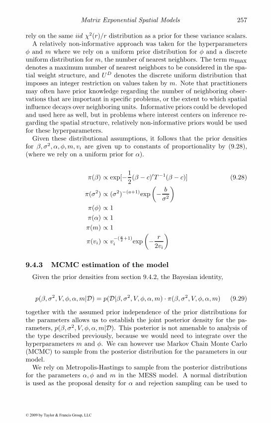
Matrix Exponential Spatial Models 257
rely on the same iid χ2(r)/r distribution as a prior for these variance scalars.A relatively non-informative approach was taken for the hyperparameters
φ and m where we rely on a uniform prior distribution for φ and a discreteuniform distribution for m, the number of nearest neighbors. The term mmaxdenotes a maximum number of nearest neighbors to be considered in the spa-tial weight structure, and UD denotes the discrete uniform distribution thatimposes an integer restriction on values taken by m. Note that practitionersmay often have prior knowledge regarding the number of neighboring obser-vations that are important in specific problems, or the extent to which spatialinfluence decays over neighboring units. Informative priors could be developedand used here as well, but in problems where interest centers on inference re-garding the spatial structure, relatively non-informative priors would be usedfor these hyperparameters.
Given these distributional assumptions, it follows that the prior densitiesfor β, σ2, α, φ,m, vi are given up to constants of proportionality by (9.28),(where we rely on a uniform prior for α).
π(β) ∝ exp[−12(β − c)′T−1(β − c)] (9.28)
π(σ2) ∝ (σ2)−(a+1)exp(− b
σ2
)π(φ) ∝ 1π(α) ∝ 1π(m) ∝ 1
π(vi) ∝ v−( r
2 +1)i exp
(− r
2vi
)
9.4.3 MCMC estimation of the model
Given the prior densities from section 9.4.2, the Bayesian identity,
p(β, σ2, V, φ, α,m|D) = p(D|β, σ2, V, φ, α,m) · π(β, σ2, V, φ, α,m) (9.29)
together with the assumed prior independence of the prior distributions forthe parameters allows us to establish the joint posterior density for the pa-rameters, p(β, σ2, V, φ, α,m|D). This posterior is not amenable to analysis ofthe type described previously, because we would need to integrate over thehyperparameters m and φ. We can however use Markov Chain Monte Carlo(MCMC) to sample from the posterior distribution for the parameters in ourmodel.
We rely on Metropolis-Hastings to sample from the posterior distributionsfor the parameters α, φ and m in the MESS model. A normal distributionis used as the proposal density for α and rejection sampling can be used to
© 2009 by Taylor & Francis Group, LLC
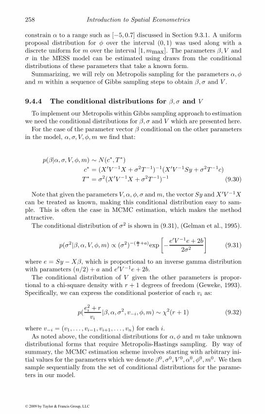
258 Introduction to Spatial Econometrics
constrain α to a range such as [−5, 0.7] discussed in Section 9.3.1. A uniformproposal distribution for φ over the interval (0, 1) was used along with adiscrete uniform for m over the interval [1,mmax]. The parameters β, V andσ in the MESS model can be estimated using draws from the conditionaldistributions of these parameters that take a known form.
Summarizing, we will rely on Metropolis sampling for the parameters α, φand m within a sequence of Gibbs sampling steps to obtain β, σ and V .
9.4.4 The conditional distributions for β, σ and V
To implement our Metropolis within Gibbs sampling approach to estimationwe need the conditional distributions for β, σ and V which are presented here.
For the case of the parameter vector β conditional on the other parametersin the model, α, σ, V, φ,m we find that:
p(β|α, σ, V, φ,m) ∼ N(c∗, T ∗)c∗ = (X ′V −1X + σ2T−1)−1(X ′V −1Sy + σ2T−1c)T ∗ = σ2(X ′V −1X + σ2T−1)−1 (9.30)
Note that given the parameters V, α, φ, σ andm, the vector Sy andX ′V −1Xcan be treated as known, making this conditional distribution easy to sam-ple. This is often the case in MCMC estimation, which makes the methodattractive.
The conditional distribution of σ2 is shown in (9.31), (Gelman et al., 1995).
p(σ2|β, α, V, φ,m) ∝ (σ2)−( n2 +a)exp
[−e
′V −1e+ 2b2σ2
](9.31)
where e = Sy −Xβ, which is proportional to an inverse gamma distributionwith parameters (n/2) + a and e′V −1e+ 2b.
The conditional distribution of V given the other parameters is propor-tional to a chi-square density with r + 1 degrees of freedom (Geweke, 1993).Specifically, we can express the conditional posterior of each vi as:
p(e2i + r
vi|β, α, σ2, v−i, φ,m) ∼ χ2(r + 1) (9.32)
where v−i = (v1, . . . , vi−1, vi+1, . . . , vn) for each i.As noted above, the conditional distributions for α, φ and m take unknown
distributional forms that require Metropolis-Hastings sampling. By way ofsummary, the MCMC estimation scheme involves starting with arbitrary ini-tial values for the parameters which we denote β0, σ0, V 0, α0, φ0,m0. We thensample sequentially from the set of conditional distributions for the parame-ters in our model.
© 2009 by Taylor & Francis Group, LLC
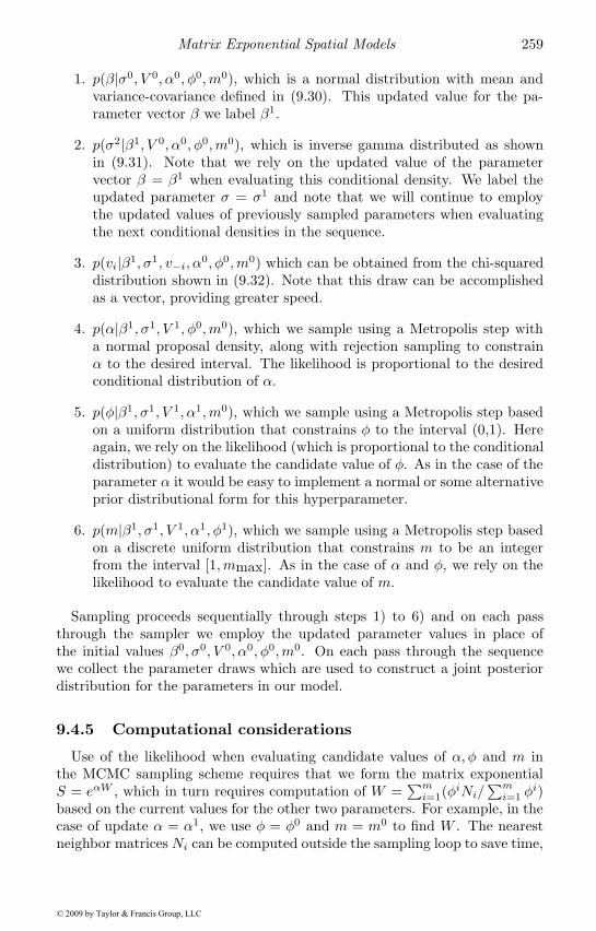
Matrix Exponential Spatial Models 259
1. p(β|σ0, V 0, α0, φ0,m0), which is a normal distribution with mean andvariance-covariance defined in (9.30). This updated value for the pa-rameter vector β we label β1.
2. p(σ2|β1, V 0, α0, φ0,m0), which is inverse gamma distributed as shownin (9.31). Note that we rely on the updated value of the parametervector β = β1 when evaluating this conditional density. We label theupdated parameter σ = σ1 and note that we will continue to employthe updated values of previously sampled parameters when evaluatingthe next conditional densities in the sequence.
3. p(vi|β1, σ1, v−i, α0, φ0,m0) which can be obtained from the chi-squareddistribution shown in (9.32). Note that this draw can be accomplishedas a vector, providing greater speed.
4. p(α|β1, σ1, V 1, φ0,m0), which we sample using a Metropolis step witha normal proposal density, along with rejection sampling to constrainα to the desired interval. The likelihood is proportional to the desiredconditional distribution of α.
5. p(φ|β1, σ1, V 1, α1,m0), which we sample using a Metropolis step basedon a uniform distribution that constrains φ to the interval (0,1). Hereagain, we rely on the likelihood (which is proportional to the conditionaldistribution) to evaluate the candidate value of φ. As in the case of theparameter α it would be easy to implement a normal or some alternativeprior distributional form for this hyperparameter.
6. p(m|β1, σ1, V 1, α1, φ1), which we sample using a Metropolis step basedon a discrete uniform distribution that constrains m to be an integerfrom the interval [1,mmax]. As in the case of α and φ, we rely on thelikelihood to evaluate the candidate value of m.
Sampling proceeds sequentially through steps 1) to 6) and on each passthrough the sampler we employ the updated parameter values in place ofthe initial values β0, σ0, V 0, α0, φ0,m0. On each pass through the sequencewe collect the parameter draws which are used to construct a joint posteriordistribution for the parameters in our model.
9.4.5 Computational considerations
Use of the likelihood when evaluating candidate values of α, φ and m inthe MCMC sampling scheme requires that we form the matrix exponentialS = eαW , which in turn requires computation of W =
∑mi=1(φ
iNi/∑mi=1 φ
i)based on the current values for the other two parameters. For example, in thecase of update α = α1, we use φ = φ0 and m = m0 to find W . The nearestneighbor matrices Ni can be computed outside the sampling loop to save time,
© 2009 by Taylor & Francis Group, LLC

260 Introduction to Spatial Econometrics
but the remaining calculations can still be computationally demanding if thenumber of observations in the problem is large.
Further aggravating this problem is the need to evaluate both the existingvalue of the parameters α, φ and m, given the updated values for β, σ and Vas well as the candidate values. In all, we need to form the matrix productSy, along with the matrix W six times on each pass through the samplingloop.
To enhance the speed of the sampler, we compute the part of Sy thatdepends only on φ and m, for a grid of values over these two parametersprior to beginning the sampler. During evaluation of the conditionals and theMetropolis-Hastings steps, a simple table look-up recovers the stored compo-nent of Sy and applies the remaining calculations needed to fully form Sy.
The ranges for these grids can be specified by the user, with a trade-offbetween selecting a large grid that ensures coverage of the region of posteriorsupport and a narrow grid that requires less time. In a typical spatial problem,the ranges might be 0.5 ≤ φ ≤ 1, and 4 < m < 30. If the grid range is toosmall, the posterior distributions for these parameters should take the formof a censured distribution, indicating inadequate coverage of the region ofsupport.
Simpler models than that presented in (9.27) could be considered. For ex-ample either φ or m, or both φ and m could be fixed a priori. This wouldenhance the speed of the sampler because eliminating one of the two hyper-parameters from the model reduces the computational time needed by almostone-third since it eliminates two of the six computationally intensive stepsinvolving formation of Sy. For example, labels for the various MESS modelsused in the experiments presented in the next section are enumerated belowfrom simplest to most complex.
MESS1 – a model with both ρ and m fixed, and no vi parameters.
MESS2 – a model with ρ fixed, m estimated and no vi parameters.
MESS3 – a model with m fixed, ρ estimated and no vi parameters.
MESS4 – a model with both ρ and m estimated and no vi parameters.
MESS5 – a model with both ρ and m estimated as well as estimates forthe vi parameters.
The use of nearest neighbors also accelerates computation. As described inSection 4.11, nearest neighbor calculations using index arithmetic in place ofmatrix multiplication can greatly reduce computation time as indexing into amatrix is one of the fastest digital operations.
9.4.6 An illustration of the extended model
We provide illustrations of the extended Bayesian MESS model in using agenerated model with only 49 observations taken from Anselin (1988). Use of
© 2009 by Taylor & Francis Group, LLC
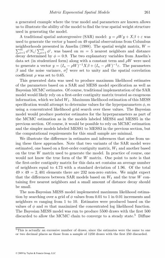
Matrix Exponential Spatial Models 261
a generated example where the true model and parameters are known allowsus to illustrate the ability of the model to find the true spatial weight structureused in generating the model.
A traditional spatial autoregressive (SAR) model: y = ρWy +Xβ + ε wasused to generate the vector y based on 49 spatial observations from Columbusneighborhoods presented in Anselin (1988). The spatial weight matrix, W =∑m
i=1 φiNi/
∑mi=1 φ
i, was based on m = 5 nearest neighbors and distancedecay determined by φ = 0.9. The two explanatory variables from Anselin’sdata set (in studentized form) along with a constant term and ρW were usedto generate a vector y = (In − ρW )−1Xβ + (In − ρW )−1ε. The parametersβ and the noise variance, σ2
ε were set to unity and the spatial correlationcoefficient ρ was set to 0.65.
This generated data was used to produce maximum likelihood estimatesof the parameters based on a SAR and MESS model specification as well asBayesian MCMC estimates. Of course, traditional implementation of the SARmodel would likely rely on a first-order contiguity matrix treated as exogenousinformation, which we labelW1. Maximum likelihood estimation of this MESSspecification would attempt to determine values for the hyperparameters φ,musing a concentrated likelihood grid search over these values. The Bayesianmodel would produce posterior estimates for the hyperparameters as part ofthe MCMC estimation as in the models labeled MESS4 and MESS5 in theprevious section. Of course, it would be possible to rely on MCMC estimationand the simpler models labeled MESS1 to MESS3 in the previous section, butthe computational requirements for this small sample are minimal.
We illustrate the difference in estimates and inferences that arise from us-ing these three approaches. Note that two variants of the SAR model wereestimated, one based on a first-order contiguity matrix, W1 and another basedon the true W matrix used to generate the model. In practice of course, onewould not know the true form of the W matrix. One point to note is thatthe first-order contiguity matrix for this data set contains an average numberof neighbors equal to 4.73 with a standard deviation of 1.96. Of the total49 × 49 = 2, 401 elements there are 232 non-zero entries. We might expectthat the differences between SAR models based on W1 and the true W con-taining five nearest neighbors and a small amount of distance decay shouldbe small.
The non-Bayesian MESS model implemented maximum likelihood estima-tion by searching over a grid of φ values from 0.01 to 1 in 0.01 increments andneighbors m ranging from 1 to 10. Estimates were produced based on thevalues of φ and m that maximized the concentrated log likelihood function.The Bayesian MESS model was run to produce 5500 draws with the first 500discarded to allow the MCMC chain to converge to a steady state.5 Diffuse
5This is actually an excessive number of draws, since the estimates were the same to oneor two decimal places as those from a sample of 1250 draws with the first 250 discarded.
© 2009 by Taylor & Francis Group, LLC
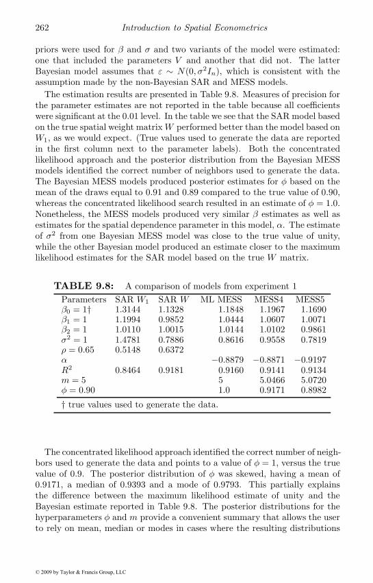
262 Introduction to Spatial Econometrics
priors were used for β and σ and two variants of the model were estimated:one that included the parameters V and another that did not. The latterBayesian model assumes that ε ∼ N(0, σ2In), which is consistent with theassumption made by the non-Bayesian SAR and MESS models.
The estimation results are presented in Table 9.8. Measures of precision forthe parameter estimates are not reported in the table because all coefficientswere significant at the 0.01 level. In the table we see that the SAR model basedon the true spatial weight matrixW performed better than the model based onW1, as we would expect. (True values used to generate the data are reportedin the first column next to the parameter labels). Both the concentratedlikelihood approach and the posterior distribution from the Bayesian MESSmodels identified the correct number of neighbors used to generate the data.The Bayesian MESS models produced posterior estimates for φ based on themean of the draws equal to 0.91 and 0.89 compared to the true value of 0.90,whereas the concentrated likelihood search resulted in an estimate of φ = 1.0.Nonetheless, the MESS models produced very similar β estimates as well asestimates for the spatial dependence parameter in this model, α. The estimateof σ2 from one Bayesian MESS model was close to the true value of unity,while the other Bayesian model produced an estimate closer to the maximumlikelihood estimates for the SAR model based on the true W matrix.
TABLE 9.8: A comparison of models from experiment 1Parameters SAR W1 SAR W ML MESS MESS4 MESS5β0 = 1† 1.3144 1.1328 1.1848 1.1967 1.1690β1 = 1 1.1994 0.9852 1.0444 1.0607 1.0071β2 = 1 1.0110 1.0015 1.0144 1.0102 0.9861σ2 = 1 1.4781 0.7886 0.8616 0.9558 0.7819ρ = 0.65 0.5148 0.6372α −0.8879 −0.8871 −0.9197R2 0.8464 0.9181 0.9160 0.9141 0.9134m = 5 5 5.0466 5.0720φ = 0.90 1.0 0.9171 0.8982
† true values used to generate the data.
The concentrated likelihood approach identified the correct number of neigh-bors used to generate the data and points to a value of φ = 1, versus the truevalue of 0.9. The posterior distribution of φ was skewed, having a mean of0.9171, a median of 0.9393 and a mode of 0.9793. This partially explainsthe difference between the maximum likelihood estimate of unity and theBayesian estimate reported in Table 9.8. The posterior distributions for thehyperparameters φ and m provide a convenient summary that allows the userto rely on mean, median or modes in cases where the resulting distributions
© 2009 by Taylor & Francis Group, LLC
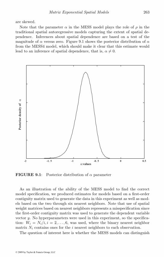
Matrix Exponential Spatial Models 263
are skewed.Note that the parameter α in the MESS model plays the role of ρ in the
traditional spatial autoregressive models capturing the extent of spatial de-pendence. Inferences about spatial dependence are based on a test of themagnitude of α versus zero. Figure 9.1 shows the posterior distribution of αfrom the MESS4 model, which should make it clear that this estimate wouldlead to an inference of spatial dependence, that is, α �= 0.
-2 -1. 5 -1 -0. 5 0 0.5
α values
Po
ster
ior
den
sity
of
α
FIGURE 9.1: Posterior distribution of α parameter
As an illustration of the ability of the MESS model to find the correctmodel specification, we produced estimates for models based on a first-ordercontiguity matrix used to generate the data in this experiment as well as mod-els based on the two through six nearest neighbors. Note that use of spatialweight matrices based on nearest neighbors represents a misspecification sincethe first-order contiguity matrix was used to generate the dependent variablevector y. No hyperparameters were used in this experiment, so the specifica-tion: Wi = Ni/i, i = 2, . . . , 6, was used, where the binary nearest neighbormatrix Ni contains ones for the i nearest neighbors to each observation.
The question of interest here is whether the MESS models can distinguish
© 2009 by Taylor & Francis Group, LLC
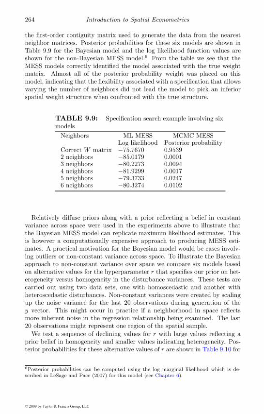
264 Introduction to Spatial Econometrics
the first-order contiguity matrix used to generate the data from the nearestneighbor matrices. Posterior probabilities for these six models are shown inTable 9.9 for the Bayesian model and the log likelihood function values areshown for the non-Bayesian MESS model.6 From the table we see that theMESS models correctly identified the model associated with the true weightmatrix. Almost all of the posterior probability weight was placed on thismodel, indicating that the flexibility associated with a specification that allowsvarying the number of neighbors did not lead the model to pick an inferiorspatial weight structure when confronted with the true structure.
TABLE 9.9: Specification search example involving sixmodels
Neighbors ML MESS MCMC MESSLog likelihood Posterior probability
Correct W matrix −75.7670 0.95392 neighbors −85.0179 0.00013 neighbors −80.2273 0.00944 neighbors −81.9299 0.00175 neighbors −79.3733 0.02476 neighbors −80.3274 0.0102
Relatively diffuse priors along with a prior reflecting a belief in constantvariance across space were used in the experiments above to illustrate thatthe Bayesian MESS model can replicate maximum likelihood estimates. Thisis however a computationally expensive approach to producing MESS esti-mates. A practical motivation for the Bayesian model would be cases involv-ing outliers or non-constant variance across space. To illustrate the Bayesianapproach to non-constant variance over space we compare six models basedon alternative values for the hyperparameter r that specifies our prior on het-erogeneity versus homogeneity in the disturbance variances. These tests arecarried out using two data sets, one with homoscedastic and another withheteroscedastic disturbances. Non-constant variances were created by scalingup the noise variance for the last 20 observations during generation of they vector. This might occur in practice if a neighborhood in space reflectsmore inherent noise in the regression relationship being examined. The last20 observations might represent one region of the spatial sample.
We test a sequence of declining values for r with large values reflecting aprior belief in homogeneity and smaller values indicating heterogeneity. Pos-terior probabilities for these alternative values of r are shown in Table 9.10 for
6Posterior probabilities can be computed using the log marginal likelihood which is de-scribed in LeSage and Pace (2007) for this model (see Chapter 6).
© 2009 by Taylor & Francis Group, LLC
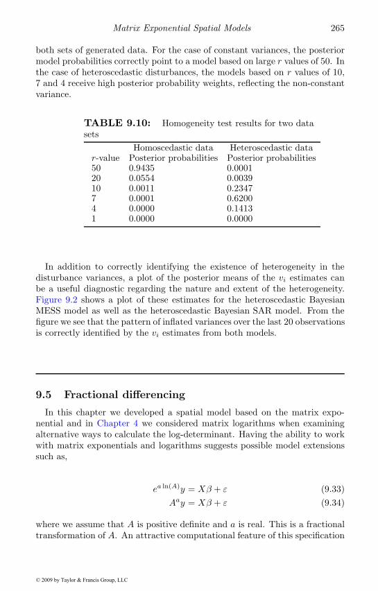
Matrix Exponential Spatial Models 265
both sets of generated data. For the case of constant variances, the posteriormodel probabilities correctly point to a model based on large r values of 50. Inthe case of heteroscedastic disturbances, the models based on r values of 10,7 and 4 receive high posterior probability weights, reflecting the non-constantvariance.
TABLE 9.10: Homogeneity test results for two datasets
Homoscedastic data Heteroscedastic datar-value Posterior probabilities Posterior probabilities50 0.9435 0.000120 0.0554 0.003910 0.0011 0.23477 0.0001 0.62004 0.0000 0.14131 0.0000 0.0000
In addition to correctly identifying the existence of heterogeneity in thedisturbance variances, a plot of the posterior means of the vi estimates canbe a useful diagnostic regarding the nature and extent of the heterogeneity.Figure 9.2 shows a plot of these estimates for the heteroscedastic BayesianMESS model as well as the heteroscedastic Bayesian SAR model. From thefigure we see that the pattern of inflated variances over the last 20 observationsis correctly identified by the vi estimates from both models.
9.5 Fractional differencing
In this chapter we developed a spatial model based on the matrix expo-nential and in Chapter 4 we considered matrix logarithms when examiningalternative ways to calculate the log-determinant. Having the ability to workwith matrix exponentials and logarithms suggests possible model extensionssuch as,
ea ln(A)y = Xβ + ε (9.33)Aay = Xβ + ε (9.34)
where we assume that A is positive definite and a is real. This is a fractionaltransformation of A. An attractive computational feature of this specification
© 2009 by Taylor & Francis Group, LLC
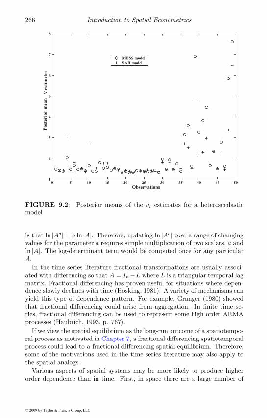
266 Introduction to Spatial Econometrics
0 5 10 15 20 25 30 35 40 45 501
2
3
4
5
6
7
8
Observations
Po
ster
ior
mea
n
V e
stim
ate
s
MESS model
SAR model
FIGURE 9.2: Posterior means of the vi estimates for a heteroscedasticmodel
is that ln |Aa| = a ln |A|. Therefore, updating ln |Aa| over a range of changingvalues for the parameter a requires simple multiplication of two scalars, a andln |A|. The log-determinant term would be computed once for any particularA.
In the time series literature fractional transformations are usually associ-ated with differencing so that A = In−L where L is a triangular temporal lagmatrix. Fractional differencing has proven useful for situations where depen-dence slowly declines with time (Hosking, 1981). A variety of mechanisms canyield this type of dependence pattern. For example, Granger (1980) showedthat fractional differencing could arise from aggregation. In finite time se-ries, fractional differencing can be used to represent some high order ARMAprocesses (Haubrich, 1993, p. 767).
If we view the spatial equilibrium as the long-run outcome of a spatiotempo-ral process as motivated in Chapter 7, a fractional differencing spatiotemporalprocess could lead to a fractional differencing spatial equilibrium. Therefore,some of the motivations used in the time series literature may also apply tothe spatial analogs.
Various aspects of spatial systems may be more likely to produce higherorder dependence than in time. First, in space there are a large number of
© 2009 by Taylor & Francis Group, LLC
Matrix Exponential Spatial Models 267
paths to each observation from every other observation. This means thatchanges in one location could take a very indirect path to influence anotherlocation leading to small amounts of high order dependence. Although in-dividual paths may have a very small influence, the cumulative effect maybe non-trivial. Second, boundaries such as borders and natural features maylead to a reflection of influences, and these influences may not die away asquickly as they would in an infinite, featureless plain. Borders, oceans, rivers,jurisdictions, and other boundaries are integral aspects of the spatial systemand not data artifacts. Complicated geographic features may thus lead tomultiple reflections and high order dependence.
In time series analysis In − L is non-singular, whereas in a spatial settingA = In −W is singular for stochastic W . Although spatial differencing hasappeared in the literature (Ord, 1975), the singular nature of the transforma-tion and its poor empirical performance have not led to much use. However, asmall modification to W can allow for an operation that acts like differencing,but still results in positive definite A.
To see this, consider the usual SAR model in (9.35) where one of the columnsof X equals the unit constant vector ιn. The residuals e in (9.36) result frommultiplying the transformed y by the idempotent matrix MX .
(In − ρW )y = Xβ + ε (9.35)MX(In − ρW )y = e (9.36)
As a brief review of idempotent matrices, for some matrix Z, the matrixHZ = Z(Z ′Z)−1Z ′ is the idempotent projection matrix or Hat matrix, withits complement being the idempotent matrix MZ = In − HZ . Properties ofidempotent matrices include: M2
Z = MZ , H2Z = HZ , and MZHZ = 0n. If Z1
is a subset of Z2, MZ1MZ2 = MZ2MZ1 = MZ2 .Since ιn is a column of X , MXMι = MX . In terms of the Z notation,
Z1 = ιn and Z2 = X . The matrix Mι acts to mean-center columns of matricesor vectors. For example, a regression using an intercept on a variable v yieldsresiduals u with zero mean (u = MXv). This same result could be obtainedby calculating u = MXMιv, since mean-centering a second time still yieldsresiduals with zero mean. The equality in (9.37) arises since MXMι = MX ,
MX(In − ρW )y = MX(In − ρMιW )y (9.37)
Although MιW in (9.37) acts the same as W , In −MιW could be positivedefinite for some forms of W .
Specifically, we introduce a spatial weight matrix W so that In −MιW ispositive definite. One form of W that will produce a positive definite matrixIn −MιW is a symmetric, doubly stochastic weight matrix Wds such that
© 2009 by Taylor & Francis Group, LLC
268 Introduction to Spatial Econometrics
W rds > 0 for some positive integer r.7 This weight matrix has a number
of convenient properties that lead to positive definite In − MιWds. First,because Wds is real and symmetric, Wds = UΛU ′ where U is an n×n matrixof orthogonal eigenvectors and Λ is a real matrix with associated eigenvalueson the diagonal (Horn and Johnson, 1993, 4.1.5). We use ui to denote columni of U or the ith eigenvector. Second, doubly stochastic matrices have amaximum eigenvalue of 1 with a corresponding constant eigenvector (Marcusand Minc, 1992, 5.13.2). Third, since W r
ds > 0 for some positive integer r, thisimplies that the largest eigenvalue of 1 is unique (Horn and Johnson, 1993,Theorem 8.5.2). This condition will be satisfied if there are paths of order ror less between any two entries involved in higher order neighboring relationsspecified by W r
ds.As a result, the doubly stochastic weight matrix Wds has the eigenvalue
expansion shown in (9.38) and (9.39), where the outer product of the firsteigenvector equalsHι and is associated with the maximum eigenvalue, λ1 = 1.
Wds = n−1ιnι′nλ1 + u2u
′2λ2 + . . .+ unu
′nλn (9.38)
Wds = Hιλ1 + u2u′2λ2 + . . .+ unu
′nλn (9.39)
λ1 = max(λ) = 1, abs(λi) < 1 (i = 2, . . . n) (9.40)
Multiplication of Wds by Mι in (9.41) strips away the first eigenvector termassociated with the largest eigenvalue of 1. This defines W−ι where the largestmagnitude eigenvalue is now strictly less than 1 as stated in (9.42).
MιWds = W−ι = u2u′2λ2 + . . .+ unu
′nλn (9.41)
max(abs(λW−ι)) < 1 (9.42)
A brief example may make this clearer. Expression (9.43) presents a sym-metric doubly stochastic matrix W (o)
ds .
W(o)ds =
⎡⎢⎢⎢⎢⎣0.0000 0.3389 0.1895 0.2627 0.20890.3389 0.0000 0.1933 0.1618 0.30600.1895 0.1933 0.0000 0.3538 0.26340.2627 0.1618 0.3538 0.0000 0.22170.2089 0.3060 0.2634 0.2217 0.0000
⎤⎥⎥⎥⎥⎦ (9.43)
The eigenvectors U (o) and the eigenvalues on the diagonal of Λ(o) associatedwith W (o)
ds appear in (9.44) and (9.45).
7Row stochastic matrices could also be used, but these require a more involved developmentbased on the Schur decomposition.
© 2009 by Taylor & Francis Group, LLC
Matrix Exponential Spatial Models 269
U (o) =
⎡⎢⎢⎢⎢⎣0.4472 0.3512 −0.6123 0.5265 0.15680.4472 0.5657 0.0769 −0.5409 −0.42610.4472 −0.5247 0.1534 0.3343 −0.62400.4472 −0.5158 −0.3202 −0.5255 0.39400.4472 0.1237 0.7022 0.2056 0.4993
⎤⎥⎥⎥⎥⎦ (9.44)
diag(Λ(o)) =[1.00 −0.05 −0.19 −0.41 −0.35
](9.45)
The first column of U (o) contains the constant eigenvector, where each of thefive elements equal 0.4472 =
√(1/5), and this eigenvector has an associated
eigenvalue of 1. Multiplication of the constant eigenvector byMι, which mean-centers vectors, essentially eliminates the first eigenvector of U (o), but doesnot change the other eigenvectors. Since the eigenvectors are orthogonal andone of the eigenvectors was a constant vector, the other eigenvectors have azero mean. Multiplication by Mι does not change the other eigenvectors, sothe multiplication MιU
(o) effectively removes the largest eigenvalue of 1 fromW
(o)ds .
MιU(o) =
⎡⎢⎢⎢⎢⎣0.0000 0.3512 −0.6123 0.5265 0.1568
−0.0000 0.5657 0.0769 −0.5409 −0.4261−0.0000 −0.5247 0.1534 0.3343 −0.6240−0.0000 −0.5158 −0.3202 −0.5255 0.3940
0.0000 0.1237 0.7022 0.2056 0.4993
⎤⎥⎥⎥⎥⎦ (9.46)
This allows us to use the matrix W−ι that has a largest eigenvalue less than1 to define a positive definite spatial differencing transformation, Δ−ι, shownin (9.47). We label this term a feasible spatial differencing transformation.The transformation has a log-determinant equal to ψ as indicated in (9.49).
Δ−ι = In −W−ι (9.47)|Δ−ι| = |In −W−ι| > 0 (9.48)
ln |Δ−ι| = ψ (9.49)
Although it is possible to use (9.47) as a feasible spatial differencing trans-formation, it is more flexible to rely on a transformation that introduces areal fractional parameter, δ, as shown in (9.50). Following Hosking (1981),we assume δ ∈ (−0.5, 0.5). An outstanding advantage of the fractional trans-formation is that this leads to a linear log-determinant term in (9.51).
Δδ−ι = eδ ln(Δ−ι) (9.50)
ln |Δδ−ι| = δψ (9.51)
© 2009 by Taylor & Francis Group, LLC
270 Introduction to Spatial Econometrics
In turn, the linear log-determinant term leads to a simple concentrated loglikelihood shown in (9.52).
lnL(δ) = κ+ δψ − n
2ln (e(δ)′e(δ)) (9.52)
e(δ) = MXeδ ln(Δ−ι)y (9.53)
To provide an idea of the performance of spatial fractional feasible differ-encing, we examine two sets of sample data using spatial fractional feasibledifferencing in the next section.
9.5.1 Empirical illustrations
This section provides two illustrations of spatial fractional differencing, onebased on a census tract sample involving housing and the other based on asample of US counties and election data. Use of the smaller sample of UScounties versus the larger sample of US Census tracts should allow variationin the level and relative importance of higher-order spatial dependence.
We compare the fractional differencing method to a variety of other estima-tors. Specifically, for each data set we fitted the model using ordinary least-squares (OLS) as well as moving average (MA), matrix exponential (ME),autoregressive (AR), and fractional differencing (FD) estimators.
(In −W−ι)δy = XβFD + ε1 (9.54)(In − ρW )y = XβAR + ε2 (9.55)
eαW y = XβME + ε3 (9.56)(In − θW )−1y = XβMA + ε4 (9.57)
y = XβOLS + ε5 (9.58)
The motivation for using alternative specifications in the series of exper-iments set forth here is that one approach to accommodating higher-orderspatial dependence would be to rely on alternative model specifications suchas the FD, AR, ME, and MA shown in (9.54)–(9.57).
Another means of capturing neighboring relations is through the weightmatrix, and we use two specifications for W , one based on contiguity withdoubly stochastic scaling that we label (Wc). The second is a weight matrixbased on 30 nearest neighbors with a geometric decay parameter of 0.9 foreach order of neighbor as shown in (9.26). Let Ws = N1+N20.9+N30.81+ . . .where Ni are individual neighbor matrices described in Chapter 4. By itselfWs is non-symmetric. Forming (Ws + W ′
s) and scaling it to make the rowsand columns sum to 1 yields the symmetric doubly stochastic nearest neighbormatrix that we label Wnn.
The experiments will examine whether use of the relatively more sophisti-cated FD model in conjunction with the simpler contiguity weight matrix can
© 2009 by Taylor & Francis Group, LLC
Matrix Exponential Spatial Models 271
produce results comparable to those from simpler model specifications suchas the AR, ME, and MA based on the richer 30 nearest neighbor weight ma-trix. It should be clear that the 30 nearest neighbor weight matrix has moreconnections among neighbors than does a contiguity-based weight matrix.
The experiments will examine the trade-off between specifying dependencevia methods which differ in the emphasis placed on higher-order neighboringrelations versus specifying dependence via weight matrix choice. As will beshown later, ranking methods in terms of the role of high order dependenceyields (from low to high) OLS, MA, MESS, AR, and FD. Intuitively, methodssuch as fractional differencing which allow a role for high order dependencemay prefer a less connected weight matrix such as one based on contiguity.Methods such as moving averages which allow for almost no role for high orderdependence may prefer a more connected weight matrix such as one based onnearest neighbors. Of course, a third modeling strategy is to use both a moresophisticated model and weight matrix in an effort to model higher orderspatial dependence. This is also considered in our experiments.
The first application uses sample data on the votes cast in the 1980 pres-idential election across U.S. counties taken from Pace and Barry (1997). Todetermine the contiguous US counties, we relied on the geographic centroidsof all counties (or their equivalents) from the Census. The dependent variablereflects the total number of recorded votes cast for all parties in the 1980 pres-idential election as a proportion of the voting age population, ln(Votes/Pop)or ln(Votes) − ln(Pop). Explanatory variables used were: the population 18years of age or older (Pop) in each county, the population in each county witha 12th grade or higher education (Education), the number of owner-occupiedhousing units (Houses), and aggregate county-level income (Income). Thesewere used to form the 3, 107 × 5 matrix X shown in (9.59), where we haveadded a constant term vector ιn.
X =[ιn ln(Pop) ln(Education) ln(Houses) ln(Income)
](9.59)
Table 9.11 contains the coefficient and dependence parameter estimatesalong with signed root deviances and log-likelihoods for the various specifica-tions based on the doubly stochastic symmetric contiguity weight matrix, Wc.A clear pattern emerges. Specifically, the log-likelihoods rise as the methodsplace greater emphasis on the role of higher-order neighboring relations withfractional differencing producing the highest log likelihood and OLS the low-est log likelihood. In addition, the fractionally differenced method produceda material improvement in log-likelihood function values, achieving a valuethat is 92.9 higher than its nearest competitor, the AR model.
Table 9.12 contains the coefficient estimates along with signed root de-viances and log-likelihoods for the various specifications based on the dou-bly stochastic symmetric nearest neighbor weight matrix, Wnn. Table 9.12shows that every spatial specification except fractional differencing displayeda higher likelihood for the nearest neighbor weight matrix Wnn relative to a
© 2009 by Taylor & Francis Group, LLC
272 Introduction to Spatial Econometrics
contiguity based weight matrix Wc. This result is consistent with the notionthat a richer weight matrix specification should improve the model estimatesfrom methods that place less emphasis on higher order neighboring relations.These results produced a higher concentrated-log likelihood function value forthe AR specification than the fractional differencing specification. However,the geometric parameter used to create the weight matrix was set to maximizeperformance of the AR specification. Relative to the fractional differencingresults based on the contiguity-based weight matrix, here we find that an ARspecification based on the nearest neighbor weight matrix produced the high-est likelihood. However, the small difference of 6.21 between log likelihoodsmay be partially due to fitting the geometric parameter governing the weightsassigned to individual neighbors.
Another interesting pattern emerges from comparing the coefficient esti-mates from Table 9.11 and Table 9.12. If we compare the AR estimates as wemove from contiguity (Wc) to nearest neighbor weights (Wnn) , these movetoward the FD estimates based on contiguity (Wc). This suggests that the FDmodel is better capable of using the simpler contiguity weight matrix (Wc) tocapture patterns of higher-order spatial dependence relative to the AR modelusing Wc.
The second application uses housing data. Housing provides a classic ex-ample of spatially dependent data, and we examine (logged) housing valuesas a function of (logged) households, median household income, median yearsof education, and land area. The sample data represent 62, 226 census-tractlevel observations from the 2000 Census. This application uses the definitionof X from (9.60).
X =[ιn ln(Households) ln(Income) ln(Education) ln(Land Area)
](9.60)
Table 9.13 contains the coefficient and dependence estimates along withsigned root deviances and log-likelihoods for the various specifications basedon the doubly stochastic symmetric contiguity weight matrix, Wc. Like thecounty-level election data results, Table 9.13 again shows a pattern wherethe log-likelihood rises as each method places more emphasis on higher or-der dependence (FD>AR>ME>MA>OLS). The difference between log like-lihoods is material with FD exceeding the likelihood of the AR specificationby 2, 588.60.
Table 9.14 contains results for the various specifications based on the dou-bly stochastic symmetric nearest neighbor weight matrix, Wnn in the sameformat as Table 9.13. We see a similar pattern to those from the electiondata, with the AR specification exhibiting the highest likelihood. In this case,the log-likelihood from the ME specification also exceeded the FD log likeli-hood, but unlike the election data example, FD using the simpler contiguityweight matrix Wc outperformed an AR specification based on the richer 30nearest neighbors weight matrix. This makes the point that the FD model
© 2009 by Taylor & Francis Group, LLC
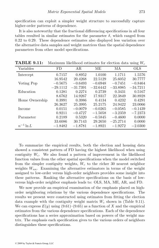
Matrix Exponential Spatial Models 273
specification can exploit a simpler weight structure to successfully capturehigher-order patterns of dependence.
It is also noteworthy that the fractional differencing specifications in all fourtables resulted in similar estimates for the parameter δ, which ranged from0.22 to 0.29. These dependence estimates also displayed less variation overthe alternative data samples and weight matrices than the spatial dependenceparameters from other model specifications.
TABLE 9.11: Maximum likelihood estimates for election data using Wc
Variables FD AR ME MA OLS
Intercept 0.7157 0.8952 1.0100 1.1711 1.557616.9542 20.4268 22.5129 25.6052 30.7777
Voting Pop −0.5675 −0.6493 −0.6948 −0.7451 −0.8464−29.1112 −31.7391 −32.6442 −33.8985 −34.7211
Education 0.1281 0.2274 0.2739 0.3431 0.51678.6762 14.9267 17.9317 22.3849 30.8928
Home Ownership 0.3991 0.3986 0.4134 0.4232 0.429126.3627 25.3995 25.2175 24.9422 23.0066
Income 0.0151 −0.0079 −0.0265 −0.0585 −0.14390.9211 −0.4727 −1.5058 −3.2359 −7.2373
Parameter 0.2189 0.5320 −0.5845 −0.4600 0.000033.6086 30.7143 29.2650 −25.2714 0.0000
n−1 lnL −1.8482 −1.8781 −1.8921 −1.9272 −2.0300
To summarize the empirical results, both the election and housing datashowed a consistent pattern of FD having the highest likelihood when usingcontiguity Wc. We also found a pattern of improvement in the likelihoodfunction values from the other spatial specifications when the model switchedfrom the simpler contiguity weights, Wc to the richer 30 nearest neighborweights Wnn. Examining the alternative estimators in terms of the weightassigned to low-order versus high-order neighbors provides some insight intothese patterns. Ranking the alternative specifications on the basis of low-versus high-order neighbor emphasis leads to: OLS, MA, ME, AR, and FD.
We now provide an empirical examination of the emphasis placed on high-order neighboring relations by the various dependence specifications. Theresults we present were constructed using estimates from fitting the electiondata example with the contiguity weight matrix Wc shown in (Table 9.11).We can express E(y) using (9.61)–(9.65) as a function of X and the empiricalestimates from the various dependence specifications. Each of the dependencespecifications has a series approximation based on powers of the weight ma-trix. The emphasis each specification gives to the various orders of neighborsdistinguishes these specifications.
© 2009 by Taylor & Francis Group, LLC
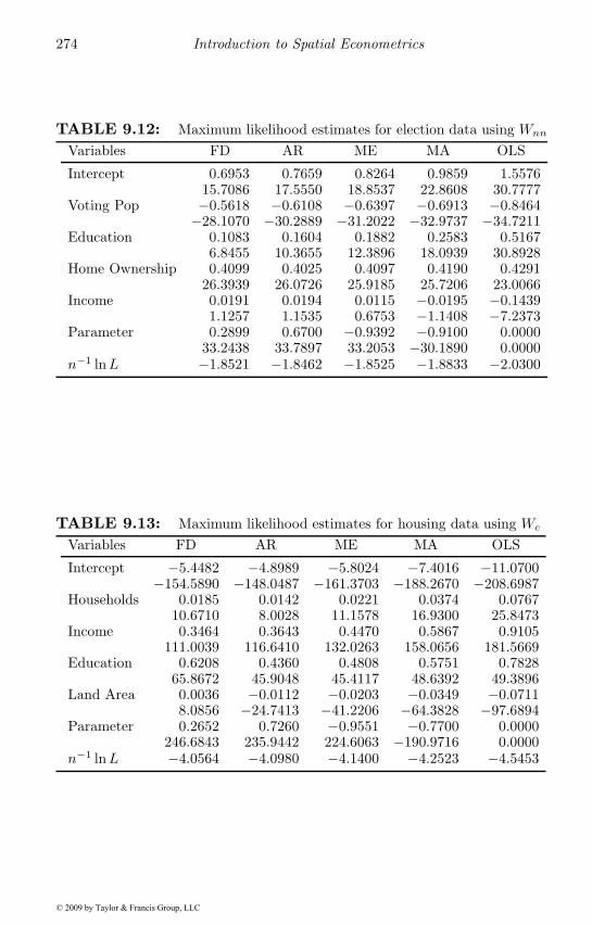
274 Introduction to Spatial Econometrics
TABLE 9.12: Maximum likelihood estimates for election data using Wnn
Variables FD AR ME MA OLS
Intercept 0.6953 0.7659 0.8264 0.9859 1.557615.7086 17.5550 18.8537 22.8608 30.7777
Voting Pop −0.5618 −0.6108 −0.6397 −0.6913 −0.8464−28.1070 −30.2889 −31.2022 −32.9737 −34.7211
Education 0.1083 0.1604 0.1882 0.2583 0.51676.8455 10.3655 12.3896 18.0939 30.8928
Home Ownership 0.4099 0.4025 0.4097 0.4190 0.429126.3939 26.0726 25.9185 25.7206 23.0066
Income 0.0191 0.0194 0.0115 −0.0195 −0.14391.1257 1.1535 0.6753 −1.1408 −7.2373
Parameter 0.2899 0.6700 −0.9392 −0.9100 0.000033.2438 33.7897 33.2053 −30.1890 0.0000
n−1 lnL −1.8521 −1.8462 −1.8525 −1.8833 −2.0300
TABLE 9.13: Maximum likelihood estimates for housing data using Wc
Variables FD AR ME MA OLS
Intercept −5.4482 −4.8989 −5.8024 −7.4016 −11.0700−154.5890 −148.0487 −161.3703 −188.2670 −208.6987
Households 0.0185 0.0142 0.0221 0.0374 0.076710.6710 8.0028 11.1578 16.9300 25.8473
Income 0.3464 0.3643 0.4470 0.5867 0.9105111.0039 116.6410 132.0263 158.0656 181.5669
Education 0.6208 0.4360 0.4808 0.5751 0.782865.8672 45.9048 45.4117 48.6392 49.3896
Land Area 0.0036 −0.0112 −0.0203 −0.0349 −0.07118.0856 −24.7413 −41.2206 −64.3828 −97.6894
Parameter 0.2652 0.7260 −0.9551 −0.7700 0.0000246.6843 235.9442 224.6063 −190.9716 0.0000
n−1 lnL −4.0564 −4.0980 −4.1400 −4.2523 −4.5453
© 2009 by Taylor & Francis Group, LLC
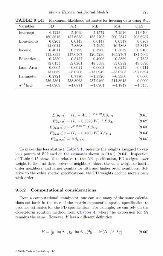
Matrix Exponential Spatial Models 275
TABLE 9.14: Maximum likelihood estimates for housing data using Wnn
Variables FD AR ME MA OLS
Intercept −6.4223 −5.4099 −5.4572 −7.2926 −11.0700−160.8616 −157.6558 −155.2703 −200.2547 −208.6987
Households 0.0263 0.0143 0.0147 0.0347 0.076714.0014 7.8368 7.7959 16.7868 25.8473
Income 0.4011 0.3799 0.3960 0.5639 0.9105113.8333 117.0507 120.5236 165.2767 181.5669
Education 0.7350 0.5157 0.4906 0.5869 0.782872.0133 52.6201 48.5588 53.0282 49.3896
Land Area 0.0065 −0.0024 −0.0063 −0.0272 −0.071113.0689 −5.0206 −13.0949 −55.0203 −97.6894
Parameter 0.2721 0.7770 −1.3320 −0.9900 0.0000236.2361 238.8063 237.9460 −211.8613 0.0000
n−1 lnL −4.0969 −4.0871 −4.0904 −4.1847 −4.5453
E(yFD) = (In −W−ι)−0.2189XβFD (9.61)E(yAR) = (In − 0.5320 W )−1XβAR (9.62)
E(yME)y = e0.5845 WXβME (9.63)E(yMA)y = (In + 0.4600 W )XβMA (9.64)E(yOLS) = XβOLS (9.65)
To make this less abstract, Table 9.15 presents the weights assigned to var-ious powers of W based on the estimates shown in (9.61)–(9.64). Inspectionof Table 9.15 shows that relative to the AR specification, FD assigns lowerweight to the first three orders of neighbors, about the same weight to fourthorder neighbors, and larger weights for fifth and higher order neighbors. Rel-ative to the other spatial specifications, the FD weights decline more slowlywith order.
9.5.2 Computational considerations
From a computational standpoint, one can use many of the same calcula-tions set forth in the case of the matrix exponential spatial specification toproduce estimates for the FD specification. For example, we can rely on theclosed-form solution method from Chapter 4, where the expression for G1
remains the same. However, Y has a different definition.
Y =[y ln(Δ−ι)y ln(Δ−ι)2y . . . ln(Δ−ι)q−1y
](9.66)
© 2009 by Taylor & Francis Group, LLC
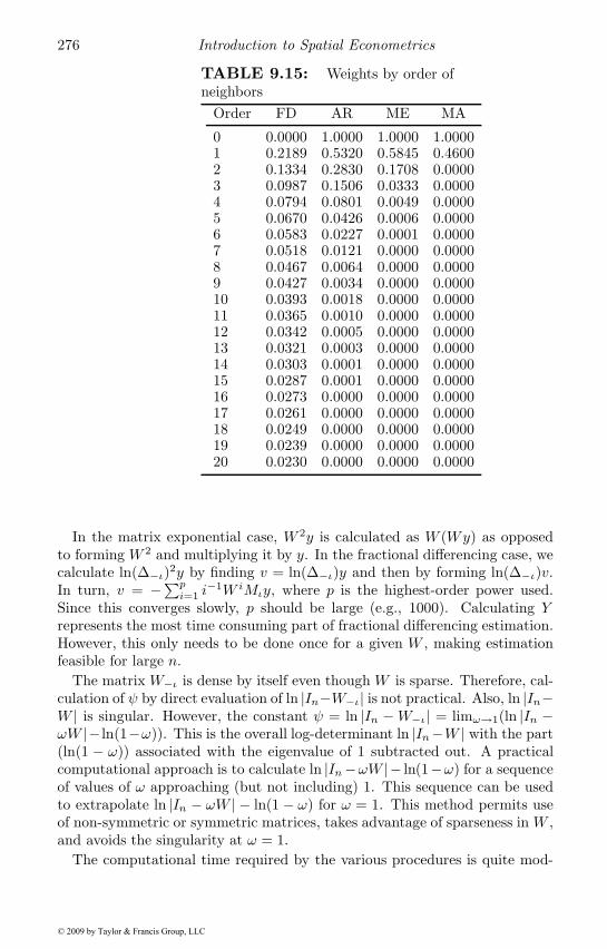
276 Introduction to Spatial Econometrics
TABLE 9.15: Weights by order ofneighbors
Order FD AR ME MA
0 0.0000 1.0000 1.0000 1.00001 0.2189 0.5320 0.5845 0.46002 0.1334 0.2830 0.1708 0.00003 0.0987 0.1506 0.0333 0.00004 0.0794 0.0801 0.0049 0.00005 0.0670 0.0426 0.0006 0.00006 0.0583 0.0227 0.0001 0.00007 0.0518 0.0121 0.0000 0.00008 0.0467 0.0064 0.0000 0.00009 0.0427 0.0034 0.0000 0.000010 0.0393 0.0018 0.0000 0.000011 0.0365 0.0010 0.0000 0.000012 0.0342 0.0005 0.0000 0.000013 0.0321 0.0003 0.0000 0.000014 0.0303 0.0001 0.0000 0.000015 0.0287 0.0001 0.0000 0.000016 0.0273 0.0000 0.0000 0.000017 0.0261 0.0000 0.0000 0.000018 0.0249 0.0000 0.0000 0.000019 0.0239 0.0000 0.0000 0.000020 0.0230 0.0000 0.0000 0.0000
In the matrix exponential case, W 2y is calculated as W (Wy) as opposedto forming W 2 and multiplying it by y. In the fractional differencing case, wecalculate ln(Δ−ι)2y by finding v = ln(Δ−ι)y and then by forming ln(Δ−ι)v.In turn, v = −∑p
i=1 i−1W iMιy, where p is the highest-order power used.
Since this converges slowly, p should be large (e.g., 1000). Calculating Yrepresents the most time consuming part of fractional differencing estimation.However, this only needs to be done once for a given W , making estimationfeasible for large n.
The matrix W−ι is dense by itself even though W is sparse. Therefore, cal-culation of ψ by direct evaluation of ln |In−W−ι| is not practical. Also, ln |In−W | is singular. However, the constant ψ = ln |In −W−ι| = limω→1(ln |In −ωW |− ln(1−ω)). This is the overall log-determinant ln |In−W | with the part(ln(1 − ω)) associated with the eigenvalue of 1 subtracted out. A practicalcomputational approach is to calculate ln |In−ωW |− ln(1−ω) for a sequenceof values of ω approaching (but not including) 1. This sequence can be usedto extrapolate ln |In − ωW | − ln(1 − ω) for ω = 1. This method permits useof non-symmetric or symmetric matrices, takes advantage of sparseness in W ,and avoids the singularity at ω = 1.
The computational time required by the various procedures is quite mod-
© 2009 by Taylor & Francis Group, LLC
Matrix Exponential Spatial Models 277
erate. For the n = 3, 107 data set it took 0.2 seconds to find the contiguityweight matrix, 0.06 seconds to calculate ψ, 9.61 seconds to compute Y (forp = 2, 500, q = 16) and only 0.13 seconds to produce the fractional differenc-ing estimates. The 30 nearest neighbor case required 0.47 seconds to find theweight matrix, 0.28 seconds to compute ψ, 19.84 seconds to compute Y , and0.14 seconds to find the estimates.8 We need only form ψ and Y when chang-ing W , and thus exploring models based on alternative independent variablesrequires very little computational time.
As a check on this approach to calculating ψ, we found the eigenvalues ofWc for the election data and calculated the log-determinant of W−ι directly.The difference between the log-determinant from the eigenvalue calculationand the proposed approach was 0.0054, a very small number. We also checkedthe accuracy of the fractional differencing approximation. This was done bychanging p, the degree of the matrix logarithm approximation, and q, thedegree of the matrix exponential approximation. Changing p and q had someeffect on the accuracy of δ, and therefore on the regression coefficients. Forthe election data using Wc, changing from p = 1, 000 and q = 8 to p = 2, 500and q = 16 resulted in a change in the δ estimate from 0.2197 to 0.2189, adifference of 0.0008.
For the larger n = 62, 226 data set, it took 2.4 seconds to form the spatialweight matrix, 0.80 seconds to determine ψ, 4.65 minutes to compute Y usingq = 16 and p = 2, 500, and only 0.17 seconds to find the fractional differencingestimates. The 30 nearest neighbor case required 6.03 seconds for ψ, and 13.47minutes to compute Y . Again, when changing X the marginal computationalcost would just be the time to find the fractional differencing estimates. Thekey computational burden is computing Y , and this could be reduced by goingto a Chebyshev approximation of the type described in Chapter 4.
9.6 Chapter summary
We have introduced the matrix exponential spatial specification (MESS)as an alternative to the spatial autoregressive process. MESS can be usedto construct spatial regression models that replace geometric decay from thespatial autoregressive process with exponential decay.
This type of specification has both computational as well as theoretical ad-vantages over the spatial autoregressive specification. These arise from theease of inversion, differentiation, and integration of the matrix exponential.Moreover, the covariance matrix associated with the matrix exponential isalways positive definite. Finally, the matrix exponential has a simple matrix
8All the times were for a machine using an AMD 3.2 Ghz Athlon.
© 2009 by Taylor & Francis Group, LLC
278 Introduction to Spatial Econometrics
determinant which vanishes for the common case of a spatial weight matrixwith a trace of zero. This simplification was used to produce a closed-formsolution for maximum likelihood estimates, and to provide Bayesian estimatesbased on univariate numerical integration of a scalar polynomial expression.In addition, some of the benefits of MESS extend to the case of spatial frac-tional differencing.
LeSage and Pace (2007) provide a further illustration that demonstrateshow the analytical and computational advantages of MESS can be exploited inBayesian model comparisonMC3 methods of the type described in Chapter 6.The MC3 method was implemented by drawing on straightforward extensionsof the existing results in the regression model literature.
The chapter also set forth a spatial specification based on a fractional differ-encing transformation. In the time series literature fractional differencing hasproven useful in situations where dependence slowly declines with time. Weargued that spatial systems may be more likely to produce patterns of higherorder dependence than in the case of time series analysis. This type of pat-tern seems likely to arise when the number of connection paths between eachobservation and all others is large, or when boundaries or borders producemultiple reflections as a result of changes to nodes in the system.
© 2009 by Taylor & Francis Group, LLC
Chapter 10
Limited Dependent Variable SpatialModels
This chapter introduces approaches to modeling dependent variables that re-flect binary choice outcomes generated by spatially dependent processes. Spa-tial dependence in choice outcomes result in a situation where observed choicesat one location are similar to choices made at nearby locations. There are anumber of scenarios where we might see this type of outcome in observedchoices. For example, in the aftermath of Hurricane Katrina the decision ofa business owner in New Orleans to rebuild and reopen a store might de-pend on the decision of neighboring businesses to reopen. When consideringorigin-destination flows of commuters traveling to work, the choice betweenmass transit and automobile mode of travel might exhibit spatial dependencebecause commuters located at nearby origins would be faced with the samepresence or absence of mass transit opportunities. Holloway, Shankara, andRahman (2002) show that binary choices regarding adoption of an agricul-tural program by Bangladeshi rice producers exhibited spatial dependence.Applications to land-use decisions regarding conversion from agricultural tonon-agricultural uses, where land-use decisions of neighboring property own-ers exert an influence on the decision outcome have also been popular (Zhouand Kockelman, 2008; Irwin and Bockstael, 2004). Probit variants of the SARmodel were considered by McMillen (1992), who proposed an EM algorithm asa way to produce consistent (maximum likelihood) measures of dispersion forestimates β from these models. A major contribution to the non-spatial probitliterature was the work of Albert and Chib (1993) who proposed treating thebinary dependent variable observations as indicators that relate to underlyingunobservable or latent levels of utility. They introduce these latent levels asparameters that can be estimated using a Bayesian MCMC framework. Wediscuss this type of approach in Section 10.1 which we extend to the case ofthe spatial probit SAR model (LeSage, 2000). We consider a related Tobit(or censored regression) model variant of the SAR model in Section 10.3.
The first type of spatial probit model that we discuss takes the SAR formshown in (10.1), where the n× 1 vector y contains a set of 0,1 binary valuesthat reflect choice outcomes, or they might reflect presence or absence of a taxor other feature in each region/observation. We could also have a measure ofnegative or positive change in (average) land values for a sample of regions,and so on.
279© 2009 by Taylor & Francis Group, LLC
280 Introduction to Spatial Econometrics
y = ρWy +Xβ + ε, ε ∼ N(0, σ2εIn) (10.1)
This probit variant of the SAR model could of course be extended to thecase of the SDM model by adding spatial lags of the explanatory variables.The motivations for a spatial lag of the dependent variable already describedin the initial chapters should apply here as well. For example, if we beginwith a time-lagged model that relates yt to Wyt−1, then we are stating thatdecision outcomes (or the presence or absence of some feature in each region)exert an impact on future decisions (or features) of neighboring regions.
Similarly, beginning with a non-spatial relationship: y = Xβ+u, our moti-vation for a spatial lag of the dependent variable as arising from the presenceof an omitted variable that is correlated with an included variable and ex-hibits spatial dependence would also provide a motivation for the SAR orSDM model. As an example, if we have a binary measure of the presence orabsence of patenting activity for a sample of regions, the existence of tacit un-measurable knowledge that is excluded from the set of explanatory variablesin the model should lead to spatial dependence in the observed measures thatrecord the presence or absence of regional patenting activity.
In addition to the SAR probit model we also discuss SAR ordered probit,SAR Tobit, and SAR multinomial probit variants of the SAR probit model.We approach the estimation task from a Bayesian MCMC sampling viewpoint.For an extensive discussion of alternative approaches to estimating these mod-els see Flemming (2004). Maximum likelihood estimation seems quite difficultas pointed out by Beron and Vijverberg (2000), who report estimation timesfor a SAR probit model requiring many hours for a 49 observation problem.Early use of Bayesian MCMC sampling for spatial probit models can be foundin Bolduc, Fortin and Gordon (1997), who model a spatial error covariancestructure.
A second type of model that we explore in Section 10.6 was introducedby Smith and LeSage (2004). This model relies on an error structure thatinvolves an additive error specification first introduced by Besag, York andMollie (1991) and subsequently employed by many authors (Gelman et al.,1995). The approach of Smith and LeSage (2004) allows both spatial depen-dencies and general spatial heteroscedasticity to be treated simultaneouslyand has been popular in marketing applications (Allenby et al., 2002; Yangand Allenby, 2003; Ter Hofstede, Wedel and Steenkamp, 2002).
Smith and LeSage (2004) illustrate the method using county-level votingoutcomes for a presidential election. The model relies on spatially structuredeffects parameters as well as common variance scalars for broader regions suchas states in the county-level voting application. This allows for state-leveldifferences in the effects parameters as well as the variance.
Section 10.6 also discusses a dynamic spatial ordered probit extension of thismodel described in Wang and Kockelman (2008a,b). This dynamic variant
© 2009 by Taylor & Francis Group, LLC
Limited Dependent Variable Spatial Models 281
of the model can capture patterns of spatial and temporal autocorrelation inordered categorical response data.
The next section begins with a discussion of Bayesian treatment of unob-served latent utilities, which is a key feature of MCMC estimation of probit,tobit and multinomial probit models.
10.1 Bayesian latent variable treatment
The Bayesian approach to modeling binary limited dependent variablestreats the binary 0,1 observations in y as indicators of latent, unobserved (net)utility. The unobservable utility underlies the observed choice outcomes. Forexample, if the binary dependent variable reflects the decision to buy or notbuy a product, the observed 0,1 indicator variable y represents observed de-cision outcomes in our sample. These are viewed as merely a proxy for thefact that when net utility is negative, a decision not to buy (y = 0) is made,and when net utility associated with the purchase is positive, a buy decision(y = 1) is made.1 The Bayesian estimation approach to these models is toreplace the unobserved latent utility with parameters that are estimated. Forthe case of a SAR probit model, given estimates of the n× 1 vector of miss-ing or unobserved (parameter) values that we denote as y∗, we can proceedto estimate the remaining model parameters β, ρ by sampling from the sameconditional distributions that we used in the continuous dependent variableBayesian SAR models from Chapter 5.
More formally, the choice depends on the difference in utilities: (U1i −U0i), i = 1, . . . , n associated with observed 0,1 choice indicators. The probitmodel assumes this difference, y∗i = U1i − U0i, follows a normal distribution.We do not observe y∗i , only the choices made, which are reflected in:
yi = 1, if y∗i ≥ 0yi = 0, if y∗i < 0
There are strict interpretations of this relationship that rely on utility max-imization to argue that an individual located in region i choosing alternative1 implies: Pr(yi = 1) = Pr(U1i ≥ U0i) = Pr(y∗i ≥ 0). Smith and LeSage(2004) provide a more detailed discussion of these issues. Albert and Chib(1993) adopt a less formal economic interpretation and view the y∗i as simplyunobserved values associated with observed choice events. These are modeledusing the non-spatial regression relation: y∗i = Xiβ + εi, εi ∼ N(0, σ2
ε).
1The utility derived from owning the good could be considered minus that from retainingincome equal to the purchase price when the consumer does not buy the good.
© 2009 by Taylor & Francis Group, LLC
282 Introduction to Spatial Econometrics
If the vector of latent utilities y∗ were known, we would also know y, whichled Albert and Chib (1993) to conclude: p(β, σ2
ε |y∗) = p(β, σ2ε |y∗, y). The
insight here is that if we view y∗ as an additional set of parameters to be es-timated, then the (joint) conditional posterior distribution for the model pa-rameters β, σ2
ε (conditioning on both y∗, y) takes the same form as a Bayesianregression problem involving a continuous dependent variable rather than theproblem involving the discrete-valued vector y. We extend this approach tothe case of a SAR model where the model parameters are β, ρ, σ2
ε . If an ad-ditional set of n parameters y∗i , i = 1, . . . , n were introduced to the model,estimation via MCMC sampling would require that we sequentially sampleeach of these parameters from their conditional distributions. Recall that ourMCMC estimation scheme for the SAR model simply cycles through the se-quence of conditional distributions for all model parameters taking samplesfrom each of these. A large number of passes through the sampler produces asequence of draws for the model parameters that converge to the unconditionaljoint posterior distribution.
Albert and Chib (1993) argued that if we could introduce a vector of pa-rameters y∗ and obtain a sample from the conditional posterior distributionof each element (parameter) in this vector, then estimation of the remainingparameters of interest β, σ2
ε , would be relatively simple. The simplicity arisesfrom the fact that given y∗ values in place of the binary y values, we canuse the same conditional posterior distributions that arise for the case of acontinuous dependent variable regression model. We follow this approach forour Bayesian SAR model from Chapter 5 rather than the conventional regres-sion model used by Albert and Chib (1993). In this case, given the vectorof n parameter values in y∗ in place of the binary y values, we can use thesame conditional posterior distributions set forth in Chapter 5 to sample theremaining model parameters β, ρ, σ2
ε , where y∗ is used to replace the vectory containing binary values. This approach is quite simple since the form ofthe distributions from which we need to sample the parameters β, ρ, σ2
ε con-ditional on the parameters y∗ are the same as those from Chapter 5 for thecontinuous dependent variable model.
Albert and Chib (1993) go on to derive the form of the joint posteriordistribution p(β, σ2
ε |y∗, y) and associated conditional posterior distributionsthat allow MCMC estimation for their non-spatial probit regression model.However, their results concerning the conditional posterior distributions arenot applicable to our case where the dependent variable follows a spatialdependence process.
For the case of independent observations considered by Albert and Chib(1993), combining the normality assumption from the non-spatial regressionmodel with the sample data information contained in y, leads to conditionaldistributions for the important parameters y∗i that take the form of univariatetruncated normal distributions shown in (10.2) and (10.3).
© 2009 by Taylor & Francis Group, LLC
Limited Dependent Variable Spatial Models 283
y∗i |yi, β, σ2ε ∼ N(Xiβ, σ
2ε) δ(y
∗i ≥ 0) if yi = 1 (10.2)
y∗i |yi, β, σ2ε ∼ N(Xiβ, σ
2ε) δ(y
∗i < 0) if yi = 0 (10.3)
We use δ(A) as an indicator function for each event A (in the appropriateunderlying probability space), so δ(A) = 1 for outcomes where A occurs andδ(A) = 0 otherwise. Expression (10.2) represents a univariate normal dis-tribution truncated to the left at 0 if yi = 1, where Xiβ is the mean of thedistribution and σ2
ε is the variance. Similarly, expression (10.3) is a univariatenormal distribution truncated to the right at zero.
There is an identification problem with the non-spatial probit model sincemultiple values for the model parameters β, σ2
ε give rise to the same likelihoodfunction values. This arises because Pr(Xiβ+εi ≥ 0|β, σ2
ε) = Pr(cXiβ+cεi ≥0|β, σ2
ε). That is, multiplying the mean Xiβ and variance σ2ε by the scalar
c > 0 leads to a distribution for the disturbances: cεi ∼ N(0, c2σ2ε), which
is the same model with different coefficients and error variance. This meansthat the probit model cannot identify both β and σ2
ε , which is conventionallysolved by setting σ2
ε = 1.
10.1.1 The SAR probit model
An important difference between the non-spatial regression model and theSAR model is that the dependence leads to a multivariate truncated normaldistribution (TMVN) for the latent y∗ parameters from which we need tosample these parameters. Specifically, for the SAR model we have a meanvector and variance-covariance matrix shown in (10.4), where we have setσ2ε = 1 for identification.
y∗ ∼ TMVN{(In − ρW )−1Xβ, [(In − ρW )′(In − ρW )]−1} (10.4)y∗ ∼ TMVN(μ,Ω)
We introduce μ = (In − ρW )−1Xβ as the mean and Ω = [(In − ρW )′(In −ρW )]−1 as the variance-covariance matrix. As in the case of independentobservations, the insight of Albert and Chib (1993) holds so the (joint) con-ditional distribution for the model parameters p(β, ρ|y∗) = p(β, ρ|y∗, y) takesthe same form as in the case of a continuous dependent variable SAR model.It also leads to individual conditional posterior distributions for the parame-ters p(β|ρ, y∗) and p(ρ|β, y∗) that are the same as in the case where we havea continuous dependent variable y in place of y∗. The key conditional pos-terior distribution that we require to implement this scheme is the n-variatetruncated normal for p(y∗|β, ρ, y).
© 2009 by Taylor & Francis Group, LLC
284 Introduction to Spatial Econometrics
10.1.2 An MCMC sampler for the SAR probit model
For clarity we refer to estimation of the SAR probit model as an MCMCsampling scheme that samples sequentially from the conditional posterior dis-tributions for the model parameters β, ρ, y∗. Within this sequence, we needto sample a set of n values to fill-in the vector y∗. Details regarding this aredescribed in the next section. For clarity we describe the MCMC samplingscheme here without details regarding this step.
If we use the same independent prior distributions π(β, ρ) = π(β)π(ρ) asin Chapter 5, where we assign a normal prior β ∼ N(c, T ) and a uniform (orB(a, a)) prior for the parameter ρ, these two conditional distributions giventhe parameters y∗ should be the same. Specifically, we can sample:
p(β|ρ, y∗) ∝ N(c∗, T ∗) (10.5)c∗ = (X ′X + T−1)−1(X ′Sy∗ + T−1c)T ∗ = (X ′X + T−1)−1 (10.6)S = (In − ρW )
To see the insight of Albert and Chib (1993), suppose we had three scalarparameters θ1, θ2, θ3 and sample data y. The joint distribution: p(θ1, θ2|θ3, y)would be used as the basis for deriving a conditional distribution for the pa-rameter θ1, and another conditional distribution for the parameter θ2. Thesetwo conditionals would take the form: p(θ1|θ2, θ3, y) and p(θ2|θ1, θ3, y). Ofcourse, to complete the sampler we would need to also have a conditionaldistribution: p(θ3|θ1, θ2, y).
Applying the result from Albert and Chib (1993), the (joint) conditionaldistribution for the parameters p(θ1, θ2|θ3) = p(θ1, θ2|θ3, y). Further, usingβ = θ1, ρ = θ2 and y∗ = θ3, we have the result in (10.5), after noting that theparameters y∗ play the role of the continuous data vector y from Chapter 5.
Following this same line of reasoning, the parameter ρ can be sampled fromp(ρ|β, y∗). This can be accomplished using either the Metropolis-Hastingsapproach or integration and draw by inversion set forth in Section 5.3.2. Thisrequires evaluating the expression in (10.7)
p(ρ|β, y∗) ∝ |In − ρW | exp(−1
2[Sy∗ −Xβ]′[Sy∗ −Xβ]
)(10.7)
Finally, we need to sample each value of y∗ from its conditional distribu-tion. In the work of Albert and Chib (1993), each value y∗i in the vector hada univariate truncated normal conditional distribution. This univariate trun-cated normal distribution with a mean and variance that was easy to calculateprovided the basis for sampling these n parameters.
In the case of our SAR probit model, the conditional distribution of the pa-rameter vector y∗ takes the form of a truncated multivariate distribution. For
© 2009 by Taylor & Francis Group, LLC
Limited Dependent Variable Spatial Models 285
the case of a non-truncated n-dimensional multivariate normal distribution,one can sample from a sequence of n conditional univariate normal distri-butions to obtain the n parameters. Smith and LeSage (2004) provide anexample of this type of procedure. However, Geweke (1991) points out thatthis cannot be done for the case of a truncated multivariate distribution. Thatis, the individual elements from a vector such as y∗ cannot be obtained bysampling from a sequence of univariate truncated normal distributions. Thishas been a source of misunderstanding in work on the SAR probit model suchas that by LeSage (2000).
It is possible to sample the n parameters in the vector y∗ from the truncatedmultivariate normal distribution using a method proposed by Geweke (1991).Details regarding this are provided in the next section. For now, we simplyassume that these parameters can be sampled.
Given the ability to sample from the complete sequence of conditional distri-butions for all of the model parameters, MCMC estimation can be applied tothe SAR probit model. A single sequence of samples from p(β|ρ, y∗), p(ρ|β, y∗)and p(y∗|β, ρ) constitutes only a single pass through the MCMC sampler. Wemust make a large number of passes to produce a large sample of draws fromthe joint posterior distribution of the model parameters.
The sample of draws can be used to construct parameter estimates basedon posterior means and standard deviations as described in Chapter 5.
10.1.3 Gibbs sampling the conditional distribution for y∗
The key conditional distribution required to implement our MCMC sam-pling scheme for the SAR probit model is p(y∗|β, ρ). This section focuses ondetails regarding how to obtain samples from this conditional distribution.As already noted, we cannot sample the individual elements y∗i by samplingfrom a sequence of univariate truncated normal distributions. That is, themarginal distributions for individual elements of the n× 1 vector y∗ are notunivariate truncated normal.
Geweke (1991) sets forth one approach to sample from a multivariate trun-cated normal distribution. We will rely on the Geweke (1991) approach, butnote that this is an active area of research and other approaches have alsoappeared in the literature. Geweke (1991) uses a Gibbs sampling algorithmto carry out draws from a multivariate truncated normal distribution. Recallthat we use the term Gibbs sampler to refer to situations where the conditionaldistributions from which we need to sample take known forms.
The approach involves Gibbs sampling that produces draws for individualelements y∗i from the n× 1 vector y∗ based on the (conditional) distributionof each element y∗i conditional on all other n − 1 elements, which we denoteusing y∗−i. For our SAR probit model, we wish to sample from a truncatedn-variate normal distribution: y∗ ∼ TMVN(μ,Ω) subject to vector of lin-ear inequality restrictions a ≤ y∗ ≤ b, where the truncation bounds a and bdepend on the observed values 0, 1 for elements of y, with details provided
© 2009 by Taylor & Francis Group, LLC
286 Introduction to Spatial Econometrics
later. Geweke (1991) establishes that sampling from a truncated n-variatenormal distribution: y∗ ∼ TMVN(μ,Ω) subject to linear inequality restric-tions a ≤ y∗ ≤ b, is equivalent to constructing samples from the n-variatenormal distribution z ∼ N(0,Ω) subject to the linear restrictions: b ≤ z ≤ b.Where b = a−μ, b = b−μ. We then obtain the sample for y∗ using: y∗ = μ+z.
The method of Geweke (1991) works with the precision matrix, or inverseof the variance-covariance matrix of the truncated multivariate normal distri-bution from which we wish to sample. We label this for our SAR probit modelusing: Ψ = Ω−1 = (1/σ2
ε)(In − ρW ′)(In − ρW ). As in the case of non-spatialprobit, we impose the identification restriction that σ2
ε = 1.Geweke’s procedure takes into account the fact that the marginal distribu-
tions of the elements of z are not univariate truncated normal. He exploits thefact that the (conditional) distribution of each element of zi, conditional onall other elements z−i can be expressed as univariate distributions with (con-ditional) mean and (conditional) variance that are easy to calculate. Theseexpressions for the mean and variance can be used to produce a draw from aunivariate truncated normal distribution subject to appropriate constraints.This allows us to use Gibbs sampling to build up a sample from the (joint)multivariate truncated normal distribution in which we are interested. Weemphasize that we use the term Gibbs sampler because Geweke’s approachtakes advantage of the fact that the (conditional) distribution of each elementi, zi|z−i, conditional on all of the other elements −i takes a known form fromwhich random deviates can be easily generated.
Geweke uses expressions for the partitioned (symmetric) matrix inverse toestablish that E(zi|z−i) = γ−iz−i for the case of a non-truncated multivariatenormal distribution N(0,Ω), where γ−i = −Ψ−i/Ψi,i, and Ψ−i is the ith rowof Ψ excluding the ith element. This implies that for the truncated distribu-tion we have normal conditional distributions taking the form in (10.8).
zi|z−i = γ−iz−i + hivi (10.8)hi = (Ψi,i)−1/2
Samples for vi ∼ N(0, 1) are subject to the truncation constraints:
(bi − γ−iz−i)/hi < vi < (bi − γ−iz−i)/hibi = −∞ and bi = −μi for yi = 0
bi = −μi and bi = +∞ for yi = 1
These can be used to produce a vector z of zi, i = 1, . . . , n, where previouslysampled values z1, z2, . . . , zi−1 are used during sampling of element zi. Inaddition, we use zi+1, zi+2, . . . , zn from the previous pass through the Gibbssampler when updating zi. More formally, let z(0)
i denote the initial valuesof zero, and z
(m)i the values after pass m through the Gibbs sampler. On
© 2009 by Taylor & Francis Group, LLC
Limited Dependent Variable Spatial Models 287
the first pass we use: z(1)1 , z
(1)2 , . . . , z
(1)i−1 when filling in the initial zero value
for z(0)i . Having reached the final element i = n, we have a set of values
z(1)i , i = 1, . . . , n. For the second pass, m = 2, we sample the first elementz(2)1 , using previously generated z
(1)i , i = 2, . . . , n values, leading to a new
value z(2)i , i = 1. For the second element we use z
(2)1 in conjunction with
z(1)i , i = 3, . . . , n. We follow a similar process for the third and subsequent
elements. At the end of the second pass through the sampler, we have anupdated vector of values z(2)
i , i = 1, . . . , n. This procedure is continued oneach of the m passes.
This procedure represents a Gibbs sampling scheme that takes into ac-count the dependence between observations using the basic idea of Gibbssampling. That is, the joint distribution for the vector z can be constructedby sampling from the complete sequence of conditional distributions for eachelement, zi|z−i.
Having made a series of m passes through the n-observation vector z, wegenerate y∗ = μ + z(m). The vector y∗ can then be used to produce drawsfrom the conditional distributions for the remaining model parameters β, ρ asdescribed in the previous section.
10.1.4 Some observations regarding implementation
For clarity we refer to estimation of the SAR probit model as an MCMCsampling scheme that samples sequentially from the conditional posterior dis-tributions for the model parameters β, ρ, y∗. Within this sequence, we rely onan m-step Gibbs sampler to produce the vector of parameters y∗. The m-stepGibbs sampler is the procedure set forth in the previous section.
The typical implementation of the m-step Gibbs sampler sets the vector zto zero values on the initial step and uses the m-steps to build up a sampleof values for the n-vector z. Taking this approach to sampling y∗ is a com-putationally intensive operation. To see this, consider an example where weare working with a sample of 3,000 US counties, and wish to produce 5,000draws by making passes through the MCMC sampler. Let the m-step Gibbssampler for y∗ be based on m = 10, so on each of the 5,000 passes we needto make 10 × 3, 000 = 30, 000 passes over the sample of counties to producea single vector z that can be used to construct a single draw for the vectory∗. Of course, we must do this 5,000 times, so this amounts to a total of5, 000 × 30, 000 = 150, 000, 000 evaluations of the inner-most m-step Gibbssampler.
Using a value of m = 10 is fairly standard in applied code used in Bayesianmultinomial probit applications by Koop (2003). It might seem surprisingthat only 10 passes are required to build up an adequate sample from thetruncated multivariate normal distribution. However, keep in mind that wewill make many passes through the MCMC sampler. On each MCMC pass
© 2009 by Taylor & Francis Group, LLC
288 Introduction to Spatial Econometrics
we only need a sample of y∗ values that are reasonably accurate, since ourprocedure will involve thousands of samples drawn for the y∗ values.
Fortunately, it is often possible to rely on a single step, that is we can setm = 1. When doing this, we rely on the values z from the previous tripthrough the MCMC sampler rather than initializing the vector z to zero oneach pass. To see why this is possible, consider a case where the parameters βand ρ exhibit a great deal of precision. This is typically the case in estimationproblems involving large spatial samples, say the 3,000 US counties. In thissituation, these parameters will not change greatly on each pass through theMCMC sampler. If these parameter values are approximately equal on eachMCMC pass, then each pass is equivalent to taking another step m whenwe rely on the vector z from the previous MCMC pass. Recall that for stepm = 2, we would rely on the same parameters β, ρ and the values in the vectorz from the m = 1 step.
We note that the true criterion for whether this scheme of reusing the vectorof values in z and m = 1 will work well is the amount of precision in the modelparameters. This is unfortunately not known a priori. In applied practice, onecould produce estimates for increasing values of m to see if the same estimatesarise.
Obviously, reducing m = 10 to m = 1 would decrease the time requiredto produce MCMC estimates for the SAR probit model. Theoretically, evenif the parameters β and ρ change on each pass through the MCMC sampler,sampling from the complete sequence of conditional distributions will stilllead to the joint posterior distribution for the parameters in which we areinterested. However, this theory is asymptotic, so with small samples it wouldbe important to check for sensitivity of the estimates to values of m used.In exploratory work involving data generated experiments where the trueparameters are known, m = 1 seems to produce estimates that were similarto those from using m = 10 or m = 20 for larger sample sizes (those wheren > 500). For smaller samples (those where n < 500), reliance on m = 1produces estimates with larger standard deviations than m = 10 or m = 20,and some bias in estimates for the parameters β. It seems intuitively plausiblethat increasing the sample size should produce more precise estimates, sosmaller values of m could be used. We also note that carrying out the fullm−step procedure for smaller samples is not a problem.
There may be a trade-off between increased speed and the need to carry outmore draws, an issue that needs to be studied further. There are a numberof hybrid approaches that could also be explored. For example, one couldbegin using m = 10 during the burn-in period and then switch to m = 1 forthe remaining MCMC draws. The rationale for this would be to allow thesampler to work harder during the initial exploratory phase to obtain high-quality estimates for the parameters y∗. After this, we rely on passes throughthe MCMC sampler to capture the dependence rather than the m-step Gibbssampler.
When we set m = 1, it takes around 45 minutes to produce 1,000 draws
© 2009 by Taylor & Francis Group, LLC
Limited Dependent Variable Spatial Models 289
for a sample of 3,100 US counties using a relatively slow laptop computer andMATLAB. Using compiled code to carry out the innermost Gibbs samplingtask should provide a six times speed improvement, and there are other waysto optimize the coding implementation. Some timing experiments indicatethat doubling the number of sample observations results in doubling the timerequired to produce the same number of MCMC draws.
There are some fortunate computational aspects to this procedure. Onepositive aspect is that we can work with the precision matrix Ψ, so we avoidthe need to calculate the inverse: [(In − ρW )′(In − ρW )]−1.
Computing an inverse for S−1 = (In−ρW )−1 is problematical. Despite useof a sparse matrix W , the inverse is a dense matrix containing all non-zeroelements. Computer memory requirements for storing elements of a densematrix when n is large place severe constraints on the size of the problemthat can be handled. LeSage and Pace (2004) point out that the memoryrequirements for the inverse matrix S−1 increased 50 fold over those for thematrix S = (In − ρW ) in their application involving the prices of sold andunsold homes. See Chapter 4 for a discussion of these issues. Chapter 4also discusses computing μ = (In − ρW )−1Xβ by solving the equation (In −ρW )μ = Xβ for μ, to avoid forming an explicit inverse.
A final positive aspect of the m−step Gibbs sampling scheme within theMCMC sampler is that problems involving large n can be solved without resortto a large amount of computer memory. This is because the larger problem isbroken into a series of n draws from univariate conditionals. This in conjunc-tion with use of the precision matrix in place of the variance covariance matrix(which avoids the need to compute the inverse of the variance-covariance ma-trix), limits the memory required.
10.1.5 Applied illustrations of the spatial probit model
As an initial illustration, two samples of n = 400 and n = 1, 000 continuousvalues y∗ were generated. These were used to determine yi values of zero ify∗i < 0 and one when y∗i ≥ 0. The SAR model DGP used was:
y∗ = (In − ρW )−1Xβ + (In − ρW )−1ε
ε ∼ N(0, In)
The matrix X consisted of an intercept term and two standard randomnormal deviates, and the coefficients β =
(0 1 −1
)′. A value of ρ = 0.75was used and a spatial weight matrix based on six nearest neighbors was con-structed, using vectors of standard normal deviates as locational coordinates.
Results are shown in Table 10.1 alongside those for the Albert and Chib(1993) non-spatial probit model, and maximum likelihood estimates basedon the continuous y∗ values that were used to produce the binary dependentvariable. Of course, in applied practice one would not know these values, but
© 2009 by Taylor & Francis Group, LLC

290 Introduction to Spatial Econometrics
they serve as a benchmark for the accuracy of our m-step Gibbs samplingprocedure which simulates these values as model parameters. The correlationcoefficient between these actual latent utilities and the posterior mean of thesimulated values was 0.92, for both the 400 and 1, 000 observation samples,indicating accurate sampling.
A value of m = 10 was used for the Gibbs steps within the MCMC samplingprocedure to produce estimation results for the n = 400 sample and m = 1was used for the n = 1, 000 sample. The estimates reported in the tablerepresent posterior means based on 1,200 draws with the first 200 omittedto account for burn-in of the MCMC sampler. For the case of n = 400 andm = 10 on each MCMC draw, the latent variable values zi were initialized tozero on each MCMC draw, so the sample of latent z values were built up anewusing the m = 10 step Gibbs sampler. We contrast the results in Table 10.1based on this procedure with results presented in Table 10.2, based on reusingz values from previous MCMC draws and values for m = 1, 2 and 10. For then = 1, 000 sample with m = 1 presented in Table 10.1, we relied on reuse ofz values from previous draws.
The posterior means for the SAR probit model are all within one standarddeviation of the coefficients that resulted from maximum likelihood estimationbased on the actual y∗ values. Using the non-spatial probit model producedbiased estimates that are more than three standard deviations away from thetrue coefficient values as well as the maximum likelihood estimates. For thelarger sample of n = 1, 000, we see SAR probit model posterior mean estimatesfor the parameters β that are nearly indistinguishable from those based on theactual y∗ values. Interestingly, the standard deviations from the SAR probitmodel are around twice those from maximum likelihood estimation. Workingwith a binary rather than continuous dependent variable imposes some costs,which include more uncertainty in the coefficient estimates. This is apparentin the larger standard deviations relative to those from a model based on theactual utilities.
As an illustration of the impact of changing the number of Gibbs steps,a comparison of estimates from m = 1,m = 2 and m = 10 are shown inTable 10.2 for a sample of n = 400 observations.
The times required to produce 1,200 draws (with the estimates based on thelast 1,000 draws) are reported in the table. Convergence tests indicated thatthe same posterior means and standard deviations were associated with 1,200draws as with the last 1,000 draws from a sample of 5,000 draws, suggestingno problems with convergence of the MCMC sampler. As indicated earlier,doubling the sample size results in a doubling of the time required to producethe sample number of MCMC draws.
In contrast, the speed improvement from reducing m from 10 to 1 is not aten-fold decrease in time required as we might suppose, but rather a decreasearound 6.5 in time required. Caching and other loop optimizing features ofthe MATLAB software used to produce the estimates are such that the timecost of looping within the inner m-step Gibbs sampler is not linear in m.
© 2009 by Taylor & Francis Group, LLC
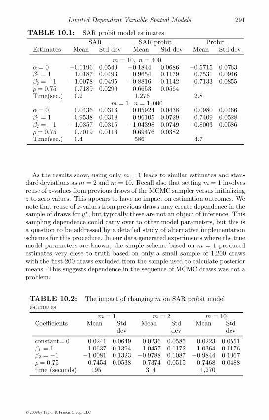
Limited Dependent Variable Spatial Models 291
TABLE 10.1: SAR probit model estimatesSAR SAR probit Probit
Estimates Mean Std dev Mean Std dev Mean Std dev
m = 10, n = 400α = 0 −0.1196 0.0549 −0.1844 0.0686 −0.5715 0.0763β1 = 1 1.0187 0.0493 0.9654 0.1179 0.7531 0.0946β2 = −1 −1.0078 0.0495 −0.8816 0.1142 −0.7133 0.0855ρ = 0.75 0.7189 0.0290 0.6653 0.0564Time(sec.) 0.2 1,276 2.8
m = 1, n = 1, 000α = 0 0.0436 0.0316 0.05924 0.0438 0.0980 0.0466β1 = 1 0.9538 0.0318 0.96105 0.0729 0.7409 0.0528β2 = −1 −1.0357 0.0315 −1.04398 0.0749 −0.8003 0.0586ρ = 0.75 0.7019 0.0116 0.69476 0.0382Time(sec.) 0.4 586 4.7
As the results show, using only m = 1 leads to similar estimates and stan-dard deviations as m = 2 and m = 10. Recall also that setting m = 1 involvesreuse of z-values from previous draws of the MCMC sampler versus initializingz to zero values. This appears to have no impact on estimation outcomes. Wenote that reuse of z-values from previous draws may create dependence in thesample of draws for y∗, but typically these are not an object of inference. Thissampling dependence could carry over to other model parameters, but this isa question to be addressed by a detailed study of alternative implementationschemes for this procedure. In our data generated experiments where the truemodel parameters are known, the simple scheme based on m = 1 producedestimates very close to truth based on only a small sample of 1,200 drawswith the first 200 draws excluded from the sample used to calculate posteriormeans. This suggests dependence in the sequence of MCMC draws was not aproblem.
TABLE 10.2: The impact of changing m on SAR probit modelestimates
m = 1 m = 2 m = 10Coefficients Mean Std Mean Std Mean Std
dev dev dev
constant= 0 0.0241 0.0649 0.0236 0.0585 0.0223 0.0551β1 = 1 1.0637 0.1394 1.0457 0.1172 1.0364 0.1176β2 = −1 −1.0081 0.1323 −0.9788 0.1087 −0.9844 0.1067ρ = 0.75 0.7454 0.0538 0.7374 0.0515 0.7468 0.0488time (seconds) 195 314 1,270
© 2009 by Taylor & Francis Group, LLC
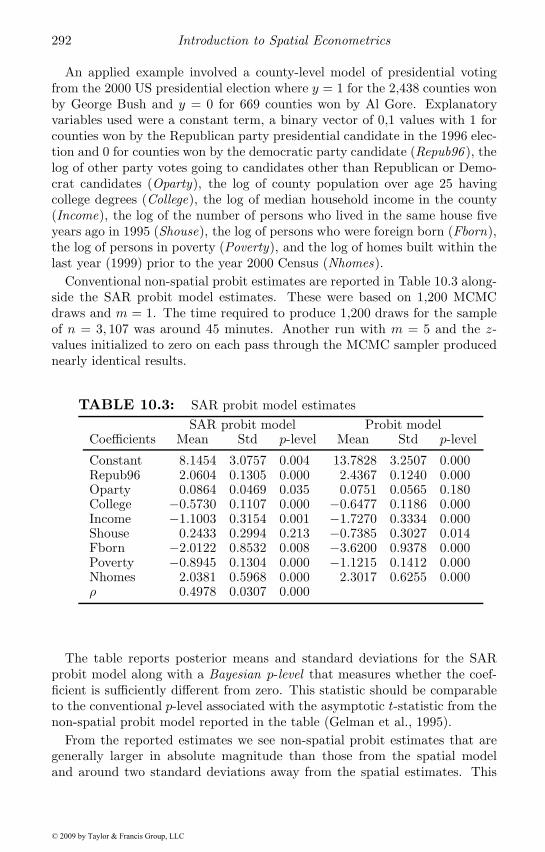
292 Introduction to Spatial Econometrics
An applied example involved a county-level model of presidential votingfrom the 2000 US presidential election where y = 1 for the 2,438 counties wonby George Bush and y = 0 for 669 counties won by Al Gore. Explanatoryvariables used were a constant term, a binary vector of 0,1 values with 1 forcounties won by the Republican party presidential candidate in the 1996 elec-tion and 0 for counties won by the democratic party candidate (Repub96 ), thelog of other party votes going to candidates other than Republican or Demo-crat candidates (Oparty), the log of county population over age 25 havingcollege degrees (College), the log of median household income in the county(Income), the log of the number of persons who lived in the same house fiveyears ago in 1995 (Shouse), the log of persons who were foreign born (Fborn),the log of persons in poverty (Poverty), and the log of homes built within thelast year (1999) prior to the year 2000 Census (Nhomes).
Conventional non-spatial probit estimates are reported in Table 10.3 along-side the SAR probit model estimates. These were based on 1,200 MCMCdraws and m = 1. The time required to produce 1,200 draws for the sampleof n = 3, 107 was around 45 minutes. Another run with m = 5 and the z-values initialized to zero on each pass through the MCMC sampler producednearly identical results.
TABLE 10.3: SAR probit model estimatesSAR probit model Probit model
Coefficients Mean Std p-level Mean Std p-level
Constant 8.1454 3.0757 0.004 13.7828 3.2507 0.000Repub96 2.0604 0.1305 0.000 2.4367 0.1240 0.000Oparty 0.0864 0.0469 0.035 0.0751 0.0565 0.180College −0.5730 0.1107 0.000 −0.6477 0.1186 0.000Income −1.1003 0.3154 0.001 −1.7270 0.3334 0.000Shouse 0.2433 0.2994 0.213 −0.7385 0.3027 0.014Fborn −2.0122 0.8532 0.008 −3.6200 0.9378 0.000Poverty −0.8945 0.1304 0.000 −1.1215 0.1412 0.000Nhomes 2.0381 0.5968 0.000 2.3017 0.6255 0.000ρ 0.4978 0.0307 0.000
The table reports posterior means and standard deviations for the SARprobit model along with a Bayesian p-level that measures whether the coef-ficient is sufficiently different from zero. This statistic should be comparableto the conventional p-level associated with the asymptotic t-statistic from thenon-spatial probit model reported in the table (Gelman et al., 1995).
From the reported estimates we see non-spatial probit estimates that aregenerally larger in absolute magnitude than those from the spatial modeland around two standard deviations away from the spatial estimates. This
© 2009 by Taylor & Francis Group, LLC
Limited Dependent Variable Spatial Models 293
is consistent with significant bias in the non-spatial estimates. There is oneinteresting reversal in sign associated with the Shouse variable, which is neg-ative and significant in the non-spatial model, but positive and not differentfrom zero in the spatial model. However, as in the case of continuous spatialregression models, we cannot directly compare these coefficient magnitudes.As is well-known for conventional probit models we need to evaluate the non-linear probit relationship by calculating marginal effects estimates. This isthe subject to which we turn attention in the next section.
10.1.6 Marginal effects for the spatial probit model
In non-spatial probit models, the parameter magnitudes associated withthe estimated coefficients β do not have the same marginal effects interpreta-tion as in standard regression models. This arises due to non-linearity in thenormal probability distribution. The magnitude of impact on the expectedprobability of the event y occurring varies with the level of say the rth ex-planatory variable, xr . The nature of this non-linear relationship betweenchanges in the dependent variable (the expected probability of the event) andchanges in xr is determined by the standard normal density such that:
∂E[y|xr]/∂xr = φ(xrβr)βr (10.9)
where βr is a non-spatial probit model estimate, and the expression φ(·) isthe standard normal density. Because the magnitude of impact on changesin expected probability varies with the level of xr, model estimates are ofteninterpreted using mean values of a regressor such as xr. The marginal effectsare then interpreted as the change in the event probability associated witha change in the average or typical sample observation for variable xr. Inaddition to the non-linear nature of the mean response of expected probabilityto changes in xr , there is also the need to consider a measure of dispersionfor this to provide a basis for statistical inference regarding the significanceof these changes.
In spatial regression models that involve spatial lags of the dependent vari-able (such as our SAR probit model), a change in the ith observation of the ex-planatory variable vector xir will impact the own region yi plus other-regionsyj , j �= i in the sample. This of course suggests that changes in the level of asingle observation xir will have an impact on the expected probability of theevent being analyzed in both own- and other-regions.
We have already established that E(∂y/∂x′r) = (In − ρW )−1Inβr for theSAR model, which is an n × n matrix. The diagonal of this matrix cap-tures what we have labeled the direct impact of a change in xir on the own-observation yi, with the off-diagonal elements representing indirect or spatialspillover impacts. This matrix replaces the non-spatial model coefficient βr,so we can calculate the marginal effects for our spatial SAR probit model by
© 2009 by Taylor & Francis Group, LLC
294 Introduction to Spatial Econometrics
replacing βr in (10.9) with this matrix. This leads to the expression in (10.10),where: S = (In − ρW ), and xr denotes the mean value of the rth variable.
∂E[y|xr]/∂x′r = φ(S−1Inxrβr) � S−1Inβr (10.10)
In place of the expression φ(xrβr) that scales the parameter estimate βrin the non-spatial probit model, we have a matrix, φ(S−1Inxrβr). And, inplace of the (scalar) coefficient βr from the non-spatial probit model, we haveanother matrix, S−1Inβr.
We can adopt the same approach taken earlier to develop scalar summarymeasures for the continuous dependent variable SAR model. The main di-agonal elements of φ
[(In − ρW )−1Inxrβr
]� (In − ρW )−1Inβr represent thedirect impacts, which we average over. Similarly, the average of the row (orcolumn) sums can be used to produce a total impact scalar summary mea-sure, and the indirect impacts are the difference between these two measures.We interpret the average of the row-sums as the average total impact fromchanging an observation, and the average of the column-sums as the averagetotal impact to an observation.
As an example, consider the decision to install a home security system,where the binary dependent variable indicates the absence (y = 0) or presence(y = 1) of security systems in a sample of n homes. Suppose we are interestedin the marginal effects of a variable xr recording the number of burglariesthat have occurred for each home in the sample. From the viewpoint of asingle homeowner i who is contemplating spending on an alarm system, theconventional probit model would indicate that a burglary at a neighboringhome j would have no effect on homeowner i’s decision to purchase a securitysystem. Only an increase in burglaries at home i represented by a change inxir would impact the probability that homeowner i makes a security systempurchase. The conventional use of the average or mean burglary rate xr tocalculate marginal effects has the implication that an increase in the meanburglary rate xr across the sample of homes would increase the probability ofall homeowners in the sample purchasing security systems. For this reason,the marginal effects are usually analyzed in the conventional model by varyingthe level of xr over the range of values taken by this variable to assess how thelevel of burglaries at various homes in the sample would impact the decisionto purchase a security system. Doing this creates a type of spatial variationin the effects estimates since the level of xr values vary over space.2 However,this does not imply any spatial interaction between observations, as this isnot possible in a non-spatial probit model.
In contrast, the SAR probit model implies that a change in burglaries ofneighboring homes j would have an effect on the probability that homeowneri purchases a security system. The effect would depend on spatial proximity
2This evaluation is of course conditional on all explanatory variables and associated coeffi-cient estimates) in the model, which are typically held fixed at their respective means.
© 2009 by Taylor & Francis Group, LLC
Limited Dependent Variable Spatial Models 295
of homeowner i to j, captured by the spatial weight matrix W , as well as thestrength of spatial dependence measured by the parameter ρ. A burglary athome j would have both a direct impact on the probability that homeowner jpurchases a security system, as well as an indirect or spatial spillover impacton neighbors. The total effect is the sum of these two impacts.
Conventional practice in the non-spatial probit model calculates marginaleffects using the point estimates (or posterior means in the case of Bayesiananalysis) and average variable values. One advantage of MCMC estimationis that the sample draws arising from estimation can be used to produceseparate marginal effects for every observation at each iteration (or using thesample of draws from the MCMC procedure in a post-estimation procedure).Averaging over these results recognizes the global nature of spatial spilloversthat cumulate across interrelated observations in the sample, and reflect thejoint posterior distribution of the model parameters.
Average marginal effects calculated in this fashion based on our scalar sum-mary measures of the direct and indirect impacts would produce impact es-timates that could be interpreted in the following way. The direct impactwould show how a rise in burglaries (burglaries on average across the sampleof homes) would affect the decision of (the average) individual homeowner be-ing burglarized to purchase a security system, where the impact is of coursemeasured in expected probability terms. The indirect effect would repre-sent the probabilistic impact of these increased burglaries on (the average)neighboring homeowners’ purchase decisions. We could of course carry outa partitioning of these impacts to determine the spatial extent of the effects,that is, the rate at which the impacts decay as we move to more distant neigh-bors. We further note that if interest centered on a sub-sample representinga particular neighborhood, these individual observations could be analyzed inthe same fashion.
In terms of the from an observation and to an observation interpretationfor our scalar summary measures of the impacts, we might consider the follow-ing interpretation. From a seller of security systems perspective, the modelestimates would be useful in determining to an observation impacts. Thesemeasure how changes in the mean burglaries would influence the probabilityof all homeowners in the sample purchasing systems (the total impact), whichwould be useful for projecting sales of security systems. In terms of the froman observation viewpoint, a security system salesperson could use the modelestimates to determine how likely individual homeowners who have been bur-glarized (the direct impact) and their neighbors (the indirect impact) are topurchase a system.
In addition to calculating mean summary measures for the spatial marginaleffects, there is also a need to calculate measures of dispersion for these es-timates. This could be done using the MCMC draws in expression (10.10)to construct a posterior distribution for the spatial marginal effects summarymeasures. A computationally efficient approach to doing this remains a sub-ject for future research.
© 2009 by Taylor & Francis Group, LLC
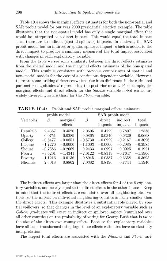
296 Introduction to Spatial Econometrics
Table 10.4 shows the marginal effects estimates for both the non-spatial andSAR probit model for our year 2000 presidential election example. The tableillustrates that the non-spatial model has only a single marginal effect thatwould be interpreted as a direct impact. This would equal the total impactsince there are no indirect (spatial spillover) impacts. In contrast, the SARprobit model has an indirect or spatial spillover impact, which is added to thedirect impact to produce a summary measure of the total impact associatedwith changes in each explanatory variable.
From the table we see some similarity between the direct effects estimatesfrom the spatial model and the marginal effects estimates of the non-spatialmodel. This result is consistent with previous comparisons of spatial andnon-spatial models for the case of a continuous dependent variable. However,there are some striking differences which arise from differences in the estimatedparameter magnitudes β representing the posterior means. For example, themarginal effects and direct effects for the Shouse variable noted earlier arewidely divergent, as are those for the Fborn variable.
TABLE 10.4: Probit and SAR probit marginal effects estimatesprobit model SAR probit model
Variables β marginal β direct indirect totaleffects impacts impacts impacts
Repub96 2.4367 0.4520 2.0605 0.4729 0.7807 1.2536Oparty 0.0751 0.0289 0.0865 0.0340 0.0329 0.0668College −0.6477 −0.0851 −0.5730 −0.0929 −0.2167 −0.3096Income −1.7270 −0.0000 −1.1003 −0.0000 −0.2985 −0.2985Shouse −0.7386 −0.2669 0.2433 0.0997 0.0925 0.1921Fborn −3.6201 −1.4341 −2.0122 −0.8319 −0.7647 −1.5966Poverty −1.1216 −0.0136 −0.8945 −0.0337 −0.3358 −0.3695Nhomes 2.3018 0.8862 2.0382 0.8196 0.7744 1.5940
The indirect effects are larger than the direct effects for 4 of the 8 explana-tory variables, and nearly equal to the direct effects in the other 4 cases. Keepin mind that the indirect effects are cumulated over all neighboring observa-tions, so the impact on individual neighboring counties is likely smaller thanthe direct effects. This example illustrates a substantial role played by spa-tial spillovers, so that changes in the level of an explanatory variable such asCollege graduates will exert an indirect or spillover impact (cumulated overall other counties) on the probability of voting for George Bush that is twicethe size of the direct own-county effect. Because the explanatory variableshave all been transformed using logs, these effects estimates have an elasticityinterpretation.
The largest total effects are associated with the Nhomes and Fborn vari-
© 2009 by Taylor & Francis Group, LLC
Limited Dependent Variable Spatial Models 297
ables, having elasticities around 1.6 and −1.6 respectively. The binary variableRepub96 representing a win by the 1996 Republican party presidential can-didate is also large, but does not have the same elasticity interpretation asother explanatory variables. Votes for candidates such as Nader or Buchanan(Oparty) had positive direct and indirect impacts around 0.033 leading to atotal effect around 0.066. This suggests that a 10 percent increase in thesevotes increased the probability of Bush winning the county by around 2/3of one percent. We note that the coefficient estimate for this variable is notsignificantly different from zero in the conventional probit model, but has aBayesian p-level of 0.035, suggesting a non-zero impact. To further explorethe importance of other party candidates on the probability of Bush winninga county, one would need to calculate a measure of dispersion for the meaneffects estimates reported in the table.
10.2 The ordered spatial probit model
One extension to the spatial probit model is an ordered probit model. Thistype of model describes a situation where we can observe more than twochoice outcomes, but the alternatives must take a particular form. Theymust be ordered, which may arise in certain modeling situations where thealternatives exhibit a natural or logical ordering. For example, if we hadsurvey information where participants are asked to choose from alternativessuch as: Strongly Agree, Agree, Uncertain, Disagree, Strongly Disagree, thenthe choice set exhibits a natural ordering.
The ordered spatial probit model would generalize the basic model fromSection 10.1, but still rely on the relationship between y∗ and y. If the ob-served choice outcomes yi can take ordered values {j = 1, . . . , J}, where J isthe number of ordered alternatives, then we posit the relationship in (10.11),
yi = j, if φj−1 < y∗i ≤ φj (10.11)
where φ0 ≤ φ1 ≤ . . . ≤ φJ are parameters to be estimated. The probitmodel we already examined is a special case of this model where J = 2 andφ0 = −∞, φ1 = 0, and φ2 = +∞. This turns out to be an identificationrestriction that is typically placed on the ordered probit model, where therestriction for a J alternative model takes the form: φ0 = −∞, φ1 = 0, andφJ = +∞. The other φj , j = 2, . . . , J − 1 are parameters to be estimated.
The parameters φj , j = 2, . . . , J − 1 can be added to a Bayesian MCMCestimation scheme by sampling from their conditional posterior distributions.In the non-spatial model, Koop (2003) shows that the form of the conditionalposterior can be deduced for the case of a flat or uniform prior by arguing:
© 2009 by Taylor & Francis Group, LLC
298 Introduction to Spatial Econometrics
1. Conditional on knowing the other parameters which we denote φ−j , weknow that φj must lie in the interval [φj−1, φj+1].
2. Conditional on both y∗, y we know which values of the latent data y∗
correspond to the observed choices y, the insight of Albert and Chib(1993).
3. The conditional posterior distribution for the parameters φ is based onno other information from the model.
Items 1) to 3) above imply a uniform conditional posterior distribution forφj , j = 2, . . . , J − 1 taking the form:
p(φj |φ−j , y∗, y, β) ∼ U(φj−1, φj+1), j = 2, . . . , J − 1 (10.12)
The bounding or cut-point values φ are determined by examining the max-imum (and minimum) values of the latent data y∗i over all individuals i whohave chosen alternative j, that is where yi = j. Since individuals’ choicesare independent from those of other individuals in the non-spatial model, thisleads to:
φj−1 = max{max{y∗i : yi = j}, φj−1}φj+1 = min{min{y∗i : yi = j + 1}, φj+1}
For the case of our ordered spatial probit model we do not have indepen-dence between choices of individuals, so we need to consider if this sameapproach can be applied. In Section 10.6 we discuss a space-time dynamicordered probit model introduced by Wang and Kockelman (2008a,b) that al-lows for spatially structured random effects. In their model where individualchoices are dependent across both time and space, the cut-points exhibit de-pendence invalidating the non-spatial approach.
In our cross-sectional model, we can sample from the conditional distribu-tion for each y∗i , making these unconditional on other y∗j . This allows us touse an argument that there is conditional independence in the sampled y∗i ,and apply the same approach to sampling the cut-points φj−1 and φj+1. Thisinvolves making a claim that for all i:
max{max{y∗i |z(m) : yi = j}, φj−1} = max{max{y∗i : yi = j}, φj−1}min{min{y∗i |z(m) : yi = j}, φj+1} = min{min{y∗i : yi = j}, φj+1}
where the equality arises from using the Gibbs sampler to produce a distribu-tion for the vector y∗ using zi|z−i that takes spatial dependence into account.If this argument is plausible, then we can resort to an m-step Gibbs sampler:
© 2009 by Taylor & Francis Group, LLC
Limited Dependent Variable Spatial Models 299
zi|z−i = γ−iz−i + hivi (10.13)hi = (Ψi,i)−1/2
where we sample vi ∼ N(0, 1) and use the truncation constraints:
(b1 − γ−iz−i)/hi < vi ≤ (b1 − γ−iz−i)/hi, for yi = 1
(b2 − γ−iz−i)/hi < vi ≤ (b2 − γ−iz−i)/hi, for yi = 2...
(bJ − γ−iz−i)/hi < vi ≤ (bJ − γ−iz−i)/hi, for yi = J
Where:
b1 = −∞ and b1 = 0 for yi = 1b2 = 0 and b2 = φ2 for yi = 2
...bJ = φJ−1 and bJ = +∞ for yi = J
(10.14)
Given these assumptions, this model and associated MCMC procedure rep-resents a relatively simple extension of the spatial probit model. After mak-ing a series of m passes through the n-observation vector z, we generatey∗ = μ + z(m). The vector y∗ can then be used to produce draws from theconditional distributions for the remaining model parameters β, ρ, φ as in thebinary spatial probit model.
10.3 Spatial Tobit models
These models deal with situations where a subset of the observations arebelieved to represent censored values, which result in a truncated distributionfor the dependent variable observations. We might argue that censoring ofsome sample observations arose because the utility is negative for an actionmeasured by our dependent variable observations y. For example, if y mea-sures the number of persons in a sample of census tracts who commute towork by walking, there may be a number of zero observations. These couldbe argued to represent census tracts where the utility associated with walkingas a mode of travel to work is negative.
This same line of argument was used to motivate the truncated multivariatenormal conditional posterior distributions for the latent unobserved utilities
© 2009 by Taylor & Francis Group, LLC
300 Introduction to Spatial Econometrics
in the case of spatial probit. Indeed the same approach as taken by Albertand Chib (1993) works here, as was pointed out by Chib (1992) for the caseof non-spatial Tobit models. In terms of motivation for spatial dependence incensored observations, it seems likely that census tracts located nearby in largecities would have similar numbers of persons who walk to work. It should alsobe clear that large rural census tracts, or those in outlying suburbs are notlikely to see commuters walking to work as the utility is probably negative.Another example used earlier is the case of regional trade flows, where wemight expect to see zero flows between regions where the trade costs exceed athreshold level. Since trade costs are thought to be related to distance, zerotrade flows between origin and destination regions might imply zero flowsfor neighbors to the origin to the same destination, and vice versa. Similarsituations arise in observed and unobserved home selling prices. There may bea number of homes that do not sell because the utility associated with owninga house in a central city location plagued by crime and negative externalitiesfrom neighboring homes that are abandoned or in poor condition might bebelow a threshold level required to undertake the transaction costs.
The latent regression model motivation for this model when censoring oc-curs at zero takes the form in (10.15), where y2 denotes a vector of non-censored observations.
y∗ = S−1Xβ + S−1ε (10.15)y∗ = y∗1 if y∗ ≤ 0y∗ = y2 otherwiseS = In − ρW
For the case of Tobit, where we have a block of n1 censored observations andanother set of n2 observed values, we need only produce latent y∗1 for the n1
censored observations. We construct the mean and variance-covariance matrixfor the block of n1 censored observations conditional on the n2 uncensoredobservations y2. We assume the locations of all observations are known, so then×n weight matrix W can be formed. The conditional posterior distributionfor the n1 censored observations can be expressed as a multivariate truncatednormal distribution y∗1 ∼ TMVN(μ∗
1,Ω∗1,1), where the mean and variance-
covariance are set forth in (10.16) and (10.17).
© 2009 by Taylor & Francis Group, LLC
Limited Dependent Variable Spatial Models 301
μ∗1 = E(y∗1 |y2, X,W, β, ρ, σ2
ε)= μ1 − (Ψ1,1)−1Ψ1,2(y2 − μ2) (10.16)
Ω∗1,1 = var-cov(y∗1 |y2, X,W, β, ρ, σ2
ε)
= Ω1,1 + (Ψ1,1)−1Ψ1,2Ω2,1 (10.17)Ω = σ2
ε [(In − ρW )′(In − ρW )]−1
Ψ = Ω−1
μ1 = (In − ρW )−11,1X1β
μ2 = (In − ρW )−12,2X2β
We use the subscripts 1, 2 to denote an n1×n2 matrix, and matrices such asΩ1,1 would contain n1 rows and columns, whereas Ω2,2 would be of dimensionn2 × n2. The term (In − ρW )−1
1,1 refers to the n1 × n1 block of the matrixinverse (In−ρW )−1, and a similar definition applies to the n2×n2 block usedin μ2. Note that we have a scalar noise variance parameter σ2
ε in the model,which appears in the expressions for Ω and Ψ.
Fortunately, calculating Ω = Ψ−1 is not necessary. This would be requiredon each pass through the MCMC sampler because the parameters ρ and σ2
ε
change, making estimation of this model computationally challenging. TheGeweke m-step Gibbs sampler used to produce draws from the multivariatetruncated normal distribution works with the precison matrix Ψ = Ω−1. Wecan calculate the matrices W +W ′ and W ′W prior to beginning the MCMCsampling loop and produce Ψ = (1/σ2
ε)[In − ρ(W +W ′) + ρ2W ′W ] using thecurrent values of ρ and σ2
ε obtained during sampling. The terms needed toform the n1-dimensional mean and variance-covariance for the the block of n1
TMVN censored observations are:
μ∗1 = μ1 − (Ψ1,1)−1Ψ1,2(y2 − μ2)
Ψ∗11 = (In1 − ρ(W +W ′)1,1 + ρ2(W ′W )1,1)/σ2
ε
where (W +W ′)1,1 and (W ′W )1,1 refer to the block of n1 × n1 observationstaken from the matrices (W +W ′) and (W ′W ).
Given the n1×1 vector μ∗1 of means and associated precision matrix Ψ∗
11, weuse the Geweke m-step Gibbs sampling procedure to carry out a sequence ofm draws for each censored observation i = 1, . . . , n1 conditional on all othercensored observations which we label −i. Of course, we follow the schemedetailed in our discussion of the spatial probit model, where previously sam-pled censored observation values are used when sampling the ith observationduring each pass through the Gibbs sampler. This can be used to build upthe joint conditional multivariate posterior distribution for the n1 × 1 latentvector y∗1 which is used to replace the censored observations. Specifically, we
© 2009 by Taylor & Francis Group, LLC
302 Introduction to Spatial Econometrics
generate y∗1 = μ∗1 +z(m), where m denotes the number of passes made and the
vector z is for censored observations. These are sampled from the completesequence of univariate (conditional) distributions, zi|z−i.
This procedure represents a Gibbs sampling scheme that takes into accountdependence between observed and unobserved observations when calculatingμ∗
1 and Ω∗1,1, and then uses the m-step Gibbs sampler to build up the joint dis-
tribution for the n1×1 vector z of censored observations. This latter proceduretakes into account spatial dependence between the censored observations.
These latent parameters are then used to produce a full-sample of observa-tions y∗ =
(y∗
′1 y′2
)′, some of which are observed values and others represent
sampled unobserved latent variables. The full-sample vector y∗ is then usedwhen sampling from the conditional posterior distributions for the remainingmodel parameters β, ρ, σ2
ε .For the standard non-spatial tobit model with censoring at zero and nor-
mally distributed disturbances the marginal effects for the censored regressionmodel take the form, Greene (2000).
∂E[yi|xr]/∂xr = βΦ (x′rβ/σ) (10.18)
where Φ(·) represents the normal CDF function and the subscript r referencesa variable. Intuitively, this expression indicates that the maximum likelihoodTobit coefficient estimates are adjusted versions of least-squares estimates,where the adjustment involves the proportion of the sample that is censored.
We have already explored expressions like ∂E[y|xr]/∂x′r for our SAR modelin the context of interpreting the parameter estimates, as well as calculatingSAR probit marginal effects. A similar approach can be used here where themissing or censored observations are replaced with the posterior mean of thedraws for the latent values y∗1 .
10.3.1 An example of the spatial Tobit model
A data-generated experiment from Koop (2003), which allows us to controlthe degree of sample censoring was adapted to generate a sample of 1,000 ob-servations. We draw independent observations xi from a uniform distribution,U(a, 1) and a disturbance term εi ∼ N(0, 0.5). These are used to construct:
y∗ = (In − ρW )−1Xβ + (In − ρW )−1ε (10.19)
A value of ρ = 0.7 was used in conjunction with a spatial weight matrixW generated using random locational coordinates and six nearest neighbors.The degree of censoring that occurs can be controlled using different settingsfor the parameter a. Negative generated values from the vector y∗ are set tozero to reflect sample truncation at zero. We report results for an experimentwhere 51.3 percent of the 1,000 observation sample was censored.
These are shown in Table 10.5 where we also report Bayesian MCMC SARmodel estimates based on the true non-censored values. Ideally, we would like
© 2009 by Taylor & Francis Group, LLC
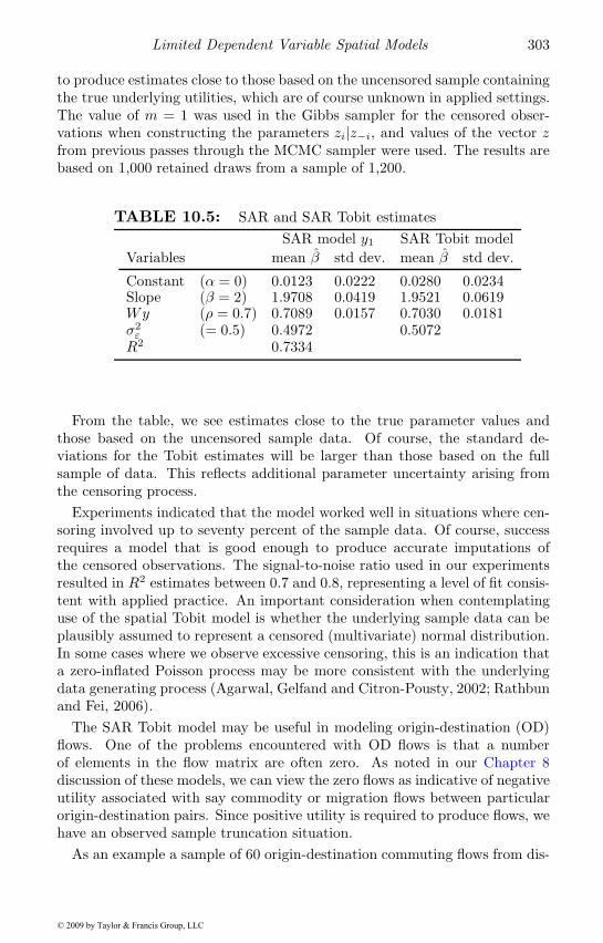
Limited Dependent Variable Spatial Models 303
to produce estimates close to those based on the uncensored sample containingthe true underlying utilities, which are of course unknown in applied settings.The value of m = 1 was used in the Gibbs sampler for the censored obser-vations when constructing the parameters zi|z−i, and values of the vector zfrom previous passes through the MCMC sampler were used. The results arebased on 1,000 retained draws from a sample of 1,200.
TABLE 10.5: SAR and SAR Tobit estimatesSAR model y1 SAR Tobit model
Variables mean β std dev. mean β std dev.
Constant (α = 0) 0.0123 0.0222 0.0280 0.0234Slope (β = 2) 1.9708 0.0419 1.9521 0.0619Wy (ρ = 0.7) 0.7089 0.0157 0.7030 0.0181σ2ε (= 0.5) 0.4972 0.5072R2 0.7334
From the table, we see estimates close to the true parameter values andthose based on the uncensored sample data. Of course, the standard de-viations for the Tobit estimates will be larger than those based on the fullsample of data. This reflects additional parameter uncertainty arising fromthe censoring process.
Experiments indicated that the model worked well in situations where cen-soring involved up to seventy percent of the sample data. Of course, successrequires a model that is good enough to produce accurate imputations ofthe censored observations. The signal-to-noise ratio used in our experimentsresulted in R2 estimates between 0.7 and 0.8, representing a level of fit consis-tent with applied practice. An important consideration when contemplatinguse of the spatial Tobit model is whether the underlying sample data can beplausibly assumed to represent a censored (multivariate) normal distribution.In some cases where we observe excessive censoring, this is an indication thata zero-inflated Poisson process may be more consistent with the underlyingdata generating process (Agarwal, Gelfand and Citron-Pousty, 2002; Rathbunand Fei, 2006).
The SAR Tobit model may be useful in modeling origin-destination (OD)flows. One of the problems encountered with OD flows is that a numberof elements in the flow matrix are often zero. As noted in our Chapter 8discussion of these models, we can view the zero flows as indicative of negativeutility associated with say commodity or migration flows between particularorigin-destination pairs. Since positive utility is required to produce flows, wehave an observed sample truncation situation.
As an example a sample of 60 origin-destination commuting flows from dis-
© 2009 by Taylor & Francis Group, LLC
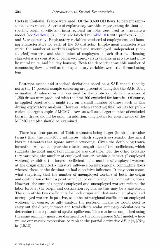
304 Introduction to Spatial Econometrics
tricts in Toulouse, France were used. Of the 3,600 OD flows 15 percent repre-sented zero values. A series of explanatory variables representing destination-specific, origin-specific and intra-regional variables were used to formulate amodel (see Section 8.3). These are labeled in Table 10.6 with prefixes D ,Oand I respectively. Explanatory variables consisted of employment and hous-ing characteristics for each of the 60 districts. Employment characteristicswere: the number of workers employed and unemployed, independent (non-salaried) workers, and the number of employers in each district. Housingcharacteristics consisted of owner-occupied versus tenants in private and pub-lic rental units, and holiday housing. Both the dependent variable number ofcommuting flows as well as the explanatory variables were transformed usinglogs.
Posterior means and standard deviations based on a SAR model that ig-nores the 15 percent sample censoring are presented alongside the SAR Tobitestimates. A value of m = 1 was used for the Gibbs sampler and a series of1,200 draws were produced with the first 200 excluded for burn-in. Of course,in applied practice one might rely on a small number of draws such as thisduring exploratory analysis. However, when reporting final results for publi-cation, a larger sample of MCMC draws as well as a larger number of excludedburn-in draws should be used. In addition, diagnostics for convergence of theMCMC sampler should be examined.
There is a clear pattern of Tobit estimates being larger (in absolute valueterms) than the non-Tobit estimates, which suggests systematic downwardbias in estimates that ignore sample censoring. Given the double-log trans-formation, we can compare the relative magnitudes of the coefficients, whichsuggests the most important influence was distance. For the other explana-tory variables, the number of employed workers within a district (I employedworkers) exhibited the largest coefficient. The number of employed workersat the origin exhibited a negative influence on interregional commuting flowswhereas those at the destination had a positive influence. It may seem some-what surprising that the number of unemployed workers at both the originand destination exhibit a positive influence on interregional commuting flows.However, the sum of (logged) employed and unemployed workers reflects thelabor force at the origin and destination regions, so this may be a size effect.The sum of the two coefficients for both origin and destination employed andunemployed workers is positive, as is the intraregional coefficient on employedworkers. Of course, to fully analyze the posterior means we would need tocarry out the direct, indirect and total effects scalar summary calculations todetermine the magnitude of spatial spillovers. This can be accomplished usingthe same summary measures discussed for the non-censored SAR model, wherewe use our matrix expressions to replace the partial derivative ∂E[yi|xr]/∂xrin (10.18).
© 2009 by Taylor & Francis Group, LLC
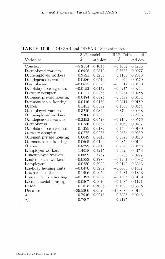
Limited Dependent Variable Spatial Models 305
TABLE 10.6: OD SAR and OD SAR Tobit estimatesSAR model SAR Tobit model
Variables β std dev. β std dev.
Constant −5.2154 0.4044 −6.1607 0.4705D employed workers 0.6928 0.0812 0.7635 0.0977D unemployed workers 0.9521 0.2206 1.1150 0.2623D independent workers 0.0586 0.0516 0.0946 0.0579D employers −0.0675 0.0373 −0.0817 0.0430D holiday housing units −0.0192 0.0172 −0.0275 0.0204D owner occupier 0.0121 0.0236 0.0261 0.0288D tenant private housing −0.0484 0.0384 −0.0438 0.0474D tenant social housing −0.0416 0.0160 −0.0311 0.0189D area 0.1451 0.0382 0.1368 0.0484O employed workers −0.3210 0.0824 −0.3790 0.0948O unemployed workers 1.2306 0.2335 1.5633 0.2556O independent workers −0.2392 0.0528 −0.2162 0.0576O employers −0.0786 0.0362 −0.1053 0.0407O holiday housing units 0.1325 0.0182 0.1469 0.0180O owner occupier −0.0772 0.0238 −0.0854 0.0259O tenant private housing 0.6049 0.0415 0.6873 0.0423O tenant social housing −0.0665 0.0162 −0.0859 0.0194O area 0.8222 0.0418 0.9543 0.0448I employed workers 1.4038 0.3215 1.6420 0.3758I unemployed workers 0.6099 1.7787 1.0200 2.0277I independent workers −0.0833 0.3789 −0.1261 0.4082I employers 0.0250 0.2903 0.0149 0.3313I holiday housing units −0.0470 0.1262 −0.0680 0.1467I owner occupier −0.1996 0.1659 −0.2281 0.1893I tenant private housing −0.1393 0.2839 −0.1584 0.3109I tenant social housing −0.0907 0.1020 −0.1386 0.1121I area 0.1625 0.3006 0.1900 0.3308Distance −39.5906 6.6526 −47.8385 8.0114ρ 0.7646 0.0215 0.7328 0.0215σ2ε 0.7007 0.9125
© 2009 by Taylor & Francis Group, LLC
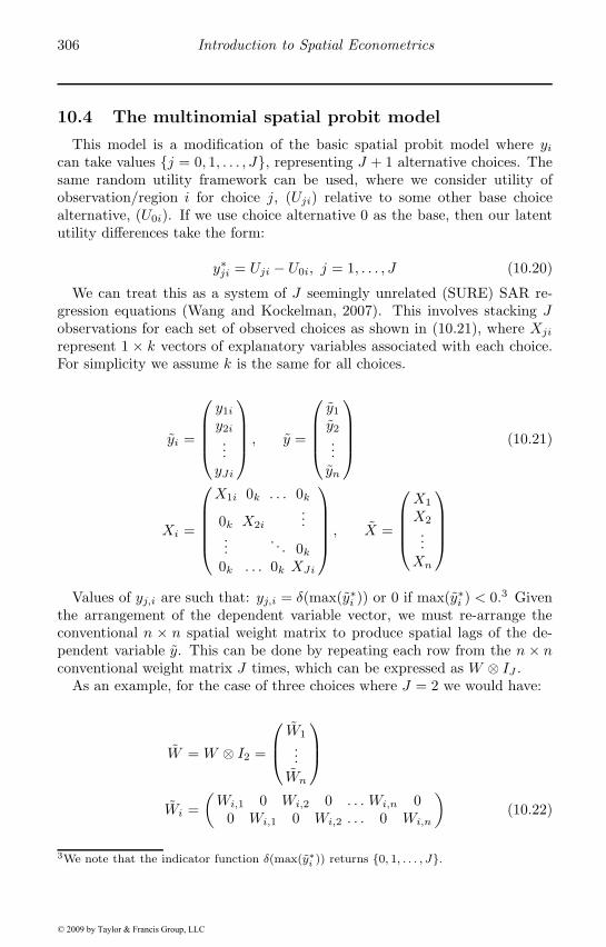
306 Introduction to Spatial Econometrics
10.4 The multinomial spatial probit model
This model is a modification of the basic spatial probit model where yican take values {j = 0, 1, . . . , J}, representing J + 1 alternative choices. Thesame random utility framework can be used, where we consider utility ofobservation/region i for choice j, (Uji) relative to some other base choicealternative, (U0i). If we use choice alternative 0 as the base, then our latentutility differences take the form:
y∗ji = Uji − U0i, j = 1, . . . , J (10.20)
We can treat this as a system of J seemingly unrelated (SURE) SAR re-gression equations (Wang and Kockelman, 2007). This involves stacking Jobservations for each set of observed choices as shown in (10.21), where Xji
represent 1 × k vectors of explanatory variables associated with each choice.For simplicity we assume k is the same for all choices.
yi =
⎛⎜⎜⎜⎝y1iy2i...yJi
⎞⎟⎟⎟⎠ , y =
⎛⎜⎜⎜⎝y1y2...yn
⎞⎟⎟⎟⎠ (10.21)
Xi =
⎛⎜⎜⎜⎜⎝X1i 0k . . . 0k
0k X2i
......
. . . 0k0k . . . 0k XJi
⎞⎟⎟⎟⎟⎠ , X =
⎛⎜⎜⎜⎝X1
X2
...Xn
⎞⎟⎟⎟⎠Values of yj,i are such that: yj,i = δ(max(y∗i )) or 0 if max(y∗i ) < 0.3 Given
the arrangement of the dependent variable vector, we must re-arrange theconventional n × n spatial weight matrix to produce spatial lags of the de-pendent variable y. This can be done by repeating each row from the n × nconventional weight matrix J times, which can be expressed as W ⊗ IJ .
As an example, for the case of three choices where J = 2 we would have:
W = W ⊗ I2 =
⎛⎜⎝ W1
...Wn
⎞⎟⎠Wi =
(Wi,1 0 Wi,2 0 . . . Wi,n 0
0 Wi,1 0 Wi,2 . . . 0 Wi,n
)(10.22)
3We note that the indicator function δ(max(y∗i )) returns {0, 1, . . . , J}.
© 2009 by Taylor & Francis Group, LLC
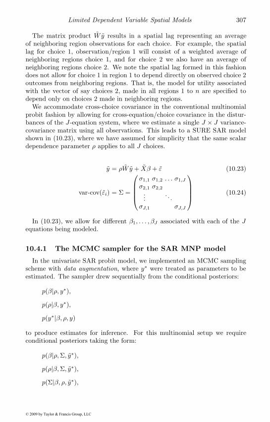
Limited Dependent Variable Spatial Models 307
The matrix product W y results in a spatial lag representing an averageof neighboring region observations for each choice. For example, the spatiallag for choice 1, observation/region 1 will consist of a weighted average ofneighboring regions choice 1, and for choice 2 we also have an average ofneighboring regions choice 2. We note the spatial lag formed in this fashiondoes not allow for choice 1 in region 1 to depend directly on observed choice 2outcomes from neighboring regions. That is, the model for utility associatedwith the vector of say choices 2, made in all regions 1 to n are specified todepend only on choices 2 made in neighboring regions.
We accommodate cross-choice covariance in the conventional multinomialprobit fashion by allowing for cross-equation/choice covariance in the distur-bances of the J-equation system, where we estimate a single J × J variance-covariance matrix using all observations. This leads to a SURE SAR modelshown in (10.23), where we have assumed for simplicity that the same scalardependence parameter ρ applies to all J choices.
y = ρW y + Xβ + ε (10.23)
var-cov(εi) = Σ =
⎛⎜⎜⎜⎝σ1,1 σ1,2 . . . σ1,J
σ2,1 σ2,2
.... . .
σJ,1 σJ,J
⎞⎟⎟⎟⎠ (10.24)
In (10.23), we allow for different β1, . . . , βJ associated with each of the Jequations being modeled.
10.4.1 The MCMC sampler for the SAR MNP model
In the univariate SAR probit model, we implemented an MCMC samplingscheme with data augmentation, where y∗ were treated as parameters to beestimated. The sampler drew sequentially from the conditional posteriors:
p(β|ρ, y∗),p(ρ|β, y∗),p(y∗|β, ρ, y)
to produce estimates for inference. For this multinomial setup we requireconditional posteriors taking the form:
p(β|ρ,Σ, y∗),p(ρ|β,Σ, y∗),p(Σ|β, ρ, y∗),
© 2009 by Taylor & Francis Group, LLC
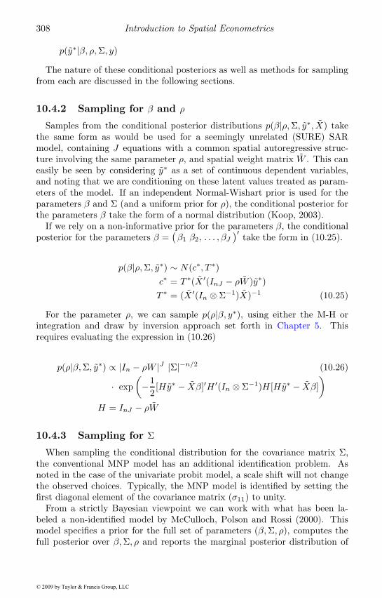
308 Introduction to Spatial Econometrics
p(y∗|β, ρ,Σ, y)The nature of these conditional posteriors as well as methods for sampling
from each are discussed in the following sections.
10.4.2 Sampling for β and ρ
Samples from the conditional posterior distributions p(β|ρ,Σ, y∗, X) takethe same form as would be used for a seemingly unrelated (SURE) SARmodel, containing J equations with a common spatial autoregressive struc-ture involving the same parameter ρ, and spatial weight matrix W . This caneasily be seen by considering y∗ as a set of continuous dependent variables,and noting that we are conditioning on these latent values treated as param-eters of the model. If an independent Normal-Wishart prior is used for theparameters β and Σ (and a uniform prior for ρ), the conditional posterior forthe parameters β take the form of a normal distribution (Koop, 2003).
If we rely on a non-informative prior for the parameters β, the conditionalposterior for the parameters β =
(β1 β2, . . . , βJ
)′ take the form in (10.25).
p(β|ρ,Σ, y∗) ∼ N(c∗, T ∗)c∗ = T ∗(X ′(InJ − ρW )y∗)T ∗ = (X ′(In ⊗ Σ−1)X)−1 (10.25)
For the parameter ρ, we can sample p(ρ|β, y∗), using either the M-H orintegration and draw by inversion approach set forth in Chapter 5. Thisrequires evaluating the expression in (10.26)
p(ρ|β,Σ, y∗) ∝ |In − ρW |J |Σ|−n/2 (10.26)
· exp(−1
2[Hy∗ − Xβ]′H ′(In ⊗ Σ−1)H [Hy∗ − Xβ]
)H = InJ − ρW
10.4.3 Sampling for Σ
When sampling the conditional distribution for the covariance matrix Σ,the conventional MNP model has an additional identification problem. Asnoted in the case of the univariate probit model, a scale shift will not changethe observed choices. Typically, the MNP model is identified by setting thefirst diagonal element of the covariance matrix (σ11) to unity.
From a strictly Bayesian viewpoint we can work with what has been la-beled a non-identified model by McCulloch, Polson and Rossi (2000). Thismodel specifies a prior for the full set of parameters (β,Σ, ρ), computes thefull posterior over β,Σ, ρ and reports the marginal posterior distribution of
© 2009 by Taylor & Francis Group, LLC
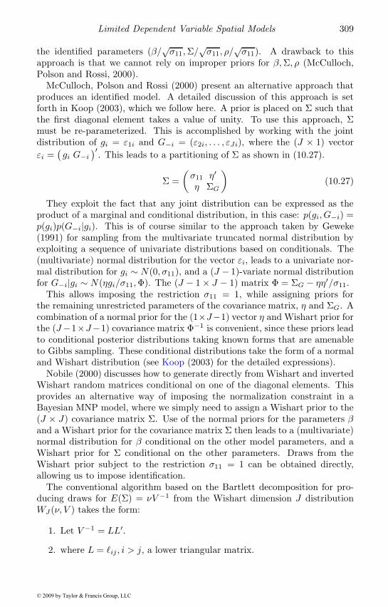
Limited Dependent Variable Spatial Models 309
the identified parameters (β/√σ11,Σ/
√σ11, ρ/
√σ11). A drawback to this
approach is that we cannot rely on improper priors for β,Σ, ρ (McCulloch,Polson and Rossi, 2000).
McCulloch, Polson and Rossi (2000) present an alternative approach thatproduces an identified model. A detailed discussion of this approach is setforth in Koop (2003), which we follow here. A prior is placed on Σ such thatthe first diagonal element takes a value of unity. To use this approach, Σmust be re-parameterized. This is accomplished by working with the jointdistribution of gi = ε1i and G−i = (ε2i, . . . , εJi), where the (J × 1) vectorεi =
(gi G−i
)′. This leads to a partitioning of Σ as shown in (10.27).
Σ =(σ11 η′
η ΣG
)(10.27)
They exploit the fact that any joint distribution can be expressed as theproduct of a marginal and conditional distribution, in this case: p(gi, G−i) =p(gi)p(G−i|gi). This is of course similar to the approach taken by Geweke(1991) for sampling from the multivariate truncated normal distribution byexploiting a sequence of univariate distributions based on conditionals. The(multivariate) normal distribution for the vector εi, leads to a univariate nor-mal distribution for gi ∼ N(0, σ11), and a (J − 1)-variate normal distributionfor G−i|gi ∼ N(ηgi/σ11,Φ). The (J − 1 × J − 1) matrix Φ = ΣG − ηη′/σ11.
This allows imposing the restriction σ11 = 1, while assigning priors forthe remaining unrestricted parameters of the covariance matrix, η and ΣG. Acombination of a normal prior for the (1×J−1) vector η and Wishart prior forthe (J−1×J−1) covariance matrix Φ−1 is convenient, since these priors leadto conditional posterior distributions taking known forms that are amenableto Gibbs sampling. These conditional distributions take the form of a normaland Wishart distribution (see Koop (2003) for the detailed expressions).
Nobile (2000) discusses how to generate directly from Wishart and invertedWishart random matrices conditional on one of the diagonal elements. Thisprovides an alternative way of imposing the normalization constraint in aBayesian MNP model, where we simply need to assign a Wishart prior to the(J × J) covariance matrix Σ. Use of the normal priors for the parameters βand a Wishart prior for the covariance matrix Σ then leads to a (multivariate)normal distribution for β conditional on the other model parameters, and aWishart prior for Σ conditional on the other parameters. Draws from theWishart prior subject to the restriction σ11 = 1 can be obtained directly,allowing us to impose identification.
The conventional algorithm based on the Bartlett decomposition for pro-ducing draws for E(Σ) = νV −1 from the Wishart dimension J distributionWJ (ν, V ) takes the form:
1. Let V −1 = LL′.
2. where L = �ij , i > j, a lower triangular matrix.
© 2009 by Taylor & Francis Group, LLC
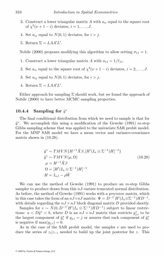
310 Introduction to Spatial Econometrics
3. Construct a lower triangular matrix A with aii equal to the square rootof χ2(ν + 1 − i) deviates, i = 1, . . . , J .
4. Set aij equal to N(0, 1) deviates, for i > j.
5. Return Σ = LAA′L′.
Nobile (2000) proposes modifying this algorithm to allow setting σ11 = 1.
1. Construct a lower triangular matrix A with a11 = 1/�11.
2. Set aii equal to the square root of χ2(ν + 1 − i) deviates, i = 2, . . . , J .
3. Set aij equal to N(0, 1) deviates, for i > j.
4. Return Σ = LAA′L′.
Either approach for sampling Σ should work, but we found the approach ofNobile (2000) to have better MCMC sampling properties.
10.4.4 Sampling for y∗
The final conditional distribution from which we need to sample is that fory∗. We accomplish this using a modification of the Geweke (1991) m-stepGibbs sampling scheme that was applied to the univariate SAR probit model.For the MNP SAR model we have a mean vector and variance-covariancematrix shown in (10.28).
y∗ ∼ TMVN{H−1Xβ, [H ′(In ⊗ Σ−1)H ]−1}y∗ ∼ TMVN(μ,Ω) (10.28)μ = H−1Xβ
Ω = [H ′(In ⊗ Σ−1)H ]−1
H = InJ − ρW
We can use the method of Geweke (1991) to produce an m-step Gibbssampler to produce draws from this nJ-variate truncated normal distribution.As before, the method of Geweke (1991) works with a precision matrix, whichin this case takes the form of an nJ×nJ matrix: Ψ = D−1′
H ′(In⊗Σ−1)HD−1,with details regarding the nJ ×nJ block diagonal matrix D provided shortly.
Samples for v ∼ N(0, D−1′H ′(In ⊗ Σ−1)HD−1) subject to linear restric-
tions: a < Dy∗ < b, where D is an nJ × nJ matrix that restricts y∗j,i to bethe largest component of y∗i if yj,i = j or assures that each component of y∗iis negative if max(yj,i) = 0.
As in the case of the SAR probit model, the samples v are used to pro-duce the series of zi|z−i needed to build up the joint posterior for z. This
© 2009 by Taylor & Francis Group, LLC
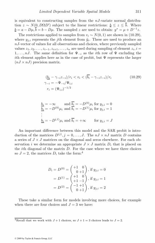
Limited Dependent Variable Spatial Models 311
is equivalent to constructing samples from the nJ-variate normal distribu-tion z ∼ N(0, DΩD′) subject to the linear restrictions: b ≤ z ≤ b. Whereb = a−Dμ, b = b−Dμ. The sampled z are used to obtain: y∗ = μ+D−1z.
The restrictions applied to samples from vi ∼ N(0, 1) are shown in (10.29),where yj,i represents the jth element from yi. These are used to produce annJ-vector of values for all observations and choices, where previously sampledvalues z1, z2, . . . , zi−1, zi+1, . . . , zn are used during sampling of element zi, i =1, . . . , nJ . The same definition for Ψ−i as the ith row of Ψ excluding theith element applies here as in the case of probit, but Ψ represents the larger(nJ × nJ) precision matrix.
(bi − γ−iz−i)/ri < vi < (bi − γ−iz−i)/ri (10.29)γ−i = −Ψ−i/Ψi,i
ri = (Ψi,i)−1/2
bi = −∞ and bi = −D(0)μi for yj,i = 0bi = −D(0)μi and bi = −D(1)μi for yj,i = 1...bi = −D(J)μi and bi = +∞ for yj,i = J
An important difference between this model and the SAR probit is intro-duction of the matrices D(j), j = 0, . . . , J . The nJ × nJ matrix D containsa series of J × J matrices on the diagonal and zeros elsewhere. For each ob-servation i we determine an appropriate J × J matrix Di that is placed onthe ith diagonal of the matrix D. For the case where we have three choicesso J = 2, the matrices Di take the form:4
Di = D(0) =(
+1 00 +1
), if yj,i = 0
= D(1) =(
+1 0+1 −1
), if yj,i = 1
= D(2) =(−1 +1
0 +1
), if yj,i = 2
These take a similar form for models involving more choices, for examplewhen there are four choices and J = 3 we have:
4Recall that we work with J + 1 choices, so J + 1 = 3 choices leads to J = 2.
© 2009 by Taylor & Francis Group, LLC
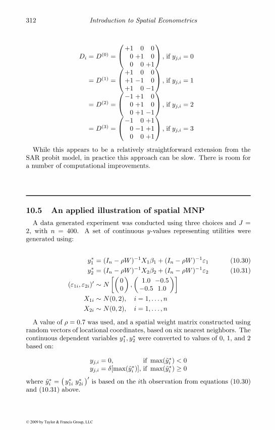
312 Introduction to Spatial Econometrics
Di = D(0) =
⎛⎝+1 0 00 +1 00 0 +1
⎞⎠ , if yj,i = 0
= D(1) =
⎛⎝+1 0 0+1 −1 0+1 0 −1
⎞⎠ , if yj,i = 1
= D(2) =
⎛⎝−1 +1 00 +1 00 +1 −1
⎞⎠ , if yj,i = 2
= D(3) =
⎛⎝−1 0 +10 −1 +10 0 +1
⎞⎠ , if yj,i = 3
While this appears to be a relatively straightforward extension from theSAR probit model, in practice this approach can be slow. There is room fora number of computational improvements.
10.5 An applied illustration of spatial MNP
A data generated experiment was conducted using three choices and J =2, with n = 400. A set of continuous y-values representing utilities weregenerated using:
y∗1 = (In − ρW )−1X1β1 + (In − ρW )−1ε1 (10.30)y∗2 = (In − ρW )−1X2β2 + (In − ρW )−1ε2 (10.31)
(ε1i, ε2i)′ ∼ N
[(00
),
(1.0 −0.5−0.5 1.0
)]X1i ∼ N(0, 2), i = 1, . . . , nX2i ∼ N(0, 2), i = 1, . . . , n
A value of ρ = 0.7 was used, and a spatial weight matrix constructed usingrandom vectors of locational coordinates, based on six nearest neighbors. Thecontinuous dependent variables y∗1 , y
∗2 were converted to values of 0, 1, and 2
based on:
yj,i = 0, if max(y∗i ) < 0yj,i = δ[max(y∗i )], if max(y∗i ) ≥ 0
where y∗i =(y∗1i y
∗2i
)′ is based on the ith observation from equations (10.30)and (10.31) above.
© 2009 by Taylor & Francis Group, LLC
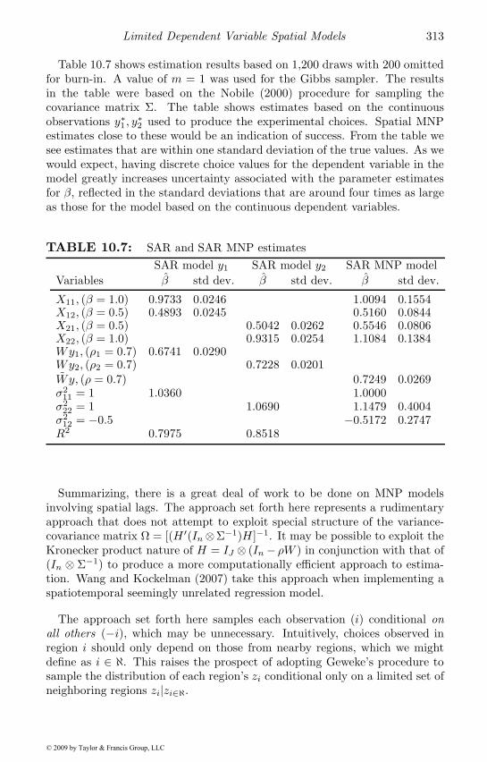
Limited Dependent Variable Spatial Models 313
Table 10.7 shows estimation results based on 1,200 draws with 200 omittedfor burn-in. A value of m = 1 was used for the Gibbs sampler. The resultsin the table were based on the Nobile (2000) procedure for sampling thecovariance matrix Σ. The table shows estimates based on the continuousobservations y∗1 , y∗2 used to produce the experimental choices. Spatial MNPestimates close to these would be an indication of success. From the table wesee estimates that are within one standard deviation of the true values. As wewould expect, having discrete choice values for the dependent variable in themodel greatly increases uncertainty associated with the parameter estimatesfor β, reflected in the standard deviations that are around four times as largeas those for the model based on the continuous dependent variables.
TABLE 10.7: SAR and SAR MNP estimatesSAR model y1 SAR model y2 SAR MNP model
Variables β std dev. β std dev. β std dev.
X11, (β = 1.0) 0.9733 0.0246 1.0094 0.1554X12, (β = 0.5) 0.4893 0.0245 0.5160 0.0844X21, (β = 0.5) 0.5042 0.0262 0.5546 0.0806X22, (β = 1.0) 0.9315 0.0254 1.1084 0.1384Wy1, (ρ1 = 0.7) 0.6741 0.0290Wy2, (ρ2 = 0.7) 0.7228 0.0201Wy, (ρ = 0.7) 0.7249 0.0269σ2
11 = 1 1.0360 1.0000σ2
22 = 1 1.0690 1.1479 0.4004σ2
12 = −0.5 −0.5172 0.2747R2 0.7975 0.8518
Summarizing, there is a great deal of work to be done on MNP modelsinvolving spatial lags. The approach set forth here represents a rudimentaryapproach that does not attempt to exploit special structure of the variance-covariance matrix Ω = [(H ′(In⊗Σ−1)H ]−1. It may be possible to exploit theKronecker product nature of H = IJ ⊗ (In− ρW ) in conjunction with that of(In ⊗ Σ−1) to produce a more computationally efficient approach to estima-tion. Wang and Kockelman (2007) take this approach when implementing aspatiotemporal seemingly unrelated regression model.
The approach set forth here samples each observation (i) conditional onall others (−i), which may be unnecessary. Intuitively, choices observed inregion i should only depend on those from nearby regions, which we mightdefine as i ∈ ℵ. This raises the prospect of adopting Geweke’s procedure tosample the distribution of each region’s zi conditional only on a limited set ofneighboring regions zi|zi∈ℵ.
© 2009 by Taylor & Francis Group, LLC
314 Introduction to Spatial Econometrics
The matrix H could be generalized to allow for different spatial depen-dence parameters associated with each choice. This variant of the model isimplemented in Autant-Bernard, LeSage and Parent (2008), where:
H =
⎛⎜⎝ In − ρ1W. . .
In − ρJW
⎞⎟⎠ (10.32)
Another avenue for exploration is the relative importance of spatial depen-dence versus dependence across choices. It may be that cross-choice covari-ance is unimportant relative to spatial dependence, allowing the model to besimplified by restricting Σ = IJ . The MNP model is often criticized as over-parameterized, so prior information such as this that reduces the number ofparameters to be estimated would be helpful.
10.5.1 Effects estimates for the spatial MNP model
Effects estimates for non-spatial MNP models estimated using maximumlikelihood methods are typically calculated by post-estimation simulation ofthe model with all but a single explanatory variable fixed. The impact ofchanging the single explanatory variable on the choice probabilities is used toassess the marginal impact of changes in the explanatory variables of interest.
Our Bayesian MCMC estimation procedure produces a set of continuouslatent dependent variable values that represent a proxy for unobserved utilityassociated with the J choices. The posterior mean of these latent variablevalues can of course be used to produce J posterior choice probabilities, withthe excluded J + 1 choice also recovered.
Most of the same insights regarding interpretation of marginal effects forthe SAR probit model apply to the SAR MNP model as well. For example,we can extend our example of burglaries on the decision to purchase a securitysystem to include purchasing a dog, or installing security lights. The SARMNP model implies that a change in burglaries (an explanatory variable inthe model) of neighboring homes j would have an effect on the probabilitythat homeowner i purchases a security system, a dog, or security lighting.The effect would depend on spatial proximity of homeowner i to j, capturedby the spatial weight matrix W as well as the strength of spatial dependencemeasured by the parameter ρ. A burglary at home j would have both a directeffect on the probability that homeowner j purchases a security system, adog or security lighting, as well as an indirect or spatial spillover effect onneighbors’ choices regarding these three alternatives. The total effect is thesum of these two effects for each choice alternative.
There are also some important qualifications that may apply to interpre-tation based on the particular model specification. For example, use of theblock diagonal dependence structure: InJ − ρW , or that shown in (10.32),
© 2009 by Taylor & Francis Group, LLC
Limited Dependent Variable Spatial Models 315
restricts us to a situation where the utility of choice j by an individual lo-cated in region i is not directly influenced by the utility of choice k �= j byan individual located in a neighboring region h �= i. Cross-choice influenceworks through dependence captured by the covariance structure Σ, ratherthan through spatial lags that embody cross-choice spatial dependence. Thissimplifies calculation of the marginal effects estimates, since changes in xkh,rwill not impact yji, when k �= j, and when h �= i.
The model could of course be extended along these lines by directly intro-ducing spatial lags for utility associated with the J choices being modeled ineach equation of the model. For example in the case of three choices whereJ = 2, we might use:
y1 = ρ11Wy1 + ρ12Wy2 +X1β1 + ε1
y2 = ρ21Wy1 + ρ22Wy2 +X2β2 + ε2
In this model, y1 and y2 represent n × 1 vectors containing indicators forobserved choices 1 and 2 across the n regions. The n× k matrices X1, X2 arealso arranged according to regions.
This type of model might be appropriate in situations where we are mod-eling the utility of a local government choosing to impose a payroll incometax (y1) versus a sales tax (y2). The utility of imposing a payroll tax mightdepend directly on whether neighboring governments have chosen to imple-ment a payroll tax (ρ11Wy1) or sales tax (ρ12Wy2). Similarly, the utilityassociated with the sales tax might depend on the existence of both payrolltaxes in neighboring governments, (ρ21Wy1) as well as sales taxes by neigh-bors (ρ22Wy2). Intuitively, this might arise because firms could relocate toavoid the payroll taxes, and local residents could alter shopping behavior toavoid sales taxes. Imposing the restriction that Σ = IJ for this model seemsreasonable, since cross-choice dependence is modeled in the mean part of themodel.
Calculating marginal effects for this type of model would require alteringour basic expression used to produce the scalar summary measures. If wedefine:
H =(In − ρ11W −ρ12W−ρ21W In − ρ22W
)X =
(X1 0k0k X2
)y =
(y1y2
)then, assuming Σ = IJ , we have a variance-covariance matrix: Ω = (H ′H)−1,with the associated precision matrix that would be subjected to the m-stepGibbs sampling procedure.
© 2009 by Taylor & Francis Group, LLC
316 Introduction to Spatial Econometrics
For this two-equation example, the SAR MNP effects are such that changesin an explanatory variable associated with say, equation j = 2 will impactobservations y1i, i = 1, . . . , n as well as y2i, i = 1, . . . , n. That is, ∂y1/∂x2r �=0 and ∂y2/∂x1r �= 0. This of course follows from allowing for cross-choiceimpacts in the mean component of the model, reflected by the spatial lagstructure, and the resulting: μ = H−1Xβ.
For the payroll versus sales tax example, we could use the model to ana-lyze the impact of changes in an explanatory variable such as levels of payrollincome in each location on the long-run steady state probabilities that lo-cal governments would rely on payroll versus sales taxes. The impact of anincrease in payroll income of one local government jurisdiction on the prob-ability of the own- and other-local governments adopting a payroll incometax versus sales tax, plus spatial spillover (indirect) effects on the probabilitythat neighboring governments adopt both payroll and sales taxes could beanalyzed using the scalar summary measures.
10.6 Spatially structured effects probit models
An alternative to SAR models for situations involving limited dependentvariables is a model that introduces a spatially structured random effectsvector (Smith and LeSage, 2004). This type of model was already introducedin the context of interregional trade flows in Chapter 8.
This hierarchical Bayesian model is shown in (10.33), where Uik, indexesutility in regions i = 1, . . . ,m for individuals k = 1, . . . , ni within each region.There are N =
∑mi=1 ni observations in the model, and we use wij to denote
the i, jth elements of the m×m spatial weight matrix W .
Uik = Xikβ + ξik (10.33)ξik = θi + εik
θi = ρ
m∑j=1
wijθj + ui
This model treats the unobserved component ξik as consisting of a region-specific effect θi as well as an individual effect εik. The regional effect param-eter θi captures unobserved common features for observations located withinregion i. The regional effects parameters are modeled using a SAR process:θi = ρ
∑mj=1 wijθj + ui which imposes a restriction that individuals located
within region i are likely to be similar to those from neighboring regions.The individualistic effects parameters are then assumed to be conditionallyindependent given the regional effects θi.
© 2009 by Taylor & Francis Group, LLC
Limited Dependent Variable Spatial Models 317
This model is a variation on a fixed effects model. Using matrix notationwe can express the model as in (10.34), where the m × 1 vector θ representsthe spatially structured effects.
y = Xβ + Δθ + ε (10.34)θ = ρWθ + u
u ∼ N(0, σ2uIm)
ε|θ ∼ N(0, V )
V =
⎛⎜⎝ v1In1
. . .vmInm
⎞⎟⎠ (10.35)
Δ =
⎛⎜⎝11
. . .1m
⎞⎟⎠ (10.36)
We accommodate heterogeneity across regions using a set of variance scalarsvi, i = 1, . . . ,m, and use 1i, i = 1, . . . ,m to denote an (ni × 1) vector of ones.The effects parameters need not be applied to all regions, for example whenworking with counties we might estimate state-level effects parameters. TheN ×m matrix Δ works to assign the same effect parameter to each of the nicounties in state i. Specifically, Δ contains row-elements i = 1, . . . ,m thatequal 1 if region (county) i is located in state m and zero otherwise. Thismodel interprets the parameters in the m × 1 vector θ as latent indicatorsfor unobservable/unmeasured state-level influences. These are restricted tofollow a SAR process, so neighboring states will exhibit similar effects levels.
The model also accommodates heterogeneity across the m broader regions(e.g. states) allowing for different variance scalars vi to be associated witheach of these regions. This is accomplished using the independent identicallydistributed chi-squared prior discussed in Chapter 5. All observations in eachstate (broader region) are assigned the same variance scalar parameter.
The spatial autoregressive structure placed on the effects parameters reflectsan implied prior for the vector θ conditional on ρ, σ2
u, V shown in (10.37).
π(θ|ρ, σ2u) ∝ (σ2
u)−m/2|B|exp
(− 1
2σ2u
θ′B′Bθ)
(10.37)
B = Im − ρW
Estimation of the spatially structured effects vector θ requires introductionof two additional parameters (ρ, σ2
u) to the model. One of these controls thestrength of spatial dependence between regions and the other controls thevariance/uncertainty of the prior spatial structure. Given these two scalar
© 2009 by Taylor & Francis Group, LLC
318 Introduction to Spatial Econometrics
parameters along with the spatial structure, the m effects parameters arecompletely determined. One could view the spatial connectivity matrix W asintroducing additional exogenous information that augments the sample datainformation. In contrast, the conventional fixed effects approach introducesmadditional parameters to be estimated without augmenting the sample datainformation.
There is also an implied prior density for ε conditional on θ, V which takesthe form:
π(ε|V ) ∝ |V |−1/2exp(−1
2ε′V −1ε
)(10.38)
Smith and LeSage (2004) provide details regarding Bayesian MCMC esti-mation of this hierarchical linear model, and the model is discussed in detailby Rossi, Allenby and McCulloch (2006). The binary dependent variables aretreated as choice outcomes that reflect latent underlying utilities followingAlbert and Chib (1993). The conditional posterior of zik for individual k inregion i takes the form of a normal distribution truncated at zero:
p(zik|z−ik, ρ, β, θ, σ2u, V, y) ∼
{N(x′iβ + θi, vi) left-truncated, if yi = 1N(x′iβ + θi, vi) right-truncated, if yi = 0
This model is considerably faster to estimate than the SAR probit modelbecause it relies on a smaller m ×m spatial component. Smith and LeSage(2004) decompose the m×m multivariate normal distribution for the effectsvector θ into a sequence of univariate normal distributions which are sam-pled to produce the effects parameter estimates. This is of course similar tothe approach of Geweke (1991) outlined here, but does not involve samplingfrom a truncated normal distribution, just a sequence of univariate normalsconditional on other elements of θ−i.
Interpreting the parameters β for this model is similar to that from anordinary probit model, so there are no spatial spillover effects in this model.However, we can use the spatially structured effects estimates for each regionto draw inferences regarding spatial variation in the model relationship. Theeffects parameters θ are centered on zero, so regions with negative and positiveand significant effects point to latent factors at work that are not included inthe explanatory variables matrix X .
An interesting extension of this model can be found in Wang and Kock-elman (2008a,b), who extend this model to allow for a set of
∑Mi=1 ni = N ,
individuals located in M regions across time periods t = 1, . . . , T . Theirmodel is dynamic, taking the form:
y∗ikt = λy∗ikt−1 +Xiktβ + θit + εikt (10.39)
where t indexes time periods, k individuals and i regions. This model allowsfor temporal dependence governed by the parameter λ. Each individual makes
© 2009 by Taylor & Francis Group, LLC

Limited Dependent Variable Spatial Models 319
a decision that is observed T times, so we have a balanced panel containingNT observations. The parameters θit and εikt are assumed iid distributedover time conditional on controlling for the influence of the lagged dependentvariable y∗ikt−1. The argument is that after controlling for time dependencein decisions, θit = θi and εikt = εik, for all t = 1, . . . , T .
The motivating example for this type of model given by Wang and Kock-elman (2008b) is an application to land development decisions. They arguethat land usage patterns depend strongly on pre-existing as well as existingconditions, and owner/developer expectations of future conditions (such aslocal and regional congestion, population, and school access). Future expec-tations are approximated using contemporaneous measures of access and landuse intensity, but Wang and Kockelman (2008b) argue that spatial correlationin unobserved factors is likely to remain.
They argue that land use conversion decisions can be viewed as an orderedprobit situation if we consider varying intensity levels of land development.As already noted, ordered probit models describe situations where there aremore than two choice outcomes, but the alternatives exhibit a natural orlogical ordering. As noted, in the simple cross-sectional case where individuali’s choices are independent from those of other individuals in the non-spatialmodel, the cut-point values φ can be determined by examining the maximum(and minimum) values of the latent data y∗i over all individuals i = 1, . . . , nwho have chosen alternative j.
φj−1 = max{max{y∗i : yi = j}, φj−1}φj+1 = min{min{y∗i : yi = j + 1}, φj+1}
Wang and Kockelman (2008a) point out that in a spatial model settingwhere choices of individuals are not independent, but exhibit both space aswell as time dependence, this line of argument no longer holds. To pursuethis, we consider the (multivariate) normal prior placed on the cut-point pa-rameters by Wang and Kockelman (2008a).
φ ∼ N(g,Q)δ(φ1 < φ2 < . . . , φJ−1) (10.40)
where g is a vector of prior means (with elements gj) and Q is a (diagonal)matrix containing prior variances, which we label qj . Recall, δ(A) is an in-dicator function for each event A, so δ(A) = 1 for outcomes where A occursand δ(A) = 0 otherwise. This acts as a constraint to ensure probabilitiesderived from the thresholds are positive. Of course, in the limit with all ele-ments of gj = 0 and the variances qj infinite, we have the flat prior used inour discussion of the ordered probit model in Section 10.2. The conditionalposterior for these parameters takes the form in (10.41), where we use � todenote conditioning arguments other than φ−j consisting of other parametersin the model.
© 2009 by Taylor & Francis Group, LLC
320 Introduction to Spatial Econometrics
p(φj |φ−j , �) ∝ δ(φj−1 < φj < φj+1)exp(− 1
2qj(φj − gj)2
)(10.41)
Of course, in the limiting case of a flat prior where qj → ∞, this collapses toour Uniform distribution:
p(φj |φ−j , �) ∝ U(φj−1 < φj < φj+1), j = 2, . . . , J − 1 (10.42)
The bounding values are determined by examining the maximum (and min-imum) values of the latent data y∗ikt over all individuals k = 1, . . . , ni, and allregions i = 1, . . . ,M who have chosen alternative j at all times t = 1, . . . , T .In this general spatial model, individuals’ choices are spatially dependent onthose of individuals in nearby regions and past time periods leading to:
φj−1 = max{max{y∗ikt : yikt = j}, φj−1}φj+1 = min{min{y∗ikt : yikt = j + 1}, φj+1}
Because of the dependence of y∗ikt on other time periods and regions, thelower and upper bounds in this model also exhibit dependence. This can leadto a multimodal posterior distribution for these parameters.
10.7 Chapter summary
We have seen that Bayesian treatment of observable binary and polychoto-mous dependent variables y as indicators of latent underlying utilities y∗ canbe useful in modeling limited dependent variables that exhibit spatial depen-dence. Albert and Chib (1993) argue that if the vector of latent utilities y∗
were known, p(β, ρ, |y∗) = p(β, ρ|y∗, y), allowing us to view y∗ as an addi-tional set of parameters to be estimated. This leads to a (joint) conditionalposterior distribution for our model parameters (conditioning on both y∗, y)that takes the same form as the Bayesian estimation problem from Chapter 5.
For models involving spatial dependence, we need to perform some com-putational work to sample from the conditional posterior distribution for theparameters y∗ that we introduce in the model. The spatial dependence struc-ture leads to a multivariate truncated normal distribution for these param-eters, rather than the simple univariate truncated normal distribution thatarises in the case of independent sample data. However, we showed thata procedure proposed by Geweke (1991) can be used to successfully samplefrom this conditional distribution. The procedure samples from this multi-variate truncated normal distribution by breaking the task into an m-step
© 2009 by Taylor & Francis Group, LLC
Limited Dependent Variable Spatial Models 321
Gibbs sampler that carries out m-draws from a series of n univariate con-ditional distributions. These m-draws provide an asymptotically consistentestimate for the parameters y∗. These are then used when sampling from theconditional distributions of the remaining model parameters, β, ρ.
Despite the drawback arising from the computational intensity of this ap-proach, there are a number of desirable aspects as well. One point is thatimplementation of the method is quite simple from a coding standpoint. Wesimply need to add code to our existing routine for MCMC estimation of theBayesian SAR model to implement the m-step Gibbs sampler, with the re-maining code unchanged. This amounts to a few lines of code that calls aspecialized function to carry out the truncated multivariate normal samplingtask.
© 2009 by Taylor & Francis Group, LLC