arX

iv:g

r-qc

/040

9061

v3 9

Feb

200

5

Proceedings of the II International Conference on Fundamental InteractionsPedra Azul, Brazil, June 2004

INTRODUCTION TO LOOP QUANTUM GRAVITY AND SPIN

FOAMS

ALEJANDRO PEREZ∗

Institute for Gravitational Physics and Geometry, Penn State University, 104 Davey Lab

University Park, PA 16802, USA

and

Centre de Physique Theorique CNRS

Luminy Case 907 F-13288 Marseille cedex 9, France†

These notes are a didactic overview of the non perturbative and background independentapproach to a quantum theory of gravity known as loop quantum gravity. The definitionof real connection variables for general relativity, used as a starting point in the program,is described in a simple manner. The main ideas leading to the definition of the quantumtheory are naturally introduced and the basic mathematics involved is described. Themain predictions of the theory such as the discovery of Planck scale discreteness ofgeometry and the computation of black hole entropy are reviewed. The quantizationand solution of the constraints is explained by drawing analogies with simpler systems.Difficulties associated with the quantization of the scalar constraint are discussed.

In a second part of the notes, the basic ideas behind the spin foam approach arepresented in detail for the simple solvable case of 2+1 gravity. Some results and ideasfor four dimensional spin foams are reviewed.

Keywords: Quantum Gravity; Loop variables; Non-perturbative methods; Path Integrals;Yang-Mills theory.

1. Introduction: why non perturbative quantum gravity?

The remarkable experimental success of the standard model in the description of

fundamental interactions is the greatest achievement of (relativistic) quantum field

theory. Standard quantum field theory provides an accomplished unification be-

tween the principles of quantum mechanics and special relativity. The standard

model is a very useful example of a quantum field theory on the fixed background

geometry of Minkowski spacetime. As such, the standard model can only be re-

garded as an approximation of the description of fundamental interactions valid

when the gravitational field is negligible. The standard model is indeed a very good

approximation describing particle physics in the lab and in a variety of astrophysical

situations because of the weakness of the gravitational force at the scales of interest

(see for instance the lecture by Rogerio Rosenfeld1). Using the techniques of quan-

tum field theory on curved spacetimes2 one might hope to extend the applicability

∗Penn State University, 104 Davey Lab, University Park, PA 16802, USA.†State completely without abbreviations, the affiliation and mailing address, including country.

1

2 Alejandro Perez

of the standard model to situations where a non trivial, but weak, gravitational

field is present. These situations are thought to be those where the spacetime cur-

vature is small in comparison with the Planck scale, although a clear justification

for its regime of validity in strong gravitational fields seems only possible when a

full theory of quantum gravity is available. Having said this, there is a number of

important physical situations where we do not have any tools to answer even the

simplest questions. In particular classical general relativity predicts the existence of

singularities in physically realistic situations such as those dealing with black hole

physics and cosmology. Near spacetime singularities the classical description of the

gravitational degrees of freedom simply breaks down. Questions related to the fate

of singularities in black holes or in cosmological situations as well as those related

with apparent information paradoxes are some of the reasons why we need a theory

of quantum gravity. This new theoretical framework—yet to be put forward—aims

at a consistent description unifying or, perhaps more appropriately, underlying the

principles of general relativity and quantum mechanics.

The gravitational interaction is fundamentally different from all the other known

forces. The main lesson of general relativity is that the degrees of freedom of the

gravitational field are encoded in the geometry of spacetime. The spacetime geom-

etry is fully dynamical: in gravitational physics the notion of absolute space on top

of which ‘things happen’ ceases to make sense. The gravitational field defines the

geometry on top of which its own degrees of freedom and those of matter fields

propagate. This is clear from the perspective of the initial value formulation of gen-

eral relativity, where, given suitable initial conditions on a 3-dimensional manifold,

Einstein’s equations determine the dynamics that ultimately allows for the recon-

struction of the spacetime geometry with all the matter fields propagating on it. A

spacetime notion can only be recovered a posteriori once the complete dynamics of

the coupled geometry-matter system is worked out. Matter affects the dynamics of

the gravitational field and is affected by it through the non trivial geometry that

the latter defines a. General relativity is not a theory of fields moving on a curved

background geometry; general relativity is a theory of fields moving on top of each

other4.

In classical physics general relativity is not just a successful description of the

nature of the gravitational interaction. As a result of implementing the principles

of general covariance, general relativity provides the basic framework to assessing

the physical world by cutting all ties to concepts of absolute space. It represents

the result of the long-line of developments that go all the way back to the thought

experiments of Galileo about the relativity of the motion, to the arguments of

Mach about the nature of space and time, and finally to the magnificent conceptual

synthesis of Einstein’s: the world is relational. There is no well defined notion of

absolute space and it only makes sense to describe physical entities in relation to

aSee for instance Theorem 10.2.2 in 3.

INTRODUCTION TO LOOP QUANTUM GRAVITY AND SPIN FOAMS 3

other physical entities. This conceptual viewpoint is fully represented by the way

matter and geometry play together in general relativity. The full consequences of

this in quantum physics are yet to be unveiledb.

When we analyze a physical situation in pre-general-relativistic physics we sep-

arate what we call the system from the relations to other objects that we call the

reference frame. The spacetime geometry that we describe with the aid of coordi-

nates and a metric is a mathematical idealization of what in practice we measure

using rods and clocks. Any meaningful statement about the physics of the system

is a statement about the relation of some degrees of freedom in the system with

those of what we call the frame. The key point is that when the gravitational field is

trivial there exist a preferred set of physical systems whose dynamics is very simple.

These systems are inertial observers; for instance one can think of them as given by

a spacial grid of clocks synchronized by the exchange of light signals. These physical

objects provide the definition of inertial coordinates and their mutual relations can

be described by a Minkowski metric. As a result in pre-general relativistic physics

we tend to forget about rods and clocks that define (inertial) frames and we talk

about time t and position x and distances measure using the flat metric ηabc. How-

ever, what we are really doing is comparing the degrees of freedom of our system

with those of a space grid of world-lines of physical systems called inertial observers.

From this perspective, statements in special relativity are in fact diffeomorphism in-

variant. The physics from the point of view of an experimentalist—dealing with the

system itself, clocks, rods, and their mutual relations—is completely independent of

coordinates. In general relativity this property of the world is confronted head on:

only relational (coordinate-independent, or diffeomorphism invariant) statements

are meaningful (see discussion about the hole argument in 4). There are no sim-

ple family of observers to define physical coordinates as in the flat case, so we use

arbitrary labels (coordinates) and require the physics to be independent of them.

In this sense, the principles of general relativity state some basic truth about the

nature of the classical world. The far reaching consequences of this in the quantum

realm are certainly not yet well understood.d However, it is very difficult to imagine

that a notion of absolute space would be saved in the next step of development

of our understanding of fundamental physics. Trying to build a theory of quantum

gravity based on a notion of background geometry would be, from this perspective,

reminiscent of the efforts by contemporaries of Copernicus of describing planetary

motion in terms of the geocentric framework.

bFor a fascinating account of the conceptual subtleties of general relativity see Rovelli’s book4.cIn principle we first use rods and clocks to realize that in the situation of interests (e.g. anexperiment at CERN) the gravitational field is trivial and then we just encode this information ina fix background geometry: Minkowski spacetime.dA reformulation of quantum mechanics from a relational perspective has been introducedby Rovelli5 and further investigated in the context of conceptual puzzles of quantummechanics6,7,8,9,10. It is also possible that a radical change in the paradigms of quantum me-chanics is necessary in the conceptual unification of gravity and the quantum11,12,13,14.

4 Alejandro Perez

1.1. Perturbative quantum gravity

Let us make some observations about the problems of standard perturbative quan-

tum gravity. In doing so we will revisit the general discussion above, in a special

situation. In standard perturbative approaches to quantum gravity one attempts to

describe the gravitational interaction using the same techniques applied to the defi-

nition of the standard model. As these techniques require a notion of non dynamical

background one (arbitrarily) separates the degrees of freedom of the gravitational

field in terms of a background geometry ηab for a, b = 1 · · · 4—fixed once and for

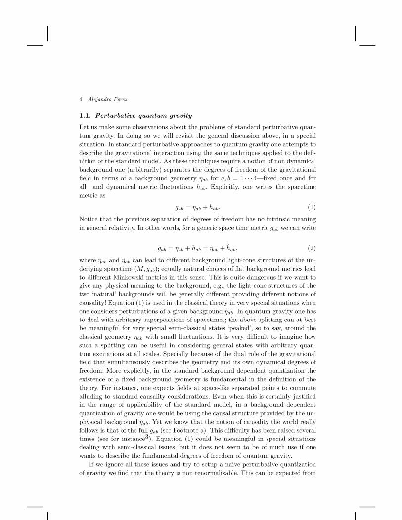
all—and dynamical metric fluctuations hab. Explicitly, one writes the spacetime

metric as

gab = ηab + hab. (1)

Notice that the previous separation of degrees of freedom has no intrinsic meaning

in general relativity. In other words, for a generic space time metric gab we can write

gab = ηab + hab = ηab + hab, (2)

where ηab and ηab can lead to different background light-cone structures of the un-

derlying spacetime (M, gab); equally natural choices of flat background metrics lead

to different Minkowski metrics in this sense. This is quite dangerous if we want to

give any physical meaning to the background, e.g., the light cone structures of the

two ‘natural’ backgrounds will be generally different providing different notions of

causality! Equation (1) is used in the classical theory in very special situations when

one considers perturbations of a given background ηab. In quantum gravity one has

to deal with arbitrary superpositions of spacetimes; the above splitting can at best

be meaningful for very special semi-classical states ‘peaked’, so to say, around the

classical geometry ηab with small fluctuations. It is very difficult to imagine how

such a splitting can be useful in considering general states with arbitrary quan-

tum excitations at all scales. Specially because of the dual role of the gravitational

field that simultaneously describes the geometry and its own dynamical degrees of

freedom. More explicitly, in the standard background dependent quantization the

existence of a fixed background geometry is fundamental in the definition of the

theory. For instance, one expects fields at space-like separated points to commute

alluding to standard causality considerations. Even when this is certainly justified

in the range of applicability of the standard model, in a background dependent

quantization of gravity one would be using the causal structure provided by the un-

physical background ηab. Yet we know that the notion of causality the world really

follows is that of the full gab (see Footnote a). This difficulty has been raised several

times (see for instance3). Equation (1) could be meaningful in special situations

dealing with semi-classical issues, but it does not seem to be of much use if one

wants to describe the fundamental degrees of freedom of quantum gravity.

If we ignore all these issues and try to setup a naive perturbative quantization

of gravity we find that the theory is non renormalizable. This can be expected from

INTRODUCTION TO LOOP QUANTUM GRAVITY AND SPIN FOAMS 5

Fig. 1. The larger cone represents the light-cone at a point according to the ad hoc backgroundηab. The smaller cones are a cartoon representation of the fluctuations of the true gravitationalfield represented by gab.

dimensional analysis as the quantity playing the role of the coupling constant turns

out to be the Planck length ℓp. The non renormalizability of perturbative gravity

is often explained through an analogy with the (non-renormalizable) Fermi’s four

fermion effective description of the weak interaction15. Fermi’s four fermions theory

is known to be an effective description of the (renormalizable) Weinberg-Salam

theory. The non renormalizable UV behavior of Fermi’s four fermion interaction is

a consequence of neglecting the degrees of freedom of the exchanged massive gauge

bosons which are otherwise disguised as the dimension-full coupling ΛFermi ≈ 1/m2W

at momentum transfer much lower than the mass of the W particle (q2 << m2W ).

A similar view is applied to gravity to promote the search of a more fundamental

theory which is renormalizable or finite (in the perturbative sense) and reduces

to general relativity at low energies. From this perspective it is argued that the

quantization of general relativity is a hopeless attempt to quantizing a theory that

does not contain the fundamental degrees of freedom.

These arguments, based on background dependent concepts, seem at the very

least questionable in the case of gravity. Although one should expect the notion of a

background geometry to be useful in certain semi-classical situations, the assump-

tion that such structure exists all the way down to the Planck scale is inconsistent

with what we know about gravity and quantum mechanics. General considerations

indicate that standard notions of space and time are expected to fail near the Planck

scale ℓpe. From this viewpoint the non renormalizability of perturbative quantum

eFor instance a typical example is to use a photon to measure distance. The energy of the photonin our lab frame is given by Eγ = hc/λ. We put the photon in a cavity and produce a standingwave measuring the dimensions of the cavity in units of the wavelength. The best possible precisionis attained when the Schwarzschild radius corresponding to energy of the photon is of the orderof its wavelength. Beyond that the photon can collapse to form a black hole around some of themaxima of the standing wave. This happens for a value λc for which λc ≈ GEγ/c4 = hG/(λcc3).The solution is λc ≈

√hG/c3 which is Planck length.

6 Alejandro Perez

gravity is indicative of the inconsistency of the separation of degrees of freedom

in (1). The nature of spacetime is expected to be very different from the classical

notion in quantum gravity. The treatment that uses (1) as the starting point is

assuming a well defined notion of background geometry at all scales which directly

contradicts these considerations.

In fact one could read the issues of divergences in an alternative way. The ac-

cepted jargon is that in a renormalizable theory the microscopic physics does not

affect low energy processes as its effects can be recast in simple redefinition of a

finite set of parameters, i.e., renormalization. In the case of gravity this miracle does

not happen. All correlation functions blow up and one would need to add an infinite

number of corrections to the original Lagrangian when integrating out microscopic

physical degrees of freedom. Now imagine for the moment that a non perturba-

tive quantization of general relativity was available. If we now want to recover a

‘low energy effective’ description of a physical situation —where (low energy) phys-

ical considerations single out a preferred background—we would expect the need

of increasingly higher derivative correction terms to compensate the fact the ‘high

energy’f degrees of freedom know nothing about that low energy background. In

this sense the objections raised above to the violent and un-natural splitting (1) are

related to the issue of non renormalizability of general relativity. The nature of the

gravitational interaction is telling us that the standard paradigm of renormalization

(based on the notion of a fixed background) is no longer applicable. A reformulation

of quantum field theory is necessary to cope with background independence.

It is possible that new degrees of freedom would become important at more

fundamental scales. After all, that is the story of the path that lead to the standard

model where higher energy experiments has often lead to the discovery of new in-

teractions. It is also possible that including these degrees of freedom might be very

important for the consistency of the theory of quantum gravity. However, there is

constraint that seem hardly avoidable: if we want to get a quantum theory that

reproduces gravity in the semi-classical limit we should have a background inde-

pendent formalism. In loop quantum gravity one stresses this viewpoint. The hope

is that learning how to define quantum field theory in the absence of a background

is a key ingredient in a recipe for quantum gravity. Loop quantum gravity uses the

quantization of general relativity as a playground to achieve this goal.

I would like to finish this subsection with a quote of Weinberg’s 1980 paper that

would serve as introduction for the next section:

“It is possible that this problem—the non renormalizability of general relativity—

fThe notion of energy is observer dependent in special relativity. In the background independentcontext is not even defined. We use the terminology ‘high (low) energy’ in this introduction to referto the fundamental (semi-classical) degrees of freedom in quantum gravity. However, the readershould not take this too literally. In fact if one tries to identify the fundamental degrees of freedomof quantum gravity with a preferred observer conflict with observation seem inevitable16,17,18.

INTRODUCTION TO LOOP QUANTUM GRAVITY AND SPIN FOAMS 7

has arisen because the usual flat-space formalism of quantum field theory simply

cannot be applied to gravitation. After all, gravitation is a very special phenomenon,

involving as it does the very topology of space and time”

All these considerations make the case for a background independent approach

to quantum gravity. The challenge is to define quantum field theory in the absence

of any preestablished notion of distance: quantum field theory without a metric.

1.2. Loop quantum gravity

Loop quantum gravity is an attempt to define a quantization of gravity paying spe-

cial attention to the conceptual lessons of general relativity (the reader is encouraged

to read Rovelli’s book: Quantum Gravity4 as well as the recent review by Ashtekar

and Lewandowski19. For a detailed account of the mathematical techniques in-

volved in the construction of the theory see Thiemann’s book20). The theory is

explicitly formulated in a background independent, and therefore, non perturba-

tive fashion. The theory is based on the Hamiltonian (or canonical) quantization

of general relativity in terms of variables that are different from the standard met-

ric variables. In terms of these variables general relativity is cast into the form of a

background independent SU(2) gauge theory partly analogous to SU(2) Yang-Mills

theory. The main prediction of loop quantum gravity (LQG) is the discreteness21,22

of the spectrum of geometrical operators such as area and volume. The discreteness

becomes important at the Planck scale while the spectrum of geometric operators

crowds very rapidly at ‘low energy scales’ (large geometries). This property of the

spectrum of geometric operators is consistent with the smooth spacetime picture of

classical general relativity.

Thus it is not surprising that perturbative approaches would lead to inconsisten-

cies. In splitting the gravitational field degrees of freedom as in (1) one is assuming

the existence of a background geometry which is smooth all the way down to the

Planck scale. As we consider contributions from ‘higher energies’, this assumption

is increasingly inconsistent with the fundamental structure discovered in the non

perturbative treatment.

The theory is formulated in four dimensions. Matter can be coupled to the

gravitational degrees of freedom and the inclusion of matter has been studied in

great detail. However, throughout these lectures we will study the pure gravita-

tional sector in order simplify the presentation. On the super-symmetric extension

of canonical loop quantum gravity see 23,24,25,26,27. A spin foam model for 3d

super-gravity has been defined by Livine and Oeckl28.

Despite the achievements of LQG there remain important issues to be addressed.

There are difficulties of a rather technical nature related to the complete charac-

terization of dynamics and the quantization of the so-called scalar constraint. We

will review these once we have introduced the basic formalism. The most important

question, however, remains open: whether the semi-classical limit of the LQG is

8 Alejandro Perez

consistent with general relativity and the Standard Model.

Before starting with the more technical material let us say a few words regard-

ing unification. In loop quantum gravity matter is essentially added by coupling

general relativity with it at the classical level and then performing the (background

independent) canonical quantization. At this stage of development of the approach

it is not clear if there is some restriction in the kind of interactions allowed or if

degrees of freedom corresponding to matter could arise in some natural way directly

from those of geometry. However, there is a unification which is addressed head on

by LQG: the need to find a common framework in which to describe quantum field

theories in the absence of an underlying spacetime geometry. The implications of

this are far from being fully developed.

2. Hamiltonian formulation of general relativity: the new variables

In this section we introduce the variables that are used in the definition of loop

quantum gravity. We will present the SU(2) Ashtekar-Barbero variables by starting

with conventional ADM variables, introducing triads at the canonical level, and

finally performing the well known canonical transformation that leads to the new

variables. This is, in my opinion, the simplest way to get to the new variables.

For a derivation that emphasizes the covariant four dimensional character of these

variables see 19.

2.1. Canonical analysis in ADM variables

The action of general relativity in metric variables is given by the Einstein-Hilbert

action

I[gµν ] =1

2κ

∫dx4 √−gR, (3)

where κ = 8πG/c3 = 8πℓ2p/~, g is the determinant of the metric gab and R is the

Ricci scalar. The details of the Hamiltonian formulation of this action in terms

of ADM variables can be found in3. One introduces a foliation of spacetime in

terms of space-like three dimensional surfaces Σ. For simplicity we assume Σ has

no boundaries. The ten components of the spacetime metric are replaced by the six

components of the induced Riemannian metric qab of Σ plus the three components

of the shift vector Na and the lapse function N . In terms of these variables, after

performing the standard Legendre transformation, the action of general relativity

becomes

I[qab, πab, Na, N ] =

1

2κ

∫dt

∫

Σ

dx3 [πabqab

+2Nb∇(3)a(q−1/2πab) +N(q1/2[R(3) − q−1πcdπ

cd +1

2q−1π2])], (4)

where πab are the momenta canonically conjugate to the space metric qab, π =

πabqab, ∇(3)a is the covariant derivative compatible with the metric qab, q is the

INTRODUCTION TO LOOP QUANTUM GRAVITY AND SPIN FOAMS 9

determinant of the space metric and R(3) is the Ricci tensor of qab. The momenta

πab are related to the extrinsic curvature Kabg of Σ by

πab = q−1/2(Kab −Kqab) (5)

where K = Kabqab and indices are raised with qab. Variations with respect to the

lapse and shift produce the four constraint equations:

−V b(qab, πab) = 2∇(3)

a(q−1/2πab) = 0, (6)

and

−S(qab, πab) = (q1/2[R(3) − q−1πcdπ

cd + 1/2q−1π2]) = 0. (7)

V b(qab, πab) is the so-called vector constraint and S(qab, π

ab) is the scalar constraint.

With this notation the action can be written as

I[qab, πab, Na, N ] =

1

2κ

∫dt

∫

Σ

dx3[πabqab −NbV

b(qab, πab) −NS(qab, π

ab)],

(8)

where we identify the Hamiltonian density H(qab, πab, Na, N) = NbV

b(qab, πab) +

NS(qab, πab). The Hamiltonian is a linear combination of (first class) constraints,

i.e., it vanishes identically on solutions of the equations of motion. This is a generic

property of generally covariant systems. The symplectic structure can be read off

the previous equations, namelyπab(x), qcd(y)

= 2κ δa

(cδbd)δ(x, y),

πab(x), πcd(y)

= qab(x), qcd(y) = 0 (9)

There are six configuration variables qab and four constraint equations (6) and (7)

which implies the two physical degrees of freedom of gravity h.

2.2. Toward the new variables: the triad formulation

Now we do a very simple change of variables. The idea is to use a triad (a set of

three 1-forms defining a frame at each point in Σ) in terms of which the metric qab

becomes

qab = eiae

jbδij , (10)

where i, j = 1, 2, 3. Using these variables we introduce the densitized triad

Eai :=

1

2ǫabcǫijke

jbe

kc . (11)

Using this definition, the inverse metric qab can be related to the densitized triad

as follows

qqab = Eai E

bjδ

ij . (12)

gThe extrinsic curvature is given by Kab = 12Lnqab where na is the unit normal to Σ.

hThis counting of physical degrees of freedom is correct because the constraints are first class29.

10 Alejandro Perez

We also define

Kia :=

1√det(E)

KabEbjδ

ij . (13)

A simple exercise shows that one can write the canonical term in (8) as

πabqab = −πabqab = 2Ea

i Kia (14)

and that the constraints V a(qab, πab) and S(qab, π

ab) can respectively be written

as V a(Eai ,K

ia) and S(Ea

i ,Kia). Therefore we can rewrite (8) in terms of the new

variables. However, the new variables are certainly redundant, in fact we are using

the nine Eai to describe the six components of qab. The redundancy has a clear ge-

ometrical interpretation: the extra three degrees of freedom in the triad correspond

to our ability to choose different local frames eia by local SO(3) rotations acting in

the internal indices i = 1, 2, 3. There must then be an additional constraint in terms

of the new variables that makes this redundancy manifest. The missing constraint

comes from (13): we overlooked the fact that Kab = Kba or simply that K[ab] = 0.

By inverting the definitions (11) and (13) in order to write Kab in terms of Eai and

Kia one can show that the condition K[ab] = 0 reduces to

Gi(Eaj ,K

ja) := ǫijkE

ajKka = 0. (15)

Therefore we must include this additional constraint to (8) if we want to use the

new triad variables. With all this the action of general relativity becomes

I[Eaj ,K

ja, Na, N,N

j ] =

1

κ

∫dt

∫

Σ

dx3[Ea

i Kia −NbV

b(Eaj ,K

ja) −NS(Ea

j ,Kja) −N iGi(E

aj ,K

ja)

],(16)

where the explicit form of the constraints in terms of triad variables can be worked

out from the definitions above. The reader is encouraged to do this exercise but

it is not going to be essential to understanding what follows (expressions for the

constraints can be found in reference30). The symplectic structure now becomes

Ea

j (x),Kib(y)

= κ δa

b δijδ(x, y),

Ea

j (x), Ebi (y)

=

Kj

a(x),Kib(y)

= 0 (17)

The counting of physical degrees of freedom can be done as before.

2.3. New variables: the Ashtekar-Barbero connection variables

The densitized triad (11) transforms in the vector representation of SO(3) under

redefinition of the triad (10). Consequently, so does its conjugate momentum Kia

(see equation (13)). There is a natural so(3)-connection that defines the notion of

covariant derivative compatible with the triad. This connection is the so-called spin

connection Γia and is characterized as the solution of Cartan’s structure equations

∂[aeib] + ǫijkΓj

[aekb] = 0 (18)

INTRODUCTION TO LOOP QUANTUM GRAVITY AND SPIN FOAMS 11

The solution to the previous equation can be written explicitly in terms of the triad

components

Γia = −1

2ǫijke

bj

(∂[ae

kb] + δklδmse

cl e

ma ∂be

sc

), (19)

where eai is the inverse triad (ea

i eja = δj

i ). We can obtain an explicit function of the

densitized triad—Γia(Eb

j )—inverting (11) from where

eia =

1

2

ǫabcǫijkEb

jEck√

|det(E)|and ea

i =sgn(det(E)) Ea

i√|det(E)|

. (20)

The spin connection is an so(3) connection that transforms in the standard inho-

mogeneous way under local SO(3) transformations. The Ashtekar-Barbero31,32,33

variables are defined by the introduction of a new connection Aia given by

Aia = Γi

a + γKia, (21)

where γ is any non vanishing real number called the Immirzi parameter34. The

new variable is also an so(3) connection as adding a quantity that transforms as a

vector to a connection gives a new connection. The remarkable fact about this new

variable is that it is in fact conjugate to Eia. More precisely the Poisson brackets of

the new variables areEa

j (x), Aib(y)

= κ γδa

b δijδ(x, y),

Ea

j (x), Ebi (y)

=

Aj

a(x), Aib(y)

= 0. (22)

All the previous equations follow trivially from (17) except forAj

a(x), Aib(y)

= 0

which requires more calculations. The reader is invited to check it.

Using the connection variables the action becomes

I[Eaj , A

ja, Na, N,N

j ] =

1

κ

∫dt

∫

Σ

dx3[Ea

i Aai −N bVb(E

aj , A

ja) −NS(Ea

j , Aja) −N iGi(E

aj , A

ja)

], (23)

where the constraints are explicitly given by:

Vb(Eaj , A

ja) = Ea

j Fab − (1 + γ2)KiaGi (24)

S(Eaj , A

ja) =

Eai E

bj√

det(E)

(ǫijkF

kab − 2(1 + γ2)Ki

[aKjb]

)(25)

Gi(Eaj , A

ja) = DaE

ai , (26)

where Fab = ∂aAib − ∂bA

ia + ǫijkA

jaA

kb is the curvature of the connection Ai

a and

DaEai = ∂aE

ai + ǫ k

ij AjaE

ak is the covariant divergence of the densitized triad. We

have seven (first class) constraints for the 18 phase space variables (Aia, E

bj ). In ad-

dition to imposing conditions among the canonical variables, first class constraints

are generating functionals of (infinitesimal) gauge transformations. From the 18-

dimensional phase space of general relativity we end up with 11 fields necessary

12 Alejandro Perez

to coordinatize the constraint surface on which the above seven conditions hold.

On that 11-dimensional constraint surface, the above constraint generate a seven-

parameter-family of gauge transformations. The reduce phase space is four dimen-

sional and therefore the resulting number of physical degrees of freedom is two, as

expected.

The constraint (26) coincides with the standard Gauss law of Yang-Mills theory

(e.g. ~∇ · ~E = 0 in electromagnetism). In fact if we ignore (24) and (25) the phase

space variables (Aia, E

bj ) together with the Gauss law (26) characterize the physical

phase space of an SU(2)i Yang-Mills (YM) theory. The gauge field is given by

the connection Aia and its conjugate momentum is the electric field Eb

j . Yang-Mills

theory is a theory defined on a background spacetime geometry. Dynamics in such a

theory is described by a non vanishing Hamiltonian—the Hamiltonian density of YM

theory being H = EiaE

ai +Bi

aBai . General relativity is a generally covariant theory

and coordinate time plays no physical role. The Hamiltonian is a linear combination

of constraints.j Dynamics is encoded in the constraint equations (24),(25), and (26).

In this sense we can regard general relativity in the new variables as a background

independent relative of SU(2) Yang-Mills theory. We will see in the sequel that

the close similarity between these theories will allow for the implementation of

techniques that are very natural in the context of YM theory.

2.3.1. Gauge transformations

Now let us analyze the structure of the gauge transformations generated by the

constraints (24),(25), and (26). From the previous paragraph it should not be sur-

prising that the Gauss law (26) generates local SU(2) transformations as in the case

of YM theory. Explicitly, if we define the smeared version of (26) as

G(α) =

∫

Σ

dx3 αiGi(Aia, E

ai ) =

∫

Σ

dx3αiDaEai , (27)

a direct calculation implies

δGAia =

Ai

a, G(α)

= −Daαi and δGE

ai = Ea

i , G(α) = [E,α]i . (28)

iThe constraint structure does not distinguish SO(3) from SU(2) as both groups have the sameLie algebra. From now on we choose to work with the more fundamental (universal covering) groupSU(2). In fact this choice is physically motivated as SU(2) is the gauge group if we want to includefermionic matter35,36,37.jIn the physics of the standard model we are used to identifying the coordinate t with the physicaltime of a suitable family of observers. In the general covariant context of gravitational physicsthe coordinate time t plays the role of a label with no physical relevance. One can arbitrarilychange the way we coordinatize spacetime without affecting the physics. This redundancy in thedescription of the physics (gauge symmetry) induces the appearance of constraints in the canonicalformulation. The constraints in turn are the generating functions of these gauge symmetries. TheHamiltonian generates evolution in coordinate time t but because redefinition of t is pure gauge,the Hamiltonian is a constraint itself, i.e. H = 0 on shell38,29. More on this in the next section.

INTRODUCTION TO LOOP QUANTUM GRAVITY AND SPIN FOAMS 13

If we write Aa = Aiaτi ∈ su(2) and Ea = Ea

i τi ∈ su(2), where τi are generators of

SU(2), we can write the finite version of the previous transformation

A′a = gAag

−1 + g∂ag−1 and Ea′ = gEag−1, (29)

which is the standard way the connection and the electric field transform under

gauge transformations in YM theory.

The vector constraint (24) generates three dimensional diffeomorphisms of Σ.

This is clear from the action of the smeared constraint

V (Na) =

∫

Σ

dx3 NaVa(Aia, E

ai ) (30)

on the canonical variables

δVAia =

Ai

a, V (Na)

= LNAia and δVE

ai = Ea

i , V (Na) = LNEai , (31)

where LN denotes the Lie derivative in the Na direction. The exponentiation of

these infinitesimal transformations leads to the action of finite diffeomorphisms on

Σ.

Finally, the scalar constraint (25) generates coordinate time evolution (up to

space diffeomorphisms and local SU(2) transformations). The total Hamiltonian

H [α,Na, N ] of general relativity can be written as

H(α,Na, N) = G(α) + V (Na) + S(N), (32)

where

S(N) =

∫

Σ

dx3 NS(Aia, E

ai ). (33)

Hamilton’s equations of motion are therefore

Aia =

Ai

a, H(α,Na, N)

=Ai

a, S(N)

+Ai

a, G(α)

+Ai

a, V (Na), (34)

and

Eai = Ea

i , H(α,Na, N) = Eai , S(N) + Ea

i , G(α) + Eai , V (Na) . (35)

The previous equations define the action of S(N) up to infinitesimal SU(2) and

diffeomorphism transformations given by the last two terms and the values of α

and Na respectively. In general relativity coordinate time evolution does not have

any physical meaning. It is analogous to a U(1) gauge transformation in QED.

2.3.2. Constraints algebra

Here we simply present the structure of the constraint algebra of general relativity

in the new variables.

G(α), G(β) = G([α, β]), (36)

where α = αiτi ∈ su(2), β = βiτi ∈ su(2) and [α, β] is the commutator in su(2).

G(α), V (Na) = −G(LNα). (37)

14 Alejandro Perez

G(α), S(N) = 0. (38)

V (Na), V (Ma) = V ([N,M ]a), (39)

where [N,M ]a = N b∂bMa −M b∂bN

a is the vector field commutator.

S(N), V (Na) = −S(LNN). (40)

Finally

S(N), S(M) = V (Sa) + terms proportional to the Gauss constraint, (41)

where for simplicity we are ignoring the terms proportional to the Gauss law (the

complete expression can be found in 19) and

Sa =Ea

i Ebjδ

ij

|detE| (N∂bM −M∂bN). (42)

Notice that instead of structure constants, the r.h.s. of (41) is written in terms of

field dependent structure functions. For this reason it is said that the constraint

algebra does not close in the BRS sense.

2.3.3. Ashtekar variables

The connection variables introduced in this section do not have a simple relationship

with four dimensional fields. In particular the connection (21) cannot be obtained

as the pullback to Σ of a spacetime connection39. Another observation is that the

constraints (24) and (25) dramatically simplify when γ2 = −1. Explicitly, for γ = i

we have

V SD

b = Eaj Fab (43)

SSD =Ea

i Ebj√

det(E)ǫijkF

kab (44)

GSD

i = DaEai , (45)

where SD stands for self dual; a notation that will become clear below. Notice that

with γ = i the connection (21) is complex30 (i.e. Aa ∈ sl(2,C)). To recover real

general relativity these variables must be supplemented with the so-called reality

condition that follows from (21), namely

Aia + Ai

a = Γia(E). (46)

INTRODUCTION TO LOOP QUANTUM GRAVITY AND SPIN FOAMS 15

In addition to the simplification of the constraints, the connection obtained for this

choice of the Immirzi parameter is simply related to a spacetime connection. More

precisely, it can be shown that Aa is the pullback of ω+IJµ (I, J = 1, · · · 4) where

ω+IJµ =

1

2(ωIJ

µ − i

2ǫIJ

KLωKLµ ) (47)

is the self dual part of a Lorentz connection ωIJµ . The gauge group—generated by

the (complexified) Gauss constraint—is in this case SL(2,C).

Loop quantum gravity was initially formulated in terms of these variables. How-

ever, there are technical difficulties in defining the quantum theory when the con-

nection is valued in the Lie algebra of a non compact group. Progress has been

achieved constructing the quantum theory in terms of the real variables introduced

in Section 2.3.

2.4. Geometric interpretation of the new variables

The geometric interpretation of the connection Aia, defined in (21), is standard. The

connection provides a definition of parallel transport of SU(2) spinors on the space

manifold Σ. The natural object is the SU(2) element defining parallel transport

along a path e ⊂ Σ also called holonomy denoted he[A], or more explicitly

he[A] = P exp−∫

e

A, (48)

where P denotes a path-order-exponential (more details in the next section).

The densitized triad—or electric field—Eai also has a simple geometrical mean-

ing. Eai encodes the full background independent Riemannian geometry of Σ as

is clear from (12). Therefore, any geometrical quantity in space can be written as

a functional of Eai . One of the simplest is the area AS [Ea

i ] of a surface S ⊂ Σ

whose expression we derive in what follows. Given a two dimensional surface in

S ⊂ Σ—with normal

na =∂xb

∂σ1

∂xc

∂σ2ǫabc (49)

where σ1 and σ2 are local coordinates on S—its area is given by

AS [qab] =

∫

S

√h dσ1dσ2, (50)

where h = det(hab) is the determinant of the metric hab = qab − n−2nanb induced

on S by qab. From equation (12) it follows that det(qab) = det(Eai ). Let us contract

(12) with nanb, namely

qqabnanb = Eai E

bjδ

ijnanb. (51)

Now observe that qnn = qabnanb is the nn-matrix element of the inverse of qab.

Through the well known formula for components of the inverse matrix we have that

16 Alejandro Perez

qnn =det(qab − n−2nanb)

det(qab)=h

q. (52)

But qab−n−2nanb is precisely the induced metric hab. Replacing qnn back into (51)

we conclude that

h = Eai E

bj δ

ijnanb. (53)

Finally we can write the area of S as an explicit functional of Eai :

AS [Eai ] =

∫

S

√Ea

i Ebjδ

ijnanb dσ1dσ2. (54)

This simple expression for the area of a surface will be very important in the quan-

tum theory.

3. The Dirac program: the non perturbative quantization of GR

The Dirac program38,29 applied to the quantization of generally covariant systems

consists of the following stepsk:

(i) Find a representation of the phase space variables of the theory as operators in

an auxiliary or kinematical Hilbert space Hkin satisfying the standard commu-

tation relations, i.e., , → −i/~[ , ].

(ii) Promote the constraints to (self-adjoint) operators in Hkin. In the case of grav-

ity we must quantize the seven constraints Gi(A,E), Va(A,E), and S(A,E).

(iii) Characterize the space of solutions of the constraints and define the correspond-

ing inner product that defines a notion of physical probability. This defines the

so-called physical Hilbert space Hphys.

(iv) Find a (complete) set of gauge invariant observables, i.e., operators commuting

with the constraints. They represent the questions that can be addressed in the

generally covariant quantum theory.

3.1. A simple example: the reparametrized particle

Before going into the details of the definition of LQG we will present the general

ideas behind the quantization of generally covariant systems using the simplest pos-

sible example: a non relativistic particle. A non relativistic particle can be treated

kThere is another way to canonically quantize a theory with constraints that is also developedby Dirac. In this other formulation one solves the constraints at the classical level to identifythe physical or reduced phase space to finally quantize the theory by finding a representationof the algebra of physical observables in the physical Hilbert space Hphys. In the case of fourdimensional gravity this alternative seem intractable due to the difficulty in identifying the truedegrees of freedom of general relativity.

INTRODUCTION TO LOOP QUANTUM GRAVITY AND SPIN FOAMS 17

in a generally covariant manner by introducing a non physical parameter t and pro-

moting the physical time T to a canonical variable. For a particle in one dimension

the standard action

S(pX , X) =

∫dT

[pX

dX

dT−H(pX , X)

](55)

can be replaced by the reparametrization invariant action

Srep(PT , PX , T,X,N) =

∫dt

[pT T + pXX −N(pT +H(pX , X))

], (56)

where the dot denotes derivative with respect to t. The previous action is invariant

under the redefinition t → t′ = f(t). The variable N is a Lagrange multiplier

imposing the scalar constraint

C = pT +H(pX , X) = 0. (57)

Notice the formal similarity with the action of general relativity (8) and (16). As in

general relativity the Hamiltonian of the system Hrep = N(pT +H(pX , X)) is zero

on shell. It is easy to see that on the constraint surface defined by (57) Srep reduces

to the standard S, and thus the new action leads to the same classical solutions. The

constraint C is a generating function of infinitesimal t-reparametrizations (analog to

diffeomorphisms in GR). This system is the simplest example of generally covariant

system.

Let us proceed and analyze the quantization of this action according to the rules

above.

(i) We first define an auxiliary or kinematical Hilbert space Hkin. In this case we

can simply take Hkin = L2(R2). Explicitly we use (kinematic) wave functions

of ψ(X,T ) and define the inner product

< φ,ψ >=

∫dXdT φ(X,T )ψ(X,T ). (58)

We next promote the phase space variables to self adjoint operators satisfying

the appropriate commutation relations. In this case the standard choice is that

X and T act simply by multiplications and pX = −i~∂/∂X and pT = −i~∂/∂T(ii) The constraint becomes—this step is highly non trivial in a field theory due to

regularization issues:

C = −i~ ∂

∂T− ~2 ∂2

∂X2+ V (X). (59)

Notice that the constraint equation C|ψ >= 0 is nothing else than the familiar

Schroedinger equation.

(iii) The solutions of the quantum constraint are in this case the solutions of

Schroedinger equation. As it is evident from the general form of Schroedinger

equation we can characterize the set of solutions by specifying the initial wave

18 Alejandro Perez

form at some T = T0, ψ(X) = ψ(X,T = T0). The physical Hilbert space is

therefore the standard Hphys = L2(R) with physical inner product

< φ,ψ >p=

∫dX φ(X)ψ(X). (60)

The solutions of Schroedinger equation are not normalizable in Hkin (they are

not square-integrable with respect to (58) due to the time dependence impose

by the Schroedinger equation). This is a generic property of the solutions of the

constraint when the constraint has continuous spectrum (think of the eigen-

states of P for instance).

(iv) Observables in this setting are easy to find. We are looking for phase space

functions commuting with the constraint. For simplicity assume for the moment

that we are dealing with a free particle, i.e., C = pT + p2X/(2m). We have in

this case the following two independent observables:

O1 = X − pX

m(T − T0) and O2 = pX , (61)

where T0 is just a c-number. These are just the values of X and P at T = T0.

In the general case where V (X) 6= 0 the explicit form of these observables as

functions of the phase space variables will depend on the specific interaction.

Notice that in Hphys, as defined above, the observables reduce to position O1 =

X and momentum O2 = pX as in standard quantum mechanics.

We have just reproduced standard quantum mechanics by quantizing the

reparametrization invariant formulation. As advertised in the general framework

of the Dirac program applied to generally covariant systems, the full dynamics is

contained in the quantum constraints—here the Schroedinger equation.

3.2. The program of loop quantum gravity

A formal description of the implementation of Dirac’s program in the case of gravity

is presented in what follows. In the next section we will start a more detailed review

of each of these steps.

(i) In order to define the kinematical Hilbert space of general relativity in terms

of the new variables we will choose the polarization where the connection is re-

garded as the configuration variable. The kinematical Hilbert space consists of

a suitable set of functionals of the connection ψ[A] which are square integrable

with respect to a suitable (gauge invariant and diffeomorphism invariant) mea-

sure dµAL[A] (called Ashtekar-Lewandowski measure40). The kinematical inner

product is given by

< ψ, φ >= µAL[ψφ] =

∫dµAL[A] ψ[A]φ[A]. (62)

In the next section we give the precise definition of Hkin.

INTRODUCTION TO LOOP QUANTUM GRAVITY AND SPIN FOAMS 19

(ii) Both the Gauss constraint and the diffeomorphism constraint have a natu-

ral (unitary) action on states on Hkin. For that reason the quantization (and

subsequent solution) is rather straightforward. The simplicity of these six-out-

of-seven constraints is a special merit of the use of connection variables as will

become transparent in the sequel.

The scalar constraint (25) does not have a simple geometric interpretation.

In addition it is highly non linear which anticipates the standard UV problems

that plague quantum field theory in the definition of products of fields (operator

valued distributions) at a same point. Nevertheless, well defined versions of the

scalar constraint have been constructed. The fact that these rigorously defined

(free of infinities) operators exist is again intimately related to the kind of

variables used for the quantization and some other special miracles occurring

due to the background independent nature of the approach. We emphasize that

the theory is free of divergences.

(iii) Quantum Einstein’s equations can be formally expressed now as:

Gi(A,E)|Ψ >:= DaEai |Ψ >= 0

Va(A,E)|Ψ >:= Eai F

iab(A)|Ψ >= 0,

S(A,E)|Ψ >:= [√

detE−1Ea

i EbjF

ijab(A) + · · · ]|Ψ >= 0. (63)

As mentioned above, the space of solutions of the first six equations is well

understood. The space of solutions of quantum scalar constraint remains an

open issue in LQG. For some mathematically consistent definitions of S the

characterization of the solutions is well understood19. The definition of the

physical inner product is still an open issue. We will introduce the spin foam

approach in Section 5 as a device for extracting solutions of the constraints

producing at the same time a definition of the physical inner product in LQG.

The spin foam approach also aims at the resolution of some difficulties appearing

in the quantization of the scalar constraint that will be discussed in Section

4.3.2. It is yet not clear, however, whether these consistent theories reproduce

general relativity in the semi-classical limit.

(iv) Already in classical gravity the construction of gauge independent quantities

is a subtle issue. At the present stage of the approach physical observables are

explicitly known only in some special cases. Understanding the set of physical

observables is however intimately related with the problem of characterizing

the solutions of the scalar constraint described before. We will illustrate this by

discussing simple examples of quasi-local Dirac observable in Section 4.3.2. For

a vast discussion about this issue we refer the reader to Rovelli’s book4.

20 Alejandro Perez

4. Loop quantum gravity

4.1. Definition of the kinematical Hilbert space

4.1.1. The choice of variables: Motivation

As mentioned in the first item of the program formally described in the last sec-

tion, we need to define the vector space of functionals of the connection and a

notion of inner product to provide it with a Hilbert space structure of Hkin. As

emphasized in Section 2.4, a natural quantity associated with a connection consists

of the holonomy along a path (48). We now give a more precise definition of it:

Given a one dimensional oriented path e : [0, 1] ⊂ R → Σ sending the parameter

s ∈ [0, 1] → xµ(s), the holonomy he[A] ∈ SU(2) is denoted

he[A] = P exp−∫

e

A , (64)

where P denotes a path-ordered-exponential. More precisely, given the unique so-

lution he[A, s] of the ordinary differential equation

d

dshe[A, s] + xµ(s)Aµhe[A, s] = 0 (65)

with the boundary condition he[A, 0] = 1, the holonomy along the path e is defined

as

he[A] = he[A, 1]. (66)

The previous differential equation has the form of a time dependent Schroedinger

equation, thus its solution can be formally written in terms of the familiar series

expansion

he[A] =

∞∑

n=0

1∫

0

ds1

s1∫

0

ds2 · · ·sn−1∫

0

dsn xµ1(s1) · · · xµn(sn) Aµ1(s1) · · ·Aµn(sn), (67)

which is what the path ordered exponential denotes in (64). Let us list some im-

portant properties of the holonomy:

(i) The definition of he[A] is independent of the parametrization of the path e.

(ii) The holonomy is a representation of the groupoid of oriented paths. Namely,

the holonomy of a path given by a single point is the identity, given two oriented

paths e1 and e2 such that the end point of e1 coincides with the starting point

of e2 so that we can define e = e1e2 in the standard fashion, then we have

he[A] = he1 [A]he2 [A], (68)

where the multiplication on the right is the SU(2) multiplication. We also have

that

he−1 [A] = h−1e [A]. (69)

INTRODUCTION TO LOOP QUANTUM GRAVITY AND SPIN FOAMS 21

(iii) The holonomy has a very simple behavior under gauge transformations. It is

easy to check from (29) that under a gauge transformation generated by the

Gauss constraint, the holonomy transforms as

h′e[A] = g(x(0)) he[A] g−1(x(1)). (70)

(iv) The holonomy transforms in a very simple way under the action of diffeo-

morphisms (transformations generated by the vector constraint (24)). Given

φ ∈ Diff(Σ) we have

he[φ∗A] = hφ−1(e)[A], (71)

where φ∗A denotes the action of φ on the connection. In other words, trans-

forming the connection with a diffeomorphism is equivalent to simply ‘moving’

the path with φ−1.

Geometrically the holonomy he[A] is a functional of the connection that provides

a rule for the parallel transport of SU(2) spinors along the path e. If we think of it

as a functional of the path e it is clear that it captures all the information of the field

Aia. In addition it has very simple behavior under the transformations generated

by six of the constraints (24),(25), and (26). For these reasons the holonomy is a

natural choice of basic functional of the connection.

4.1.2. The algebra of basic (kinematic) observables

Shifting the emphasis from connections to holonomies leads to the concept of gen-

eralized connections. A generalized connection is an assignment of he ∈ SU(2) to

any path e ⊂ Σ. In other words the fundamental observable is taken to be the

holonomy itself and not its relationship (64) to a smooth connection. The algebra

of kinematical observables is defined to be the algebra of the so-called cylindrical

functions of generalized connections denoted Cyl. The latter algebra can be written

as the union of the set of functions of generalized connections defined on graphs

γ ⊂ Σ, namely

Cyl = ∪γCylγ , (72)

where Cylγ is defined as follows.

A graph γ is defined as a collection of paths e ⊂ Σ (e stands for edge) meeting

at most at their endpoints. Given a graph γ ⊂ Σ we denote by Ne the number of

paths or edges that it contains. An element ψγ,f ∈ Cylγ is labelled by a graph γ

and a smooth function f : SU(2)Ne → C, and it is given by a functional of the

connection defined as

ψγ,f [A] := f(he1 [A], he2 [A], · · ·heNe[A]), (73)

where ei for i = 1, · · ·Ne are the edges of the corresponding graph γ. The symbol

∪γ in (72) denotes the union of Cylγ for all graphs in Σ. This is the algebra of basic

22 Alejandro Perez

observables upon which we will base the definition of the kinematical Hilbert space

Hkin.

Before going into the construction of the representation of Cyl that defines Hkin,

it might be useful to give a few examples of cylindrical functions. For obvious reason,

SU(2) gauge invariant functions of the connection will be of particular interest in

the sequel. The simplest of such functions is the Wilson loop: given a closed loop γ

the Wilson loop is given by the trace of the holonomy around the loop, namely

Wγ [A] := Tr[hγ [A]]. (74)

Equation (70) and the invariance of the trace implies the Wγ [A] is gauge invariant.

The Wilson loop Wγ [A] is an element of Cylγ ⊂ Cyl according to the previous

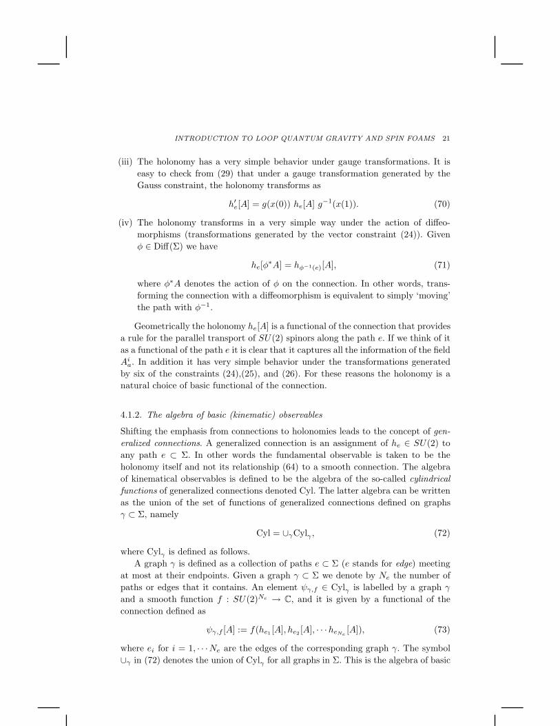
definition. The graph consists of a single closed edge (e = γ) and an example is

shown in Figure 2. Notice, however, that we can also define Wγ [A] as

Wγ [A] := Tr[he1 [A]he2 [A]], (75)

using (68) in which case Wγ [A] ∈ Cylγ′ (γ′ is illustrated in the center of Figure 2).

Moreover, we can also think of Wγ [A] ∈ Cylγ′′ (γ′′ is shown on the right of Figure 2)

as a function of he1 [A] and he2 [A] and he3 [A] (with trivial dependence on the third

argument). There are many ways to represent an element of Cyl as a cylindrical

function on a graph. This flexibility in choosing the graph will be important in the

definition of Hkin and its inner product in the following section.

e e1

e2

e1

e2

e3

Fig. 2. An example of three different graphs on which the Wilson loop function (74) can bedefined. The distinction must be physically irrelevant.

Let us come back to our examples. There is a simple generalization of the previ-

ous gauge invariant function. Given an arbitrary representation matrix M of SU(2),

then clearly WMγ [A] = Tr[M(he[A])] is a gauge invariant cylindrical function. Uni-

tary irreducible representation matrices of spin j will be denoted byj

Πmm′ for

−j ≤ m,m′ ≤ j. The cylindrical function

W jγ [A] := Tr[

j

Π (he[A])] (76)

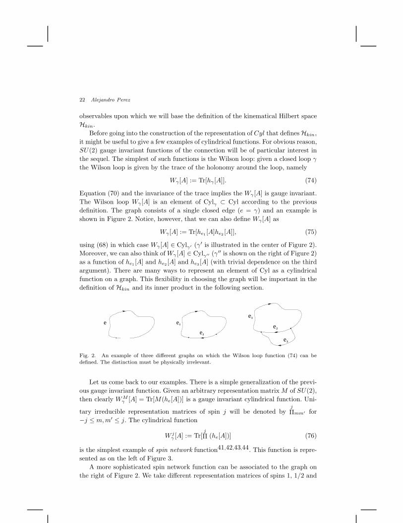
is the simplest example of spin network function41,42,43,44. This function is repre-

sented as on the left of Figure 3.

A more sophisticated spin network function can be associated to the graph on

the right of Figure 2. We take different representation matrices of spins 1, 1/2 and

INTRODUCTION TO LOOP QUANTUM GRAVITY AND SPIN FOAMS 23

j

1/2

1/2

1

j

k

l

Fig. 3. Examples of spin networks.

1/2 evaluate them on the holonomy along e1, e2, and e3 respectively. We define

Θ1,1/2,1/2

e1∪e2∪e3[A] =

1

Π (he1 [A])ij1/2

Π (he2 [A])AB

1/2

Π (he3 [A])CD σACi σBD

j , (77)

where i, j = 1, 2, 3 are vector indices, A,B,C,D = 1, 2 are spinor indices, sum over

repeated indices is understood and σACi are Pauli matrices. It is easy to check that

Θ1,1/2,1/2

e1∪e2∪e3[A] is gauge invariant. This is because the Pauli matrices are invariant

tensors in the tensor product of representations 1⊗ 1/2⊗ 1/2 which is where gauge

transformations act on the nodes of the graph e1 ∪ e2 ∪ e3. Such spin network

function is illustrated on the middle of Figure 3. We can generalize this to arbitrary

representations. Given an invariant tensor ι ∈ j ⊗ k ⊗ l the cylindrical function

Θj,k,l

e1∪e2∪e3[A] =

j

Π (he1 [A])m1n1

k

Π (he2 [A])m2n2

l

Π (he3 [A])m3n3 ιm1m2m3ιn1n2n3 (78)

is gauge invariant by construction. The example is shown on the right of Figure 3.

j

k s

p

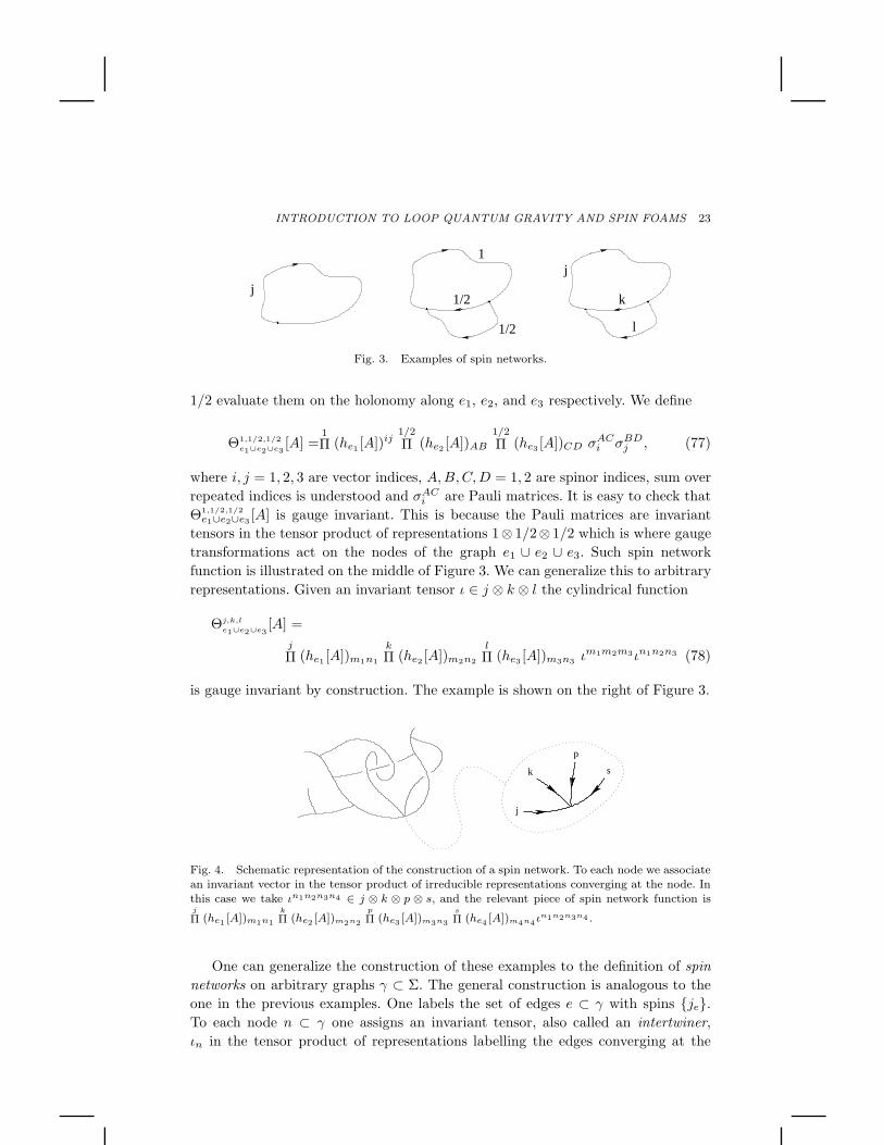
Fig. 4. Schematic representation of the construction of a spin network. To each node we associatean invariant vector in the tensor product of irreducible representations converging at the node. Inthis case we take ιn1n2n3n4 ∈ j ⊗ k ⊗ p ⊗ s, and the relevant piece of spin network function isj

Π (he1 [A])m1n1

k

Π (he2 [A])m2n2

p

Π (he3 [A])m3n3

s

Π (he4 [A])m4n4 ιn1n2n3n4 .

One can generalize the construction of these examples to the definition of spin

networks on arbitrary graphs γ ⊂ Σ. The general construction is analogous to the

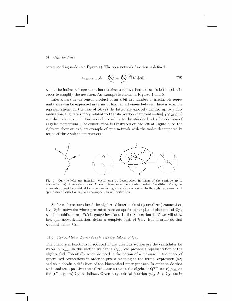
one in the previous examples. One labels the set of edges e ⊂ γ with spins je.To each node n ⊂ γ one assigns an invariant tensor, also called an intertwiner,

ιn in the tensor product of representations labelling the edges converging at the

24 Alejandro Perez

corresponding node (see Figure 4). The spin network function is defined

sγ,je,ιn[A] =⊗

n⊂γ

ιn⊗

e⊂γ

je

Π (he[A]) , (79)

where the indices of representation matrices and invariant tensors is left implicit in

order to simplify the notation. An example is shown in Figures 4 and 5.

Intertwiners in the tensor product of an arbitrary number of irreducible repre-

sentations can be expressed in terms of basic intertwiners between three irreducible

representations. In the case of SU(2) the latter are uniquely defined up to a nor-

malization; they are simply related to Clebsh-Gordon coefficients—Inv[j1 ⊗ j2 ⊗ j3]

is either trivial or one dimensional according to the standard rules for addition of

angular momentum. The construction is illustrated on the left of Figure 5, on the

right we show an explicit example of spin network with the nodes decomposed in

terms of three valent intertwiners..

j

k

s

p

i

12

1

32

25

2

1

1

1

1

1 1

2

1 1

32

12

12

Fig. 5. On the left: any invariant vector can be decomposed in terms of the (unique up tonormalization) three valent ones. At each three node the standard rules of addition of angularmomentum must be satisfied for a non vanishing intertwiner to exist. On the right: an example ofspin network with the explicit decomposition of intertwiners.

So far we have introduced the algebra of functionals of (generalized) connections

Cyl. Spin networks where presented here as special examples of elements of Cyl,

which in addition are SU(2) gauge invariant. In the Subsection 4.1.5 we will show

how spin network functions define a complete basis of Hkin. But in order do that

we must define Hkin.

4.1.3. The Ashtekar-Lewandowski representation of Cyl

The cylindrical functions introduced in the previous section are the candidates for

states in Hkin. In this section we define Hkin and provide a representation of the

algebra Cyl. Essentially what we need is the notion of a measure in the space of

generalized connections in order to give a meaning to the formal expression (62)

and thus obtain a definition of the kinematical inner product. In order to do that

we introduce a positive normalized state (state in the algebraic QFT sense) µAL on

the (C⋆-algebra) Cyl as follows. Given a cylindrical function ψγ,f [A] ∈ Cyl (as in

INTRODUCTION TO LOOP QUANTUM GRAVITY AND SPIN FOAMS 25

(73)) µAL(ψγ,f ) is defined as

µAL(ψγ,f ) =

∫ ∏

e⊂γ

dhe f(he1 , he2 , · · ·heNe), (80)

where he ∈ SU(2) and dh is the (normalized) Haar measure of SU(2) l. The measure

µAL is clearly normalized as µAL(1) = 1 and positive

µAL(ψγ,fψγ,f) =

∫ ∏

e⊂γ

dhe f(he1 , he2 , · · ·heNe)f(he1 , he2 , · · ·heNe

) ≥ 0. (81)

Using the properties of µAL we introduce the inner product

< ψγ,f , ψγ′,g >: = µAL(ψγ,fψγ′,g) =

=

∫ ∏

e⊂Γγγ′

dhe f(he1 , · · ·heNe)g(he1 , · · ·heNe

), (82)

where we use Dirac notation and the cylindrical functions become wave function-

als of the connection corresponding to kinematical states ψγ′,g[A] =< A,ψγ′,g >=

g(he1 , · · ·heNe), and Γγγ′ is any graph such that both γ ⊂ Γγγ′ and γ′ ⊂ Γγγ′.

The state µAL is called the Ashtekar-Lewandowski measure40. The previous equa-

tion is the rigorous definition of (62). The measure µAL—through the GNS

construction45—gives a faithful representation of the algebra of cylindrical func-

tions (i.e., (81) is zero if and only if ψγ,f [A] = 0). The kinematical Hilbert space

Hkin is the Cauchy completion of the space of cylindrical functions Cyl in the

Ashtekar-Lewandowski measure. In other words, in addition to cylindrical func-

tions we add to Hkin the limits of all the Cauchy convergent sequences in the µAL

norm. The operators depending only on the connection act simply by multiplication

in the Ashtekar-Lewandowski representation. This completes the definition of the

kinematical Hilbert space Hkin.

4.1.4. An orthonormal basis of Hkin.

In this section we would like to introduce a very simple basis of Hkin as a prelim-

inary step in the construction of a basis of the Hilbert space of solutions of the

Gauss constraint HG

kin At this stage this is a simple consequence of the Peter-Weyl

theorem46. The Peter-Weyl theorem can be viewed as a generalization of Fourier

theorem for functions on S1. It states that, given a function f ∈ L2[SU(2)], it can

lThe Haar measure of SU(2) is defined by the following properties:

∫

SU(2)dg = 1, and dg = d(αg) = d(gα) = dg−1 ∀α ∈ SU(2).

26 Alejandro Perez

be expressed as a sum over unitary irreducible representations of SU(2), namely m

f(g) =∑

j

√2j + 1 fmm′

j

j

Πmm′ (g), (83)

where

fmm′

j =√

2j + 1

∫

SU(2)

dgj

Πm′m(g−1)f(g), (84)

and dg is the Haar measure of SU(2). This defines the harmonic analysis on SU(2).

The completeness relation

δ(gh−1) =∑

j

(2j + 1)j

Πmm′ (g)j

Πm′m (h−1) =∑

j

(2j + 1)Tr[j

Π (gh−1)], (85)

follows. The previous equations imply the orthogonality relation for unitary repre-

sentations of SU(2)

∫

SU(2)

dg φjm′mφ

j′

q′q = δjj′δmqδm′q′ , (86)

where we have introduce the normalized representation matrices φjmn :=

√2j + 1

j

Πmn for convenience. Given an arbitrary cylindrical function ψγ,f [A] ∈ Cyl

we can use the Peter-Weyl theorem and write

ψγ,f [A] = f(he1 [A], he2 [A], · · ·heNe[A]) =

=∑

j1···jNe

fm1···mNe ,n1···nNe

j1···jNeφj1

m1n1(he1 [A]) · · ·φjNe

mNenNe(heNe

[A]), (87)

where according to (84) fm1···mNe ,n1···nNe

j1···jNeis just given by the kinematical inner

product of the cylindrical function with the tensor product of irreducible represen-

tations, namely (82)

fm1···mNe ,n1···nNe

j1···jNe=< φj1

m1n1· · ·φjNe

mNenNe, ψγ,f >, (88)

where <,> is the kinematical inner product introduced in (82). We have thus

proved that the product of components of (normalized) irreducible representations∏Ne

i=1 φjimini

[hei ] associated with the Ne edges e ⊂ γ (for all values of the spins j

and −j ≤ m,n ≤ j and for any graph γ) is a complete orthonormal basis of Hkin!

mThe link with the U(1) case is direct: for f ∈ L2[U(1)] we have f(θ) =∑

n fn exp(inθ), whereexp(inθ) are unitary irreducible representations of U(1) and fn = (2π)−1

∫dθexp(−inθ)f(θ). The

measure (2π)−1dθ is the Haar measure of U(1).

INTRODUCTION TO LOOP QUANTUM GRAVITY AND SPIN FOAMS 27

4.1.5. Solutions of the Gauss constraint: HG

kin and spin network states

We are now interested in the solutions of the quantum Gauss constraint; the first

three of quantum Einstein’s equations. These solutions are characterized by the

states in Hkin that are SU(2) gauge invariant. These solutions define a new Hilbert

space that we call HG

kin. We leave the subindex kin to keep in mind that there are

still constraints to be solved on the way to Hphys. In previous sections we already

introduced spin network states as natural SU(2) gauge invariant functionals of the

connection42,43,44,47. Now we will show how these are in fact a complete set of

orthogonal solutions of the Gauss constraint, i.e., a basis of HG

kin.

The action of the Gauss constraint is easily represented in Hkin. At this stage

it is simpler to represent finite SU(2) transformations on elements of Hkin (from

which the infinitesimal ones can be easily inferred) using (70). Denoting UG [g] the

operator generating a local g(x) ∈ SU(2) transformation then its action can be

defined directly on the elements of the basis of Hkin defined above, thus

UG [g]φjmn[he] = φj

mn[gsheg−1t ], (89)

where gs is the value of g(x) at the source point of the edge e and gt the value

of g(x) at the target. From the previous equation one can infer the action on an

arbitrary basis element, namely

UG [g]

Ne∏

i=1

φjimini

[hei ] =

Ne∏

i=1

φjimini

[gsiheig−1ti

]. (90)

Now by definition of the scalar product (82) and due to the invariance of the Haar

measure (see Footnote m) the reader can easily prove that UG [g] is a unitary oper-

ator. From the definition it also follows that

UG [g2]UG [g1] = UG [g1g2]. (91)

The projection operator onto the set of states that are solutions of the Gauss con-

straint can be obtained by group averaging techniques. We can denote the projector

PG by

PG =

∫D[g] UG [g], (92)

where the previous expression denotes a formal integration over all SU(2) trans-

formations. Its rigorous definition is given by its action on elements of Cyl. From

equation (89) the operator UG [g] acts on ψγ,g ∈ Cyl at the end points of the edges

e ⊂ γ, and therefore, so does PG. The action of PG on a given (cylindrical) state

ψγ,f ∈ Hkin can therefore be factorized as follows:

PGψγ,f =∏

n⊂γ

PnG ψγ,f , (93)

where PnG acts non trivially only at the node n ⊂ γ. In this way we can define the

action of PG by focusing our attention to a single node n ⊂ γ. For concreteness let

28 Alejandro Perez

us concentrate on the action of PG on an element of ψγ,f ∈ Hkin defined on the

graph illustrated in Figure 4. The state ψγ,f ∈ Hkin admits an expansion in terms

of the basis states as in (87). In particular we concentrate on the action of PG at the

four valent node thereto emphasized, let’s call it n0 ⊂ γ. In order to do that we can

factor out of (87) the (normalized) representation components φjmn corresponding

to that particular node and write

ψγ,f [A] =

=∑

j1···j4

(φj1

m1n1(he1 [A]) · · ·φj4

m4n4(he4 [A])

)× [REST]

m1···m4,n1···n4

j1···j4[A], (94)

where [REST]m1···m4,n1···n4

j1···j4[A] denotes what is left in this factorization, and e1 to

e4 are the four edges converging at n0 (see Figure 4). We can define the meaning of

(92) by giving the action of Pn0

G on φj1m1n1

(he1 [A]) · · ·φj4m4n4

(he4 [A]) as the action on

a general state can be naturally extended from there using (93). Thus we define

Pn0Gφj1

m1n1(he1 [A]) · · ·φj4

m4n4(he4 [A]) =

∫dgφj1

m1n1(ghe1 [A]) · · ·φj4

m4n4(ghe4 [A]), (95)

where dg is the Haar measure of SU(2). Using the fact that

φj1mn(gh[A]) =

j

Πmq (g) φjqn(h[A]) (96)

the action of Pn0

G can be written as

Pn0G φj1

m1n1(he1 [A]) · · ·φj4

m4n4(he4 [A]) =

= Pn0m1···m4,q1···q4

φj1q1n1

(he1 [A]) · · ·φj4q4n4

(he4 [A]), (97)

where

Pn0m1···m4,q1···q4

=

∫dg

j1Πm1q1 (g) · · ·

j4Πm4q4 (g). (98)

If we denote Vj1···j4 the vector space where the representation j1 ⊗· · ·⊗ j4 act, then

previous equation defines a map Pn0 : Vj1···j4 → Vj1···j4 . Using the properties of

the Haar measure given in Footnote m one can show that the map Pn0 is indeed a

projection (i.e., Pn0Pn0 = Pn0). Moreover, we also have

Pn0m1···m4,q1···q4

j1Πq1n1 (g) · · ·

j4Πq4n4 (g) =

=j1Πm1q1 (g) · · ·

j4Πm4q4 (g)Pn0

q1···q4,n1···n4= Pn0

m1···m4,n1···n4, (99)

i.e. Pn0 is right and left invariant. This implies that Pn0 : Vj1···j4 → Inv[Vj1···j4 ],

i.e., the projection from Vj1···j4 onto the (SU(2)) invariant component of the finite

dimensional vector space. We can choose an orthogonal set of invariant vectors

ιαm1···m4(where α labels the elements), in other words an orthonormal basis for

Inv[Vj1···j4 ] and write

Pn0m1···m4,n1···n4

=∑

α

ιαm1···m4ια∗m1···m4

, (100)

INTRODUCTION TO LOOP QUANTUM GRAVITY AND SPIN FOAMS 29

where ∗ denotes the dual basis element. In the same way the action PG on a node

n ⊂ γ of arbitrary valence κ is governed by the corresponding Pn given generally

by

Pnm1···mκ,n1···nκ

=∑

ακ

ιακm1···mκ

ιακ∗m1···mκ

. (101)

According to the tree decomposition of intertwiners in terms of three valent invariant

vectors described around Figure 5, ακ is a (κ− 3)-uple of spins.

Any solution of the Gauss constraint can be written as PGψ for ψ ∈ Hkin. Equa-

tion (93) plus the obvious generalization of (97) for arbitrary nodes implies that the

result of the action of PG on elements of Hkin can be written as a linear combina-

tion of products of representation matrices φjmn contracted with intertwiners, i.e.

spin network states as introduced as examples of elements of Cyl in (79). Spin net-

work states therefore form a complete basis of the Hilbert space of solutions of the

quantum Gauss law HG

kin!

4.2. Geometric operators: quantization of the triad

We have introduced the set of basic configuration observables as the algebra of

cylindrical functions of the generalized connections, and have defined the kinemati-

cal Hilbert space through the Ashtekar-Lewandowski representation. By considering

finite gauge transformations we avoided quantizing the Gauss constraint in the pre-

vious section, avoiding for simplicity, and for the moment, the quantization of the

triad field Eai present in (26). In this section we will quantize the triad field and

will define a set of geometrical operators that lead to the main physical prediction

of LQG: discreteness of geometry eigenvalues.

The triad Eai naturally induces a two form with values in the Lie algebra of

SU(2), namely, Eai ǫabc. In the quantum theory Ea

i becomes an operator valued

distribution. In other words we expect integrals of the triad field with suitable test

functions to be well defined self adjoint operators in Hkin. The two form naturally

associated to Eai suggests that the smearing should be defined on two dimensional

surfaces:

E[S, α] =

∫

S

dσ1dσ2 ∂xa

∂σ1

∂xb

∂σ2αiEa

i ǫabc = −i~κγ∫

S

dσ1dσ2 ∂xa

∂σ1

∂xb

∂σ2αi δ

δAic

ǫabc,

(102)

where αi is a smearing function with values on the Lie algebra of SU(2). The

previous expression corresponds to the natural generalization of the notion of electric

flux operator in electromagnetism. In order to study the action of (102) in Hkin we

notice that

δ

δAic

he[A] =δ

δAic

(P exp

∫ds xd(s)Ak

d τk

)=

=

∫ds xc(s)δ(3)(x(s) − x)he1 [A]τihe2 [A], (103)

30 Alejandro Perez

where he1 [A] and he2 [A] are the holonomy along the two new edges defined by the

point at which the triad acts. Therefore

E[S, α]he[A] =

= −i8πℓ2pγ∫dσ1dσ2dσ3 ∂x

a

∂σ1

∂xb

∂σ2

∂xc

∂sǫabc δ

(3)(x(σ), x(s))αihe1 [A]τihe2 [A]. (104)

Finally using the definition of the delta distribution we obtain a very simple expres-

sion for the action of the flux operator on the holonomy integrating the previous

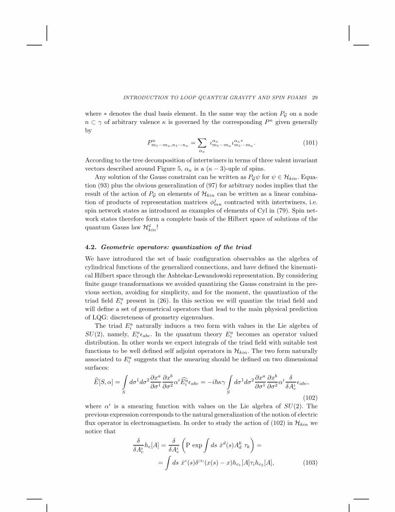
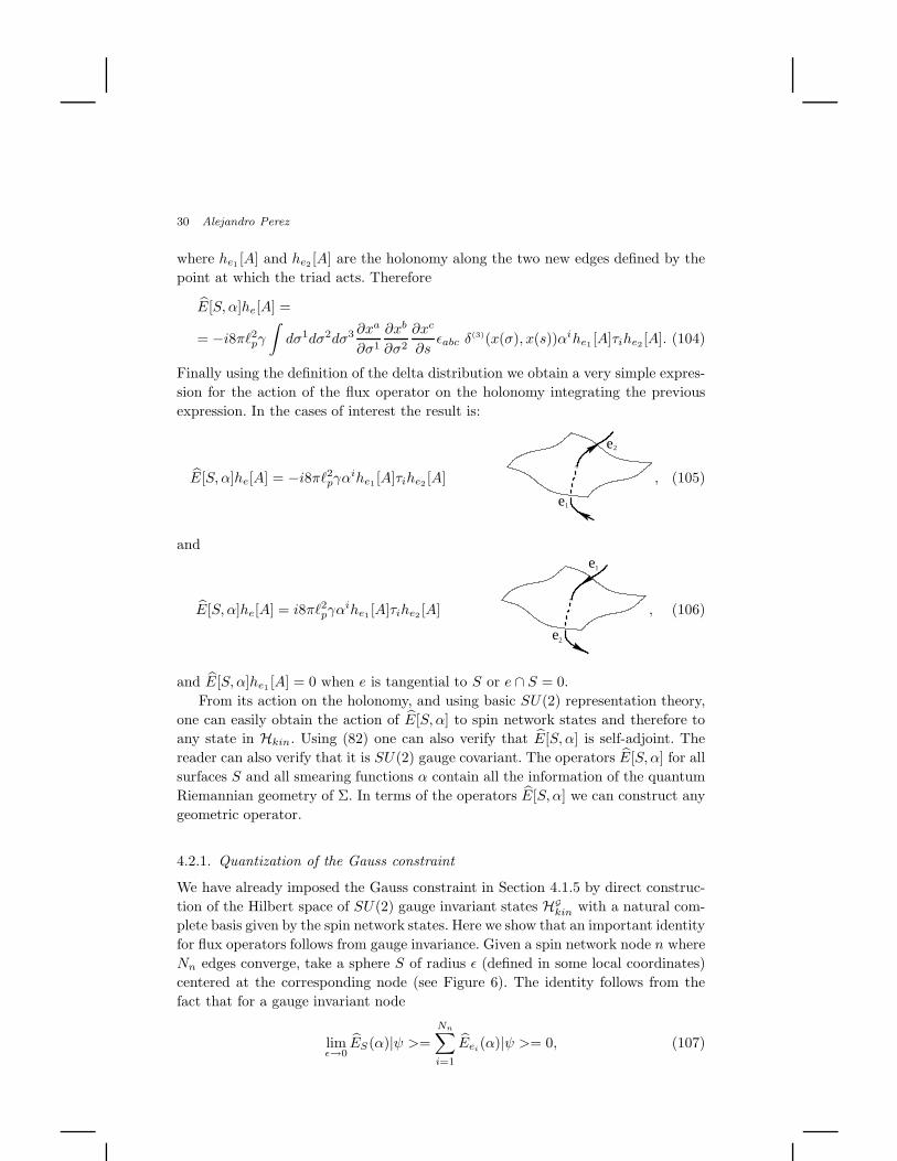
expression. In the cases of interest the result is:

E[S, α]he[A] = −i8πℓ2pγαihe1 [A]τihe2 [A]

e2

e1

, (105)

and

E[S, α]he[A] = i8πℓ2pγαihe1 [A]τihe2 [A]

e2

e1

, (106)

and E[S, α]he1 [A] = 0 when e is tangential to S or e ∩ S = 0.

From its action on the holonomy, and using basic SU(2) representation theory,

one can easily obtain the action of E[S, α] to spin network states and therefore to

any state in Hkin. Using (82) one can also verify that E[S, α] is self-adjoint. The

reader can also verify that it is SU(2) gauge covariant. The operators E[S, α] for all

surfaces S and all smearing functions α contain all the information of the quantum

Riemannian geometry of Σ. In terms of the operators E[S, α] we can construct any

geometric operator.

4.2.1. Quantization of the Gauss constraint

We have already imposed the Gauss constraint in Section 4.1.5 by direct construc-

tion of the Hilbert space of SU(2) gauge invariant states HG

kin with a natural com-

plete basis given by the spin network states. Here we show that an important identity

for flux operators follows from gauge invariance. Given a spin network node n where

Nn edges converge, take a sphere S of radius ǫ (defined in some local coordinates)

centered at the corresponding node (see Figure 6). The identity follows from the

fact that for a gauge invariant node

limǫ→0

ES(α)|ψ >=

Nn∑

i=1

Eei(α)|ψ >= 0, (107)

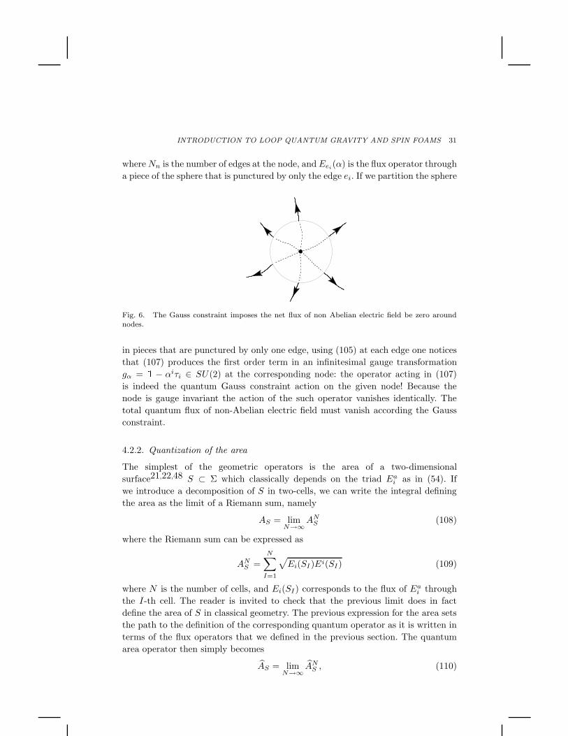
INTRODUCTION TO LOOP QUANTUM GRAVITY AND SPIN FOAMS 31

whereNn is the number of edges at the node, and Eei(α) is the flux operator through

a piece of the sphere that is punctured by only the edge ei. If we partition the sphere

Fig. 6. The Gauss constraint imposes the net flux of non Abelian electric field be zero aroundnodes.

in pieces that are punctured by only one edge, using (105) at each edge one notices

that (107) produces the first order term in an infinitesimal gauge transformation

gα = 1 − αiτi ∈ SU(2) at the corresponding node: the operator acting in (107)

is indeed the quantum Gauss constraint action on the given node! Because the

node is gauge invariant the action of the such operator vanishes identically. The

total quantum flux of non-Abelian electric field must vanish according the Gauss

constraint.

4.2.2. Quantization of the area

The simplest of the geometric operators is the area of a two-dimensional

surface21,22,48 S ⊂ Σ which classically depends on the triad Eai as in (54). If

we introduce a decomposition of S in two-cells, we can write the integral defining

the area as the limit of a Riemann sum, namely

AS = limN→∞

ANS (108)

where the Riemann sum can be expressed as

ANS =

N∑

I=1

√Ei(SI)Ei(SI) (109)

where N is the number of cells, and Ei(SI) corresponds to the flux of Eai through

the I-th cell. The reader is invited to check that the previous limit does in fact

define the area of S in classical geometry. The previous expression for the area sets

the path to the definition of the corresponding quantum operator as it is written in

terms of the flux operators that we defined in the previous section. The quantum

area operator then simply becomes

AS = limN→∞

ANS , (110)

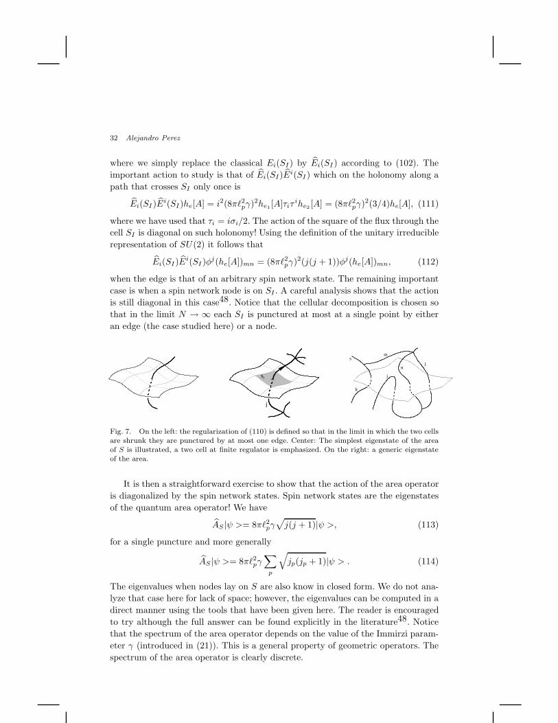
32 Alejandro Perez

where we simply replace the classical Ei(SI) by Ei(SI) according to (102). The

important action to study is that of Ei(SI)Ei(SI) which on the holonomy along a

path that crosses SI only once is

Ei(SI)Ei(SI)he[A] = i2(8πℓ2pγ)

2he1 [A]τiτihe2 [A] = (8πℓ2pγ)

2(3/4)he[A], (111)

where we have used that τi = iσi/2. The action of the square of the flux through the

cell SI is diagonal on such holonomy! Using the definition of the unitary irreducible

representation of SU(2) it follows that

Ei(SI)Ei(SI)φ

j(he[A])mn = (8πℓ2pγ)2(j(j + 1))φj(he[A])mn, (112)

when the edge is that of an arbitrary spin network state. The remaining important

case is when a spin network node is on SI . A careful analysis shows that the action

is still diagonal in this case48. Notice that the cellular decomposition is chosen so

that in the limit N → ∞ each SI is punctured at most at a single point by either

an edge (the case studied here) or a node.

j

sI

k

sm

j

ul

Fig. 7. On the left: the regularization of (110) is defined so that in the limit in which the two cellsare shrunk they are punctured by at most one edge. Center: The simplest eigenstate of the areaof S is illustrated, a two cell at finite regulator is emphasized. On the right: a generic eigenstateof the area.

It is then a straightforward exercise to show that the action of the area operator

is diagonalized by the spin network states. Spin network states are the eigenstates

of the quantum area operator! We have

AS |ψ >= 8πℓ2pγ√j(j + 1)|ψ >, (113)

for a single puncture and more generally

AS |ψ >= 8πℓ2pγ∑

p

√jp(jp + 1)|ψ > . (114)

The eigenvalues when nodes lay on S are also know in closed form. We do not ana-

lyze that case here for lack of space; however, the eigenvalues can be computed in a

direct manner using the tools that have been given here. The reader is encouraged

to try although the full answer can be found explicitly in the literature48. Notice

that the spectrum of the area operator depends on the value of the Immirzi param-

eter γ (introduced in (21)). This is a general property of geometric operators. The

spectrum of the area operator is clearly discrete.

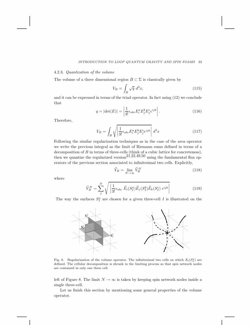
INTRODUCTION TO LOOP QUANTUM GRAVITY AND SPIN FOAMS 33

4.2.3. Quantization of the volume

The volume of a three dimensional region B ⊂ Σ is classically given by

VB =

∫

B

√q d3x, (115)

and it can be expressed in terms of the triad operator. In fact using (12) we conclude

that

q = |det(E)| =

∣∣∣∣1

3!ǫabcE

ai E

bjE

cj ǫ

ijk

∣∣∣∣ . (116)

Therefore,

VB =

∫

B

√∣∣∣∣1

3!ǫabcEa

i EbjE

cj ǫ

ijk

∣∣∣∣ d3x (117)

Following the similar regularization techniques as in the case of the area operator

we write the previous integral as the limit of Riemann sums defined in terms of a

decomposition of B in terms of three-cells (think of a cubic lattice for concreteness),

then we quantize the regularized version21,22,49,50 using the fundamental flux op-

erators of the previous section associated to infinitesimal two cells. Explicitly,

VB = limN→∞

V NB (118)

where

V NB =

N∑

I

√ ∣∣∣∣1

3!ǫabc Ei(Sa

I )Ej(SbI)Ek(Sc

I) ǫijk

∣∣∣∣ (119)

The way the surfaces SaI are chosen for a given three-cell I is illustrated on the

s I2

s1I

s3I

Fig. 8. Regularization of the volume operator. The infinitesimal two cells on which Ei(SaI) are

defined. The cellular decomposition is shrunk in the limiting process so that spin network nodesare contained in only one three cell.

left of Figure 8. The limit N → ∞ is taken by keeping spin network nodes inside a

single three-cell.

Let us finish this section by mentioning some general properties of the volume

operator.

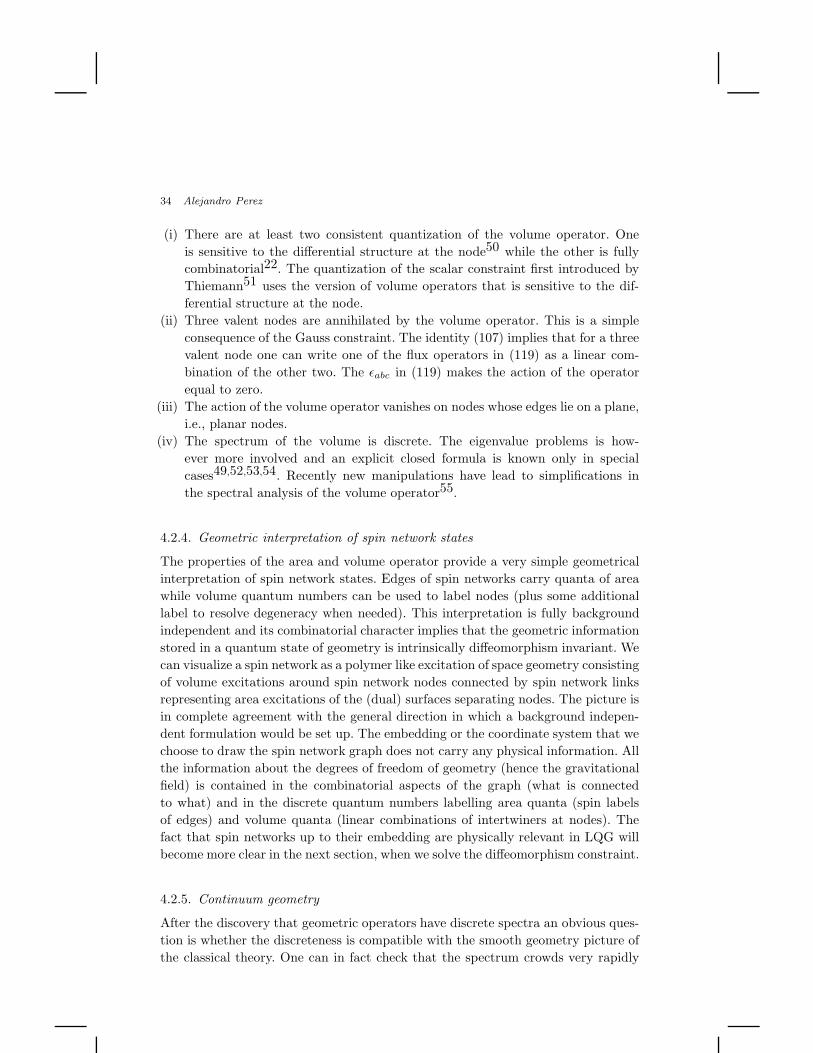
34 Alejandro Perez

(i) There are at least two consistent quantization of the volume operator. One

is sensitive to the differential structure at the node50 while the other is fully

combinatorial22. The quantization of the scalar constraint first introduced by

Thiemann51 uses the version of volume operators that is sensitive to the dif-

ferential structure at the node.

(ii) Three valent nodes are annihilated by the volume operator. This is a simple

consequence of the Gauss constraint. The identity (107) implies that for a three

valent node one can write one of the flux operators in (119) as a linear com-

bination of the other two. The ǫabc in (119) makes the action of the operator

equal to zero.

(iii) The action of the volume operator vanishes on nodes whose edges lie on a plane,

i.e., planar nodes.

(iv) The spectrum of the volume is discrete. The eigenvalue problems is how-

ever more involved and an explicit closed formula is known only in special

cases49,52,53,54. Recently new manipulations have lead to simplifications in

the spectral analysis of the volume operator55.

4.2.4. Geometric interpretation of spin network states

The properties of the area and volume operator provide a very simple geometrical

interpretation of spin network states. Edges of spin networks carry quanta of area

while volume quantum numbers can be used to label nodes (plus some additional

label to resolve degeneracy when needed). This interpretation is fully background

independent and its combinatorial character implies that the geometric information

stored in a quantum state of geometry is intrinsically diffeomorphism invariant. We

can visualize a spin network as a polymer like excitation of space geometry consisting

of volume excitations around spin network nodes connected by spin network links

representing area excitations of the (dual) surfaces separating nodes. The picture is

in complete agreement with the general direction in which a background indepen-

dent formulation would be set up. The embedding or the coordinate system that we

choose to draw the spin network graph does not carry any physical information. All

the information about the degrees of freedom of geometry (hence the gravitational

field) is contained in the combinatorial aspects of the graph (what is connected

to what) and in the discrete quantum numbers labelling area quanta (spin labels

of edges) and volume quanta (linear combinations of intertwiners at nodes). The

fact that spin networks up to their embedding are physically relevant in LQG will

become more clear in the next section, when we solve the diffeomorphism constraint.

4.2.5. Continuum geometry

After the discovery that geometric operators have discrete spectra an obvious ques-

tion is whether the discreteness is compatible with the smooth geometry picture of

the classical theory. One can in fact check that the spectrum crowds very rapidly

INTRODUCTION TO LOOP QUANTUM GRAVITY AND SPIN FOAMS 35

when one gets to larger geometries as the spacing between eigenvalues decreases

exponentially for large eigenvalues.

4.3. Solutions of the diffeomorphism constraint: HD

kinand abstract

spin networks

In Section 4.1.5 we solved the three quantum Einstein’s equations defining the

Hilbert space of SU(2) gauge invariant states given by HG

kin ⊂ Hkin. Now we turn

our attention to the next three quantum constraint equations, the vector constraint

(24). The technique that we apply to find the Hilbert space of diffeomorphism

invariant states HD

kin is analogous to the one used to obtain HG

kin. However, because

the orbits of the diffeomorphisms are not compact, diffeomorphism invariant states

are not contained in the original Hkin. In relation to Hkin, they have to be regarded

as distributional states40.

A simple example will allow us to introduce the basic ideas. Consider an ordinary

particle quantum system defined on a cylinder. Assume the kinematical Hilbert

space is given by square integrable functions ψ(θ, z) or Hkin = L2(S1 × R). In

addition assume one has to solve the following constraint equations:

pθψ = 0 and pzψ = 0. (120)

The first constraint generates rotations around the z-axis, i.e. it has compact orbits,

and, in this sense, is the analog of the Gauss constraint in LQG. The solutions of

the first constraint are wave functions invariant under rotations around z, those

that do not depend on θ. Therefore they are contained in the original Hilbert space

Hkin because, as the orbits of pθ are compact, square integrable functions ψ(z) (i.e.,

independent of θ) exist. The second constraint has non compact orbits and in this

sense is the analog of the diffeomorphism constraint in LQG. The solution of the

second constraint are functions that do not depend on z. They cannot be contained

in Hkin, as functions ψ(θ) cannot be in Hkin = L2(S1×R). However given a suitable

dense subset of Φ ⊂ Hkin of test functions, e.g. functions of compact support, then

any solution of the latter constraint can be given a meaning as a distribution. For

instance a solution of both constraints does not depend neither on θ nor on z. Its

wave function corresponds to a constant (ψ0|θ, z >= c . The solution (ψ0| is clearly

not in Hkin. We use a rounded brackets in the notation to recall this fact. (ψ0| is

in Φ⋆, the topological dual of Φ, i.e., the set of linear functionals from Φ to C. Its

action on any arbitrary function of compact support |α >∈ Φ ⊂ Hkin is given by

(ψ0|α >=

∫dz dθ c α(θ, z), (121)

which is well defined. The action of (ψ0| extracts the gauge invariant information

from the non gauge invariant state |α >. As vector spaces we have the relation Φ ⊂Hkin ⊂ Φ⋆, usually called the Gelfand triple. In the case of LQG diffeomorphism

invariant states are in the dual of the cylindrical functions Cyl. The Gelfand triple of

36 Alejandro Perez

interest is Cyl ⊂ Hkin ⊂ Cyl⋆. Diffeomorphism invariant states have a well defined

meaning as linear forms in Cyl⋆.

Let us now apply the same idea to define diffeomorphism invariant states. Dif-

feomorphism transformations are easily represented in Hkin. We denote UD[φ] the

operator representing the action of a diffeomorphism φ ∈ Diff(Σ). Its action can

be defined directly on the dense subset of cylindrical functions Cyl ⊂ Hkin. Given

ψγ,f ∈ Cyl as in (73) we have

UD[φ]ψγ,f [A] = ψφ−1γ,f [A], (122)

which naturally follows from (71). Diffeomorphisms act on elements of Cyl (such as

spin networks) by simply modifying the underlying graph in the obvious manner.

Notice that UD[φ] is unitary according to the definition (82).

Notice that because (122) is not weakly continuous there is no well defined

notion of self-adjoint generator of infinitesimal diffeomorphisms in Hkinn. In other

words the unitary operator that implements a diffeomorphism transformation is well

defined but there is no corresponding self adjoint operator whose exponentiation

leads to UD[φ]. Therefore, the diffeomorphism constraint cannot be quantized in

the Ashtekar-Lewandowski representation. This is not really a problem as UD[φ] is

all we need in the quantum theory to look for diffeomorphism invariant states. In

LQG one replaces the second set of formal equations in (63) by the well defined

equivalent requirement

UD[φ]ψ = ψ (123)

for (distributional states) ψ ∈ Cyl⋆.

We are now ready to explicitly write the solutions, namely

([ψγ,f ]| =∑

φ∈Diff(Σ)

< ψγ,f |UD[φ] =∑

φ∈Diff(Σ)

< ψφγ,f |, (124)

were the sum is over all diffeomorphisms. The brackets in ([ψγ,f ]| denote that the

distributional state depends only on the equivalence class [ψγ,f ] under diffeomor-

phisms. Clearly we have ([ψγ,f ]|UD[α] = ([ψγ,f ]| for any α ∈ Diff(Σ). Now we need

to check that ([ψγ,f ]| ∈ Cyl⋆ so that the huge sum in (124) gives a finite result when

applied to an element |ψγ′,g >∈ Cyl, i.e., it is a well defined linear form. That this

is the case follows from (82) (see the remark in Footnote n) as in

([ψγ,f ]|ψγ′,g > (125)

only a finite number of terms from (124) contribute. In fact for spin networks with

no discrete symmetries there is only one non trivial contribution.

The action of ([ψγ,f ]| is diffeomorphism invariant, namely

([ψγ,f ]|ψγ′,g >= ([ψγ,f ]|UD[φ]ψγ′,g > (126)

n This is because for any φ ∈ Diff(Σ) the state UD [φ]ψ is orthogonal to ψ for a generic ψ ∈ Hkin.

INTRODUCTION TO LOOP QUANTUM GRAVITY AND SPIN FOAMS 37

The inner product < , >diff needed to promote the set of diffeomorphism invariant

states to the Hilbert space HD

kin is defined as

< [ψγ,f ]|[ψγ′,g] >diff= ([ψγ,f ]|ψγ′,g > (127)

Due to (126) the previous equation is well defined among diffeomorphism equiva-

lence classes of states under the action of diffeomorphisms and hence this is denoted

by the brackets on both sides.

4.3.1. The quantization of the scalar constraint

In this section we sketch the regularization and definition of the last constraint to

be quantized and solved: the scalar constraint. The smeared version of the classical

scalar constraint is

S(N) =

∫

Σ

dx3 NEa

i Ebj√

det(E)

(ǫijkF

kab − 2(1 + γ2)Ki

[aKjb]

)=

= SE(N) − 2(1 + γ2) T (N), (128)

where Kia = γ−1(Ai

a − Γia), and in the second line we have introduced a convenient

separation of the constraint into what is called the Euclidean contribution SE(N)

given by

SE(N) =

∫

Σ

dx3 NEa

i Ebj√

det(E)ǫijkF

kab, (129)

and the extra piece

T (N) =

∫

Σ

dx3 NEa

i Ebj√

det(E)Ki

[aKjb]. (130)

The terms in the constraint look in fact very complicated. On the one hand they

are highly non linear which anticipates difficulties in the quantization related to

regularization issues and potential UV divergences, factor ordering ambiguities, etc.

For instance the factor 1/det(E) looks quite complicated at first sight as does the

spin connection Γia in the expression of Ki

a (recall its definition (19) and (20) in

terms of the basic triad variables).

The crucial simplification of the apparently intractable problem came from the

ideas of Thiemann56. He observed that if one introduces the phase space functional

K :=

∫

Σ

KiaE

ai , (131)

then the following series of identities hold:

Kia = γ−1(Ai

a − Γia) =

1

κγ

Ai

a, K, (132)

38 Alejandro Perez

K =1

γ3/2

SE(1), V

, (133)

where V =∫ √

det(E) is the volume of Σ, and finally

EbiE

cj√

det(E)ǫijkǫabc =

4

κγ

Ak

a, V. (134)

With all this we can write the terms in the scalar constraint by means of Poisson

brackets among quantities that are simple enough to consider their quantization.

The Euclidean constraint can be written as

SE(N) =

∫

Σ

dx3 N ǫabcδijFiab

Aj

c, V, (135)

while the term T (N) becomes

T (N) =

∫

Σ

dx3 N

κ2γ3ǫabcǫijk

Ai

a,SE(1), V

Aj

b,SE(1), V

Ak

c , V. (136)

The new form suggests that we can quantize the constraint by promoting the ar-

gument of the Poisson brackets to operators and the Poisson brackets them self

to commutators in the standard way. One needs the volume operator V , whose

quantization was already discussed, and the quantization of the connection and

curvature. We present here the basic idea behind the quantization of these. For a

precise treatment the reader is encouraged to read Thiemann’s original work51,57

and book20. Given an infinitesimal loop αab on the ab-plane with coordinate area

ǫ2, the curvature tensor can be regularized observing that

hαab[A] − h−1

αab[A] = ǫ2F i

abτi + O(ǫ4). (137)

Similarly the Poisson bracketAi

a, V

is regularized as

h−1ea

[A] hea [A], V = ǫAi

a, V

+ O(ǫ2), (138)

where ea is a path along the a-coordinate of coordinate length ǫ. With this we can

write

SE(N) =

= limǫ→0

∑

I

NIǫ3 ǫabcTr [Fab(A) Ac, V ] =

= limǫ→0

∑

I

NI ǫabcTr

[(hαI

ab[A] − h−1

αIab

[A])h−1eI

c[A]

heI

c[A], V

], (139)

where in the first equality we have replaced the integral (135) by a Riemann sum

over cells of coordinate volume ǫ3 and in the second line we have written it in

terms of holonomies. Notice that the explicit dependence on the cell size ǫ has

disappeared in the last line. The cells are labelled with the index I in analogy to

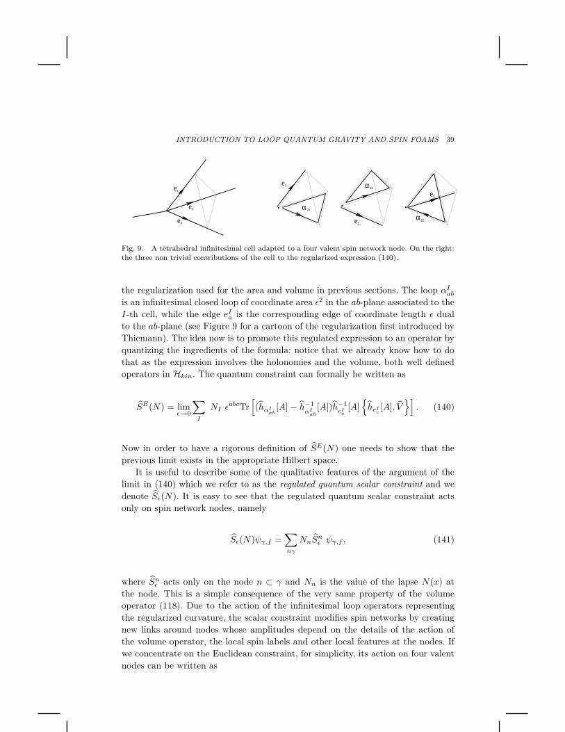
INTRODUCTION TO LOOP QUANTUM GRAVITY AND SPIN FOAMS 39

e1

e2

e3

1e

23α

2e

α 31

α 12

e3

Fig. 9. A tetrahedral infinitesimal cell adapted to a four valent spin network node. On the right:the three non trivial contributions of the cell to the regularized expression (140).

the regularization used for the area and volume in previous sections. The loop αIab

is an infinitesimal closed loop of coordinate area ǫ2 in the ab-plane associated to the

I-th cell, while the edge eIa is the corresponding edge of coordinate length ǫ dual

to the ab-plane (see Figure 9 for a cartoon of the regularization first introduced by

Thiemann). The idea now is to promote this regulated expression to an operator by

quantizing the ingredients of the formula: notice that we already know how to do

that as the expression involves the holonomies and the volume, both well defined

operators in Hkin. The quantum constraint can formally be written as

SE(N) = limǫ→0

∑

I

NI ǫabcTr

[(hαI

ab[A] − h−1

αIab

[A])h−1eI

c[A]

heI

c[A], V

]. (140)

Now in order to have a rigorous definition of SE(N) one needs to show that the

previous limit exists in the appropriate Hilbert space.

It is useful to describe some of the qualitative features of the argument of the

limit in (140) which we refer to as the regulated quantum scalar constraint and we

denote Sǫ(N). It is easy to see that the regulated quantum scalar constraint acts

only on spin network nodes, namely

Sǫ(N)ψγ,f =∑

nγ

NnSnǫ ψγ,f , (141)

where Snǫ acts only on the node n ⊂ γ and Nn is the value of the lapse N(x) at

the node. This is a simple consequence of the very same property of the volume

operator (118). Due to the action of the infinitesimal loop operators representing

the regularized curvature, the scalar constraint modifies spin networks by creating

new links around nodes whose amplitudes depend on the details of the action of

the volume operator, the local spin labels and other local features at the nodes. If

we concentrate on the Euclidean constraint, for simplicity, its action on four valent

nodes can be written as

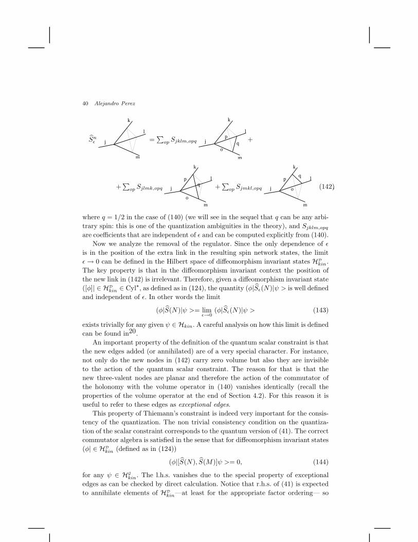
40 Alejandro Perez

Snǫ j

k

l

m

=∑

op Sjklm,opq

o

pl

qj

m

k

+

+∑

op Sjlmk,opq

l

j

m

k

p

o

q +∑

op Sjmkl,opq

l

j

m

k

pq

o ,(142)

where q = 1/2 in the case of (140) (we will see in the sequel that q can be any arbi-

trary spin: this is one of the quantization ambiguities in the theory), and Sjklm,opq

are coefficients that are independent of ǫ and can be computed explicitly from (140).

Now we analyze the removal of the regulator. Since the only dependence of ǫ

is in the position of the extra link in the resulting spin network states, the limit

ǫ→ 0 can be defined in the Hilbert space of diffeomorphism invariant states HD

kin.

The key property is that in the diffeomorphism invariant context the position of

the new link in (142) is irrelevant. Therefore, given a diffeomorphism invariant state

([φ]| ∈ HD

kin ∈ Cyl⋆, as defined as in (124), the quantity (φ|Sǫ(N)|ψ > is well defined

and independent of ǫ. In other words the limit

(φ|S(N)|ψ >= limǫ→0

(φ|Sǫ(N)|ψ > (143)

exists trivially for any given ψ ∈ Hkin. A careful analysis on how this limit is defined

can be found in20.

An important property of the definition of the quantum scalar constraint is that

the new edges added (or annihilated) are of a very special character. For instance,

not only do the new nodes in (142) carry zero volume but also they are invisible

to the action of the quantum scalar constraint. The reason for that is that the

new three-valent nodes are planar and therefore the action of the commutator of

the holonomy with the volume operator in (140) vanishes identically (recall the

properties of the volume operator at the end of Section 4.2). For this reason it is

useful to refer to these edges as exceptional edges.

This property of Thiemann’s constraint is indeed very important for the consis-

tency of the quantization. The non trivial consistency condition on the quantiza-

tion of the scalar constraint corresponds to the quantum version of (41). The correct

commutator algebra is satisfied in the sense that for diffeomorphism invariant states

(φ| ∈ HD

kin (defined as in (124))

(φ|[S(N), S(M)]ψ >= 0, (144)

for any ψ ∈ HG

kin. The l.h.s. vanishes due to the special property of exceptional

edges as can be checked by direct calculation. Notice that r.h.s. of (41) is expected

to annihilate elements of HD

kin—at least for the appropriate factor ordering— so

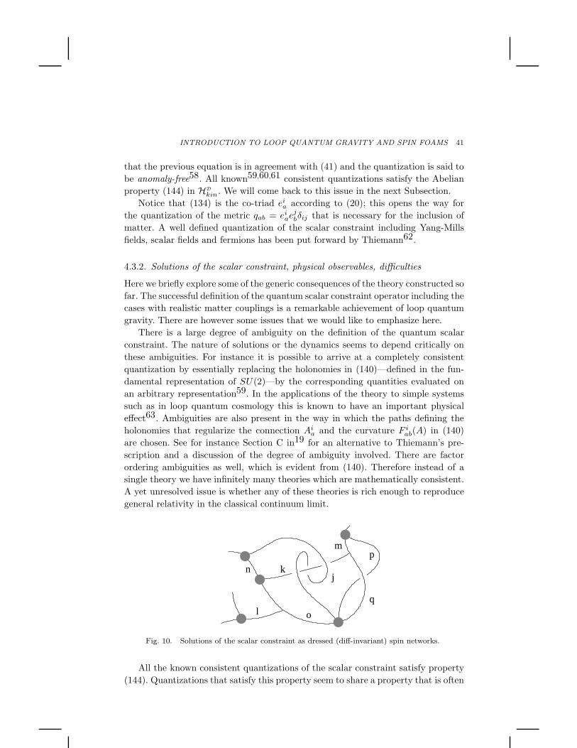
INTRODUCTION TO LOOP QUANTUM GRAVITY AND SPIN FOAMS 41

that the previous equation is in agreement with (41) and the quantization is said to

be anomaly-free58. All known59,60,61 consistent quantizations satisfy the Abelian

property (144) in HD

kin. We will come back to this issue in the next Subsection.

Notice that (134) is the co-triad eia according to (20); this opens the way for

the quantization of the metric qab = eiae

jbδij that is necessary for the inclusion of

matter. A well defined quantization of the scalar constraint including Yang-Mills

fields, scalar fields and fermions has been put forward by Thiemann62.

4.3.2. Solutions of the scalar constraint, physical observables, difficulties

Here we briefly explore some of the generic consequences of the theory constructed so

far. The successful definition of the quantum scalar constraint operator including the

cases with realistic matter couplings is a remarkable achievement of loop quantum

gravity. There are however some issues that we would like to emphasize here.

There is a large degree of ambiguity on the definition of the quantum scalar

constraint. The nature of solutions or the dynamics seems to depend critically on

these ambiguities. For instance it is possible to arrive at a completely consistent

quantization by essentially replacing the holonomies in (140)—defined in the fun-

damental representation of SU(2)—by the corresponding quantities evaluated on

an arbitrary representation59. In the applications of the theory to simple systems

such as in loop quantum cosmology this is known to have an important physical

effect63. Ambiguities are also present in the way in which the paths defining the

holonomies that regularize the connection Aia and the curvature F i

ab(A) in (140)

are chosen. See for instance Section C in19 for an alternative to Thiemann’s pre-

scription and a discussion of the degree of ambiguity involved. There are factor

ordering ambiguities as well, which is evident from (140). Therefore instead of a

single theory we have infinitely many theories which are mathematically consistent.

A yet unresolved issue is whether any of these theories is rich enough to reproduce

general relativity in the classical continuum limit.

l

n kj

o

pm

q

Fig. 10. Solutions of the scalar constraint as dressed (diff-invariant) spin networks.

All the known consistent quantizations of the scalar constraint satisfy property

(144). Quantizations that satisfy this property seem to share a property that is often

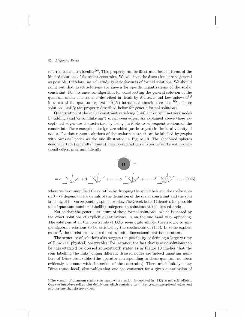
42 Alejandro Perez

referred to as ultra-locality64. This property can be illustrated best in terms of the

kind of solutions of the scalar constraint. We will keep the discussion here as general

as possible; therefore, we will study generic features of formal solutions. We should

point out that exact solutions are known for specific quantizations of the scalar

constraint. For instance, an algorithm for constructing the general solution of the

quantum scalar constraint is described in detail by Ashtekar and Lewandowski19

in terms of the quantum operator S(N) introduced therein (see also 65). These

solutions satisfy the property described below for generic formal solutions.

Quantization of the scalar constraint satisfying (144) act on spin network nodes

by adding (and/or annihilatingo) exceptional edges. As explained above these ex-

ceptional edges are characterized by being invisible to subsequent actions of the

constraint. These exceptional edges are added (or destroyed) in the local vicinity of

nodes. For that reason, solutions of the scalar constraint can be labelled by graphs

with ‘dressed’ nodes as the one illustrated in Figure 10. The shadowed spheres

denote certain (generally infinite) linear combinations of spin networks with excep-

tional edges, diagrammatically

ΟΩ =

= α + β + · · · + γ + · · · + δ + · · · ,(145)

where we have simplified the notation by dropping the spin labels and the coefficients

α, β · · · δ depend on the details of the definition of the scalar constraint and the spin

labelling of the corresponding spin networks. The Greek letter Ω denotes the possible

set of quantum numbers labelling independent solutions at the dressed nodes.

Notice that the generic structure of these formal solutions—which is shared by

the exact solutions of explicit quantizations—is on the one hand very appealing.

The solutions of all the constraints of LQG seem quite simple: they reduce to sim-

ple algebraic relations to be satisfied by the coefficients of (145). In some explicit

cases19, these relations even reduced to finite dimensional matrix operations.

The structure of solutions also suggest the possibility of defining a large variety

of Dirac (i.e. physical) observables. For instance, the fact that generic solutions can

be characterized by dressed spin-network states as in Figure 10 implies that the

spin labelling the links joining different dressed nodes are indeed quantum num-

bers of Dirac observables (the operator corresponding to these quantum numbers

evidently commute with the action of the constraint). There are infinitely many

Dirac (quasi-local) observables that one can construct for a given quantization of

oThe version of quantum scalar constraint whose action is depicted in (142) is not self adjoint.One can introduce self adjoint definitions which contain a term that creates exceptional edges andanother one that destroys them.

INTRODUCTION TO LOOP QUANTUM GRAVITY AND SPIN FOAMS 43

the scalar constraint satisfying (144)p. However, at present it is not very clear what

the physical interpretation of these observables would be.

On the other hand, the ultra-local character of the solutions has raised some

concerns of whether the quantum theories of the Thiemann type can reproduce the

physics of gravity in the classical limit64. In order to illustrate this point let us go

back to the classical theory. Since at the classical level we can invert the transfor-

mations that lead to new variables in Section 2 let us work with the constraints in

ADM variables. We simplify the discussion by considering the York-Lichnerowicz

conformal decompositions for initial data. For the discussion here we can specialize

to the time-symmetric case Kab = 0 and we take the ansatz qab = ψ4q0ab for some

given q0ab defined up to a conformal factor. The vector constraint is in this case

identically zero and the only non trivial constraint is the scalar constraint that can

be shown to be

∆0ψ − 1

8R(q0) = 0, (146)

where ∆0 is the covariant Laplacian defined with respect to q0ab. The point is that

the previous equation is manifestly elliptic which is a general property of the scalar

constraint written in this form67. This means that if we give the value of ψ on a

sphere, the scalar constraint (146) will determine the value of ψ inside. The scalar

constraint in general relativity imposes a condition among unphysical degrees of

freedom (represented by ψ in this case) that “propagate” along the initial value

surfaceq. The only point in writing the initial value problem in this way is to em-

phasize this property of the scalar constraint.

Coming back to the quantum theory one can construct semi-classical states by

taking linear combinations of kinematical spin-network states in order to approx-

imate some classical geometry qab68,69. In that context one could define a sphere

with some given semi-classical area. Now because the scalar constraint acts only in

the immediate vicinity of nodes and does not change the value of the spins of the

edges that connect different dressed nodes it is not clear how the elliptic character

of the classical scalar constraint would be recovered in this semi-classical context. In

other words, how is it that quantizations of the scalar constraint that are ultra-local

in the sense above can impose conditions restricting unphysical degrees of freedom

in the interior of the sphere once boundary conditions defining the geometry of the

pThe intuitive idea here is presented in terms of a given solution of the constraint based on a givenfamily of graphs: the dressed spin-networks. One should keep in mind that defining a quantumoperators representing a Dirac observable implies defining its action on the whole Hphys. A simpleexample of Dirac operator whose action is defined far all solutions is for instance OD =

∑e je,

i.e., the sum of the spins connecting dressed nodes66.qWith the time-symmetric ansatz Kab = 0 for the five degrees of freedom in the conformal metricq0ab

only one local physical degree of freedom remains after factoring out the action of the con-straints as generating functions of gauge transformations. In this context our truncation leads toonly one free data per space-point. Despite these restrictions there are many radiating spacetimesand other interesting solutions in this sector.

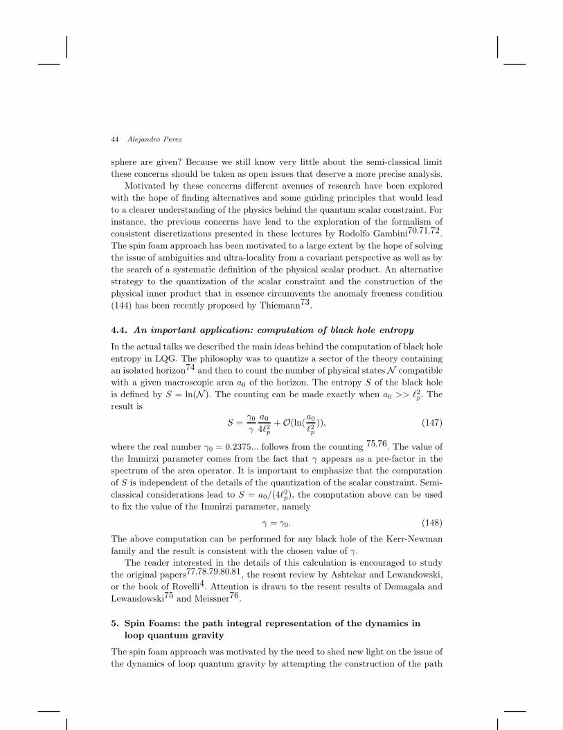
44 Alejandro Perez

sphere are given? Because we still know very little about the semi-classical limit

these concerns should be taken as open issues that deserve a more precise analysis.

Motivated by these concerns different avenues of research have been explored

with the hope of finding alternatives and some guiding principles that would lead

to a clearer understanding of the physics behind the quantum scalar constraint. For

instance, the previous concerns have lead to the exploration of the formalism of

consistent discretizations presented in these lectures by Rodolfo Gambini70,71,72.

The spin foam approach has been motivated to a large extent by the hope of solving

the issue of ambiguities and ultra-locality from a covariant perspective as well as by

the search of a systematic definition of the physical scalar product. An alternative

strategy to the quantization of the scalar constraint and the construction of the

physical inner product that in essence circumvents the anomaly freeness condition

(144) has been recently proposed by Thiemann73.

4.4. An important application: computation of black hole entropy

In the actual talks we described the main ideas behind the computation of black hole

entropy in LQG. The philosophy was to quantize a sector of the theory containing

an isolated horizon74 and then to count the number of physical states N compatible

with a given macroscopic area a0 of the horizon. The entropy S of the black hole

is defined by S = ln(N ). The counting can be made exactly when a0 >> ℓ2p. The

result is

S =γ0

γ

a0

4ℓ2p+ O(ln(

a0

ℓ2p)), (147)

where the real number γ0 = 0.2375... follows from the counting 75,76. The value of

the Immirzi parameter comes from the fact that γ appears as a pre-factor in the

spectrum of the area operator. It is important to emphasize that the computation

of S is independent of the details of the quantization of the scalar constraint. Semi-

classical considerations lead to S = a0/(4ℓ2p), the computation above can be used

to fix the value of the Immirzi parameter, namely

γ = γ0. (148)

The above computation can be performed for any black hole of the Kerr-Newman

family and the result is consistent with the chosen value of γ.

The reader interested in the details of this calculation is encouraged to study

the original papers77,78,79,80,81, the resent review by Ashtekar and Lewandowski,

or the book of Rovelli4. Attention is drawn to the resent results of Domagala and

Lewandowski75 and Meissner76.

5. Spin Foams: the path integral representation of the dynamics in

loop quantum gravity

The spin foam approach was motivated by the need to shed new light on the issue of

the dynamics of loop quantum gravity by attempting the construction of the path

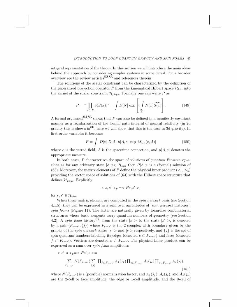
INTRODUCTION TO LOOP QUANTUM GRAVITY AND SPIN FOAMS 45

integral representation of the theory. In this section we will introduce the main ideas

behind the approach by considering simpler systems in some detail. For a broader

overview see the review articles82,83 and references therein.

The solutions of the scalar constraint can be characterized by the definition of

the generalized projection operator P from the kinematical Hilbert space Hkin into

the kernel of the scalar constraint Hphys. Formally one can write P as

P = “∏

x⊂ Σ

δ(S(x))” =

∫D[N ] exp

i∫

Σ

N(x)S(x)

. (149)

A formal argument84,85 shows that P can also be defined in a manifestly covariant

manner as a regularization of the formal path integral of general relativity (in 2d

gravity this is shown in86, here we will show that this is the case in 3d gravity). In

first order variables it becomes

P =

∫D[e] D[A] µ[A, e] exp [iSGR(e,A)] (150)

where e is the tetrad field, A is the spacetime connection, and µ[A, e] denotes the

appropriate measure.

In both cases, P characterizes the space of solutions of quantum Einstein equa-

tions as for any arbitrary state |φ >∈ Hkin then P |φ > is a (formal) solution of

(63). Moreover, the matrix elements of P define the physical inner product (< , >p)

providing the vector space of solutions of (63) with the Hilbert space structure that

defines Hphys. Explicitly

< s, s′ >p:=< Ps, s′ >,

for s, s′ ∈ Hkin.

When these matrix element are computed in the spin network basis (see Section

4.1.5), they can be expressed as a sum over amplitudes of ‘spin network histories’:

spin foams (Figure 11). The latter are naturally given by foam-like combinatorial

structures whose basic elements carry quantum numbers of geometry (see Section

4.2). A spin foam history87, from the state |s > to the state |s′ >, is denoted

by a pair (Fs→s′ , j) where Fs→s′ is the 2-complex with boundary given by the

graphs of the spin network states |s′ > and |s > respectively, and j is the set of

spin quantum numbers labelling its edges (denoted e ⊂ Fs→s′) and faces (denoted

f ⊂ Fs→s′ ). Vertices are denoted v ⊂ Fs→s′ . The physical inner product can be

expressed as a sum over spin foam amplitudes

< s′, s >p=< Ps′, s >=

∑Fs→s′

N(Fs→s′ )∑j

∏f⊂Fs→s′

Af (jf )∏

e⊂Fs→s′Ae(je)

∏v⊂Fs→s′

Av(jv),

(151)

where N(Fs→s′ ) is a (possible) normalization factor, and Af (jf ), Ae(je), and Av(jv)

are the 2-cell or face amplitude, the edge or 1-cell amplitude, and the 0-cell of

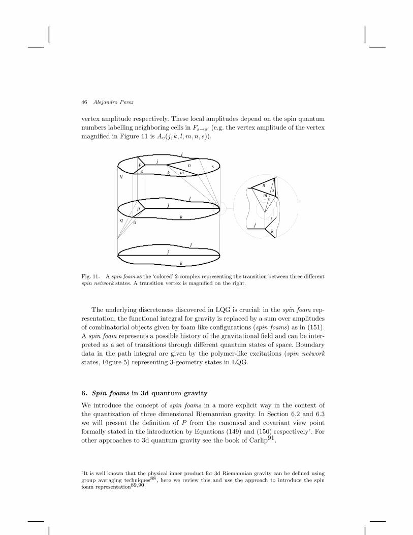
46 Alejandro Perez

vertex amplitude respectively. These local amplitudes depend on the spin quantum

numbers labelling neighboring cells in Fs→s′ (e.g. the vertex amplitude of the vertex

magnified in Figure 11 is Av(j, k, l,m, n, s)).

j

j

j

k

k

k

l

l

l

p

oq

q

po m

n s

jk

l

m

ns

Fig. 11. A spin foam as the ‘colored’ 2-complex representing the transition between three differentspin network states. A transition vertex is magnified on the right.

The underlying discreteness discovered in LQG is crucial: in the spin foam rep-

resentation, the functional integral for gravity is replaced by a sum over amplitudes

of combinatorial objects given by foam-like configurations (spin foams) as in (151).

A spin foam represents a possible history of the gravitational field and can be inter-

preted as a set of transitions through different quantum states of space. Boundary

data in the path integral are given by the polymer-like excitations (spin network

states, Figure 5) representing 3-geometry states in LQG.

6. Spin foams in 3d quantum gravity

We introduce the concept of spin foams in a more explicit way in the context of

the quantization of three dimensional Riemannian gravity. In Section 6.2 and 6.3

we will present the definition of P from the canonical and covariant view point

formally stated in the introduction by Equations (149) and (150) respectivelyr. For

other approaches to 3d quantum gravity see the book of Carlip91.

rIt is well known that the physical inner product for 3d Riemannian gravity can be defined usinggroup averaging techniques88, here we review this and use the approach to introduce the spinfoam representation89,90.

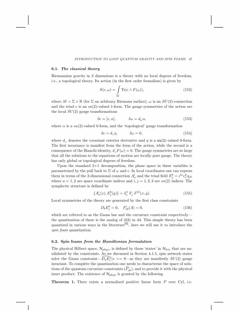
INTRODUCTION TO LOOP QUANTUM GRAVITY AND SPIN FOAMS 47

6.1. The classical theory

Riemannian gravity in 3 dimensions is a theory with no local degrees of freedom,

i.e., a topological theory. Its action (in the first order formalism) is given by

S(e, ω) =

∫

M

Tr(e ∧ F (ω)), (152)

where M = Σ×R (for Σ an arbitrary Riemann surface), ω is an SU(2)-connection

and the triad e is an su(2)-valued 1-form. The gauge symmetries of the action are

the local SU(2) gauge transformations

δe = [e, α] , δω = dωα, (153)

where α is a su(2)-valued 0-form, and the ‘topological’ gauge transformation

δe = dωη, δω = 0, (154)

where dω denotes the covariant exterior derivative and η is a su(2)-valued 0-form.

The first invariance is manifest from the form of the action, while the second is a

consequence of the Bianchi identity, dωF (ω) = 0. The gauge symmetries are so large

that all the solutions to the equations of motion are locally pure gauge. The theory

has only global or topological degrees of freedom.

Upon the standard 2+1 decomposition, the phase space in these variables is

parametrized by the pull back to Σ of ω and e. In local coordinates one can express

them in terms of the 2-dimensional connection Aia and the triad field Eb

j = ǫbcekcηjk

where a = 1, 2 are space coordinate indices and i, j = 1, 2, 3 are su(2) indices. The

symplectic structure is defined by

Aia(x), Eb

j (y) = δ ba δ

ij δ

(2)(x, y). (155)

Local symmetries of the theory are generated by the first class constraints

DbEbj = 0, F i

ab(A) = 0, (156)

which are referred to as the Gauss law and the curvature constraint respectively—

the quantization of these is the analog of (63) in 4d. This simple theory has been

quantized in various ways in the literature91, here we will use it to introduce the

spin foam quantization.

6.2. Spin foams from the Hamiltonian formulation

The physical Hilbert space, Hphys, is defined by those ‘states’ in Hkin that are an-

nihilated by the constraints. As we discussed in Section 4.1.5, spin network states

solve the Gauss constraint—DaEai |s >= 0—as they are manifestly SU(2) gauge

invariant. To complete the quantization one needs to characterize the space of solu-

tions of the quantum curvature constraints (F iab), and to provide it with the physical

inner product. The existence of Hphys is granted by the following

Theorem 1. There exists a normalized positive linear form P over Cyl, i.e.

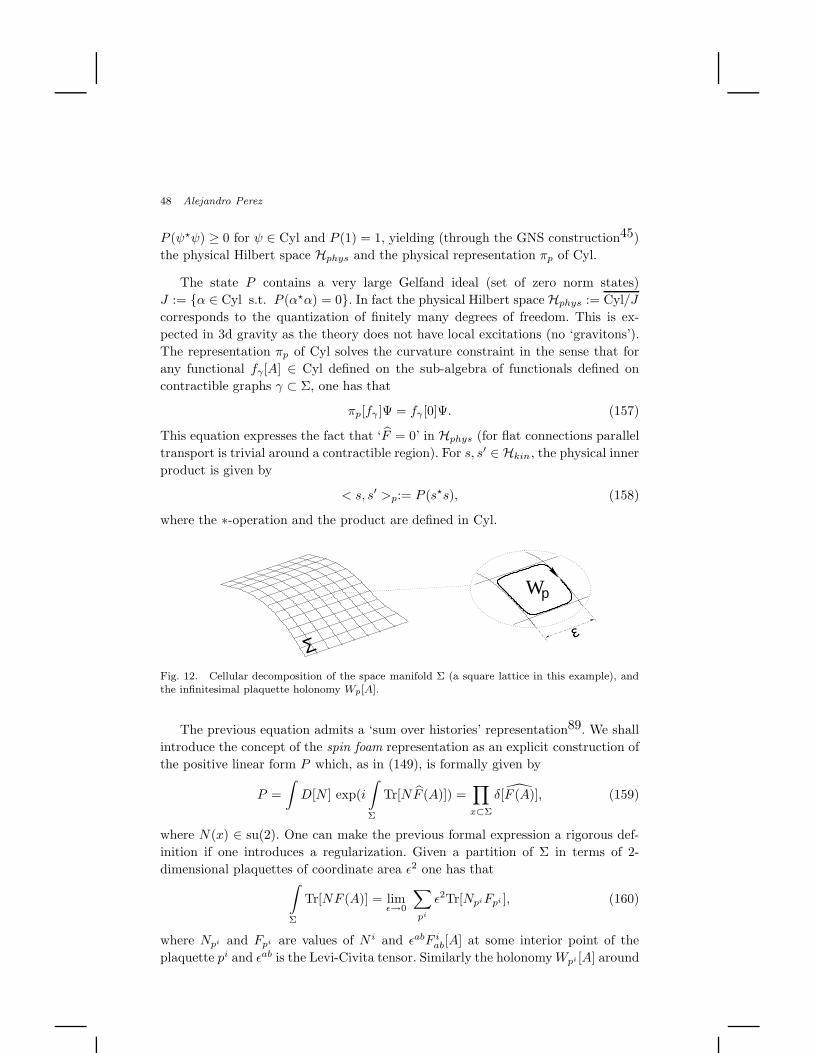
48 Alejandro Perez

P (ψ⋆ψ) ≥ 0 for ψ ∈ Cyl and P (1) = 1, yielding (through the GNS construction45)

the physical Hilbert space Hphys and the physical representation πp of Cyl.

The state P contains a very large Gelfand ideal (set of zero norm states)

J := α ∈ Cyl s.t. P (α⋆α) = 0. In fact the physical Hilbert space Hphys := Cyl/J

corresponds to the quantization of finitely many degrees of freedom. This is ex-

pected in 3d gravity as the theory does not have local excitations (no ‘gravitons’).

The representation πp of Cyl solves the curvature constraint in the sense that for

any functional fγ [A] ∈ Cyl defined on the sub-algebra of functionals defined on

contractible graphs γ ⊂ Σ, one has that

πp[fγ ]Ψ = fγ [0]Ψ. (157)

This equation expresses the fact that ‘F = 0’ in Hphys (for flat connections parallel

transport is trivial around a contractible region). For s, s′ ∈ Hkin, the physical inner

product is given by

< s, s′ >p:= P (s⋆s), (158)

where the ∗-operation and the product are defined in Cyl.

Wp

εΣ

Fig. 12. Cellular decomposition of the space manifold Σ (a square lattice in this example), andthe infinitesimal plaquette holonomy Wp[A].

The previous equation admits a ‘sum over histories’ representation89. We shall

introduce the concept of the spin foam representation as an explicit construction of

the positive linear form P which, as in (149), is formally given by

P =

∫D[N ] exp(i

∫

Σ

Tr[NF (A)]) =∏

x⊂Σ

δ[F (A)], (159)

where N(x) ∈ su(2). One can make the previous formal expression a rigorous def-

inition if one introduces a regularization. Given a partition of Σ in terms of 2-

dimensional plaquettes of coordinate area ǫ2 one has that∫

Σ

Tr[NF (A)] = limǫ→0

∑

pi

ǫ2Tr[NpiFpi ], (160)

where Npi and Fpi are values of N i and ǫabF iab[A] at some interior point of the

plaquette pi and ǫab is the Levi-Civita tensor. Similarly the holonomyWpi [A] around

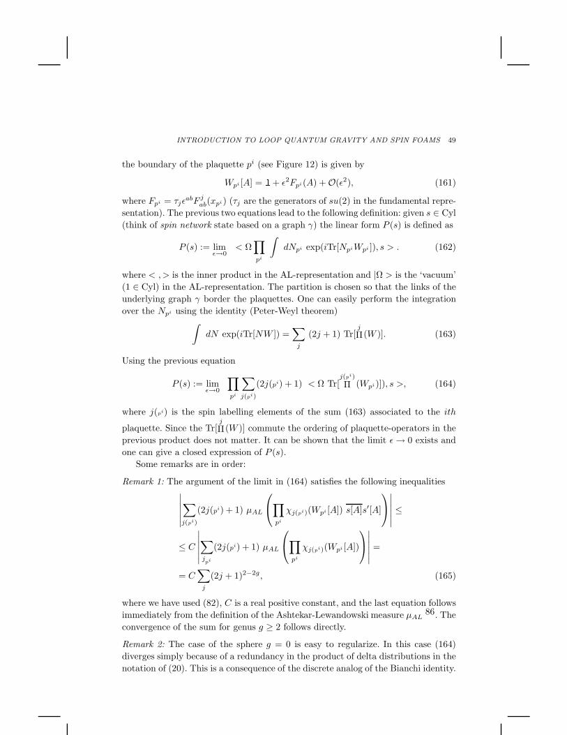
INTRODUCTION TO LOOP QUANTUM GRAVITY AND SPIN FOAMS 49

the boundary of the plaquette pi (see Figure 12) is given by

Wpi [A] = 1+ ǫ2Fpi(A) + O(ǫ2), (161)

where Fpi = τjǫabF j

ab(xpi) (τj are the generators of su(2) in the fundamental repre-

sentation). The previous two equations lead to the following definition: given s ∈ Cyl

(think of spin network state based on a graph γ) the linear form P (s) is defined as

P (s) := limǫ→0

< Ω∏

pi

∫dNpi exp(iTr[NpiWpi ]), s > . (162)

where < ,> is the inner product in the AL-representation and |Ω > is the ‘vacuum’

(1 ∈ Cyl) in the AL-representation. The partition is chosen so that the links of the

underlying graph γ border the plaquettes. One can easily perform the integration

over the Npi using the identity (Peter-Weyl theorem)∫

dN exp(iTr[NW ]) =∑

j

(2j + 1) Tr[j

Π(W )]. (163)

Using the previous equation

P (s) := limǫ→0

∏

pi

∑

j(pi)

(2j(pi) + 1) < Ω Tr[j(pi)

Π (Wpi)]), s >, (164)

where j(pi) is the spin labelling elements of the sum (163) associated to the ith

plaquette. Since the Tr[j

Π(W )] commute the ordering of plaquette-operators in the

previous product does not matter. It can be shown that the limit ǫ→ 0 exists and

one can give a closed expression of P (s).

Some remarks are in order:

Remark 1: The argument of the limit in (164) satisfies the following inequalities∣∣∣∣∣∣

∑

j(pi)

(2j(pi) + 1) µAL

∏

pi

χj(pi)(Wpi [A]) s[A]s′[A]

∣∣∣∣∣∣≤

≤ C

∣∣∣∣∣∣

∑

jpi

(2j(pi) + 1) µAL

∏

pi

χj(pi)(Wpi [A])

∣∣∣∣∣∣=

= C∑

j

(2j + 1)2−2g, (165)

where we have used (82), C is a real positive constant, and the last equation follows

immediately from the definition of the Ashtekar-Lewandowski measure µAL86. The

convergence of the sum for genus g ≥ 2 follows directly.

Remark 2: The case of the sphere g = 0 is easy to regularize. In this case (164)

diverges simply because of a redundancy in the product of delta distributions in the

notation of (20). This is a consequence of the discrete analog of the Bianchi identity.

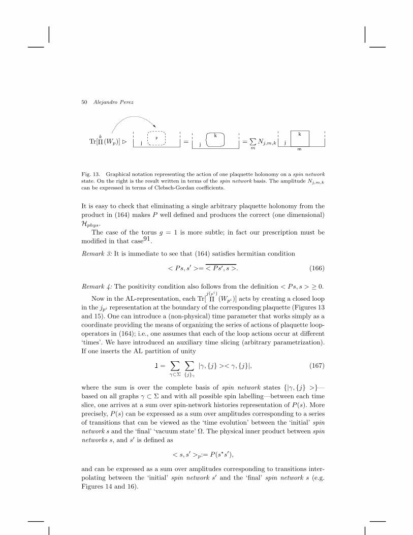
50 Alejandro Perez

Tr[k

Π(Wp)] j

.

P= j

k=

∑mNj,m,k j

m

k

Fig. 13. Graphical notation representing the action of one plaquette holonomy on a spin network

state. On the right is the result written in terms of the spin network basis. The amplitude Nj,m,k

can be expressed in terms of Clebsch-Gordan coefficients.

It is easy to check that eliminating a single arbitrary plaquette holonomy from the

product in (164) makes P well defined and produces the correct (one dimensional)

Hphys.

The case of the torus g = 1 is more subtle; in fact our prescription must be

modified in that case91.

Remark 3: It is immediate to see that (164) satisfies hermitian condition

< Ps, s′ >= < Ps′, s >. (166)

Remark 4: The positivity condition also follows from the definition < Ps, s > ≥ 0.

Now in the AL-representation, each Tr[j(pi)

Π (Wpi )] acts by creating a closed loop

in the jpi representation at the boundary of the corresponding plaquette (Figures 13

and 15). One can introduce a (non-physical) time parameter that works simply as a

coordinate providing the means of organizing the series of actions of plaquette loop-

operators in (164); i.e., one assumes that each of the loop actions occur at different

‘times’. We have introduced an auxiliary time slicing (arbitrary parametrization).

If one inserts the AL partition of unity1 =∑

γ⊂Σ

∑

jγ

|γ, j >< γ, j|, (167)

where the sum is over the complete basis of spin network states |γ, j >—based on all graphs γ ⊂ Σ and with all possible spin labelling—between each time

slice, one arrives at a sum over spin-network histories representation of P (s). More

precisely, P (s) can be expressed as a sum over amplitudes corresponding to a series

of transitions that can be viewed as the ‘time evolution’ between the ‘initial’ spin

network s and the ‘final’ ‘vacuum state’ Ω. The physical inner product between spin

networks s, and s′ is defined as

< s, s′ >p:= P (s⋆s′),

and can be expressed as a sum over amplitudes corresponding to transitions inter-

polating between the ‘initial’ spin network s′ and the ‘final’ spin network s (e.g.

Figures 14 and 16).

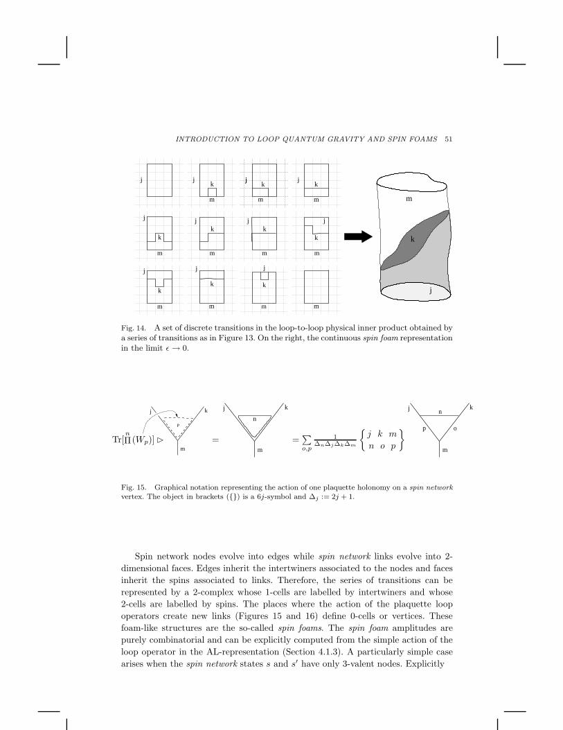
INTRODUCTION TO LOOP QUANTUM GRAVITY AND SPIN FOAMS 51

j

m

k

j

m

k

j

jk

m

m

jk

m

j

k

jjk

m

m

jk

m

k

j

j

m

k

m

k

j

m

k

m

j

Fig. 14. A set of discrete transitions in the loop-to-loop physical inner product obtained bya series of transitions as in Figure 13. On the right, the continuous spin foam representationin the limit ǫ→ 0.

Tr[n

Π(Wp)]

.

j k

m

P

=

.

j k

m

n

=∑o,p

1∆n∆j∆k∆m

j k m

n o p

.

j k

m

p o

n

Fig. 15. Graphical notation representing the action of one plaquette holonomy on a spin network

vertex. The object in brackets () is a 6j-symbol and ∆j := 2j + 1.

Spin network nodes evolve into edges while spin network links evolve into 2-

dimensional faces. Edges inherit the intertwiners associated to the nodes and faces

inherit the spins associated to links. Therefore, the series of transitions can be

represented by a 2-complex whose 1-cells are labelled by intertwiners and whose

2-cells are labelled by spins. The places where the action of the plaquette loop

operators create new links (Figures 15 and 16) define 0-cells or vertices. These

foam-like structures are the so-called spin foams. The spin foam amplitudes are

purely combinatorial and can be explicitly computed from the simple action of the

loop operator in the AL-representation (Section 4.1.3). A particularly simple case

arises when the spin network states s and s′ have only 3-valent nodes. Explicitly

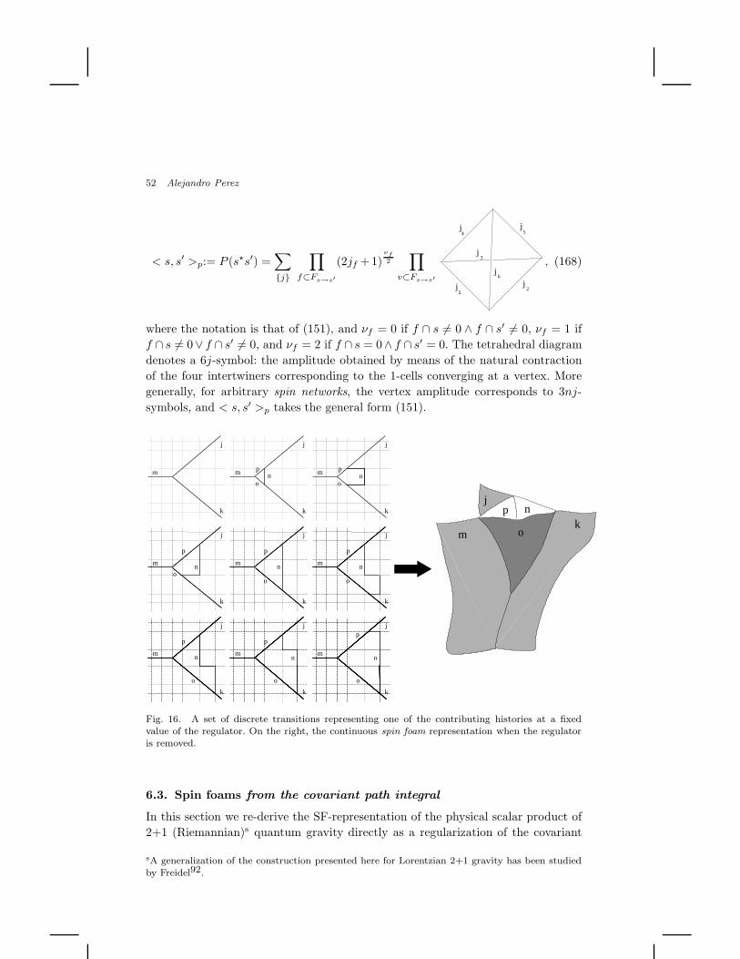
52 Alejandro Perez

< s, s′ >p:= P (s⋆s′) =∑

j

∏

f⊂Fs→s′

(2jf +1)νf2

∏

v⊂Fs→s′

j

j

j

j

j1

2

3

4 5

6j

, (168)

where the notation is that of (151), and νf = 0 if f ∩ s 6= 0 ∧ f ∩ s′ 6= 0, νf = 1 if

f ∩ s 6= 0∨ f ∩ s′ 6= 0, and νf = 2 if f ∩ s = 0∧ f ∩ s′ = 0. The tetrahedral diagram

denotes a 6j-symbol: the amplitude obtained by means of the natural contraction

of the four intertwiners corresponding to the 1-cells converging at a vertex. More

generally, for arbitrary spin networks, the vertex amplitude corresponds to 3nj-

symbols, and < s, s′ >p takes the general form (151).

m

j

k

m

on

k

j

p

m n

k

j

p

o

m

j

k

o

pn

m n

k

j

p

o

m

k

j

p

o

n

m p

on

k

j

m n

k

j

p

o

m

k

j

o

n

p

j

mk

o

p n

Fig. 16. A set of discrete transitions representing one of the contributing histories at a fixedvalue of the regulator. On the right, the continuous spin foam representation when the regulatoris removed.

6.3. Spin foams from the covariant path integral

In this section we re-derive the SF-representation of the physical scalar product of

2+1 (Riemannian)s quantum gravity directly as a regularization of the covariant

sA generalization of the construction presented here for Lorentzian 2+1 gravity has been studiedby Freidel92.

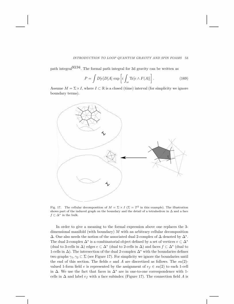
INTRODUCTION TO LOOP QUANTUM GRAVITY AND SPIN FOAMS 53

path integral93,94. The formal path integral for 3d gravity can be written as

P =

∫D[e]D[A] exp

[i

∫

M

Tr[e ∧ F (A)]

]. (169)

Assume M = Σ×I, where I ⊂ R is a closed (time) interval (for simplicity we ignore

boundary terms).

f

Σ

Σ

Fig. 17. The cellular decomposition of M = Σ × I (Σ = T 2 in this example). The illustrationshows part of the induced graph on the boundary and the detail of a tetrahedron in ∆ and a facef ⊂ ∆⋆ in the bulk.

In order to give a meaning to the formal expression above one replaces the 3-

dimensional manifold (with boundary) M with an arbitrary cellular decomposition

∆. One also needs the notion of the associated dual 2-complex of ∆ denoted by ∆⋆.

The dual 2-complex ∆⋆ is a combinatorial object defined by a set of vertices v ⊂ ∆⋆

(dual to 3-cells in ∆) edges e ⊂ ∆⋆ (dual to 2-cells in ∆) and faces f ⊂ ∆⋆ (dual to

1-cells in ∆). The intersection of the dual 2-complex ∆⋆ with the boundaries defines

two graphs γ1, γ2 ⊂ Σ (see Figure 17). For simplicity we ignore the boundaries until

the end of this section. The fields e and A are discretized as follows. The su(2)-

valued 1-form field e is represented by the assignment of ef ∈ su(2) to each 1-cell

in ∆. We use the fact that faces in ∆⋆ are in one-to-one correspondence with 1-

cells in ∆ and label ef with a face subindex (Figure 17). The connection field A is

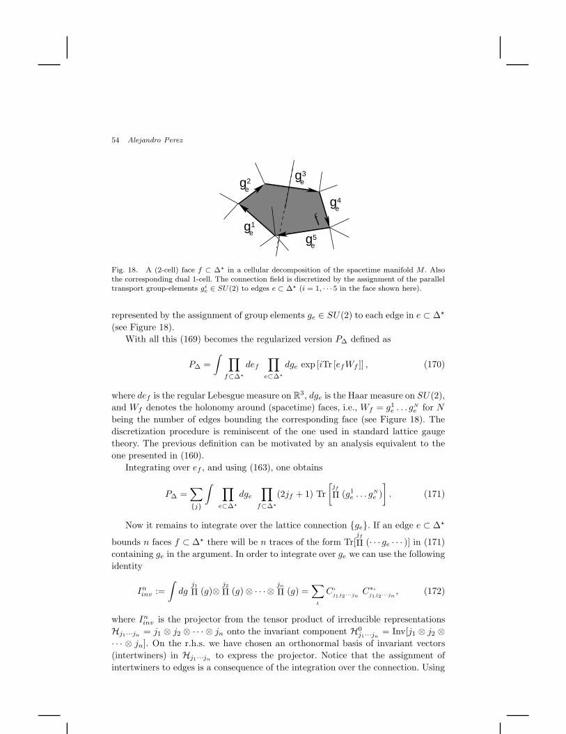
54 Alejandro Perez

f

ge

g3e

g4e

g5e

g1e

2

Fig. 18. A (2-cell) face f ⊂ ∆⋆ in a cellular decomposition of the spacetime manifold M . Alsothe corresponding dual 1-cell. The connection field is discretized by the assignment of the paralleltransport group-elements gi

e ∈ SU(2) to edges e ⊂ ∆⋆ (i = 1, · · · 5 in the face shown here).

represented by the assignment of group elements ge ∈ SU(2) to each edge in e ⊂ ∆⋆

(see Figure 18).

With all this (169) becomes the regularized version P∆ defined as

P∆ =

∫ ∏

f⊂∆⋆

def

∏

e⊂∆⋆

dge exp [iTr [efWf ]] , (170)

where def is the regular Lebesgue measure on R3, dge is the Haar measure on SU(2),

and Wf denotes the holonomy around (spacetime) faces, i.e., Wf = g1e . . . g

Ne for N

being the number of edges bounding the corresponding face (see Figure 18). The

discretization procedure is reminiscent of the one used in standard lattice gauge

theory. The previous definition can be motivated by an analysis equivalent to the

one presented in (160).

Integrating over ef , and using (163), one obtains

P∆ =∑

j

∫ ∏

e⊂∆⋆

dge

∏

f⊂∆⋆

(2jf + 1) Tr

[jf

Π (g1e . . . g

N

e )

]. (171)

Now it remains to integrate over the lattice connection ge. If an edge e ⊂ ∆⋆

bounds n faces f ⊂ ∆⋆ there will be n traces of the form Tr[jf

Π (· · · ge · · · )] in (171)

containing ge in the argument. In order to integrate over ge we can use the following

identity

Ininv :=

∫dg

j1Π (g)⊗

j2Π (g) ⊗ · · · ⊗

jn

Π (g) =∑

ι

Cι

j1j2···jnC∗ι

j1j2···jn, (172)

where Ininv is the projector from the tensor product of irreducible representations

Hj1···jn = j1 ⊗ j2 ⊗ · · · ⊗ jn onto the invariant component H0j1···jn

= Inv[j1 ⊗ j2 ⊗· · · ⊗ jn]. On the r.h.s. we have chosen an orthonormal basis of invariant vectors

(intertwiners) in Hj1···jn to express the projector. Notice that the assignment of

intertwiners to edges is a consequence of the integration over the connection. Using

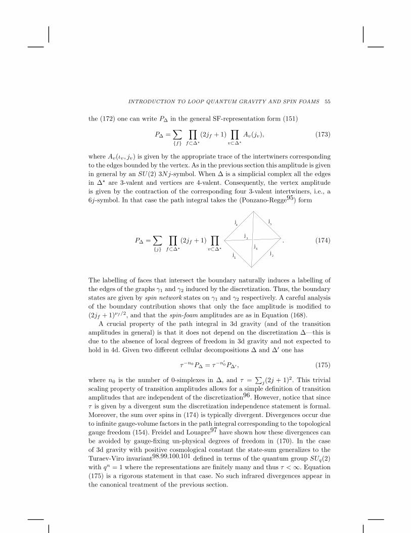
INTRODUCTION TO LOOP QUANTUM GRAVITY AND SPIN FOAMS 55

the (172) one can write P∆ in the general SF-representation form (151)

P∆ =∑

f

∏

f⊂∆⋆

(2jf + 1)∏

v⊂∆⋆

Av(jv), (173)

where Av(ιv, jv) is given by the appropriate trace of the intertwiners corresponding

to the edges bounded by the vertex. As in the previous section this amplitude is given

in general by an SU(2) 3Nj-symbol. When ∆ is a simplicial complex all the edges

in ∆⋆ are 3-valent and vertices are 4-valent. Consequently, the vertex amplitude

is given by the contraction of the corresponding four 3-valent intertwiners, i.e., a

6j-symbol. In that case the path integral takes the (Ponzano-Regge95) form

P∆ =∑

j

∏

f⊂∆⋆

(2jf + 1)∏

v⊂∆⋆

j

j

j

j

j1

2

3

4 5

6j

. (174)

The labelling of faces that intersect the boundary naturally induces a labelling of

the edges of the graphs γ1 and γ2 induced by the discretization. Thus, the boundary

states are given by spin network states on γ1 and γ2 respectively. A careful analysis

of the boundary contribution shows that only the face amplitude is modified to

(2jf + 1)νf /2, and that the spin-foam amplitudes are as in Equation (168).

A crucial property of the path integral in 3d gravity (and of the transition

amplitudes in general) is that it does not depend on the discretization ∆—this is

due to the absence of local degrees of freedom in 3d gravity and not expected to

hold in 4d. Given two different cellular decompositions ∆ and ∆′ one has

τ−n0P∆ = τ−n′0P∆′ , (175)

where n0 is the number of 0-simplexes in ∆, and τ =∑

j(2j + 1)2. This trivial

scaling property of transition amplitudes allows for a simple definition of transition

amplitudes that are independent of the discretization96. However, notice that since

τ is given by a divergent sum the discretization independence statement is formal.

Moreover, the sum over spins in (174) is typically divergent. Divergences occur due

to infinite gauge-volume factors in the path integral corresponding to the topological

gauge freedom (154). Freidel and Louapre97 have shown how these divergences can

be avoided by gauge-fixing un-physical degrees of freedom in (170). In the case

of 3d gravity with positive cosmological constant the state-sum generalizes to the

Turaev-Viro invariant98,99,100,101 defined in terms of the quantum group SUq(2)

with qn = 1 where the representations are finitely many and thus τ <∞. Equation

(175) is a rigorous statement in that case. No such infrared divergences appear in

the canonical treatment of the previous section.

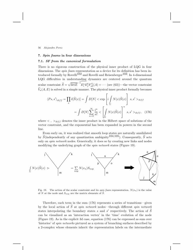
56 Alejandro Perez

7. Spin foams in four dimensions

7.1. SF from the canonical formulation

There is no rigorous construction of the physical inner product of LQG in four

dimensions. The spin foam representation as a device for its definition has been in-

troduced formally by Rovelli102 and Rovelli and Reisenberger103. In 4-dimensional

LQG difficulties in understanding dynamics are centered around the quantum

scalar constraint S =√

detE−1Ea

i EbjF

ijab(A) + · · · (see (63))—the vector constraint

Va(A,E) is solved in a simple manner. The physical inner product formally becomes

〈Ps, s′〉diff =∏

x

δ[S(x)] =

∫D[N ] < exp

i∫

Σ

N(x)S(x)

s, s′ >diff

=

∫D[N ]

∞∑

n=0

in

n!<

∫

Σ

N(x)S(x)

n

s, s′ >diff , (176)

where < , >diff denotes the inner product in the Hilbert space of solutions of the

vector constraint, and the exponential has been expanded in powers in the second

line.

From early on, it was realized that smooth loop states are naturally annihilated

by S(independently of any quantization ambiguity104,105). Consequently, S acts

only on spin network nodes. Generically, it does so by creating new links and nodes

modifying the underlying graph of the spin network states (Figure 19).

∫Σ

N(x)S(x)

.

j k

m

=∑nop

N(xn)Snop

.

j k

m

p o

n

j

p

on

k

m

Fig. 19. The action of the scalar constraint and its spin foam representation. N(xn) is the valueof N at the node and Snop are the matrix elements of S.

Therefore, each term in the sum (176) represents a series of transitions—given

by the local action of S at spin network nodes—through different spin network

states interpolating the boundary states s and s′ respectively. The action of S

can be visualized as an ‘interaction vertex’ in the ‘time’ evolution of the node

(Figure 19). As in the explicit 3d case, equation (176) can be expressed as sum over

‘histories’ of spin networks pictured as a system of branching surfaces described by

a 2-complex whose elements inherit the representation labels on the intermediate

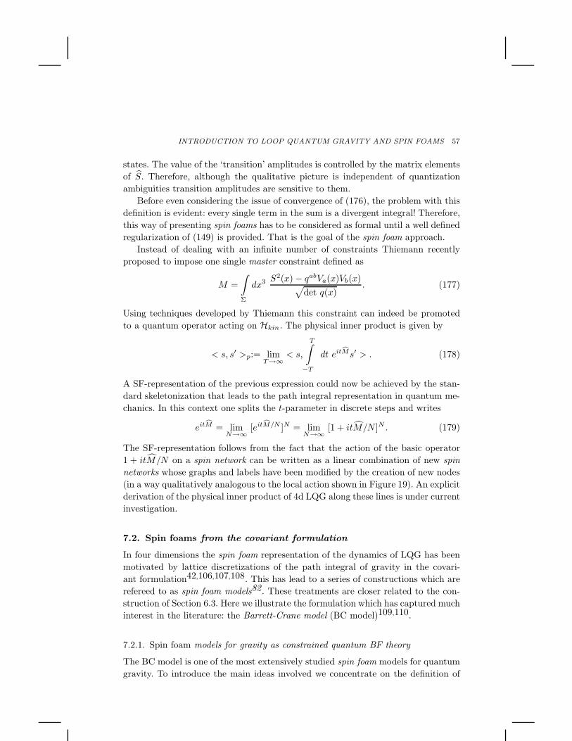
INTRODUCTION TO LOOP QUANTUM GRAVITY AND SPIN FOAMS 57

states. The value of the ‘transition’ amplitudes is controlled by the matrix elements

of S. Therefore, although the qualitative picture is independent of quantization

ambiguities transition amplitudes are sensitive to them.

Before even considering the issue of convergence of (176), the problem with this

definition is evident: every single term in the sum is a divergent integral! Therefore,

this way of presenting spin foams has to be considered as formal until a well defined

regularization of (149) is provided. That is the goal of the spin foam approach.

Instead of dealing with an infinite number of constraints Thiemann recently

proposed to impose one single master constraint defined as

M =

∫

Σ

dx3 S2(x) − qabVa(x)Vb(x)√det q(x)

. (177)

Using techniques developed by Thiemann this constraint can indeed be promoted

to a quantum operator acting on Hkin. The physical inner product is given by

< s, s′ >p:= limT→∞

< s,

T∫

−T

dt eitMs′ > . (178)

A SF-representation of the previous expression could now be achieved by the stan-

dard skeletonization that leads to the path integral representation in quantum me-

chanics. In this context one splits the t-parameter in discrete steps and writes

eitM = limN→∞

[eitM/N ]N = limN→∞

[1 + itM/N ]N . (179)

The SF-representation follows from the fact that the action of the basic operator

1 + itM/N on a spin network can be written as a linear combination of new spin

networks whose graphs and labels have been modified by the creation of new nodes

(in a way qualitatively analogous to the local action shown in Figure 19). An explicit

derivation of the physical inner product of 4d LQG along these lines is under current

investigation.

7.2. Spin foams from the covariant formulation

In four dimensions the spin foam representation of the dynamics of LQG has been

motivated by lattice discretizations of the path integral of gravity in the covari-

ant formulation42,106,107,108. This has lead to a series of constructions which are

refereed to as spin foam models82. These treatments are closer related to the con-

struction of Section 6.3. Here we illustrate the formulation which has captured much

interest in the literature: the Barrett-Crane model (BC model)109,110.

7.2.1. Spin foam models for gravity as constrained quantum BF theory

The BC model is one of the most extensively studied spin foam models for quantum

gravity. To introduce the main ideas involved we concentrate on the definition of

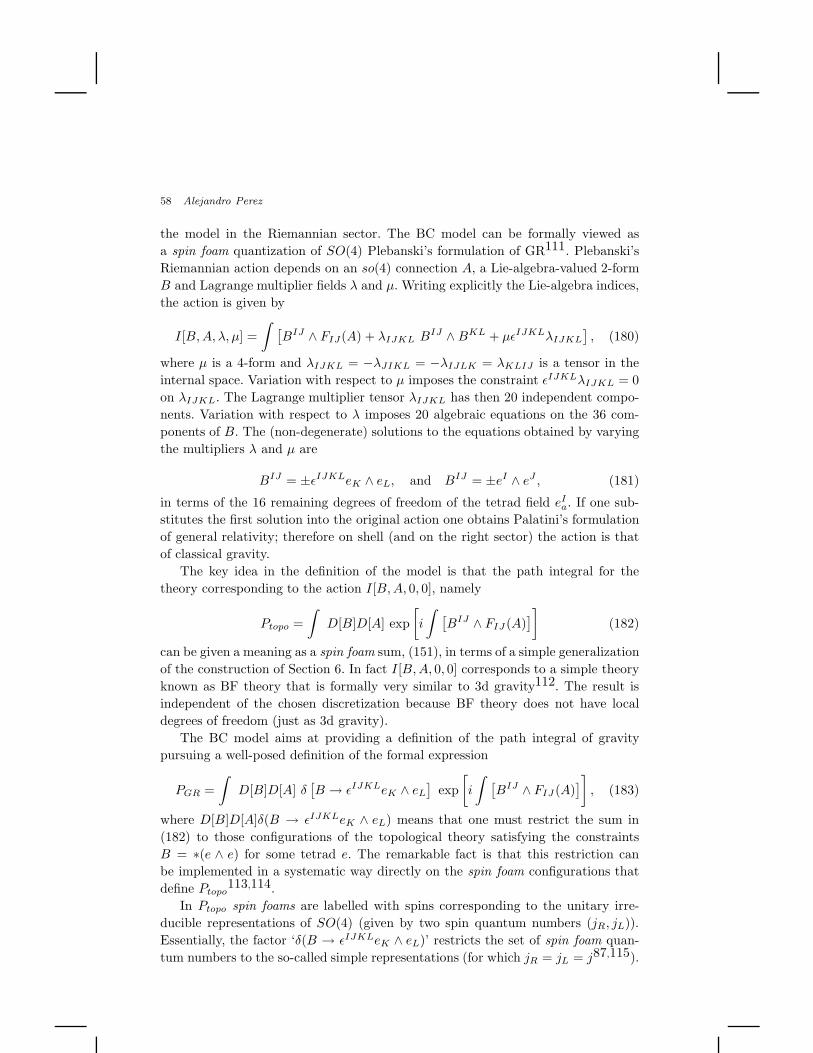
58 Alejandro Perez

the model in the Riemannian sector. The BC model can be formally viewed as

a spin foam quantization of SO(4) Plebanski’s formulation of GR111. Plebanski’s

Riemannian action depends on an so(4) connection A, a Lie-algebra-valued 2-form

B and Lagrange multiplier fields λ and µ. Writing explicitly the Lie-algebra indices,

the action is given by

I[B,A, λ, µ] =

∫ [BIJ ∧ FIJ(A) + λIJKL BIJ ∧BKL + µǫIJKLλIJKL

], (180)

where µ is a 4-form and λIJKL = −λJIKL = −λIJLK = λKLIJ is a tensor in the

internal space. Variation with respect to µ imposes the constraint ǫIJKLλIJKL = 0

on λIJKL. The Lagrange multiplier tensor λIJKL has then 20 independent compo-

nents. Variation with respect to λ imposes 20 algebraic equations on the 36 com-

ponents of B. The (non-degenerate) solutions to the equations obtained by varying

the multipliers λ and µ are

BIJ = ±ǫIJKLeK ∧ eL, and BIJ = ±eI ∧ eJ , (181)

in terms of the 16 remaining degrees of freedom of the tetrad field eIa. If one sub-

stitutes the first solution into the original action one obtains Palatini’s formulation

of general relativity; therefore on shell (and on the right sector) the action is that

of classical gravity.

The key idea in the definition of the model is that the path integral for the

theory corresponding to the action I[B,A, 0, 0], namely

Ptopo =

∫D[B]D[A] exp

[i

∫ [BIJ ∧ FIJ (A)

]](182)

can be given a meaning as a spin foam sum, (151), in terms of a simple generalization

of the construction of Section 6. In fact I[B,A, 0, 0] corresponds to a simple theory

known as BF theory that is formally very similar to 3d gravity112. The result is

independent of the chosen discretization because BF theory does not have local

degrees of freedom (just as 3d gravity).

The BC model aims at providing a definition of the path integral of gravity

pursuing a well-posed definition of the formal expression

PGR =

∫D[B]D[A] δ

[B → ǫIJKLeK ∧ eL

]exp

[i

∫ [BIJ ∧ FIJ (A)

]], (183)

where D[B]D[A]δ(B → ǫIJKLeK ∧ eL) means that one must restrict the sum in

(182) to those configurations of the topological theory satisfying the constraints

B = ∗(e ∧ e) for some tetrad e. The remarkable fact is that this restriction can

be implemented in a systematic way directly on the spin foam configurations that

define Ptopo113,114.

In Ptopo spin foams are labelled with spins corresponding to the unitary irre-

ducible representations of SO(4) (given by two spin quantum numbers (jR, jL)).

Essentially, the factor ‘δ(B → ǫIJKLeK ∧ eL)’ restricts the set of spin foam quan-

tum numbers to the so-called simple representations (for which jR = jL = j87,115).

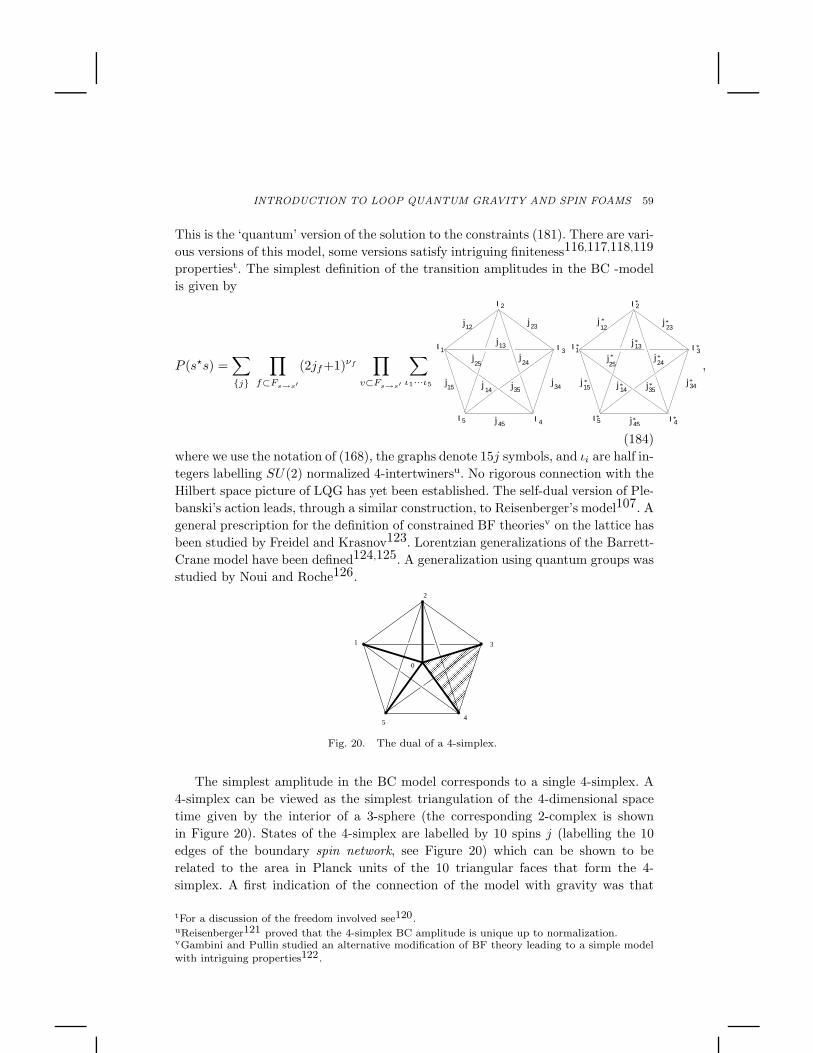
INTRODUCTION TO LOOP QUANTUM GRAVITY AND SPIN FOAMS 59

This is the ‘quantum’ version of the solution to the constraints (181). There are vari-

ous versions of this model, some versions satisfy intriguing finiteness116,117,118,119

propertiest. The simplest definition of the transition amplitudes in the BC -model

is given by

P (s⋆s) =∑

j

∏

f⊂Fs→s′

(2jf+1)νf

∏

v⊂Fs→s′

∑

ι1···ι5

2

ι 1

ι 5 j45ι 4

j

3ι

j

ι

j24

j j35

2

13ι 1

ι 5 j45ι 4

34j

3ι

j

ι

j

j

24

j14 j35j

*

*

*

*

*

*

*

**

*

*

*

*

j12 23

j25

j13

1415j 34

j*25

15

j12*

23

,

(184)

where we use the notation of (168), the graphs denote 15j symbols, and ιi are half in-

tegers labelling SU(2) normalized 4-intertwinersu. No rigorous connection with the

Hilbert space picture of LQG has yet been established. The self-dual version of Ple-

banski’s action leads, through a similar construction, to Reisenberger’s model107. A

general prescription for the definition of constrained BF theoriesv on the lattice has

been studied by Freidel and Krasnov123. Lorentzian generalizations of the Barrett-

Crane model have been defined124,125. A generalization using quantum groups was

studied by Noui and Roche126.

1

2

3

45

0

Fig. 20. The dual of a 4-simplex.

The simplest amplitude in the BC model corresponds to a single 4-simplex. A

4-simplex can be viewed as the simplest triangulation of the 4-dimensional space

time given by the interior of a 3-sphere (the corresponding 2-complex is shown

in Figure 20). States of the 4-simplex are labelled by 10 spins j (labelling the 10

edges of the boundary spin network, see Figure 20) which can be shown to be

related to the area in Planck units of the 10 triangular faces that form the 4-

simplex. A first indication of the connection of the model with gravity was that

tFor a discussion of the freedom involved see120.uReisenberger121 proved that the 4-simplex BC amplitude is unique up to normalization.vGambini and Pullin studied an alternative modification of BF theory leading to a simple modelwith intriguing properties122.

60 Alejandro Perez

the large j-asymptotics appeared to be dominated by the exponential of the Regge

action127,128 (the action derived by Regge as a discretization of GR). This estimate

was done using the stationary phase approximation to the integral129 that gives

the amplitude of a 4-simplex in the BC model. However, more detailed calculations

showed that the amplitude is dominated by configurations corresponding to degen-

erate 4-simplexes130,97,131. This seem to invalidate a simple connection to GR and

is one of the main puzzles in the model.

7.3. Spin foams as Feynman diagrams

The main problem with the models of the previous section is that they are defined

on a discretization ∆ of M and that—contrary to what happens with a topological

theory, e.g. 3d gravity (Equation 175)—the amplitudes depend on the discretiza-

tion ∆. Various possibilities to eliminate this regulator have been discussed in the

literature but no explicit results are yet known in 4d. An interesting proposal is a

discretization-independent definition of spin foam models achieved by the introduc-

tion of an auxiliary field theory living on an abstract group manifold—Spin(4)4 and

SL(2, C)4 for Riemannian and Lorentzian gravity respectively132,133,134,135,136.

The action of the auxiliary group field theory (GFT) takes the form

I[φ] =

∫

G4

φ2 +λ

5!

∫

G10

M (5)[φ], (185)

where M (5)[φ] is a fifth order monomial, and G is the corresponding group. In the

simplest model M (5)[φ] =

φ(g1, g2, g3, g4)φ(g4, g5, g6, g7)φ(g7, g3, g8, g9)φ(g9, g6, g2, g10)φ(g10, g8, g5, g1).

The field φ is required to be invariant under the (simultaneous) right action of

the group on its four arguments in addition to other symmetries (not described

here for simplicity). The perturbative expansion in λ of the GFT Euclidean path

integral is given by

P =

∫D[φ]e−I[φ] =

∑

FN

λN

sym[FN ]A[FN ], (186)

where A[FN ] corresponds to a sum of Feynman-diagram amplitudes for diagrams

with N interaction vertices, and sym[FN ] denotes the standard symmetry factor. A

remarkable property of this expansion is that A[FN ] can be expressed as a sum over

spin foam amplitudes, i.e., 2-complexes labelled by unitary irreducible representa-

tions of G. Moreover, for very simple interaction M (5)[φ], the spin foam amplitudes

are in one-to-one correspondence to those found in the models of the previous section

(e.g. the BC model). This duality is regarded as a way of providing a fully com-

binatorial definition of quantum gravity where no reference to any discretization

or even a manifold-structure is made. Transition amplitudes between spin network

states correspond to n-point functions of the field theory137. These models have

been inspired by generalizations of matrix models applied to BF theory138,139.

INTRODUCTION TO LOOP QUANTUM GRAVITY AND SPIN FOAMS 61

Divergent transition amplitudes can arise by the contribution of ‘loop’ diagrams

as in standard QFT. In spin foams, diagrams corresponding to 2-dimensional bub-

bles are potentially divergent because spin labels can be arbitrarily high leading to

unbounded sums in (151). Such divergences do not occur in certain field theories

dual (in the sense above) to the Barrett-Crane (BC) model. However, little is known

about the convergence of the series in λ and the physical meaning of this constant.

Nevertheless, Freidel and Louapre140 have shown that the series can be re-summed

in certain models dual to lower dimensional theories. Techniques for studying the

continuum limit of these kind of theories have been proposed141,142,143,144. There

are models defined in this context admitting matter degree of freedom145,146.

7.4. Causal spin foams

Let us finish by presenting a fundamentally different construction leading to spin

foams. Using the kinematical setting of LQG with the assumption of the existence

of a micro-local (in the sense of Planck scale) causal structure Markopoulou and

Smolin147,148,149 define a general class of (causal) spin foam models for gravity.

The elementary transition amplitude AsI→sI+1 from an initial spin network sI to

another spin network sI+1 is defined by a set of simple combinatorial rules based

on a definition of causal propagation of the information at nodes. The rules and

amplitudes have to satisfy certain causal restrictions (motivated by the standard

concepts in classical Lorentzian physics). These rules generate surface-like excita-

tions of the same kind one encounters in the previous formulations. Spin foams

FNsi→sf

are labelled by the number of times, N , these elementary transitions take

place. Transition amplitudes are defined as

〈si, sf 〉 =∑

N

A(FNsi→sf

) (187)

which is of the generic form (151). The models are not related to any continuum

action. The only guiding principles in the construction are the restrictions imposed

by causality, and the requirement of the existence of a non-trivial critical behavior

that reproduces general relativity at large scales. Some indirect evidence of a possible

non trivial continuum limit has been obtained in certain versions of these models

in 1 + 1 dimensions.

8. Some final bibliographic remarks

We did not have time to discuss the applications of loop quantum gravity to cos-

mology. The interested reader is referred to review article150 and the references

therein.

We did not have the chance to mention in this lectures the important area of

research in LQG devoted to the study of the low energy limit of the theory. We

refer the reader to the general sources19,4,20 for bibliography and an overview of

results and outlook.

62 Alejandro Perez

In Section 4 we introduced a representation of the basic kinematical observables

in the kinematical Hilbert space Hkin. That was the starting point for the definition

of the theory. The reader might wonder why one emphasizes so much the Hilbert

space as a fundamental object when in the context of standard quantum field theory

it is rather the algebra of observables what plays the fundamental role. Hilbert

spaces correspond to representations of the algebra of observables which are chosen

according to the physical situation at hand. However, when extra symmetry is

present it can happen that there is no freedom and that a single representation

is selected by the additional symmetry. This is in fact the case in LQG if one

imposes the condition of diffeomorphism invariance on the state that defines the

representation of the holonomy and the flux operators 151,152,153,154,155,156,157.

Acknowledgments

I would like to thank the organizer of the Second International Conference on Fun-

damental Interactions for their support and for a wonderful conference. Special

thanks to them also for their great hospitality and the wonderful time we had in

Pedra Azul. I thank Abhay Ashtekar, Bernd Bruegmann, Rodolfo Gambini, Jurek

Lewandowski, Marcelo Maneschy, Karim Noui and Carlo Rovelli for discussions and

to Mikhail Kagan and Kevin Vandersloot for the careful reading of the manuscript. I

thank Hoi Lai Yu for listening to an early version to these lectures and for insightful

questions. Many thanks to Olivier Piguet and Clisthenis Constantinidis. This work

has been supported by NSF grants PHY-0354932 and INT-0307569 and the Eberly

Research Funds of Penn State University.

References

1. Rogerio Rosenfeld. The standard model. Proceedings of the II International confer-ence on fundamental interactions, Pedra Azul, Brazil, June 2004.

2. R. M. Wald. Quantum field theory in curved space-time and black hole thermody-namics. Chicago, USA: Univ. Pr. (1994) 205 p.

3. R. M. Wald. General relativity. Chicago, Usa: Univ. Pr. ( 1984) 491p.4. C. Rovelli. Quantum Gravity. Cambridge, UK: Univ. Pr. (2004) 480 p.5. Carlo Rovelli. Relational quantum mechanics. quant-ph/9609002, 1995.6. Norbert Grot, Carlo Rovelli, and Ranjeet S. Tate. Time-of-arrival in quantum me-

chanics. Phys. Rev., A54:4679, 1996.7. Rodolfo Gambini and Rafael A. Porto. Relational time in generally covariant quan-

tum systems: Four models. Phys. Rev., D63:105014, 2001.8. Rodolfo Gambini and Rafael A. Porto. Relational reality in relativistic quantum

mechanics. Phys. Lett., A294:129–133, 2002.9. Rodolfo Gambini and Rafael A. Porto. Multi-local relational description of the mea-

surement process in quantum field theory. New J. Phys., 4:58, 2002.10. Rodolfo Gambini and Rafael A. Porto. A physical distinction between a covariant

and non covariant description of the measurement process in relativistic quantumtheories. New. J. Phys., 5:105, 2003.

11. R. Penrose. Gravity and quantum mechanics. Prepared for 13th Conference on Gen-eral Relativity and Gravitation (GR-13), Cordoba, Argentina, 29 Jun - 4 Jul 1992.

INTRODUCTION TO LOOP QUANTUM GRAVITY AND SPIN FOAMS 63

12. R. Penrose. Twistor theory, the einstein equations, and quantum mechanics. Pre-pared for International School of Cosmology and Gravitation: 14th Course: QuantumGravity, Erice, Italy, 11-19 May 1995.

13. R. Penrose. Gravitational collapse of the wavefunction: An experimentally testableproposal. Prepared for 9th Marcel Grossmann Meeting on Recent Developments inTheoretical and Experimental General Relativity, Gravitation and Relativistic FieldTheories (MG 9), Rome, Italy, 2-9 Jul 2000.

14. R. Penrose. The role of gravity in quantum state reduction. Prepared for InternationalConference on Non-Accelerator Particle Physics - ICNAPP, Bangalore, India, 2-9 Jan1994.

15. S. Weinberg. The Quantum Theory of Fields. Cambridge University Press, 1995.16. Robert C. Myers and Maxim Pospelov. Experimental challenges for quantum gravity.

Phys. Rev. Lett., 90:211601, 2003.17. Alejandro Perez and Daniel Sudarsky. Comments on challenges for quantum gravity.

Phys. Rev. Lett., 91:179101, 2003.18. John Collins, Alejandro Perez, Daniel Sudarsky, Luis Urrutia, and Hector Vucetich.

Lorentz invariance: An additional fine-tuning problem. Phys. Rev. Lett. (in press,preprint gr-qc/0403053), 2004.

19. Abhay Ashtekar and Jerzy Lewandowski. Background independent quantum gravity:A status report. Class. Quant. Grav., 21:R53, 2004.

20. Thomas Thiemann. Introduction to modern canonical quantum general relativity.gr-qc/0110034, 2001.

21. L. Smolin. Recent Developments in non Perturbative Quantum Gravity; in QuantumGravity and Cosmology, Proceedings of the 1991 GIFT International Seminar onTheoretical Physics. Available at hep-th/9202022. World Scientific, Singapore, 1992.

22. C. Rovelli and L. Smolin. Discretneess of the area and volume in quantum gravity.Nucl Phys B, 442 (1995), Erratum: 456:593,734, 1995.

23. Ted Jacobson. New variables for canonical supergravity. Class. Quant. Grav., 5:923,1988.

24. H. J. Matschull and H. Nicolai. Canonical quantum supergravity in three-dimensions.Nucl. Phys., B411:609–646, 1994.

25. Yi Ling. Introduction to supersymmetric spin networks. J. Math. Phys., 43:154–169,2002.

26. Yi Ling. Extending loop quantum gravity to supergravity. UMI-30-51694.27. Yi Ling and Lee Smolin. Holographic formulation of quantum supergravity. Phys.

Rev., D63:064010, 2001.28. Etera R. Livine and Robert Oeckl. Three-dimensional quantum supergravity and

supersymmetric spin foam models. Adv. Theor. Math. Phys., 7:951–1001, 2004.29. M. Henneaux and C. Teitelboim. Quantization of gauge systems. Princeton, USA:

Univ. Pr. (1992) 520 p.30. A. Ashtekar. Lectures on non perturbative canonical gravity. Word Scientific, 1991.31. J. Fernando Barbero. From euclidean to lorentzian general relativity: The real way.

Phys. Rev., D54:1492–1499, 1996.32. J. Fernando Barbero. Real ashtekar variables for lorentzian signature space times.

Phys. Rev., D51:5507–5510, 1995.33. J. Fernando Barbero. A real polynomial formulation of general relativity in terms of

connections. Phys. Rev., D49:6935–6938, 1994.34. G. Immirzi. Real and complex connections for canonical gravity. Class. Quant. Grav.,

14:L177–L181, 1997.35. H. A. Morales-Tecotl and C. Rovelli. Loop space representation of quantum fermions

64 Alejandro Perez

and gravity. Nucl. Phys. B, 451:325–361, 1995.36. Hugo A. Morales-Tecotl and Carlo Rovelli. Fermions in quantum gravity. Phys. Rev.

Lett., 72:3642–3645, 1994.37. John C. Baez and Kirill V. Krasnov. Quantization of diffeomorphism-invariant the-

ories with fermions. J. Math. Phys., 39:1251–1271, 1998.38. P. A. M. Dirac. Lectures on Quantum Mechanics. New York : Belfer Graduate School

of Science, Yeshiva University, 1964.39. Joseph Samuel. Is barbero’s hamiltonian formulation a gauge theory of lorentzian

gravity? Class. Quant. Grav., 17:L141–L148, 2000.40. A. Ashtekar and J. Lewandowski. Projective techniques and functional integration.

J. Math. Phys., 36:2170, 1995.41. R. Penrose. Quantum Theory and beyond, ed T. Bastin. Cambridge University Press.42. Michael P. Reisenberger. World sheet formulations of gauge theories and gravity.

gr-qc/941235, 1994.43. C. Rovelli and L. Smolin. Spin networks and quantum gravity. Phys. Rev. D, 53:5743,

1995.44. J. Baez. Spin network states in gauge theory. Adv.Math., 117:253–272, 1996.45. R. Haag. Local quantum physics: Fields, particles, algebras. Berlin, Germany:

Springer (1992) 356 p. (Texts and monographs in physics).46. J. Fuchs and C. Schweigert. Symmetries, lie algebras and representations: A graduate

course for physicists. Cambridge, UK: Univ. Pr. (1997) 438 p.47. L. Smolin. The Future of Spin Networks. gr-qc/9702030.48. A. Ashtekar and J. Lewandowski. Quantum theory of gravity i: Area operators. Class.

Quant. Grav., 14:A55–A81, 1997.49. R. Loll. Simplifying the spectral analysis of the volume operator. Nucl.Phys. B,

500:405–420, 1997.50. A. Ashtekar and J. Lewandowski. Quantum theory of gravity ii: Volume operators.

gr-qc/9711031.51. T. Thieman. Anomaly-free formulation of non-perturbative, four-dimensional

lorentzian quantum gravity. Phys. Lett. B, 380:257, 1996.52. R. Loll. Spectrum of the volume operator in quantum gravity. Nucl. Phys., B460:143–

154, 1996.53. R. Loll. The volume operator in discretized quantum gravity. Phys. Rev. Lett.,

75:3048–3051, 1995.54. T. Thiemann. Closed formula for the matrix elements of the volume operator in

canonical quantum gravity. J. Math. Phys., 39:3347–3371, 1998.55. Johannes Brunnemann and Thomas Thiemann. Simplification of the spectral analysis

of the volume operator in loop quantum gravity. gr-qc/0405060, 2004.56. T. Thiemann. Gauge field theory coherent states (gcs) : I. general properties.

Class.Quant.Grav., 18:2025, 2001.57. T. Thiemann. Quantum spin dynamics (qsd). Class. Quant. Grav., 15:839–873, 1998.58. T. Thiemann. Qsd iii: Quantum constraint algebra and physical scalar product in

quantum general relativity. Class. Quant. Grav., 15:1207–1247, 1998.59. M. Gaul and C. Rovelli. A generalized hamiltonian constraint operator in loop quan-

tum gravity and its simplest euclidean matrix elements. Class.Quant.Grav., 18:1593–1624, 2001.

60. C. Di Bartolo, R. Gambini, J. Griego, and J. Pullin. Canonical quantum gravity in thevassiliev invariants arena: Ii. constraints, habitats and consistency of the constraintalgebra. Class.Quant.Grav., 17:3239–3264, 2000.

61. C. Di Bartolo, R. Gambini, J. Griego, and J. Pullin. Consistent canonical quanti-

INTRODUCTION TO LOOP QUANTUM GRAVITY AND SPIN FOAMS 65

zation of general relativity in the space of vassiliev knot invariants. Phys.Rev.Lett.,84:2314–2317, 2000.

62. T. Thieman. Quantum gravity as the natural regulator of matter quantum fieldtheories. Class.Quant.Grav., 15:1281–1314, 1998.

63. Martin Bojowald and Kevin Vandersloot. Loop quantum cosmology, boundary pro-posals, and inflation. Phys. Rev., D67:124023, 2003.

64. Lee Smolin. The classical limit and the form of the hamiltonian constraint in non-perturbative quantum general relativity. gr-qc/9609034, 1996.

65. T. Thiemann. Quantum spin dynamics (qsd) ii. Class. Quant. Grav., 15:875–905,1998.

66. Private disscussion with J. Lewandowski.67. Gregory B. Cook. Initial data for numerical relativity. Living Rev. Rel., 3:5, 2000.68. Abhay Ashtekar, Carlo Rovelli, and Lee Smolin. Weaving a classical geometry with

quantum threads. Phys. Rev. Lett., 69:237–240, 1992.69. Thomas Thiemann. Gauge field theory coherent states (gcs). i: General properties.

Class. Quant. Grav., 18:2025–2064, 2001.70. Rodolfo Gambini. Consistent discretizations and quantum gravity. Proceedings of the

II International conference on fundamental interactions, Pedra Azul, Brazil, June2004.

71. J. Pullin R. Gambini. Canonical quantization of general relativity in discrete space-times. gr-qc/0206055.

72. J. Pullin C. Di Bartolo, R. Gambini. Canonical quantization of constrained theorieson discrete space-time lattices. gr-qc/0206055.

73. Thomas Thiemann. The phoenix project: Master constraint programme for loopquantum gravity. gr-qc/0305080, 2003.

74. Abhay Ashtekar and Badri Krishnan. Isolated and dynamical horizons and theirapplications. gr-qc/0407042, 2004.

75. Marcin Domagala and Jerzy Lewandowski. Black hole entropy from quantum geom-etry. gr-qc/0407051, 2004.

76. Krzysztof A. Meissner. Black hole entropy in loop quantum gravity. gr-qc/0407052,2004.

77. C. Rovelli. Black hole entropy from loop quantum gravity. Phys Rev Lett, 14:3288,1996.

78. Kirill V. Krasnov. On statistical mechanics of gravitational systems. Gen. Rel. Grav.,30:53–68, 1998.

79. A. Ashtekar, J. Baez, A. Corichi, and K. Krasnov. Quantum geometry and black holeentropy. Phys. Rev. Lett., 80:904–907, 1998.

80. A. Ashtekar, John C. Baez, and Kiriil Krasnov. Quantum geometry of isolated hori-zons and black hole entropy. Adv. Theor. Math. Phys., 4:1–94, 2000.

81. Abhay Ashtekar, Alejandro Corichi, and Kirill Krasnov. Isolated horizons: The clas-sical phase space. Adv. Theor. Math. Phys., 3:419–478, 2000.

82. Alejandro Perez. Spin foam models for quantum gravity. Class. Quant. Grav., 20:R43,2003.

83. D. Oriti. Spacetime geometry from algebra: Spin foam models for non- perturbativequantum gravity. Rept. Prog. Phys., 64:1489–1544, 2001.

84. J.B. Hartle J. Halliwell. Wave functions constructed from an invariant sum overhistories satisfy constraints. Phys. Rev., D43:1170–1194, 1991.

85. C. Rovelli M. Reisenberger. Spacetime states and covariant quantum theory.Phys.Rev. D, 65:125016, 2002.

86. E. R. Livine, A. Perez, and C. Rovelli. 2d manifold-independent spinfoam theory.

66 Alejandro Perez

Class. Quant. Grav., 20:4425–4445, 2003.87. J. C. Baez. Spin foam models. Class.Quant.Grav., 15:1827–1858, 1998.88. Donald Marolf, Jose Mourao, and Thomas Thiemann. The status of diffeomorphism

superselection in euclidean 2+1 gravity. J. Math. Phys., 38:4730–4740, 1997.89. Karim Noui and Alejandro Perez. Three dimensional loop quantum gravity: Physical

scalar product and spin foam models. gr-qc/0402110, 2004.90. Karim Noui and Alejandro Perez. Three dimensional loop quantum gravity: Coupling

to point particles. gr-qc/0402111, 2004.91. S. Carlip. Quantum gravity in 2+1 dimensions. Cambridge, UK: Univ. Pr. (1998)

276 p.92. L. Freidel. A ponzano-regge model of lorentzian 3-dimensional gravity.

Nucl.Phys.Proc.Suppl., 88:237–240, 2000.93. J. Iwasaki. A definition of the ponzano-regge quantum gravity model in terms of

surfaces. J. Math. Phys., 36:6288–6298, 1995.94. Junichi Iwasaki. A reformulation of the ponzano-regge quantum gravity model in

terms of surfaces. gr-qc/9410010.95. T Regge G Ponzano. Semiclassical limit of Racah Coeficients. Spectroscopy and

Group Theoretical Methods in Physics, F. Block et al (Eds), North-Holland, Ams-terdam, 1968.

96. Jose A. Zapata. Continuum spin foam model for 3d gravity. J. Math. Phys., 43:5612–5623, 2002.

97. Laurent Freidel and David Louapre. Diffeomorphisms and spin foam models. Nucl.Phys., B662:279–298, 2003.

98. O. Y. Viro V. G. Turaev. Statesum invariants of 3-manifolds and quantum 6j-symbols. Topology, 31:865–902, 1992.

99. V.G. Turaev. Quantum invariants of knots and 3-manifolds. W. de Gruyter, Berlin; New York, 1994.

100. S.L. Lins L.H. Kauffman. Temperley-Lieb recoupling theory and invariants of 3-manifolds. Princeton University Press, 1994, Princeton, N.J., 1994.

101. F. Girelli, R. Oeckl, and A. Perez. Spin foam diagrammatics and topological invari-ance. Class. Quant. Grav., 19:1093–1108, 2002.

102. C. Rovelli. The projector on physical states in loop quantum gravity. Phys.Rev. D,59:104015, 1999.

103. M. P. Reisenberger and C. Rovelli. “sum over surfaces” form of loop quantum gravity.Phys.Rev. D, 56:3490–3508, 1997.

104. L. Smolin T. Jacobson. Nonperturbative quantum geometries. Nucl. Phys., B299:295,1988.

105. C. Rovelli L. Smolin. Loop space representation of quantum general relativity. Nucl.Phys. B, 331:80, 1990.

106. M. P. Reisenberger. A left-handed simplicial action for euclidean general relativity.Class.Quant.Grav, 14:1753–1770, 1997.

107. M. P. Reisenberger. A lattice worldsheet sum for 4-d euclidean general relativity.gr-qc/9711052.

108. J. Iwasaki. A lattice quantum gravity model with surface-like excitations in 4-dimensional spacetime. gr-qc/0006088.

109. J. W. Barrett and L. Crane. Relativistic spin networks and quantum gravity.J.Math.Phys., 39:3296–3302, 1998.

110. J. W. Barrett and L. Crane. A lorentzian signature model for quantum general rel-ativity. Class.Quant.Grav., 17:3101–3118, 2000.

111. J.F. Plebanski. On the separation of einsteinian substructures. J. Math. Phys.,

INTRODUCTION TO LOOP QUANTUM GRAVITY AND SPIN FOAMS 67

18:2511, 1977.112. J. C. Baez. An introduction to spin foam models of quantum gravity and bf theory.

Lect.Notes Phys., 543:25–94, 2000.113. D. Yetter L. Crane. A Categorical construction of 4-D topological quantum field the-

ories. in “Quantum Topology” L Kaufmann and R Baadhio Eds. (World Scientific,,Singapore, 1993.

114. D.N. Yetter L. Crane, L. Kauffman. State-sum invariants of 4-manifolds. J KnotTheor Ramifications, 6:177–234, 1997.

115. J. W. Barrett J. C. Baez. The quantum tetrahedron in 3 and 4 dimensions.Adv.Theor.Math.Phys., 3:815–850, 1999.

116. L. Crane, A. Perez, and C. Rovelli. A finiteness proof for the lorentzian state sumspinfoam model for quantum general relativity. gr-qc/0104057.

117. L. Crane, A. Perez, and C. Rovelli. Perturbative finiteness in spin-foam quantumgravity. Phys. Rev. Lett., 87:181301, 2001.

118. A. Perez. Finiteness of a spinfoam model for euclidean quantum general relativity.Nucl.Phys. B, 599:427–434, 2001.

119. A. Perez and C. Rovelli. A spin foam model without bubble divergences. Nucl.Phys.B, 599:255–282, 2001.

120. A. Perez M. Bojowald. Spin foam quantization and anomalies. gr-qc/0303026, 2003.121. M. P. Reisenberger. On relativistic spin network vertices. J.Math.Phys., 40:2046–

2054, 1999.122. Rodolfo Gambini and Jorge Pullin. A finite spin-foam-based theory of three and four

dimensional quantum gravity. Phys. Rev., D66:024020, 2002.123. K. Krasnov L. Freidel. Spin foam models and the classical action principle.

Adv.Theor.Math.Phys., 2:1183–1247, 1999.124. A. Perez and C. Rovelli. 3+1 spinfoam model of quantum gravity with spacelike and

timelike components. Phys.Rev. D, 64:064002, 2001.125. A. Perez and C. Rovelli. Spin foam model for lorentzian general relativity. Phys.Rev.

D, 63:041501, 2001.126. Karim Noui and Philippe Roche. Cosmological deformation of lorentzian spin foam

models. Class. Quant. Grav., 20:3175–3214, 2003.127. L. Crane and D.N. Yetter. On the classical limit of the balanced state sum.

gr-qc/9712087.128. J. W. Barrett and R. M. Williams. The asymptotics of an amplitude for the 4-simplex.

Adv.Theor.Math.Phys., 3:209–215, 1999.129. J. W. Bar-

rett. The classical evaluation of relativistic spin networks. Adv.Theor.Math.Phys.,2:593–600, 1998.

130. G. Egan J. Baez, D. Christensen. Asymptotics of 10j symbols. gr-qc/0208010.131. John W Barrett and Christopher M. Steele. Asymptotics of relativistic spin networks.

Class. Quant. Grav., 20:1341–1362, 2003.132. R. De Pietri, L. Freidel, K. Krasnov, and C. Rovelli. Barrett-crane model from a

boulatov-ooguri field theory over a homogeneous space. Nucl.Phys. B, 574:785–806,2000.

133. M. P. Reisenberger and C. Rovelli. Spacetime as a feynman diagram: the connectionformulation. Class.Quant.Grav., 18:121–140, 2001.

134. M. P. Reisenberger and C. Rovelli. Spin foams as feynman diagrams. gr-qc/0002083.135. C. Petronio R. De Pietri. Feynman diagrams of generalized matrix models and the

associated manifolds in dimension 4. J. Math. Phys., 41:6671–6688, 2000.136. A. Mikovic. Quantum field theory of spin networks. Class.Quant.Grav., 18:2827–2850,

68 Alejandro Perez

2001.137. A. Perez and C. Rovelli. Observables in quantum gravity. gr-qc/0104034.138. D. Boulatov. A model of three-dimensional lattice gravity. Mod.Phys.Lett. A, 7:1629–

1646, 1992.139. H. Ooguri. Topological lattice models in four dimensions. Mod.Phys.Lett. A, 7:2799–

2810, 1992.140. Laurent Freidel and David Louapre. Non-perturbative summation over 3d discrete

topologies. hep-th/0211026, 2002.141. Fotini Markopoulou. Coarse graining in spin foam models. Class. Quant. Grav.,

20:777–800, 2003.142. F. Markopoulou. An algebraic approach to coarse graining. hep-th/0006199.143. Robert Oeckl. Renormalization of discrete models without background. Nucl. Phys.,

B657:107–138, 2003.144. Robert Oeckl. Renormalization for spin foam models of quantum gravity.

gr-qc/0401087, 2004.145. A. Mikovic. Spin foam models of matter coupled to gravity. Class.Quant.Grav.,

19:2335–2354, 2002.146. A. Mikovic. Quantum field theory of open spin networks and new spin foam models.

gr-qc/0202026.147. L. Smolin F. Markopoulou. Causal evolution of spin networks. Nucl.Phys. B, 508:409–

430, 1997.148. F. Markopoulou. Dual formulation of spin network evolution. gr-qc/9704013.149. L. Smolin F. Markopoulou. Quantum geometry with intrinsic local causality.

Phys.Rev. D, 58:084032, 1998.150. Martin Bojowald and Hugo A. Morales-Tecotl. Cosmological applications of loop

quantum gravity. Lect. Notes Phys., 646:421–462, 2004.151. Hanno Sahlmann and Thomas Thiemann. Irreducibility of the ashtekar-isham-

lewandowski representation. gr-qc/0303074, 2003.152. Hanno Sahlmann and Thomas Thiemann. On the superselection theory of the weyl

algebra for diffeomorphism invariant quantum gauge theories. gr-qc/0302090, 2003.153. Hanno Sahlmann. When do measures on the space of connections support the triad

operators of loop quantum gravity? gr-qc/0207112, 2002.154. Hanno Sahlmann. Some comments on the representation theory of the algebra un-

derlying loop quantum gravity. gr-qc/0207111, 2002.155. Andrzej Okolow and Jerzy Lewandowski. Diffeomorphism covariant representations

of the holonomy- flux *-algebra. Class. Quant. Grav., 20:3543–3568, 2003.156. Andrzej Okolow and Jerzy Lewandowski. Automorphism covariant representations

of the holonomy-flux *-algebra. gr-qc/0405119, 2004.157. J. Lewandowski, A. Okolow, H Sahlmann, and Thiemann T. Uniqueness of the dif-

feomorphism invariant state on the quantum holonomy-flux algebra. Preprint, 2004.