Embed Size (px)
Citation preview
Introduction to Fracture Mechanics, Part II2,6,9 March 2006
Combining Theory and Observation
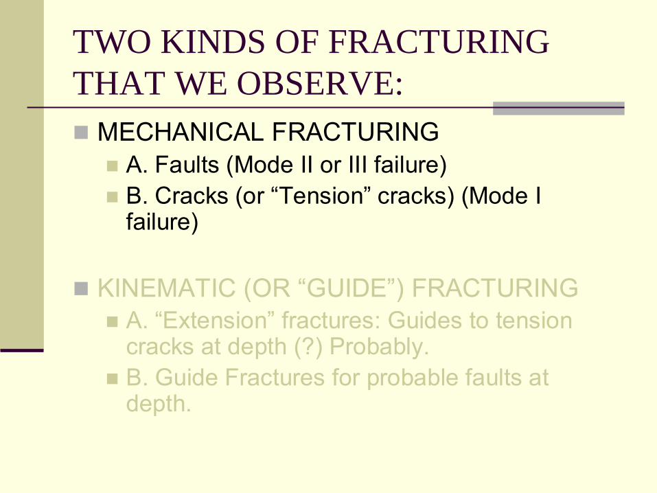
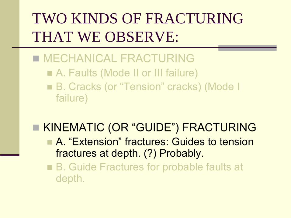
TWO KINDS OF FRACTURING THAT WE OBSERVE:
MECHANICAL FRACTURINGA. Faults (Mode II or III failure)B. Cracks (or “Tension” cracks) (Mode I failure)
KINEMATIC (OR “GUIDE”) FRACTURINGA. “Extension” fractures: Guides to tension cracks at depth (?) Probably.B. Guide Fractures for probable faults at depth.
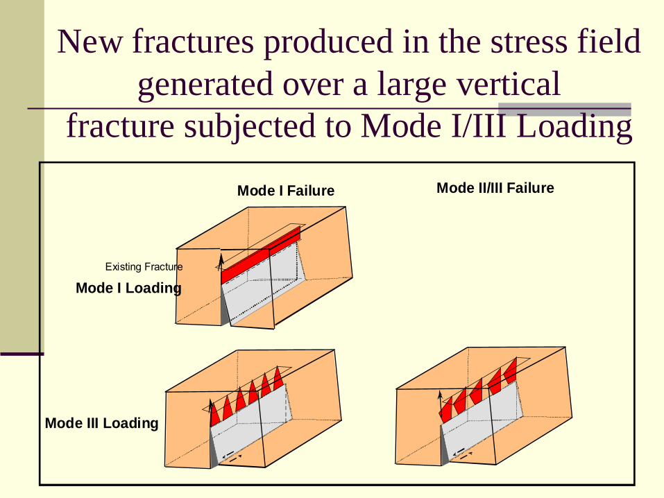
New fractures produced in the stress field generated over a large vertical
fracture subjected to Mode I/III Loading
Mode I Loading
Mode I Failure
Mode III Loading
Mode II/III Failure
Existing Fracture
FAULT SEGMENTS IN PIGPEN LANDSLIDE
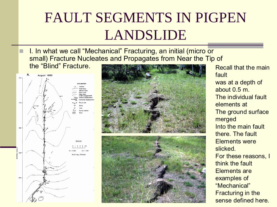
I. In what we call “Mechanical” Fracturing, an initial (micro or small) Fracture Nucleates and Propagates from Near the Tip of the “Blind” Fracture. Recall that the main
fault was at a depth of about 0.5 m.The individual fault elements atThe ground surface mergedInto the main fault there. The faultElements were slicked.For these reasons, I think the faultElements are examples of“Mechanical”Fracturing in thesense defined here.
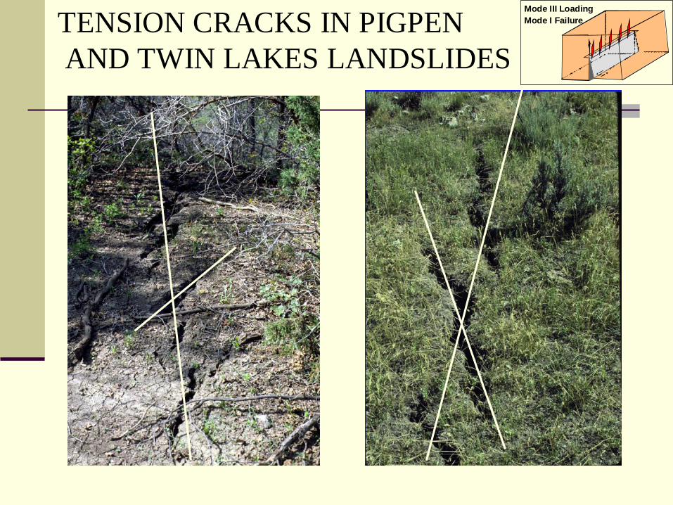
Mode I FailureMode III Loading
TENSION CRACKS IN PIGPENAND TWIN LAKES LANDSLIDES
Stress State Generated by a “Blind”Vertical Fracture, One with its
Tip Beneath Ground Surface
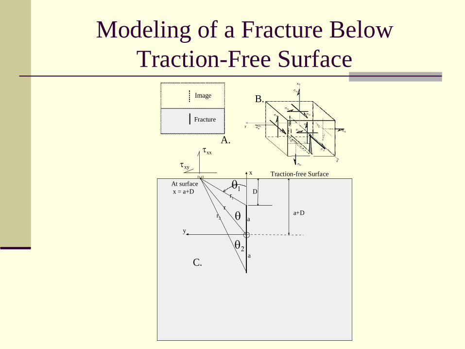
Modeling of a Fracture Below Traction-Free Surface
x
y
z
σxx
σyy
σyx
σ zz
σyz
σxy
σxz
σzy
σzx
σxx
σyy
D
x
y
r
r1
τxy
τxx
a
a
a+Dθ
At surface x = a+D
Traction-free Surface
r2
θ1
θ2
(x,y)
Fracture
Image
A.
B.
C.
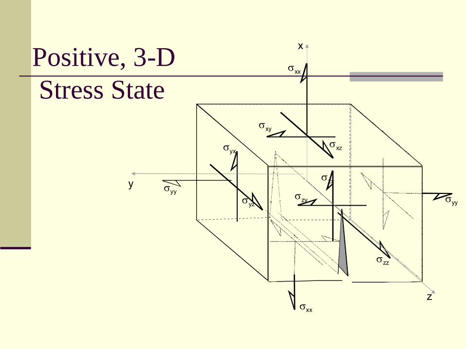
Positive, 3-DStress State
x
y
z
σxx
σyy
σyx
σzz
σyz
σxy
σxz
σzy
σzx
σxx
σyy
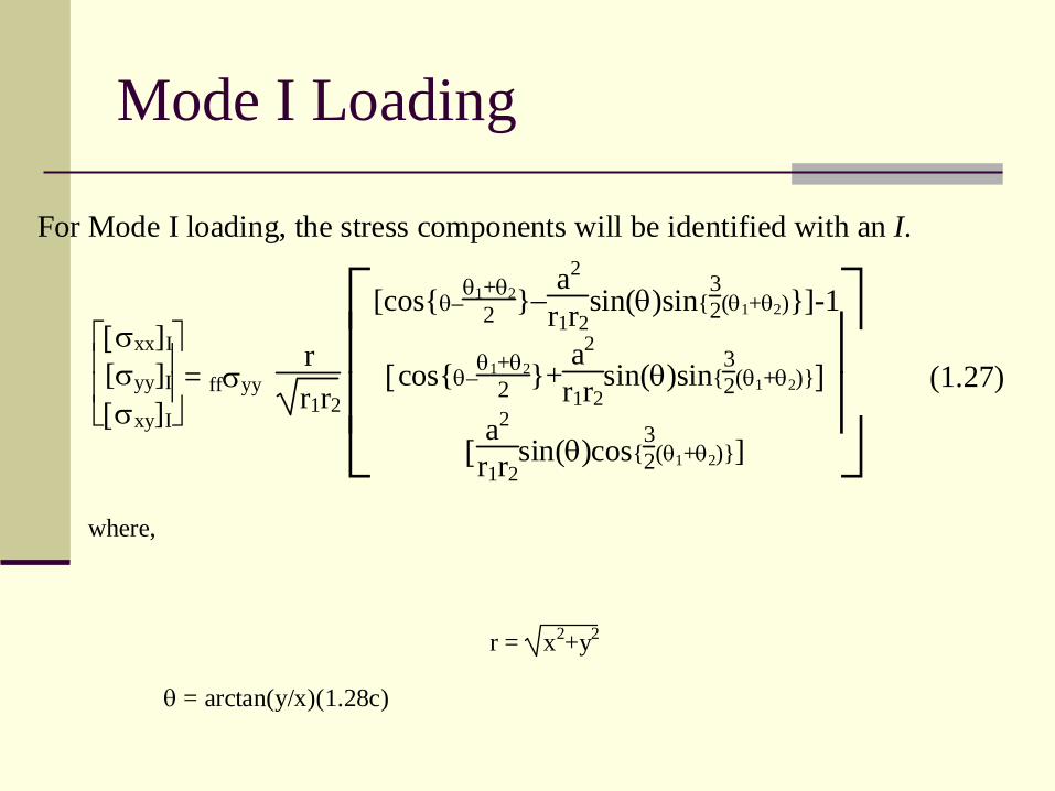
Mode I Loading
For Mode I loading, the stress components will be identified with an I.
⎣⎢⎢⎡
⎦⎥⎥⎤[σxx]I
[σyy]I
[σxy]I
= ffσyy rr1r2
⎣⎢⎢⎡
⎦⎥⎥⎤[cos{θ–
θ1+θ22 }−
a2
r1r2sin(θ)sin{
32(θ1+θ2)}]-1
[cos{θ–θ1+θ2
2 }+a2
r1r2sin(θ)sin{
32(θ1+θ2)}]
[a2
r1r2sin(θ)cos{
32(θ1+θ2)}]
(1.27)
where,
r = x2+y2
θ = arctan(y/x) (1.28c)
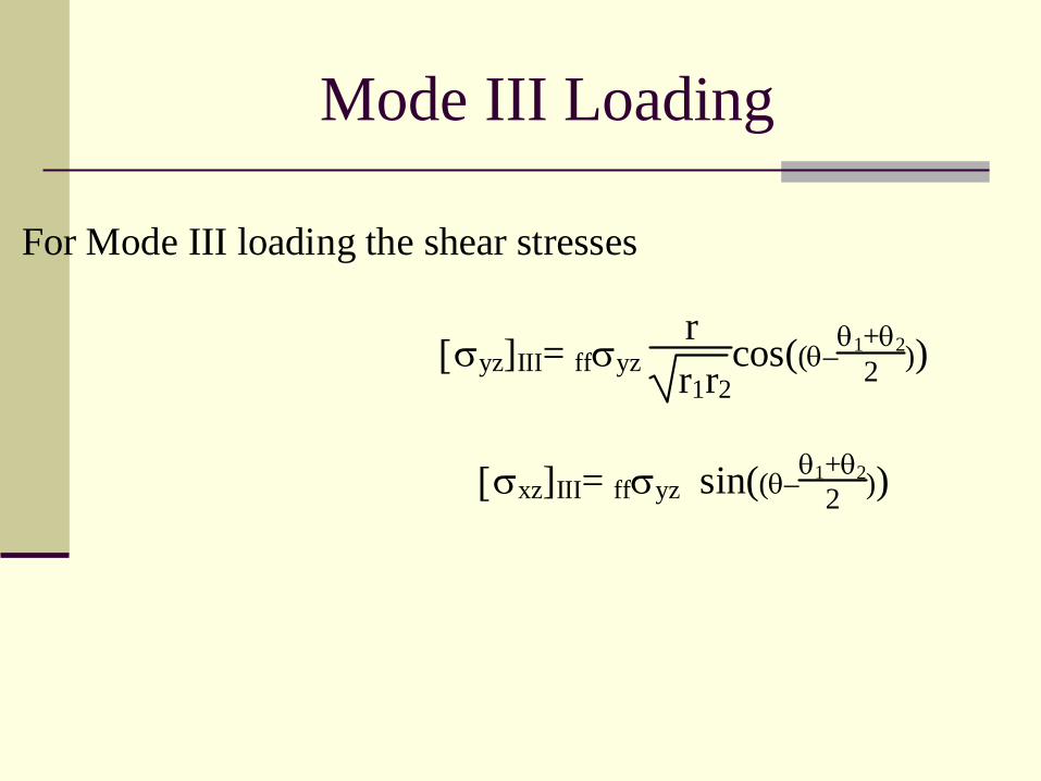
Mode III Loading
For Mode III loading the shear stresses
[σyz]III= ffσyz rr1r2
cos((θ–θ1+θ2
2 ))
[σxz]III= ffσyz sin((θ–θ1+θ2
2 ))
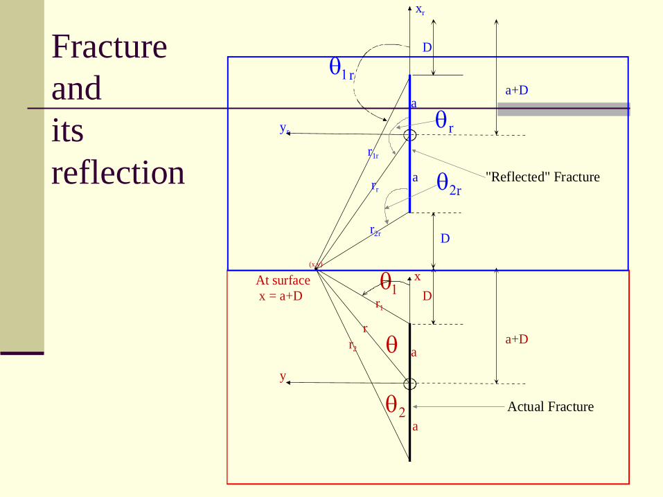
Fracture andits reflection
Dx
y
r
r1
a
a
a+Dθ
At surface x = a+D
r2
θ1
θ2
(x,y)
D
xr
yr
rr
r1r
a
a
a+D
θr
r2r
θ1r
θ2r
D
"Reflected" Fracture
Actual Fracture
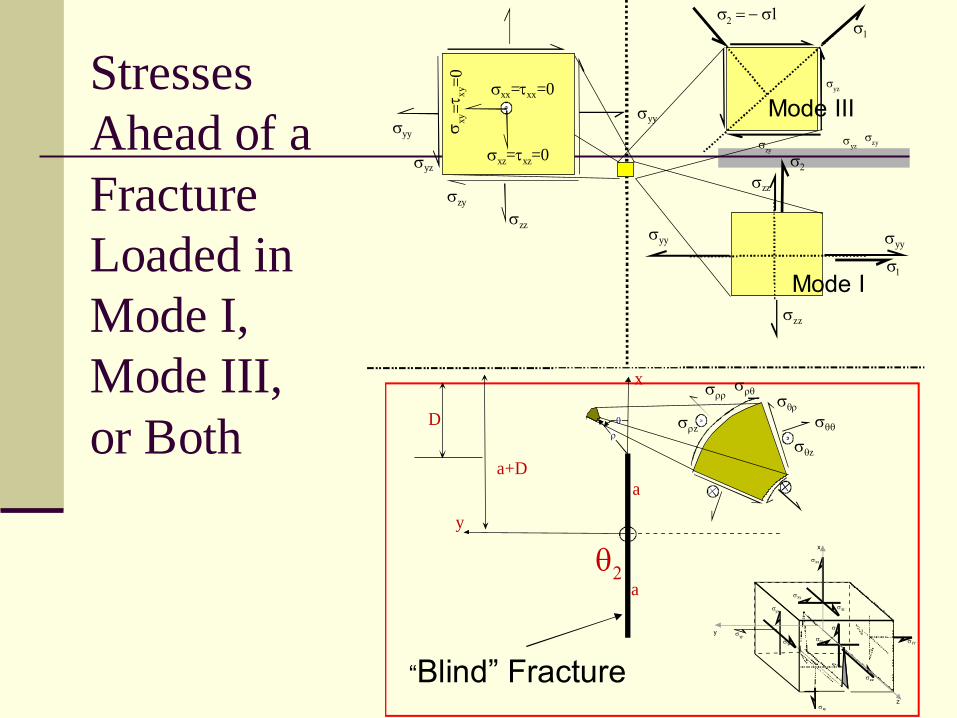
StressesAhead of aFractureLoaded inMode I,Mode III,or Both D
x
y
a
a
a+D
θ2
ρθ σθθ
σρρ σθρ
σρθ
σρz
σθz
x
y
z
σxx
σyy
σyx
σzz
σyz
σxy
σxz
σzy
σzx
σxx
σyy
σyz
σzy
σzz
σyy
σyz
σzy
σyy
σ1
σ2 = − σ1
σxx=τxx=0
σxz=τxz=0
σ xy=τ
xy=0
σyzσzy
σ1
σ2
σyyσyy
σzz
σzz
“Blind” Fracture
Mode I
Mode III
“Mechanical Fracturing” Cont’I. In what we call “Mechanical” Fracturing, an initial (micro or small) Fracture Nucleates and Propagates from Near the Tip of the “Blind”Fracture.
This kind of fracturing is perhaps best analyzed with linear-fracture mechanics.One compares the1) Stress-Intensity Factor, KI or KIII (or KII), for a microfracture within the stress field generated by the tip of the main fracture2) to the Critical Stress-intensity Factor, KIc or KIIIc, for the material containing the microfracture. The critical stress-intensity factor is considered to be a property of the material containing the main fracture.
TWO KINDS OF FRACTURING THAT WE OBSERVE:
MECHANICAL FRACTURINGA. Faults (Mode II or III failure)B. Cracks (or “Tension” cracks) (Mode I failure)
KINEMATIC (OR “GUIDE”) FRACTURINGA. “Extension” fractures: Guides to tension cracks at depth (?) Probably.B. Guide Fractures for probable faults at depth.
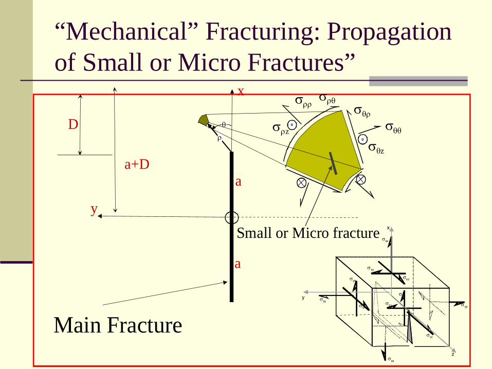
“Mechanical” Fracturing: Propagation of Small or Micro Fractures”
D
x
y
a
a
a+D
ρ
θ σθθ
σρρ σθρ
σρθ
σρz
σθz
x
y
z
σxx
σyy
σyx
σzz
σyz
σxy
σxz
σzy
σzx
σxx
σyy
Main Fracture
Small or Micro fracture
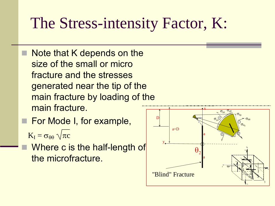
The Stress-intensity Factor, K:
Note that K depends on the size of the small or micro fracture and the stresses generated near the tip of the main fracture by loading of the main fracture.For Mode I, for example,
Where c is the half-length of the microfracture.
D
x
y
a
a
a+D
θ2
ρ
θ σθθ
σρρ σθρ
σρθ
σρz
σθz
x
y
z
σxx
σyy
σyx
σzz
σy z
σxy
σx z
σzy
σzx
σxx
σyy
"Blind" Fracture
KI = σθθ πc
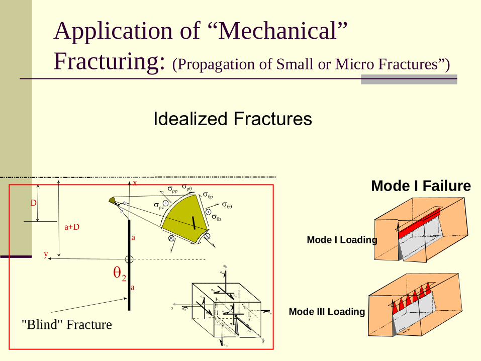
Application of “Mechanical”Fracturing: (Propagation of Small or Micro Fractures”)
D
x
y
a
a
a+D
θ2
ρ
θ σθθ
σρρ σθρ
σρθ
σρz
σθz
x
y
z
σxx
σyy
σyx
σzz
σyz
σxy
σxz
σzy
σzx
σxx
σyy
"Blind" Fracture
Mode I Loading
Mode I Failure
Mode III Loading
Idealized Fractures
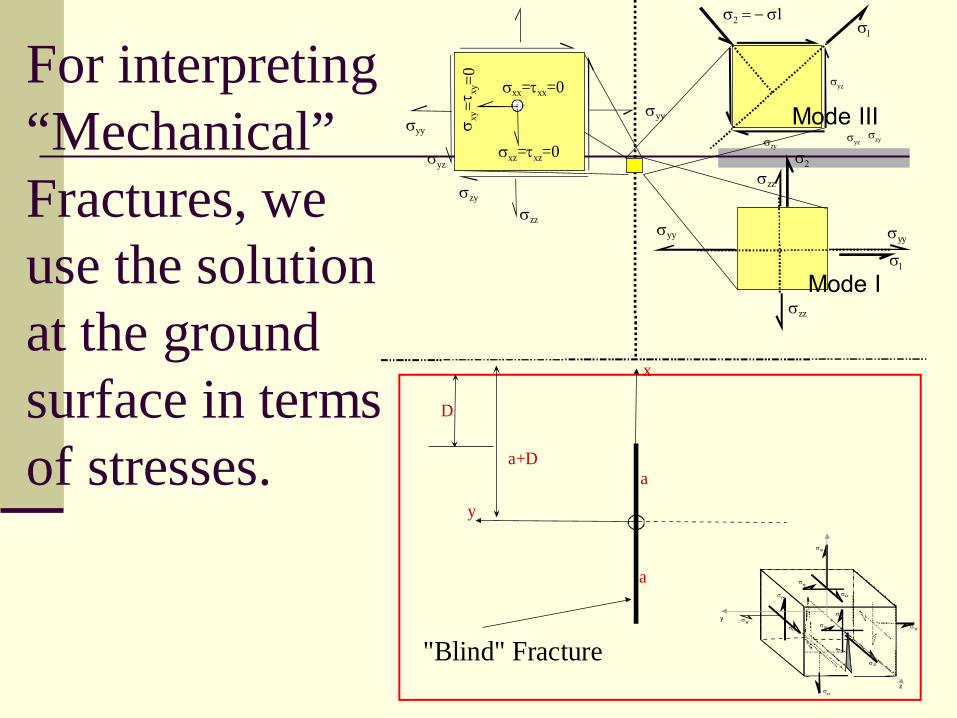
For interpreting “Mechanical”Fractures, we use the solution at the ground surface in terms of stresses.
D
x
y
a
a
a+D
y
z
σxx
σyy
σyx
σzz
σyz
σxy
σxz
σzy
σzx
σxx
σyy
σyz
σzy
σzz
σyy
σyz
σzy
σyy
σ1
σ2 = − σ1
σxx=τxx=0
σxz=τxz=0
σ xy=τ
x y=0
σyzσzy
σ1
σ2
σyyσyy
σzz
σzz
"Blind" Fracture
Mode I
Mode III
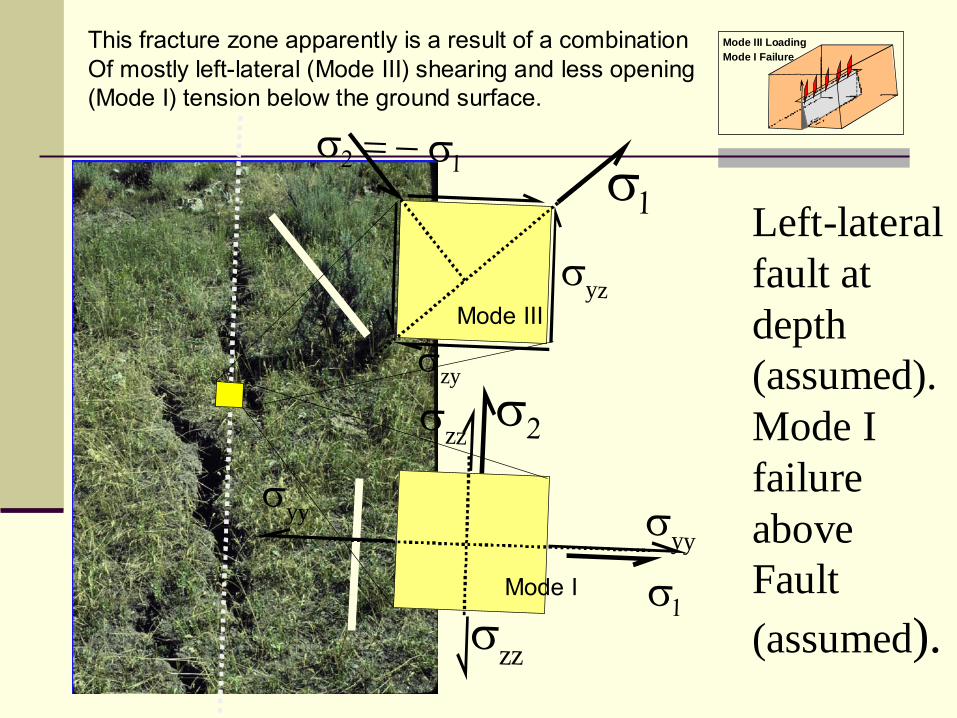
Left-lateral fault at depth (assumed). Mode I failure aboveFault (assumed).
Mode I FailureMode III Loading
σyz
σzy
σ1
σ2 = − σ1
σ1
σ2
σyy
σyy
σzz
σzz
This fracture zone apparently is a result of a combinationOf mostly left-lateral (Mode III) shearing and less opening(Mode I) tension below the ground surface.
Mode I
Mode III
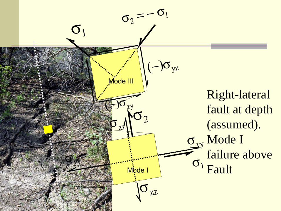
Right-lateral fault at depth (assumed). Mode I failure aboveFault
(−)σyz
(−)σzy
σ1σ2 = − σ1
σ1
σ2
σyy
σyy
σzz
σzz
Mode I
Mode III
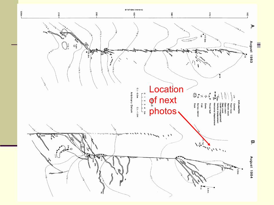
Map of Fractures at Ground Surface
Location of nextphotos
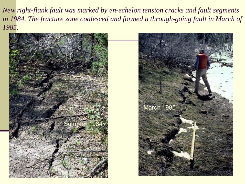
New right-flank fault was marked by en-echelon tension cracks and fault segments in 1984. The fracture zone coalesced and formed a through-going fault in March of 1985.
Summer 1984
March 1985
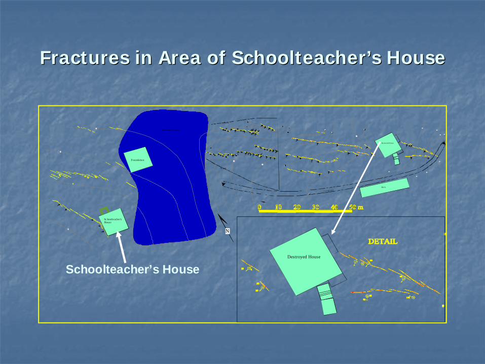
Fractures in Area of SchoolteacherFractures in Area of Schoolteacher’’s Houses House
N
Destroyed House
20
30
30
20
22
1 0
3
20
20
10
10
3
2
40
10
1010
15
5
5
5
5
2 0
3 0
20
40
Barn
De st royed House
Gr avel Dr iv ew ay
10 3
-5
-6
-6
-7
-7
-8
-8
-55
5
40
36
5 8 2227
9
1 0
1 010
10
1 0
5
9
0130
99
50
78
9
10 2 1 023
132
6
4
16
3
25 6 15
1 6
13
2514
211 0
1 0
43
12
20
20
50
5
2510
3010
2 0
8
30
54
85
75
10
1 0
20
20
2
Sc hoolteacher'sHouse
Fou ndatio n1 20
- 2
-1
-3
1
2
4
Distur be d Gro un d
fence
fen ce
Schoolteacher’s House
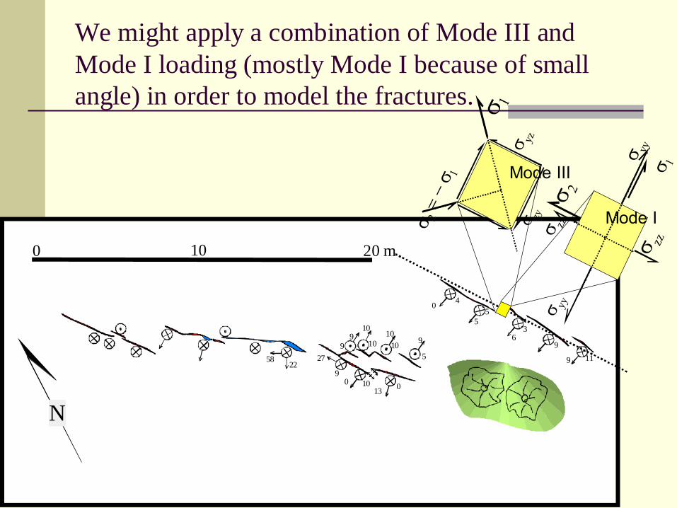
We might apply a combination of Mode III and Mode I loading (mostly Mode I because of small angle) in order to model the fractures.
0 10 20 m
N
119
9
55
40
36
5822
27
9
10
1010
10
10
5
9
0130
99
σ yzσ zy
σ 1
σ 2 =
− σ 1 σ 1
σ 2
σ yy
σ yy
σ zz
σ zz Mode I
Mode III
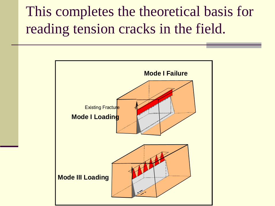
This completes the theoretical basis for reading tension cracks in the field.
Mode I Loading
Mode I Failure
Mode III Loading
Existing Fracture
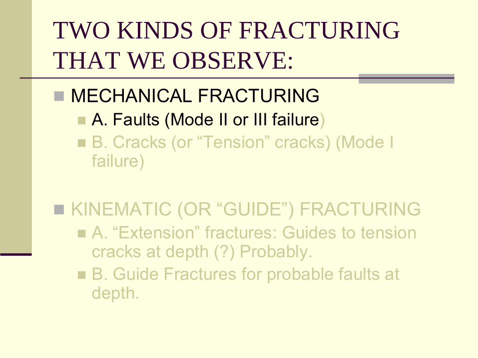
TWO KINDS OF FRACTURING THAT WE OBSERVE:
MECHANICAL FRACTURINGA. Faults (Mode II or III failure)B. Cracks (or “Tension” cracks) (Mode I failure)
KINEMATIC (OR “GUIDE”) FRACTURINGA. “Extension” fractures: Guides to tension cracks at depth (?) Probably.B. Guide Fractures for probable faults at depth.
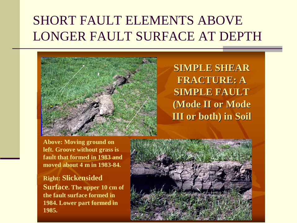
SHORT FAULT ELEMENTS ABOVE LONGER FAULT SURFACE AT DEPTH
SIMPLE SHEAR SIMPLE SHEAR FRACTURE: A FRACTURE: A
SIMPLE FAULT SIMPLE FAULT (Mode II or Mode (Mode II or Mode III or both) in SoilIII or both) in Soil
Above: Moving ground on left. Groove without grass is fault that formed in 1983 and moved about 4 m in 1983-84.
Right: SlickensidedSurface. The upper 10 cm of the fault surface formed in 1984. Lower part formed in 1985.
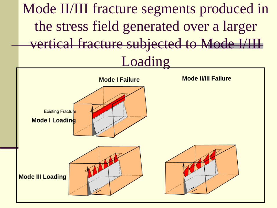
Mode II/III fracture segments produced in the stress field generated over a larger
vertical fracture subjected to Mode I/III Loading
Mode I Loading
Mode I Failure
Mode III Loading
Mode II/III Failure
Existing Fracture
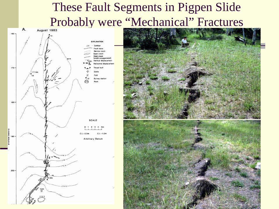
These Fault Segments in Pigpen Slide Probably were “Mechanical” Fractures
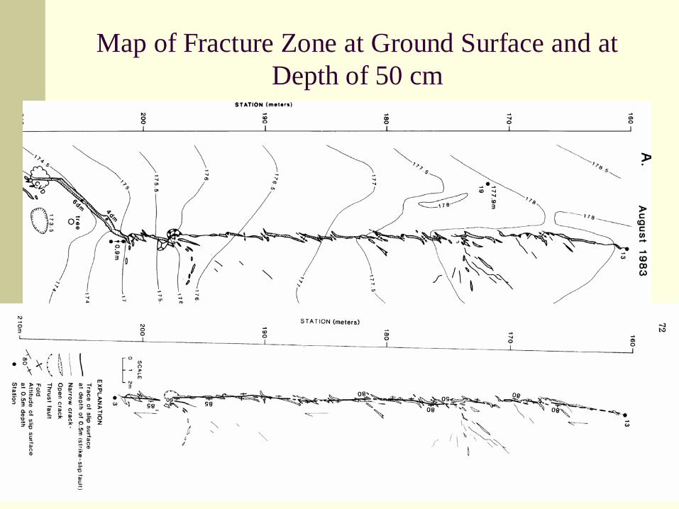
Map of Fracture Zone at Ground Surface and at Depth of 50 cm
A possible explanation for the short fault segments being differently oriented from longer faults below.
Theoretical Interlude
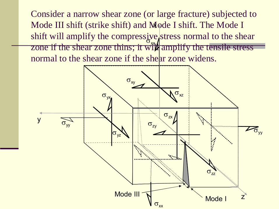
Consider a narrow shear zone (or large fracture) subjected to Mode III shift (strike shift) and Mode I shift. The Mode I shift will amplify the compressive stress normal to the shear zone if the shear zone thins; it will amplify the tensile stressnormal to the shear zone if the shear zone widens.
x
y
z
σxx
σyy
σyx
σzz
σyz
σxy
σxz
σzy
σzx
σxx
σyy
Mode IIIMode I
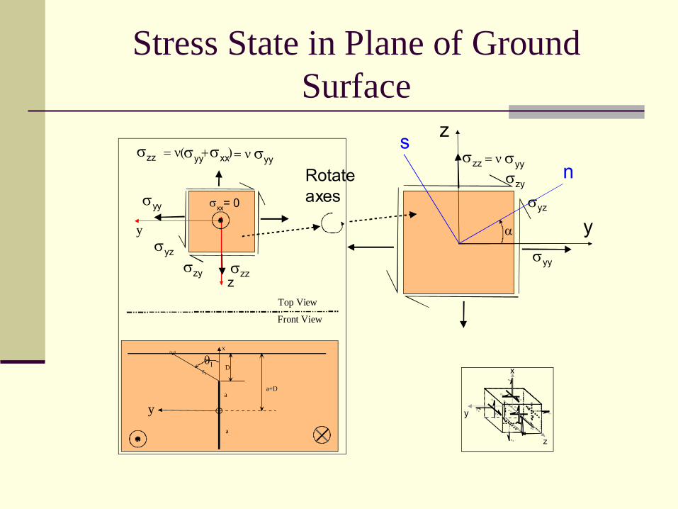
Stress State in Plane of Ground Surface
x
y
z
σxx
σ yy
σyx
σzz
σ yz
σ xy
σ xz
σ zy
σzx
σ xx
σyy
D
x
y
r1
a
a
a+D
θ1
(x,y)
σzz
σyy
σyz
σxx= 0
σzy
y
Top View
Front View
z
σzz = ν( + )σxxσyy = ν σyy
σyy
σyz
σzy
y
zσzz = ν σyy n
s
α
Rotateaxes
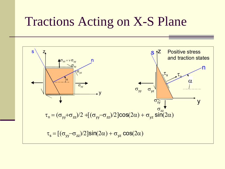
Tractions Acting on X-S Plane
σyy
σyz
σzy
y
zσzz = ν σyy n
s
α
σyy σyz
σzy y
z
σzz
τs
n
s
ατn
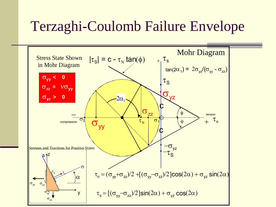
τn = (σyy+σzz)/2 +[(σyy−σzz)/2]cos(2α) + σyz sin(2α)
τs = [(σyy−σzz)/2]sin(2α) + σyz cos(2α)
Positive stressand traction states
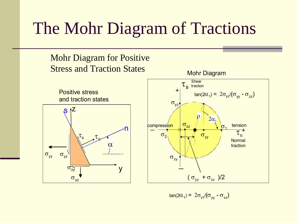
The Mohr Diagram of Tractions
τs
τn
−
tensioncompression−
σyy
σzz σ1
σ2
2α1
Sheartraction
Normaltraction
σyz
σzy
( σyy + σzz )/2
ρ
tan(2α1) = 2σyz/(σyy - σzz)
σyy σyz
σzy y
z
σzz
τs
n
s
ατn
Positive stressand traction states
Mohr Diagram for PositiveStress and Traction States Mohr Diagram
+
tan(2α1) = 2σyz/(σyy - σzz)
+
Terzaghi-Coulomb Failure Envelope
σyy σyz
σzy y
z
σzz
τs
n
s
ατn τn = (σyy+σzz)/2 +[(σyy−σzz)/2]cos(2α) + σyz sin(2α)
τs = [(σyy−σzz)/2]sin(2α) + σyz cos(2α)
τs
τn
−
tension
compression
−
+
c
c+σyy
σzzτΝ
σyz
−σyz
σ2 σ1
σzz = νσyy
σyy < 0 τS
τS
φ
|τS| = c - τΝ tan(φ)
Stresses and Tractions for Positive States
σyz > 0
Stress State Shown in Mohr Diagram
Mohr Diagram
tan(2α1) = 2σyz/(σyy - σzz)
2α1
Solution for Orientation of Left-Lateral Fault Segments
σyy σyz
σzy y
z
σzz
τs
n
s
ατn
σzz = νσyy
σyy < 0
Stresses and Tractions for Positive States
σyz > 0
Stress State Shown in Mohr Diagram
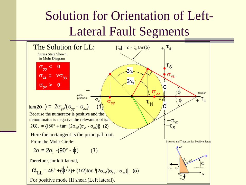
The Solution for LL: τs
τn
−
tensioncom-pression
−
+
2α
+σyy
σzz
τΝ
σyz
−σyz
σ2σ1
τS
τS
φ
|τS| = c - τΝ tan(φ)
2α1
c
c
tan(2α1) = 2σyz/(σyy - σzz) (1)
2α1 = {180° + tan-1[2σyz/(σyy - σzz)]} (2)
2α = 2α1 -(90° - φ) (3)From the Mohr Circle:
Therefore, for left-lateral,
αLL = 45° +(φ/2)+ (1/2)tan-1[2σyz/(σyy - σzz)] (5)
Because the numerator is positive and thedenominator is negative the relevant root is:
Here the arctangent is the principal root.
For positive mode III shear.(Left lateral).
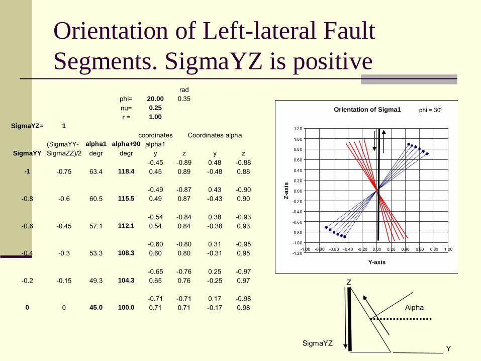
Orientation of Left-lateral Fault Segments. SigmaYZ is positive
radphi= 20.00 0.35nu= 0.25r = 1.00
SigmaYZ= 1coordinates Coordinates alpha
(SigmaYY- alpha1 alpha+90 alpha1SigmaYY SigmaZZ)/2 degr degr y z y z
-0.45 -0.89 0.48 -0.88-1 -0.75 63.4 118.4 0.45 0.89 -0.48 0.88
-0.49 -0.87 0.43 -0.90-0.8 -0.6 60.5 115.5 0.49 0.87 -0.43 0.90
-0.54 -0.84 0.38 -0.93-0.6 -0.45 57.1 112.1 0.54 0.84 -0.38 0.93
-0.60 -0.80 0.31 -0.95-0.4 -0.3 53.3 108.3 0.60 0.80 -0.31 0.95
-0.65 -0.76 0.25 -0.97-0.2 -0.15 49.3 104.3 0.65 0.76 -0.25 0.97
-0.71 -0.71 0.17 -0.980 0 45.0 100.0 0.71 0.71 -0.17 0.98
Orientation of Sigma1
-1.20
-1.00
-0.80
-0.60
-0.40
-0.20
0.00
0.20
0.40
0.60
0.80
1.00
1.20
-1.00 -0.80 -0.60 -0.40 -0.20 0.00 0.20 0.40 0.60 0.80 1.00
Y-axis
Z-ax
is
phi = 30°
Alpha
SigmaYZY
Z
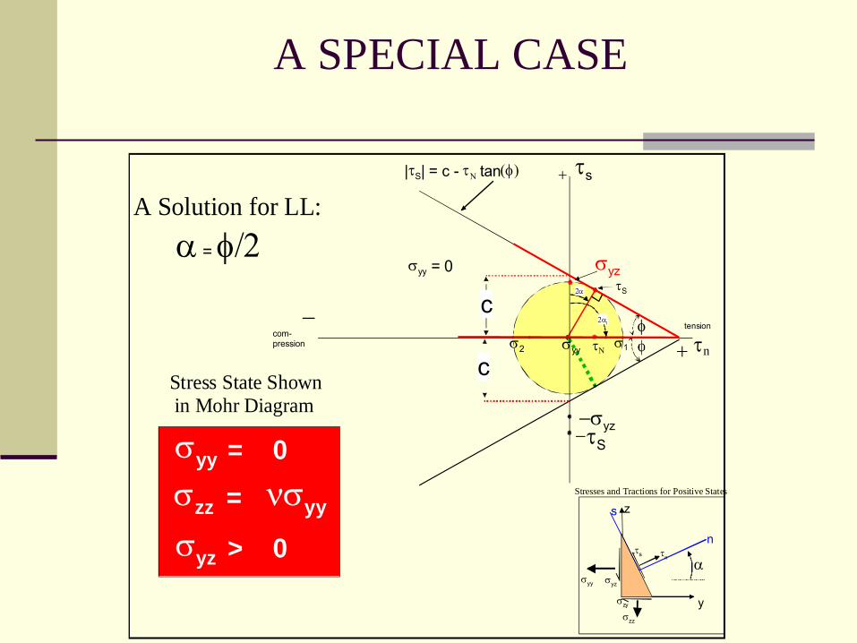
A SPECIAL CASE
2α
τΝσ1
2α1
σyy σyz
σzy y
z
σzz
τs
n
s
ατn
σzz = νσyy
σyy = 0Stresses and Tractions for Positive States
σyz > 0
Stress State Shown in Mohr Diagram
A Solution for LL:τs
τn
−
tensioncom-pression
−
+
+
σyz
−σyz
σ2
τS
τS
φ
|τS| = c - τΝ tan(φ)
c
c
σyy = 0
σyy
α = φ/2
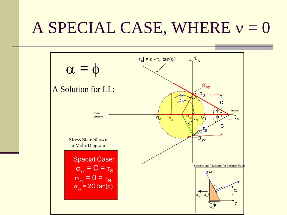
A SPECIAL CASE, WHERE ν = 0
2α
τΝσ1
2α1
α
σyy σyz
σzy y
z
σzz
τs
n
s
ατn
Stresses and Tractions for Positive States
Stress State Shown in Mohr Diagram
A Solution for LL:
τs
τn
−
tensioncom-pression
−
+
+
σyz
−σyz
σ2
τS
τS
φ
|τS| = c - τΝ tan(φ)
c
c
σyyσzz
Special Case:
σzz = 0 = τN
σyz = C = τS
σyy = 2C tan(φ)
α = φ
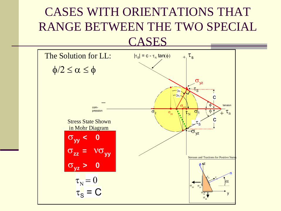
CASES WITH ORIENTATIONS THAT RANGE BETWEEN THE TWO SPECIAL
CASES
2α
τΝσ1
2α1
σyy σyz
σzy y
z
σzz
τs
n
s
ατn
σzz = νσyy
σyy < 0
Stresses and Tractions for Positive States
σyz > 0
Stress State Shown in Mohr Diagram
The Solution for LL: τs
τn
−
tensioncom-pression
−
+
+
σyz
−σyz
σ2
τS
τS
φ
|τS| = c - τΝ tan(φ)
c
c
σyy
σzz
φ/2 ≤ α ≤ φ
τS = CτΝ = 0
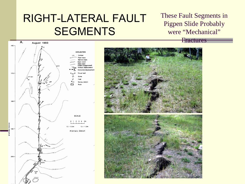
These Fault Segments in Pigpen Slide Probably
were “Mechanical”Fractures
RIGHT-LATERAL FAULT SEGMENTS
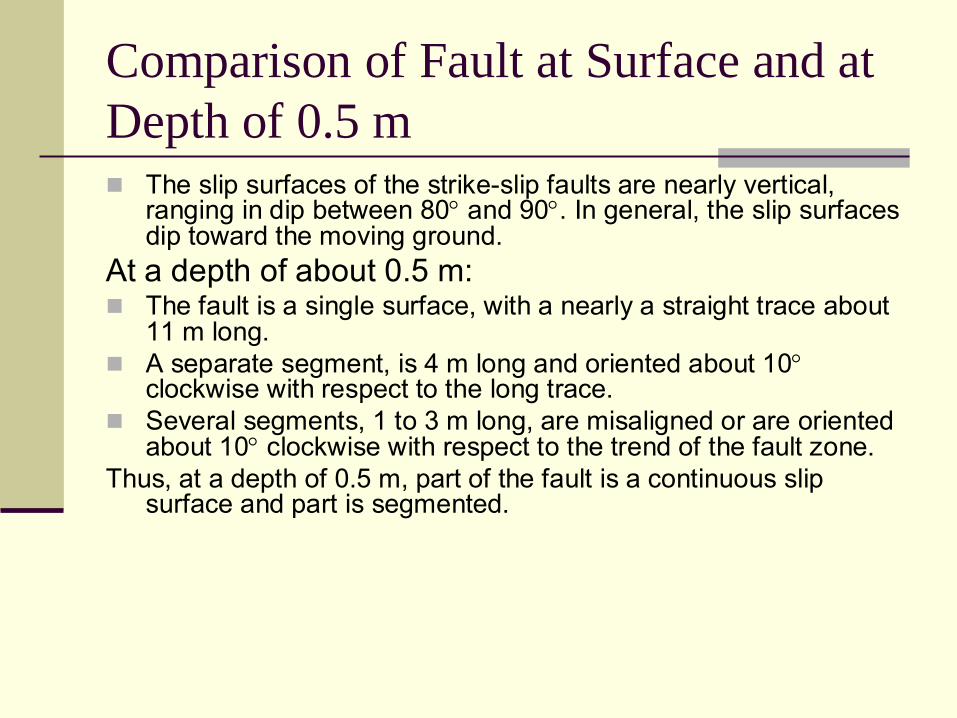
Comparison of Fault at Surface and at Depth of 0.5 m
The slip surfaces of the strike-slip faults are nearly vertical, ranging in dip between 80° and 90°. In general, the slip surfaces dip toward the moving ground.
At a depth of about 0.5 m: The fault is a single surface, with a nearly a straight trace about 11 m long.A separate segment, is 4 m long and oriented about 10°clockwise with respect to the long trace.Several segments, 1 to 3 m long, are misaligned or are oriented about 10° clockwise with respect to the trend of the fault zone.
Thus, at a depth of 0.5 m, part of the fault is a continuous slip surface and part is segmented.
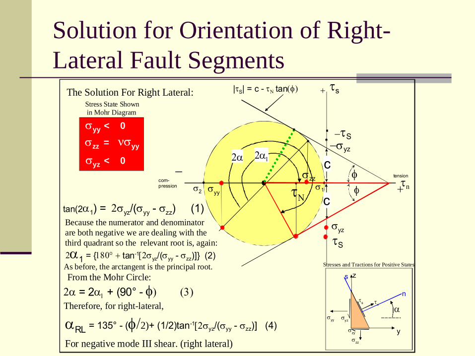
Solution for Orientation of Right-Lateral Fault Segments
σyy σyz
σzy y
z
σzz
τs
n
s
ατn
σzz = νσyy
σyy < 0
Stresses and Tractions for Positive States
σyz < 0
Stress State Shown in Mohr Diagram
The Solution For Right Lateral: τs
τn
−
tensioncom-pression
−
+
+σyy
σzz
τΝ
σyz
−σyz
σ2σ1
τS
τS
φ
|τS| = c - τΝ tan(φ)
2α1
c
c
tan(2α1) = 2σyz/(σyy - σzz) (1)
2α1 = {180° + tan-1[2σyz/(σyy - σzz)]} (2)
2α = 2α1 + (90° - φ) (3)From the Mohr Circle:
Therefore, for right-lateral,
αRL = 135° - (φ/2)+ (1/2)tan-1[2σyz/(σyy - σzz)] (4)
Because the numerator and denominatorare both negative we are dealing with thethird quadrant so the relevant root is, again:
As before, the arctangent is the principal root.
For negative mode III shear. (right lateral)
2α
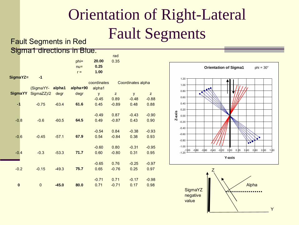
Orientation of Right-LateralFault Segments
Fault Segments in RedSigma1 directions in Blue.
radphi= 20.00 0.35nu= 0.25r = 1.00
SigmaYZ= -1coordinates Coordinates alpha
(SigmaYY- alpha1 alpha+90 alpha1SigmaYY SigmaZZ)/2 degr degr y z y z
-0.45 0.89 -0.48 -0.88-1 -0.75 -63.4 61.6 0.45 -0.89 0.48 0.88
-0.49 0.87 -0.43 -0.90-0.8 -0.6 -60.5 64.5 0.49 -0.87 0.43 0.90
-0.54 0.84 -0.38 -0.93-0.6 -0.45 -57.1 67.9 0.54 -0.84 0.38 0.93
-0.60 0.80 -0.31 -0.95-0.4 -0.3 -53.3 71.7 0.60 -0.80 0.31 0.95
-0.65 0.76 -0.25 -0.97-0.2 -0.15 -49.3 75.7 0.65 -0.76 0.25 0.97
-0.71 0.71 -0.17 -0.980 0 -45.0 80.0 0.71 -0.71 0.17 0.98
Orientation of Sigma1
-1.20
-1.00
-0.80
-0.60
-0.40
-0.20
0.00
0.20
0.40
0.60
0.80
1.00
1.20
-1.00 -0.80 -0.60 -0.40 -0.20 0.00 0.20 0.40 0.60 0.80 1.00
Y-axis
Z-ax
is
phi = 30°
AlphaSigmaYZnegativevalue
Y
Z
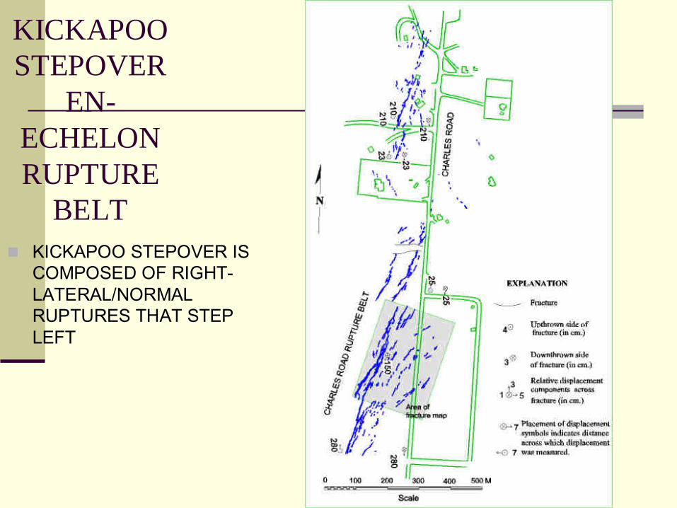
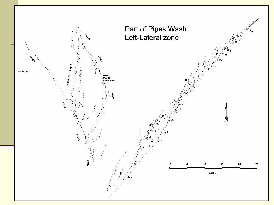
KICKAPOO STEPOVER
EN-ECHELON RUPTURE
BELTKICKAPOO STEPOVER IS COMPOSED OF RIGHT-LATERAL/NORMAL RUPTURES THAT STEP LEFT
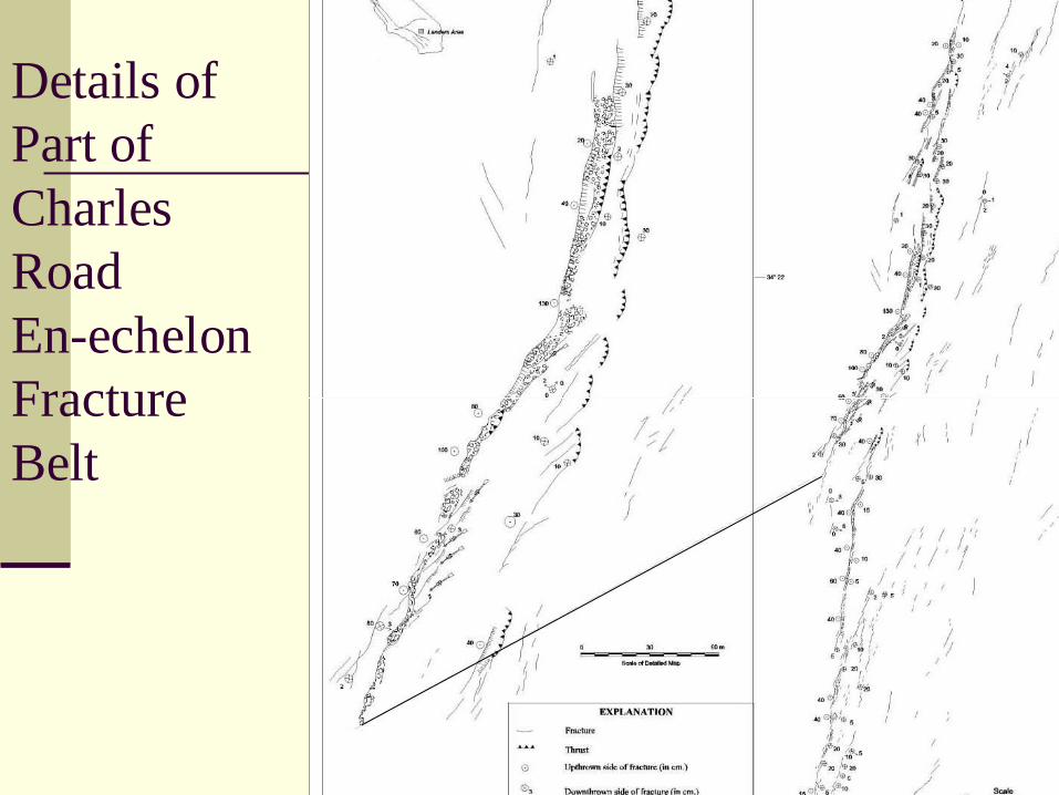
Details ofPart of CharlesRoadEn-echelonFractureBelt
6
HE
ADQ
UA
RTE
RS
DU
PL E
XS
TRU
CT
UR
E
MAPPED IN AUGUST 1993
32
6
NO RTHERN RANCH
MILESKA RANCH
HEA D
QUA
RTE
R SD U
PLEX
STRU
CTUR
E
BODICK
ROAD
NO T MAPPED
NOT MAPPE D
NOT MAPPED
NO CRACKS
NO CRACKS
5
6
3
MAPPED IN J ULY 1992
MAPPED IN AUG UST 1993
MAPPED IN AUGUST 1993
MAPPED IN AUG UST 1993
EXPLANATION
Fract ure
Tensio n Crack (sc hemat ic)
Th ru st
Upt hrown Side o f Fract ure (cm)
Do wn thrown Side of Fractu re (cm)
5 Rela tiv e Di sp lacement Co mp one nts across Fractu re(vertic al =2 cm, la teral = 7 cm, o pen ing = 5 cm)
Compon ent of Di sp lacemen t of Fence Po st No rmalto Fen ce Line (cm)
45
MIKISKA BOULEVARD
CALI FORNIA
L an de rs Are a
HOMESTEAD
F AU L T
VA L LE Y
JOHNSONVA L LE Y
F AUL TZONE
Z ON E
K ICKA
POO
F AUL
T
AREAOF
MAP
SHAW
NEE
ROAD NOT
MAPPED
3 4° 22 ' 2 2"
1 16 °
30'
1 16 °
30'3 4° 23 '
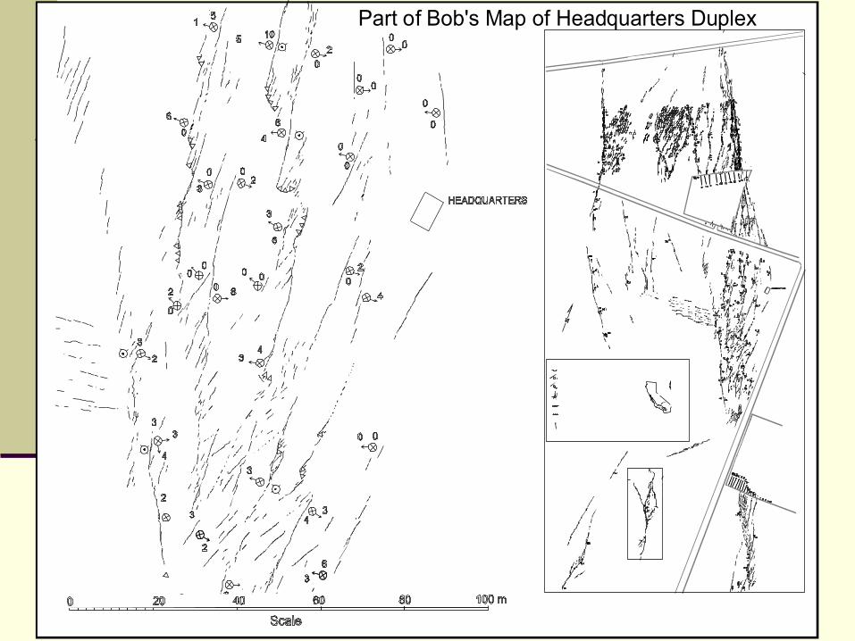
Part of Bob's Map of Headquarters DuplexPart of Bob's Map of Headquarters Duplex
This Completes the Discussion ofMechanical Fracturing
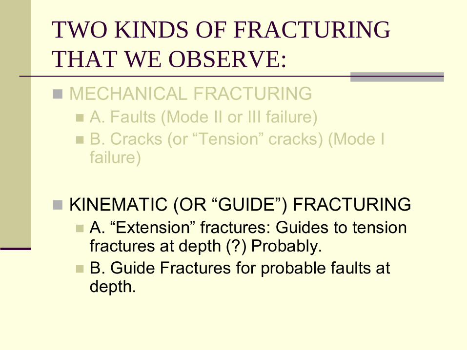
TWO KINDS OF FRACTURING THAT WE OBSERVE:
MECHANICAL FRACTURINGA. Faults (Mode II or III failure)B. Cracks (or “Tension” cracks) (Mode I failure)
KINEMATIC (OR “GUIDE”) FRACTURINGA. “Extension” fractures: Guides to tension fractures at depth (?) Probably.B. Guide Fractures for probable faults at depth.

II. “Kinematic” Fracturing
In what we call “Kinematic” fracturing ( perhaps a better term is “Guide” fracturing), highly irregular gashes appear in soil at the ground surface.
1). The pattern of the fractures and related structures appear to be controlled by details of irregular cracks or other irregularities in the compact soil.2). We call these “Guide Fractures.” They are results of extension or shearing deformation (not high stress!) at the ground surface probably caused by a “Blind” fracture below.
This kind of fracturing cannot be analyzed with linear-fracture mechanics.
1). One cannot recognize planar or curviplanar discontinuities that one would consider, mechanically, to behave as fractures.Thus, in this case we do not read the stress state. We read the deformation state.
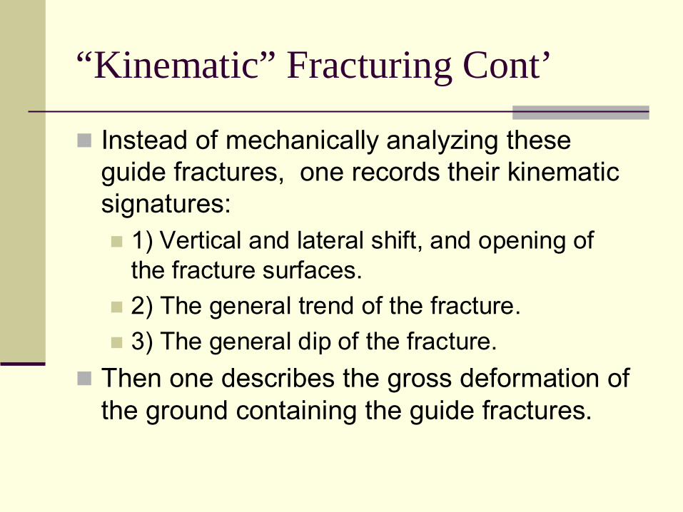
“Kinematic” Fracturing Cont’
Instead of mechanically analyzing these guide fractures, one records their kinematicsignatures:
1) Vertical and lateral shift, and opening of the fracture surfaces.2) The general trend of the fracture.3) The general dip of the fracture.
Then one describes the gross deformation of the ground containing the guide fractures.
TWO KINDS OF FRACTURING THAT WE OBSERVE:
MECHANICAL FRACTURINGA. Faults (Mode II or III failure)B. Cracks (or “Tension” cracks) (Mode I failure)
KINEMATIC (OR “GUIDE”) FRACTURINGA. “Extension” fractures: Guides to tension fractures at depth. (?) Probably.B. Guide Fractures for probable faults at depth.
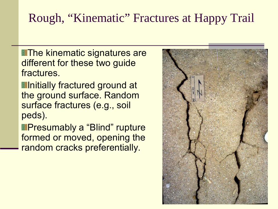
Rough, “Kinematic” Fractures at Happy Trail
The kinematic signatures are different for these two guide fractures.
Initially fractured ground at the ground surface. Random surface fractures (e.g., soil peds).
Presumably a “Blind” rupture formed or moved, opening the random cracks preferentially.
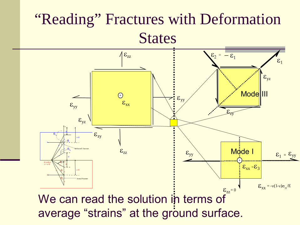
“Reading” Fractures with Deformation States
εyy
εyz
εzy
εzz
εxxεyy
εzz
εyy εyyε1
εzy
εyz
ε2 ε1
= − ε1
εxx = ε3
εxx = -ν(1-ν)σyy/Eεzz= 0
=
We can read the solution in terms ofaverage “strains” at the ground surface.
Dx
y
r
r1
a
a
a+Dθ
At surface x = a+D
r2
θ1
θ2
(x,y )
D
xr
yr
rr
r1 r
a
a
a+D
θr
r2 r
θ1r
θ2r
D
"Reflected" Fracture
Actual Fracture
Mode III
Mode I
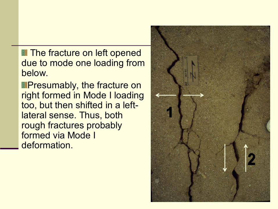
The fracture on left opened due to mode one loading from below.
Presumably, the fracture on right formed in Mode I loading too, but then shifted in a left-lateral sense. Thus, both rough fractures probably formed via Mode I deformation.
Some Comments on “Kinematic” Fractures. Also known as “Guide Fractures.”
It is presumably important to bear in mind that the general orientation of the highly irregular trace and surfaces of the guide fracture that we observe at the ground surface is controlled by the orientation of the fracture (or fracture zone) that occurs below, in the shallow subsurface.The opening of the guide fracture is a result of “strains produced by the subsurface fracture.The orientation of the subsurface fractures, below the guide fractures, presumably, is controlled by the stress state at the depth of the subsurface fractures.Thus we consider the general trend of the guide fractures at the ground surface to reflect the general trend of the subsurface fracture (or fracture zone).
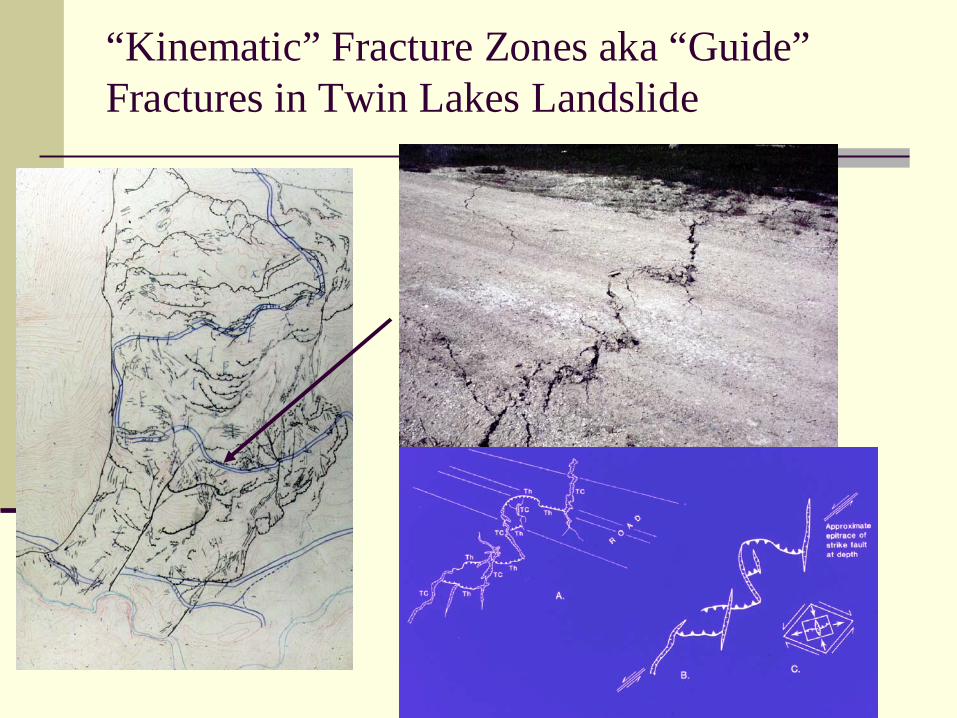
“Kinematic” Fracture Zones aka “Guide”Fractures in Twin Lakes Landslide
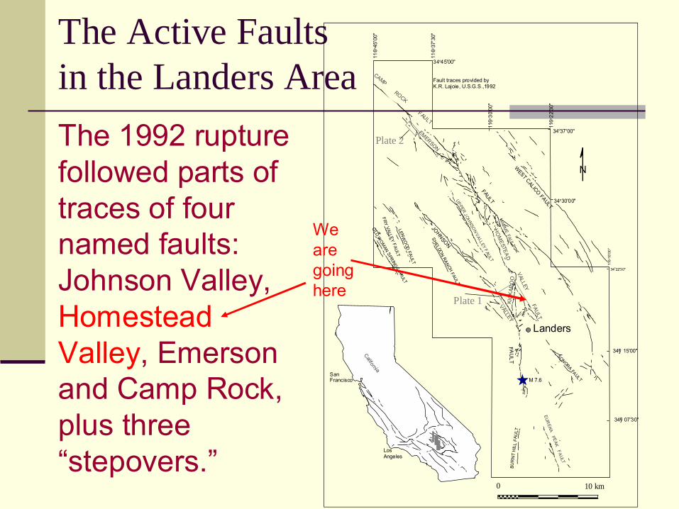
The Active Faults in the Landers Area
34ºÿ 07'30"
34ºÿ 15'00"
34o22'30"
116o
15'0
0"
34o30'00"
34o37'00"
116o
22'3
0"
116o
30'0
0"
116o
45'0
0"
116o
37'3
0"
34o45'00"
0 10 km
VALLEY FAULT
EMERSON
CAMP ROCK FAULT
UPPER JOHNSON VA LLEY FAULT
MAUM
E FAULT
KIC
KAP
OO
EUREKA P EAK FA ULT
FRY VALLEY FAULTLEN
WO
OD FAULT
OLD W
OMAN SPRINGS FAULT
SHELDON RANCH FAULT
WEST CALICO FAULT
SONORA FAULTM 7.6
FAULT
JOHNSON
F AU
LTN
HO
MESTEA
DVALLEY
Fault traces provided byK.R. Lajoie, U.S.G.S.,1992
California
Landers
Plate 1
Plate 2
BUR
NT
HIL
L FA
UL T
LosAngeles
SanFrancisco
The 1992 rupture followed parts of traces of four named faults: Johnson Valley, Homestead Valley, Emerson and Camp Rock, plus three “stepovers.”
We are going here
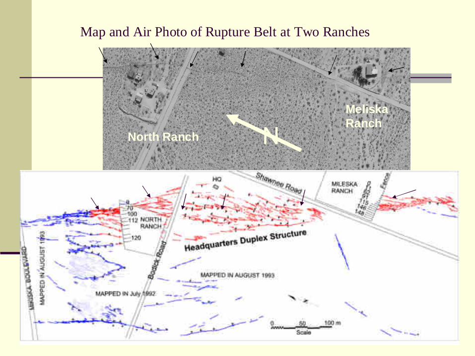
Map and Air Photo of Rupture Belt at Two Ranches
NNorth Ranch
MeliskaRanch
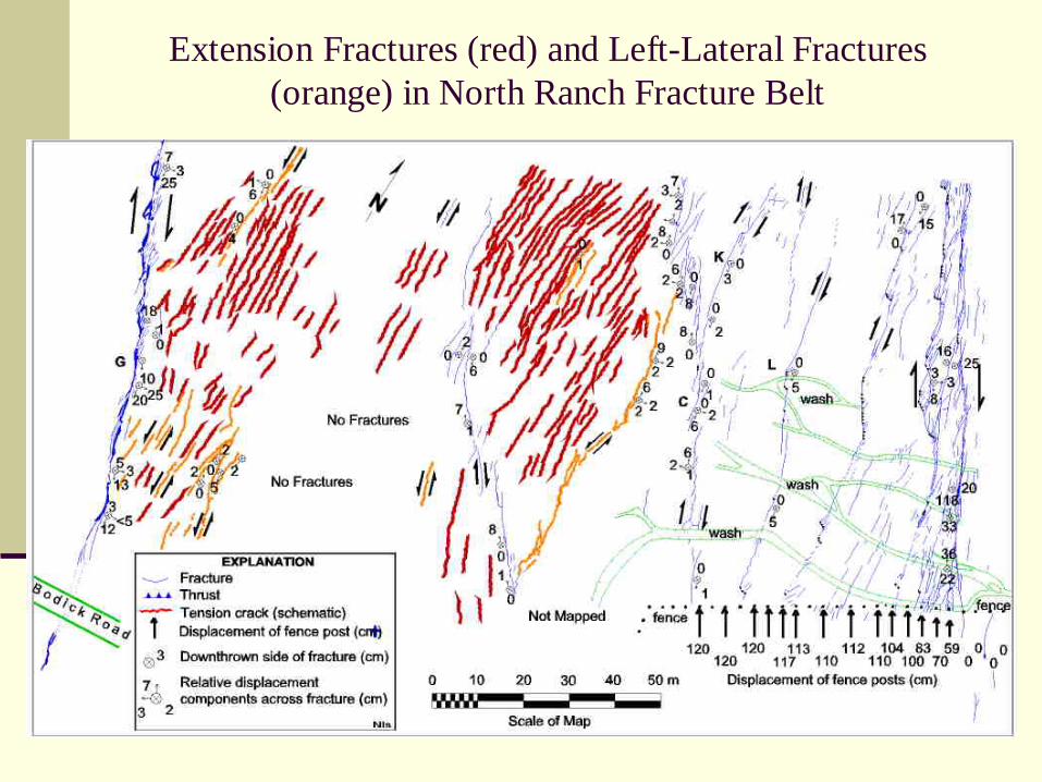
Extension Fractures (red) and Left-Lateral Fractures (orange) in North Ranch Fracture Belt
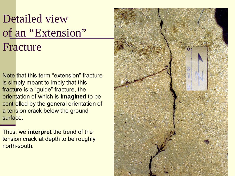
Detailed viewof an “Extension”Fracture
Note that this term “extension” fractureis simply meant to imply that thisfracture is a “guide” fracture, theorientation of which is imagined to becontrolled by the general orientation of a tension crack below the ground surface.
Thus, we interpret the trend of the tension crack at depth to be roughly north-south.
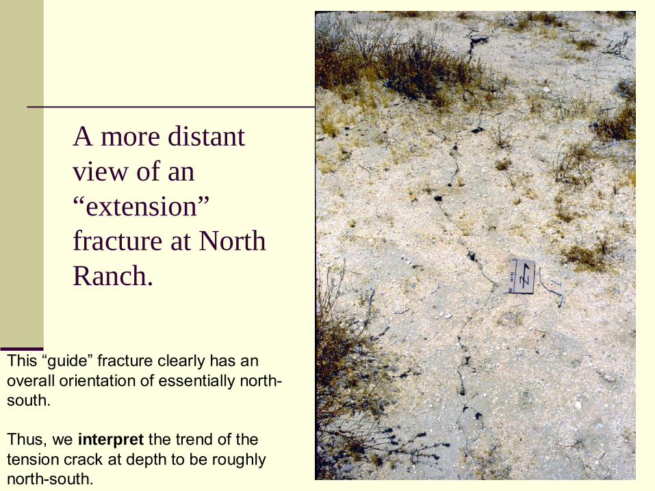
A more distant view of an“extension”fracture at NorthRanch.
This “guide” fracture clearly has an overall orientation of essentially north-south.
Thus, we interpret the trend of the tension crack at depth to be roughly north-south.
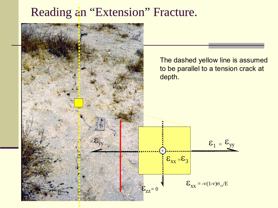
Reading an “Extension” Fracture.
εyy εyyε1
εxx = ε3
εxx = -ν(1-ν)σyy/Eεzz= 0
=
The dashed yellow line is assumed to be parallel to a tension crack atdepth.
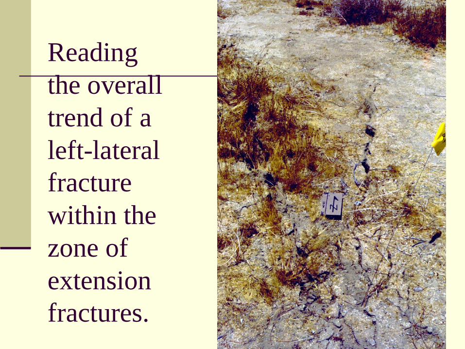
Reading the overall trend of a left-lateral fracture within the zone of extension fractures.
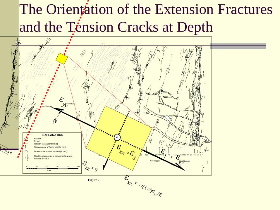
The Orientation of the Extension Fractures and the Tension Cracks at Depth
Figure 7
7
18
Not Mapped
fencefence
wash
wash
wash
slump
0
1
10
1510
2520
G
53
13
3
<512
73
25
0
20
5
0
2
0
2
0
4
01
6
0
20
6
1
7
0
8
1
0
0
1
9
22
6
22
73
24
328
20
62
20
8
0
28
0
0
3
0
10
62
62
1
0
1
0
5
0
5
17
0
15
0
16
25
20
118
33
3 3
8
36
22
120 120 120 120 117 113 110 112 110 104 100 83 70 59
Not Mapped Not Mapped
0 0
No FracturesNo Fractures
EXPLANATION
3
73
2
Scale
0 10 20 30 40 50m
Relat ive displacement components acrossfracture (in cm.)
Downthrown side of fracture (in cm.)
Displacement of fence post (in cm.)Tension crack (schemat ic)ThrustFracture
N
k R o a d
1
εyy
εyy
ε1
εxx = ε
3
εxx = -ν(1-ν)σ
yy/E
εzz = 0
=
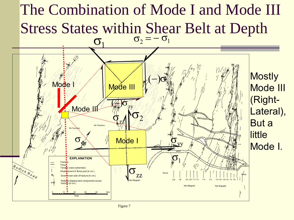
The Combination of Mode I and Mode III Stress States within Shear Belt at Depth
Figure 7
7
18
Not Mapped
fencefence
wash
wash
wash
slump
0
1
10
1510
2520
G
53
13
3
<512
73
25
0
20
5
0
2
0
2
0
4
01
6
0
20
6
1
7
0
8
1
0
0
1
9
22
6
22
73
24
328
20
62
20
8
0
28
0
0
3
0
10
62
62
1
0
1
0
5
0
5
17
0
15
0
16
25
20
118
33
3 3
8
36
22
120 120 120 120 117 113 110 112 110 104 100 83 70 59
Not Mapped Not Mapped
0 0
No FracturesNo Fractures
EXPLANATION
3
73
2
Scale
0 10 20 30 40 50m
Relative displacement components acrossfracture (in cm.)
Downthrown side of fracture (in cm.)
Displacement of fence post (in cm.)Tension crack (schematic)ThrustFracture
N
B o d i c k R o a d
1
(−)σyz
(−)σzy
σ1σ2 = − σ1
σ1
σ2
σyyσyy
σzz
σzz
Mode III
Mode IMostly Mode III (Right-Lateral),But a littleMode I.
Mode III
Mode I
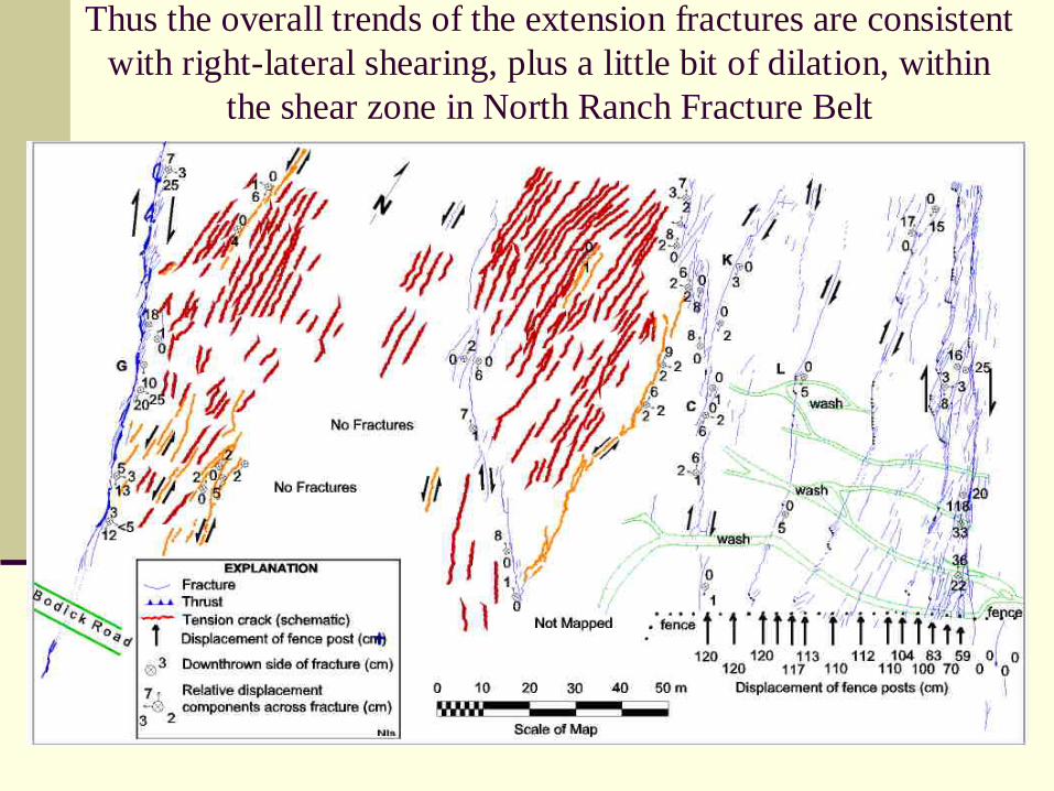
Thus the overall trends of the extension fractures are consistent with right-lateral shearing, plus a little bit of dilation, within
the shear zone in North Ranch Fracture Belt
Summary of Observations of Extension Fractures
These observations seem to indicate that:1). The irregular extension fractures have a definite overall trend at Two Ranches: N-S.2) They form a CW angle of about 30° with the walls of the fracture zone.3) The extension fractures and the presumed, underlying tension cracks indicate a wide belt of shearing, that is, a shear belt, much as we measured under the viaduct at Kaynaşlı.
TWO KINDS OF FRACTURING THAT WE OBSERVE:
MECHANICAL FRACTURINGA. Faults (Mode II or III failure)B. Cracks (or “Tension” cracks) (Mode I failure)
KINEMATIC (OR “GUIDE”) FRACTURINGA. “Extension” fractures: Guides to tension fractures at depth (?) Probably.B. Guide Fractures for probable faults at depth.
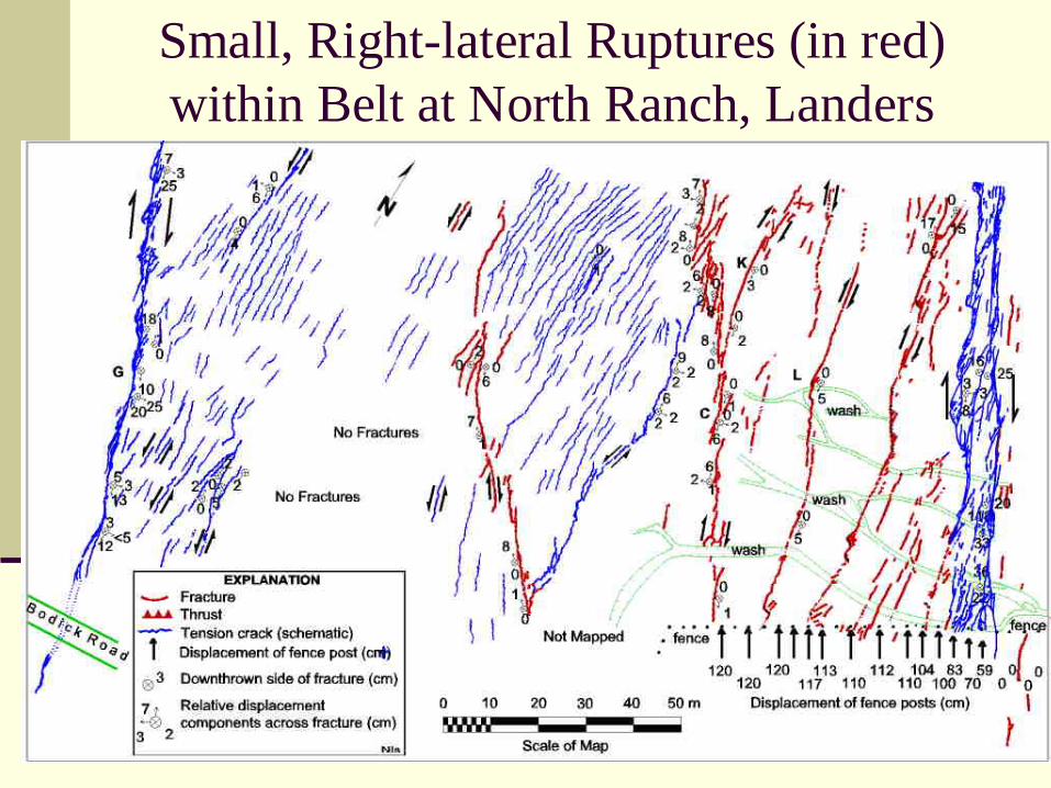
Small, Right-lateral Ruptures (in red) within Belt at North Ranch, Landers
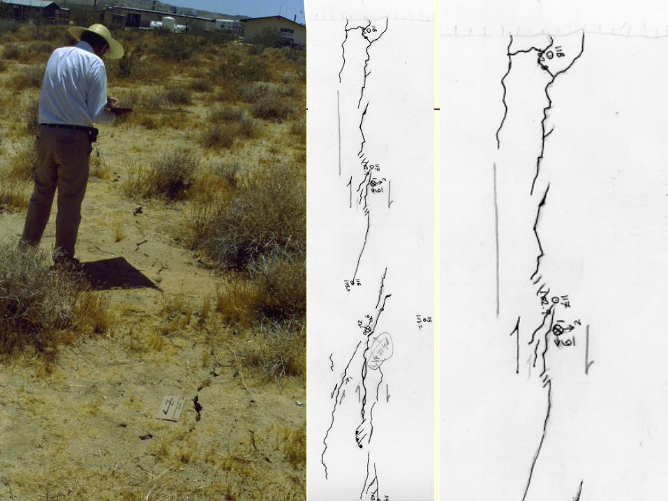
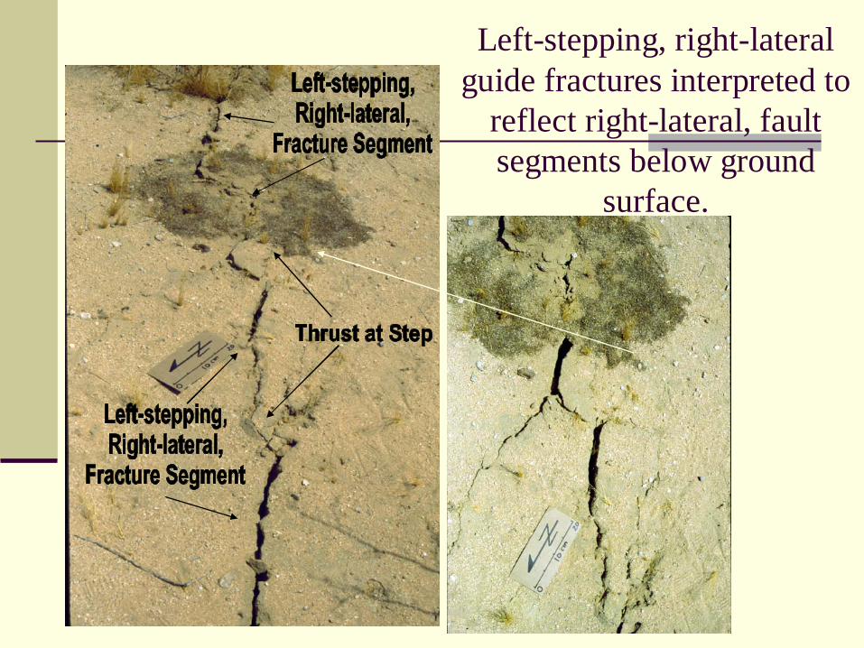
Left-stepping, right-lateral guide fractures interpreted to
reflect right-lateral, fault segments below ground
surface.
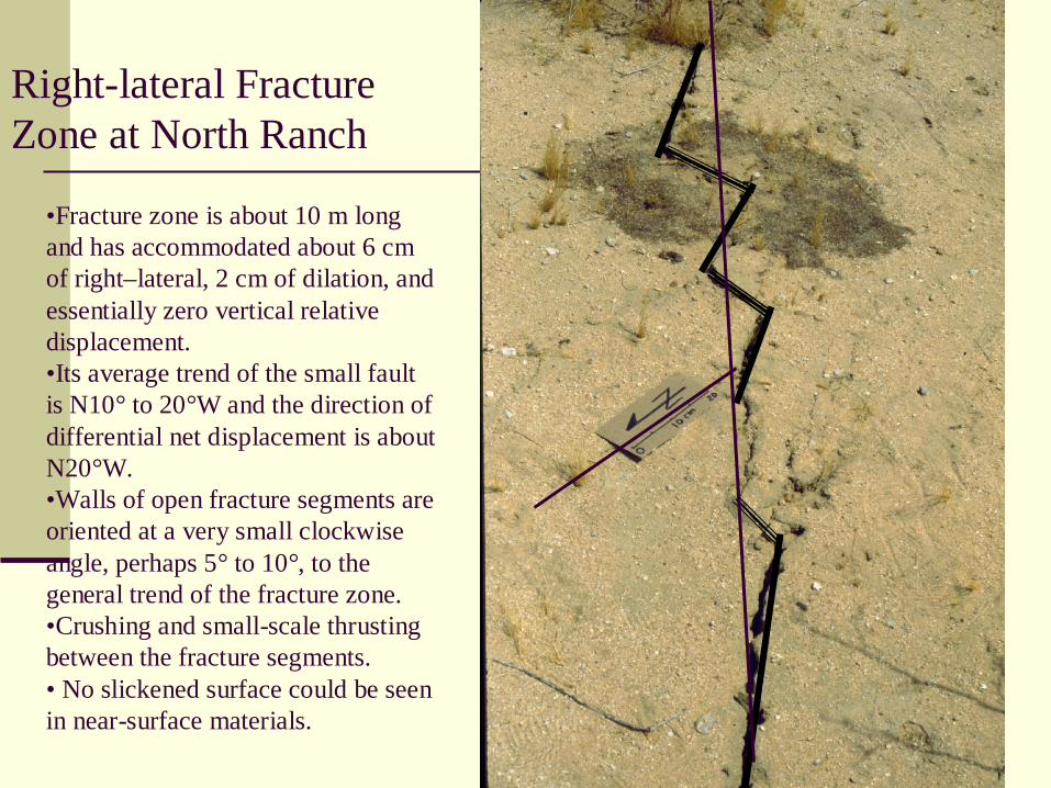
Right-lateral Fracture Zone at North Ranch
•Fracture zone is about 10 m long and has accommodated about 6 cm of right–lateral, 2 cm of dilation, and essentially zero vertical relative displacement.•Its average trend of the small fault is N10° to 20°W and the direction of differential net displacement is about N20°W.•Walls of open fracture segments are oriented at a very small clockwise angle, perhaps 5° to 10°, to the general trend of the fracture zone.•Crushing and small-scale thrusting between the fracture segments.• No slickened surface could be seen in near-surface materials.
THE END OF READING FRACTURES PART II: APPLICATION OF LINEAR FRACTURE MECHANICS