Embed Size (px)
Citation preview

Chapter 2Introduction to Continuum Mechanics
The mechanics of a deformable body treated here is based on Newton’s lawsof motion and the laws of thermodynamics. In this Chapter we present thefundamental concepts of continuum mechanics, and, for conciseness, the material ispresented in Cartesian tensor formulation with the implicit assumption of Einstein’ssummation convention. Where this convention is exempted we shall denote theindex thus: .Š˛/.
2.1 Newtonian Mechanics
Newtonian mechanics consists of
1. The first law (The law of inertia),2. The second law (The law of conservation of linear momentum), and3. The third law (The law of action and reaction).
Newton’s first law defines inertial frames of reference. In general it can bedescribed as follows; “if no force acts on a body, it remains immobilized or in astate of constant motion”. However, if this is true, the first law is obviously inducedby the second law,1 and the laws might be incomplete as a physical system. We mustrephrase the first law as follows:
The First Law: If no force acts on a body, there exist frames of reference, referredto as inertial frames, in which we can observe that the body is either stationary ormoves at a constant velocity.
1In the second law (2.2) if we set f D 0 and solve the differential equation, we obtain v D constantsince m D constant, which suggests that the first law is included in the second law. This apparentcontradiction results from the misinterpretation of the first law.
Y. Ichikawa and A.P.S. Selvadurai, Transport Phenomena in Porous Media,DOI 10.1007/978-3-642-25333-1 2, © Springer-Verlag Berlin Heidelberg 2012
9

10 2 Introduction to Continuum Mechanics
We now understand that the first law assures the existence of inertial frames, andthe second and third laws are valid in the inertial frames. This is the essence ofNewtonian mechanics.
Let m and v be the mass and velocity of a body, respectively, then the momentump is given by
p D mv: (2.1)
We now have the following:
The Second Law: In an inertial frame, if a force f acts on a body, the followinglaw of conservation of linear momentum is valid:
dpdt
D d.mv/
dtD f (2.2)
Since the mass m is conserved in Newtonian mechanics, (2.2) can be rewritten as
mdvdt
D f : (2.3)
Let us consider a material point which is represented by two different frames as.x; t/ and .x�; t�/ where x; x� denote positions and t; t� denote time. Under theGalilean transformation given by
x� D Qx C V t; t� D t C a; (2.4)
both frames form the equivalent inertial frames (Fig. 2.1). This is referred to as theGalilean principle of relativity. Here Q is a time-independent transformation tensor(cf. Appendix A.3), V is a constant vector and a is a scalar constant.
The Galilean transformation (2.4) gives, in fact, the condition which results inthe law of conservation of linear momentum (2.2) in both the frames .x; t/ and.x�; t�/. That is, differentiating (2.4) yields
v� D dx�
dt�D Q
dx
dtC V D Qv C V
Fig. 2.1 Galileantransformation

2.2 Deformation Kinematics 11
and the force vector f is transformed in the same manner:
f � D Q f : (2.5)
The mass conservation law is m� Dm, and (2.5) suggests that the law of conserva-tion of linear momentum is satisfied in the inertial frames in the following manner:
f � D m� dv�
dt�D m
d.Q v C V /
dtD Q
�m
dvdt
�D Q f : (2.6)
Note that the force vector represented in the form of (2.5) is a fundamentalhypothesis of Newtonian mechanics (i.e., the frame indifference of a force vector;see Sect. 2.2.2). The third law gives the interacting forces for a two-body problem,and this will not be treated here.
Note 2.1 (Inertial frame and the relativity principle). The first law (i.e., the law ofinertia) gives a condition that there are multiple frames of equivalent inertia thatare moving under a relative velocity V . Therefore, the first law guarantees that thesecond law (i.e., the law of conservation of linear momentum) is realized in anyinertial frame. This implies that the second law is not always appropriate in differentframes of reference, which are moving under a general relative velocity. In fact, inan accelerated frame that includes rotational motion, such as on the surface of Earth,there is a centrifugal force and a Coriolis effect. In Sect. 2.2.2 we will treat a generallaw of change of frame, which is related to a constitutive theory that describes thematerial response (see Sect. 2.8).
If the relative velocity V of the Galilean transformation (2.4) approaches thespeed of light c, the uniformity of time is not applicable, and the Newtonianframework is no longer valid. That is, the Galilean transformation is changedinto the Lorentz transformation under invariance of Maxwell’s electromagneticequations, and the equation of motion is now described in relation to Einstein’stheory of relativity. �
2.2 Deformation Kinematics
When we consider the motion of a material body, constituent atoms and moleculesare not directly taken into consideration since this will require an inordinate amountof analysis. Therefore we represent the real material by an equivalent shape of asubdomain of the n-dimensional real number space R
n, and apply the Newtonianprinciples to this image. This procedure leads to Continuum Mechanics; the term‘continuum’ is a result of the continuity properties of the n-dimensional real numberspace Rn.

12 2 Introduction to Continuum Mechanics
2.2.1 Motion and Configuration
Consider a material point X in the body B, and we have an image in then-dimensional real number space Rn that is referred as a configuration.2 We choosethe configuration, X.X/ 2 �0 � R
n, at the time t D t0 as a reference configuration,and treat the subsequent deformation and motion of the current configuration,x 2 � � R
n, at the time t D t with respect to the reference configuration (Fig. 2.2).Assume that a reference point X 2 �0 moves to the current point x 2 �. The
motion is represented asx D x.X ; t/ (2.7)
Note that the time change x.X ; t/ of a specific point X gives a trajectory. Then thevelocity of the material point is calculated by
v.X ; t/ D dx
dt.X ; t/ (2.8)
Fig. 2.2 Motion and deformation of a material body
2‘Configuration’ is defined as an invertible continuous function that maps every material pointX 2 B to a point z in a subset of the n-dimensional real number space R
n. A time-dependentmotion is considered; therefore the configuration is a function of the material point X andtime t . The configuration at a given time t0 is set as a reference configuration �, and thepoint X 2 R
n corresponding to a material point X is written as X D �.X/; X D ��1.X /
where ��1 is an inverse mapping of �. The current configuration � at time t maps X tox 2 R
n as x D �.X; t/; X D ��1.X; t /. The composite function �� D � ı ��1 is introduced asx D �.��1.X /; t / D �� D � ı ��1.X; t / D ��.X; t /. The function �� gives a mapping betweenthe position vector X in the reference configuration and the position vector x in the currentconfiguration. Since this formal procedure is complicated, the above simplified descriptions areemployed.

2.2 Deformation Kinematics 13
We should pay attention to the fact that the velocity v has a simple differential formof (2.8) with respect to t , since x.X ; t/ is a function both of X and of t but X is afixed frame of reference.
Two material points can never occupy the same position, therefore (2.7) has aunique inverse:
X D X.x; t/ (2.9)
This relation permits the definition of the velocity v.X ; t/; this can be written as afunction of x and t :
v.X.x; t/; t/ D v.x; t/: (2.10)
We can generalize this procedure: If a function � is represented in terms of.X ; t/, we call it the Lagrangian description, and if � is given in terms of .x; t/, it isthe Eulerian description. The choice of the form is arbitrary but will be influencedby any advantage of a problem formulation in either description. For example,in solid mechanics, the Lagrangian description is commonly used, while in fluidmechanics the Eulerian description is popular. This is because in solid mechanicswe can attach labels (e.g., visualize ‘strain gauges’ at various points) on the surfaceof a solid body, and each material point can be easily traced from the referencestate to the current state. On the other hand for a fluid we measure the velocityv or pressure p at the current position x, therefore the Eulerian description betterrepresents the fluid (note that for a fluid it is difficult to know the exact referencepoint X corresponding to all the current points x).
The coordinate system with the basis fEI g .I D1; 2; 3/ for the undeformed body�0 is usually different from the coordinate system with the basis feig .i D1; 2; 3/
that describes the deformed body � in the current configuration (Fig. 2.2):
X D XI EI ; x D xi ei : (2.11)
fEI g; fei g represent the orthogonal coordinate systems (i.e., Cartesian); we willemploy the same orthogonal coordinate systems fEI gDfei g for simplicity unlessotherwise mentioned. Then, the position vectors X and x can be written as
X D Xiei ; x D xi ei
Let �.X ; t/ be a Lagrangian function. Since X is time-independent, the timedifferentiation P� is simply given by
P�.X ; t/ D d�
dt: (2.12)
Here P� D d�=dt is referred to as the material time derivative of �.X ; t/. On theother hand, for an Eulerian function �.x; t/ the total differential d�.x; t/ can bewritten as
d�.x; t/ D @�
@tdt C @�
@xi
dxi ;

14 2 Introduction to Continuum Mechanics
and vi Ddxi =dt , and therefore we have the following relationship between thematerial time derivative and Eulerian time derivative
d�
dtD @�
@tC v � r�: (2.13)
Here the symbol r (called ‘nabla’) implies3
r D ei
@
@xi
: (2.14)
The second term of the r.h.s. of (2.13) gives a convective term.The velocity v is written either in the Lagrangian form or in the Eulerian form;
therefore the acceleration a can be represented in either form:
a.X; t/ D dvdt
D @v@t
C v � rv D a.x; t/ (2.15)
In indicial notation (2.15) is given by
ai D dvi
dtD @vi
@tC vj
@vi
@vj
: (2.16)
Note 2.2 (Differentiation of vector and tensor valued functions). Let uDuiei andT DTijei ˝ ej be vector and tensor valued functions. It is understood that thegradients grad u; grad T can be of two forms:
grad u D
8ˆ<ˆ:
u ˝ r D @ui
@xj
ei ˝ ej ;
r ˝ u D @ui
@xj
ej ˝ ei ;
grad T D
8ˆ<ˆ:
T ˝ r D @Tij
@xk
ei ˝ ej ˝ ek;
r ˝ T D @Tjk
@xi
ei ˝ ej ˝ ek:
The former are called the right form, and the latter are the left form.
3If the gradient is used with respect to Eulerian coordinates with the basis fei g, it is denoted as(2.14). If we explicitly explain the gradient with respect to the Eulerian system, it is denoted as
grad D r x D ei
@
@xi
:
If the gradient is operated with respect to Lagrangian coordinates fEI g, it is represented as
Grad D r X D EI
@
@XI
:

2.2 Deformation Kinematics 15
Right and left forms of divergence div u; div T and rotation rot u; rot T aregiven by
div u D
8<ˆ:
u � r D @ui
@xi
;
r � u D @ui
@xi
;
div T D
8<ˆ:
T � r D @Tij
@xj
ei ;
r � T D @Tji
@xj
ei ;
rot u D
8ˆ<ˆ:
u ^ r D eijk@ui
@xj
ek;
r ^ u D ejik@ui
@xj
ek;
rot T D
8ˆ<ˆ:
T ^ r D ejkl@Tik
@xl
EI ˝ ej ;
r ^ T D eikl@Tlj
@xk
EI ˝ ej ;
In this volume we will predominantly use the right form, and we symbolically writethe right forms in the same manner as the left form: e.g.
grad u D @ui
@xj
ei ˝ ej ; grad T D @Tij
@xk
ei ˝ ej ˝ ek;
div u D @ui
@xi
; div T D @Tij
@xj
ei ;
rot u D eijk@ui
@xj
ek; rot T D ejkl@Tik
@xl
ei ˝ ej
In addition, if the right-divergence form of the second-order tensor T DTijei ˝ ej
is as given above, the divergence theorem (B.6) given in Appendix B.2 can bewritten as Z
G
div T dv DZ
G
r � T dv DZ
@G
T n ds:
If u and T are given as functions of the reference basis such thatuDuI .X/EI ; T DTIJ.X/EI ˝ EJ , we have
Grad u D @uI
@XJ
EI ˝ EJ ; Grad T D @TIJ
@XK
EI ˝ EJ ˝ EK;
Div u D @uI
@XI
; Div T D @TIJ
@XJ
EI ;
Rot u D eIJK@uI
@XJ
EK; Rot T D eJKL@TIK
@XL
EI ˝ EJ : �

16 2 Introduction to Continuum Mechanics
2.2.2 Changes of Frame and Frame Indifference |
Let us consider two different points x and x0 in the current body, and introducea two-point vector uDx �x0 (u does not imply displacement). Then, it is easilyobserved that the length j u jD .u � u/1=2 is an invariant; i.e., it has the same valuein any coordinate system. We call this property of j u j the principle of frameindifference. The concept of frame indifference is a fundamental requirement fora constitutive theory between, for example, stress and strain (see Sect. 2.8).
The frame indifference of the two-point vector u is proved as follows: Let usintroduce two coordinate systems, System 1 and System 2, which have bases fei gand fe�
i g, respectively (Fig. 2.3). In the framework of Newtonian mechanics, thetwo-point vector x�x0 and time t of System 1 can be related to x� �x�
0 and t� ofSystem 2 by
x� � x�0 D Q.x � x0/ (2.17)
t� D t � a (2.18)
where QDQije�i ˝ ej is the following coordinate transformation tensor:
e�i D Qei : (2.19)
The tensor Q is orthonormal:
Q QT D I�; QT Q D I (2.20)
where I is the unit tensor defined on System 1, and I� is that defined on System 2.Note that a in (2.18) is a constant.4 It is understood that the length jx�x0j is invariantunder the change of frame since from (2.17) to (2.20) we have
jx� � x�0 j2 D .x � x0/ � QT Q.x � x0/ D jx � x0j2: (2.21)
In general, a frame indifferent scalar function f is defined by
f �.x�/ D f .x/: (2.22)
The frame indifferent vector function u is given by
u�.x�/ D Q u.x/; u.x/ D QT u�.x�/: (2.23)
4Here we deal with a general case in which two coordinate systems may not be inertial systems. Ifboth are inertial systems, Q is time-independent as given by (2.4). Therefore, we have
x� D Q x C V t; x�
0 D Q x0 C V t ) u D x� � x�
0 D Q.x � x0/;
which shows that the two-point vector u is frame indifferent.

2.2 Deformation Kinematics 17
Fig. 2.3 Coordinatetransformation and frameindifferent vector
A frame indifferent second-order tensor function T is characterized by theframe indifference of a transformed vector v D T u. That is, let u be a frameindifferent vector (u� D Q u), and v and v� be the vectors corresponding to u andu� transformed by T and T � such that
v D T u; v� D T � u�:
Then, if v� D Q v, T is said to be frame indifferent. Now we have
v� D Q� v D T � u� D T � Q u ) v D QT T � Q u:
Therefore the requirement for frame indifference of a second-order tensor T isdefined by
T D QT T � Q; T � D Q T QT : (2.24)
2.2.3 Motion in a Non-inertial System |
We consider an equation of motion for the case where System 1 is inertial while Sys-tem 2 is non-inertial. Since the two-point vector x�x0 should be frame indifferent,satisfying (2.17) and (2.18), a position vector x�.t/ in System 2 is given by
x�.t/ D x�0 .t/ C Q.t/.x � x0/ (2.25)
where we can regard x0 as the origin of the coordinate system O , and x�0 .t/ as the
origin of the coordinate system O� (see Fig. 2.3). Taking a material time derivativeof (2.25) and substituting the inverse relation of (2.17) gives the velocity:
v� D dx�0
dtC �.x� � x�
0 / C Qv; (2.26)
� D dQ
dtQT (2.27)

18 2 Introduction to Continuum Mechanics
The result (2.26) shows that the velocity vector v is not frame indifferent. Notethat by differentiating (2.20)1 the second-order tensor � is understood to be anti-symmetric:
dQ
dtQT C Q
dQT
dtD 0 ) � D dQ
dtQT D �Q
dQT
dtD ��T : (2.28)
The acceleration vector is given by a material time derivative of (2.26):
a� D dv�
dtD d 2x�
0
dt2C 2�
�v� � dx�
0
dt
�C
�d�
dt� �2
�.x� � x�
0 / C Qdvdt
(2.29)
This suggests that the acceleration is not frame indifferent.Now we define a rotation vector ! with respect to the original coordinate
system by
!i D �1
2eijk�kj D 1
2eijk�jk (2.30)
then for any vector a we have�a D ! ^ a (2.31)
Thus, (2.29) can be written as
dv�
dtD d 2x�
0
dt2C d�
dtQ.x�x0/C!^Œ! ^ Q.x � x0/�C2!^QvCQ
dvdt
(2.32)
The third term of the r.h.s. of this equation gives a centrifugal force and the fourthis the Coriolis force.
As shown by (2.5), a fundamental hypothesis of Newtonian mechanics is that theforce f is frame indifferent (f � DQ f ). Therefore, referring to (2.32) and (2.27),the equation of motion in System 2, which is non-inertial, can be written as
m� dv�
dt� D f � C f ai; (2.33)
f ai D m
�d 2x�
0
dt2C d�
dt.x� � x�
0 / C ! ^ ! ^ .x� � x�0 /
C2! ^�
v� � dx�0
dt� �.x� � x�
0 /
��(2.34)
where f ai is an apparent inertial force observed in the non-inertial system.

2.2 Deformation Kinematics 19
2.2.4 Deformation Gradient, Strain and Strain Rate
We distinguish between the coordinate system fEI g of the Lagrangian descriptionand the coordinate system fei g of the Eulerian description in order to understand therelationship between both systems.
As shown in Fig. 2.2, an increment vector dx Ddxi ei of a point x 2 � in thedeformed body � is related to the increment dX DdXI EI of the correspondingpoint X 2�0 in the undeformed body �0 by
dx D F dX (2.35)
where the second-order tensor F is the deformation gradient;
F D Grad x D rX x D FiI ei ˝ EI ; (2.36)
FiI D @xi
@XI
; Grad D rX D EI
@
@XI
(2.37)
which relates the infinitesimal line segment dX 2�0 to the corresponding segmentdx 2 �. As observed in (2.36), the deformation gradient F plays a role in thecoordinate transformation from EI to ei . Since no material point vanishes, there isan inverse relation of F :
F �1 D grad X D r xX D F �1I i EI ˝ ei ; (2.38)
F �1I i D @XI
@xi
; grad D r x D ei
@
@xi
: (2.39)
If the right form (see Note 2.2) is employed, the related forms of deformationgradient can be written as follows:
F D @xi
@XI
ei ˝ EI ; F T D @xi
@XI
EI ˝ ei ; (2.40)
F �1 D @XI
@xi
EI ˝ ei ; F �T D @XI
@xi
ei ˝ EI : (2.41)
Here F �T implies .F �1/T .Now we need to measure the extent of deformation of an elemental length located
at a material point. To do so, we compare the length jdxj with its original length jdXj(see Fig. 2.2) by comparing the difference of both lengths as a squared measure:
j dx j2 � j dX j2 D dx � dx � dX � dX
Substituting the deformation gradient yields
dx � dx D dX � C dX ; dX � dX D dx � B�1dx

20 2 Introduction to Continuum Mechanics
where
C D F T F D FkI FkJ EI ˝ EJ ; B D F F T D FiI FjI ei ˝ ej (2.42)
C is referred to as the right Cauchy-Green tensor and B the left Cauchy-Greentensor. Then the deformation measure can be written as
j dx j2 � j dX j2 D dX � 2E dX D dx � 2e dx (2.43)
where we set
E D 1
2.C � I/ D 1
2.CIJ � ıIJ/ EI ˝ EJ ; (2.44)
e D 1
2
�i � B�1
� D 1
2
�ıij � B�1
ij
�ei ˝ ej (2.45)
Note that I DıIJ EI ˝ EJ and i Dıij ei ˝ ej are the unit tensors in the referenceand current configurations, respectively. E is referred to as the Lagrangian strain orGreen strain, and e the Eulerian strain or Almansi strain (see, e.g., Malvern 1969;Spencer 2004).
Since the deformation gradient F is invertible and positive definite (det F > 0),we can introduce the following polar decomposition:
F D RU D VR (2.46)
where
R D RiI ei ˝ EI ; U D UIJ EI ˝ EJ ; V D Vij ei ˝ ej (2.47)
R is referred to as the rotation tensor, U the right stretch tensor, V the left stretchtensor. R is orthonormal (RT R DI ; RRT D i ), which gives the rotation of C andB�1 to their principal axes. Under the polar decomposition we have
C D U 2; B D V 2 (2.48)
As understood from (2.48), U and V are symmetric and positive definite.
Note 2.3 (Small strain theory). In most textbooks on elasticity theory a displace-ment vector is defined as uDx �X . However we know that x Dxi ei , X DXI EI
and the transformation of both bases are locally defined by the deformation gradientF ; therefore it is difficult to introduce the globally defined displacement vector uunless a common rectangular Cartesian coordinate system is used.
Now let us use a common basis ei and introduce an incremental form as
du D dx � dX D .F � i / dX D H dX (2.49)

2.2 Deformation Kinematics 21
where
H D @u@X
D F � i D .Fij � ıij/ ei ˝ ej (2.50)
Then the Green strain is given by
E D 1
2
�H C H T C H T H
� D 1
2
�@ui
@Xj
C @uj
@Xi
C @uk
@Xi
@uk
@Xj
�ei ˝ ej (2.51)
Since the third term of the r.h.s. is second-order infinitesimal, the small straintensor is given by
"ij D 1
2
�@ui
@xj
C @uj
@xi
�(2.52)
where we identify the coordinates Xi with xi (Little 1973; Davis and Selvadurai1996; Barber 2002).
The strain with components given by (2.52) is referred to as the tensorial strain,while the strain in which the shearing components are changed into
�yz D @uy
@zC @uz
@y; �zx D @uz
@xC @ux
@z; �xy D @ux
@yC @uy
@x
which can be denoted by the vector
" D �"xx; "yy; "zz; �xy; �yz; �zx
T(2.53)
that is referred to as the engineering strain. �
Note 2.4 (Generalized strain measure (Hill 1978)|). Since the right Cauchy-Greentensor C DF T F is symmetric and the components are real numbers, there are threereal eigenvalues that are set as �2
i .i D 1; 2; 3/ and the corresponding eigenvectorsare given by N i ; then we have
�F T F
�N i � �2
i N i D 0; N i � N j D ıij .i W not summed/: (2.54)
Let us set a material fiber along N i as dX i , therefore we can write
dX i D dXi N i ) �F T F
�dX i D �2
i dX i .i W not summed/
(2.55)
where �i is referred to as the principal stretch , and N i .i D1; 2; 3/ form Lagrangiantriads. Referring (2.48)1, the right stretch tensor U can be written as
U D Pi
�i N i ˝ N i : (2.56)

22 2 Introduction to Continuum Mechanics
The rotation tensor R given by (2.47)1 transforms the Lagrangian triads N i into theEulerian triads ni :
ni D R N i ; R D Pi
ni ˝ N i : (2.57)
The left stretch tensor V given by (2.47)3 can now be written as
V D Pi
�i ni ˝ ni : (2.58)
Following Hill (1978) the generalized Lagrangian strain measure is defined by
E D Pi
f .�i / N i ˝ N i : (2.59)
Here f .�i / is a scale function which satisfies the conditions
f .1/ D 0; f 0.1/ D 1:
Consider the following example:
f .z/ D z2n � 1
2n: (2.60)
We can introduce the following family of n-th order Lagrangian strain measures:
E .n/ DX
i
.�i /2n � 1
2nN i ˝ N i : (2.61)
The Green strain given by (2.44) corresponds to E .1/. Furthermore from (2.60) wehave
limn!0
.�i /2n � 1
2nD ln �i :
As n!0, the logarithmic strain E.0/ is given by
E.0/ D ln U D Pi
ln.�i / N i ˝ N i : (2.62)
The generalized Eulerian strain measure is given by
e D Pi
f .�i / ni ˝ ni D R ERT ; (2.63)
and the family of n-th order Eulerian strain measures is introduced by

2.2 Deformation Kinematics 23
e.n/ DX
i
.�i /2n � 1
2nni ˝ ni ; e.0/ D ln V D P
i
ln.�i / ni ˝ ni : (2.64)
It should be noted that E.�1/ ¤ e.1/. �
Recall the definition of the deformation gradient dx DF dX ; its material time-derivative defines the following velocity gradient:
Pdx D PF dX D Ldx ) L � PF F �1: (2.65)
Since the direct forms of PF ; F �1 are given by
PF D PFiI ei ˝ EI D @vi
@XI
ei ˝ EI ; F �1 D @XI
@xi
EI ˝ ei (2.66)
L can be written as
L D grad v D @vi
@xk
ei ˝ ek (2.67)
On the other hand, F F �1 Di , therefore taking its material time differential with(2.65) PF DLF yields the inverse of PF :
PF �1 D �F �1L: (2.68)
The velocity gradient L is decomposed into its symmetric part D, called thestretch tensor or rate-of-deformation tensor, and its anti-symmetric part W , calledthe spin tensor:
L D PF F �1 D D C W ; (2.69)
D D 1
2
�L C LT
�; W D 1
2
�L � LT
�: (2.70)
The material time differentiation of the Green strain E given by (2.44) is
PE D 1
2
PF TF C F T PF
�D F T DF ) D D F �T PEF �1 (2.71)
where (2.65) is used.
Note 2.5 (Embedded coordinates |). In solids we can trace each material point X
by attaching labels on its surface during deformation. Then, as shown in Fig. 2.4, it iseasy to introduce a coordinate system in which the label values of the coordinates arenot changed (xi DXi ) but the reference basis G i (before deformation) is changedinto the current basis g i (after deformation). This is referred to as the embeddedcoordinate system.

24 2 Introduction to Continuum Mechanics
Fig. 2.4 Embedded coordinate system
In the embedded coordinate system, the transformation rule of the base vectorsis given by
gi .t/ D F .t/G i ) F .t/ D g i .t/ ˝ G i ; (2.72)
and the following relationships are obtained:
F �1 D G i ˝ gi ; G i D F �1gi ; (2.73)
F �T D gi ˝ G i ; gi D F �T G i : (2.74)
The unit tensor in the current deformed body is written as i Dıji g i ˝
gj Dıij gi ˝ gj Dgij g i ˝ gj Dgij gi ˝ gj , and the right Cauchy-Green tensor C
is given by
C D F T F D .G i ˝ gi /.gj ˝ G j / D gij G i ˝ G j : (2.75)
Let an arbitrary second-order tensor K in the current body be written as
K D K ijgi ˝ gj D Kij g i ˝ gj D K
ji g i ˝ gj D Kij gi ˝ gj ; (2.76)
then the second-order tensors that have the same components in the undeformedbody are given by
K .I / D K ij G i ˝ G j D F �1KF �T
K .II/ D Kij G i ˝ G j D F �1KF
K .III/ D Kji G i ˝ G j D F T KF �T
K .IV/ D Kij G i ˝ G j D F T KF :
(2.77)
2.2 Deformation Kinematics 25
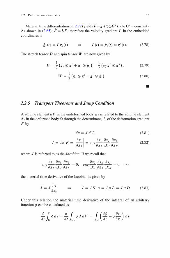
Material time differentiation of (2.72) yields PF D Pgi .t/˝G i (note G iD constant).As shown in (2.65), PF DLF , therefore the velocity gradient L in the embeddedcoordinates is
Pg i .t/ D Lgi .t/ ) L.t/ D Pgi .t/ ˝ gi .t/: (2.78)
The stretch tensor D and spin tensor W are now given by
D D 1
2
� Pgi ˝ gi C g i ˝ Pgi
� D 1
2
� Pgij gi ˝ gj�
; (2.79)
W D 1
2
� Pg i ˝ gi � gi ˝ Pg i
�(2.80)
�
2.2.5 Transport Theorems and Jump Condition
A volume element dV in the undeformed body �0 is related to the volume elementdv in the deformed body � through the determinant, J , of the deformation gradientF by
dv D J dV; (2.81)
J D det F Dˇˇ @xi
@XI
ˇˇ D eIJK
@x1
@XI
@x2
@XJ
@x3
@XK
(2.82)
where J is referred to as the Jacobian. If we recall that
eIJK@x1
@XI
@x1
@XJ
@x2
@XK
D 0; eIJK@x2
@XI
@x2
@XJ
@x3
@XK
D 0; � � �
the material time derivative of the Jacobian is given by
PJ D J@vk
@xk
) PJ D J r � v D J tr L D J tr D (2.83)
Under this relation the material time derivative of the integral of an arbitraryfunction � can be calculated as
d
dt
Z�
� dv D d
dt
Z�0
� J dV DZ
�
�d�
dtC �
@vi
@xi
�dv

26 2 Introduction to Continuum Mechanics
We now have the following Reynolds’ transport theorem:
d
dt
Z�
� dv DZ
�
�d�
dtC �r � v
�dv D
Z�
�d�
dtC � tr L
�dv
DZ
�
�@�
@tC r � .�v/
�dv D
Z�
@�
@tdv C
Z@�
�v � n ds: (2.84)
Next we give the transport theorem for a surface integral: The determinant of a.3 � 3/-matrix A is given by
erst det A D eijkAirAjsAkt:
Therefore (2.81) can be written as
eijk J �1 D eIJK
@XI
@xi
@XJ
@xj
@XK
@xk
; eIJK J D eijk@xi
@XI
@xj
@XJ
@xk
@XK
A surface element dS DdX ^ ıX consists of line elements dX and ıX in theundeformed body and the corresponding surface element dsDdx ^ ıx consists ofline elements dx and ıx in the deformed body
dS D N dS D dX ^ ıX ; ds D n ds D dx ^ ıx (2.85)
where N and n are outward normals of dS and ds, respectively (Fig. 2.5). If dS isdeformed into ds, (2.85)1 implies
NI dS D eIJK dXJ dXK D eIJK@XJ
@xj
@XK
@xk
dxj dxk;
and we have
@XI
@xi
NI dS D eIJK@XI
@xi
@XJ
@xj
@XK
@xk
dxj dxk D J �1ni ds ) ni ds D J@XI
@xi
NI dS
Fig. 2.5 Surface elements inthe reference body C0 and thecurrent body C
2.2 Deformation Kinematics 27
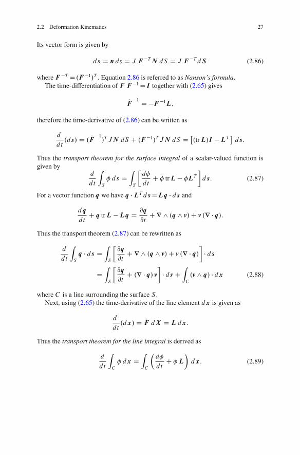
Its vector form is given by
ds D n ds D J F �T N dS D J F �T dS (2.86)
where F �T D .F �1/T . Equation 2.86 is referred to as Nanson’s formula.The time-differentiation of F F �1 DI together with (2.65) gives
PF �1 D �F �1L;
therefore the time-derivative of (2.86) can be written as
d
dt.ds/ D . PF �1
/T J N dS C .F �1/T PJ N dS D �.tr L/I � LT
ds:
Thus the transport theorem for the surface integral of a scalar-valued function isgiven by
d
dt
ZS
� ds DZ
S
�d�
dtC � tr L � �LT
�ds: (2.87)
For a vector function q we have q � LT dsDLq � ds and
dq
dtC q tr L � Lq D @q
@tC r ^ .q ^ v/ C v .r � q/:
Thus the transport theorem (2.87) can be rewritten as
d
dt
ZS
q � ds DZ
S
�@q
@tC r ^ .q ^ v/ C v .r � q/
�� ds
DZ
S
�@q
@tC .r � q/ v
�� ds C
ZC
.v ^ q/ � dx (2.88)
where C is a line surrounding the surface S .Next, using (2.65) the time-derivative of the line element dx is given as
d
dt.dx/ D PF dX D L dx:
Thus the transport theorem for the line integral is derived as
d
dt
ZC
� dx DZ
C
�d�
dtC � L
�dx: (2.89)

28 2 Introduction to Continuum Mechanics
For a vector function q this can be written as
d
dt
ZC
q � dx DZ
C
�dq
dtC LT q
�� dx: (2.90)
We next consider transport theorems involving a singular surface † that separatesa body � into �C and �� (Fig. 2.6). For example, a singular surface correspondsto the front of a shock wave causing a sonic boom or a migrating frozen front duringground freezing. Let the velocity of the singular surface † be V , @�C be the surfaceof �C except for †, @�� be the surface of �� except for †, and n be a unit normalon † directed to �C.
Let � be any function. �C implies the value of � on † approached from �C, and,similarly, �� is the value approached from ��. By applying the transport theorem(2.84) at each domain we have
d
dt
Z�C
� dv DZ
�C
@�
@tdv C
Z@�C
�v � n ds �Z
†
�CV � n ds
d
dt
Z��
� dv DZ
��
@�
@tdv C
Z@��
�v � n ds CZ
†
��V � n ds
where v is the velocity of each material point. Adding both equations underVn DV �n yields the following Reynolds’ transport theorem with a singular surface:
d
dt
Z�
� dv DZ
�
@�
@tdv C
Z@�
�v � n ds �Z
†
ŒŒ���Vn ds (2.91)
whereŒŒ��� D �C � �� (2.92)
implies a jump of the function � on †.We will show in Sects. 2.3–2.5 that physical conservation laws can be written in
the following form:
Fig. 2.6 Singular surface

2.3 Mass Conservation Law 29
Fig. 2.7 Infinitesimaldomain involving a singularsurface
d
dt
Z�
' dv DZ
�
s dv CZ
@�
q ds (2.93)
where s is a source per mass of the field variable ' and q is a flux flowing intothe body � through the surface @�. We then apply the transport theorem (2.91) foran infinitesimal domain with its boundary @ (Fig. 2.7) using the conservationlaw (2.93):
Z
@.'/
@tdv C
Z@
' v � n ds �Z
†
ŒŒ'��Vn ds DZ
s dv CZ
@
q ds:
If the thickness ı of the domain approaches zero, all the volumetric terms vanish:
Z†
ŒŒ' .V � v/ � n C q�� ds D 0:
We can conclude that, for the conservation law (2.93) involving the singular surface†, we have the following singular surface equation:
ŒŒ' .V � v/ � n C q�� D 0: (2.94)
2.3 Mass Conservation Law
We refer again to Fig. 2.2. If there is no mass flux, the total mass M of theundeformed body �0 is conserved in the deformed body �:
M DZ
�0
0 dV DZ
�
dv (2.95)
where 0 and are the mass densities before and after deformation, respectively.Substituting (2.81) into (2.95) yields
0 � J D 0 ) J D 0
(2.96)

30 2 Introduction to Continuum Mechanics
The time differential form of (2.95) using the Reynolds’ transport theorem (2.84)gives
dMdt
D d
dt
Z�
dv DZ
�
@
@tdv C
Z@�
v � n ds D 0;
or in the local form we have the following mass conservation law:
d
dtC r � v D @
@tC r � .v/ D 0: (2.97)
Equation 2.97 is sometimes referred to as the continuity equation. Then using (2.81),(2.83) and (2.97) we can see that
Pdv D � P
dv D tr D dV ) r � v D tr D D � P
D �d.ln /
dt: (2.98)
If the material is incompressible, is constant, and the mass conservation law(2.97) can be written as
r � v D @vi
@xi
D 0; (2.99)
which gives the incompressibility condition.The mass conservation law (2.97) gives an alternative form of the Reynolds’
transport theorem (2.84) as
d
dt
Z�
� dv DZ
�
d�
dtdv: (2.100)
2.4 Law of Conservation of Linear Momentum and Stress
Newton’s second law states that in an inertial frame the rate of linear momentum isequal to the applied force. Here, by applying the second law to a continuum region,we define the Cauchy stress, and derive the equation of motion.
2.4.1 Eulerian Descriptions
Linear momentum of the deformed body � is given by
L DZ
�
v dv:
If an external force per unit area t, called the traction or stress vector, acts on aboundary @�, with the body force per unit volume b acting in the volume, the totalforce is

2.4 Law of Conservation of Linear Momentum and Stress 31
F DZ
@�
t ds CZ
�
b dv:
Since Newton’s second law is given by PL D F ,
d
dt
Z�
v dv DZ
@�
t ds CZ
�
b dv: (2.101)
An example of the body force bD .b1; b2; b3/ is the gravitational force. If it actsin the negative z-direction, we have bD .0; 0; ��/ where � Dg ( is the massdensity, g the acceleration due to gravity and � the unit weight).
We consider a surface S within the body �. One part of � bisected by S isdenoted by �C and the other part is denoted by �� (Fig. 2.8). The outward normalvector n is set on the surface S observed from �C. Let an infinitesimal rectangularparallelepiped be located on the surface S with the thickness ı. A surface of the n
side of the parallelepiped is referred to as SC, the opposite side is S� and otherlateral surfaces are Sı. The surface area of SC and S� is S , and the totalarea of the lateral surfaces is Sı. Tractions, i.e., forces per unit area, acting onSC, S� and Sı are tC, t� and tı, respectively. Applying Newton’s secondlaw (2.101) to the parallelepiped gives
dvdt
ıS D tCS C t�S C tıSı C b ıS;
and ı ! 0 under S D constant. The terms in the above equation that are dependenton the volume and the lateral surface all vanish, with the result
t� D �tC: (2.102)
This relation is known as Cauchy’s lemma.We next consider an infinitesimal tetrahedron OABC in the body � (Fig. 2.9).
Let the area of ABC be ds, the outward unit vector on ABC be n, the tractionacting on ABC be t, while the distance between ABC and O is h. In addition, let
Fig. 2.8 Stress vectordefined on an internal surface

32 2 Introduction to Continuum Mechanics
Fig. 2.9 Tetrahedrondefining the stress
the areas of OBC, OCA and OAB be ds1, ds2 and ds3, respectively, so that wehave
dsi D ds cos.n; xi / D ni ds .i D 1; 2; 3/:
The volume of the tetrahedron is given as dvDh ds=3. Let the traction acting on thexC-surface be tx Dt1. Similarly, ty D t2 and tz D t3, which are tractions acting onthe yC- and zC-surface, respectively. The outward unit normal on OBC is �e1,therefore it is the x�-surface. Then using Cauchy’s lemma (2.102) the tractionacting on this surface is given by
�txds1 D .�tx1 ; �tx
2 ; �tx3 /T n1ds:
Similar results can be obtained for the other surfaces. Now let the body forceacting in this tetrahedron be b, and the linear momentum be v. Then the law ofconservation of linear momentum for the tetrahedron states that
�txn1ds � tyn2ds � tzn3ds C tds C b1
3h ds D Pv1
3h ds:
As h ! 0, we obtain
t D txn1 C tyn2 C tzn3:
Alternatively,
t D � T n D �j i ni ei ; � D �ij ei ˝ ej (2.103)
where �ij D t ij . The second-order tensor � is referred to as the Cauchy stress or
simply stress. From (2.103) we understand that the stress tensor � gives a trans-formation law that maps the unit outward normal n to the traction t acting on thatsurface.

2.4 Law of Conservation of Linear Momentum and Stress 33
Returning to the law of conservation of linear momentum (2.101) and using themass conservation law, we have
d
dt
Z�
v dv DZ
�
dvdt
dv:
Therefore, by substituting (2.103) into the first term of the r.h.s. of (2.101) andapplying the divergence theorem, we have
Z@�
t ds DZ
@�
� T n ds DZ
�
div � T dv
Then we can obtain the following Eulerian form of the equation of motion definedin the current deformed body:
dvdt
.x; t/ D
�@v@t
C v � rv�
D div � T .x; t/ C b.x; t/ (2.104)
where
div � T D r � � T D @�j i
@xj
ei :
The component form of (2.104) is given by
dvi
dtD @�j i
@xj
C bi (2.105)
For a static equilibrium problem the partial differential equation system inEulerian form together with the boundary conditions is given by
r � � T C b D 0 (2.106)
u.x/ D Nu on @�u; (2.107)
� T n.x/ D Nt on @�t (2.108)
2.4.2 Lagrangian Descriptions |
We introduce a relationship between the Cauchy stress � defined in the deformedbody with its basis fei g and the first Piola-Kirchhoff stress … defined in theundeformed body with its basis fEI g as follows:
t ds D � Tn ds D t0 dS D …TN dS (2.109)

34 2 Introduction to Continuum Mechanics
where n and N are unit outward normals defined on ds for the deformed body andon dS for the undeformed body. The vector t is a traction defined on ds, and t0
is the shifted vector of t on dS (see Fig. 2.10). By substituting Nanson’s relation(2.86), such that n ds DJ F �T N dS , into (2.109), the first Piola-Kirchhoff stresscan be written as
… D …Ii EI ˝ ei D J F �1� ; …Ii D J@XI
@xj
�j i (2.110)
The transpose of the first Piola-Kirchhoff stress S D…T is known as the nominalstress:
S D SiI ei ˝ EI D J � F �T ; SiI D J�ij@XI
@xj
(2.111)
Note that in some books, e.g., Kitagawa (1987) pp. 33, the first Piola-Kirchhoffstress and the nominal stress are defined in an opposite sense.
Since the first Piola-Kirchhoff stress … is not symmetric as understood by(2.110), we introduce a symmetrized tensor T , called the second Piola-Kirchhoffstress, and the Euler stress �, which is the transformed tensor of T , into thedeformed body using the rotation tensor R:
T D J F �1� F �T D … F �T D F �1S ; (2.112)
� D RTRT : (2.113)
Referring to (2.109), Newton’s equation of motion (2.101) can be expressed bythe Lagrangian description as
Z�0
dvdt
.X ; t/ J dV DZ
@�0
…T N .X ; t/ dS CZ
�0
b.X ; t/ J dV:
Fig. 2.10 Traction vectors represented for undeformed and deformed bodies

2.5 Conservation of Moment of Linear Momentum and Symmetry of Stress 35
Recalling J D0= and applying the divergence theorem to the first term of ther.h.s. yields the following Lagrangian form of the equation of motion:
0
dvdt
.X ; t/ D Div …T .X ; t/ C 0b.X ; t/ (2.114)
where we have
Div …T D .…Iiei ˝ EI /
�ej
@
@XJ
�D @…Ii
@XI
ei :
Then a component form of (2.114) is given by
0
dvi
dtD @…Ii
@XI
C 0 bi : (2.115)
For a static equilibrium problem, the system of partial differential equations inLagrangian form together with the boundary conditions is given by
Div …T .X/ C 0b.X/ D 0 (2.116)
u.X/ D Nu0 on @�u; (2.117)
…TN .X/ D Nt0 on @�t (2.118)
2.5 Conservation of Moment of Linear Momentumand Symmetry of Stress
Let x be a position vector in the deformed body �, then the total moment of linearmomentum of the body with respect to the origin O is calculated by
H DZ
�
x ^ v dv;
and the total torque T due to an external force t and a body force b is given by
T DZ
@�
x ^ t ds CZ
�
x ^ b dv:
The conservation law for the moment of linear momentum states that PHD T ;therefore we have
d
dt
Z�
x ^ v dv DZ
@�
x ^ t ds CZ
�
x ^ b dv: (2.119)

36 2 Introduction to Continuum Mechanics
Applying the transport theorem (2.84) to the l.h.s. of (2.119) and noting dx=dt ^v D v ^ v D 0 yields
eijkxj dvk
dtD eijk
@ xj �lk
@xl
C eijkxj bk
) eijkxj
�
dvk
dt� @�lk
@xl
� bk
�� eijk�jk D 0:
The terms in ( ) of this equation vanish because of the equation of motion (2.104),and eventually the following result is obtained:
eijk�jk D 0:
This implies�jk D �kj ) � D � T : (2.120)
That is, if we have the conservation law of moment of linear momentum and assumeno point-wise source term of moment, the Cauchy stress is symmetric. A furtherexposition of the symmetry property of the Cauchy stress is given by Selvadurai(2000b).
2.6 Incremental Forms of the Equation of Equilibrium |
For nonlinear problems such as elasto-plastic materials it is necessary to use aformulation based on an incremental form of the equation of equilibrium. We canintroduce either the total Lagrangian form or the updated Lagrangian form. In theformer case the incremental form is expressed in Lagrangian terms, while in thelatter case the incremental form is given in an Eulerian description.
2.6.1 Total Lagrangian Form
The total Lagrangian form of the equation of equilibrium is obtained by differenti-ating (2.116) directly. Thus the partial differential equation system together with theboundary conditions is given by
Div P…T.X/ C 0
Pb.X/ D 0; (2.121)
v.X/ D Nv0 on @�u; (2.122)
P…TN .X/ D NPt0 on @�t : (2.123)

2.6 Incremental Forms of the Equation of Equilibrium | 37
The component form can be written as
@ P…Ii .X/
@XI
C 0Pbi .X/ D 0; (2.124)
vi .X/ D Nv0i on @�0
u; (2.125)
P…IiNI .X/ D NPt0i on @�0
t : (2.126)
2.6.2 Updated Lagrangian Form
By integrating each term of Nanson’s relation n ds D J F �T N dS we have
Z@�
n ds DZ
@�0
J F �T N dS DZ
�0
Div.J F �T / dV D 0;
Z@�0
N dS DZ
@�
J �1 F T n ds DZ
�
div.J �1 F T / dv D 0:
These give the following equations:
Div.J F �T / D @
@XI
�J F �1
I i
�ei D 0; div.J �1 F T / D @
@xi
�J �1 FiI
�EI D 0:
(2.127)
Next, (2.110) implies thatJ � D F …;
which can be time-differentiated to yield the nominal stress rateı… defined by
ı… � J �1F P… D P� � L� C � tr D: (2.128)
Equation 2.128 implies thatı… is an image of P… in the deformed body mapped from
the undeformed body by J �1F . A component form of (2.128) is given by
ı…ij D J �1FiI P…Ij (2.129)
We take the divergence of (2.129) using (2.127)2 and obtain
@ı…j i
@xj
D J �1FjI
@ P…Ii
@xj
D J �1 @xj
@XI
@ P…Ii
@xj
D J �1 @ P…Ii
@XI
:

38 2 Introduction to Continuum Mechanics
Since J D0=, (2.124) for the deformed body can be given as
@ı…j i
@xj
C Pbi.x/ D 0: (2.130)
Thus the partial differential equation system of the updated Lagrangian formtogether with the boundary conditions is given by
divı…T .x/ C Pb.x/ D 0; (2.131)
v.x/ D Nv on @�u; (2.132)
ı…Tn.x/ D NPt on @�t : (2.133)
It must be noted that, as understood from (2.131), “the updated Lagrangian form isexpressed in Eulerian terms”.
2.7 Specific Description of the Equation of Motion |
As we shall discuss in Chap. 3, specific descriptions of stress and stress incrementsare preferable when formulating energy theorems. Hence we will now rewrite theequations of motion in the specific forms.
2.7.1 Eulerian Equation of Motion
Let us define the normalized measure of Cauchy stress � � by
� �.x; t/ D 1
� .x; t/: (2.134)
Then the Eulerian equation of motion (2.104) can be written as follows:
dvdt
D div .� �/T C b: (2.135)
It is interesting to note that the dimension of Cauchy stress � is M/LT2 (N/m2 D Pain MKS) while for � � it is L2/T2 (J/kg in MKS), which has the dimension of energyper unit mass.
2.7 Specific Description of the Equation of Motion | 39
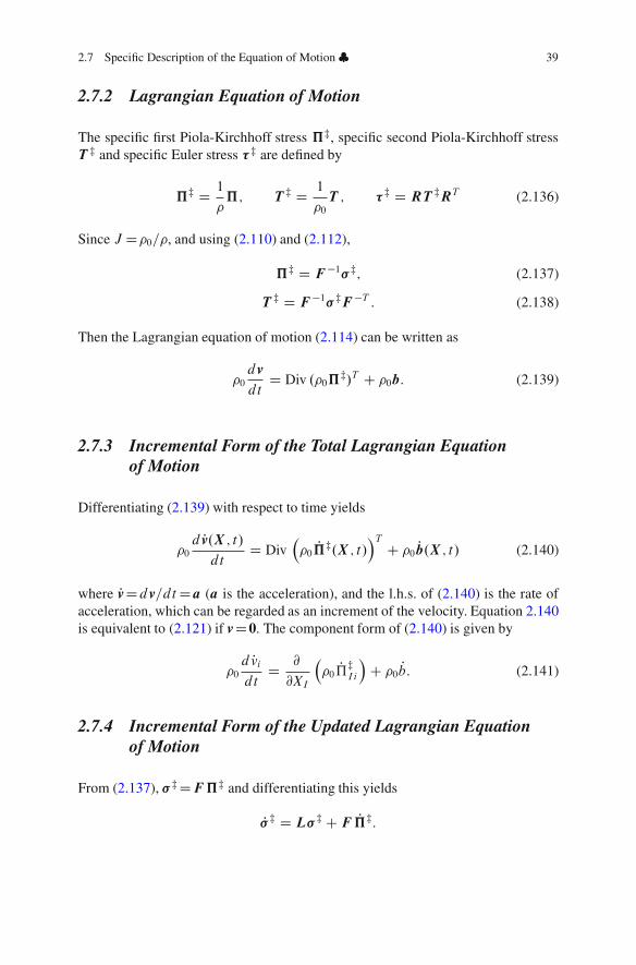
2.7.2 Lagrangian Equation of Motion
The specific first Piola-Kirchhoff stress …�, specific second Piola-Kirchhoff stressT � and specific Euler stress �� are defined by
…� D 1
…; T � D 1
0
T ; �� D RT �RT (2.136)
Since J D0=, and using (2.110) and (2.112),
…� D F �1� �; (2.137)
T � D F �1� �F �T : (2.138)
Then the Lagrangian equation of motion (2.114) can be written as
0
dvdt
D Div .0…�/T C 0b: (2.139)
2.7.3 Incremental Form of the Total Lagrangian Equationof Motion
Differentiating (2.139) with respect to time yields
0
d Pv.X ; t/
dtD Div
0
P…�.X ; t/�T C 0
Pb.X ; t/ (2.140)
where PvDdv=dt Da (a is the acceleration), and the l.h.s. of (2.140) is the rate ofacceleration, which can be regarded as an increment of the velocity. Equation 2.140is equivalent to (2.121) if vD0. The component form of (2.140) is given by
0
d Pvi
dtD @
@XI
0
P…�Ii
�C 0
Pb: (2.141)
2.7.4 Incremental Form of the Updated Lagrangian Equationof Motion
From (2.137), � � DF …� and differentiating this yields
P� � D L� � C F P…�:

40 2 Introduction to Continuum Mechanics
Thus we can define the specific nominal stress rate by
ı…� � F P…� D P� � � L� � (2.142)
On the other hand we have@
@XI
D FjI
@
@xj
:
Then (2.140) can be expressed as
0
d Pv.x; t/
dtD div
�0
ı…�.x; t/
�T
C 0Pb.x; t/ (2.143)
The l.h.s. of (2.143) can be written in the normal Eulerian description as
0
d Pv.x; t/
dtD 0
�@Pv@t
C v � div Pv�
: (2.144)
The component form of (2.143) is given as follows:
0
�@Pvi
@tC vj
@Pvi
@xj
�D @
@xj
�0
ı…
�j i
�C 0
Pbi : (2.145)
Equation 2.143 is equivalent to (2.131) if vD0; however, it is interesting to notethat the body force Pb is modified by , while each term of (2.143) is modifiedby 0.
2.8 Response of Materials: Constitutive Theory
The governing equations that control material responses are given by the mass con-servation law (2.97) and the equation of motion (2.104) if no energy conservation isconsidered. Note that the Cauchy stress is symmetric under the conservation law ofmoment of linear momentum. Furthermore, if the change of mass density is small(or it may be constant), the equation to be solved is given by (2.104). The unknownsin this equation are the velocity v (or displacement u in the small strain theory)and the stress � , i.e. giving a total of nine, that is, three for v (or u) and six for � .However, the equation of motion (2.104) consists of three components, therefore itcannot be solved, suggesting that we must introduce a relationship between v (or u)and � . The framework that provides this relationship is referred to as a constitutivetheory.

2.8 Response of Materials: Constitutive Theory 41
2.8.1 Fundamental Principles of Material Response
The constitutive law is fundamentally determined for each material, and it gives anempirical rule. To establish constitutive laws the following physical conditions arerequired:
Principle of determinism: The stress is determined by the history of the motionundergone by the body.
Principle of local action: The stress at a point is not influenced by far-field motions.Principle of frame indifference: The response of a material must be described under
the frame indifference (see Sect. 2.2.2).
The principle of frame indifference is sometimes called objectivity.Let a stress � be described as a function of a material point x in the deformed
body at time t :� D � .x; t/: (2.146)
As shown by (2.18), a coordinate transformation of the point x between twodifferent coordinate systems defined in the deformed body � is written as
x� D x�0 C Q.x � x0/; t� D t � a; (2.147)
and the frame indifference of the stress � is therefore
� �.x�; t�/ D Q.t/ � .x; t/ QT .t/: (2.148)
Because (2.147) implies that F �dX DQF dX , the deformation gradient F istransformed as
F � D Q F ; Q D Qije�i ˝ ej : (2.149)
Thus F is not frame indifferent. Some tensors introduced in Sect. 2.2.4 are verifiedas follows:
C � D F �T F � D .QF /T .QF / D F T F D C ; (2.150)
B� D F �F �T D .QF / .QF /T D Q B QT ; (2.151)
E� D F �F �T � I� D .QF /T .QF / � I D E ; (2.152)
L� D PF �.F �/�1 D .Q PF C PF Q/.QF /�1 D Q L QT C �; (2.153)
D� D 1
2
�L� C L�T
� D Q D QT ; (2.154)
W � D 1
2
�L� � L�T
� D Q W QT C �: (2.155)
Note that the right Cauchy-Green tensor C and the Green strain E are not frameindifferent, but frame invariant.
42 2 Introduction to Continuum Mechanics
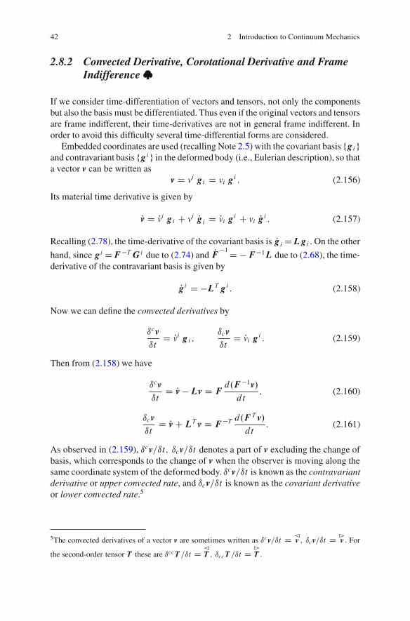
2.8.2 Convected Derivative, Corotational Derivative and FrameIndifference |
If we consider time-differentiation of vectors and tensors, not only the componentsbut also the basis must be differentiated. Thus even if the original vectors and tensorsare frame indifferent, their time-derivatives are not in general frame indifferent. Inorder to avoid this difficulty several time-differential forms are considered.
Embedded coordinates are used (recalling Note 2.5) with the covariant basis fgi gand contravariant basis fgi g in the deformed body (i.e., Eulerian description), so thata vector v can be written as
v D vi gi D vi gi : (2.156)
Its material time derivative is given by
Pv D Pvi gi C vi Pgi D Pvi gi C vi Pgi : (2.157)
Recalling (2.78), the time-derivative of the covariant basis is Pgi DLgi . On the other
hand, since gi DF �T G i due to (2.74) and PF �1 D � F �1L due to (2.68), the time-derivative of the contravariant basis is given by
Pgi D �LT gi : (2.158)
Now we can define the convected derivatives by
ıcvıt
D Pvi gi ;ıcvıt
D Pvi gi : (2.159)
Then from (2.158) we have
ıcvıt
D Pv � Lv D Fd.F �1v/
dt; (2.160)
ıcvıt
D Pv C LT v D F �T d.F T v/
dt: (2.161)
As observed in (2.159), ıcv=ıt; ıcv=ıt denotes a part of v excluding the change ofbasis, which corresponds to the change of v when the observer is moving along thesame coordinate system of the deformed body. ıcv=ıt is known as the contravariantderivative or upper convected rate, and ıcv=ıt is known as the covariant derivativeor lower convected rate.5
5The convected derivatives of a vector v are sometimes written as ıcv=ıt D C
v ; ıcv=ıt D B
v . For
the second-order tensor T these are ıccT =ıt D C
T ; ıccT =ıt D B
T .

2.8 Response of Materials: Constitutive Theory 43
For a second-order tensor T four convected derivatives are introduced as follows:
ıccT
ıtD PT ij gi ˝ gj ;
ıc�cTıt
D PT i�j gi ˝ gj ;
(2.162)ı�c
c T
ıtD PT �j
i gi ˝ gj ;ıccT
ıtD PTij g i ˝ gj :
Applying (2.78) and (2.158) and noting that LT Dgi ˝ Pgj yields
T ij Pgi ˝ gj D L T ij gi ˝ gj D LT ;
T ij gi ˝ Pgj D T ij gi ˝ Lgj D .T ij gi ˝ gj /LT D TLT ;
T i�j Pgi ˝ gj D L T i�j gi ˝ gj D LT ;
T i�j g i ˝ Pgj D �T i�j gi ˝ LT gj D �TL;
T�ji Pg i ˝ gj D �LT T
�ji gi ˝ gj D �LT T ;
T�ji g i ˝ Pgj D T
�ji gi ˝ Lgj D TLT ;
Tij Pg i ˝ gj D �LT Tij g i ˝ gj D �LT T ;
Tij gi ˝ Pgj D �Tij gi ˝ LT gj D �TL:
Thus (2.162) can be written as
ıccT
ıtD PT � LT � TLT D F
d.F �1TF �T /
dtF T ; (2.163)
ıc�cTıt
D PT � LT C TL D Fd.F �1TF /
dtF �1; (2.164)
ı�cc T
ıtD PT C LT T � TLT D F �T d.F T TF �T /
dtF T ; (2.165)
ıccT
ıtD PT C LT T C TL D F �T d.F T TF /
dtF �1: (2.166)
If an orthonormal coordinate transformation tensor Q .Q�1 DQT / is usedinstead of the deformation gradient F , the concept of the convected derivative canbe extended. That is, let �D PQQT be an antisymmetric rotation tensor generatedby Q as shown in (2.27), then the corotational derivative of a second-order tensorT due to Q is defined by
DQT
DtD PT C T � � �T D Q
d.QT TQ/
dtQT : (2.167)

44 2 Introduction to Continuum Mechanics
Here DQT =Dt represents an objective part of the time derivative of the second-order tensor T (the proof is similar to (2.170) as shown below). For example ifthe rotation tensor R and the spin tensor W are used instead of Q and �, we canintroduce the Zaremba-Jaumann rate as follows:
DT
DtD PT C T W � W T D R
d.RT TR/
dtRT : (2.168)
The material time derivative of a vector-valued or tensor-valued function is notalways objective as described above even if the original function is objective. It canbe said that the convected derivative and corotational derivative are introduced toensure objectivity of the time-derivative. For example we have
ıcvıt
�D dv�
dt� C L�T v� D d.Qv/
dtC .Q LT QT � �/ .Qv/ D Q
ıcvıt
(2.169)
ıccT
ıt
�D dT �
dt� C L�T T � C T �L�
D d.QTQT /
dtC .Q LT QT � �/ QTQT C QTQT .QLQT C �/
D QıccT
ıtQT : (2.170)
Note that the time derivative P� of Cauchy stress � is not objective, but the Zaremba-Jaumann rate D� =Dt is objective.
2.8.2.1 Spin of Eulerian Triads �E
Recall that the Eulerian triads fni g was introduced in (2.57). Let us define the spin�E of fni g by
Pni D �E ni ) �E D Pni ˝ ni D �E
ij ni ˝ ni ; �E
ij D ni � Pni : (2.171)
Since ni ˝ ni Di .i is the unit tensor for the deformed body), the time-differentialyields
�E D Pni ˝ ni D �ni ˝ Pni D �.�E/T :
This shows that �E is antisymmetric.We can define the following Lagrangian tensor �ER, which is the pull-back of
�E to the undeformed body by the rotation tensor R Dni ˝ N i :
�ER D RT �ER D �E
ij N i ˝ N i ) RT Pni D �ERN i (2.172)

2.8 Response of Materials: Constitutive Theory 45
2.8.2.2 Spin of Lagrangian Triads �L
Recall that the Lagrangian triads fN i g was introduced in (2.55). Let us also definethe spin �L of fN i g by
PN i D �L N i ) �L D PN i ˝ N i D �L
ij N i ˝ N i ; �L
ij D N i � PN i :
(2.173)
It is obvious that �L is antisymmetric. We can define the following Eulerian tensor�RL, which is the push-forward of �L to the deformed body by the rotation tensorR Dni ˝ N i :
�RL D R�LRT D �L
ij ni ˝ ni ) R PN i D �RLni : (2.174)
2.8.2.3 Eulerian Spin !R and Lagrangian Spin !RR
Time-differentiating RRT Di yields PRRT CR PRT D0, therefore the Eulerian spin!R and Lagrangian spin !RR, which is the pull-back of the Eulerian spin into theundeformed body, can be defined by
!R D PRRT D !Rij ni ˝ ni ; !RR D RT !RR D RT PR D !R
ij N i ˝ N i :
(2.175)On the other hand, because of (2.171) and the relation ni DRN i , we have
�E
ij D ni � Pnj D ni � . PRN i C R PN i / D ni � . PRRT /nj C ni � R�LN j
D ni � !Rnj C ni � �RLnj :
Thus the component form of the Eulerian spin is
!Rij D �
E
ij � �L
ij : (2.176)
The direct notations are given by
!R D �E � �RL; !RR D �ER � �L: (2.177)
2.8.2.4 Corotational Derivatives
Since the deformation gradient F can be written in terms of the polar decompositionas defined in (2.46), its time-differentiation gives
PF D PRU C R PU :
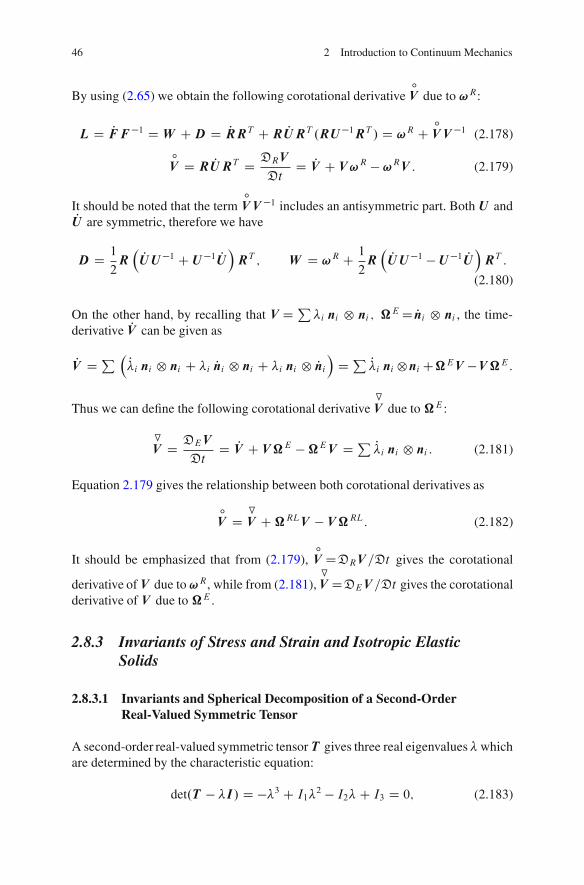
46 2 Introduction to Continuum Mechanics
By using (2.65) we obtain the following corotational derivativeıV due to !R:
L D PF F �1 D W C D D PRRT C R PU RT .RU �1RT / D !R C ıV V �1 (2.178)
ıV D R PU RT D DRV
DtD PV C V !R � !RV : (2.179)
It should be noted that the termıV V �1 includes an antisymmetric part. Both U and
PU are symmetric, therefore we have
D D 1
2R
PU U �1 C U �1 PU�
RT ; W D !R C 1
2R
PU U �1 � U �1 PU�
RT :
(2.180)
On the other hand, by recalling that V D P�i ni ˝ ni ; �E D Pni ˝ ni , the time-
derivative PV can be given as
PV D P P�i ni ˝ ni C �i Pni ˝ ni C �i ni ˝ Pni
�D P P�i ni ˝ni C�EV �V �E:
Thus we can define the following corotational derivativeOV due to �E :
OV D DEV
DtD PV C V �E � �EV D P P�i ni ˝ ni : (2.181)
Equation 2.179 gives the relationship between both corotational derivatives as
ıV D O
V C �RLV � V �RL: (2.182)
It should be emphasized that from (2.179),ıV DDRV =Dt gives the corotational
derivative of V due to !R, while from (2.181),OV DDEV =Dt gives the corotational
derivative of V due to �E .
2.8.3 Invariants of Stress and Strain and Isotropic ElasticSolids
2.8.3.1 Invariants and Spherical Decomposition of a Second-OrderReal-Valued Symmetric Tensor
A second-order real-valued symmetric tensor T gives three real eigenvalues � whichare determined by the characteristic equation:
det.T � �I/ D ��3 C I1�2 � I2� C I3 D 0; (2.183)

2.8 Response of Materials: Constitutive Theory 47
I1 D tr T ; I2 D 1
2
�.tr T /2 � tr T 2
; I3 D det T (2.184)
where I1; I2; I3 are the first, second and third principal invariants, respectively.The mean or volumetric tensor T and the deviatoric tensor T 0 are defined by
T D 1
3.tr T /I ; T 0 D T � T : (2.185)
Since the first invariant of the deviatoric tensor T 0 is zero (J1 D tr T 0 �0), its secondand third invariants are
J2 D 1
2T 0
ikT 0ki D 1
2tr .T 0/2; J3 D det T 0: (2.186)
Let us define the k-th moment NIk of a tensor T by
NIk D tr T k: (2.187)
Note 2.6 (Cayley-Hamilton Theorem). The well-known Cayley-Hamilton theoremstates that
C.T / D �T 3 C I1T2 � I2T C I3I D 0 (2.188)
which is similar to the characteristic equation (2.183).
Proof. Let us introduce an orthonormal basis feig .i D1; 2; 3/, and let the coefficientmatrix of T be Tlk (T DTlk el ˝ ek), which gives
T ek D Tlk el : (2.189)
We define a tensor B lk with tensorial components given by
B lk D TlkI � ılkT
(note that I Dıij ei ˝ ej ); thus (2.189) is equivalent to
B lkel D 0: (2.190)
We should recall that the adjoint A�ij of a regular matrix Aij is given by
A�km Alk D .det A/ ıml, and if we multiply the adjoint B�
km (with tensorialcomponents) by (2.190), we obtain
B�kmB lkel D det .B ij/ ımle l D 0; ) C.T / el D det .TlkI � ılkT / el D 0
(2.191)
48 2 Introduction to Continuum Mechanics
ıml D(
I if m D l
0 if m ¤ l:
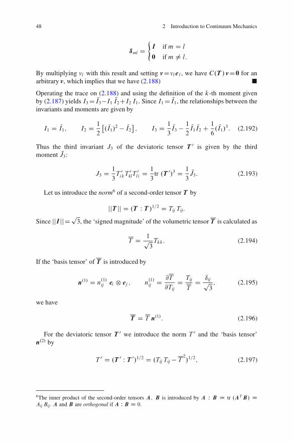
By multiplying vl with this result and setting vDvlel , we have C.T / vD0 for anarbitrary v, which implies that we have (2.188) �
Operating the trace on (2.188) and using the definition of the k-th moment givenby (2.187) yields I3 D NI3�I1
NI2CI2 I1. Since I1 D NI1, the relationships between theinvariants and moments are given by
I1 D NI1; I2 D 1
2
�. NI1/
2 � NI2
; I3 D 1
3NI3 � 1
2NI1
NI2 C 1
6. NI1/
3: (2.192)
Thus the third invariant J3 of the deviatoric tensor T 0 is given by the thirdmoment NJ3:
J3 D 1
3T 0
ikT 0klT
0li D 1
3tr .T 0/3 D 1
3NJ3: (2.193)
Let us introduce the norm6 of a second-order tensor T by
jjT jj D .T W T /1=2 D Tij Tij:
Since jjI jjDp3, the ‘signed magnitude’ of the volumetric tensor T is calculated as
T D 1p3
Tkk: (2.194)
If the ‘basis tensor’ of T is introduced by
n.1/ D n.1/ij ei ˝ ej ; n
.1/ij D @T
@TijD Tij
TD ıijp
3; (2.195)
we have
T D T n.1/: (2.196)
For the deviatoric tensor T 0 we introduce the norm T 0 and the ‘basis tensor’n.2/ by
T 0 D .T 0 W T 0/1=2 D .Tij Tij � T2/1=2; (2.197)
6The inner product of the second-order tensors A; B is introduced by A W B D tr .AT B/ DAij Bij. A and B are orthogonal if A W B D 0.

2.8 Response of Materials: Constitutive Theory 49
n.2/ D n.2/ij ei ˝ ej ; n
.2/ij D @T 0
@T 0ij
D T 0ij
T 0 (2.198)
) T 0 D T 0n.2/: (2.199)
Lode’s angle T of T and the Lode parameter yT can be introduced by
yT D cos .3T / D 3p
3J3
2 .J2/3=2D p
6 tr .n.2//3: (2.200)
If the tensor of Lode’s angle is defined by
T D T n.3/; (2.201)
its ‘basis tensor’ n.3/ Dn.3/ij ei ˝ ej can be calculated as
n.3/ij D T 0 @T
@TijD T 0 @T
@yT
@yT
@TijD
p6
sin .3� /
�n
.2/ij tr .n.2//3 � n
.2/
ik n.2/
kj C 1p3
n.1/ij
�
) n.3/ Dp
6
sin .3� /
�n.2/tr .n.2//3 � .n.2//2 C 1p
3n.1/
�(2.202)
where we used the relationship tr .n.2//2 D1.The basis tensors n.1/; n.2/; n.3/ are mutually orthogonal in the sense of
n.˛/ W n.ˇ/ D ı˛ˇ: (2.203)
Thus the second-order real-valued symmetric tensor T is written in orthogonalcomponents by
T D T.˛/ n.˛/ .˛ W summed/ (2.204)
where we setT.1/ D T ; T.2/ D T 0; T.3/ D T :
The result (2.204) is referred to as the spherical decomposition of T .
2.8.3.2 Geometrical Interpretation of Spherical Decomposition in thePrincipal Space
Let the eigenvalue representation of the second-order real-valued symmetric tensorT be given by
T D3X
iD1
Tie0i ˝ e0
i :

50 2 Introduction to Continuum Mechanics
Fig. 2.11 Deviatoric,volumetric and Lode’scomponents in the principalspace
Then the volumetric, deviatoric and Lode’s components T , T 0, T are as shownin Fig. 2.11 together with the base tensors n.˛/ .˛ D1; 2; 3/ (since the tensors inthe principal space are termed ‘vectors’, we will use this designation). T is theprojection of T on the diagonal axis T1 DT2 DT3 (which is referred to as thehydrostatic axis for the stress). The difference vector T � T gives the deviatoricvector T 0. The orthogonal plane to T including the vector T 0 is referred to as the…-plane. . If the projected axis of T1 on the …-plane is T 0
1 , the angle between T 01
and T 0 gives the Lode’s angle T .This implies that, by spherical decomposition, cylindrical polar coordinates are
introduced in terms of the ‘hydrostatic’ axis.
2.8.3.3 Spherical Decompositions of Stress and Strain and the Responseof an Isotropic Elastic Solid
The stress � is a second-order real-valued symmetric tensor, and the sphericaldecomposition is given as follows:
N� D I �1 I=3 Volumetric stress
I �1 D tr .� / First invariant of stress
N� D I �1 =
p3 Magnitude of volumetric stress
� 0 D � � N� Deviatoric stress� 0 D k� 0k D .� 0 W � 0/1=2 Magnitude of deviatoric stress� D 1
3cos�1f3p
3J �3 =2.J �
2 /3=2g Lode’s angle for stressJ �
2 D � 0 W � 0=2 Second invariant of deviatoric stressJ �
3 D det .� 0/ Third invariant of deviatoric stress
For the strain " we can introduce the spherical decomposition as follows:
N" D I "1 I=3 Volumetric strain
I "1 D tr ."/ First invariant of strain
N" D I "1 =
p3 Magnitude of volumetric strain
"0 D " � N" Deviatoric strain

2.8 Response of Materials: Constitutive Theory 51
"0 D k"0k D ."0 W "0/1=2 Magnitude of deviatoric strain" D 1
3cos�1f3p
3J "3 =2.J "
2 /3=2g Lode’s angle for strainJ "
2 D "0 W "0=2 Second invariant of deviatoric strainJ "
3 D det ."0/ Third invariant of deviatoric strain
If a material body is an isotropic solid, the stress and strain are decomposed byusing the same basis n.˛/:
� D N� C � 0 C � ; N� D N� n.1/; � 0 D � 0n.2/; � D � 0� n.3/; (2.205)
" D N" C "0 C " ; N" D N" n.1/; "0 D "0n.2/; " D "0" n.3/; (2.206)
and the linear elastic response is written in terms of the volumetric and deviatoriccomponents independently (cf. Note 2.7). Thus, referring to Fig. 2.11, the responsegives a state that is symmetric about the hydrostatic axis as follows:
N� D 3� N"; � 0 D 2�"0: (2.207)
The coefficients �; � are called Lame’s constants. Then the response of the linearelastic solid, called the Hookean solid, is written as
�ij D �"kk ıij C 2� "ij: (2.208)
Young’s modulus E and Poisson’s ratio � are related to Lame’s constants �; �, theshear modulus G and bulk modulus K as
� D E�
.1 C �/.1 � 2�/; � D E
2.1 C �/D G; K D � C 2
3� D E
3.1 � 2�/:
(2.209)
Note 2.7 (Lode’s angle and the response of isotropic solids). If the elastic responseof solids is written using Hooke’s law as
� D De "; (2.210)
the most general form of the fourth order tensor De for isotropic materials isgiven by
Deijkl D �ıijıkl C �.ıikıjl C ıil ıjk/ C �.ıikıjl � ıil ıjk/ (2.211)
(cf. Malvern 1969, pp. 277). Since � and " are symmetric (�ij D�j i , "ij D"j i ), wehave the condition � D0, which causes no change in the Lode’s angle componentfor isotropic solids, and the axi-symmetric response with respect to the hydrostaticaxis. Another result is that there exist two independent elastic constants, althoughthe number of eigenvalues of stress and strain is three.
52 2 Introduction to Continuum Mechanics
We also note that a tensor function defined as
Deijkl D �ıijıkl C �ıikıjl C �ıilıjk (2.212)
is also isotropic (Little 1973; Spencer 2004). The constitutive equation (2.210) nowbecomes
� D �ıij"kk C �"ij C �"ij: (2.213)
Since "ij D"j i , no generality is lost by setting �D� such that � D�ıij"kkC2�"ij. �
The inverse relation of (2.208) is
"ij D � �
E�kk ıij C 1 C �
E�ij: (2.214)
For two dimensional problems we can consider two idealized states: theplane strain state where "zz D"xz D"yz D0 and the plane stress state in which�zz D�xz D�yz D0. Under these conditions, Hooke’s law is rewritten for the vectorforms of stress and strain as
� D De "; � D Œ�xx �yy �xy�T ; " D Œ"xx "yy �xy�T (2.215)
Plane strain W De D E.1 � �/
.1 C �/.1 � 2�/
266664
1�
1 � �0
�
1 � �1 0
0 01 � 2�
2.1 � �/
377775 (2.216)
Plane stress W De D E
1 � �2
2664
1 � 0
� 1 0
0 01 � �
2
3775 : (2.217)
Here we have used the engineering shear strain �xy D 2"xy . The representation ofstress and strain given by (2.215) is referred to as the contracted form.
If the material body involves an initial stress � 0 and/or initial strain "0, Hooke’slaw is transformed to
� D De." C "0/ C � 0 (2.218)
If the initial strain is caused by a temperature difference T � T0, we have "0 D˛.T � T0/i for an isotropic material body, therefore the above equation becomes
"ij D � �
E�kk ıij C 1 C �
E�ij C ˛.T � T0/ ıij (2.219)
where T0 is the reference temperature and ˛ is the thermal expansion coefficient.
2.8 Response of Materials: Constitutive Theory 53
Substituting Hooke’s law (2.208) into the equation of motion (2.104) yields thefollowing Navier’s equation where the unknown variable is the displacement u:
d 2ui
dt2D .� C �/
@2uj
@xi @xj
C �@2ui
@xj @xj
C bi : (2.220)
Note 2.8 (Solid and fluid). The term “solid” is used for the material body where theresponse is between the stress � and the strain " or between the stress increment d�
and the strain increment d". The term “fluid” is used for the material body wherethe response is between the stress � and the strain rate P" (or the stretch tensor D).For a fluid we have to introduce a time-integration constant, which is referred to asthe pressure p. �
2.8.4 Newtonian Fluid
For simplicity, we describe the equations without mass density . Since the specificstress � �.x; t/ is given in terms of an Eulerian description, we treat here thesimplest response for that description. To satisfy the principle of determinism andthe principle of local action mentioned in the previous section, the stress � �.x; t/
can be written in terms of v and rv:
� � D � �.v; rv/: (2.221)
The frame indifference of the stress � �.x; t/ is a natural conclusion of Newtonianmechanics in that the force vector is frame indifferent. Since the stretch tensor D isframe invariant by (2.154), we use D instead of rv. From (2.27) we have
v� D dx�0
dtC dQ
dt.x � x0/ C Qv:
Therefore the frame indifference requires the following condition:
� ��.v�; D�/ D Q� �
Px�0 C PQ.x � x0/ C Qv; QDQT
�QT
We define x�0 as
Px�0 D � PQ.x � x0/ � Qv
Then we can see that if we have
Q� �.D/QT D � �.QDQT / ) � � D � �.D/ (2.222)

54 2 Introduction to Continuum Mechanics
the fundamental principles mentioned in the previous section are satisfied. Since D
is symmetric and non-negative definite, the most general form (Truesdell and Noll1965, pp. 32; Malvern 1969, pp. 194) can be given by
� D � � D �0i C �1D C �2D2 (2.223)
where �i .i D0; 1; 2/ are functions of the invariants I Di .i D1; 2; 3/ of D:
�i D �i .ID1 ; I D
2 ; I D3 /: (2.224)
The invariants I Di are calculated by the following characteristic equation for
specifying the eigenvalue �:
det .D � �i / D ��3 C I D1 �2 � I D
2 �1 C I D3 D 0; (2.225)
I D1 D tr D D r � v;
I D2 D 1
2
h.I D
1 /2 � OI D2
i; OI D
2 D tr .D2/;
I D3 D det D
We omit the third term of the r.h.s. of (2.223) so as to linearize it:
� D � � D .�p C � tr D/ i C 2�D (2.226)
where p is the pressure and �; � are viscosities (� is the shearing viscosity, and� D�C2�=3 is the bulk viscosity: described below). The pressure p appears in thisequation because v (and also D) is a material time derivative of the position vectorx of a material point in the deformed body, which needs an integration constant;this corresponds to the pressure. Note that usually the “pressure” is set positive forcompression, therefore a negative sign of p appears in (2.226). Materials that behaveas (2.226) are referred to as Newtonian fluids.
Let us resolve the stress � and stretch tensor D into direct sums of volumetricand deviatoric components, respectively:
� D N� C � 0; (2.227)
N� D 1
3.tr � / i ; � 0 D � � N� ; (2.228)
D D D C D0; (2.229)
D D 1
3.tr D/ i ; D0 D D � D: (2.230)
N� and D are the volumetric components of each tensor, and � 0 and D0 are thedeviatoric (or shearing) components. The volumetric component is orthogonal to

2.8 Response of Materials: Constitutive Theory 55
the deviatoric one in the following sense:
N� W � 0 D tr� N� T � 0� D 0; D W D0 D tr
D
TD0� D 0: (2.231)
Since .r � v/I D3D, we can rewrite (2.226) as
N� C � 0 D �pi C 3
�� C 2
3�
�D C 2�D0
Recalling the orthogonality of the volumetric and deviatoric components, eachcomponent will give an independent response:
N� D �pi C 3�D; � 0 D 2�D0 (2.232)
This is a direct result of the response of an isotropic linear fluid. In this equation theconstant
� D � C 2
3� (2.233)
gives the bulk (i.e., volumetric) viscosity and � is the shearing viscosity.Thus the most fundamental constitutive law for a fluid is understood to be given
as a Newtonian fluid defining a linear relationship between the stress � and thestretch tensor D (recall that the stretch tensor D is equal to the strain rate for thesolid with small strain). The constitutive law is also called Stokes’ law, and can berewritten as
�ij D �p ıij C � Dkk ıij C 2� Dij (2.234)
Substituting Stokes’ law (2.234) into the equation of motion (2.104) under theEulerian description yields the following equation of motion for the unknownvelocity v:
�@vi
@tC vj
@vi
@xj
�D � @p
@xi
C .� C �/@2vj
@xi @xj
C �@2vi
@xj @xj
C bi (2.235)
These are the Navier-Stokes equations. If the body force can be set as bD � r� bya potential �, we define
p� D p C �; (2.236)
and the Navier-Stokes equations can be written as
�@vi
@tC vj
@vi
@xj
�D �@p�
@xi
C .� C �/@2vj
@xi @xj
C �@2vi
@xj @xj
: (2.237)

56 2 Introduction to Continuum Mechanics
If the fluid is incompressible, the condition (2.99) applies and we have
�@vi
@tC vj
@vi
@xj
�D � @p
@xi
C �@2vi
@xj @xj
C bi : (2.238)
2.9 Small Strain Viscoelasticity Theory
The one-dimensional viscoelastic response is schematically illustrated in Fig. 2.12.Note that the ‘stress relaxation’ is a phenomenon that appears under a constant straincondition, while ‘creep’ is one that appears under a constant stress condition. Theresponse shown is represented by a model based on an excitation-response theorytogether with a data management procedure. Note that we assume an isotropicmaterial response.
2.9.1 Boltzmann Integral and Excitation-response Theory
The viscoelastic response is commonly described by using a form of Boltzmann’shereditary integral, referred to as the excitation-response theory (Gurtin andSternberg 1962; Yamamoto 1972; Christensen 2003).
Fig. 2.12 Viscoelastic response

2.9 Small Strain Viscoelasticity Theory 57
Let us consider a step input function
x.t/ D(
0 for t < 0;
x0 D constant for t > 0:(2.239)
The corresponding response to this input can be written as
y.t/ D �.t/ x0 (2.240)
where �.t/ is referred to as the after-effect function (Fig. 2.13a) which satisfies thecondition
�.t/ D 0 for t < 0:
If the input x.t/ is given by a collection of step functions as shown in Fig. 2.13b,the response is written as
y.t/ DX
i
�.t � ti /xi : (2.241)
Then for a general form of the input function x.t/, we have
y.t/ DZ t
�1�.t � s/
dx.s/
dsds: (2.242)
This is referred to as Boltzmann’s superposition principle.
(a) After–effect function (b) Superposition principle
Fig. 2.13 Boltzmann’s hereditary integral

58 2 Introduction to Continuum Mechanics
Integrating (2.242) by parts yields
y.t/ D �.0C/ x.t/ CZ t
�1d�.t � s/
dsx.s/ ds �
Z t
�1�.t � s/ x.s/ ds (2.243)
where�.0C/ D lim
t!C0�.t/
and
�.t � s/ D d�.t � s/
dsC ı.s/ �.s/ (2.244)
is referred to as the response function.7
2.9.2 Stress Relaxation and the Relaxation Spectra:Generalized Maxwell Model
First we consider a simple uniaxial response. If a strain " is given by
".t/ D(
0 for t < 0;
"0 for t > 0;(2.245)
we write the relaxation stress as
�.t/ D E.t/"0; E.t/ D 0 for t < 0 (2.246)
where the after-effect function E.t/ is referred to as the relaxation function.Following Boltzmann’s principle presented previously, if an input ".t/ is given, theresponse can be written as
�.t/ DZ t
�1E.t � s/
d".s/
dsds D
Z t
�1ƒ.t � s/ ".s/ ds: (2.247)
The response of a viscoelastic material is generally represented as a modelcontaining a combination of elastic, viscous and pure stress-relaxation properties.Then the relaxation function can be written as
E.t/ D E0 C �1 ı.t/ C E.t/ (2.248)
7The definition of the ı-function is given byR
� dy ı.y � x/f .y/ D f .x/.
2.9 Small Strain Viscoelasticity Theory 59
where E.t/ is a smooth, monotonically decreasing function such that
E.0/ D � < C1; E.C1/ D 0;
and can be represented by a Laplace transformation:
E.t/ DZ 1
0
N.s/ exp.�st/ ds: (2.249)
In order to provide a discrete approximation of this function, the variable s ischanged into � by � D1=s. Then (2.249) can be written as
E.t/ DZ 1
0
H.�/ exp.�t=�/ d.ln �/; (2.250)
H.�/ D 1
�N
�1
�
�; (2.251)
and H.�/ is referred to as the relaxation spectrum.Substituting (2.250) into (2.247) and changing the order of integration, we have
�.t/ D �0.t/ C �1.t/ CZ 1
0
�.t; �/ d.ln �/; (2.252)
�.t; �/ D H.�/
Z t
�1exp .�.t � s/=�/
d".s/
dsds; (2.253)
�0.t/ D E0 ".t/; �1.t/ D �1d".t/
dt: (2.254)
Differentiating (2.253)8 we obtain
H.�/d".�/
dtD d
dt�.t; �/ C 1
��.t; �/: (2.255)
8Leibnitz rule: If we have an integral of a continuous function f such as
�.x/ DZ h1.x/
h0.x/
f .x; �/ d�;
and if h1.x/ and h0.x/ are continuous on R D f .x; �/ W a � x � b; c � � � d g, then
d�.x/
dxD f .x; h1.x//
dh1.x/
dx� f .x; h0.x//
dh0.x/
dxC
Z h1.x/
h0.x/
@f .x; �/
@xd�
(see, e.g., Protter and Morrey 1977, pp. 284).

60 2 Introduction to Continuum Mechanics
A mechanical representation of a simple Maxwell model is shown in Fig. 2.14a andcan be indicated in the same form as (2.255): i.e.
Ed"
dtD d�
dtC 1
��
where E and � are the elastic and viscous constants, respectively, and � D�=E isreferred to as the relaxation time. Thus we understand that (2.252) gives a synthesisof each spectral response corresponding to � , and this suggests that, for a discretecase, the generalized Maxwell model can be represented by Fig. 2.15a.
If the material is isotropic, the response can be written in both deviatoric andvolumetric forms:
s.t/ D 2
Z t
�1G.t � s/
de.s/
dsds; N� .t/ D 3
Z t
�1K.t � s/
d N".s/
dsds (2.256)
where
G.t/ D G0 C �s1 ı.t/ C G.t/; K.t/ D K0 C �v1 ı.t/ C K.t/; (2.257)
G.t/ DZ 1
0
ˆs.�/ exp.�t=�/ d.ln �/; K.t/ DZ 1
0
ˆv.�/ exp.�t=�/ d.ln �/:
(2.258)
a b
Fig. 2.14 (a) Maxwellmodel, (b) Kelvin-Voigtmodel
a b
Fig. 2.15 (a) GeneralizedMaxwell model, (b)generalized Kelvin-Voigtmodel

2.9 Small Strain Viscoelasticity Theory 61
Since � .t/Ds.t/C N� .t/, the total response can be represented as
� .t/ DZ t
�1
�2G.t � s/
de.s/
dsC 3K.t � s/
d N".s/
ds
�ds D
Z t
�1D.t�s/
d".s/
dsds:
(2.259)
2.9.3 Creep and the Retardation Spectra: GeneralizedKelvin-Voigt Model
Let us consider a simple uniaxial creep response. If a creep stress � is given by
�.t/ D(
0 for t < 0;
�0 for t > 0;(2.260)
and the corresponding strain response is written as
".t/ D J.t/ �0; J.t/ D 0 for t < 0; (2.261)
then for a general input �.t/ the strain response can be represented as
".t/ DZ t
�1J.t � s/
d�.s/
dsds D
Z t
�1�.t � s/ �.s/ ds (2.262)
where J.t/ is referred to as creep function.In the same way as we did for stress relaxation, we combine the instantaneous
elastic, viscous and pure stress-relaxation properties, and write the response as
J.t/ D J1 C t
�0
C J .t/ (2.263)
where J1 D1=E1. Since NJ .t/ is a smooth, monotone decreasing function, we have
J .0/ D 0; J .C1/ D < C1:
Therefore it can be represented by a Laplace transformation:
J .t/ DZ 1
0
M.s/ .1 � exp.�st// ds DZ 1
0
L.�/ .1 � exp.�t=�// d.ln �/;
(2.264)
L.�/ D 1
�M
�1
�
�: (2.265)
L.�/ is referred to as the retardation spectrum.

62 2 Introduction to Continuum Mechanics
Substituting (2.264) into (2.262) and changing the order of integration, we have
".t/ D "1.t/ C "0.t/ CZ 1
0
".t; �/ d.ln �/ (2.266)
".t; �/ D L.�/
Z 1
0
.1 � exp.�.t � s/=�//d�.s/
dsds; (2.267)
"1.t/ D J1 �; "0.t/ D 1
�0
Z t
�1�.s/ ds: (2.268)
Differentiating (2.267), we obtain
L.�/�.t/ D �d
dt".t; �/ C ".t; �/ (2.269)
The response of a simple one-unit Kelvin-Voigt model shown by Fig. 2.14b can bewritten in a form similar to (2.269) as
J� D �d"
dtC "
where J D1=E and � are the elastic compliance and viscous constant, respectively,and � D�=E is referred to as the retardation time. Thus we can see that (2.266)gives a synthesis of each spectral response corresponding to � , and this suggeststhat for a discrete case the generalized Kelvin-Voigt model can be represented byFig. 2.15b.
If the material is isotropic, the response can be given separately for the deviatoricand volumetric deformations as follows:
e.t/ D 1
2
Z t
�1B.t � s/
ds.s/
dsds; N".t/ D 1
3
Z t
�1C.t � s/
d N� .s/
dsds (2.270)
where
B.t/ D B1 C t
�s0
C B.t/; C.t/ D C1 C t
�v0
C C.t/ (2.271)
B.t/ DZ 1
0
‰s.�/ .1 � exp.�t=�// d.ln �/;
C .t/ DZ 1
0
‰v.�/ .1 � exp.�t=�// d.ln �/: (2.272)
Since ".t/De.t/C N".t/, the total response is thus represented as
".t/ DZ t
�1
�1
2B.t � s/
ds.s/
dsC 1
3C.t � s/
d N� .s/
ds
�dsD
Z t
�1C .t�s/
d� .s/
dsds:
(2.273)

2.9 Small Strain Viscoelasticity Theory 63
2.9.4 Relaxation and Retardation Spectra and TheirAsymptotic Expansion
The k-th derivative of (2.249) yields
E.k/
.t/ D d kE.t/
dtkD .�1/k
Z 1
0
N.s/sk exp.�st/ ds
where E.k/
implies the k-time differentiation of E. Since sk exp.�st/ shows thepeak value at s Dk=t and the value increases with k, we can replace it by theı-function so that we have
Z 1
0
sk exp.�st/ ds D kŠ
tkC1:
Therefore we set
E.k/
.t/ D .�1/k kŠ
tkC1
Z 1
0
N.s/ı.s � k=t/ ds D .�1/k kŠ
tkC1N.k=t/:
Now we change the variable as t Dk=s, and obtain
E.k/
.k=s/ D .�1/kskC1 kŠ
kkC1N.s/:
This gives a function N.s/, and, when k ! 1, we have the following asymptoticform:
N.s/ D limk!1
.�1/k
kŠ
�k
s
�kC1
E.k/
.k=s/:
Since E is a function of k=s, and using (2.251) we have a function H.�/ insteadof N.s/9:
H.�/ D 1
�N
�1
�
�D lim
k!1.�1/k
.k � 1/Š.k�/k E
.k/.k�/: (2.274)
Equation 2.274 shows that the relaxation spectrum H.�/ can be approximated by
H1.�/ D ��@E.�/
@�; H2.�=2/ D �2 @2E.�/
@�2; H3.�=3/ D ��3
2
@3E.�/
@�3; � � �
When using actual experimental data, the differentiation frequently involvessome numerical errors, therefore we can use either H2 or, more often, H1 for thespectral approximation. The practical procedures will be given in a later section.
9Note that the differentiation implies E.k/
.k�/ D dkE.k�/
d.k�/k. Others are the same.

64 2 Introduction to Continuum Mechanics
The most important advantage of this procedure is that we can determine thespectral points that govern the corresponding viscoelastic response, which givestheir coefficients, specified by the least squares method.
The retardation spectrum L.�/ of (2.264) is written as
L.�/ D limk!1
.�1/kC1
.k � 1/Š.k�/k NJ .k/.k�/: (2.275)
For an isotropic material the relaxation spectra are given by
ˆs.�/ D limk!1
.�1/k
.k � 1/Š.k�/k G
.k/.k�/; ˆv.�/ D lim
k!1.�1/k
.k � 1/Š.k�/k K
.k/.k�/;
(2.276)and the retardation spectra are
‰s.�/ D limk!1
.�1/k
.k � 1/Š.k�/k B
.k/.k�/; ‰v.�/ D lim
k!1.�1/k
.k � 1/Š.k�/k C
.k/.k�/:
(2.277)
2.9.5 Experiments for Determining Viscous Properties
Several experiments are used to determine the viscoelastic properties of a material:creep tests (stress D constant), relaxation tests (strain D constant) and a constantstress rate test. Figure 2.12 shows the loading paths of each test for the one-dimensional case.
We first determine the creep function J.t/ based on the results of a creep test:If the creep stress is given by (2.260), the response is given by (2.261), therefore".t/DJ.t/�0. Let us assume that the relaxation spectrum is represented by the firstapproximation of (2.275), i.e.,
L.�/ D ��@J .�/
@�:
By substituting (2.261) into this result we have
L.�/ D � 1
�0
�@".�/
@�: (2.278)
We can then plot the values of (2.278) calculated by the creep curve shown, forexample, in Fig. 2.16. In this figure we specify discrete values �1; �2; : : :. Since thediscrete representation of (2.264) is given by
J .t/ DX
i
Ji .1 � exp.�t=�i // ; Ji D L.�i / ln �i ; (2.279)

2.9 Small Strain Viscoelasticity Theory 65
Fig. 2.16 Implication ofretardation spectrum
we can substitute the above �i ’s into (2.279), and, using (2.261) and (2.263), weobtain the following:
".t/ D"
J1 C t
�0
CX
i
Ji .1 � exp.�t=�i //
#�0: (2.280)
We now need a procedure to determine �0. From (2.280) the slope at the finalelapsed time t� is given by
1
�0
d"
dt
ˇˇtDt�
DX Ji
�i
exp.�t�=�i / C 1
�0
: (2.281)
Thus if �i � t�, we can specify the slope 1=�0. If �i � t�, the reader is referred toAkagi (1980) for details of the method to specify �0.
If �i .i D1; 2; : : :/ and �0 are known, J1 and Ji .i D1; 2; : : :/ can be specifiedby a linear least squares method. That is, setting the error estimate as
… D 1
2�2
0
"J1 C t
�0
CX
i
Ji .1 � exp.�t=�i //
#2
; (2.282)
J1 and Ji can be calculated by solving the following simultaneous equations:
@…
@J1D 0;
@…
@Ji
D 0; i D 1; 2; : : : (2.283)
For an isotropic material, the creep functions B.t/ and C.t/ are determined usingthe same procedure. For an axisymmetric triaxial stress state, let �1 be the axialstress, �3.< 0/ (with �2 D�3) the confining pressure, "1 the measured axial strainand "3 the measured lateral strain. Then setting
s11 D 2
3.�1 � �3/ D �2s22 D �2s33 � q0; s23 D s31 D s13 D 0;
N� D 1p3
.�1 C 2�3/ � p0;

66 2 Introduction to Continuum Mechanics
e11 D 2
3."1 � "3/ D �2e22 D �2e33 � "s; e23 D e31 D e13 D 0;
N" D 1p3
."1 C 2"3/ � "v;
we have the following deviatoric and volumetric creep responses:
"s.t/ D 1
2B.t/ q0; "v.t/ D 1
3C.t/ p0: (2.284)
Due to (2.277), the first approximations of the relaxation spectra of each componentare given by
‰s.�s/ D � 2
q0
�s @"s.�s/
@�s; ‰v.� v/ D � 3
p0
� v @"v.� v/
@� v: (2.285)
Therefore the discrete relaxation times �s1 ; �s
2 ; : : : ; � v1 ; � v
2 ; : : : can be obtained bycreep curves (similar to Fig. 2.16). This gives the discrete forms of (2.272) as
B.t/ DX
i
Bi
�1 � exp.�t=�s
i /�
; Bi D ‰s.�si / ln �s
i
C .t/ DX
i
Ci
�1 � exp.�t=� v
i /�
; Ci D ‰v.� vi / ln � v
i
(2.286)
and we obtain
"s.t/ D 1
2
"B1 C t
�s0
CX
i
Bi
�1 � exp.�t=�s
i /�#
q0
"v.t/ D 1
3
"C1 C t
�v0
CX
i
Ci
�1 � exp.�t=� v
i /�#
p0:
(2.287)
Under the condition �si ; � v
i � t�, �s0 and �v
0 can be specified by using the slopes ofthe creep curves at the final time stage t� by
2
q0
d"s
dt
ˇˇtDt�
:D 1
�s0
;3
p0
d"v
dt
ˇˇtDt�
:D 1
�v0
: (2.288)
The coefficients B1 and Bi .i D1; 2; : : :/, C1 and Ci .i D1; 2; : : :/ can becalculated by the least squares method where the error estimates are given by
…s D 1
8q2
0
"B1 C t
�s0
CX
i
Bi
�1 � exp.�t=�s
i /�#2
;
…v D 1
18p2
0
"C1 C t
�v0
CX
i
Ci
�1 � exp.�t=� v
i /�#2
;

2.10 Small Strain Plasticity: Flow Theory 67
which gives the simultaneous equations
@…s
@B1D 0;
@…s
@Bi
D 0; (2.289)
@…v
@C1D 0;
@…v
@Ci
D 0: (2.290)
Finally, we can see the relationship between the response given by the hereditaryintegral form and that given by conventional creep laws such as the logarithmic form
".t/ D a C b ln t; (2.291)
and Norton’s power law"
tD a �n: (2.292)
Differentiating (2.291) yields
td"
dtD b:
Therefore the logarithmic creep law employs an averaged relaxation spectrum forall elapsed time (i.e., only one time-dependent mechanism is assumed) as shown inFig. 2.16, which may cause difficulty under real, complex situations such as the longterm behavior of rock. On the other hand the power law (2.292) gives
td"
dtD t .a�n
0 /
for a creep stress �0, which implies a linear distribution of the spectra (Fig. 2.16).
2.10 Small Strain Plasticity: Flow Theory
In this book we are considering porous materials. Therefore, the stress treated heremust be an effective stress � 0 D� CpI where � is the total stress, and p is thepore fluid pressure. Note that in this section we are using the sign conventionfor stresses adopted in continuum mechanics, therefore the tension stress/strain isconsidered positive, and the pore fluid pressure is positive, since � 0 D�CpI (detailsare described in Chap. 6). In this Section we denote the stress as � instead of theeffective stress � 0 for simplicity. Readers can see that all results in this section alsowork for the effective stress. It should be noted that in this section the deviatoricstress is denoted as s whereas in other expositions the deviatoric stress is written as� 0. Similarly, the deviatoric strain is denoted as e.
68 2 Introduction to Continuum Mechanics
Symbols and notations used in this section are given below:
� (Total) stress tensor (tension: +)I1 D tr .� / D �ii First invariant of stressI2 D f.tr � /2 � tr .� 2/g=2 Second invariant of stressI3 D det.� / Third invariant of stressN� D tr .� /I=3 Volumetric stress tensor (tension, +)N� D tr .� /=
p3 Magnitude of volumetric
stress (tension, +)s D � � N� Deviatoric stress tensors D jsj D .sij sij/
1=2 Norm of deviatoric stress� D 1
3cos�1Œ3
p3 J �
3 =f2.J �2 /3=2g� Lode’s angle for stress
J2 D sijsij=2 D 2s2 Second invariant of deviatoric stressJ3 D det.s/ Third invariant of deviatoric stressd" D d"e C d"p Strain increment tensord"e Elastic strain increment tensord"p Plastic strain increment tensord N"p D tr .d"p/I=3 Volumetric plastic strain increment
tensord N"p D tr .d"p/=
p3 Magnitude of volumetric plastic
strain incrementdep D d"p � d N"p Deviatoric plastic strain increment
tensordep D jdepj D .de
pij de
pij /
1=2 Norm of deviatoric plasticstrain increment
� Hardening parameter
The result of a simple tension experiment for a metal is schematically shownin Fig. 2.17 with axes of axial stress �1 and axial strain "1 or deviatoric stress s
and deviatoric strain e. In metals the volumetric plastic strain can generally beignored ( N"p D0); therefore we can treat the behavior as a uniaxial response. Onthe other hand, the shearing behavior of geomaterials is inevitably accompanied byvolume changes that are plastic, therefore we have to modify the original flow theorydeveloped for metallic materials (Kachanov 2005; Lubliner 1990). Note that in smallstrain plasticity we assume that the plastic increment d" can be decomposed intoincremental elastic and plastic components:
d" D d"e C d"p: (2.293)
2.10.1 Yield Function and Hardening Law
Let us denote the yield condition by
f .� ; �/ D 0 (2.294)

2.10 Small Strain Plasticity: Flow Theory 69
Fig. 2.17 Uniaxialstress-strain relationship
which includes the initial and subsequent yield surfaces (Fig. 2.17). Here � is thehardening parameter which denotes a history of past stress and strain, and theincrement can be denoted by
d� D dW p D � W d"p W work hardening rule (2.295)
d� D j d"pj W strain hardening rule (2.296)
where dW p is an increment of plastic work. Note that the initial yielding conditionis given by f .� ; � D0/ D 0.
The yield function f .� ; �/ is classified into several hardening models dependingon the history of loading:
f .� ; �/ D f1.� / � K.�/ W isotropic hardening model (2.297)
f .� ; �/ D f1.� � ˛.�// W kinematic hardening model (2.298)
d˛ D c d"p Prager model
d˛ D c.� � ˛/j d"pj Ziegler model
f .� ; �/ D f1.� � ˛.�// � f2.�/ W anisotropic hardening model (2.299)
We illustrate the isotropic and kinematic hardening models for the one-dimensional problem in Fig. 2.18a, b, and for the two dimensional problem inFig. 2.19. Note that the behavior shown in Fig. 2.18b is known as the Bauschingereffect. In geotechnical engineering practice the isotropic hardening model is widelyused because, except in earthquake situations, it is rare that the loading direction iscompletely reversed.
The stress-dependent part of the yield function has been widely investigatedusing experimental methods. We summarize the results for the case of the isotropic

70 2 Introduction to Continuum Mechanics
Fig. 2.18 Axial stress-strain relations and hardening models
Fig. 2.19 Hardening model for a 2D problem
hardening (2.297) (see also Desai and Siriwardane 1984; Darve 1990; Davis andSelvadurai 2002; Pietruszczak 2010):
f1.� / D pJ2 : von Mises
f1.� / D pJ2 C ˛I1 : Drucker-Prager
2.10 Small Strain Plasticity: Flow Theory 71
f1.� / D j�1 � �3j : Tresca�1 �2 �3 : principal stresses
f1.� / D ˙1
2.�1 � �3/ C 1
2.�1 C �3/ � sin � � C cos �: Mohr-Coulomb
�: internal friction angle, C : cohesionf1.� / D .I1/
3=I3 : Lade-Duncanf1.� / D .I1I2/ =I3 : Matsuoka-Nakaif1.� / D MD ln
�p0=p0
0
� C D .q=p0/ : Roscoe (Cam clay model)(For the Cam clay model we use the effective stress � 0.)p0 D � 1
3� 0
i i , q D �.�1 � �3/ D �.� 01 � � 0
3/ (�i ; � 0i : positive for tension)
Under biaxial conditions, p0 D � 13.� 0
1 C 2� 03/
p00: preload
M : slope of critical state lineD D .� � �/=M.1 C e/
e D n=.1 � n/: void ratio�: slope of normal consolidation line�: swelling index (slope of unloading-reloading line)
The original Cam clay model employs isotropic hardening with strain hardeningsuch as
K.�/ DZ
d�; d� D jd"pv j D
pd"
pv d"
pv
(Schofield and Wroth 1968). Here e Dn=.1�n/ is the void ratio, n is the porosity andd"
pv D � d"
pi i is
p3 times the volumetric plastic strain (positive for compression);
it is related to the void ratio e and plastic increment of the void ratio dep by
d"pv D � dep
1 C e:
2.10.2 Prager’s Consistency Condition
Subsequent yielding occurs at the stress � Cd� and plastic state � Cd� after theinitial yielding if the yielding condition
f .� Cd� ; �Cd�/ D 0
is satisfied. Using this with (2.294) results in
df D @f
@�W d� C @f
@�d� D 0: (2.300)
72 2 Introduction to Continuum Mechanics
This is Prager’s consistency condition. Substituting the work hardening law (2.295)into (2.300) gives
@f
@�W d� C @f
@�� W d"p D 0 (2.301)
If we apply the strain hardening law (2.296), the consistency condition (2.300)remains unchanged.
2.10.3 Flow Rule and Incremental Constitutive Law
Let g be a scalar function such that the plastic strain increment d"p can be obtainedas follows:
d"p D �@g
@�or d"
pij D �
@g
@�ij(2.302)
This is referred to as the flow rule of plasticity. The parameter � is determined bythe hardening law (mentioned later).
The flow rule (2.302) implies that the direction of the plastic strain incrementd"p is normal to the surface g D constant, and coincides with the stress � . Forisotropic materials this can be described as follows. We introduce the unit tensors(see Sect. 2.8.3) as
n.1/ D @ N�@ N� D @ N�
@�D N�
N� ; n.2/ D @s
@sD @s
@�D s
s; n.3/ D 1
�
@�
@�(2.303)
These are orthonormal as described in Sect. 2.8.3, which gives
d"p D �@g
@�D �
�@g
@ N� n.1/ C @g
@sn.2/ C �
@g
@�
n.3/
�:
Therefore the direction of d"p coincides with the direction of the global stress � ifthe material is isotropic.
Note 2.9 (Drucker’s stability postulate). If the response of an elasto-plastic body isstable, the plastic work, W p , must be non-negative:
W p DZ
.� � � 0/ W d"p 0: (2.304)
This is referred to as Drucker’s stability postulate. Here � 0 is an arbitrary stresswhich satisfies
f .� 0; �/ < 0:
The condition (2.304) is written in the local form as
.� � � 0/ � d"p 0; (2.305)
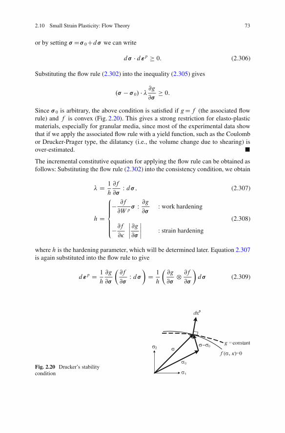
2.10 Small Strain Plasticity: Flow Theory 73
or by setting � D� 0Cd� we can write
d� � d"p 0: (2.306)
Substituting the flow rule (2.302) into the inequality (2.305) gives
.� � � 0/ � �@g
@� 0:
Since � 0 is arbitrary, the above condition is satisfied if gDf (the associated flowrule) and f is convex (Fig. 2.20). This gives a strong restriction for elasto-plasticmaterials, especially for granular media, since most of the experimental data showthat if we apply the associated flow rule with a yield function, such as the Coulombor Drucker-Prager type, the dilatancy (i.e., the volume change due to shearing) isover-estimated. �
The incremental constitutive equation for applying the flow rule can be obtained asfollows: Substituting the flow rule (2.302) into the consistency condition, we obtain
� D 1
h
@f
@�W d� ; (2.307)
h D
8ˆ<ˆ:
� @f
@W p� W @g
@�: work hardening
�@f
@�
ˇˇ @g
@�
ˇˇ : strain hardening
(2.308)
where h is the hardening parameter, which will be determined later. Equation 2.307is again substituted into the flow rule to give
d"p D 1
h
@g
@�
�@f
@�W d�
�D 1
h
�@g
@�˝ @f
@�
�d� (2.309)
Fig. 2.20 Drucker’s stabilitycondition

74 2 Introduction to Continuum Mechanics
where ˝ denotes the tensor product, and if @g=@� and @f =@� are represented asvectors, it becomes
@g
@�˝ @f
@�D
�@g
@�
�@f
@�
T
: (2.310)
Equation 2.309 can be written in the indicial notation:
d"pij D 1
h
@g
@�ij
@f
@�kld�kl: (2.311)
Let C p be the plastic compliance tensor (cf. (2.309)) given by
C p D 1
h
@g
@�˝ @f
@�or C
pij D 1
h
@g
@�ij
@f
@�kl; (2.312)
then we haved"p D C pd� or d"
pij D C
p
ijkld�kl: (2.313)
Equation 2.309 (or 2.313) is referred to as Melan’s formula.Since the plastic compliance tensor C p of (2.312), determined by the flow rule, is
represented by a product of two second-order tensors, the determinant is identicallyzero (det C p D0, if we set the second-order tensors as vectors as mentioned in(2.310)). Since it is not possible to obtain the inverse of C p directly, we use theproperties of the elastic compliance C e , which has the inverse, along with the directsum of the strain increment given by (2.293). That is,
d" D d"e C d"p D .C e C C p/ d� ;
) d� D Depd"; Dep D .C e C C p/�1 : (2.314)
Dep is determined explicitly as follows. Let
d� D Ded"e D De .d" � d"p/ D Ded" � De 1
h
@g
@�
�@f
@�W d�
�: (2.315)
Taking the inner-product with @f =@� , the above gives
@f
@�W d� D h
H
@f
@�W Ded"; H D h C @f
@�W�
De @g
@�
�: (2.316)
Using the symmetry property of De and substituting (2.316) into (2.315), we obtain
d� D Depd"; (2.317)
where
Dep D De � 1
H
�De @g
@�
�˝
�De @f
@�
�: (2.318)

2.10 Small Strain Plasticity: Flow Theory 75
The indicial form of Dep is given by
Dep
ijkl D Deijkl � 1
H
�De
ij mn
@g
@�mn
� �De
klst
@f
@�st
�: (2.319)
We now need to determine the hardening parameter h. For simplicity we use theisotropic hardening model (2.307), and from (2.308) we have
h D
8ˆ<ˆ:
@K
@W p� W @g
@�: work-hardening;
@K
@�
ˇˇ @g
@�
ˇˇ : strain-hardening:
(2.320)
A function �.x/ is said to be m-th order homogeneous of x if, for any scalar t ,
�.tx/ D tm�.x/:
Then we have the following Euler’s theorem (cf. Note 3.8, p. 108):
x � @�
@xD m �.x/
It should be noted that the von Mises .f1 DpJ2/ and Drucker-Prager .f1 Dp
J2 C˛I1/ yield functions are first order homogeneous functions; however
f1 D J2 C ˛I1
is not a homogeneous function.Let us apply the associated flow rule .gDf / and assume that f is an m-th order
homogeneous function, so that the work-hardening rule (2.320) can be written as
h D m@K
@W pf1: (2.321)
If we define the equivalent stress by
f1.� / D �e; (2.322)
and determine the equivalent plastic strain increment by
dW p D � W d"p � �e d"pe ; (2.323)
the hardening parameter can be specified by
h D m@�e
@"pe
: (2.324)

76 2 Introduction to Continuum Mechanics
Let us now consider the physical implications of the equivalent stress and strain. Formetallic materials, which show no volumetric plastic straining, we have
� W d"p D s dep C N�d N"p D s dep:
where dep is the deviatoric plastic strain increment and d N"p is the volumetricplastic strain increment, and therefore (2.323) is meaningful. However, for porousmaterials that show a considerable amount of volumetric plastic strain the conceptof equivalent stress and strain defined by (2.323) is not appropriate. Note that inthe metallic plasticity theory, in order to utilize the result of simple tension wesometimes define
�e Dp
3J2 .D �11/;
and introduce
d"pe D
r2
3dep W dep:
This, of course, causes an adjustment of the coefficients.

http://www.springer.com/978-3-642-25332-4