Nonlinear Continuum Mechanics · Nonlinear Continuum Mechanics Theory Manuals (9/22/98) Nonlinear Continuum Mechanics - Main Menu 1 < Go Back i Blue text ... deformation analysis

Nonlinear Continuum Mechanics

Theory Manuals (9/22/98) Nonlinear Continuum Mechanics - Main Menu 1

< Go Back

i

Blue textindicates

a link to moreinformation.

Formulation of Nonlinear Problems

Finite Element Formulations

SEACAS Library

Theory Manuals

Constitutive Models

SPH Formulation

Contact Surfaces


Introduction

Measures of Deformation

Rates of Deformation

Stress Measures

Balance Laws

Frame Indifference

Two-Dimensional Formulations

Structural Components

Rigid Bodies

Theory Manuals (9

< Go Back

Introduction Measures of Deformation


i

Blue textindicates



SEACAS Library

Theory Manuals

Stress Measures

Balance Laws

Frame Indifference

Two Dimensional Formulations

RigidBodies


Introduction

Overview

/22/98) Nonlinear Continuum Mechanics - Introduction 1

Theory Manuals (9

< Go Back

Introduction


SEACAS Library

Theory Manuals

gorous

n of

ontext. large to s. We hich

s tion

rk,

three

Overview

In this report we examine in detail the continuum mechanical issues necessary for rispecification of large deformation problems in solid mechanics. The discussion will provide a bridge between the generic problem statement given at the close of Formulation of Nonlinear Problems and the in-depth presentation of constitutive theory to be discussed in Constitutive Modeling. At the close of the latter report, we will be in a position to turn attention to numerical methods as applied to large deformation solidmechanics.

The current report’s presentation is organized as follows. We begin with a discussiolarge deformation kinematics, including consideration of velocity and acceleration measures and the quantification of deformation and deformation rates in a general cWe then discuss the various measures of stress that are frequently encountered in deformation analysis. With these preliminaries in hand, we will then be in a positionstate the relevant balance laws in notation appropriate for large deformation problemwill also at this point discuss the important concept of material frame indifference, wdemands that material laws be unaltered by rigid body motions. We will see that thiconcept places important restrictions on the kinematic and stress measures that aresuitable for prescription of constitutive laws, providing important background informafor a subsequent report.

The above information will be presented in a three-dimensional notational framewoassuming that the solids of interest are likewise fully three-dimensional continua. Formulations appropriate for two-dimensional problems and for structural entities in

/22/98) Nonlinear Continuum Mechanics - Introduction - Overview 2

Theory Manuals (9

< Go Back

Introduction


SEACAS Library

Theory Manuals

y tries

id

chapter

en

dimensions can be readily deduced from these equations. Accordingly, we will brieflpresent the modifications necessary to adapt our theory to two-dimensional geomeand to problems possessing axial symmetry. Also we will discuss how continuum mechanical descriptions of structural elements, including shells and beams, can bededuced from the three-dimensional formalism. We will also briefly examine how rigbodies can be incorporated into the notational structure we propose.

It should be emphasized that although many of the concepts to be discussed in this are applicable to Eulerian formulations, the presentation is targeted primarily towardLagrangian description of boundary value problems. Furthermore, for notational simplicity we work almost exclusively in Cartesian coordinate systems rather than ingeneral curvilinear coordinates (some deviation from this is obviously necessary whaxisymmetry is discussed). The interested reader may care to consult [Fung, Y.C., 1965] for discussion of such curvilinear formulations in a small-strain context, and [Marsden, J.E. and Hughes, T.J.R., 1983] for their rigorous extension to large deformation problems.

/22/98) Nonlinear Continuum Mechanics - Introduction - Overview 3

Theory Manuals (9

< Go Back


Introduction Rates of Deformation

i

Blue textindicates



SEACAS Library

Theory Manuals

Stress Measures

Balance Laws

Frame Indifference


RigidBodies




/22/98) Nonlinear Continuum Mechanics - Measures of Deformation 1

Theory Manuals (9

< Go Back



SEACAS Library

Theory Manuals

hich

r case indices inue to

tion at

f


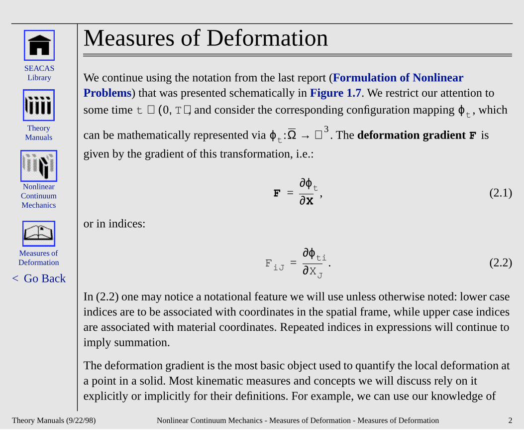
We continue using the notation from the last report (Formulation of Nonlinear Problems) that was presented schematically in Figure 1.7. We restrict our attention to

some time , and consider the corresponding configuration mapping , w

can be mathematically represented via . The deformation gradient is

given by the gradient of this transformation, i.e.:

, (2.1)

or in indices:

. (2.2)

In (2.2) one may notice a notational feature we will use unless otherwise noted: loweindices are to be associated with coordinates in the spatial frame, while upper case are associated with material coordinates. Repeated indices in expressions will contimply summation.

The deformation gradient is the most basic object used to quantify the local deformaa point in a solid. Most kinematic measures and concepts we will discuss rely on it explicitly or implicitly for their definitions. For example, we can use our knowledge o

t 0 T,( )∈ ϕ t

ϕ t :Ω ℜ 3→ F

FX∂

∂ϕ t=

FiJ XJ∂∂ϕ ti=

/22/98) Nonlinear Continuum Mechanics - Measures of Deformation - Measures of Deformation 2

Theory Manuals (9

< Go Back



SEACAS Library

Theory Manuals

be of d to be

f

ed to

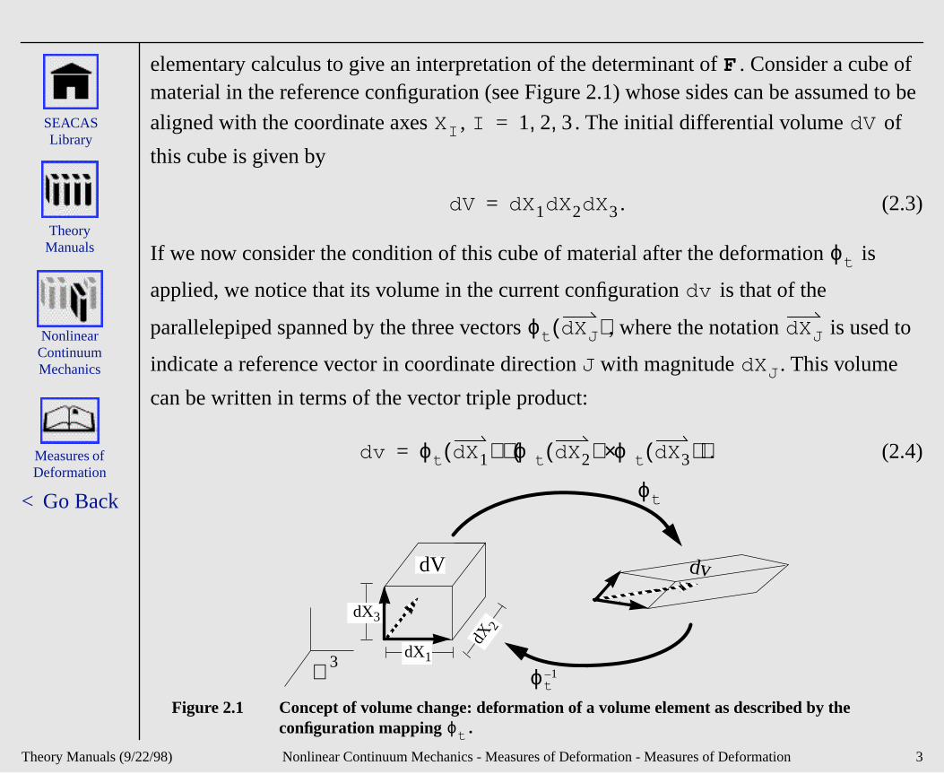
elementary calculus to give an interpretation of the determinant of . Consider a cumaterial in the reference configuration (see Figure 2.1) whose sides can be assume

aligned with the coordinate axes , . The initial differential volume o

this cube is given by

. (2.3)

If we now consider the condition of this cube of material after the deformation is

applied, we notice that its volume in the current configuration is that of the

parallelepiped spanned by the three vectors , where the notation is us

indicate a reference vector in coordinate direction J with magnitude . This volume

can be written in terms of the vector triple product:

. (2.4)

Figure 2.1 Concept of volume change: deformation of a volume element as described by the configuration mapping .

F

XI I 1 2 3, ,= Vd

Vd X1 X2 X3ddd=

ϕ t

vd

ϕ t XJd( ) XJd

XJd

vd ϕ t X1d( ) ϕ t X2d( ) ϕ t X3d( )×( )⋅=

ϕ t

dX2

dX1

dX3

dV

ℜ 3ϕ t

1–

dv

ϕ t


Theory Manuals (9

< Go Back



SEACAS Library

Theory Manuals

of

tor

de:

ors

If we consider any differential vector in the reference configuration, the calculus

differentials tells us that application of the mapping will produce a differential vec

whose coordinates are given via

. (2.5)

Application of this logic to the particular differential vectors leads one to conclu

. (2.6)

We can write (2.4) in indicial notation by first noting that the cross product of two vecta and b is written as

, (2.7)

where , the permutation symbol, has the following interpretation:

Rd

ϕ t

rd ϕ t Rd( )=

rd( )i XK∂∂ϕ ti Rd( )K=

XJd

ϕ t XJd( )( )i

Fi 1 X1d J = 1,

Fi 2 X2d J = 2,

Fi 3 X3d J = 3,

=

a b×( )i e ijk a j bk=

eijk


Theory Manuals (9

< Go Back



SEACAS Library

Theory Manuals

e

es

. For

ich

. (2.8)

Equation (2.4) is then reexpressed via

, (2.9)

where we have used Eq. (2.3) and the fact that (which can b

verified through actual trial). Introducing the notation , we conclude

. (2.10)

Equation (2.10) tells us that the deformation converts reference differential volum

to current volumes according to the determinant of the deformation gradient

this mapping to make physical sense, the current volume should be positive whthen places a physical restriction upon F that must be obeyed pointwise throughout themedium:

. (2.11)

eijk

1 if i j k, ,( ) = (1,2,3) or (2,3,1) or (3,1,2)

1– if i j k, ,( ) = (3,2,1) or (2,1,3) or (1,3,2)

0 otherwise

=

vd Fi 1 X1 eijk Fj 2 X2Fk3 X3dd( )d=

eijk Fi 1

Fj 2Fk3 X1 X2 X3ddd det F( ) Vd= =

det F( ) eijk Fi 1

Fj 2Fk 3=

J det F( )=

vd J Vd=

ϕ t

Vd vd

vd

J det F( ) detX∂

∂ϕ 0>= =


Theory Manuals (9

< Go Back



SEACAS Library

Theory Manuals

ing to ient e have

clude

an

ted the e

This physical restriction has important mathematical consequences as well. Accordthe inverse function theorem of multivariate calculus, a smooth function whose gradhas a nonzero determinant possesses a smooth and differentiable inverse. Since w

assumed to be smooth and physical restrictions demand that , we can con

that a function exists that is differentiable; in fact, the gradient of this function is

given by

. (2.12)

We will assume throughout the remainder of our discussion that , so that suchinverse is guaranteed to exist.

With the definition of F in hand, we turn our attention to the quantification of local deformation in a body. For any matrix, such as F, whose determinant is positive, the following decompositions can always be made:

. (2.13)

In (2.13) is a proper orthogonal tensor (right-handed rotation), while and arepositive definite and symmetric tensors. One can show that under the conditions stadecompositions in (2.13) can always be made and that, in fact, they are unique. Thinterested reader should consult [Gurtin, M.E., 1981], Chapter 1 for details. The decompositions in (2.13) are called right and left polar decompositions of F, respectively.

ϕ t J 0≠

ϕ t1–

x∂∂ϕ t

1–

F1–

=

J 0>

F RU VR= =

R U V


Theory Manuals (9

< Go Back



SEACAS Library

Theory Manuals

e right

oods ee

ting of

e nded)

,

en

se is

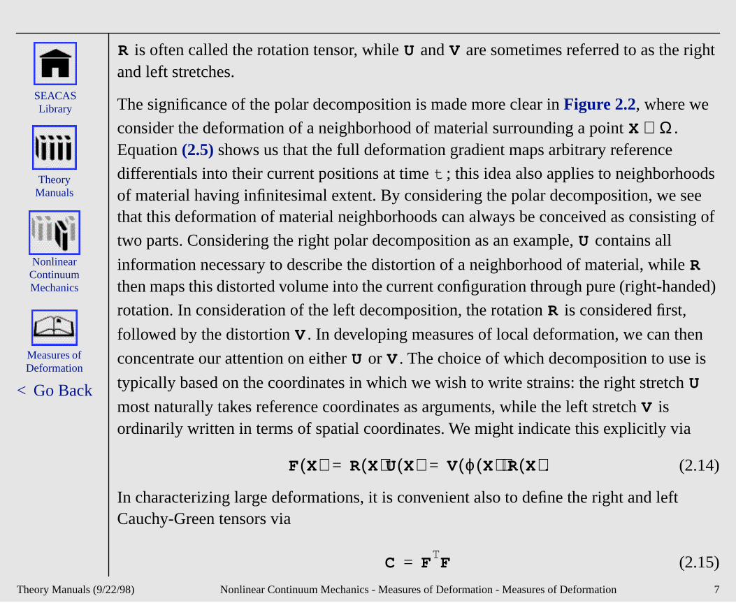
is often called the rotation tensor, while and are sometimes referred to as thand left stretches.

The significance of the polar decomposition is made more clear in Figure 2.2, where we

consider the deformation of a neighborhood of material surrounding a point . Equation (2.5) shows us that the full deformation gradient maps arbitrary reference

differentials into their current positions at time ; this idea also applies to neighborhof material having infinitesimal extent. By considering the polar decomposition, we sthat this deformation of material neighborhoods can always be conceived as consis

two parts. Considering the right polar decomposition as an example, contains all

information necessary to describe the distortion of a neighborhood of material, whilthen maps this distorted volume into the current configuration through pure (right-ha

rotation. In consideration of the left decomposition, the rotation is considered first

followed by the distortion . In developing measures of local deformation, we can th

concentrate our attention on either or . The choice of which decomposition to u

typically based on the coordinates in which we wish to write strains: the right stretch

most naturally takes reference coordinates as arguments, while the left stretch isordinarily written in terms of spatial coordinates. We might indicate this explicitly via

. (2.14)

In characterizing large deformations, it is convenient also to define the right and leftCauchy-Green tensors via

(2.15)

R U V

X Ω∈

t

U

R

R

V

U V

U

V

F X( ) R X( )U X( ) V ϕ X( )( )R X( )= =

C FTF=


Theory Manuals (9

< Go Back



SEACAS Library

Theory Manuals

and

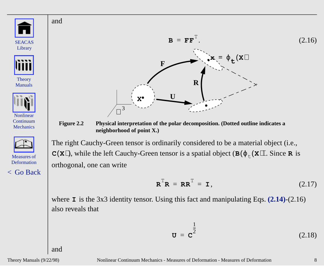
. (2.16)

Figure 2.2 Physical interpretation of the polar decomposition. (Dotted outline indicates a neighborhood of point X.)

The right Cauchy-Green tensor is ordinarily considered to be a material object (i.e.,

), while the left Cauchy-Green tensor is a spatial object ( . Since is

orthogonal, one can write

, (2.17)

where is the 3x3 identity tensor. Using this fact and manipulating Eqs. (2.14)-(2.16) also reveals that

(2.18)

and

B FFT

=

ℜ 3

R

U

F

X

x ϕt X( )=

C X( ) B ϕ t X( )( ) R

RTR RR

TI= =

I

U C

12---

=


Theory Manuals (9

< Go Back



SEACAS Library

Theory Manuals

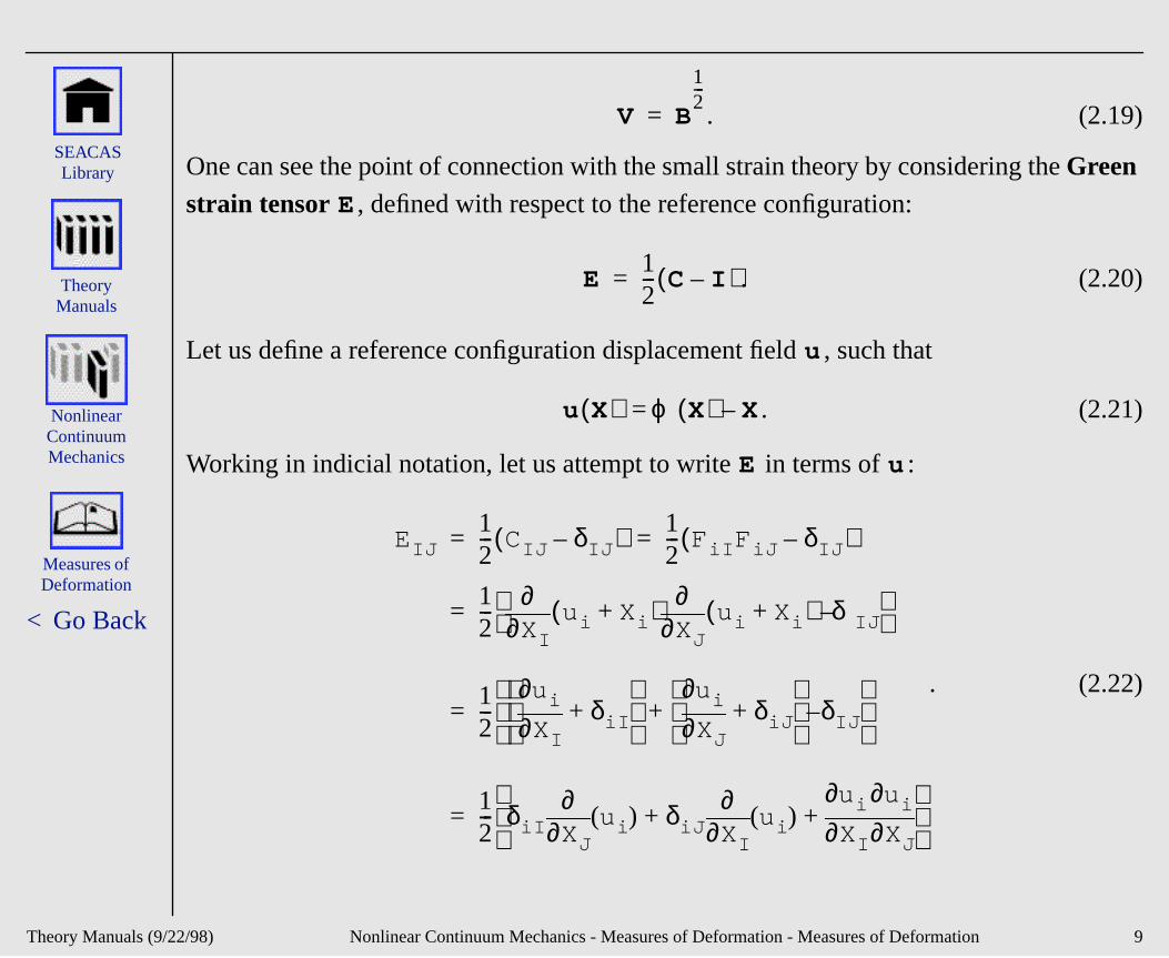
. (2.19)

One can see the point of connection with the small strain theory by considering the Green strain tensor , defined with respect to the reference configuration:

. (2.20)

Let us define a reference configuration displacement field , such that

. (2.21)

Working in indicial notation, let us attempt to write in terms of :

. (2.22)

V B

12---

=

E

E12--- C I–( )=

u

u X( ) ϕ X( ) X–=

E u

EIJ12--- CIJ δIJ–( ) 1

2--- FiI FiJ δIJ–( )= =

12---

XI∂∂

ui Xi+( )XJ∂∂

ui Xi+( ) δIJ– =

12---

XI∂∂ui δiI+

XJ∂∂ui δiJ+

δIJ–+

=

12--- δiI XJ∂

∂ui( ) δiJ XI∂

∂ui( )

XI∂∂ui

XJ∂∂ui+ +

=


Theory Manuals (9

< Go Back



SEACAS Library

Theory Manuals

c term

, in

size of

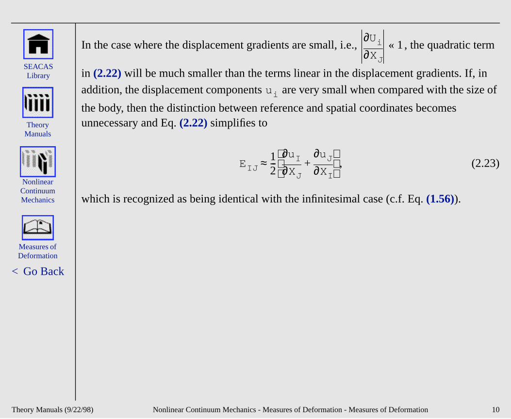
In the case where the displacement gradients are small, i.e., , the quadrati

in (2.22) will be much smaller than the terms linear in the displacement gradients. If

addition, the displacement components are very small when compared with the

the body, then the distinction between reference and spatial coordinates becomes unnecessary and Eq. (2.22) simplifies to

, (2.23)

which is recognized as being identical with the infinitesimal case (c.f. Eq. (1.56)).

XJ∂∂Ui 1«

ui

EIJ12---

XJ∂∂uI

XI∂∂uJ+

≈


Theory Manuals (9

< Go Back

Rates of Deforamtion


Introduction

i Blue textindicates



SEACAS Library

Theory Manuals

Stress Measures

Balance Laws

Frame Indifference


RigidBodies



Introduction

Material and Spatial Velocity and Acceleration

Rate of Deformation Tensors

/22/98) Nonlinear Continuum Mechanics - Rates of Deformation 1

Theory Manuals (9

< Go Back



SEACAS Library

Theory Manuals

es

w time

ere

Introduction

The development of the last section fixed our attention on an instant , andproposed some measurements of material deformation in terms of the configuration

mapping . We now allow time to vary and consider two questions: 1) how velociti

and accelerations are quantified in both the spatial and reference frames; and 2) hoderivatives of deformation measures are properly considered in a large deformationframework. The former topic is obviously crucial in the formulation of dynamics problems, while the latter is necessary, for example, in rate-dependent materials whquantities, such as strain rate, must be quantified.

t 0 T,( )∈

ϕ t

/22/98) Nonlinear Continuum Mechanics - Rates of Deformation - Introduction 2

Theory Manuals (9

< Go Back



SEACAS Library

Theory Manuals

rence s of

tten in

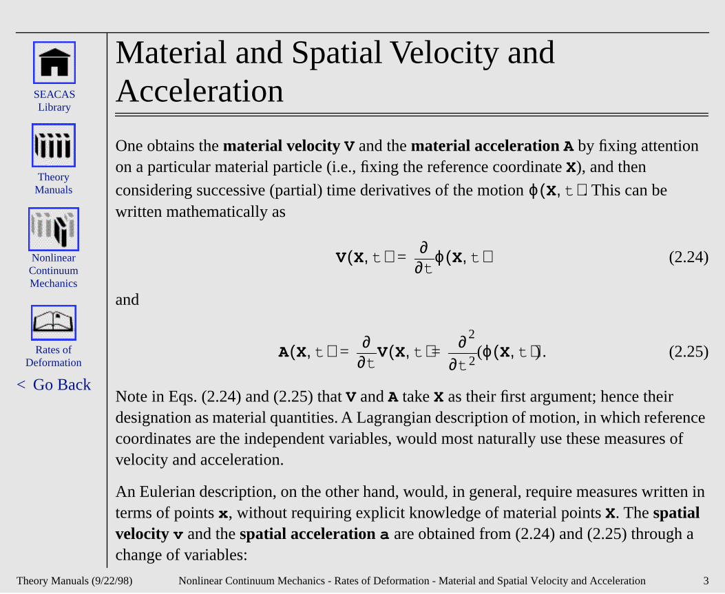
Material and Spatial Velocity and Acceleration

One obtains the material velocity V and the material acceleration A by fixing attention on a particular material particle (i.e., fixing the reference coordinate X), and then

considering successive (partial) time derivatives of the motion . This can be written mathematically as

(2.24)

and

. (2.25)

Note in Eqs. (2.24) and (2.25) that V and A take X as their first argument; hence their designation as material quantities. A Lagrangian description of motion, in which refecoordinates are the independent variables, would most naturally use these measurevelocity and acceleration.

An Eulerian description, on the other hand, would, in general, require measures writerms of points x , without requiring explicit knowledge of material points X. The spatial velocity v and the spatial acceleration a are obtained from (2.24) and (2.25) through achange of variables:

ϕ X t,( )

V X t,( )t∂∂ ϕ X t,( )=

A X t,( )t∂∂

V X t,( )t 2

2

∂∂= ϕ X t,( )( )=

/22/98) Nonlinear Continuum Mechanics - Rates of Deformation - Material and Spatial Velocity and Acceleration 3

Theory Manuals (9

< Go Back



SEACAS Library

Theory Manuals

e

tial his

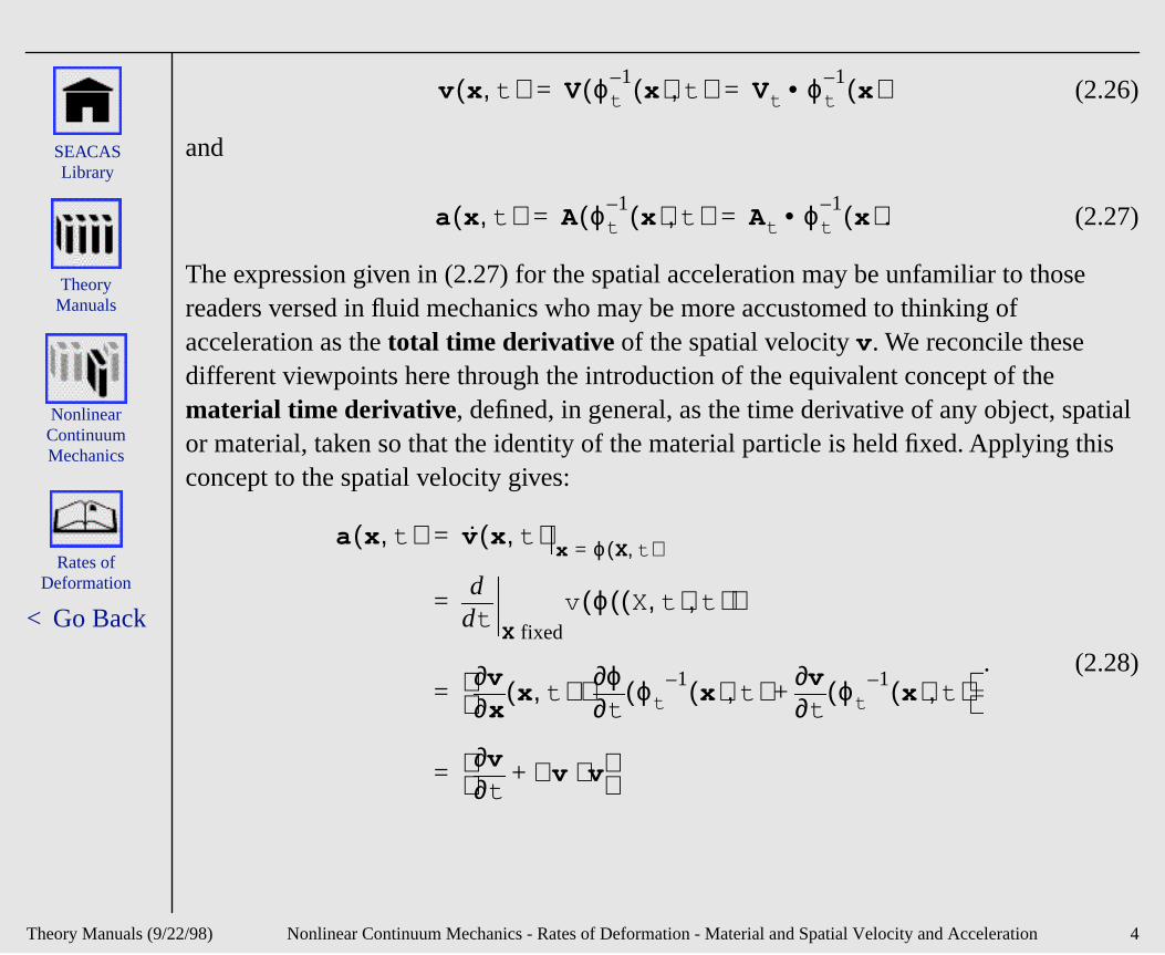
(2.26)

and

. (2.27)

The expression given in (2.27) for the spatial acceleration may be unfamiliar to thosreaders versed in fluid mechanics who may be more accustomed to thinking of acceleration as the total time derivative of the spatial velocity v . We reconcile these different viewpoints here through the introduction of the equivalent concept of the material time derivative, defined, in general, as the time derivative of any object, spaor material, taken so that the identity of the material particle is held fixed. Applying tconcept to the spatial velocity gives:

. (2.28)

v x t,( ) V ϕ t1–

x( ) t,( ) Vt ϕ t1–

x( )•= =

a x t,( ) A ϕ t1–

x( ) t,( ) At ϕ t1–• x( )= =

a x t,( ) v x t,( )x ϕ X t,( )=

=

tdd

X fixed

v ϕ X t,( ) t,( )( )=

x∂∂v

x t,( )t∂

∂ϕ ϕ t1–

x( ) t,( )⋅t∂

∂v ϕ t1–

x( ) t,( )+ =

t∂∂v

v∇ v⋅+ =


Theory Manuals (9

< Go Back



SEACAS Library

Theory Manuals

.

en in

plied he

e

This may be recognized as the so-called “total time derivative” of the spatial velocityExercising the concept of a material time derivative a little further, we can see from (2.24) that the material velocity is the material time derivative of the motion, so that

. (2.29)

Comparing Eqs. (2.25) and (2.28), we can also conclude that A and a are, in fact, the samephysical entity expressed in different coordinates. The former is most naturally writtterms of V, while the latter is conveniently expressed in terms of v .

One may see in (2.28) the superposed dot notation for the time derivative of . Such superposed dots will always imply a material time derivative in this text, whether apto material quantities or, as in this case, spatial ones. It is further emphasized that t

gradient is taken with respect to spatial coordinates and is, therefore, called thespatial velocity gradient. It is used often enough to warrant a special symbol which wdenote as L:

. (2.30)

v

V ϕ=

v

∇ v

L v∇=


Theory Manuals (9

< Go Back



SEACAS Library

Theory Manuals

,

ure of

ate of .31) fined rparts f the r

Rate of Deformation Tensors

From the spatial gradient L defined in (2.30), we can define two spatial tensors and known respectively as the spatial rate of deformation tensor and the spatial spin tensor:

, (2.31)

and

. (2.32)

It is clear that is merely the symmetric part of the velocity gradient, while is theantisymmetric, or skew, portion.

The quantities and are spatial measures of deformation. is effectively a meas

strain rate suitable for large deformations, while provides a local measure of the rrotation of the material. In fact, it is readily verified that in small deformations, Eq. (2amounts to nothing more that the time derivative of the infinitesimal strain tensor dein (1.56). It is of interest at this point to discuss whether appropriate material counteof these objects exist. Toward this end let us calculate the material time derivative odeformation gradient F, noting in so doing that if F is an analytic function, then the ordeof partial differentiation can be reversed:

D W

D ∇ sv12--- L L

T+[ ]= =

W ∇ av12---= L L

T–[ ]=

D W

D W D

W

/22/98) Nonlinear Continuum Mechanics - Rates of Deformation - Rate of Deformation Tensors 6

Theory Manuals (9

< Go Back



SEACAS Library

Theory Manuals

e

. (2.33)

From (2.33) we conclude that the material time derivative is nothing more than thmaterial velocity gradient. Manipulating this quantity further we find

. (2.34)

Examination of (2.33) and (2.34) reveals that

. (2.35)

Recalling the definition for the right Cauchy-Green strain tensor C in Eq. (2.15), we compute its material time derivative via:

, (2.36)

which in view of (2.31), leads us to conclude

. (2.37)

Ft∂∂

X∂∂ ϕ X t,( )

X∂∂

t∂∂ ϕ X t,( )

X∂∂V= = =

F

X∂∂V

X∂∂

v °ϕ t( ) v∇ ϕ t X( )( )X∂∂ ϕ t X( )( )= =

L ϕ t X( )( )F X( )=

L F°ϕ t1–( )F 1–

=

Ct∂∂

FTF[ ] FTF FTF+= =

LF( )TF FT LF( )+ FT L LT

+( )F= =

C X t,( ) 2FT X t,( )D ϕ t X( ) t,( )F X t,( )=


Theory Manuals (9

< Go Back



SEACAS Library

Theory Manuals

n

f our text is spect

as the by

n of

r.

In view of (2.37) is sometimes called the material rate of deformation tensor.

Noting that is the Jacobian of the transformation , readers with a background i

differential geometry will recognize as the pull-back of the spatial tensor field

defined on . Conversely, is the push-forward of the material tensor field

defined on . The concepts of pull-back and push-forward are outside the scope opresent investigation, but the basic physical principle they embody in the current conperhaps useful. Loosely speaking, the push-forward (or pull-back) of a tensor with reto a given transformation produces a tensor in the new frame of reference that we, observers, would observe as identical to the original tensor if we were embedded inmaterial during the transformation. Thus the same physical principle is represented

both and , but they are very different objects mathematically since the

transformation that interrelates them is the deformation itself. Recalling the definitio

Green’s strain given in Eq. (2.20), we can easily see that

. (2.38)

This further substantiates the interpretation of as a strain rate as suggested earlie

12---C

F ϕ t

12---C D

ϕ t Ω( ) D12---C

Ω

12---C D

E

E12---C FTDF= =

D


Theory Manuals (9

< Go Back



SEACAS Library

Theory Manuals

the

for the

ck

lating

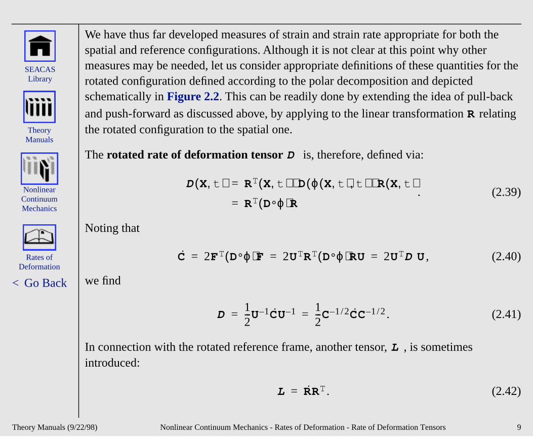
We have thus far developed measures of strain and strain rate appropriate for both spatial and reference configurations. Although it is not clear at this point why other measures may be needed, let us consider appropriate definitions of these quantitiesrotated configuration defined according to the polar decomposition and depicted schematically in Figure 2.2. This can be readily done by extending the idea of pull-ba

and push-forward as discussed above, by applying to the linear transformation rethe rotated configuration to the spatial one.

The rotated rate of deformation tensor is, therefore, defined via:

. (2.39)

Noting that

, (2.40)

we find

. (2.41)

In connection with the rotated reference frame, another tensor, , is sometimes introduced:

. (2.42)

R

D

D X t,( ) RT X t,( ) D ϕ X t,( ) t,( ) R X t,( )⋅ ⋅=

RT D°ϕ( )R=

C 2FT D°ϕ( )F 2UTRT D°ϕ( )RU 2UTD U= = =

D12---U 1– CU 1– 1

2---C 1 2/– CC 1 2/–= =

L

L RRT=


Theory Manuals (9

< Go Back



SEACAS Library

Theory Manuals

d ence.

As shown below, note that is skew:

. (2.43)

We will return later in this report to the various measures associated with the rotateconfiguration. They have particular importance in the study of material frame indiffer

L

L L T+ RRT RRT+t∂∂

RRT( )t∂

∂I 0= = = =


Theory Manuals (9

< Go Back

Stress Measures






SEACAS Library

Theory Manuals

Introduction Balance Laws

Frame Indifference


RigidBodies


Stress Measures

Stress Measures

/22/98) Nonlinear Continuum Mechanics - Stress Measures 1

Theory Manuals (9

< Go Back

Stress Measures


SEACAS Library

Theory Manuals

y ss , this

n at a

rms of

ay

h the

Stress Measures

In this section we discuss the quantification of force intensity, or stress, within a bodundergoing potentially large amounts of deformation. We begin with the Cauchy stretensor T, and note that provided we associate this object with the spatial configurationobject can be interpreted exactly as in the infinitesimal case outlined in Linear Elastic IBVP . In the current notational framework, we interpret the components of T, which we

shall denote as , as representing forces per unit areas in the spatial configuratio

given spatial point .

It will be necessary in our study to consider related measures of stress defined in tethe other configurations we have discussed, particularly the reference and rotated configurations. To motivate this discussion, let us reconsider the concept of tractiondiscussed previously in the context of the infinitesimal elastic system. The reader mrecall that given a plane passing through the point of interest x , the traction, or force per unit area acting on this plane, is given by the formula

, (2.44)

where is the unit normal vector to the plane in question.

Let us consider two differential vectors, and , in such a plane passing throug

spatial point x , as indicated in Figure 2.3. We assume that and are linearly

independent from one another and that both differential vectors have x as their base point.

Tij

x ϕ t Ω( )∈

t i Tij n j=

nj

r 1d r 2d

r 1d r 2d

/22/98) Nonlinear Continuum Mechanics - Stress Measures - Stress Measures 2

Theory Manuals (9

< Go Back

Stress Measures


SEACAS Library

Theory Manuals

asic

.

ctors

two

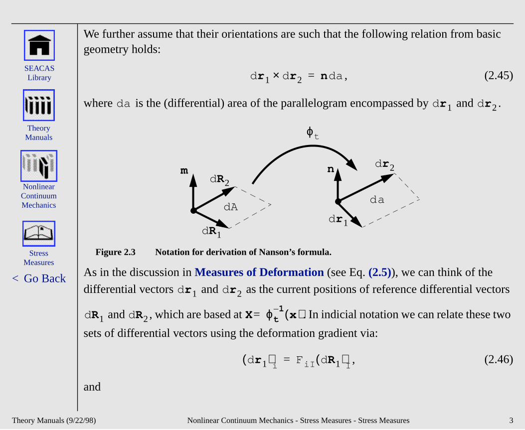
We further assume that their orientations are such that the following relation from bgeometry holds:

, (2.45)

where is the (differential) area of the parallelogram encompassed by and

Figure 2.3 Notation for derivation of Nanson’s formula.

As in the discussion in Measures of Deformation (see Eq. (2.5)), we can think of the

differential vectors and as the current positions of reference differential ve

and , which are based at . In indicial notation we can relate these

sets of differential vectors using the deformation gradient via:

, (2.46)

and

r 1d r 2d× n ad=

ad r 1d r 2d

R1d

R2dm

Ad

ϕ t

da

n

r 1d

r 2d

r 1d r 2d

R1d R2d X ϕ= t1–

x( )

r 1d( )i

FiI R1d( )I

=


Theory Manuals (9

< Go Back

Stress Measures


SEACAS Library

Theory Manuals

y

. (2.47)

We now seek to reexpress (2.45) in terms of reference quantities. Working in indicial notation we can write

. (2.48)

Let us extract and work with a particular product in the last line of Eq. (2.48), namel

. One can show by a case-by-case examination that the following

relation holds:

. (2.49)

The reader may recall from Measures of Deformation that has the followingrepresentation in indicial notation:

. (2.50)

Combination of Eqs. (2.48), (2.49), and (2.50) yields the following result:

. (2.51)

r 2d( )i

FiI R2d( )I

=

ni ad e ijk FjJ R1d( )JFkK R2d( )

K=

eljk δli FjJ R1d( )JFkK R2d( )

K=

eljk FlL FLi1–

FjJ R1d( )JFkK R2d( )

K=

eljk FlL FjJ FkK

eljk FlL FjJ FkK eLJKeljk Fl 1Fj 2Fk3=

J det F( )=

J det F( ) eljk Fl 1Fj 2Fk 3= =

ni ad Je LJKFLi1–

R1d( )J

R2d( )K

=

JF Li1–

mL Ad=


Theory Manuals (9

< Go Back

Stress Measures


SEACAS Library

Theory Manuals

ong surface

ore

tress

In Eq. (2.51) is the differential reference area spanned by and , and m is the

reference unit normal to this area.

In direct notation we can express this result as

. (2.52)

Equation (2.52) is sometimes referred to as Nanson’s formula and it is important, amother reasons, because it provides the appropriate change-of-variables formula for integrals in the reference and current configurations. In the current context we are minterested in computing the product of the traction acting on our plane at x and the differential area under consideration. Denoting this differential force by df , we may write

. (2.53)

In examining (2.53) we find that the following definition is useful

, (2.54)

which then allows us to write

. (2.55)

In examining Eq. (2.55), we note that the product represents a traction, with thephysical interpretation of current force divided by reference area. The stress P is called the

(First ) Piola-Kirchhoff Stress, and like the associated Piola traction, , measures sby referencing the force acting on areas to the magnitude of those areas in their

Ad R1d R2d

n ad J FT–m Ad=

fd t ad Tn ad J TFT–m Ad= = =

P X( ) J X( )T ϕ t X( )( )F T– ϕ t X( )( )=

fd Pm Ad=

Pm

Pm


Theory Manuals (9

< Go Back

Stress Measures


SEACAS Library

Theory Manuals

ure is

g a

t.

tated

:

t

undeformed configurations. The one-dimensional manifestation of this stress meas

the engineering stress, , originally defined in Eq. (1.3).

in the sense discussed in Rates of Deformation, it is worthy to note that P is neither a pure spatial nor a reference object. Such an object can be constructed by performinpull-back of the spatial Cauchy stress tensor T to the reference configuration:

. (2.56)

is called the Second Piola-Kirchhoff stress tensor and it is a purely reference objec

We note in particular that is a symmetric tensor, while P is not symmetric, in general.

This same concept of pull-back can be employed to define a stress tensor in the ro

configuration, which we shall denote as . This rotated stress tensor is defined via

. (2.57)

As was the case with the rotated configuration quantities introduced in Rate of Deformation Tensors, this definition will be of particular importance in the subsequenexamination of frame indifference.

σE

S X( ) J F 1– ϕ t X( )( )T ϕ t X( )( )F T– ϕ t X( )( )=

F 1– ϕ t X( )( )P X( )=

S

S

T

T ϕ t X( )( ) RT ϕ t X( )( )T ϕ t X( )( )R ϕ t X( )( )=


Theory Manuals (9

< Go Back

Balance Laws






SEACAS Library

Theory Manuals

Stress Measures

Introduction Frame Indifference


RigidBodies


Balance Laws

Introduction

Localization

Conservation of Mass

Conservation of Linear Momentum

Conservation of Angular Momentum

Stress Power

/22/98) Nonlinear Continuum Mechanics - Balance Laws 1

Theory Manuals (9

< Go Back

Balance Laws


SEACAS Library

Theory Manuals

ressed . To can be

Introduction

In this section we examine the local forms of the various conservations laws as expin the various reference frames (spatial, reference, and rotated) we have introducedexpedite our development, we first discuss how integral representations of balancesconverted to pointwise conservation principles, a process known as localization.

/22/98) Nonlinear Continuum Mechanics - Balance Laws - Introduction 2

Theory Manuals (9

< Go Back

Balance Laws


SEACAS Library

Theory Manuals

ver all

e

other

in

Localization

Suppose we consider an arbitrary volume of material, , in the reference configuration of a solid body, as depicted in Figure 2.4. Suppose further that we can establish the following generic integral relation over this volume:

, (2.58)

where is some reference function, be it scalar, vector, or tensor-valued, defined o

of . Suppose now that (2.58) holds true for each and every subvolume of . Thlocalization theorem then states that

. (2.59)

The interested reader should consult [Gurtin, M.E., 1981], Section 5 for elaboration on this principle. It should be noted that the same procedure can be applied spatially. In

words, if we are working with a spatial object, we might consider arbitrary volumes

the spatial domain, and if the following holds for a spatial object for all :

, (2.60)

then throughout .

V Ω⊂

f X( ) VdV∫ 0=

f

Ω V Ω

f 0 pointwise in Ω=

v

g v

g x( ) vdv∫ 0=

g x( ) 0= ϕ t Ω( )

/22/98) Nonlinear Continuum Mechanics - Balance Laws - Localization 3

Theory Manuals (9

< Go Back

Balance Laws


SEACAS Library

Theory Manuals

alid
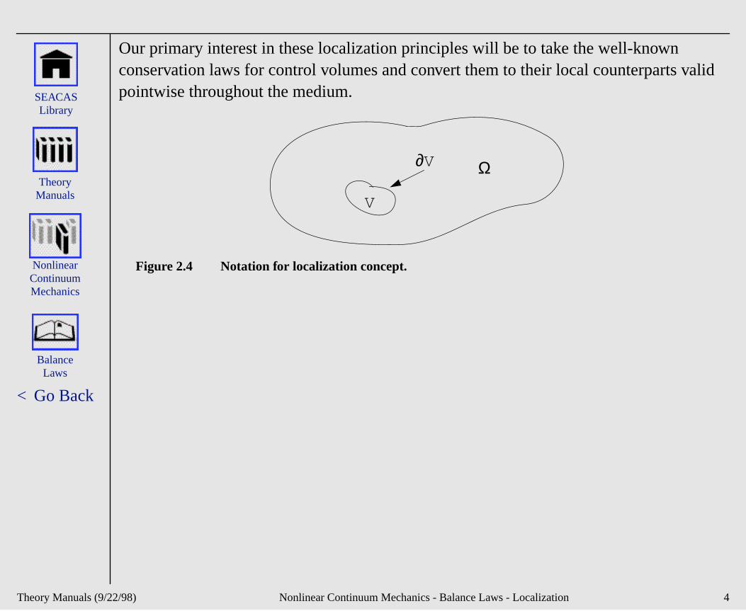
Our primary interest in these localization principles will be to take the well-known conservation laws for control volumes and convert them to their local counterparts vpointwise throughout the medium.
Figure 2.4 Notation for localization concept.

Ω

V

V∂

/22/98) Nonlinear Continuum Mechanics - Balance Laws - Localization 4

Theory Manuals (9

< Go Back

Balance Laws


SEACAS Library

Theory Manuals

, , in the via

lume,

n ed in

Conservation of Mass

In consideration of the conservation of mass, let us consider a fixed control volumethe spatial domain, completely filled with our solid body at the instant in question asbody moves through it. We may write a conservation of mass for this control volume

, (2.61)

where the term on the left can be interpreted as the net mass influx to the control voand the right-hand side is the rate of mass accumulation inside the control volume. Applying the divergence theorem to the left-hand side gives

. (2.62)

This can be further rearranged to yield

, (2.63)

which can be established for any arbitrary spatial volume . Applying the localizatiotheorem gives the local expression of continuity, which may be familiar to those versfluid mechanics:

v

ρv n ad⋅v∂∫–

t∂∂ρ

vdv∫=

∇ ρ v( ) vd⋅v∫–

t∂∂ρ

vdv∫=

t∂∂ρ ∇ρ v ρ ∇ v⋅( )+⋅+

vdv∫ 0=

v

/22/98) Nonlinear Continuum Mechanics - Balance Laws - Conservation of Mass 5

Theory Manuals (9

< Go Back

Balance Laws


SEACAS Library

Theory Manuals

cially

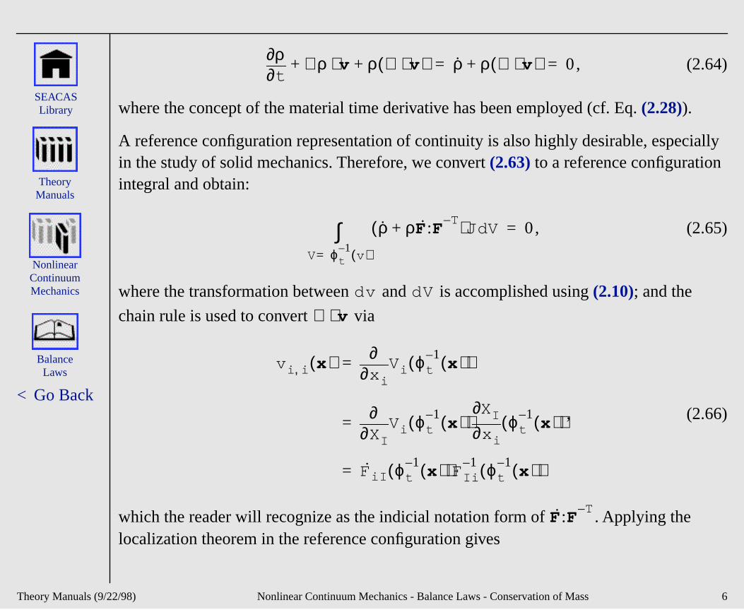
, (2.64)

where the concept of the material time derivative has been employed (cf. Eq. (2.28)).

A reference configuration representation of continuity is also highly desirable, espein the study of solid mechanics. Therefore, we convert (2.63) to a reference configurationintegral and obtain:

, (2.65)

where the transformation between and is accomplished using (2.10); and the

chain rule is used to convert via

, (2.66)

which the reader will recognize as the indicial notation form of . Applying the localization theorem in the reference configuration gives

t∂∂ρ ∇ρ v ρ ∇ v⋅( )+⋅+ ρ ρ ∇ v⋅( )+ 0= =

ρ ρF:FT–

+( )J Vd

V ϕ= t1–

v( )∫ 0=

dv dV

∇ v⋅

v i i, x( )x i∂∂

Vi ϕ t1–

x( )( )=

XI∂∂

Vi ϕ t1–

x( )( )x i∂

∂XI ϕ t1–

x( )( )=

FiI ϕ t1–

x( )( )FIi1– ϕ t

1–x( )( )=

F:FT–


Theory Manuals (9

< Go Back

Balance Laws


SEACAS Library

Theory Manuals

n

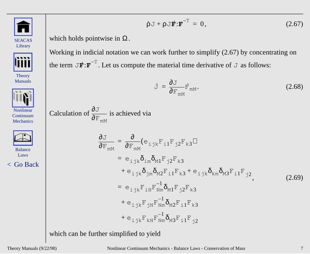
, (2.67)

which holds pointwise in .

Working in indicial notation we can work further to simplify (2.67) by concentrating o

the term . Let us compute the material time derivative of as follows:

. (2.68)

Calculation of is achieved via

, (2.69)

which can be further simplified to yield

ρJ ρJ F:FT–

+ 0=

Ω

J F:FT–

J

JFmM∂

∂JFmM=

FmM∂∂J

FmM∂∂J

FmM∂∂

eijk Fi 1Fj 2Fk3( )=

eijk δim δM1Fj 2Fk 3=

eijk δjm δM2Fi 1Fk 3 eijk δkmδM3Fi 1Fj 2

+ +

eijk FiN FNm1– δM1Fj 2Fk3=

eijk FjN FNm1– δM2Fi 1Fk3+

eijk FkNFNm1– δM3Fi 1F

j 2+


Theory Manuals (9

< Go Back

Balance Laws


SEACAS Library

Theory Manuals

tells ariant a

ed via

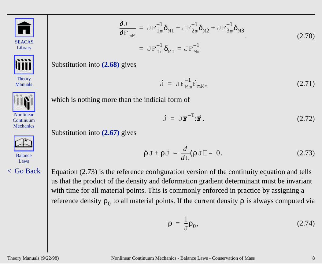
. (2.70)

Substitution into (2.68) gives

, (2.71)

which is nothing more than the indicial form of

. (2.72)

Substitution into (2.67) gives

. (2.73)

Equation (2.73) is the reference configuration version of the continuity equation andus that the product of the density and deformation gradient determinant must be invwith time for all material points. This is commonly enforced in practice by assigning

reference density to all material points. If the current density is always comput

, (2.74)

FmM∂∂J

JF 1m1– δM1 JF 2m

1– δM2 JF 3m1– δM3+ +=

JF Im1– δMI JF Mm

1–==

J JF Mm1–

FmM=

J J FT–:F=

ρJ ρJ+tdd ρJ( ) 0= =

ρ0 ρ

ρ 1J---ρ0=


Theory Manuals (9

< Go Back

Balance Laws


SEACAS Library

Theory Manuals

then Eq. (2.73) is automatically satisfied (recall that the Jacobian is unity in the reference configuration).

J


Theory Manuals (9

< Go Back

Balance Laws


SEACAS Library

Theory Manuals

ar

nts the duced

and

Conservation of Linear Momentum

Considering once more a fixed control volume , the control volume balance of linemomentum can be expressed as

. (2.75)

The first term on the left expresses the momentum outflux, while the second represerate of accumulation inside the control volume. This net change of momentum is pro

by the total resultant force on the system, equal to the sum effect of the body force

the surface tractions .

Applying the divergence theorem to both surface integrals, we find

, (2.76)

and

. (2.77)

Substituting (2.76) and (2.77) into (2.75) and rearranging gives

v

ρv( )v n ad⋅v∂∫ t∂

∂ ρv( ) vdv∫+ f v t ad

v∂∫+d

v∫=

F

t

ρv( )v n ad⋅v∂∫ ∇ ρ v( )v ρ ∇ v( )v+⋅[ ] vd

v∫=

t adv∂∫ Tn ad

v∂∫ ∇ T⋅ vd

v∫= =

/22/98) Nonlinear Continuum Mechanics - Balance Laws - Conservation of Linear Momentum 10

Theory Manuals (9

< Go Back

Balance Laws


SEACAS Library

Theory Manuals

utilized

rm of

. (2.78)

Employing the spatial form of the continuity equation (Eq.(2.63)) and recalling the formula for the material time derivative (Eq. (2.28)) gives

. (2.79)

By the localization theorem this implies

(2.80)

pointwise, which is recognized as the same statement of linear momentum balance in our earlier treatment of linear elasticity.

In large deformation problems it is desirable to also have a reference configuration fo(2.80). Converting (2.79) to its indicial form we have

. (2.81)

Working with the stress divergence term first we write

∇ T⋅ f ρt∂

∂v– ρ ∇ v( )v–+

t∂∂ρ

v– ∇ρ v⋅( )v– ρ ∇ v⋅( )v–

vdv∫ 0=

∇ T⋅ f ρv–+[ ] vdv∫ 0=

∇ T⋅ f ρ= v+

Tij j, f i ρv i–+[ ] vdv∫ 0=


Theory Manuals (9

< Go Back

Balance Laws


SEACAS Library

Theory Manuals

fact

. (2.82)

Using Eq. (2.54) we can write

. (2.83)

Using Eq. (2.70) we can simplify (2.83) and postmultiply by to obtain:

. (2.84)

The first and last terms on the right-hand side of (2.84) cancel each other due to the

that . Therefore, we have

. (2.85)

Using this result and applying a change of variables to (2.81) gives

Tij j, XJ∂∂Tij

x j∂∂XJ

XJ∂∂Tij

˙FJj

1–= =

XJ∂∂Tij

XJ∂∂ 1

J---PiI FjI

=

1–

J2

------FkK∂

∂JXJ∂

∂FkKPiI FjI1J---

XJ∂∂

PiI FjI( )+=

FJj1–

XJ∂∂Tij FJj

1– 1–J------FKk

1–

XJ∂∂FkKPiJ

1J---

XI∂∂PiI 1

J---FJj

1–

XJ∂∂FjI PiI+ +=

XJ∂∂FjI

XI∂∂FjJ=

XJ∂∂Tij FJj

1– 1J---

XI∂∂PiI=


Theory Manuals (9

< Go Back

Balance Laws


SEACAS Library

Theory Manuals

the

nce

erator

, (2.86)

where , the prescribed body force per unit reference volume. Employing

localization theorem gives

(2.87)

pointwise in , which expresses the balance of linear momentum in terms of refere

coordinates. In (2.87) we have used the notation to indicate the divergence opapplied in reference coordinates.

PiI I, Fi ρ0Vi–+( ) VdV∫ 0=

Fi Jf i=

DIV P F+ ρ0V=

ΩDIV


Theory Manuals (9

< Go Back

Balance Laws


SEACAS Library

Theory Manuals

e its

the

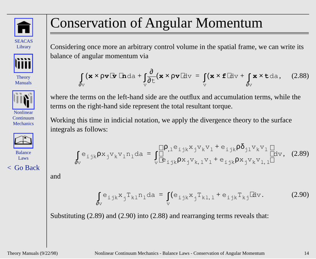
Conservation of Angular Momentum

Considering once more an arbitrary control volume in the spatial frame, we can writbalance of angular momentum via

, (2.88)

where the terms on the left-hand side are the outflux and accumulation terms, whileterms on the right-hand side represent the total resultant torque.

Working this time in indicial notation, we apply the divergence theory to the surface integrals as follows:

, (2.89)

and

. (2.90)

Substituting (2.89) and (2.90) into (2.88) and rearranging terms reveals that:

x ρv×( )v n ad⋅v∂∫ t∂

∂x ρv×( ) vd

v∫+ x f×( ) v x t× ad

v∂∫+d

v∫=

eijk ρx j v kv l n l adv∂∫

ρ,l e ijk x j v kv l e ijk+ ρδjl v kv l

e ijk ρx j v k l, v l e ijk ρx j v kv l l,+

vdv∫=

eijk xjTkl n l ad

v∂∫ eijk x

jTkl l, eijk Tkj+( ) vd

v∫=

/22/98) Nonlinear Continuum Mechanics - Balance Laws - Conservation of Angular Momentum 14

Theory Manuals (9

< Go Back

Balance Laws


SEACAS Library

Theory Manuals

f the

e ct, a frame.

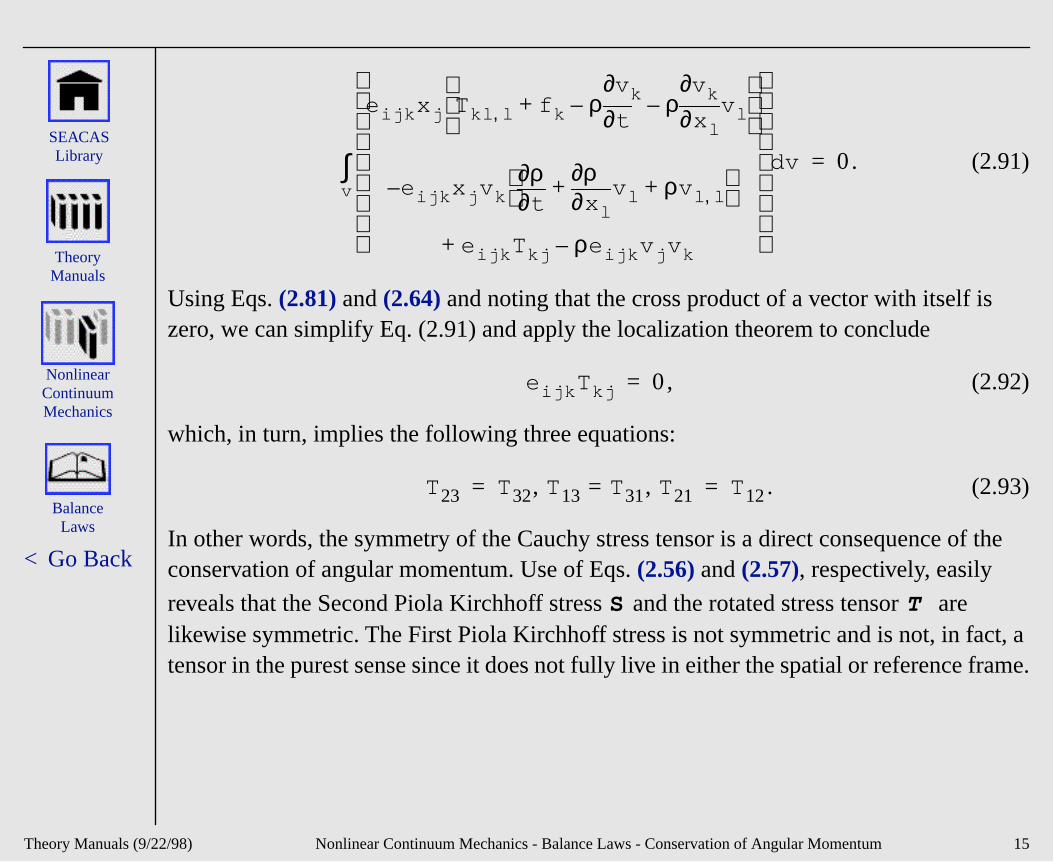
. (2.91)

Using Eqs. (2.81) and (2.64) and noting that the cross product of a vector with itself iszero, we can simplify Eq. (2.91) and apply the localization theorem to conclude

, (2.92)

which, in turn, implies the following three equations:

. (2.93)

In other words, the symmetry of the Cauchy stress tensor is a direct consequence oconservation of angular momentum. Use of Eqs. (2.56) and (2.57), respectively, easily

reveals that the Second Piola Kirchhoff stress and the rotated stress tensor arlikewise symmetric. The First Piola Kirchhoff stress is not symmetric and is not, in fatensor in the purest sense since it does not fully live in either the spatial or reference

eijk x j Tkl l, f k ρt∂

∂v k– ρx l∂

∂v k–+ v l

eijk x j v k t∂∂ρ

x l∂∂ρ

v l ρv l l,+ + –

eijk Tkj ρeijk v j v k–+

vdv∫ 0=

eijk Tkj 0=

T23 T32, T13 T31, T21= T12= =

S T

/22/98) Nonlinear Continuum Mechanics - Balance Laws - Conservation of Angular Momentum 15

Theory Manuals (9

< Go Back

Balance Laws


SEACAS Library

Theory Manuals

lance. e is no n other

s

als:

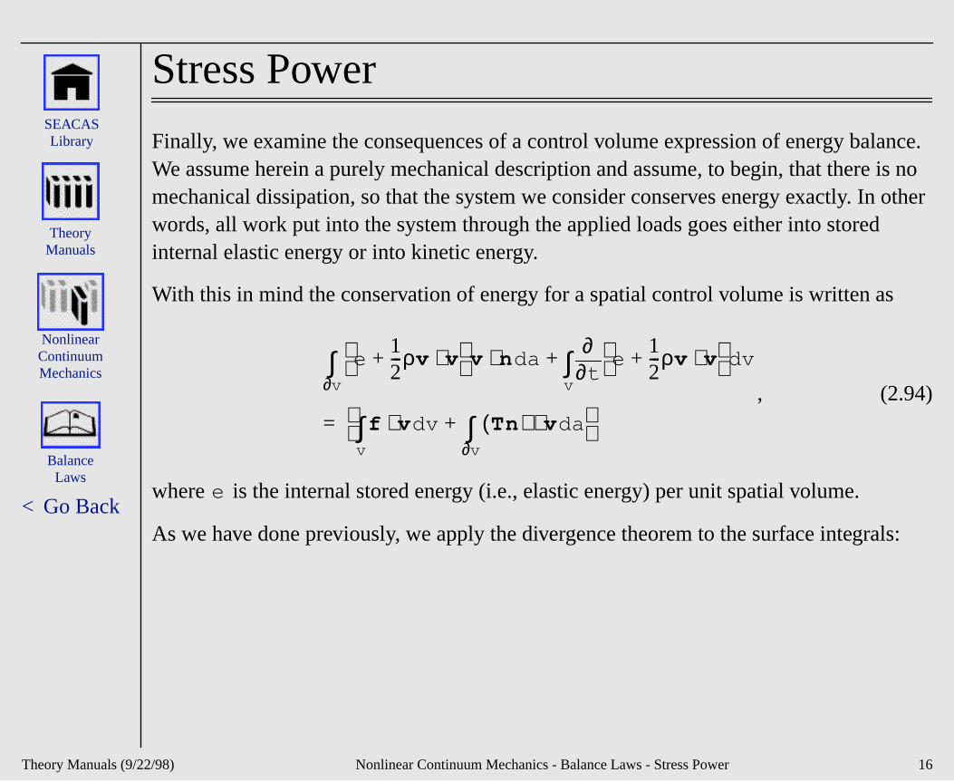
Stress Power

Finally, we examine the consequences of a control volume expression of energy baWe assume herein a purely mechanical description and assume, to begin, that thermechanical dissipation, so that the system we consider conserves energy exactly. Iwords, all work put into the system through the applied loads goes either into storedinternal elastic energy or into kinetic energy.

With this in mind the conservation of energy for a spatial control volume is written a

, (2.94)

where is the internal stored energy (i.e., elastic energy) per unit spatial volume.

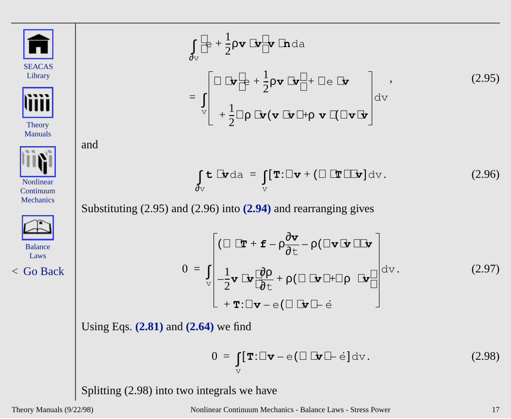
As we have done previously, we apply the divergence theorem to the surface integr

e12---ρv v⋅+

v n at∂∂

e12---ρv v⋅+

vdv∫+d⋅

v∂∫

fv∫ v vd⋅ Tn( ) v ad⋅

v∂∫+

=

e

/22/98) Nonlinear Continuum Mechanics - Balance Laws - Stress Power 16

Theory Manuals (9

< Go Back

Balance Laws


SEACAS Library

Theory Manuals

, (2.95)

and

. (2.96)

Substituting (2.95) and (2.96) into (2.94) and rearranging gives

. (2.97)

Using Eqs. (2.81) and (2.64) we find

. (2.98)

Splitting (2.98) into two integrals we have

e12---ρv v⋅+

v n ad⋅v∂∫

∇ v e12---ρv v⋅+

∇ e v⋅+⋅

12--- ∇ρ v v v⋅( ) ρv ∇ v( )v⋅+⋅+

vdv∫=

t v ad⋅v∂∫ T:∇ v ∇ T⋅( ) v⋅+[ ] vd

v∫=

0

∇( T f ρt∂

∂v– ρ ∇ v( )v )–+⋅ v⋅

12---v v

t∂∂ρ ρ ∇ v⋅( ) ∇ρ v⋅+ +

⋅–

T:∇ v e ∇ v⋅( )– e–+

vdv∫=

0 T:∇ v e ∇ v⋅( )– e–[ ] vdv∫=


Theory Manuals (9

< Go Back

Balance Laws


SEACAS Library

Theory Manuals

In so usly to

nt

. (2.99)

We now wish to convert (2.99) to the reference configuration and apply localization.doing we recognize that the second integral in (2.99) can be treated directly analogo

that of Eq. (2.63), with the density in (2.63) being replaced by the energy in the currecase. The result of this manipulation will lead to a term form identical to the result (2.73), with substituted for . In other words, we have

. (2.100)

Concentrating on the first integral and using Eqs. (2.35) and (2.68) to aid in the calculation, we find

. (2.101)

Combining these results and employing the localization theorem, we conclude that

(2.102)

0 T:∇ v v e(v∫ ∇ v⋅( )–d e )– vd

v∫=

e

e ρ

e(v∫ ∇ v⋅( ) e )– vd

tdd

eJ( ) VdV∫=

T:∇ v vdv∫ T°ϕ 1–( ): L°ϕ 1–( )J Vd

V∫=

T°ϕ 1–( ): FF1–( )J Vd

V∫ P:F Vd

V∫==

tdd

eJ( ) E P:F= =


Theory Manuals (9

< Go Back

Balance Laws


SEACAS Library

Theory Manuals

efore,

me), ess point,

power y

pointwise in , where is the stored elastic energy per unit reference volume. Ther

represents the rate of energy input into the material by the stress (per unit volucommonly known as the stress power. Taking into account the various measures of strand deformation rate we have considered, it can be shown that for a given materialthe stress power can be written in the following alternative forms:

. (2.103)

It should be noted that this definition can be used also for dissipative (i.e., nonconservative) materials but that the interpretation becomes different: the stress in this case is the sum of the rate of increase of stored energy and the rate of energdissipation by the solid.

Ω E

P:F

Stress power P= :F12---SC

= J T:D J T :D = =


Theory Manuals (9

< Go Back

Frame Indifference






SEACAS Library

Theory Manuals

Stress Measures

Balance Laws

Introduction Two Dimensional Formulations

RigidBodies


Frame Indifference

Frame Indifference

/22/98) Nonlinear Continuum Mechanics - Frame Indifference 1

Theory Manuals (9

< Go Back

Frame Indifference


SEACAS Library

Theory Manuals

large

le to

soral most is that terial ion by o the make ) should

d if it

m

Frame Indifference

An important concept to be considered in the formulation of constitutive theories in deformations is that of frame indifference, alternatively referred to as objectivity. Although somewhat mathematically involved, the concept of objectivity is fairly simpunderstand physically.

When we write constitutive laws in their most general forms, we seek to express tenquantities, such as stress and stress rate, in terms of kinematic tensoral quantities,commonly strain and strain rate. The basic physical idea behind frame indifference this constitutive relationship should be unaffected by any rigid body motions the mamay be undergoing at the instant in question. Mathematically we describe this situatdefining an alternative reference frame that is rotating and translating with respect tcoordinate system in which we pose the problem. For our constitutive description tosense, the tensoral quantities we use in it (stress, stress rate, strain, and strain ratesimply transform according to the laws of tensor calculus when subjected to this transformation. If a given quantity does this we say it is material frame indifferent, andoes not we say it is not properly invariant.

Consider now a motion, . We imagine ourselves to be viewing this motion froanother reference frame, denoted in the following by *, which can be related to the original spatial frame via

, (2.104)

ϕ X t,( )

x ∗ c t( ) Q t( )x+=

/22/98) Nonlinear Continuum Mechanics - Frame Indifference - Frame Indifference 2

Theory Manuals (9

< Go Back

Frame Indifference


SEACAS Library

Theory Manuals

ide of

where . In (2.104) is a relative rigid body translation between the original frame and observer *, while a relative rotation is produced by the proper

orthogonal tensor . To observer * the motion appears as defined by

. (2.105)

Then for the * frame, we can define an appropriate deformation gradient:

(2.106)

and a spatial velocity gradient :

, (2.107)

which can be simplified to

. (2.108)

For to be objective, it would transform according to the laws of tensor transformation between the two frames, so that only the first term on the right-hand s

(2.108) would be present. Clearly is not objective.

Examining the rate of deformation tensor, on the other hand, one finds:

x ϕ X t,( )= c t( )

Q t( )

x ∗ ϕ∗ X t,( ) c t( ) Q t( )ϕ X t,( )+= =

F*X∂∂ ϕ t

∗ QX∂∂ ϕ t X( ) QF= = =

L*

L* ∇ ∗ v ∗ F∗ F∗( ) 1–

tdd

QF( ) QF( ) 1–= = =

QFF1–QT Q∇ vFF

1–QT+( )=

L* QLQT QQT+=

L v∇=

L v∇=


Theory Manuals (9

< Go Back

Frame Indifference


SEACAS Library

Theory Manuals

arises that

een

. (2.109)

One can also show that

, (2.110)

so substituting this result into (2.109) gives

, (2.111)

which shows us that is objective.

Therefore, we have a spatial rate-of-strain object, , that is objective. The questionabout whether corresponding reference measures of rate are objective. It turns out such material rates are automatically objective, since they do not change when superimposed rotations occur spatially. Consider, for example, the right Cauchy-Gr

tensor :

. (2.112)

In view of (2.112) it is obvious that

. (2.113)

D∗ 12- L * L*( )T+( )=

12- QLQT QQT Q L( )TQT QQT+ + +[ ]=

QQT QQT˙+tdd

QQT[ ]tdd

I[ ] 0= = =

D∗ 12-Q L L T+[ ] QT QDQT= =

D

D

C

C∗ F∗( )T F∗( ) FTQTQF C= = =

C∗ C=


Theory Manuals (9

< Go Back

Frame Indifference


SEACAS Library

Theory Manuals

he

rite

ancel,

is to such

we the

aking before taken

Turning our attention to stress rates, let us examine the material time derivative of t

Cauchy stress :

. (2.114)

Now is itself objective by its very definition as a tensoral quantity. Thus we can w

. (2.115)

Computing the material time derivative of (2.115) we find

. (2.116)

Since the first and third terms on the right-hand side of (2.116) do not, in general, c

we see that the material time derivative of the Cauchy stress is not objective.

It, therefore, becomes critical, when a constitutive description requiring a stress ratebe formulated, to consider a frame indifferent measure of stress rate. A multitude ofrates have been contrived; the interested reader is encouraged to consult [Marsden, J.E. and Hughes, T.J.R., 1983] for a highly theoretical treatment. For our discussion here consider two such rates, especially prevalent in the literature: the Jaumann rate andGreen-Naghdi rate. Both rates rely on roughly the same physical idea: rather than tthe derivative of the Cauchy stress itself, we rotate the object from the spatial frame taking the time derivative, so that the reference frame in which the time derivative is is the same for all frames related by the transformation (2.104).

T

Ttdd

T°ϕ t( ) ϕ t1–•

t∂∂T

v T∇⋅+ = =

T

T∗ QTQT=

T * QTQT QTQT QTQT+ +=

T


Theory Manuals (9

< Go Back

Frame Indifference


SEACAS Library

Theory Manuals

. Its

ering

For example, let us consider the Jaumann rate of stress, which we denote here as definition is given as follows:

. (2.117)

We can verify that this rate of stress is truly objective by direct calculation, by considthe object as it would appear to observer *:

. (2.118)

The quantity is given by (2.116), is given by (2.115), and can be computed with the aid of (2.108) and (2.111):

. (2.119)

Substituting these quantities into (2.118) we find

. (2.120)

Canceling terms and using the fact that , we can simplify (2.120) to

, (2.121)

T

T T WT– TW+=

T* T * W* T*– T* W*+=

T * T* W*

W* L* D– * QLQT

= QQT

QDQT

–+=

T* QTQT QTQT QTQT+ +=

QLQT

QQT

QDQT

–+( )QTQT–

QTQT QLQT

QQT

QDQT

–+( )+

QQT

QQT

–=

T* Q T WT– TW+[ ] QT

QTQT

= =


Theory Manuals (9

< Go Back

Frame Indifference


SEACAS Library

Theory Manuals

d via:

ted

r and

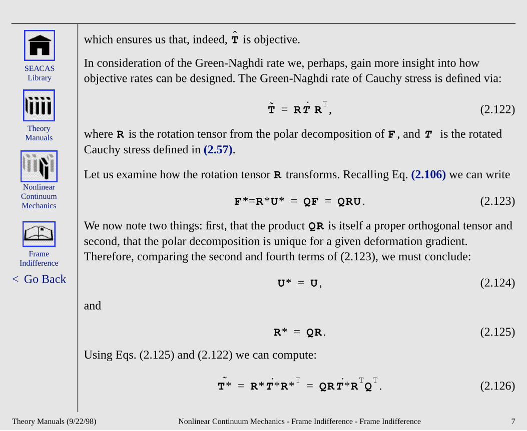
which ensures us that, indeed, is objective.

In consideration of the Green-Naghdi rate we, perhaps, gain more insight into how objective rates can be designed. The Green-Naghdi rate of Cauchy stress is define

, (2.122)

where is the rotation tensor from the polar decomposition of , and is the rotaCauchy stress defined in (2.57).

Let us examine how the rotation tensor transforms. Recalling Eq. (2.106) we can write

. (2.123)

We now note two things: first, that the product is itself a proper orthogonal tensosecond, that the polar decomposition is unique for a given deformation gradient. Therefore, comparing the second and fourth terms of (2.123), we must conclude:

, (2.124)

and

. (2.125)

Using Eqs. (2.125) and (2.122) we can compute:

. (2.126)

T

T RT ˙ RT

=

R F T

R

F*= R* U* QF QRU= =

QR

U* U=

R* QR=

T * R* T *˙ R*T

QRT *˙ RTQ

T= =


Theory Manuals (9

< Go Back

Frame Indifference


SEACAS Library

Theory Manuals

rence. It

.

can be on al elated ve stress dinate ann

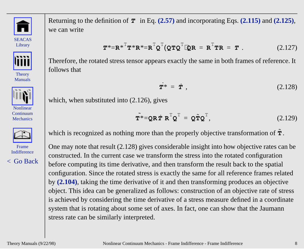
Returning to the definition of in Eq. (2.57) and incorporating Eqs. (2.115) and (2.125), we can write

. (2.127)

Therefore, the rotated stress tensor appears exactly the same in both frames of refefollows that

, (2.128)

which, when substituted into (2.126), gives

, (2.129)

which is recognized as nothing more than the properly objective transformation of

One may note that result (2.128) gives considerable insight into how objective rates constructed. In the current case we transform the stress into the rotated configuratibefore computing its time derivative, and then transform the result back to the spaticonfiguration. Since the rotated stress is exactly the same for all reference frames rby (2.104), taking the time derivative of it and then transforming produces an objectiobject. This idea can be generalized as follows: construction of an objective rate of is achieved by considering the time derivative of a stress measure defined in a coorsystem that is rotating about some set of axes. In fact, one can show that the Jaumstress rate can be similarly interpreted.

T

T *= R*TT* R*= R

TQ

TQTQ

T( )QR RTTR T = =

T *˙ T =

T * =QRT RTQ

TQTQ

T=

T


Theory Manuals (9

< Go Back

Frame Indifference


SEACAS Library

Theory Manuals

re
Finally, the Green-Naghdi rate can be manipulated further to a form resembling moclosely the form given for the Jaumann rate (Eq. (2.117)). We may write
, (2.130)

where we have used Eq. (2.42) to define , recalling also that this object is skew.

T Rtdd

RTTR( )RT

=

RRTT T TRR

T+ +=

T LTT TL+ +=

T TL L T–+=

L


Theory Manuals (9

< Go Back







SEACAS Library

Theory Manuals

Stress Measures

Balance Laws

Frame Indifference

Introduction RigidBodies


Two-Dimensional Formulations

Introduction

Plane Strain

Plane Stress

Axisymmetry

/22/98) Nonlinear Continuum Mechanics - Two-Dimensional Formulations 1

Theory Manuals (9

< Go Back

Two-Dimensional


SEACAS Library

Theory Manuals

work rain,

Introduction

In this section we very briefly discuss the adaptation of the three-dimensional frameto two-dimensional problems. We consider three cases of primary interest: plane stplane stress, and axisymmetry.

/22/98) Nonlinear Continuum Mechanics - Two-Dimensional Formulations - Introduction 2

Theory Manuals (9

< Go Back

Two-Dimensional


SEACAS Library

Theory Manuals

hold: r (for , no ted; 3)

be ero,

ion. onal wo

ents the in-

Plane Strain

The so-called plane strain assumption is appropriate when the following conditions 1) the object of interest can be geometrically described in a two-dimensional manneexample, by considering a cross section of a very long object); 2) once so idealizedloads on the structure act in the direction normal to the two-dimensional plane selecno significant displacement occurs normal to this plane; and 4) the variation of any quantity (stress, strain, displacement, etc.) in the direction normal to the plane can neglected. Conditions 3) and 4) require that all out-of-plane strain components be zgiving rise to the name plane strain.

The reader should refer to Figure 2.5 for the notational framework we will use. We

associate the third index, , (i.e., the z-coordinate) with the out-of-plane directAll of the continuum mechanical concepts we have developed for the three-dimensicase can then be straightforwardly applied to the current situation. We note that in tdimensions, one simply considers the large deformation boundary value problem summarized in Large Deformation Problems to be defined over a two-dimensional

domain with the unknown motion having two components rather than three.

Note that, in general, it is necessary, however, to keep track of some stress componassociated with the third dimension. This comes about due to the coupling betweenplane strains and the out-of-plane stresses. For example, considering infinitesimal elasticity for a moment, we have the following strain components equal to zero:

. (2.131)

i 3=

ϕ

E13 E23 E33 0= = =

/22/98) Nonlinear Continuum Mechanics - Two-Dimensional Formulations - Plane Strain 3

Theory Manuals (9

< Go Back

Two-Dimensional


SEACAS Library

Theory Manuals

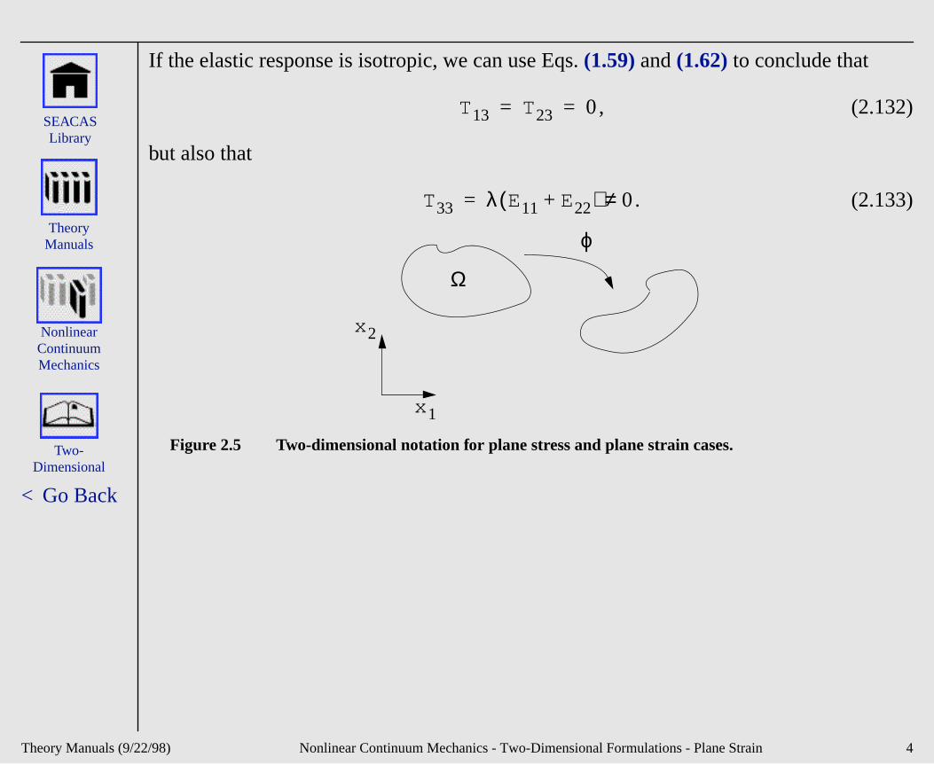
If the elastic response is isotropic, we can use Eqs. (1.59) and (1.62) to conclude that

, (2.132)

but also that

. (2.133)

Figure 2.5 Two-dimensional notation for plane stress and plane strain cases.

T13 T23 0= =

T33 λ E11 E22+( ) 0≠=

x 1

x 2

ϕ

Ω

/22/98) Nonlinear Continuum Mechanics - Two-Dimensional Formulations - Plane Strain 4

Theory Manuals (9

< Go Back

Two-Dimensional


SEACAS Library

Theory Manuals

hold: r; 2)

ction t in the is that

the value

again

Plane Stress

The plane stress assumption is appropriate when the following set of circumstances1) the object of interest can be geometrically described in a two-dimensional manneonce so idealized, no loads on the structure act in the direction normal to the two-dimensional plane selected; 3) no significant internal stress is generated in the direnormal to this plane; and 4) the variation of stress, strain, and in-plane displacemendirection normal to the plane can be neglected. Condition 3), in particular, makes thidealization most appropriate for thin, flat objects subject to in-plane loads. The factnonzero stresses are assumed to lie within the plane gives rise to the name plane stress.

The notation given in Figure 2.5 is appropriate for this class of problems, and as was case in plane strain, we simply specify the problem as a two-dimensional boundary

problem solving for the two-vector . Again, however, in describing the constitutive relations some knowledge of the third dimension must be maintained. Considering the linear elastic case for simplicity, we have

, (2.134)

from which we can conclude (for isotropy) that

, (2.135)

but also that

ϕ

T13 T23 T33 0= = =

E13 E23 0= =

/22/98) Nonlinear Continuum Mechanics - Two-Dimensional Formulations - Plane Stress 5

Theory Manuals (9

< Go Back

Two-Dimensional


SEACAS Library

Theory Manuals

ng is

, (2.136)

in general. Particularly when formulating plasticity problems, the out-of-plane strainiimportant to include as we shall see in later work.

E33

λ– E11 E22+( )λ 2µ+

----------------------------------- 0≠=

/22/98) Nonlinear Continuum Mechanics - Two-Dimensional Formulations - Plane Stress 6

Theory Manuals (9

< Go Back

Two-Dimensional


SEACAS Library

Theory Manuals

ry, and otation e

. The ear.

vector,

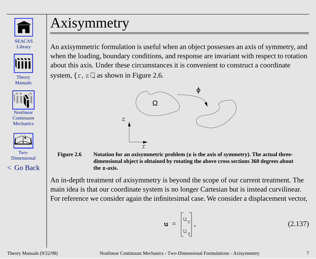
Axisymmetry

An axisymmetric formulation is useful when an object possesses an axis of symmetwhen the loading, boundary conditions, and response are invariant with respect to rabout this axis. Under these circumstances it is convenient to construct a coordinat

system, , as shown in Figure 2.6.

Figure 2.6 Notation for an axisymmetric problem (z is the axis of symmetry). The actual three-dimensional object is obtained by rotating the above cross sections 360 degrees about the z-axis.

An in-depth treatment of axisymmetry is beyond the scope of our current treatmentmain idea is that our coordinate system is no longer Cartesian but is instead curvilinFor reference we consider again the infinitesimal case. We consider a displacement

, (2.137)

r z,( )

r

z

ϕ

Ω

uur

uz

=

/22/98) Nonlinear Continuum Mechanics - Two-Dimensional Formulations - Axisymmetry 7

Theory Manuals (9

< Go Back

Two-Dimensional


SEACAS Library

Theory Manuals

e . One r

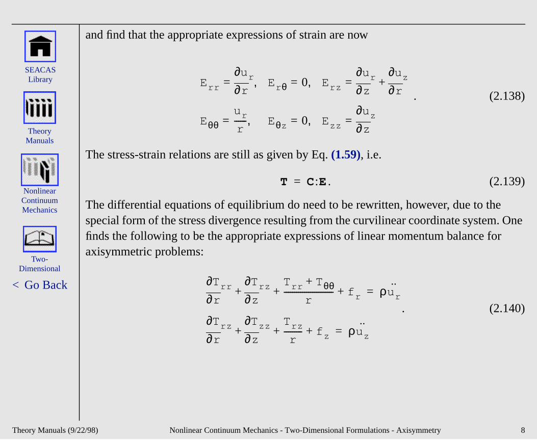
and find that the appropriate expressions of strain are now

. (2.138)

The stress-strain relations are still as given by Eq. (1.59), i.e.

. (2.139)

The differential equations of equilibrium do need to be rewritten, however, due to thspecial form of the stress divergence resulting from the curvilinear coordinate systemfinds the following to be the appropriate expressions of linear momentum balance foaxisymmetric problems:

. (2.140)

Err r∂∂ur ,= Er θ 0 ,= Erz z∂

∂ur

r∂∂uz+=

Eθθur

r------ ,= Eθz 0 ,= Ezz z∂

∂uz=

T C:E=

r∂∂Trr

z∂∂Trz Trr Tθθ+

r------------------------ f r+ + + ρur

˙=

r∂∂Trz

z∂∂Tzz Trz

r--------- f z+ + + ρuz

˙=

/22/98) Nonlinear Continuum Mechanics - Two-Dimensional Formulations - Axisymmetry 8

Theory Manuals (9

< Go Back







SEACAS Library

Theory Manuals

Stress Measures

Balance Laws

Frame Indifference


RigidBodies

Introduction


Introduction

The Degenerated Solid Approach

Plates and Shells

Beams

/22/98) Nonlinear Continuum Mechanics - Structural Components 1

Theory Manuals (9

< Go Back



SEACAS Library

Theory Manuals

solid ction ending a n we be

Introduction

Most discussion in this report has been primarily concerned with the description of deformation and stress in fully three-dimensional bodies. It is frequently desirable inmechanics to describe entities that are comparatively thin in at least one spatial direand perhaps in two. The former case is commonly referred to as a shell or plate (depon whether the entity is initially curved or flat), and the second case is referred to asbeam or truss (depending upon whether bending is to be considered). In this sectiobriefly discuss how the continuum mechanical framework we have constructed can adapted to these situations.

/22/98) Nonlinear Continuum Mechanics - Structural Components - Introduction 2

Theory Manuals (9

< Go Back



SEACAS Library

Theory Manuals

wn in ss ject.

hin ment

the

the

tion.

The Degenerated Solid Approach

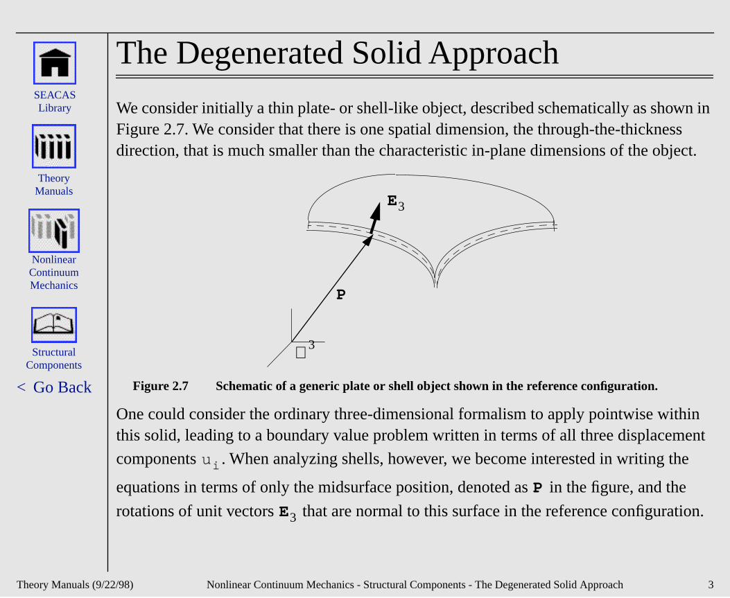
We consider initially a thin plate- or shell-like object, described schematically as shoFigure 2.7. We consider that there is one spatial dimension, the through-the-thicknedirection, that is much smaller than the characteristic in-plane dimensions of the ob

Figure 2.7 Schematic of a generic plate or shell object shown in the reference configuration.

One could consider the ordinary three-dimensional formalism to apply pointwise witthis solid, leading to a boundary value problem written in terms of all three displace

components . When analyzing shells, however, we become interested in writing

equations in terms of only the midsurface position, denoted as in the figure, and

rotations of unit vectors that are normal to this surface in the reference configura

ℜ 3

P

E3

ui

P

E3

/22/98) Nonlinear Continuum Mechanics - Structural Components - The Degenerated Solid Approach 3

Theory Manuals (9

< Go Back



SEACAS Library

Theory Manuals

face

ntity

ctural nts, h, one kness

g

tors

same

We can, therefore, express any reference point in the shell in terms of the midsur

position and the unit vector:

, (2.141)

where is a through-the-thickness coordinate ranging between and . The qua

is the local thickness of the shell referenced by .

As readers familiar with solid mechanics will be aware, the equations governing struobjects are conveniently written in terms of so-called stress resultants, or net mometorques, and forces, acting across cross sections. In the degenerated solid approactakes the fully three-dimensional equations of motion and performs through-the-thic

integration in terms of the appropriate coordinate (in this case ) to obtain governin

equations in terms of the midsurface displacements of points and rotations of vec

.

If the deformation is infinitesimal, so that reference and current coordinates are the

and changes in the thickness are insignificant, we obtain the shell equations of equilibrium by calculating

. (2.142)

X

P

X P ZE3+=

Zt2---–

t2---

t P

Z

P

E3

t

∇ T f+⋅ ρ–t

2

2

∂

∂ u+

Zd

t2---–

t2---

∫ 0=


Theory Manuals (9

< Go Back



SEACAS Library

Theory Manuals

ents,
The result will be a boundary value problem written in terms of midsurface displacemrotations, and stress resultants. We will return to this approach in more detail when discussing finite element procedures for treating the shell and plate equations in a companion report.

Theory Manuals (9

< Go Back



SEACAS Library

Theory Manuals

and t.

the

-

ssarily

sses in

with the

rally

e five

Plates and Shells

In addition to the concept of a degenerated solid, another important aspect of plateshell formulations is the specific kinematic description used to quantify displacemenReferring again to Figure 2.7, we describe the configuration mapping for any point in

shell in terms of the midsurface displacement and the normal vector rotation :

(2.143)

where we have actually made two kinematic assumptions: first, that the through-the

thickness deformation is negligible so that is the same coordinate as in (2.141); and

second, that normals to the midsurface (i.e., ) remain straight, although not nece

normal. This assumption leads to Mindlin plate theory where the rotation of vectors

with respect to the reference surface gives rise to transverse shear strains and strethe material.

Examining Eq. (2.143) we see that there are three dependent variables associated

mapping and three, in general, associated with the rotation . However, we gene

discard the component of producing rotation about . Thus, in general, there ar

dependent variables we seek to find in a plate or shell boundary value problem.

Φ q

ϕ X( ) Φ P( ) Zq E3×+=

Z

E3

E3

Φ q

q E3

/22/98) Nonlinear Continuum Mechanics - Structural Components - Plates and Shells 6

Theory Manuals (9

< Go Back



SEACAS Library

Theory Manuals

us,

librium

ne,

Beams

Beams can be considered within this framework also by considering two transversedimensions to be small when compared to the remaining one (i.e., beam length). Thrather than degenerating in one spatial dimension to obtain the resultant-based equiequations (as in (2.142)), we integrate in two. The result is usually a system with six dependent variables, described in terms of a one-dimensional object (a reference lirather than surface, in this case). Three of these correspond to the x , y , and z -components of the reference line displacement, and the other three correspond to rotations.

/22/98) Nonlinear Continuum Mechanics - Structural Components - Beams 7

Theory Manuals (9

< Go Back

RigidBodies






SEACAS Library

Theory Manuals

Stress Measures

Balance Laws

Frame Indifference


Introduction Structural Components

Rigid Bodies

Rigid Bodies

/22/98) Nonlinear Continuum Mechanics - Rigid Bodies 1

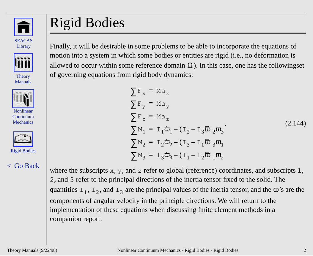
Theory Manuals (9

< Go Back

Rigid Bodies


SEACAS Library

Theory Manuals

of is

ingset

re the

Rigid Bodies

Finally, it will be desirable in some problems to be able to incorporate the equationsmotion into a system in which some bodies or entities are rigid (i.e., no deformation

allowed to occur within some reference domain ). In this case, one has the followof governing equations from rigid body dynamics:

, (2.144)

where the subscripts x , y , and z refer to global (reference) coordinates, and subscripts1, 2, and 3 refer to the principal directions of the inertia tensor fixed to the solid. The

quantities , , and are the principal values of the inertia tensor, and the ’s a

components of angular velocity in the principle directions. We will return to the implementation of these equations when discussing finite element methods in a companion report.

Ω

Fx∑ Max=

Fy∑ May=

Fz∑ Maz=

M1∑ I 1ω1 I 2 I 3–( )ω2ω3–=

M2∑ I 2ω2 I 3 I 1–( )ω3ω1–=

M3∑ I 3ω3 I 1 I 2–( )ω1ω2–=

I 1 I 2 I 3 ω

/22/98) Nonlinear Continuum Mechanics - Rigid Bodies - Rigid Bodies 2

SEACAS Library (8

< Go Back

tic

Adley, M.D., and Moxley, R.E., 1996 PENCURV/ABAQUS: A Simply Coupled Penetration Trajectory/Structural Dynamics Model for Deformable Projectiles Impacting Complex Curvilinear Targets, Technical Report SL-96-6, U.S. Army Engineer Waterways Experiment Station, Vicksburg, MS.

American National Standards Institute, 1978 American National Standards Programming Language FORTRAN ANSI X3.9-1978, American National Standards Institute, New York.

American Society for Testing and Materials, 19xx Annual Book of ASTM Standards: Section 3 - Metals Test Methods and Analytical Procedures, American Society for Testing and Materials, Philadelphia, Pennsylvania.

Attaway, S.W., 1990 Update of PRONTO 2D and PRONTO 3D Transient Solid Dynamics Program, SAND90-0102, Sandia National Laboratories, Albuquerque, NM.

Balmer, H.A. and Witmer, E.A., 1964 Theoretical-Experimental Correlation of Large Dynamic and Permanent Deformation of Impulsively Loaded Simple Structures, FDP-TDR-64-108, Air Force Flight Dynamics Laboratory, Wright-Patterson AFB, OH.

Bartels, R. and Daniel, J.W., 1973 “A conjugate gradient approach to nonlinear ellipboundary value problems in irregular regions,” in Lecture Notes in Mathematics, (A. Dold and B. Eckmann, eds.), Springer-Verlag, New York, pp. 1-11.

/26/98) Bibliography 1

SEACAS Library (8

< Go Back

M.

node

r

m

tes

Bathe, K.J. and Wilson, E.L., 1976 Numerical Methods in Finite Element Analysis, Prentice-Hall, Inc., New Jersey.

Beisinger, Z.E., 1984 SEACO: Sandia Engineering Analysis Department Code Output Data Base, SAND84-2004, Sandia National Laboratories, Albuquerque, N

Belytschko, T. and Bindelman, L.P., 1993 “Assumed strain stabilization of the eight hexahedral element,” Compter Methods in Applied Mechanics and Engineering, Vol. 105, pp. 225-260.

Belytschko, T. and Lin, J.I., 1985 “Eigenvalues and Stable Time Step for the BilineaMindlin Plate Element,” International Journal for Numerical Methods in Engineering, Vol. 21, pp. 1729-1745.

Belytschko, T. and Lin, J.I., 1987 “A Three-Dimensional Impact-Penetration Algorithwith Erosion,” Computers and Structures, Vol. 25, No. 1, pp. 95-104.

Belytschko, T., Lin, J.I. and Tsay, C.S., 1984 “Explicit Algorithms for the Nonlinear Dynamics of Shells,” Computer Methods in Applied Mechanics and Engineering, Vol. 42, pp. 225-251.

Belytschko, T. and Marchertas, A.H., 1974 “Nonlinear Finite Element Method for Plaand its Application to the Dynamic Response of Reactor Fuel Subassemblies,” Journal of Pressure Vessel Technology, ASME, pp. 251-157.


SEACAS Library (8

< Go Back

in

ost-

sical

p.

Belytschko, T. and Neal, M.O., 1991 “Contact-Impact by the Pinball Algorithm with Penalty and Lagrangian Methods,” International Journal Numerical Methods of Engineering, Vol. 31, pp. 547-572.

Belytschko, T., Ong, J.S.-J., Liu, W.K. and Kennedy, J.M., 1984 “Hourglass Control Linear and Nonlinear Problems,” Computer Methods in Applied Mechanics and Engineering, Vol. 43, pp. 251-276.

Belytschko, T., Schwer, L. and Klein, M.J., 1977 “Large Displacement Transient Analysis of Space Frames,” International Journal for Numerical Methods in Engineering, Vol. 11, pp. 65-84.

Benson, D.J. and Hallquist, J.O., 1990 “A Single Surface Contact Algorithm for the PBuckling Analysis of Structures,” Computer Methods in Applied Mechanics and Engineering, Vol. 78, pp. 141-163.

Benz, W., 1988 “Applications of Smooth Particle Hydrodynamics (SPH) to AstrophyProblems,” Computational Physics Commuinications, Vol. 48, pp. 97-105.

Benz, W., 1990 “Smooth Particle Hydrodynamics: A Review,” in The Numerical Modeling of Stellar Pulsation, (J.R. Buchler, ed.), Kluwer, Dordrecht, Netherlands,269.

Bergmann, V.L., 1991 Transient Dynamic Analysis of Plates and Shells with PRONTO 3D, SAND91-1182, Sandia National Laboratories, Albuquerque, NM.


SEACAS Library (8

< Go Back

”,

Bertsekas, D.P., 1982 Constrained Optimization and Lagrange Multiplier Methods, Academic Press, New York.

Biffle, J.H., 1981 JAC--A Two-Dimensional Finite Element Computer Program for the Nonlinear Response of Solids with the Conjugate Gradient Method, SAND81-0998, Sandia National Laboratories, Albuquerque, NM.

Biffle, J.H., 1984 JAC - A Two-Dimensional Finite Element Computer Program for the Nonlinear Quasi-Static Response of Solids with the Conjugate Gradient Method, SAND81-0998, Sandia National Laboratories, Albuquerque, NM.

Biffle, J.H., 1993 JAC3D - A Three-Dimensional Finite Element Computer Program for the Nonlinear Quasi-Static Response of Solids with the Conjugate Gradient Method, SAND87-1305, Sandia National Laboratories, Albuquerque, NM.

Biffle, J.H. and Gubbels, M.H., 1976 WULFF - A Set of Computer Programs for the Large Displacement Dynamic Response of Three Dimensional Solids, SAND76-0096, Sandia National Laboratories, Albuquerque, NM.

Biffle, J.H. and Stone, C.M., 1989 “Personal communications,” Applied Mechanics Division, Sandia National Laboratories, Albuquerque, NM.

Bishop, R.F., Hill, R., and Mott, N.F., 1945 “The theory of indentation and hardnessProceedings of the Royal Society, Vol. 57 (3), pp. 147-159.


SEACAS Library (8

< Go Back l

sient

Blacker, T.D., 1988 FASTQ Users Manual Version 1.2, SAND88-1326, Sandia NationaLaboratories, Albuquerque, NM.

Boaz, M.L., 1966 Mathematical Methods in the Physical Sciences, John Wiley and Sons, New York, NY.

Budiansky, B. and O’Connell, R.J., 1976 “Elastic moduli of a cracked solid,” Computer Methods in Applied Mechanics and Engineering, Vol. 12, pp. 81-97.

CRAY Research, Inc., 1989 Volume 3: UNICOS Math and Scientific Library Reference Manual, SR-2081 5.0.

Campbell, P.M., 1988 Some New Algorithms for Boundary Values Problems in Smooth Particle Hydrodynamics, DNA-TR-88-286.

Carpenter, N.J., Taylor, R.L. and Katona, M.G., 1991 “Lagrange Constraints for TranFinite Element Surface Contact,” International Journal for Numerical Methods in Engineering, Vol. 32, 103-128.

Chait, R., 1972 “Factors influencing the strength differential of high strength steels”,Metalurgical Transactions A, Vol. 3, pp. 365-371.

Chakarabarty, J., 1987 Theory of Plasticity, McGraw-Hill Book Company, New York, pp. 306-315, 342-350.


SEACAS Library (8

< Go Back

n,

Chaudhary, A.B. and Bathe, K.J., 1986 “A Solution Method for Static and Dynamic Analysis of Three-Dimensional Contact Problems with Friction,” Computers and Structures, Vol. 24, No. 6, pp. 855-873.

Cheung, C.Y. and Cebon, D., 1997 “Experimental Study of Pure Bitumens in TensioCompression, and Shear,” Journal of Rheology, Vol. 41, No. 1, pp. 45-73.

Chou, T.S., 1989 The Dynamic Response at High-Explosive Inert-Solid Interface as Predicted by Finite Difference/Element Computer Programs, Tech. Rep. MLM-3562, EG&G Mound Applied Technologies, Miamisburg, OH.

Cloutman, L.D., 1990(a) Basics of Smoothed Particle Hydrodynamics, Lawrence Livermore National Laboratory, Livermore, CA, report UCRL-ID-103698.

Cloutman, L.D., 1990(b) “An Evaluation of Smoothed Particle Hydrodynamics,” Proceedings of The NEXT Free-Lagrange Conference, Jackson Lake Lodge, Moran, WY, June 3-7.

Cohen, M. and Jennings, P.C., 1983 “Silent Boundary Methods,” in Computational Methods for Transient Analysis, (Belytschko, T. and Hughes, T.J.R., eds.), North-Holland.

Cole, R.H., 1965 UnderWater Explosions, Dover Publications.


SEACAS Library (8

< Go Back

rk,

in

s

r

”

Concus, P., Golub, G.H. and O’Leary, D.P., 1976 “A generalized conjugate gradientmethod for the numerical solution of elliptic partial differential equations,” in Sparse Matrix Computations , (J.R. Bunch and D.J. Rose, eds.), Academic Press, New Yopp. 309-332.

Courant, R., Friedrichs, K.O. and Lewy, H., 1928 Mathematical Annotations, Vol. 100, p. 32.

Crismann, J.M. and Zapas, L.J., 1979 “Creep Failure and Fracture of Polyethylene Uniaxial Extension,” Polymer Engineering Science, Vol. 19, pp. 99-103.

Curnier, A. and Alart, P., 1988 “A Generalized Newton Method for Contact Problemwith Friction,” Journal de Mecanique Theorique et Appliquee, Vol. 7, 67-82.

Daniel, J.W., 1967 “The conjugate gradient method for linear and nonlinear operatoequations,” SIAM Journal of Numerical Analysis, Vol. 4, no. 1, pp. 10-26.

Dennis, J.E. and Schnabel, R.B., 1996 Numerical Methods for Unconstrained Optimization and Nonlinear Equations, Society for Industrial and Applied Mathematics, Philadelphia.

Dienes, J.K., 1979 “On the analysis of rotation and stress rate in deforming bodies,Acta Mechanica, Vol. 32, pp. 217-232.


SEACAS Library (8

< Go Back

e

Dobratz, B.M., 1981 LLNL Explosives Handbook, Properties of Chemical Explosives and Explosive Simulants, UCRL-52997, Lawrence Livermore National Laboratory,Livermore, CA.

Duffey, T.A., and Macek, R.W., 1997 “Non-normal impact of earth penetrators”, Proceedings of the International Symposium on Penetration and Impact Problems (ICES'97), San Jose, Costa Rica.

Engleman, R. and Jaeger, Z., 1987 Theoretical Aids for Improvement of Blasting Efficiencies in Oil Shale and Rocks, Tech. Rep AP-TR-12/87, Soreq Nuclear Research Center, Yavne, Israel.

Ferry, 1950 ???

Flanagan, D.P. and Belytschko, T., 1981 “A Uniform Strain Hexahedron and Quadrilateral with Orthogonal Hourglass Control,” International Journal for Numerical Methods in Engineering, Vol. 17, pp. 679-607.

Flanagan, D.P. and Belytschko, T., 1984 “Eigenvalues and Stable Time Steps for thUniform Hexahedron and Quadrilateral,” Journal of Applied Mechanics, Vol. 51, pp. 35-40.

Flanagan, D.P., Mills-Curran, W.C., and Taylor, L.M., 1986 SUPES - A Software Utilities Package for the Engineering Sciences, SAND86-0911, Sandia National Laboratories, Albuquerque, NM.


SEACAS Library (8

< Go Back

in

,”

ets

m

Flanagan, D.P. and Taylor, L.M., 1987 “An accurate numerical algorithm for stress integration with finite rotations,” Computer Methods in Applied Mechanics and Engineering, Vol. 62, pp. 305-320.

Flanagan, D.P. and Taylor, L.M., 1987 “On the Analysis of Rotation and Stress RateDeforming Bodies,” Computer Methods in Applied Mechanics and Engineering, Vol. 62, pp. 305-320.

Fletcher, R. and Reeves, C.M., 1964 “Function minimization by conjugate gradientsThe Computer Journal, Vol. 7, pp. 149-154.

Forrestal, M.J., Altman, B.S., Cargile, J.D., and Hanchak, S.J., 1994 “An empirical equation for penetration depth of ogive-nose projectiles into concrete targets”, International Journal of Impact Engineering, Vol. 15, pp. 395-405.

Forrestal, M.J., Brar, N.S., and Luk, V.K., 1991 “Penetration of strain-hardening targwith rigid spherical-nose rods”, ASME Journal of Applied Mechanics, Vol. 58, pp. 7-10.

Forrestal, M.J. and Luk, V.K., 1991 “Penetration into soil targets”, International Journal of Impact Engineering, Vol. 12, pp. 427-444.

Forrestal, M.J., Okajima, K., and Luk, V.K., 1988 “Penetration of 6061-T651 aluminutargets with rigid long rods”, ASME Journal of Applied Mechanics, Vol. 55, pp. 755-760.


SEACAS Library (8

< Go Back el

ncrete

ntact

Forrestal, M.J., and Tzou, D.Y., 1996 “A spherical cavity-expansion penetration modfor concrete targets”, International Journal of Solids Structures (accepted).

Forrestal, M.J., Tzou, D.Y., Askari, E., and Longcope, D.B., 1995 “Penetration into ductile metal targets with rigid spherical-nose rods”, International Journal of Impact Engineering, Vol. 16, pp. 699-710.

Freudenthal, 1963 ???

Frew, D.J., Hanchak, S.J., Green, M.L., and Forrestal, M.J., 1997 “Penetration of cotargets with ogive-nose steel rods”, International Journal of Impact Engineering, (submitted).

Frost and Ashby, 19?? Deformation Mechanisms Maps, ???.

Fung, Y.C., 1965 Foundations of Solid Mechanics, Prentice-Hall, Englewood Cliffs, New Jersey.

Fung, Y.C., 1977 A First Course in Continuum Mechanics, 2nd edition, Prentice-Hall, Englewood Cliffs, New Jersey.

Gallego, F.J. and Anza, J.J., 1989 “A Mixed Finite Element Model for the Elastic CoProblem,” International Journal for Numerical Methods in Engineering, Vol. 28, 1249-1264.


SEACAS Library (8

< Go Back tion

,

ts of

Giannakopoulos, A.E., 1989 “The Return Mapping Method for the Integration of FricConstitutive Relations,” Computers and Structures, Vol. 32, 157-167.

Gilkey, A.P., 1988 ALGEBRA - A Program that Algebraically Manipulates the Output of a Finite Element Analysis (EXODUS Version), SAND88-1431, Sandia National Laboratories, Albuquerque, NM.

Gilkey, A.P. and Glick, J.H., 1989 BLOT - A Mesh and Curve Plot Program for the Output of a Finite Element Analysis, SAND88-1432, Sandia National LaboratoriesAlbuquerque, NM.

Gilkey, A.P. and Sjaardema, G.D., 1989 GEN3D: A GENESIS Database 2D to 3D Transformation Program, SAND89-0485, Sandia National Laboratories, Albuquerque, NM.

Gingold, R.A. and Monaghan, J.J., 1982 “Kernel Estimates as a Basis for General Particle Methods in Hydrodynamics,” Journal Computational Physics, Vol. 46, pp. 429-453.

Glowinski, R. and LeTallec, P., 1989 Augmented Lagrangian and Operator Splitting Methods in Nonlinear Mechanics, SIAM, Philadelphia.

Goodier, J.N. 1965 “On the mechanics of indentation and cratering in the solid targestrain-hardening metal by impact of hard and soft spheres”, Proceedings of the 7th Symposium on Hypervelocity Impact III, pp. 215-259.


SEACAS Library (8

< Go Back

M.

Grady, D., 1983 “The Mechanics of Fracture Under High-rate Stress Loading,” in William Prager Syposium on Mechanics of Geomaterials: Rocks, Concretes and Soils, (Bazant, Z.P., ed.).

Guenther, C., Hicks, D.L. and Swegle, J.W., 1994 Conservative Smoothing versus Artificial Viscosity , SAND94-1853, Sandia National Laboratories, Albuquerque, N

Gurtin, M.E., 1981 An Introduction to Continuum Mechanics, Academic Press, Inc.

Hallquist, J.O., 1981 User’s Manual for DYNA3D and DYNAP, Lawrence Livermore National Laboratory, Livermore, CA.

Hallquist, J.O., 1982 User’s Manual for DYNA2D - An Explicit Two-Dimensional Hydrodynamic Finite Element Code with Interactive Rezoning, Lawrence Livermore National Laboratory, Livermore, CA.

Hallquist, J.O., 1984 NIKE3D: An Implicit, Finite Deformation, Finite Element Code for Analyzing the Static and Dynamic Response of Three Dimensional Solids, UCID-18822, Lawrence Livermore National Laboratory, Livermore, CA.

Hallquist, J.O., 1984 User’s Manual for DYNA2D: An Explicit Two-Dimensional Hydrodynamic Finite Element Code with Interactive Rezoning, Rev. 2, UCID-18756, Lawrence Livermore National Laboratory, Livermore, CA.


SEACAS Library (8

< Go Back

tact-

al

,

Hallquist, J.O., 1986 NIKE2D: A Vectorized Implicit, Finite Deformation Finite Element Code for Analyzing the Static and Dynamic Response of 2-D Solids withInteractive Rezoning and Graphics, UCID-19677, Lawrence Livermore National Laboratory, Livermore, CA.

Hallquist, J.O., Goudreau, G.L. and Benson, D.J., 1985 “Sliding Interfaces with ConImpact in Large-Scale Lagrangian Computations,” Computer Methods in Applied Mechanics and Engineering, Vol. 51, 107-137.

Hallquist, J.O. and Benson, D.J., 1986 “A comparison of an Implicit and Explicit Implementation of the Hughes-Liu Shell,” in Finite Element Methods for Plate and Shell Structures, Volume 1: Element Technology, (Hughes, T.J.R. and Hinton, E., eds.), Pineridge Press International, Swansea, U.K., pp. 394-430.

Hallquist, J.O. and Benson, D.J., 1987 User’s Manual for DYNA3D: Nonlinear Dynamic Analysis of Structures, Rev. 3, UCID-19592, Lawrence Livermore NationLaboratory, Livermore, CA.

Harding, D.C., Attaway, S.W., Neilsen, J., Blacker, T.D. and Pierce, J., 1992 Evaluation of Four Multiple Package Crush Environment to the Common Package, Model 1, Plutonium Air Transport Container , SAND92-0278, Sandia National LaboratoriesAlbuquerque, NM.

Harlow, F.H., 1988 “PIC and its Progeny,” Computational Physics Communications, Vol. 48, pp. 1-10.


SEACAS Library (8

< Go Back

ear

,

l ’s

Hearmon, R. F. S., 1961 An Introduction to Applied Anisotropic Elasticity , Oxford University Press, Oxford, England.

Herrman and Peterson, 1968 ???

Heinstein, M.W., Attaway, S.W., Mellow, F.J. and Swegle, J.W., 1993 A General-Purpose Contact Detection Algorithm for Nonlinear Structural Analysis Codes, SAND92-2141, Sandia National Laboratories, Albuquerque, NM.

Hestenes, M.R. and Stiefel, E., 1952 “Methods of conjugate gradients for solving linsystems,” Journal of Research of the National Bureau of Standards, Vol. 49, pp. 409-436.

Hibbitt, Karlsson and Sorensen, Inc., 1989 ABAQUS Users Manual, Version 4-8, Hibbitt, Karlsson and Sorensen, Inc., Providence, Rhode Island.

Hibbitt, Karlsson and Sorensen, Inc., 1992 Contact Calculations with ABAQUS - ABAQUS Explicit Users Manual, Hibbitt, Karlsson and Sorensen, Inc., ProvidenceRhode Island.

Hicks, D.L., 1978 “Stability Analysis of WONDY (A Hydrocode Based on the ArtificiaViscosity Method of von Neumann and Richtmyer) for a Special Case of MaxwellLaw,” Mathematics of Computation, Vol. 32, pp. 1123-1130.


SEACAS Library (8

< Go Back ion

um

,

Hilber, Hughes, and Taylor, 1977 “Improved Numerical Dissipation for Time IntegratAlgorithms in Structural Dynamics,” Earthquake Engineering and Structural Dynamics, Vol. 5, pp.283-292.

Hill, R., 1948 A Theory of Earth Movement Near a Deep Underground Explosion, Memo No. 21-48, Armament Research Establishment, Fort Halstead, Kent, UK.

Hill, R., 1950 The Mathematical Theory of Plasticity, Oxford University Press, London.

Holcomb, D.J., 1985 “Results of the 55 Day Consolidation Test,” Internal Memorandto J. Stormont, 6332, Sandia National Labs, Albuquerque, NM.

Holcomb, D.L and Hannum, D.W., 1982 Consolidation of Crushed Salt Backfill Under Conditions Applicable to the WIPP Facility, SAND82-0630, Sandia National Labs,Albuquerque, NM.

Holcomb, D.J. and Shields, M.F., 1987 Hydrostatic Consolidation of Crushed Salt with Added Water, SAND87-1990, Sandia National Labs, Albuquerque, NM.

Holden, J.T., 1972 “On the finite deflections of thin beams,” International Journal of Solids and Structures, Vol. 8, pp. 1051-1055.

Hopkins, H.G., 1960 “Dynamic expansion of spherical cavities in metals”, Progress in Solid Mechanics, Vol. 1, (Editors I. Sneddon and R. Hill), North Holland, New Yorkpp. 85-164.


SEACAS Library (8

< Go Back stic

of

f

Huang, J., 1969 “Transient Interaction of Plane Acoustic Waves with a Spherical ElaShell,” Journal Acoustical Society of America, Vol. 45, pp. 661-670.

Hughes, T.J.R., 1987 The Finite Element Method: Linear Static and Dynamic Finite Element Analysis, Prentice-Hall, Inc., Englewood Cliffs, New Jersey.

Hughes, T.J.R. and Winget, J., 1980 “Finite rotation effects in numerical integration rate constitutive equations arising in large-deformation analysis,” International Journal for Numerical Methods in Engineering, Vol. 15, No. 12, pp. 1862-1867.

Ide,Y. and White, J.L., 1977 “Investigation of Failure During Elongational Flow of Polymer Melts,” Journal of Non-Newtion Fluid Mechanics, Vol. 2, pp. 281-298.

Ide,Y. and White, J.L., 1979 “Experimental Study of Elongational Flow and Failure oPolymer Melts,” Journal of Applied Polymer Science,Vol. 22, pp. 1061-1079.

International Nickel Company, Inc., The, 1964 18% Nickel Maraging Steels, New York, NY.

Irons, B. and Elsawaf, A., 1977 “The conjugate Newton algorithm for solving finite element equations,” Formulations and Computation Algorithms in Finite Element Analysis, (K.J. Bathe and W. Wunderlich, eds.), MIT Press, pp. 655-672.

Johnson, G.C. and Bammann, D.J., 1984 “A discussion of stress rates in finite deformation bodies,” International Journal of Solids and Structures, Vol. 20, no. 8, pp. 725-737.


SEACAS Library (8

< Go Back ate in

puter

Johnson, G.C. and Bammann, D.J., 1984 “On the Analysis of Rotation and Stress RDeforming Bodies,” International Journal of Solids and Structures, Vol. 20, No. 8, pp. 725-737.

Johnson, G.R., 1983 Development of Strength and Fracture Models for Computations Involving Severe Dynamic Loading, Vol. I: Strength and Fracture Models, Tech. Rep. AFATL-TR-83-05, Air Force Armament Laboratory.

Johnson, G.R., 1988 “Implementation of simplified constitutive models in large comcodes,” in Dynamic Constitutive/Failure Models, (A. M. Rajendran and T. Nichols, eds.), pp. 409-426, Dayton, OH.

Johnson, G.R. and Holmquist, T.J., 1989 Test Data and Computational Strength and Fracture Model Constants for 23 Materials Subjected to Large Strains, High Strain Rates, and High Temperatures, Tech. Rep. LA-11463-MS, Los Alamos National Laboratory, Los Alamos, NM.

Johnson, G.R., Stryk, R.A., Holmquist, T.J., and Beissel, S.R., 1996 User Instructions for the 1996 version of the EPIC Code, Alliant Techsystems Inc., Hopkins, MN.

Johnson, G.R., Stryk, R.A., Holmquist, T.J., and Beissel, S.R., 1997 EPIC 97 (software to be released), Alliant Techsystems Inc., Hopkins, MN.

Johnson, J.B., 1989 “Personal communication,” USACRREL, Building 4070, Ft. Wainwrite, Alaska.


SEACAS Library (8

< Go Back

of

Ju, J.-W. and Taylor, R.L., 1988 “A Perturbed Lagrangian Formulation for the FiniteElement Solution of Nonlinear Frictional Contact Problems,” Journal of Theoretical and Applied Mechanics, Vol. 7, 1-14.

Kamei, E. and Onogi, 1975 “Extensional and Fractural Properties of Monodisperse Polystyrenes at Elevated Temperatures,” Applied Polymer Symposium, Vol 27, pp. 19-46.

Kaplan, W., 1959 Advanced Calculus, Addison-Wesley Publishing, Reading MA.

Kelley, C.T., 1995 Iterative Methods for Linear and Nonlinear Equations, Society for Industrial and Applied Mathematics, Philadelphia.

Kerighan, B.W., and Ritchie, D.M., 1978 The C Programming Language, Prentice-Hall, Inc., New Jersey.

Key, S.W., Beisinger, Z.E. and Kreig, R.D., 1978 HONDO II -A Finite Element Computer Program for the Large Deformation Dynamics Response of Axisymmetric Solids, SAND78-0422, Sandia National Laboratories, Albuquerque,NM.

Kikuchi, N. and Song, Y.J., 1981 “Penalty/Finite Element Approximations of a ClassUnilateral Problems in Linear Elasticity,” Quarterly of Applied Mathematics, Vol. 39, 1-22.


SEACAS Library (8

< Go Back

tion,”

eory

Kikuchi, N. and Oden, J.T., 1988 Contact Problems in Elasticity: A Study of Variational Inequalities and Finite Element Methods, SIAM, Philadelphia.

Kipp, M.E. and Grady, D.E., 1978 Numerical Studies of Rock Fragmentations, SAND79-1582, Sandia National Laboratories, Albuquerque, NM.

Kipp, M.E., Grady, D.E. and Chen, E.P., 1980 “Strain-rate Dependent Fracture InitiaInternational Journal of Fracture , Vol. 16, pp. 471-478.

Kipp, M.E. and Lawrence, R.J., 1982 WONDY V - A One-Dimensional Finite-Difference Wave Propagation Code, SAND81-0930, Sandia National Laboratories,Albuquerque, NM.

Krieg, R.D., 1978 A Simple Constitutive Description for Soils and Crushable Foams, SC-DR-72-0883, Sandia National Laboratories, Albuquerque, NM.

Krieg, R.D. and Key, S.W., 1976 “Implementation of a Time Dependent Plasticity Thinto Structural Computer Programs,” Constitutive Equations in Viscoplasticity: Computational and Engineering Aspects, Vol. 20, ASME, New York, p. 125.

Kreig, R.D. and Krieg, D.B., 1977 “Accuracies of numerical solution methods for theelastic-perfectly plastic model,” ASME Journal of Pressure Vessel Technology, Vol. 99, pp. 510-515.


SEACAS Library (8

< Go Back

es

n for ,”

nal

Kuszmaul, J.S., 1987 “A New Constitutive Model for Fragmentation of Rock Under Dynamic Loading,” in Proceedings of the Second International Symposium on Fragmentation by Blasting, pp. 412-423, Keystone, CO.

Kuszmaul, J.S., 1987 “A Technique for Predicting Fragmentation and Fragment SizResulting from Rock Blasting,” in Proceedings of the 28th U.S., Symposium on Rock Mechanics, Tucson, AZ.

Lai, W.M, Rubin, D. and Krempl, E., 1993 Introduction to Continuum Mechanics, 3rd edition, Pergamon Press.

Laursen, T.A., 1994 “The Convected Description in Large Deformation Frictional Contact Problems,” International Journal of Solids and Structures, Vol. 31, pp. 669-681.

Laursen, T.A. and Simo, J.C., 1993 “A Continuum-Based Finite Element Formulatiothe Implicit Solution of Multibody, Large Deformation Frictional Contact ProblemsInternational Journal for Numerical Methods in Engineering, Vol. 36, 3451-3485.

Laursen, T.A. and Simo, J.C., 1993 “Algorithmic Symmetrization of Coulomb FrictioProblems Using Augmented Lagrangians,” Computer Methods in Applied Mechanics and Engineering, Vol. 108, 133-146.

Leaderman, 1943 ???


SEACAS Library (8

< Go Back.

ds

th of

e,

Lee, E., Finger, M. and Collins, W., 1973 JWL Equation of State Coefficients for High Explosives, UCID-16189, Lawrence Livermore National Laboratory, Livermore, CA

Lee, Radok, and Woodward, 1959 ???

Lenard, M.L., 1976 “Convergence conditions for restarted conjugate gradient methowith inaccurate line searches,” Mathematical Programming, Vol. 10, pp. 32-51.

Libersky, L. and Petschek, A.G., 1990 “Smooth Particle Hydrodynamics with StrengMaterials,” Proceedings of The NEXT Free-Lagrange Conference, Jackson Lake Lodge, Moran, WY, June 3-7.

Longcope, D.B., 1991 Coupled Bending/Lateral Load Modeling of Earth Penetrators, SAND90-0789, Sandia National Laboratories, Albuquerque, NM.

Longcope, D.B., 1996 Oblique Penetration Modeling and Correlation with Field Tests into a Soil Target, SAND96-2239, Sandia National Laboratories, AlbuquerquNM.

Longcope, D.B. and Tabbara, M.R., 1998 Modeling of Oblique Earth Penetration Using Cavity Expansion Loading with Surface Effects, SAND98-xxxx, Sandia National Laboratories, Albuquerque, NM, in preparation.

Lovejoy, S.C. and Whirley, R.G., 1990 DYNA3D Example Problem Manual, UCRL-MA-105259, Lawrence Livermore National Laboratory, Livermore, CA.


SEACAS Library (8

< Go Back

ids

ons,”

Luenberger, D.G., 1984 Linear and Nonlinear Programming, 2nd ed., Addison-Wesley, Reading, MA.

Lucy, L.B., 1977 “A Numerical Approach to the Testing of the Fission Hypothesis,” Astrophysics Journal, Vol. 82, pp. 1013-1024.

Luk, V.K. and Piekutowski, A.J., 1991 “An analytical model on penetration of erodinglong rods into metallic targets,” International Journal of Impact Engineering, Vol. 11, pp. 323-340.

Lysmer, J. and Kuhlemeyer, R.L., 1979 “Finite Dynamic Model for Infinite Media,” Journal of the Engineering Mechanics Division of ASCE, pp. 859-877.

Malkin, A. Y. and Petrie, C.J.S., 1997 “Some Conditions for Rupture of Polymer Liquin Extension,” Journal of Rheology, Vol. 41 (1), pp. 1-25.

Malvern, L.E., 1969 Introduction to the Mechanics of a Continuous Medium, Prentice-Hall, Inc., New Jersey, pp. 226-228.

Marsden, J.E. and Hughes, T.J.R., 1983 Mathematical Foundations of Elasticity, Prentice-Hall, Englewood Cliffs, New Jersey.

Matthies, H. and Strang, G., 1979 “The Solution of Nonlinear Finite Element EquatiInternational Journal for Numerical Methods in Engineering, Vol. 14, 1613-1626.

McClelland, 19?? ???


SEACAS Library (8

< Go Back

in

McClure, C., 1993 Preliminary Report on Explosive Field Tests in Support of the Hull Deformation/Rupture Study, NSWC Report NSWCDD/TN-93/94.

Mendelson, A., 1968 Plasticity: Theory and Application, The Macmillan Company, New York, pp. 138-156.

Metzinger, K., Attaway, S. and Mello, F., 1991 “Bobbin Stresses Generated by WireWinding,” First International Conference of Web Handling, Oklahoma State University, Stillwater, OK.

Michalowski, R. and Mroz, Z., 1978 “Associated and Non-Associated Sliding Rules Contact Friction Problems,” Archives of Mechanics, Vol. 30, 259-276.

Mills-Curran, W.C., 1988 EXODUS: A Finite Element File Format for Pre- and Post-Processing, SAND87-2997, Sandia National Laboratories, Albuquerque, NM.

Mindlin, R.D., 1951 “Influence of Rotatory Inertia and Shear on Flexural Motions of Isotropic, Elastic Plates,” Journal of Applied Mechanics, Vol. 18, pp. 31-38.

Monaghan, J.J., 1982 “Why Particle Methods Work,” SIAM Journal Scientific Statistical Computing, Vol. 3, pp. 422-433.

Monaghan, J.J., 1985 “Particle Methods for Hydrodynamics,” Computational Physics Reports, Vol. 3, pp. 71-124.


SEACAS Library (8

< Go Back

ent

of

Monaghan, J.J., 1988 “An Introduction to SPH,” Computational Physics Communications, Vol. 48, pp. 89-96.

Monaghan, J.J. and Gingold, R.A., 1983 “Shock Simulation by the Particle Method SPH,” Journal of Computational Physics, Vol. 52, pp. 374-389.

Morland and Lee, 1960 ???

Mungiza, A., Owen, D.R.J. and Bicanic, N., 1995 “A Combined Finite-Discrete ElemMethod in Transient Dynamics of Fracturing Solids,” Engineering Computations, Vol. 12, pp. 145-174.

Muki and Sternberg, 1961 ???

Neilsen, M.K., Morgan, H.S. and Krieg, R.D., 1986 A Phenomenological Constitutive Model for Low Density Polyurethane Foams, SAND86-2927, Sandia National Laboratories, Albuquerque, NM.

Nemat-Nasser, S., Chung, D. and Taylor, L.M., 1989 “Phenomenological modeling rate-dependent plasticity for high strain rate problems,” Mechanics of Materials, Vol. 7, No. 4, pp. 319-344.

Newmark, N.M., 1959 “A Method of Computation for Structural Dynamics,” Journal of the Engineering Mechanics Division, ASCE, 67-94.


SEACAS Library (8

< Go Back

-

ablish

s on

Ogden, R.W., 1987 “Recent advances in the phenomenological theory of rubber elasticity,” Rubber Chemistry and Technology, Vol. 59, pp. 361-383.

Parisch, H., 1989 “A Consistent Tangent Stiffness Matrix for Three Dimensional NonLinear Contact Analysis,” International Journal for Numerical Methods in Engineering, Vol. 28, 1803-1812.

Patel, N.R. and Finnie, I., 1969 ???, Report UCRL-13420, Lawrence Livermore Laboratory, Livermore, CA.

Pearson, G.H. and Connelly, R.W., 1982 “The Use of Extensional Rheometry to EstOperating Parameters for Stretching Processes,” Journal of Applied Polymer Science, Vol. 27, pp. 969-981.

Perzyna, P., 1966 “Fundamental Problems in Viscoplasticity,” in Recent Advances in Applied Mechanics, Academic Press, New York, pp. 243-377.

Pfeiffle, T.W. and Senseny, P.E., 1985 Permeability and Consolidation of Crushed Salt from the WIPP Site, Topical Report RSI-0278, RE/SPEC Inc., Rapid City, SD.

Pilkey, W.D. and Wunderlich, W., 1994 Mechanics of Structures: Variational and Computational Methods, CRC Press.

Plimpton, S.J., 1990 “Molecular Dynamics Simulations of Short-Range Force System1024-Node Hypercubes,” Proceedings of the Fifth Distributed Memory Computing Conference, Charleston, SC.


SEACAS Library (8

< Go Back

et

s

Powell, M.J.D., 1977 “Restart procedures for the conjugate gradient method,” Mathematical Programming, Vol. 12, pp. 242-254.

Ralston, A. and Wilf, H.S., 1960 Mathematical Methods of Digital Computers, John Wiley and Sons Inc., New York, pp. 62-72.

Ratigan and Wagner, 19?? ???

Rebelo, N., Nagtegaal, J.C. and Hibbitt, H.D., 1990 “Finite Element Analysis of SheForming Processes,” International Journal for Numerical Methods in Engineering, Vol. 30, 1739-1758.

Reedy, J.E.D., 1990 “Memo: Code corrections to pronto’s soils and crushable foammodel,” Applied Mechanics Division, Sandia National Laboratories, Albuquerque,NM.

Richtmyer, R.D. and Morton, K.W., 1967 Difference Methods for Initial Value Problems, Interscience, New York.

Rivlin, R.S., 1948 “???”, Philosophical Transactions of the Royal Society of London, A, pp. 459-490.

Schoof, L.A. and Yarberry, V.R., 1994 EXODUS II: A Finite Element Data Model, SAND92-2137, Sandia National Laboratories, Albuquerque, NM.


SEACAS Library (8

< Go Back r

e of s and

ins:

ent

Schreyer, H.L., Kulak, R.F. and Kramer, J.M., 1979 “Accurate numerical solutions foelastic-plastic models,” ASME Journal of Pressure Vessel Technology, Vol. 101, pp. 226-234.

Schwarzl and Staverman, 1952 ???

Silling, S. A., 1991 CTH Reference Manual: Viscoplastic Models, SAND91-0292, Sandia National Laboratories, Albuquerque, NM.

Simo, J.C., 1992 “Algorithms for Static and Dynamic Multiplicative Plasticity that Preserve the Classical Return Mapping Schemes of the Infinitesimal Theory,” Computer Methods in Applied Mechanics and Engineering, Vol. 99, 61-112.

Simo, J.C., Marsden, J.E. and Krishnaprasad, P.S., 1988 “The Hamiltonian StructurNonlinear Elasticity: The Material and Convective Representations of Solids, RodPlates,” Archive for Rational Mechanics, Vol. 104, 125-183.

Simo, J.C. and Miehe, C., 1992 “Associative Coupled Thermoplasticity at Finite StraFormulation, Numerical Analysis and Implementation,” Computer Methods in Applied Mechanics and Engineering, Vol. 98, 41-104.

Simo, J.C. and Taylor, R.L., 1985 “Consistent Tangent Operators for Rate-IndependElastoplasticity,” Computer Methods in Applied Mechanics and Engineering, Vol. 48, 101-118.


SEACAS Library (8

< Go Back

,

e,

Simo, J.C., Taylor, R.L. and Wriggers, P., 1991 “A Note on Finite Element Implementation of Pressure Boundary Loading,” Communications in Applied Numerical Methods, Vol. 50, 163-180.

Sjaardema, G.D., 1989 NUMBERS: A Collection of Utilities for Pre- and Post-Processing Two-and Three-Dimensional EXODUS Finite Element Models, SAND88-0737, Sandia National Laboratories, Albuquerque, NM.

Sjaardema, G.D., 1992 GJOIN: A Program for Merging Two or More GENESIS Databases Version 1.4, SAND92-2290, Sandia National Laboratories, AlbuquerqueNM.

Sjaardema, G.D., 1993 GENSHELL: A GENESIS Database Shell Transformation Program, Sandia National Laboratories, Albuquerque, NM.

Sjaardema, G.D., 1993 Overview of the Sandia National Laboratories Engineering Analysis Code Access System, SAND92-2292, Sandia National Laboratories, Albuquerque, NM.

Sjaardema, G.D. and Krieg, R.D., 1987 A Constitutive Model for the Consolidation of WIPP Crushed Salt and Its Use in Analyses of Backfilled Shaft and Drift Configurations, SAND87-1977*UC-70, Sandia National Laboratories, AlbuquerquNM.

Stone, C.M., 1989 “Personal communication,” Applied Mechanics Division, Sandia National Laboratories, Albuquerque, NM.


SEACAS Library (8

< Go Back

es,

Stone, C.M., 1995 SANTOS: A Two-Dimensional Finite Element Program faor the Quasistatic Large Deformation, Inelastic Response of Solids, SAND90-0543, Sandia National Laboratories, Albuquerque, NM.

Stone, C.M., Krieg, R.D. and Beisinger, Z.E., 1988 SANCHO - A Finite Element Computer Program for the Quasistatic, Large Deformation, Inelastic Response ofTwo-Dimensional Solids, SAND84-2618, Sandia National Laboratories, Albuquerque, NM.

Stone, C. M. and Wellman, G. W., 1993 “Implementation of Ductile Failure in PRONTO2D and PRONTO3D”, Memo to Distribution, Sandia National LaboratoriAlbuquerque, NM.

Stone, C.M., Wellman, G.W. and Krieg, R.D., 1990 A Vectorized Elastic/Plastic Power Law Hardening Material Model Including Luders Strain , SAND90-0153, Sandia National Laboratories, Albuquerque, NM.

Strang, G. and Fix, G.J., 1973 An Analysis of the Finite Element Method, Prentice-Hall, Inc., Englewood Cliffs, New Jersey.

Swegle, J.W., 1978 TOODY IV - A Computer Program for Two-Dimensional Wave Propagation, SAND78-0552, Sandia National Laboratories, Albuquerque, NM.

Swegle, J.W., 1992 “Search Algorithm,” Memo to Distribution, Sandia National Laboratories, Albuquerque, NM.


SEACAS Library (8

< Go Back

er

Swegle, J.W., Attaway, S.W., Heinstein, M.W., Mello, F.J. and Hicks, D.L., 1993 An Analysis of Smoothed Particle Hydrodynamics, SAND93-2513, Sandia National Laboratoaries, Albuquerque, NM.

Swenson, D.V. and Taylor, L.M., 1983 “A Finite Element Model for the Analysis of Tailored Pulse Stimulation of Boreholes,” International Journal for Numerical and Analytical Methods in Geomechanics, Vol. 7, pp. 469-484.

Takaki, T. and Bogue, D.C., 1975 “The Extensional and Failure Properties of PolymMelts,” Vol. 19, pp. 419-433.

Taylor, L.M. and Becker, E.B., 1983 “Some Computational Aspects of Large Deformation, Rate-Dependent Plasticity Problems,” Computer Methods in Applied Mechanics and Engineering, Vol. 41, No. 3, pp. 251-277.

Taylor, L.M., Chen, E.P. and Kuszmaul, J.S., 1986 “Microcrack-Induced Damage Accumulation in Brittle Rock Under Dynamic Loading,” Computer Methods in Applied Mechanics and Engineering, Vol. 55, No. 3, pp. 301-320.

Taylor, L.M., Flanagan, D.P. and Mills-Curran, W.C., 1986 The GENESIS Finite Element Mesh File Format, SAND86-0910, Sandia National Laboratories, Albuquerque, NM.

Taylor, L.M. and Flanagan, D.P., 1987 PRONTO 2D: A Two Dimensional Transient Solid Dynamics Program, SAND86-0594, Sandia National Laboratories, Albuquerque, NM.


SEACAS Library (8

< Go Back

ology

rt,

Taylor, L.M. and Flanagan, D.P., 1989 PRONTO 3D: A Three Dimensional Transient Solid Dynamics Program, SAND 87-1912, Sandia National Laboratories, Albuquerque, NM.

Thompson, S.L., 1977 CSQII - An Eulerian Finite Difference Program for Two-Dimensional Material Response - Part 1, Material Selections, SAND77-1339, Sandia National Laboratories, Albuquerque, NM.

Thorne, B.J., 1990 A Damage Model for Rock Fragmentation and Comparison of Calculations with Blasting Experiments in Granite, SAND90-1389, Sandia National Laboratories, Albuquerque, NM.

Thorne, B.J. and Preece, D.S., 1989 “Personal communications,” Geoenergy TechnDepartment, Sandia National Laboratories, Albuquerque, NM.

Thrun, R., Goertner, J.F. and Harris, G.S., 1993 Underwater Explosion Bubble Collapse Against a Flat Plate, Seneca Lake Test Series Data Report, NSWC RepoNSWCDD/TR-92/482.

Timoshenko, S. and MacCollough, 1958 ???

Timoshenko, S. and Goodier, J.N., 1970 Theory of Elasticity, 3rd ed., McGraw-Hill, New York.

Treloar, 1994 ???


SEACAS Library (8

< Go Back

erial

of

Truesdell, C., 1966 The Elements of Continnum Mechanics, Springer Verlag, New York.

Truesdell, C., 1977 A First Course in Rational Continuum Mechanics, Vol. 1, General Concepts, Academic Press, Inc., New York, p. 162.

Truesdell, C. and Noll, W., 1965 “Non-Linear Field Theories”, in the Handbook of Physics by Flugge, Springer-Verlag, Berlin.

Valanis, K. and Lnadel, R.F., 1967 “The strain energy function of a hyperelastic matin terms of the extension ratios,” Journal of Applied Physics, Vol. 38.

Von Neumann, J. and Richtyer, R.D., 1950 “A Method for the Numerical CalculationHydrodynamic Shocks,” Journal of Applied Physics, Vol. 21, p. 232.

Warren, T.L. and Forrestal, M.J., 1997 “Effects of strain hardening and strain-rate sensitivity on the penetration of aluminum targets with spherical-nosed rods”, International Journal of Solids Structures (submitted).

Warren, T.L. and Tabbara, M.R., 1997 Spherical Cavity-Expansion Forcing Function in PRONTO3D for Application to Penetration Problems, SAND97-1174, Sandia National Laboratories, Albuquerque, NM.

Weaver, Jr., W. and Johnson, P. R., 1984 Finite Elements for Structural Analysis, Prentice-Hall, Englewood Cliffs, New Jersey.


SEACAS Library (8

< Go Back
Wellman, G. W., 1993 “Investigation of Mesh Dependencies in Ductile Failure for Transient Dynamics”, Memo to Distribution, Sandia National Laboratories, Albuquerque, NM.
Wen, Y., Hicks, D. L. and Swegle, J. W., 1994 Stabilizing S.P.H. with Conservative Smoothing, SAND94-1932, Sandia National Laboratories, Albuquerque, NM.

Whirley, R. G., Engelmann, B. E. and Hallquist, J. O., 1991 DYNA3D Users Manual, Lawrence Livermore Laboratory, Livermore, CA.

Whirley, R.G., Hallquist, J.O. and Goudreau, G.L., 1988 An Assessment of Numerical Algorithms for Plane Stress and Shell Elastoplasticity on Supercomputers, UCRL-99690, Lawrence Livermore National Laboratory, Livermore, CA.

Wilkins, M.L. and Guinam, M.W., 1973 “Impact of CYlinders on a Rigid Boundary”, Journal of Applied Physics, Vol. 44.

Williams, Landell, and Ferry, 1955 ???

Wriggers, P. and Simo, J.C., 1985 “A Note on Tangent Stiffness for Fully Nonlinear Contact Problems,” Communications in Applied Numerical Methods, Vol. 1, 199-203.

Wriggers, P., Vu Van, T. and Stein, E., 1990 “Finite Element Formulation of Large Deformation Impact-Contact Problems with Friction,” Computers and Structures, Vol. 37, 319-331.


SEACAS Library (8

< Go Back

ell

Zeuch, Holcomb, and Lauson, 19?? ???

Zhang, P. and Geers, T. L., 1993 “Excitation of a fluid-filled, submerged spherical shby a transient acoustic wave,” Journal Acoustical Society of America, Vol. 93, pp. 696-705.

Zhong, Z.H. and Nilsson, L., 1990 “A Contact Searching Algorithm for General 3D Contact-Impact Problems,” Computers and Structures, Vol. 34, No. 2, pp. 327-335.


Documents

Nonlinear Continuum Mechanics · Nonlinear Continuum Mechanics Theory Manuals (9/22/98) Nonlinear Continuum Mechanics - Main Menu 1 < Go Back i Blue text ... deformation analysis