ECONOMIC GROWTH CENTERYALE UNIVERSITY

P.O. Box 208629New Haven, CT 06520-8269

http://www.econ.yale.edu/~egcenter/

CENTER DISCUSSION PAPER NO. 890

INTRA-HOUSEHOLD REDISTRIBUTIONOF INCOME AND CALORIE CONSUMPTION

IN SOUTH-WESTERN NIGERIA

Adebayo B. AromolaranYale University and University of Agriculture, Nigeria

July 2004

Notes: Center Discussion Papers are preliminary materials circulated to stimulate discussionsand critical comments.

I thank the African Economic Research Consortium, Nairobi Kenya and the RockefellerFoundation Grant for Postdoctoral Research on the Economics of the Family in LowIncome Countries, Yale University, for providing the financial support for this study. Iappreciate the useful comments and suggestions of John Strauss, T. Paul Schultz, DavidSahn, Eric Thorbecke, Germano Mwabu, Christopher Udry, Garth Frazer, MichaelBoozer, Robert Evenson, and two anonymous referees. I am also thankful for thecomments received at the bi-annual research workshops of the African EconomicResearch Consortium and the Development Lunch Workshop at the Economic GrowthCenter, Yale University. Femi Enilolobo and Michael Adewale provided excellentresearch assistance during data collection and processing.

This paper can be downloaded without charge from the Social Science Research Network electroniclibrary at: http://ssrn.com/abstract=567198

An index to papers in the Economic Growth Center Discussion Paper Series is located at: http://www.econ.yale.edu/~egcenter/research.htm

Intra-Household Redistribution of Income and Calorie Consumption in South-WesternNigeria

Adebayo B. Aromolaran Yale University, New Haven, CT 06520, USA

&University of Agriculture, PMB 2240, Abeokuta, Nigeria

adesimi@aol.com

Abstract

This study investigates how per capita calorie intake in low income households of rural south-western Nigeria responds to changes in total household income and women’s share of householdincome. The study addresses two major questions. First, is calorie-income elasticity large enoughto justify the use of income increases as a food/nutrition policy strategy for increasing calorieintake among low income households? Second, what is the potential effect of intra-householdredistribution of income from men to women on per capita calorie consumption? My resultsshow that calorie-income elasticity is small and close to zero, implying that income policies maynot be the most effective way to achieve substantial improvements in calorie consumption. I alsofind that increases in women’s share of household income are likely to result in marginaldeclines in per capita food calorie intake, suggesting that income redistribution from men towomen would not increase per capita food energy intake in these households.

Key words: Nigeria, Intra-Household Redistribution of Income, Women’s Income ShareElasticity, Income Elasticity, Calorie Consumption.

JEL Classifications: D13, I12, O15, Q18

1

1.0 INTRODUCTION

A wide range of empirical literature has provided evidence that the level of per-

capita calorie intake has a strong positive but non-linear relationship with household

income, after controlling for household and demographic variables (Bouis and Haddad,

(1992), Subramanian and Deaton (1996), Grimard (1996)).1 Prior to 1987, calorie-income

elasticity for low-income populations throughout the developing world was estimated to

be between 0.4 and 0.8 (Boius et al, 1992). Thus, income increases for the poor as a food

policy strategy have received strong justification in that it is expected to reduce

malnutrition (Alderman, 1986).

However, Behrman and Deolalikar (1987) analyzed ICRISAT data for India, and

found calorie-income elasticity estimates that were not significantly different from zero.

They concluded that the linkage between income and nutrient consumption is weak and

that nutrient improvements should not be expected with income gains in low income

communities.2 This result was reinforced by Bouis and Haddad (1992) who estimated

calorie intake-total expenditure elasticity ranging between 0.08 and 0.14 with four

different estimation techniques using a sample of Philippine farm households. Bouis et al

(1992), argue that several studies after Behrman and Deolalikar (1987) reported calorie-

income elasticity estimates which are in most cases lower than 0.2.

1 The article by Bouis and Haddad (1992) presented results of 30 investigations into calorie-income elasticity between 1979 and 1991. The range of calorie-income elasticity estimates for those who used calories from food expenditures was 0.22 – 1.18, while estimates from studies that used calories from 24 hour recall of quantity intake range between 0.01 – 0.37. Subramanian and Deaton (1996), estimated calorie-total expenditure elasticity of between 0.3 and 0.5 for households in rural Maharashtra in India. Grimard (1996) reported the calorie-expenditure elasticity for urban Pakistan to range between 0.51 and 0.25 from low to high-income households and 0.62 to 0.35 for the rural sector. 2 This was a follow-up on Wolfe and Behrman (1983) who found calorie income elasticity in the neighborhood of 0.01 for household sample collected from Nicaragua.

2

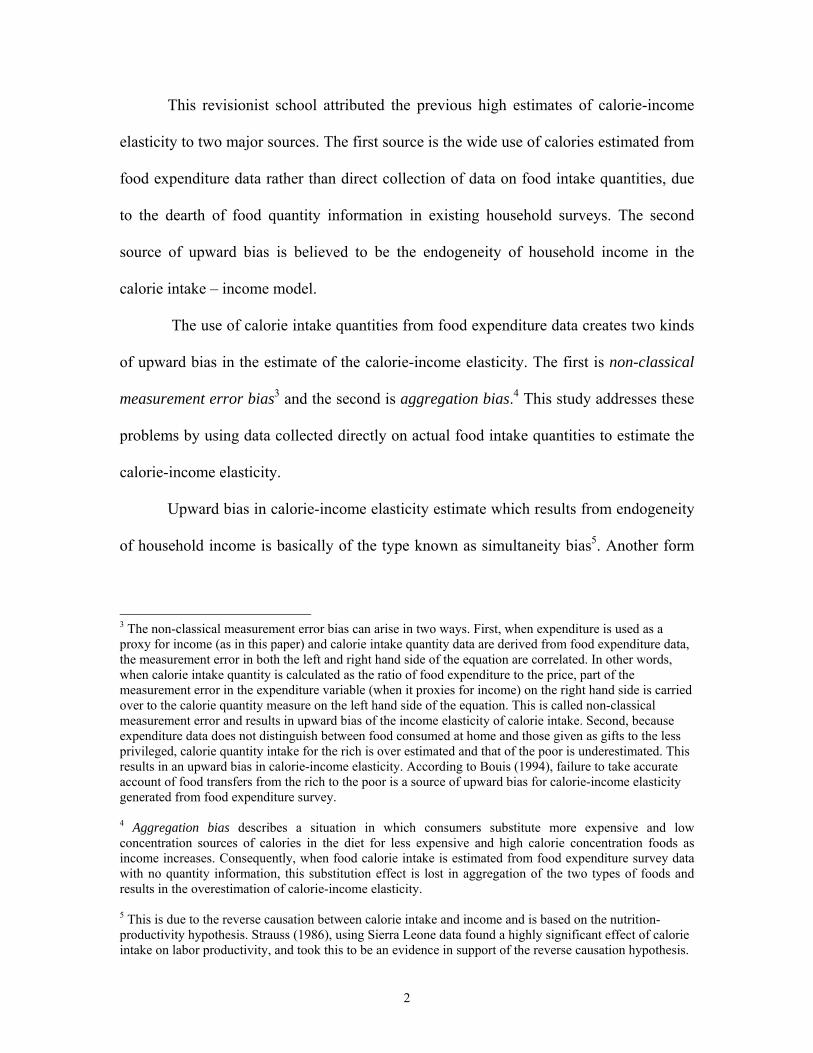
This revisionist school attributed the previous high estimates of calorie-income

elasticity to two major sources. The first source is the wide use of calories estimated from

food expenditure data rather than direct collection of data on food intake quantities, due

to the dearth of food quantity information in existing household surveys. The second

source of upward bias is believed to be the endogeneity of household income in the

calorie intake – income model.

The use of calorie intake quantities from food expenditure data creates two kinds

of upward bias in the estimate of the calorie-income elasticity. The first is non-classical

measurement error bias3 and the second is aggregation bias.4 This study addresses these

problems by using data collected directly on actual food intake quantities to estimate the

calorie-income elasticity.

Upward bias in calorie-income elasticity estimate which results from endogeneity

of household income is basically of the type known as simultaneity bias5. Another form

3 The non-classical measurement error bias can arise in two ways. First, when expenditure is used as a proxy for income (as in this paper) and calorie intake quantity data are derived from food expenditure data, the measurement error in both the left and right hand side of the equation are correlated. In other words, when calorie intake quantity is calculated as the ratio of food expenditure to the price, part of the measurement error in the expenditure variable (when it proxies for income) on the right hand side is carried over to the calorie quantity measure on the left hand side of the equation. This is called non-classical measurement error and results in upward bias of the income elasticity of calorie intake. Second, because expenditure data does not distinguish between food consumed at home and those given as gifts to the less privileged, calorie quantity intake for the rich is over estimated and that of the poor is underestimated. This results in an upward bias in calorie-income elasticity. According to Bouis (1994), failure to take accurate account of food transfers from the rich to the poor is a source of upward bias for calorie-income elasticity generated from food expenditure survey. 4 Aggregation bias describes a situation in which consumers substitute more expensive and low concentration sources of calories in the diet for less expensive and high calorie concentration foods as income increases. Consequently, when food calorie intake is estimated from food expenditure survey data with no quantity information, this substitution effect is lost in aggregation of the two types of foods and results in the overestimation of calorie-income elasticity. 5 This is due to the reverse causation between calorie intake and income and is based on the nutrition-productivity hypothesis. Strauss (1986), using Sierra Leone data found a highly significant effect of calorie intake on labor productivity, and took this to be an evidence in support of the reverse causation hypothesis.

3

of bias that results from endogeneity of income is the omitted variable bias.6 The sign of

this bias is however dependent the nature of relationship between income and the

dominant source of bias.7 In this study, I adopt the instrumental variable technique to

address this problem of endogeneity of income.

On the other hand, the conventional school of thought which support the

traditional view that calorie-income elasticities are sizeable at least among low income

households argue that recent low estimates of calorie-income elasticity in households

could arise from two sources. First is the frequent use of current income as a measure of

wealth rather than permanent income (Behrman and Deolalikar, 1990)8, while the second

is measurement error in income and expenditure. A major problem associated with data

collected in developing countries is the difficulty in obtaining accurate data on income

and expenditure.9 Both the use of current income and measurement error in the data

6 This bias arises because labor income is a choice variable in the household decision model that allows for labor supply/leisure choices. If both labor supply and consumption decisions are driven by same unobserved factor such as ‘taste for work’, then some proportion of the estimated effect of income on calorie intake may be the result of spurious correlations between calorie intake and income rather than the evidence of a causative effect from income to calorie intake. 7 For example, Wolfe and Behrman (1983) attributed the higher estimate of calorie income elasticities in rural relative to urban areas obtained by Ward and Sanders (1980) to the fact that omitted price variables are likely to be correlated with the location variable, resulting in an upward bias of the rural calorie income elasticity. 8 The reasons for this are twofold: First, current income is a very noisy measure of the wealth flow into a household and this enlarges the value in the denominator of the regression coefficient estimator. Second, the covariance between current income and food consumption is believed to be lower than that between permanent income and food consumption (permanent income hypothesis). Thus if current income is used, the numerator of the regression coefficient estimator is understated. The interaction of these two effects would lead to a downward bias in the estimate of the regression coefficient of income in the food calorie intake equation. 9 Two major reasons for this are: the disproportionately large informal sector with little or no formal income records, and the general view that detailed information on personal income is private and that this privacy should be protected from second parties including members of the same household.

4

would bias the ordinary least square regression estimate of the calorie-income elasticity

downwards. 10

Per-capita expenditure is therefore used in place of current income in this study

since it is a better proxy for permanent income. Furthermore, the use of per capita

expenditure as proxy for income reduces measurement error in income since it is easier to

get information on expenditures than on income in developing countries. To further

reduce the magnitude of error, I used income, expenditure and daily calorie intake values

which are averages over 12 fortnightly visits to each sample household.

The second point of investigation in this study is the effect of women’s share of

income on calorie intake in low income households. Studies that investigate the effect of

variation in household resource control pattern on household investment and

consumption patterns in developing countries are not common, due to the dearth of

gender disaggregated household level information on income, expenditure and

consumption. No such study is available for Nigeria.

Hopkins et al (1994) found that in Niger that changes in female annual income,

while controlling for male income impacted positively on household food expenditures.

These results, they claim, hold for both earned and non-labor income. Hoddinott and

Haddad (1995), using data from Cote De ‘Ivoire found a positive but small marginal

effect of women’s income share on household food budget share. A doubling of the

proportion of household cash income received by wives would lead to a meagre 1.9 %

rise in budget share of food eaten within the household. Thomas (1997) on the other hand

found in his analysis of Brazilian data that the marginal effect of increasing women’s

income on food expenditure share is negative and higher than the marginal effect of

10 This bias is called the classical measurement error bias or attenuation bias.

5

husband’s income. He also found that household food calorie intake, protein intake,

height-for-age and weight-for-height of children intake responds more positively to

increases in women’s income than to increases in husband’s income. He concludes that

the identity of the identity of the household member controlling income (non-labor or

total) affects calorie intake, protein intake, height-for-age of children, and weight-for-

height of children.

On the whole, the observed impact of women’s income share on household

consumption and investment patterns is thought to be a reflection of gender differentiated

preferences. The analysis in this paper in based on household consumption, income, and

expenditure data disaggregated by gender and thus gives us a rare opportunity to examine

the effect of variation resource control pattern on per capita calorie intake. This paper

hopes to contribute to the growing literature on determinants of calorie intake at the

household level by investigating the response of calorie intake of individuals in the

household to increases in both per capita expenditure and the share of household income

controlled by women. The model estimated in this paper also allows for differential

income responses for individuals, taking account of the effect of age and sex11.

The major findings of this study are as follows. First, expenditure elasticity of per

capita calorie intake is estimated to be between 0.00 and 4.00 percent, suggesting that

calorie intake does not get a substantial share of marginal increases in household income.

Thus, increasing household disposable income may not be a very effective strategy for

bringing about increased food energy intake among low income populations in Nigeria.

11 Behrman and Deolalikar (1990) observed that not many existing studies have used individual level data to examine calorie- income response relationships as used in this paper. (Behrman and Deolalikar , 1990)

6

Second, we find some support for the Engel proposition that expenditure elasticity

varies inversely with income level, in the ordinary least square estimate of the calorie-

expenditure function. Log per capita expenditure entering either singly or in conjunction

with its quadratic term was not statistically significant under the Instrumental variable

two stage least square technique. (IV-2SLS)

Third, I estimate women’s share of income elasticity of per capita calorie intake to

be between -0.02 and –0.05 and show that this negative marginal response is neither a

consequence reallocation of income towards more expensive and low calorie food

sources nor an evidence of positive transaction cost resulting from imperfect substitution

between male and female income in food consumption. This estimate is a rejection of the

hypothesis that per capita calorie intake is positively related to increasing women’s share

of household income and suggests that wealth redistribution from men to women would

not increase per capita food energy intake in low income households in rural south

western Nigeria.

Finally, it is observed that the OLS and 2SLS estimates of women share of

income are both negative, showing some consistency in the sign attached to the

coefficient of women’s income share variable irrespective of type of estimator (i.e. OLS

or 2SLS).

2.0 IMPORTANCE OF FOOD CALORIE INTAKE

Economic analysis of calorie consumption by households derives from the

important role calories play in the definition of important welfare concepts such as health

7

and labor productivity12. According to Maxwell and Frankeberger (1992), enough food is

mostly defined with emphasis on calorie and on requirements for an active, healthy life

rather than simple survival. 13

Food calorie intake has been found to have a strong empirical linkage with both

human health and productivity. The human body needs energy to maintain normal body

function (basic metabolic rate), engage in required minimal activity related to good health

and hygiene (standard minimum requirement), and carry out productive activities to

sustain the supply of energy and other required nutrients to the body. The level of calorie

intake (both stock and flow) by an individual should therefore be adequate to sustain

these functions over his expected lifetime. When this lifetime calorie consumption

pattern falls short of a minimum threshold, the individual is at a health risk. Secondly

whenever there is a persistent short fall in the flow of calorie intake relative to the amount

required for optimal productive activity, the inflow of other nutrient intakes is likely to be

affected since the resources required to acquire these nutrients is obtained from

productive work. This situation is especially true in populations where the major income-

earning asset is human labor efforts, as is investigated in this study. That is, populations

made up of poor households where non-earned income forms an insignificant component

of full income. In such populations, increased calorie intake may imply increased

productivity, increased income and thus improved overall nutrition.14 Increased nutrition

12 See Stiglitz (1976) for a detailed discussion of the efficiency wage hypothesis which provides the theoretical framework for understanding the link between productivity and calorie intake. 13 Food energy requirements are often used as proxy for all nutritional requirements, even though adequacy in calories may occur simultaneously with serious deficiencies in other nutrients. 14 Using household level data from Sierra Leone, Strauss (1986) found highly significant effect of calorie intake on labor productivity.

8

is associated with sustained increments in productivity and thus sustained access to food

energy intake.

3.0 THEORETICAL FRAMEWORK

The analysis in this paper is approached from the point of view of a cooperative

bargaining household model. There are two general classes of household models namely:

income pooling and bargaining models. The income pooling models assume that

household demand (or expenditure share) is not affected by the identity of the individual

that earns the income. The effective constraint on the household welfare function is the

pooled household income. On the other hand, the bargaining model throws away the

income pooling assumption of the income pooling models and allows for the explicit

effect of distributional factors on demand or expenditure share.

Income pooling models are of two types – unitary or common preference models

and collective or individual preference models of the household. The unitary model

(which is a restricted form of income pooling models) assumes that the preferences of

household members are uniform or that the preference of just one household member (the

household head or dictator) is imposed on all other members. The unitary household thus

maximizes a welfare function whose only component is the utility function of the dictator

or household head. On the other hand, the collective model allows for a more general

formulation of the household welfare function while still accommodating income the

pooling restriction. Unlike in the unitary model, it allows for differences in preferences

between actors within the household.

In the set of collective or individual preference models, household welfare

function is defined as:

9

I Uh = Σ Φi Ui ; i = 1 …….I (3.1) i=1 and Φi = K

where Uh is the household welfare function, Ui is individual i’s utility function

in a household with I individuals. Φi is the welfare or Pareto weight attached to the utility

function of each individual I and K is a vector of constants with i elements whose values

range between 0 and 1. By characterization of this model, Φi is fixed and does not change

with changes in factors that affect resource control power (also called distributional

factors) within the household such as individual income, assets, and schooling. Thus,

changes in distributional factors do not affect the relative expenditure share on goods in a

collective model. It is assumed that Φi is set from marriage and does not change

throughout the life time of the household. So the collective model results in a demand

system derived from a Pareto optimal allocation with a fixed Φi vector. There is no

movement along the utility possibility frontier of the household, since only one point on

the contract curve is relevant.15 The predictions of the collective model is that income

changes only affect household demand directly through the Slutsky income effect and not

through the power sharing factor in the household welfare function. The unitary model is

a special case of the collective model where Φi = [1,0], given that i = 2.

The second broad class of household models is the non-income pooling or

bargaining model. This is the model that is assumed for the analysis carried out in this

paper. The bargaining model jettison the income pooling assumption of the collective

model and allows for the explicit effect of distributional factors on household demand or

15 The contract curve is a locus of Pareto optimal allocations for the household.

10

expenditure levels. The model specifically assumes that Φi ≠ [1, 0] and that Φi ≠ K.

Thus, the whole range of utility possibility frontier is the set of feasible Pareto optimal

allocations for the decision making environment characterized by bargaining. In this

model, changes in power sharing or distributional factors are expected to lead to changes

in Φi and the changes in Φi are in turn expected to result in changing demand pattern or

expenditure shares. Thus, the bargaining model predicts that income changes affect

demand both directly (through the Slutsky income effect) and indirectly (through the

power sharing factor, Φi ).

Assume that a household in this study is made up of a man (m), a woman (f), and

others members who are non-income earners (c); individuals in the household have

differentiated preferences; and household income is not pooled. Suppose that the each

individual in the household derive utility from two composite good: calorie/energy

producing good, C, and non-calorie producing goods, Q. Calorie itself cannot be

purchased but its intake depends on the amount of food item Xj consumed. The amount of

food item, Xj, consumed in turn depends on its price, Pj, and a number of tastes factors

such as characteristics of the individual (γi) and household level characteristics (γh). We

assume that the pareto/welfare weights of the man, Φm , and the woman, Φf , sum to unity,

implying that other members of the household, (c), who have no bargaining power have

pareto weights Φc = 0. Also the household income, Yh, is the sum of the individual

incomes of the man, Ym, and the woman, Yf. Given a particular level of household

income, higher levels of Yf would imply higher bargaining power for the woman or

higher Φf. Thus Φf is a function of the distributional /power sharing factor Yf/Yh.

The household solves the maximization problem stated in expressions 3.2 to 3.7:

11

Maximize Uh = Φm Um ( C, Q) + Φf Uf (C , Q) (3.2) Subject to: Yh = pjXj + Q (3.3) Yh = Ym + Yf (3.4) C = C ( Xj, γi, γh ) (3.5) Φi

≠ K; where K is a constant and i = (m, f) (3.6) Φf = Φf (Yf /Yh), and Φm = (1- Φf ) (3.7).

From this constrained maximization problem, we derive an optimal demand

function for calorie intake as a function of prices, household income, a power sharing or

distributional factor, individual and household level characteristics. Formally,

C = C (Xj(p), Yh, Φf (Yf /Yh), γi, γh) (3.8)

4.0 DATA

4.1 Data Collection Procedure

Three states were selected out of the six states in South-western Nigeria. The

three states selected are Ogun representing the Lagos/Ogun group; Oyo representing the

Oyo/Osun group and Ondo representing the Ekiti/Ondo group. Historically, the three

groups are more homogeneous within than between in terms of culture and tradition.

Four rural local government areas were selected in each of Ogun, Ondo and Oyo

states. There are 3 main geopolitical divisions in each state called Senatorial Districts.

Each senatorial district is in turn made up of Local Government Areas (LGAs). At least

one L.G.A. was selected from the list of rural LGAs in each of the 3 senatorial districts in

each state. The Headquarters of the selected rural local government areas were

automatically selected for the survey. The headquarters were selected since the

12

population in the headquarters is assumed to represent the best mix of the dwellers in the

L.G.A. It will also allow the sampled households to exhibit enough variability in the

major variables of concern in the study. A total of 12 LGAs were selected in all. The

selected local government areas are as shown in Table 1. They are, Egbado-North,

Obafemi-Owode, Remo-North and Ijebu-East from Ogun State; Ibarapa-North, Itesiwaju,

Surulere and Saki-East from Oyo; and, Irele, Ondo-East, Akure-North and Akoko-North-

West from Ondo State. All the selected local government headquarters can be classified

either rural or semi-urban. None can be classified as urban.

A combination of cluster and systematic random sampling was used to select 40

households from each of the selected 12 rural/semi-urban communities. Thus, a total of

160 households per state and 480 households in all were selected.16 However, the

analysis used information from only 472 households, amounting to 2573 individuals who

16 One major requirement for the choice of Field Assistants for was that they must have been resident in the community for an appreciably long time and must be acceptable to the people. Before the commencement of operations in each LGA, the local government office, Traditional Rulers, and other popular community leaders were contacted for official permission and moral support during the period of the study. They were in the process intimated with the importance of the study. Letters of recommendation were obtained from the council office to give official backing to the study. Each selected community was divided into 4 clusters. Each cluster consisted of residential areas nearest to one another. From the list of major residential areas under each of the 4 clusters, one area is chosen by a simple random procedure. The lists of streets under each of the 4 selected residential areas were compiled and 2 streets were chosen by simple random sampling procedure. 5 houses were chosen from each of the 2 streets selected from each area. This was done by a systematic random sampling, using the random number table. A listing of the houses in the selected streets was made to get the approximate number of houses in the street. Let us assume that the number of the houses listed in the street is 50 houses and we want to pick 2 houses in the street. Our population (N) = 50 and our sample size (n) = 2. We calculate a sampling interval (S.I ) of 25 through the formula: S.I. = N/n = 50/2 = 25. The random number table (RNT) was then used to get the random start (R.S). Random start (R.S.) is the first house to be picked in the community. The R.S. must not be greater than the S.I. It is either less than or equal to the S.I. 5 houses were chosen at the interval of the sample interval (S.I), 25. The 5 houses selected through the systematic procedure were then visited to make a list of the number of households. One household is then chosen by a simple random procedure if more than one household dwell in a selected housing unit. The total number of households selected was thus 10 for each of 4 areas, in each of 4 communities, in each of 3 States. The researchers then called on the head of the chosen household to introduce themselves and seek permission to conduct the study for six months. Efforts were made to obtain the full permission of the household head and cooperation of all household members. The list of the consenting households was subsequently made. (see Aromolaran, 2001.)

13

are at least 2 years of age (See Table 1).17 The needed information was collected through

the use of interview schedules/questionnaires that were personally administered by the

field assistants and field supervisors. Food price data were obtained through community

market surveys. 18

Food consumption information was collected on individual basis from the

households. Quantities of daily food intake were collected for each member of the

household, using a 48-hour recall method.19 Each household was visited at least once in

two weeks. Data were collected over a period of 6 months (October 1999 – March 2000).

Thus daily food intake quantities for each individual in the household were collected two

times every month for a total of twelve times in 6 months. The analysis reported here

was based on per capita daily food consumption averaged over the 6 months of data

collection. This is designed to reduce measurement error in food consumption by

smoothening day-to-day fluctuations in food intake. These quantities were then converted

into kilogram units. The daily calorie intake level of the individual Ci , was computed

through the formula:

m

Ci = Σ ωj Fij (4.1)

j = 1

17 Children below 2 years were not considered in the analysis because many of them were still being breast-fed. 18 Consequently, food prices only vary across the 12 local government areas. 19 Individuals were asked about the amount of food they consumed in the last 24 hours, and then in the preceding 24 hours. There was no direct weighing of food quantities. The method used to obtain the measure of food quantities was indirect. A standard size of each major food item was prepared and weighed at the research office. These physical measures were taken as the unit of measurement on the field. Each survey personnel carried the physical measures with them and used them to assist the individuals in assessing the quantities of food items taken in the past 48 hours. For example, if one respondent says he consumed twice the field unit for a particular food item, then his intake of that item in kilograms will be the weight of the standardized field unit multiplied by 2.

14

Where: Fij is the weight in grams of the average daily intake of food commodity j

by individual i. ωj is the standard measure of calorie found in each type of food

commodity Fj . A total of 46 food items that were considered common food items in the

area constituted our basket of food.20 (i.e J=46).

Income from different occupational sources was obtained on a fortnightly basis

for a period of six months. No distinction was made between labor and non-labor income

in the computation of the income variable used in this analysis 21 and all income data

were collected from each income-earning members of the household. Expenditure

information by item was also collected every two weeks for each income-earning

member of the household.22

4.2 Food Consumption Pattern and Calorie Intake in South Western Nigeria

According to FAO (1985), food consumption pattern is measured by the share of

dietary energy supplies contributed by each major food group. The analysis under this

subsection involved the computation of the percentage contribution of each major food

group in the food basket of the households in the study area to total calorie intake. It

20 The food items include Yam, Pounded Yam, Asaro (Mashed Yam Meal), Amala Isu (Dried Yam Dough) , Gari (fried fermented cassava granules), Eba (dough made from Gari), Fufu (Wet Cassava Flour Dough), Amala Lafun (dried cassava flour dough), Boiled Beans, Moinmoin ( boiled bean dough) Akara ( fried bean dough) , Boiled Rice, Ogi ( Liquid Maize Pap), Eko ( Solid Maize Pap) , Boiled Maize, Potatoes, Butter, Milk, Tea/coffee, Sugar, Beverages (e.g.Bournvita, Milo) Plantain/Dodo, Bread, Biscuit/snacks, Vegetables, Pomo (Cow Skin), Beef , Pork, Sheep/Goat Meat, Chicken, Eggs, Fish, Orange, Pawpaw, Banana, Vegetable,Oil , Pepper/Tomato, Palm Oil, Gari, Cocoyam, Melon, Okro, Groundnut, Cray Fish, Snail, Games (Bush Meat), Elubo Isu (yam flour).

21 Given the possibility of reverse causality between calorie intake and labor income, the use of non-labor income instead of the sum of both labor and non-labor income on the right hand side would have been a good idea. However, this could not be done in this case because of non-availability of separate useable data on non-labor income. 22 This implies that all consumption expenditures in the household were fully assigned to income earning members. For example if a teenage daughter who earns no income bought some cloths, the amount spent on the cloths is assigned to the income earning household member who transferred the amount to her.

15

shows the importance of each food item in the food calorie basket of the average

individual in the study area.

Table 2 reveals that food consumption pattern is essentially the same among

males and females, with roots and tubers supplying close to 60 percent of calorie intake.23

Cereals provide only 17 percent of calorie intake while legumes contribute 7 percent.

Less than 3 percent of energy intake comes from animal products, while oils and fats

provide 10-11 percent. This food consumption pattern is a fair reflection of the farming

patterns in the study area since roots and tubers are the dominant food crops followed by

cereals and oil palm. The finding that low quality high carbohydrate foods are the major

source of calories is an indication that adequate calorie intake may not imply adequate

intake of other nutrients in the study area.

Table 3 shows that adults get a greater proportion of their calorie intakes from

cereals, legumes and animal products than children do. On the other hand, children below

the age of 6 years get 60 percent of the energy intake from roots and tubers alone, while

adults get about 53 percent. Thus, children below the age of 10 years obtain

proportionately more calories from low quality foods than adults. This has important

implications for child welfare.

Table 4 shows that age is a very important determinant of the level of calorie

intake. For both males and females average daily calorie intake increases with age.

Secondly, children and adolescents, particularly males, do not consume enough calories

to meet their daily minimum energy requirements. Even though, in absolute terms, males

consume slightly more calories than females, calorie intake deficiency is more profound

23 Roots and tubers are high carbohydrate foods which contain insignificant amounts of other nutrients apart from calories.

16

among males than females because of the lower minimum energy requirement by

females.

The numbers in the first panel of Table 5 imply that per-capita daily calorie

intake does not vary with formal educational status of household head, while the second

panel shows that calorie intake is higher across age groups for individuals in households

whose major source of income are the food sector compared with households who obtain

most of their incomes from non-food related sources.

4.3 Socio-economic Characteristics of Households

From Table 6, we observe that average calorie intake per capita is 2204

kilocalories and note that this is below the 2500 kcal recommended by FAO as standard

minimum daily requirement. This shortfall of 13.4 percent substantially understates the

energy deficiency problem given the fact that poor families generated virtually all their

incomes through direct labor efforts. Per capita consumption expenditure is estimated as

2135 Naira per month (or $US26).24 Furthermore it is estimated that 57.4 percent of total

value of food consumed at home is purchased from the market. The implicit cost of 1000

units of calories is 28.8 Naira ($0.36). Total asset possessed by the average household is

valued as 810,506 Naira (or $US10,131), with a median value of 342,570 Naira ($4280).

The average household size in the sample consists of 7 persons. 12 percent of

household heads and 8 percent of senior wives have some tertiary education, while 44

percent of household heads and 48 percent of senior wives have no formal education. The

average husband in the study area has 5.1 years of schooling while the average senior

24 The public service minimum wage at the time of data collection was 3000 Naira.

17

wife has 4.3 years of schooling. Thus the ratio of years of schooling of wife to the

husband in the average household is 0.80.

Table 2 further shows that women’s share of household income is about 0.353 and

women’s share of total household food expenditure is 0.321 percent. We also observe

that the food share in total women’s consumption expenditure is 0.32, indicating that

women spend more of their income on non-food consumption items. 25 Women’s share

of own-farm produce consumed at home is 0.0736, showing that men supply most of the

farm produce consumed at home. Women’s ownership share of total acreage farmed is

only 0.144.26 Furthermore, while women’s share of total farmland value is just 7 percent,

women’s share of business assets is about 0.304, implying a lower involvement of

women in farming compared with non-farm businesses. This is supported by the fact that

while 59 percent of household heads earn their income mainly from non-farm sources; 70

percent of senior wives earn their income mainly from this source. 27

25 Incomes earned were recorded separately for men and women. Expenditures made by men and women were also recorded separately. Both income and expenditure measures included farm produce consumed at home. Home production of non-marketable goods and services are not accounted for as a form of income and expenditure. This would certainly understate the full income of the household and may understate the income of wives relative to husbands. To avoid double counting, only expenditures made from own-income were recorded for an individual. For example a woman may expend 100 units of money on consumption during the month. If 80 percent of it were transfers from her husband, then her own expenditure is just 20 units of money. 26 Not all plots are individually owned, since we have both individual and family farms. Yet all plots could be easily assigned to either the husband or the wife. All family farms are assigned to the household head (who are in 88% of the time males). This is because the men fully control the incomes and expenditure from these farms. Plots assigned to women are those that belong solely to the women; plots upon which they exercise a dominating control over income and expenditure patterns. 27 About 23 percent of household heads and 9 percent of senior wives are wage earners.

18

5.0 EMPIRICAL MODEL

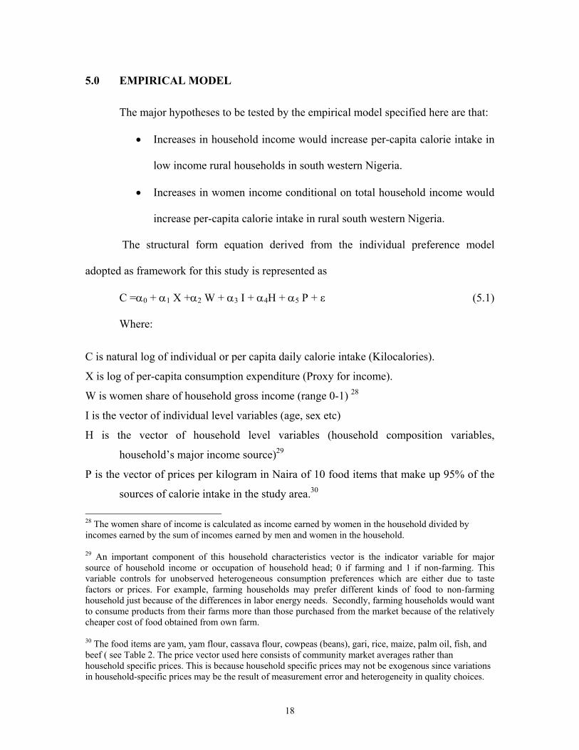
The major hypotheses to be tested by the empirical model specified here are that:

• Increases in household income would increase per-capita calorie intake in

low income rural households in south western Nigeria.

• Increases in women income conditional on total household income would

increase per-capita calorie intake in rural south western Nigeria.

The structural form equation derived from the individual preference model

adopted as framework for this study is represented as

C =α0 + α1 X +α2 W + α3 I + α4H + α5 P + ε (5.1) Where:

C is natural log of individual or per capita daily calorie intake (Kilocalories).

X is log of per-capita consumption expenditure (Proxy for income).

W is women share of household gross income (range 0-1) 28

I is the vector of individual level variables (age, sex etc)

H is the vector of household level variables (household composition variables,

household’s major income source)29

P is the vector of prices per kilogram in Naira of 10 food items that make up 95% of the

sources of calorie intake in the study area.30

28 The women share of income is calculated as income earned by women in the household divided by incomes earned by the sum of incomes earned by men and women in the household. 29 An important component of this household characteristics vector is the indicator variable for major source of household income or occupation of household head; 0 if farming and 1 if non-farming. This variable controls for unobserved heterogeneous consumption preferences which are either due to taste factors or prices. For example, farming households may prefer different kinds of food to non-farming household just because of the differences in labor energy needs. Secondly, farming households would want to consume products from their farms more than those purchased from the market because of the relatively cheaper cost of food obtained from own farm. 30 The food items are yam, yam flour, cassava flour, cowpeas (beans), gari, rice, maize, palm oil, fish, and beef ( see Table 2. The price vector used here consists of community market averages rather than household specific prices. This is because household specific prices may not be exogenous since variations in household-specific prices may be the result of measurement error and heterogeneity in quality choices.

19

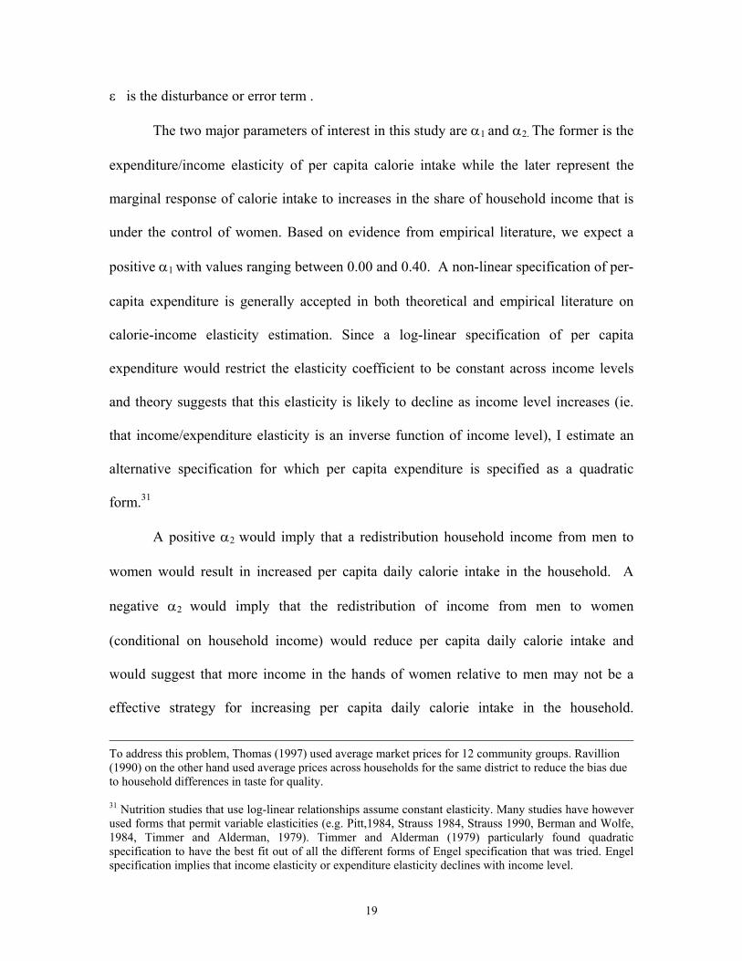
ε is the disturbance or error term .

The two major parameters of interest in this study are α1 and α2. The former is the

expenditure/income elasticity of per capita calorie intake while the later represent the

marginal response of calorie intake to increases in the share of household income that is

under the control of women. Based on evidence from empirical literature, we expect a

positive α1 with values ranging between 0.00 and 0.40. A non-linear specification of per-

capita expenditure is generally accepted in both theoretical and empirical literature on

calorie-income elasticity estimation. Since a log-linear specification of per capita

expenditure would restrict the elasticity coefficient to be constant across income levels

and theory suggests that this elasticity is likely to decline as income level increases (ie.

that income/expenditure elasticity is an inverse function of income level), I estimate an

alternative specification for which per capita expenditure is specified as a quadratic

form.31

A positive α2 would imply that a redistribution household income from men to

women would result in increased per capita daily calorie intake in the household. A

negative α2 would imply that the redistribution of income from men to women

(conditional on household income) would reduce per capita daily calorie intake and

would suggest that more income in the hands of women relative to men may not be a

effective strategy for increasing per capita daily calorie intake in the household.

To address this problem, Thomas (1997) used average market prices for 12 community groups. Ravillion (1990) on the other hand used average prices across households for the same district to reduce the bias due to household differences in taste for quality. 31 Nutrition studies that use log-linear relationships assume constant elasticity. Many studies have however used forms that permit variable elasticities (e.g. Pitt,1984, Strauss 1984, Strauss 1990, Berman and Wolfe, 1984, Timmer and Alderman, 1979). Timmer and Alderman (1979) particularly found quadratic specification to have the best fit out of all the different forms of Engel specification that was tried. Engel specification implies that income elasticity or expenditure elasticity declines with income level.

20

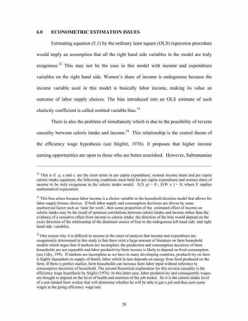
6.0 ECONOMETRIC ESTIMATION ISSUES

Estimating equation (5.1) by the ordinary least square (OLS) regression procedure

would imply an assumption that all the right hand side variables in the model are truly

exogenous.32 This may not be the case in this model with income and expenditure

variables on the right hand side. Women’s share of income is endogenous because the

income variable used in this model is basically labor income, making its value an

outcome of labor supply choices. The bias introduced into an OLS estimate of such

elasticity coefficient is called omitted variable bias.33

There is also the problem of simultaneity which is due to the possibility of reverse

causality between calorie intake and income.34 This relationship is the central theme of

the efficiency wage hypothesis (see Stiglitz, 1976). It proposes that higher income

earning opportunities are open to those who are better nourished. However, Subramanian

32 That is if µ, υ and ε are the error terms in per capita expenditure, women income share and per capita calorie intake equations, the following conditions must hold for per capita expenditure and women share of income to be truly exogenous in the calorie intake model: E(X µ) = 0 ; E(W υ ) = 0; where E implies mathematical expectation. 33 This bias arises because labor income is a choice variable in the household decision model that allows for labor supply/leisure choices. If both labor supply and consumption decisions are driven by same unobserved factor such as ‘taste for work’, then some proportion of the estimated effect of income on calorie intake may be the result of spurious correlations between calorie intake and income rather than the evidence of a causative effect from income to calorie intake. the direction of the bias would depend on the exact direction of the relationship of the dominant source of bias to the endogenous left hand side and right hand side variables. 34 One reason why it is difficult to assume at the onset of analysis that income and expenditure are exogenously determined in this study is that there exist a large amount of literature on farm household models which argue that if markets are incomplete, the production and consumption decisions of farm households are not separable and labor productivity/farm income is likely to depend on food consumption (see Udry, 199). If markets are incomplete as we have in many developing countries, productivity on farm is highly dependent on supply of family labor which in turn depends on energy from food produced on the farm. If there is perfect market, farm households can increase farm labor input without reference to consumption decisions of household. The second theoretical explanation for this reverse causality is the efficiency wage hypothesis by Stigliz (1976). In this latter case, labor productivity and consequently wages are thought to depend on the level of health and nutrition of the job seeker. So it is the calorie intake level of a non-landed farm worker that will determine whether he will be able to get a job and thus earn some wages at the going efficiency wage rate.

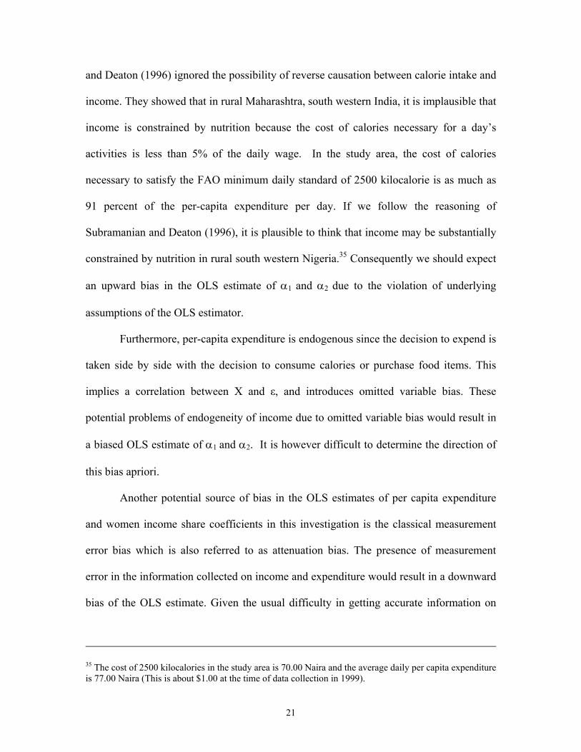
21

and Deaton (1996) ignored the possibility of reverse causation between calorie intake and

income. They showed that in rural Maharashtra, south western India, it is implausible that

income is constrained by nutrition because the cost of calories necessary for a day’s

activities is less than 5% of the daily wage. In the study area, the cost of calories

necessary to satisfy the FAO minimum daily standard of 2500 kilocalorie is as much as

91 percent of the per-capita expenditure per day. If we follow the reasoning of

Subramanian and Deaton (1996), it is plausible to think that income may be substantially

constrained by nutrition in rural south western Nigeria.35 Consequently we should expect

an upward bias in the OLS estimate of α1 and α2 due to the violation of underlying

assumptions of the OLS estimator.

Furthermore, per-capita expenditure is endogenous since the decision to expend is

taken side by side with the decision to consume calories or purchase food items. This

implies a correlation between X and ε, and introduces omitted variable bias. These

potential problems of endogeneity of income due to omitted variable bias would result in

a biased OLS estimate of α1 and α2. It is however difficult to determine the direction of

this bias apriori.

Another potential source of bias in the OLS estimates of per capita expenditure

and women income share coefficients in this investigation is the classical measurement

error bias which is also referred to as attenuation bias. The presence of measurement

error in the information collected on income and expenditure would result in a downward

bias of the OLS estimate. Given the usual difficulty in getting accurate information on

35 The cost of 2500 kilocalories in the study area is 70.00 Naira and the average daily per capita expenditure is 77.00 Naira (This is about $1.00 at the time of data collection in 1999).

22

income and expenditure of individuals and households in developing countries,

measurement error bias may be a very important source of bias in this study.

Attempts made in this study to reduce the effect of these potential sources of bias

on the estimate of per capita expenditure and women’s income share elasticity can be

categorized into two. First are measures taken at the data collection stage, and second are

measures taken at the estimation stage. Figures on food intake, income and expenditure

used in the analysis are averages of data collected through multiple visits over a period of

six months. This is expected to reduce classical measurement error since we use the mean

of the distribution of quantities/values for each respondent over a period of time. Second,

data on calorie intake was obtained directly from food quantity data and not indirectly

from food expenditure data. This reduces the potential upward bias from non-classical

measurement errors.36 Third, values of time varying and time invariant assets of the

household and individuals were collected at the beginning and end of the survey. The

average values were used in the analysis.

The instrumental variable two stage least square (2SLS) estimation procedure is

used to address the problems relating to measurement error bias, simultaneity and

endogeneity of income/expenditure. With this procedure, expression 6.1 is estimated in

place of expression 5.1.

C = β0 + β1 X* + β2 W* + β3 I + β4H + β5 P + ε* (6.1)

Where

36 This non-classical measurement error is created if calorie intake quantity is computed from food expenditure data. In such cases, any measurement error in the expenditure on the right hand side is carried on to the calorie intake value on the left hand side. As a result the estimated coefficient of per-capita expenditure would potentially have an upward bias.

23

X* and W* are predicted values of the two endogenous explanatory variables and

ε* is an error term that is uncorrelated with X* and W*. To obtain X* W* and ε*,

expressions 6.2 and 6.3, called first stage regression equations are estimated.

X = δ0 + δ1 I + δ2 H + δ3 P + δ4 Z + µ (6.2)

Ws = Φ0 + Φ1 I + Φ2 H + Φ3 P + Φ4 Z + υ (6.3)

Where I, H, and P are as defined in expression 5.1 and Z is the 1xK vector of

identifying instruments. Both µ and υ are assumed to be well behaved (i.e. independently

and identically distributed, i.i.d.) with mean zero and constant variance, and X* = X – µ,

while W* = W – υ.

For the set of instruments used in this study to be valid, δ4 and Φ4 would have to

be identified. That is the following conditions must hold for each equation.

E( Z X) ≠ 0 ; E( Z W) ≠ 0; (6.4)

E (C Z / X, W) = 0 (6.5),

Where E represents mathematical expectations.

Thus for an instrument to be valid it must be strongly correlated with per capita

expenditure, X, or women’s income share, W (expression 6.4) and should not be

significantly correlated with per capita daily calorie intake when conditioned on per

capital expenditure and women income share (expression 6.5). That is, after controlling

for X and W, the effect of the Z-vector of instruments on per capita calorie intake should

be close to zero.

Four such variables where found and used as instruments for per capita

expenditure and women’s income share in this study.37 These variables are total value of

37 The first task in the estimation was to find strong predictors for the endogenous variables on the right hand side of the specified calorie intake. 4 significant predictors were selected after for both log per capita

24

all household’s assets38, the couple’s total number of years of schooling39, ratio of the

years of schooling of senior woman to the household head, and the share of household

business asset controlled by women. 40

Theoretically both total value of assets and total number of years of schooling is

expected to be a fair indicator of the income earning capacity of the household. That is

we expect per capita consumption expenditure to increase as households become

wealthier in terms of farm and non-farm business asset ownership. Holding the total

value of assets constant, it is expected that increases in women’s share of household

assets would increase per-capita consumption expenditure. Women’s income share is

expected to be predicted by women share of household business asset and the ratio of

women’s years of schooling to that of the household head. That is, as women get control

over more business assets relative to men in the household, we expect their share of

income and women’s share of income after running a series regressions. These are sum of years of schooling of husband and wife, ratio of wife’s years of schooling to husband’s years of schooling, total value household asset, women’s share of household’s business asset. 38 The total value of all household assets is the sum of the value of all business and non-business assets owned by the household. This includes land, farm implements, farm buildings, farm machinery, non-farm business machines and equipments. This estimate does not include farm supplies like fertilizer, seeds chemicals etc or inventories. 39 This is the sum of years of education of husband and senior wife. 40 Hopkins et al (1994), instrumented annual male income with the following variables: land area operated by males, the value of male livestock assets, a dummy variable for male literacy, the number of wives, the dependency ratio, a variable for single or multiple conjugal units within the household, the age of the household head, quadratics of several variables and interaction terms. The annual female income was instrumented using the land area operated by female, the value of female livestock assets, a dummy variable for female literacy, the number of infants in the household, the number of caretakers in the household (girls between the ages of ten and fifteen), a market village dummy, an ethnicity dummy, quadratics of several variables, and interaction terms. The instruments that were used to predict the log of per capita expenditure in Hoddinott and Haddad (1995) and Haddad and Hoddinott (1994) include: the amount of land owned by the household, the logarithm of the per capital value of holdings of consumer durable, the number of rooms per capita in the dwelling, the per capita floor area of the dwelling, and dummy variables equaling one; if the walls of the dwelling are cement, stone or brick; if the floor of the dwelling is cement, stone or brick; if the dwelling is owned by the household and is located in an urban cluster; if the household grows any major internationally traded cash crop.

25

household income to rise. Also, a decline in the schooling gap between household men

and women is expected to lead to an increase in the share of household income under the

control of women.

An important condition for the identification of δ4 and Φ4 in this study is that the

amount of assets owned by the households, total years of schooling of couple, women’s

share of household business asset, and ratio of wife to husband years of schooling would

only affect calorie intake indirectly through their (direct) effect on per capita expenditure

and women’s share of income. If this additional condition is satisfied, then these four

variables would be acceptable as satisfactory identifying instruments for per capita

income and women’s share of income in the calorie intake model.

7.0 RESULTS AND DISCUSSION

7.1 Ordinary Least Square Estimates of Expenditure and Women’s Income Share

Elasticities

Results presented in the first row of the first panel of Table 11 shows a

significant41 ordinary least square (OLS) estimate of per-capita expenditure elasticity of

calorie intake between 0.7 and 3.8 percent. This estimate supports the empirical school

which argues that the response of calorie intake to marginal changes in income is close to

zero (Wolfe and Behrman, 1983, Behrman and Deolalikar, 1987).

The OLS result presented in the third column of Table 9 suggests that expenditure

elasticity of calorie intake is inversely related to income levels. That is calorie intake is

41 The standard errors of the estimated coefficients were corrected for clustering within households by using the robust cluster command in STATA software package. The reason is that the simple estimates of standard errors become incorrect when we have multiple observations, which are not independent within a data. In the data set used for this analysis most of the income and expenditure variables, as well as household head and senior wife characteristics fall into this category of variables. All individuals that

26

likely to respond more to marginal income changes in households located at the lower

percentile of income distribution compared with households located at the higher

percentile. This result is fairly common in empirical literature (Behrman and Wolfe,

1984; Strauss, 1986) although some studies have also found that the log-linear model fits

the calorie intake-expenditure data more satisfactorily (Ward and Sanders 1980, Wolfe

and Behrman, 1983).

We observe from the first panel and first row of Table 11 that a 10 percent

increase in women’s share of household income would result in the lowering of per-

capita daily calorie intake by between 0.15 and 0.19 percent. Even though this negative

effect is small, it is an indication that redistribution of household income from husband to

wife may not be an effective strategy for motivating increasing intake of food calories by

low income rural households in south western Nigeria.

In addition, we observe an insignificant difference between the women’s income

share elasticity estimate from the log-linear expenditure and the non-linear expenditure

calorie intake models. This is an evidence of the robustness of the women share of

income estimate.

7.2 Two Stage Least Square (2SLS) Estimates of Expenditure and Women’s

Income Share Elasticities

As earlier discussed, ordinary least squares estimates of calorie-income and

calorie-women’s income share elasticity are likely to be biased if per-capita expenditure

and income share are endogenous to the calorie intake model. If this assumption of

belong to the same household have the same values for these variables. This is referred to as clustering within households

27

endogeneity of income and expenditure is true, then we would expect that the true

elasticity estimates should be significantly smaller or larger than what the OLS estimate

suggests. On the other hand, if measurement error is considered as a likely dominant

source of bias, then the resulting attenuation bias would imply that the true elasticity

estimates should be higher than what the OLS estimates suggest.

The proposed way of addressing these problems is to use an instrumental variable

(IV) estimator to estimate the coefficients of per-capita expenditure and women’s income

share through a 2SLS procedure. I approach this by first running a first stage regression

to generate reduced form estimates of the endogenous right hand side variables; to show

how well the complete set of instruments predict the endogenous right hand side

variables of the structural model; and to test for the joint significance of the set of

identifying instruments. I then run a second stage regression using all the right hand side

variables in the OLS results discussed above but replacing the observed values of per-

capita expenditure and women’s share of income with the predicted values from the first

stage regression. The results are presented below.

7.2.1 First Stage Regression Results

The results of the first stage regressions for log per-capita expenditure, quadratic of log

per capita expenditure and women’s share of household income are reported in Table 7.

We observe from the F-test results that all the 3 estimated reduced form equations are

statistically significant at 0.000 α-level (see columns 1, 3 & 5 of Table 7). Furthermore,

the set of identifying instruments is able to predict 4.5 percent of the variations in log per-

capita expenditure, 4.6 percent of variations in the quadratic term of log per-capita

expenditure and 23.0 percent of variations in women’s income share ( see columns 2,4 &

28

6 of Table 7). As expected, we observe that the couple’s total years of schooling and the

value of all assets owned by household are significant predictors of log per capita

expenditure. After controlling for these two identifying instruments as well as

wife/husband years of schooling ratio, women’s share of household business assets has

no significant effect on log per capita expenditure, while its effect on women’s share of

income was statistically significant at less than 0.00 percent α-level.42 Women’s share of

household business asset turns out to be the main identifying instrumental variable for

women share of income. That is, after controlling for other model variables, the higher

the proportion of household business assets that belong to women, the higher the

proportion of the household income that is under the control of women.

7.2.2 Second Stage Regression Results and Discussion

The first row of the second panel on Table 11 presents the expenditure and

women’s income share elasticity estimates derived from the 2SLS estimation results

reported in the second panel of Table 9.43

Generally, we find consistency in the sign attached to the estimated coefficient of

per capita expenditure and women’s income share variables irrespective of the type of

estimator (i.e. OLS or 2SLS) or the assumptions about the behavior of expenditure

elasticity vis-à-vis household income level.

42 Women’s share of household income is significantly predicted by all four identifying instrumental variables namely total years of schooling of husband and wife, total value of household assets, wife/husband ratio of years of schooling, and women’s share of household business asset. 43We also observe from Table 9 that individual daily calorie intake is dependent on age of individual with a quadratic form of relationship. Older individuals have higher intakes Calorie intake increases by 2.7 percent from age 2 to 3 and increases at a decreasing rate on till the age of 54.5 years when a decline sets in. The calorie intake level of the farming households is not significantly different from non-farming households. Thus, the occupational status of the household does not exact a significant influence on the level of calorie intake. Finally, males generally had about 4 percent more calorie intakes than females.

29

Per capita expenditure elasticity of calorie intake is estimated to be 3.0 percent

under the linear expenditure model and 0.1 percent under the non-linear expenditure

model. Theoretically, it is expected that income44 increases would enable individuals in

low income households to increase their food calorie intake. This in turn is expected to

improve nutrition status, health and productivity of household members. The observed

low calorie intake elasticity suggests that calorie intake does not get a substantial share of

marginal increases in household income. This result is in line with the conclusion of

Bouis and Haddad (1992) that most recent studies have reported calorie-income elasticity

which are less than 0.2 in contrast to conventional wisdom that calorie-income elasticity

for low income populations in the developing world ranges between 0.4 and 0.8. Thus,

increasing household income may not be a very effective strategy for bringing about

increased food energy intake among low income households in south western Nigeria.45

44 Income is proxied here by consumption expenditure. Consumption expenditure is widely used in place of income because of a number of reasons. One is that it is subject to less errors of measurement and second is that it is a better approximation of permanent income, if we assume that households smooth consumption over their life time. 45 Ravallion (1990) argues that the low calorie income elasticity estimates in literature is counterintuitive and is likely to be the result of data imperfections. He further argues that if this low estimates were a true reflection of reality; it still does not support a conclusion that income increment is not a good policy strategy for reducing under-nutrition. According to him, if we think in terms of head count index of under nutrition, the marginal effect of a change in income of undernourished households on a headcount index of under-nutrition is determined by the product of the calorie income elasticity and the slope of the distribution function of intake. If the distribution function is very steep ( ie a large proportion of the population are just above nutritional adequacy level), a small drop in intake resulting from income changes may move a large proportion of the people below the minimum nutrient intake line. So to assess the impact of income on under-nutrition, we must know the distribution of nutrient intake of the population. That is, we need to know the proportion of households that are close to the minimum nutrient intake line. The more households that are near to this line the more important is income increments in achieving improvements in under-nutrition. He argues that there is a clear difference between the concepts of nutrient intake (which most empirical literature has measured income effect for) and under-nutrition (which involves other factors such as minimum requirement and household and personal characteristics. His major goal in this study are to estimate calorie income elasticity and then use the elasticity estimates to simulate the effects of income changes on various measures of caloric under-nutrition such as head count nutrition index, nutrition deficiency depth index and nutrition deficiency severity index all based on FGT poverty index.

30

These 2SLS expenditure elasticity estimates are larger than the OLS estimates and

are not statistically significant due to larger standard errors.46 In addition, we observe

that the 2SLS of the quadratic term of the log per-capita expenditure variable is not

statistically significant.47

Women’s share of income elasticity estimate is negative and between 3.63 and

5.10 percent, depending on the assumption about the behaviour of per capita expenditure

elasticity as income level increases. Contrary to what we find in the case of per capita

expenditure, these estimates are higher in absolute terms than the corresponding OLS

estimates reported earlier. This may be an indication that classical measurement error

bias is an important source of bias in this investigation since we were unable to

empirically confirm the endogeneity of women’s share of income in this study (see

section 7.3.2 for discussion on the test of endogeneity).48 Both estimates of women’s

share of income elasticity are statistically significant at 5 percent α-level. Thus, a

doubling of the share of household income controlled by women from the current average

of 0.31 to 0.62 will result in a 3.6-5.1 percent decline in per capita calorie intake of the

household from the current average of 2204 kilocalories.

46 The 2SLS estimator is a less efficient estimator compared with the OLS even though the former is more consistent. 47 This statistical insignificance of the quadratic term in the 2SLS estimation in spite of its significance in the OLS estimation may be due to a number of things. First, the assumption may not be true in the population that the income elasticity varies with income levels of households. Second, the data may consist of only households within the same response bracket. Third, the quadratic term of the expenditure variable is not adequately identified. I would think the available evidence supports the third explanation. Table 7 shows that the linear and quadratic terms of the per-capita expenditure variable are not adequately identified. That is there is none of the four identifying instruments that identifies the linear term separately from the quadratic term. 48 Thus even though the use of 2SLS may have resulted in the inability to reject the null hypothesis of zero effect of expenditure on calorie intake due to larger standard error estimates compared with OLS, the higher estimates of elasticity coefficients would suggest that using the 2SLS approach could have at least achieved significant reductions in the effect of classical measurement error bias on elasticity estimates.

31

As implied by the OLS estimates, the 2SLS estimates clearly reject the

hypothesis that per capita calorie intake responds positively to increasing women’s share

of household income, and suggests that income redistribution from men to women would

not increase per capita food energy intake in this population.

However, it can be argued that the observed non-positive response of per capita

calorie intake to changes in women’s share of household income may be evidence of

female preference for more expensive foods with less energy content. To check this, I

estimate the effect of women’s share of income on food calorie price.49 The elasticity

estimates as presented in the second row of the first and second panels of Table 11, show

that the unit cost of calorie consumed does not vary positively with changes in women’s

share of income, suggesting that women do not seem to reallocate expenditures towards

more expensive calorie sources as their income share increase.

Another plausible explanation for the negative sign of the women’s income share

coefficient is the issue of transaction costs. Since the estimate of the effect of women’s

share of income conditions on household income, increasing women’s share of income

would, by definition, be associated with decreasing share for men. Even if household

resources are not reallocated to more expensive foods with less calorie content, calorie

intake could still decline if it is more expensive to get a unit of calorie with women’s

income (largely from non-farm business) than with men’s income. Consequently, the

household will expend more to consume the same quantity and quality of food if income

49 Food calorie price here is a proxy for how expensive the calorie being taken is. A higher value of food calorie price/cost implies higher quality calorie source. It is computed as the ratio of per capita food expenditure to per capita food calorie intake. i.e. calorie price (Naira/kcals) = per capita food expenditure (Naira) / per capita calorie intake (kcals) A significant and positive coefficient of women share of income would imply that women actually reallocate towards more expensive calorie sources which may have less calorie content.

32

is redistributed from men to women. The notion of transaction cost here refers to the

difference between the price of a food bundle obtained from the husband’s largely

agricultural income and the cost of the same bundle of food obtained from the woman’s

largely non-farm business income. This situation can arise if food consumption from

men’s income is mainly from his farm and food consumption from female income is

mainly from the non-farm business activities.50

To check if it is the case in the study area that food consumption from women’s

income comes more from the non-farm sources relative to food consumption from men’s

income, I estimate an equation whose dependent variable is the share of purchased food

in total food expenditure and the right hand side variables are the same as the calorie

intake equation in expression 6.1. A positive and significant coefficient of women’s share

of income in this equation would suggest that households purchase more of their food

from the market as women’s income share increases.

This however does not guarantee that the same quality and quantity of food is

obtained at higher cost in the market. To check this, I estimate an equation with log per

capita food expenditure as the dependent variable and the same right hand side variables

as the three previous equations. A significant and positive women’s share of income

coefficient would suggest that intra-household income redistribution to women would

make the households spend more per capita on food.

A positive sign for women’s share of income in both equations would suggest that

the negative sign on the calorie intake equation coefficient may be due to transaction

costs. Otherwise, we would not have enough evidence to infer transaction cost as the

50 It is assumed here that the same quality and quantity of food purchased in the market would cost more than if obtained from own farm due to positive marketing margins/markups.

33

cause of the negative sign of the women’s income share coefficient in the calorie intake

equation.

Row 3 in the first and second panels of Table 11 show the elasticity estimates for

the share market food purchase in total household food expenditure, while row 4 of the

two panels reports the elasticities for the per capita food expenditure equation. The

women share of income elasticity estimate for the share of food purchases in total food

expenditure is significant and positive, while that for the log of per capita food

expenditure is negative, implying that transaction cost would not be a sufficient

explanation for the negative sign on the women’s share of income coefficient in the

calorie intake equation.51

Thus, the negative sign on the women’s share of income coefficient is more likely

to be an indication that food calorie intake would respond negatively to a reallocation of

household income from men to women, rather than a consequence of a reallocation of

income towards more expensive and lower calorie foods or evidence of positive

transaction cost in substituting female for male income to obtain household food

consumption. Thus, more income in the hands of women relative to men would not

increase calorie intake of household members in the study area.

7.3.2 Endogeneity and Over-identification Tests

One of the major reasons for the use of 2SLS in this study is the assumed

endogeneity of per-capita expenditure and women’s share of income in the calorie intake

51 Elasticity for women’s share of income in the calorie intake, calorie price and food expenditure equations are calculated as the product of the estimated coefficient and the mean value of women’s share of income in the sample (0.31). Income Elasticity for the share of food purchased from market is calculated as the ratio of the estimated coefficient to the mean value of log per capita expenditure, the women’s share of income elasticity is computed as the product of the estimated coefficient and the mean value of women’s share of income, divided by the mean value of market purchased share of food expenditure

34

model. To test whether these two right hand side variables are truly endogenous I execute

a regression based test of endogeneity (Wooldridge, 2003). The residuals from the OLS

estimated log per capita calorie intake structural model are regressed on the residuals

from the reduced form first stage regressions of individual right hand side endogenous

variables on the complete set of controls and instruments. The result which is reported in

Table 8 fails to reject the null hypothesis that per-capita expenditure and women’s share

of income are exogenous to this model. The p-value for the joint F-test shows that the

null hypothesis can only be rejected at an α-level as high as 67 percent. The implication

of this is that both per-capita expenditure and women’s share of income can be taken as

exogenous to this model given the sample52 and suggests that the OLS estimates is a

consistent estimate of the coefficients of per-capita expenditure and women’s share of

income.

Secondly, since the set of identifying instruments used in this study contains four

elements while the set of endogenous right hand side variables contain just 2 or 3

elements (depending on the assumptions of the linear or quadratic response of per-capita

income elasticity), we have a case of over-identification. To test for the validity of this

over-identifying restriction, I follow the regression based standard testing procedure

(Wooldridge, 2003). I regress the residual from the 2SLS estimate of per-capita calorie

intake on the complete set of instruments and test for the joint significance of the four

52 The Hausman test for exogeneity of endogenous variables was also carried out. The test was aimed at finding out whether there is sufficient difference between the coefficients of the instrumental variable two stage least square regression (IV-2SLS) and the standard ordinary least square regression (OLS), to indicate that OLS would be inconsistent for our model. The results showed that we do not have sufficient statistical grounds to reject the null hypothesis that “differences between coefficients of the OLS and the instrumental variables regression estimates are not systematic”. The implication is that OLS is also a consistent coefficient estimator for the estimated equations. However the estimated coefficients of the endogenous variables (women share of household income, per capita income, and per capita expenditure were consistently larger in the 2SLS compared with the direct OLS.

35

identifying instruments.53 The result as reported in the last column of Table 3 indicates a

rejection of the null hypothesis which states that the over-identifying restrictions are

valid. The chi square calculated is 33.28 and is larger than that the critical value of 5.99.

Thus at least one of the instruments in not sufficiently exogenous to the calorie intake

equation and is thus not a satisfactory identifying variable.

In spite of the failure to empirically confirm the endogeneity of per-capita income

and women share of income in this study, the use of 2SLS is still justified based on two

arguments. First, there exist a theoretical basis for assuming that reverse causality

between calorie intake and measures of income and income distribution. Second, data

collection on income and expenditure in developing countries is subject to higher levels

of measurement error and the IV estimator is an effective way to reduce the bias that this

type of error may introduce into the estimation of income and expenditure elasticities. 54

This later argument is supported by the finding that the 2SLS estimates of the coefficients

of women’s share of income are consistently higher than the corresponding OLS

estimates.

8.0 CONCLUSION

This study investigates how per capita calorie intake in low income households of

rural south western Nigeria responds to changes in total household income and women’s

share of household income. I utilize data collected with multiple visits over a period of

53 The null hypothesis in this case is that the coefficients of the set of 4 identifying instruments are not jointly significant. If the set of identifying instruments do not directly predict variations in the calorie intake other than indirectly through its effects on income, the over-identification test accepts the added IV restrictions. 54 Thus even though the use of 2SLS may have resulted in the inability to reject the null hypothesis of zero effect of expenditure on calorie intake due to larger standard error estimates compared with OLS, the higher estimates of elasticity coefficients for women’s share of income would suggest that using the 2SLS

36

six months from 2573 individuals in 480 randomly selected households. The study

addresses two major questions. First, is calorie-income elasticity large enough to justify

the use of income increases as a good food/nutrition policy strategy for increasing calorie

intake among low income households? Second, holding household income constant, in

what way and to what extent is intra-household redistribution of income from men to

women likely to increase per capita calorie intake of household members?

The results of the study show that per capita expenditure elasticity of calorie

intake is positive and less than 0.04, while the elasticity of calorie intake with respect to

changes in women’s share of household income is negative and lies between 0.02-0.05. I

showed that the negative effect of women’s income share on calorie intake of household

members cannot be said to be due to a higher cost of obtaining same quantity/quality of

food from women’s predominantly off-farm income and men’s predominantly farm

income (called transaction cost in this paper). I also show that the estimated negative

effect of increasing women’s share of income on calorie intake is not the consequence of

reallocation of women’s income from low quality/high calorie foods to high quality/low

calorie foods.

The findings of the study support the following major conclusions.

First, the response of calorie intake to increases in household income is small and

close to zero, implying that income policies may not be the most effective way to achieve

substantial improvements in calorie intake levels in the study area.

Second, increases in women’s share of household income are likely to result in

marginal declines in food calorie intake by individual household members. This result

approach could have at least achieved significant reductions in the effect of classical measurement error bias on elasticity estimates.

37

does not support the general thinking that intra-household resource reallocation from men

to women would increase food energy intake. Rather it would imply that food calorie

intake by household members is enhanced with more income in the hands of men relative

to women

38

REFERENCES

African Development Bank (1995), African Development Report, ADB Abidjan, Cote d’ Ivoire Pages 377 – 380.

Alderman, Harold (1986), The Effect of Food Price and Income Changes on the Acquisition of Food by Low-income Households, International Food Policy Research Institute, Washington D.C.

Apps, Patricia F. and Elizabeth Savage (1989), “Labor Supply, Welfare Rankings, and the Measurement of Inequality”, Journal of Public Economics, 39 (3): 335-64.

Aromolaran, Adebayo B. (2001), “Research Project on Household Food Security, Poverty Alleviation and Women Focused Development Policies in Nigeria: Final Research Report”, African Economic Research Consortium (AERC), Nairobi Kenya, July 2001.

Behrman J.R. and B.L. Wolfe (1984), “More Evidence on nutrition Demand: Income seems Overrated and Women’s Schooling Underemphasized”, Journal of Development Economics, 14(1984): 105-121.

Behrman, Jere R and Anil B. Deolalikar (1987), “Will Developing Country Nutrition Improve with Income? A Case Study for Rural South India”, Journal of Political Economy, 95(3):108-138

Behrman J R and A.B. Deolalikar, (1990) “The Intra-household Demand for Nutrients in Rural South India: Individual Estimates, Fixed Effects, and Permanent Income”. Journal of Human Resources, 25(4): 665-696

Boius, H.E, L.J. Haddad, and E. Kennedy (1992), “Does it Matter How We Survey Demand for Food? Evidence from Kenya and Philippines” Food Policy, 17 (5)

Boius, Howarth and Lawrence Haddad (1992), “Are Estimates of Calorie-Income Elasticities Too High?: A Recalibration of the Plausible Range”. Journal of Development Economics, 39 (2): 333-364.

Boius, Howarth (1994), “The Effect of Income on Demand for Food in Poor Countries: Are Our Food Consumption Databases Giving Us Reliable Estimates? Journal of Development Economics, 44 (1994): 196-226.

FAO (1985) “FAO Fifth World Food Survey: A Note on the Results” Food and Nutrition Vol. 11 (2) : 55-63.

Grimard F. (1996), “Does the Poor’s Consumption of Calorie Respond to Changes in Income?: Evidence from Pakistan” The Pakistan Development Review, 35 (3):257-283.

Haddad, L. and J. Hoddinott, (1994), “Women’s Income and Boy – Girl Anthropometric Status in the Cote d’Ivoire”, World Development, 22 (4): 543 – 553.

Hayashi Fumio (2000), Econometrics, Princeton University Press, Princeton New Jersey, USA, pages 88-97

39

Hoddinott, J. and Haddad, L., (1995), “Does Female Income Share Influence Household Expenditures? Evidence from Cote d’ Ivoire”, Oxford Bulletin of Economics and Statistics 57 (1)

Hopkins, J., C. Levin and L. Haddad, (1994), Women’s Income and Household Expenditure Patterns: Gender or Flow? Evidence from Niger”, American Journal of Agricultural Economic, 76 (5):1220-1225.

Maxwell, S. and T. Frankenberger, (1992), “Household Food Security: Concepts, Indicators, Measurements:A Technical Review”, UNICEF and IFAD, New York and Rome.

Pitt, Mark M., (1983), Food Preferences and Nutrition in Rural Bangladesh”, The Review of Economics and Statistics, 65(Feb):105-114.

Ravallion Martin (1990), “Income Effects on Under-nutrition”, Economic Development and Cultural Change, 38 (3): 489-515.

Stiglitz, Joseph E., (1976), “The Efficiency Wage Hypothesis, Surplus Labor, and Distribution of Income in LDCs” Oxford Economic Papers, 28 (2): 185-207.

Strauss, John (1984), “Joint Determination of Food Consumption and Production in Rural Sierra Leone: Estimates of Household-Firm Model” Journal of Development Economics, 14(1984):77-103.

Strauss, John (1986), “Does Better Nutrition Raise Productivity?” Journal of Political Economy, 94 (2):297-320.

Strauss, John and Duncan Thomas (1990), “The Shape of Calorie-Expenditure Curve” Economic Growth Center Discussion Paper No 595, 41pp.

Subramanian, Shankar and Angus Deaton (1996), “The Demand for Food and Calories”, Journal of Political Economy, 104 (1): 133-162.

Timmer, C. Peter, and Harold Alderman (1979), “Estimating Consumption Parameters for Food Policy Analysis”, American Journal of Agricultural Economics, 61(Dec):982-987.

Thomas, Duncan, 1990, “Intra-Household Resource Allocation: An Inferential Approach.” Journal of Human Resources, 25 (4): 635-64.

Thomas, Duncan (1997), “Incomes, Expenditures, and health Outcomes: Evidence on Intra-household Resource Allocation” in Haddad Lawrence, John Hoddinnott and Harold Alderman (eds), Intra-household Resource Allocation in Developing Countries: Models, Methods and Policy, John Hopkins University Press, Baltimore, London.

Ward, John O. and John H. Sanders (1980), “Nutritional Determinants and Migration in the Brazilian Northeast: A Case Study of Rural and Urban Ceara”, Economic Development and Cultural Change, 29(October):141-163.

Wolfe, Barbara L. and Jere R. Behrman (1983),“Is income Overrated in Determining Adequate Nutrition?” Economic Development and Cultural Change, 31(April): 525-549.

40

Wooldridge, Jeffrey M. (2003), Introductory Econometrics: A Modern Approach, Second Edition, Thompson-South-Western, USA, pages: 863.

41

Table 1: Summary of Sample Design

State Selected Rural Local

Government Areas.

Name of Selected Local

Community

No of Households

Sampled

No of Individual Sampled

No of Households Retained for

Analysis

No of Individual

Retained for Analysis

Egbado North Aiyetoro 40 207 40 191 Obafemi Owode Owode 40 194 39 175 Remo North Isara 40 211 39 171

OGUN

Ijebu East Ogbere 40 202 40 187 Irele Irele 40 348 38 196 Ondo East Bolorunduro 40 254 36 206 Akure North ItaIju/Ogbolu 40 229 40 228

ONDO

Akoko North west

Oke-Agbe 40 236 40 230

Ibarapa North Ayete 40 278 40 250 Itesiwaju Otu 40 322 40 309 Surulere Iresa 40 241 40 226

OYO

Saki East Ago Amadu 40 201 40 204 Total 480 2923 472 2573

Source: Aromolaran (2001).

Table 2: Percentage Contribution to Calorie Intake by Sex of Individual Household Members

Food group Group Members Percentage Contribution to Calorie Intake Male Female Roots Eba, fufu, Amala Lafun, Gari 40.29 40.91 Tubers Yam, Pounded Yam, Elubo-

Isu, Potatoes, Porridge 16.86 17.22

Cereals Rice, Ogi/Eko/Custard, Maize Bread (Wheat) Biscuits

17.36 17.39

Legumes Beans, Moinmoin, Akara 7.48 7.56 Vegetable Vegetables (Ewedu), Okro,

Melon. 2.89 2.97

Beverage Tea, Coffee, Bournvita/Milo, Sugar.

0.69 0.63

Fruits Pawpaw, Orange Banana 1.35 1.41 Oils and fat Palm Oil, Vegetable oil,

Butter 10.71 9.56

Meat Pork, Sheep/Goat Meat, Cowskin, Chicken, Games (Bush Meat)

0.80 0.79

Fish Fish 1.18 1.20 Other Animal Products

Milk, Eggs 0.39 0.36

Source: Field Survey, September 1999 – April 2000

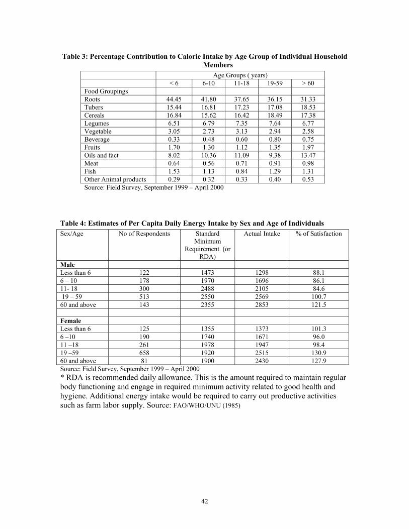
42

Table 3: Percentage Contribution to Calorie Intake by Age Group of Individual Household Members

Age Groups ( years) < 6 6-10 11-18 19-59 > 60 Food Groupings Roots 44.45 41.80 37.65 36.15 31.33 Tubers 15.44 16.81 17.23 17.08 18.53 Cereals 16.84 15.62 16.42 18.49 17.38 Legumes 6.51 6.79 7.35 7.64 6.77 Vegetable 3.05 2.73 3.13 2.94 2.58 Beverage 0.33 0.48 0.60 0.80 0.75 Fruits 1.70 1.30 1.12 1.35 1.97 Oils and fact 8.02 10.36 11.09 9.38 13.47 Meat 0.64 0.56 0.71 0.91 0.98 Fish 1.53 1.13 0.84 1.29 1.31 Other Animal products 0.29 0.32 0.33 0.40 0.53 Source: Field Survey, September 1999 – April 2000

Table 4: Estimates of Per Capita Daily Energy Intake by Sex and Age of Individuals Sex/Age No of Respondents Standard

Minimum Requirement (or

RDA)

Actual Intake % of Satisfaction

Male Less than 6 122 1473 1298 88.1 6 – 10 178 1970 1696 86.1 11- 18 300 2488 2105 84.6 19 – 59 513 2550 2569 100.7 60 and above 143 2355 2853 121.5 Female Less than 6 125 1355 1373 101.3 6 –10 190 1740 1671 96.0 11 –18 261 1978 1947 98.4 19 –59 658 1920 2515 130.9 60 and above 81 1900 2430 127.9 Source: Field Survey, September 1999 – April 2000 * RDA is recommended daily allowance. This is the amount required to maintain regular body functioning and engage in required minimum activity related to good health and hygiene. Additional energy intake would be required to carry out productive activities such as farm labor supply. Source: FAO/WHO/UNU (1985)

43

Table 5: Per Capita Calorie Intake by Education and Occupation of Household Head

A: Per Capita Calorie Intake by Age of Individual and Education level of Household Head

No of Respondents

Minimum Calorie Requirement per

Day (Kilocalories)

Actual Intake (Kilocalories)

% Satisfaction of

Minimum

Below Secondary School Less than 6 140 1415.25 1385 97.86 6 – 10 255 1855 1732 93.40 11 – 18 410 2232.5 2019 90.44 19 – 59 818 2232 2568 114.90 60 and above 204 2070 2710 130.92 Secondary School & Above Less than 6 107 1415.25 1275 89.88 6 – 10 143 1855 1607 86.63 11 – 18 151 2232.5 2066 92.54 19 – 59 353 2235 2471 110.56 60 and above 20 2070 2603 125.75 B: Per Capita Calorie Intake by Age of Individual and Occupation of Household Head Food Sector Less than 6 118 1415.25 1423 100.55 6 –10 187 1855 1785 96.23 11 – 18 358 2232.5 2106 94.29 19 – 59 670 2235 2619 117.18 60 and above 168 2070 2721 131.45 Non- food sector Less than 6 128 1415.25 1261 89.10 6 –10 180 1855 1583 85.34 11 – 18 200 2232.5 1900 85.11 19 – 59 492 2235 2438 109.08 60 and above 56 2070 2636 127.34 Source: Field Survey, September 1999 – April 2000

44

Table 6: Description of Model Variables Variable Mean Std Deviation

Left hand side endogenous variables Natural log of Individual daily calorie intake 7.591 0.486 Natural log of Individual daily food expenditure 3.998 0.509 Natural log calorie price 1.012 0.279 Cash purchase share in total food expenditure (ratio) 0.574 0.327 Right hand side endogenous variables Natural log of per capita consumption expenditure 7.291 0.901 Women’s share of household income (ratio) 0.305 0.272 Right hand side controls Age 26.7 19.4 Number of wives 1.30 0.810 Number of female aged in household (60+) 0.170 0.450 Number of male aged in household 0.350 0.550 Number of female adults in household (19-59) 1.59 1.000 Number of male adults in households (19-59) 1.26 1.23 Number of female adolescents in household ( 11-18 years ) 0.690 1.000 Number of male adolescents in household ( 11-18 years ) 0.810 0.920 Major occupation of household head ( Non-Farming =1, Farming =0) 0.587 0.492 Major occupation of senior wife ( Non-Farming =1, Farming =0) 0.703 0.457 Yam price ( N/kilogram) 13.0 7.46 Cassava flour price( N/kilogram) 27.7 20.0 Yam flour price ( N/kilogram) 60.3 34.7 Cowpeas price ( N/kilogram) 48.5 9.30 Rice price ( N/kilogram) 56.1 4.25 Maize price ( N/kilogram) 30.1 8.71 Gari price ( N/kilogram) 14.6 3.97 Palm oil price ( N/kilogram) 102.1 17.1 Beef price ( N/kilogram) 249.3 138.1 Fish price ( N/kilogram) 152.6 115.8 Exclusion restrictions used to identify 2SLS Total Years of schooling of husband and wife 9.40 9.60 Ratio of senior wife’s to husband’s education 0.420 0.580 Value of total assets of households in Naira value ($1= 80 Naira) 810506.0 1941756.0 Women’s share of total business asset (ratio) 0.304 0.341 Other interesting variables not in final model Individual daily calorie intake 2204.0 969.0 Unit cost of calorie intake ( Naira/100 kilocalories) 2.857 0.769 Per capita consumption expenditure (N/month) 2135.0 1894.0 Household size ( no of persons) 7.11 3.26 Value of farm assets of households (Naira) 124533.0 269392.0 Women’s share of farm size (ratio) 0.144 0.294 Years of education of household head 5.08 5.43 Years of education of senior wife 4.31 5.02 Women’s share of household farmland value (ratio) 0.0703 0.180 Women’s share of food expenditure (ratio ) 0.321 0.301 Women’s food share in total women expenditure (ratio) 0.320 0.246 Women’s share of home consumed farm produce. (ratio) 17.0 30.5 Women’s share of value of crops on farm. (ratio) 11.1 26.8

Source: field survey, August 1999-April 2000

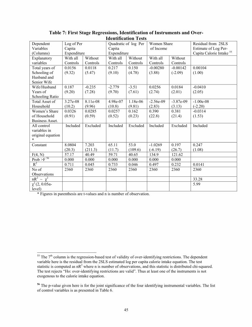
45

Table 7: First Stage Regressions, Identification of Instruments and Over-Identification Tests

Dependent Variables (Columns)

Log of Per Capita Expenditure

Quadratic of log Per Capita Expenditure

Women Share of Income

Residual from 2SLS Estimate of Log Per- Capita Calorie Intake 55

Explanatory variables

With all Controls

Without Controls

With all Controls

Without Controls

With all Controls

Without Controls

Total years of Schooling of Husband and Senior Wife

0.0156 (9.32)

0.0118 (5.47)

0.217 (9.10)

0.150 (4.78)

-0.00280 (3.88)

-0.00142 (-2.09)

0.00104 (1.00)

Wife/Husband Years of Schooling Ratio

0.187 (9.20)

-0.235 (7.28)

-2.779 (9.70)

-3.51 (7.61)

0.0256 (2.74)

0.0184 (2.01)

-0.0410 (2.05)

Total Asset of Household

3.27e-08 (10.2)

8.11e-08 (9.96)

4.98e-07 (10.8)

1.18e-06 (9.81)

-2.56e-09 (2.83)

-3.87e-09 (3.13)

-1.00e-08 (-2.20)

Women’s Share of Household Business Asset.

0.0326 (0.91)

0.0285 (0.59)

0.0257 (0.52)

0.162 (0.23)

0.390 (22.8)

0.381 (21.4)

-0.0314 (1.53)

All control variables in original equation *

Included Excluded Included Excluded Included Excluded Included

Constant

8.0804 (20.3)

7.203 (211.3)

65.11 (11.7)

53.0 (109.6)

-1.0269 (-6.19)

0.197 (26.7)

0.247 (1.08)

F(4, N) 57.17 40.49 59.71 40.65 134.9 121.62 Prob >F 56 0.000 0.000 0.000 0.000 0.000 0.000 R2 0.711 0.045 0.733 0.046 0.497 0.232 0.0141 No of Observations

2360 2360 2360 2360 2360 2360 2360

nR2 ~ χ2 33.28 χ2 (2, 0.05α-level)

5.99

* Figures in parenthesis are t-values and n is number of observation.

55 The 7th column is the regression-based test of validity of over-identifying restrictions. The dependent variable here is the residual from the 2SLS estimated log per capita calorie intake equation. The test statistic is computed as nR2 where n is number of observations, and this statistic is distributed chi-squared. The test rejects “Ho: over-identifying restrictions are valid”. Thus at least one of the instruments is not exogenous to the calorie intake equation. 56 The p-value given here is for the joint significance of the four identifying instrumental variables. The list of control variables is as presented in Table 6.

46

Table 8: Results of Test of Endogeniety of Per-Capita Expenditure and Women’s Share of Income

Dependent Variables57 Residuals from OLS Estimated Log Per-Capita Calorie Intake Equation

With log-linear Per-Capita Expenditure

With Quadratic Per-Capita Expenditure

Explanatory Variables Residual from first stage regression for log per capita expenditure

0.00455 (0.39)

-0.00296 (0.03)

Residual from first stage regression of per capita expenditure squared

0.000446 (0.0.06)

Residual from first stage regression of women’s share of household income

0.242 (0.81)

0.0297 (1.00)

Constant -0.000421 (0.07)

-0.000286 (0.05)

Prob > F 58 0.665 0.782 * * Figures in parenthesis are t-values.

57 The dependent variables are residuals from the OLS estimate of the full structural equation as presented in the second and fourth column of Table 9. 58 The p-values of 0.665 and 0.782 imply an inability to reject the null hypothesis that per capita expenditure and women’s share of income are exogenous in this model.

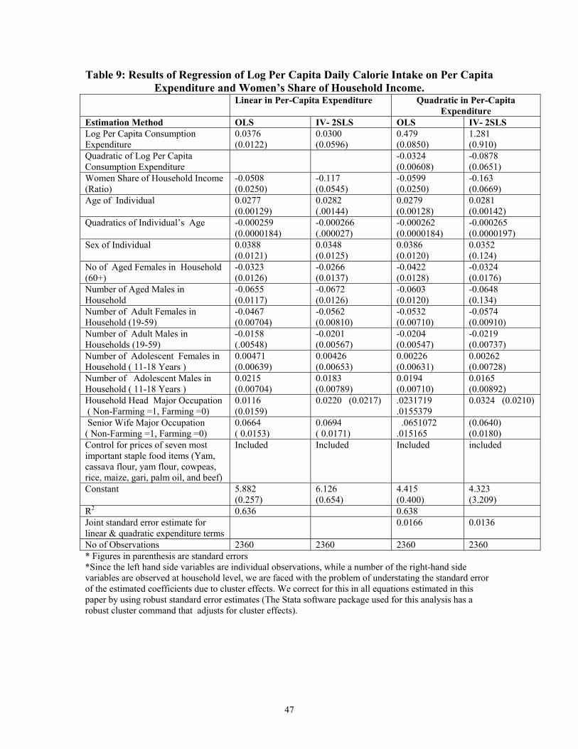
47

Table 9: Results of Regression of Log Per Capita Daily Calorie Intake on Per Capita Expenditure and Women’s Share of Household Income.

Linear in Per-Capita Expenditure Quadratic in Per-Capita Expenditure

Estimation Method OLS IV- 2SLS OLS IV- 2SLS Log Per Capita Consumption Expenditure

0.0376 (0.0122)

0.0300 (0.0596)

0.479 (0.0850)

1.281 (0.910)

Quadratic of Log Per Capita Consumption Expenditure

-0.0324 (0.00608)

-0.0878 (0.0651)

Women Share of Household Income (Ratio)

-0.0508 (0.0250)

-0.117 (0.0545)

-0.0599 (0.0250)

-0.163 (0.0669)

Age of Individual

0.0277 (0.00129)

0.0282 (.00144)

0.0279 (0.00128)

0.0281 (0.00142)

Quadratics of Individual’s Age

-0.000259 (0.0000184)

-0.000266 (.000027)

-0.000262 (0.0000184)

-0.000265 (0.0000197)

Sex of Individual

0.0388 (0.0121)

0.0348 (0.0125)

0.0386 (0.0120)

0.0352 (0.124)

No of Aged Females in Household (60+)

-0.0323 (0.0126)

-0.0266 (0.0137)

-0.0422 (0.0128)

-0.0324 (0.0176)

Number of Aged Males in Household

-0.0655 (0.0117)

-0.0672 (0.0126)

-0.0603 (0.0120)

-0.0648 (0.134)

Number of Adult Females in Household (19-59)

-0.0467 (0.00704)

-0.0562 (0.00810)

-0.0532 (0.00710)

-0.0574 (0.00910)

Number of Adult Males in Households (19-59)

-0.0158 (.00548)

-0.0201 (0.00567)

-0.0204 (0.00547)

-0.0219 (0.00737)

Number of Adolescent Females in Household ( 11-18 Years )

0.00471 (0.00639)

0.00426 (0.00653)

0.00226 (0.00631)

0.00262 (0.00728)

Number of Adolescent Males in Household ( 11-18 Years )

0.0215 (0.00704)

0.0183 (0.00789)

0.0194 (0.00710)

0.0165 (0.00892)

Household Head Major Occupation ( Non-Farming =1, Farming =0)

0.0116 (0.0159)

0.0220 (0.0217) .0231719 .0155379

0.0324 (0.0210)

Senior Wife Major Occupation ( Non-Farming =1, Farming =0)

0.0664 ( 0.0153)

0.0694 ( 0.0171)

.0651072 .015165

(0.0640) (0.0180)

Control for prices of seven most important staple food items (Yam, cassava flour, yam flour, cowpeas, rice, maize, gari, palm oil, and beef)

Included Included Included included

Constant

5.882 (0.257)

6.126 (0.654)

4.415 (0.400)

4.323 (3.209)

R2 0.636 0.638 Joint standard error estimate for linear & quadratic expenditure terms

0.0166 0.0136

No of Observations 2360 2360 2360 2360 * Figures in parenthesis are standard errors *Since the left hand side variables are individual observations, while a number of the right-hand side variables are observed at household level, we are faced with the problem of understating the standard error of the estimated coefficients due to cluster effects. We correct for this in all equations estimated in this paper by using robust standard error estimates (The Stata software package used for this analysis has a robust cluster command that adjusts for cluster effects).

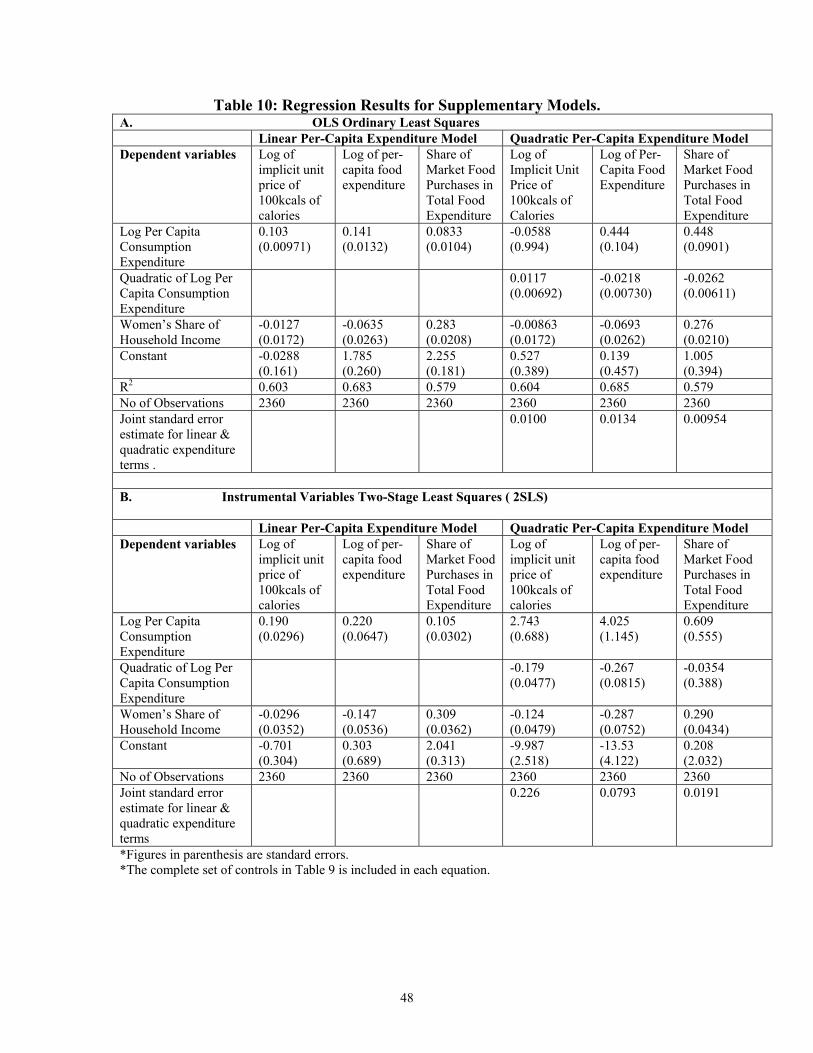
48

Table 10: Regression Results for Supplementary Models. A. OLS Ordinary Least Squares Linear Per-Capita Expenditure Model Quadratic Per-Capita Expenditure Model Dependent variables Log of

implicit unit price of 100kcals of calories

Log of per-capita food expenditure

Share of Market Food Purchases in Total Food Expenditure

Log of Implicit Unit Price of 100kcals of Calories

Log of Per-Capita Food Expenditure

Share of Market Food Purchases in Total Food Expenditure

Log Per Capita Consumption Expenditure

0.103 (0.00971)

0.141 (0.0132)

0.0833 (0.0104)

-0.0588 (0.994)

0.444 (0.104)

0.448 (0.0901)

Quadratic of Log Per Capita Consumption Expenditure

0.0117 (0.00692)

-0.0218 (0.00730)

-0.0262 (0.00611)

Women’s Share of Household Income

-0.0127 (0.0172)

-0.0635 (0.0263)

0.283 (0.0208)

-0.00863 (0.0172)

-0.0693 (0.0262)

0.276 (0.0210)

Constant

-0.0288 (0.161)

1.785 (0.260)

2.255 (0.181)

0.527 (0.389)

0.139 (0.457)

1.005 (0.394)

R2 0.603 0.683 0.579 0.604 0.685 0.579 No of Observations 2360 2360 2360 2360 2360 2360 Joint standard error estimate for linear & quadratic expenditure terms .

0.0100 0.0134 0.00954

B. Instrumental Variables Two-Stage Least Squares ( 2SLS)

Linear Per-Capita Expenditure Model Quadratic Per-Capita Expenditure Model Dependent variables Log of

implicit unit price of 100kcals of calories

Log of per-capita food expenditure

Share of Market Food Purchases in Total Food Expenditure

Log of implicit unit price of 100kcals of calories

Log of per-capita food expenditure

Share of Market Food Purchases in Total Food Expenditure

Log Per Capita Consumption Expenditure

0.190 (0.0296)

0.220 (0.0647)

0.105 (0.0302)

2.743 (0.688)

4.025 (1.145)

0.609 (0.555)

Quadratic of Log Per Capita Consumption Expenditure

-0.179 (0.0477)

-0.267 (0.0815)

-0.0354 (0.388)

Women’s Share of Household Income

-0.0296 (0.0352)

-0.147 (0.0536)

0.309 (0.0362)

-0.124 (0.0479)

-0.287 (0.0752)

0.290 (0.0434)

Constant

-0.701 (0.304)

0.303 (0.689)

2.041 (0.313)

-9.987 (2.518)

-13.53 (4.122)

0.208 (2.032)

No of Observations 2360 2360 2360 2360 2360 2360 Joint standard error estimate for linear & quadratic expenditure terms

0.226 0.0793 0.0191

*Figures in parenthesis are standard errors. *The complete set of controls in Table 9 is included in each equation.

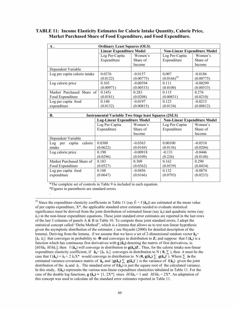
49

TABLE 11: Income Elasticity Estimates for Calorie Intake Quantity, Calorie Price, Market Purchased Share of Food Expenditure, and Food Expenditure.

A . Ordinary Least Squares (OLS)

Linear Expenditure Model Non-Linear Expenditure Model Log Per-Capita Expenditure

Women’s Share of Income

Log Per-Capita Expenditure

Women’s Share of Income

Dependent Variable Log per capita calorie intake 0.0376

(0.0122) -0.0157 (0.00775)

0.007 (0.0166)59

-0.0186 (0.00775)

Log calorie price 0.103 (0.00971)

-0.00394 (0.00533)

0.111 (0.0100)

-0.00299 (0.00533)

Market Purchased Share of Food Expenditure

0.145) (0.0181)

0.283 (0.0208)

0.115 (0.00831)

0.276 (0.0210)

Log per capita food expenditure

0.140 (0.0132)

-0.0197 (0.00815)

0.123 (0.0134)

-0.0215 (0.00812)

B. Instrumental Variable Two Stage least Squares (2SLS)

Log-Linear Expenditure Model Non-Linear Expenditure Model Log Per-Capita Expenditure

Women’s Share of Income

Log Per-Capita Expenditure

Women’s Share of Income

Dependent Variable Log per capita calorie intake

0.0300 (0.0622)

-0.0363 (0.0169)

0.00100 (0.0136)

-0.0510 (0.0204)

Log calorie price 0.190 (0.0296)

-0.00918 (0.0109)

-0.131 (0.226)

-0.0446 (0.0148)

Market Purchased Share of Food Expenditure

0.183 (0.0527)

0.309 (0.0362)

0.162 (0.0539)

0.290 (0.0434)

Log per capita food expenditure

0.188 (0.0647)

-0.0456 (0.0166)

0.132 (0.0793)

-0.0874 (0.0233)

*The complete set of controls in Table 9 is included in each equation. *Figures in parenthesis are standard errors. .

59 Since the expenditure elasticity coefficients in Table 11 (say Ê = f (ân)) are estimated at the mean value of per capita expenditure, X*, the applicable standard error estimate needed to evaluate statistical significance must be derived from the joint distribution of estimated linear (say â0) and quadratic terms (say â1) in the non-linear expenditure equations. These joint standard error estimates are reported in the last rows of the last 3 columns of panels A & B in Table 10. To compute these joint standard errors, I adopt the statistical concept called “Delta Method”, which is a lemma that allows us to test non-linear hypothesis given the asymptotic distribution of the estimator. ( see Hayashi (2000) for detailed description of the lemma). Deriving from the lemma, if we assume that we have a set of 2-dimensional random vector ân= [â0 â1] that converges in probability to Φ and converges in distribution to Z; and suppose that f (ân) is a function which has continuous first derivatives with g (ân) denoting the matrix of first derivatives, ie. [δf/δâ0 δf/δâ1]; then f (ân) will converge in distribution to g(ân)Z . Thus, for the calorie intake non-linear expenditure elasticity coefficient, if ân= [â0 â1] converges in distribution to N ( 0, ∑ ), then it must be the case that f (ân) = â0 + 2 â1X* would converge in distribution to N (0, g(ân) ∑ g(ân)' ). Where ∑ is the estimated variance-covariance matrix of ân. and {g(ân) ∑ g(ân)' } is the variance of f(ân) given the joint distribution of the â0 and â1 . The standard error of f(ân) is just the square root of the calculated variance. In this study, f(ân) represents the various non-linear expenditure elasticities tabulated in Table 11. For the case of the double log functions, g (ân) = [1, 2X*] since δf/δâ0 = 1 and δf/δâ1 = 2X*. An adaptation of this concept was used to calculate all the standard error estimates reported in Table 11.