HAL Id: hal-01629342https://hal.archives-ouvertes.fr/hal-01629342

Submitted on 29 Jan 2018

HAL is a multi-disciplinary open accessarchive for the deposit and dissemination of sci-entific research documents, whether they are pub-lished or not. The documents may come fromteaching and research institutions in France orabroad, or from public or private research centers.

L’archive ouverte pluridisciplinaire HAL, estdestinée au dépôt et à la diffusion de documentsscientifiques de niveau recherche, publiés ou non,émanant des établissements d’enseignement et derecherche français ou étrangers, des laboratoirespublics ou privés.

Interval observer for LPV systems: Application tovehicle lateral dynamics

Sara Ifqir, Naima Ait Oufroukh, Dalil Ichalal, Saïd Mammar

To cite this version:Sara Ifqir, Naima Ait Oufroukh, Dalil Ichalal, Saïd Mammar. Interval observer for LPV systems:Application to vehicle lateral dynamics. 20th World Congress of the International Federation ofAutomatic Control, Jul 2017, Toulouse, France. pp.7572–7577, �10.1016/j.ifacol.2017.08.995�. �hal-01629342�

Interval observer for LPV systems:Application to vehicle lateral dynamics

S. Ifqir ∗ N. Ait Oufroukh ∗ D. Ichalal ∗ S. Mammar ∗

∗ Laboratory of Computing, Integrative Biology and Complex Systems,University of Evry Val dEssonne, Evry 91000, France, (e-mail:{

sara.ifqir, naima.aitoufroukh, dalil.ichalal, said.mammar}@ibisc.univ-evry.fr ).

Abstract: This paper presents a new method for guaranteed and robust estimation of sideslipangle and lateral tire forces with consideration of cornering stiffness variations resulting fromchanges in tire/road and driving conditions. An interval LPV observer with both measurableand unmeasurable time-varying parameters is proposed. The longitudinal velocity is treated asthe online measured time-varying parameter and the cornering stiffness at front and rear tiresare assumed to be unknown but bounded with a priori known bounds. The obtained results areno more punctual values but a set of acceptable values. The simulation is based on experimentaldata in order to prove the effectiveness of the proposed observers.

Keywords: Interval observer, uncertain systems, robustness, positive systems, eigenvalueassignment, state estimation, vehicle lateral dynamics.

1. INTRODUCTION

Accurate knowledge of state variables such as sideslipangle and tire forces is essential to improve the safety,handling, performance and comfort of vehicles. However,the complexity of the technical implementation and costprohibitive for the installation of sensors to measure theseimportant data make their integration into standard ve-hicles an unfeasible solution. Therefore, these variablesmust be estimated using observers and measurements fromstandard sensors such as gyro, accelerometer, etc.

In the literature, several studies have addressed the de-sign of classic observers to estimate the vehicle lateraldynamic states using different approaches. For example,Luenberger observer, Kalman Filter (Venhovens and Naab(1999)), Extended Kalman filter (Satria and Best (2005)),Unknown input proportional-integral observer (Mammaret al. (2006)) and sliding mode observer (Stephant et al.(2007)). Most of these studies have been based on theassumption that the cornering stiffness parameters areconstant. This assumption is verified only when the vehicleis operating in the linear region of lateral forces (Fig. 2)and the road conditions are nominal. However, when theroad friction changes, the nonlinear region is generallyreached. Consequently, the vehicle approaches to its op-erational limit conditions and its response to the driver’sinputs becomes less responsive making these parameters asan obstacle in developing a high performance estimator.

In (M’sirdi et al. (2005)), a sliding mode observer (SMO)has been used to identify the tire/road parameters. It isone of the popular robust approaches, in fact, the slidingsurface ensures the robustness of the parameter variations.However, the main disadvantage of the sliding mode tech-nique is the undesirable chattering phenomenon (Utkin

?

et al. (2009)). Another popular approach is presentedin (Hiraoka et al. (2004)) using adaptive observer. Thismethod suffers from a significant disadvantage that is theexistence of solution satisfying the sufficient conditionsis not always guaranteed. Furthermore, an accurate es-timate of the parameters requires that the system inputsto satisfy the conditions of persistent excitation. In (Ray(1997)), a extended Kalman-Bucy filtering (EKBF) is usedto estimate lateral forces, which are treated as randomvariables. This method allows to achieve precise parameterestimates, but requires accurate knowledge of the modeland noise statistics.

In the last decades, the development of the intervalobserver (Gouze et al. (2000), Rapaport and Harmand(2002)) represent an alternative technique for robust es-timation in the presence of parameter uncertainties, un-known inputs or measurement disturbances. It becomes, apopular successful robust approach especially in biotech-nological domain (Rapaport and Dochain (2005), Meslemet al. (2008)). Note that, interval observers can be definedas a pair of estimators based on Luenberger structurewhich provide a guaranteed bounds covering all admis-sible trajectories of system, using a priori known boundson uncertain parameters and/or exogenous disturbances.The synthesis of these observers often uses an additionalassumptions to prove the stability of the estimated bounds,the monotony and cooperativity (Smith (2008)). Theseproperties keep the partial order between lower and uppertrajectories.

Several interval observers are proposed in the literature.For instance, in Rami et al. (2008), Bolajraf et al. (2010)and Rami et al. (2013), interval observers for linear uncer-tain systems are presented. The necessary and sufficientconditions have been formulated in terms of linear pro-gramming. The case of the LPV and nonlinear systems

are treated in Raıssi et al. (2010), Efimov et al. (2012)and Efimov et al. (2013) using the Lyapunov theory andlinear matrix inequalities (LMIs). In this paper, an intervalobserver for LPV systems which contain unmeasured andmeasured uncertain parameters is proposed. The observeris based on a robust pole assignment depending on theparameter variation.

The present paper is organized as follows. Some prelimi-naries are given in section 2. In section 3, we present theuncertain LPV system of the vehicle lateral dynamics. Thesection 4 is devoted to the main result. The Experimentalresults are provided in section 5. A conclusion is drawn insection 6 and end the technical note.

2. PRELIMINARIES

The objective of this section is to provide some notationsand basic definitions that are used throughout the paper.

• A vector with null components is denoted by 0.• The absolute value of x is denoted by |x|.• The norm L∞ of x is denoted by ‖x‖.• The left and right endpoints of an interval [x] (resp.

a matrix M) are denoted respectively by x− and x+

(resp. M− and M+) such as [x] = [x−, x+] (resp.[M ] = [M−,M+]).

• All the inequalities must be interpreted element wise.• Let a vector x ∈ Rn or a matrix A ∈ Rn×n, one

denotes x = max{0, x}, x = x− x or A = max{0, A},A = A−A.• The eigenvalues of a matrix A are denoted λ.• A real matrix A is called Hurwitz if all its eigenvalues

have strictly negative real part (Re(λ < 0) ).• A real matrix A is called Metzler if all its elements

outside the main diagonal are positive (aij ≥ 0, ∀i 6=j).• A continuous-time linear system is cooperative if its

state matrix A is a Metzler matrix.

Lemma 1 (Gouze et al. (2000)) For a Metzler matrix A,the cooperative system:

x(t) = Ax(t) + d(t)

with x ∈ Rn and d : R → Rn+ is said to be positive ifx(0) ≥ 0 then x(t) ≥ 0, ∀t ≥ 0.Lemma 2 (Efimov et al. (2012)) Let x ∈ [x−, x+] be avariable vector, then for a variable matrix ∆A ∈ Rn×nsuch as ∆A− ≤ ∆A ≤ ∆A+ for some ∆A−, ∆A+ ∈ Rn×n,then

∆A+x+ −∆A+x− −∆A−x+ + ∆A

−x− ≤ ∆Ax ≤

∆A+x+ −∆A+x− −∆A

−x+ + ∆A−x−

(1)

3. VEHICLE LATERAL MODEL

Vehicle lateral dynamics could be modeled by a bicyclemodel which a two degree of freedom (2-DOF) vehiclemodel with sideslip angle and yaw rate as the states.The dynamics equations can be represented by (Rajamani(2011)): {

mvx(β + r) = Fyf + FyrIz r = lfFyf − lrFyr

(2)

where m, Iz, lr, lf denote respectively the mass of thevehicle, the yaw moment and the distances from the rear

Fig. 1. Bicycle Model.

and the front axle to the center of gravity. vx is a time-varying longitudinal velocity, β is the sideslip angle of thevehicle and r is the yaw rate. Fyr and Fyf are the lateralrear and front forces respectively.

The nonlinear forces Fyf and Fyr are usually functionsof the wheel sideslip angle and wheel longitudinal slip(Dugoff et al. (1970), Pacejka and Bakker (1991), Burck-hardt (1993), Kiencke and Nielsen (2000)). Using Pacejka’smagic formula (Pacejka and Bakker (1991)), the lateralforces are given by:

Fyi = Disin(Citan−1(Bi(1− Ei)αi + Eitan

−1(Biαi)))(3)

where i = {r, f} denotes rear and front of the vehicle.Di, Ci, Bi and Ei are the characteristic constants of thetires. αf and αr are respectively the front and rear sideslipangles of the tires expressed by (Cheng et al. (2011)):

αf = δf − β − tan−1(lf

vxrcos(β))

αr = −β + tan−1(lf

vxrcos(β))

(4)

For small variations of the sideslip angle (≤ 8◦), (4) maybe simplified as follows:

αf = δf − β −lfvxr

αr = −β +lrvxr

(5)

Fyf and Fyr are nonlinear forces but in this work the forcesare considered linear with respect to the sideslip angles ofthe tires (linear approximation of (3)):{

Fyf = cfαfFyr = crαr

(6)

cf and cr denote respectively the cornering stiffness offront and rear tires and they correspond to the slope atthe origin (Fig. 2). These parameters are closely related toroad friction. If road friction changes or if the nonlinear tireregion is reached, cornering stiffness varies. Consequently,we consider in this study that the cornering stiffness in(6) are expressed as a linear part (denoted ci0) and anuncertainty term (denoted ∆ci) assumed to be unknownbut bounded with a priori known bounds (Fig. 2):{

Fyf = (cf0 + ∆cf )αfFyr = (cr0 + ∆cr)αr

(7)

Gathering equations (2), (5) and (6) leads to the followingmodel:

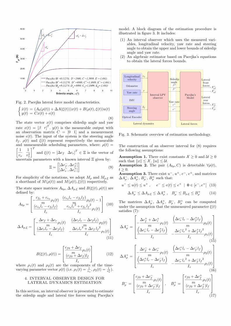
Fig. 2. Pacejka lateral force model characteristics.{x(t) = (A0(ρ(t)) + ∆A(ξ(t)))x(t) +B(ρ(t), ξ(t))u(t)y(t) = Cx(t) + e(t)

(8)The state vector x(t) comprises slideslip angle and yaw

rate x(t) = [β r]T

. y(t) is the measurable output withan observation matrix C = [0 1] and a measurementnoise e(t). The input of the system is the steering angleδf . ρ(t) and ξ(t) represent respectively the measurableand unmeasurable scheduling parameters, where: ρ(t) =[

1

vx

1

v2x

]Tand ξ(t) = [∆cf ∆cr]

T ∈ Ξ is the vector of

uncertain parameters with a known interval Ξ given by:

Ξ =

[[∆c−f ,∆c

+f ]

[∆c−r ,∆c+r ]

](9)

For simplicity of the notations, we adopt Mρ and Mρ,ξ asa shorthand of M(ρ(t)) and M(ρ(t), ξ(t)) respectively.

The state space matrices A0ρ, ∆Aρ,ξ and B(ξ(t), ρ(t)) aredefined by:

A0ρ =

−cf0 + cr0m

ρ1(t)(cr0 lr − cf0 lf )

mρ2(t)− 1

(cr0 lr − cf0 lf )

Iz−cr0 lr

2 + cf0 lf2

Izρ1(t)

(10)

∆Aρ,ξ =

−∆cf + ∆crm

ρ1(t)(∆crlr −∆cf lf )

mρ2(t)

(∆crlr −∆cf lf )

Iz−∆crlr

2 + ∆cf lf2

Izρ1(t)

(11)

B(ξ(t), ρ(t)) =

cf0 + ∆cfm

ρ1(t)

(cf0 + ∆cf )lfIz

(12)

where ρ1(t) and ρ2(t) are the components of the time-varying parameter vector ρ(t) (i.e. ρ1(t) = 1

vx, ρ2(t) = 1

v2x).

4. INTERVAL OBSERVER DESIGN FORLATERAL DYNAMICS ESTIMATION

In this section, an interval observer is presented to estimatethe sideslip angle and lateral tire forces using Pacejka’s

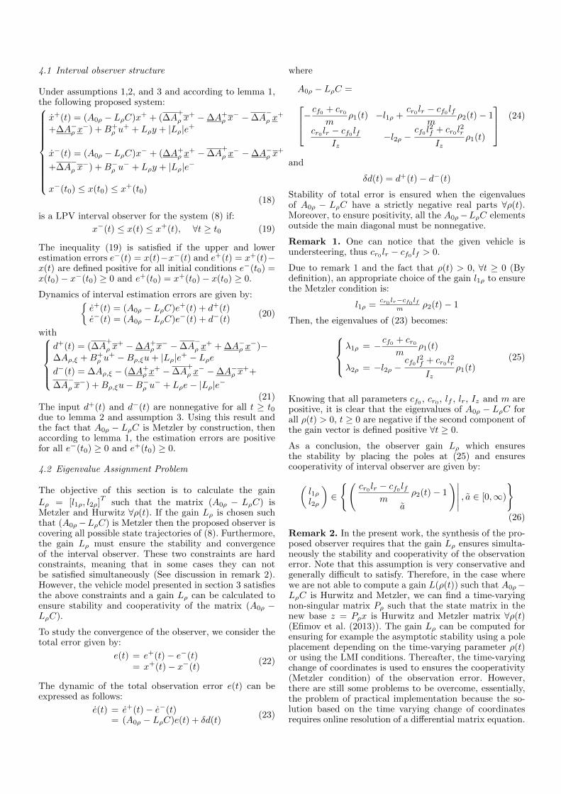
model. A block diagram of the estimation procedure isillustrated in figure 3. It includes:

(1) An interval observer which uses the measured vari-ables, longitudinal velocity, yaw rate and steeringangle to obtain the upper and lower bounds of sideslipangle and yaw rate.

(2) An algebraic estimator based on Pacejka’s equationsto obtain the lateral forces bounds.

Interval LPVobserver

Longitudinalvelocity

Yaw rate

Steeringangle

Pacejka’sModel

vx

r

δf

Odometer

IMU

Optical Encoder

Lateral dynamics

Sideslipangleβ+

β−

Yaw rater+

r−

Lateral forces

Lateralfrontforces

F+yf

F−yf

Lateralrearforces

F+yr

F−yr

Fig. 3. Schematic overview of estimation methodology.

The construction of an observer interval for (8) requiresthe following assumptions:

Assumption 1. There exist constants X ≥ 0 and U ≥ 0such that ‖x‖ ≤ X , ‖u‖ ≤ U .Assumption 2. The pair (A0ρ, C) is detectable ∀ρ(t),t ≥ 0.Assumption 3. There exist u−, u+, e−, e+, and matrices∆A−ρ , ∆A+

ρ , B−ρ , B+ρ such that:

u− ≤ u(t) ≤ u+ , e− ≤ e(t) ≤ e+ | 0 ∈ [e−, e+] (13)

∆A−ρ ≤ ∆Aρ,ξ ≤ ∆A+ρ , B−ρ ≤ Bρ,ξ ≤ B+

ρ (14)

The matrices ∆A−ρ , ∆A+ρ , B−ρ , B+

ρ can be computedunder the assumption that the unmeasured parameter ξ(t)satisfies (7):

∆A−ρ =

−

∆c+f + ∆c+r

mρ1(t)

(∆c−r lr −∆c+f lf

)m

ρ2(t)(∆c−r lr −∆c+f lf

)Iz

−∆c+r lr

2 + ∆c+f lf2

Izρ1(t)

(15)

∆A+ρ =

−

∆c−f + ∆c−r

mρ1(t)

(∆c+r lr −∆c−f lf

)m

ρ2(t)(∆c+r lr −∆c−f lf

)Iz

−∆c−r lr

2 + ∆c−f lf2

Izρ1(t)

(16)

B−ρ =

cf0 + ∆c−f

mρ1(t)

(cf0 + ∆c−f )lf

Iz

, B+ρ =

cf0 + ∆c+f

mρ1(t)

(cf0 + ∆c+f )lf

Iz

(17)

4.1 Interval observer structure

Under assumptions 1,2, and 3 and according to lemma 1,the following proposed system:

x+(t) = (A0ρ − LρC)x+ + (∆A+

ρ x+ −∆A+

ρ x− −∆A

−ρ x

+

+∆A−ρ x−) +B+

ρ u+ + Lρy + |Lρ|e+

x−(t) = (A0ρ − LρC)x− + (∆A+ρ x

+ −∆A+

ρ x− −∆A−ρ x

+

+∆A−ρ x−) +B−ρ u

− + Lρy + |Lρ|e−

x−(t0) ≤ x(t0) ≤ x+(t0)(18)

is a LPV interval observer for the system (8) if:

x−(t) ≤ x(t) ≤ x+(t), ∀t ≥ t0 (19)

The inequality (19) is satisfied if the upper and lowerestimation errors e−(t) = x(t)−x−(t) and e+(t) = x+(t)−x(t) are defined positive for all initial conditions e−(t0) =x(t0)− x−(t0) ≥ 0 and e+(t0) = x+(t0)− x(t0) ≥ 0.

Dynamics of interval estimation errors are given by:{e+(t) = (A0ρ − LρC)e+(t) + d+(t)e−(t) = (A0ρ − LρC)e−(t) + d−(t)

(20)

withd+(t) = (∆A

+

ρ x+ −∆A+

ρ x− −∆A

−ρ x

+ + ∆A−ρ x−)−

∆Aρ,ξ +B+ρ u

+ −Bρ,ξu+ |Lρ|e+ − Lρed−(t) = ∆Aρ,ξ − (∆A+

ρ x+ −∆A

+

ρ x− −∆A−ρ x

++

∆A−ρ x−) +Bρ,ξu−B−ρ u− + Lρe− |Lρ|e−

(21)The input d+(t) and d−(t) are nonnegative for all t ≥ t0due to lemma 2 and assumption 3. Using this result andthe fact that A0ρ − LρC is Metzler by construction, thenaccording to lemma 1, the estimation errors are positivefor all e−(t0) ≥ 0 and e+(t0) ≥ 0.

4.2 Eigenvalue Assignment Problem

The objective of this section is to calculate the gain

Lρ = [l1ρ, l2ρ]T

such that the matrix (A0ρ − LρC) isMetzler and Hurwitz ∀ρ(t). If the gain Lρ is chosen suchthat (A0ρ−LρC) is Metzler then the proposed observer iscovering all possible state trajectories of (8). Furthermore,the gain Lρ must ensure the stability and convergenceof the interval observer. These two constraints are hardconstraints, meaning that in some cases they can notbe satisfied simultaneously (See discussion in remark 2).However, the vehicle model presented in section 3 satisfiesthe above constraints and a gain Lρ can be calculated toensure stability and cooperativity of the matrix (A0ρ −LρC).

To study the convergence of the observer, we consider thetotal error given by:

e(t) = e+(t)− e−(t)= x+(t)− x−(t)

(22)

The dynamic of the total observation error e(t) can beexpressed as follows:

e(t) = e+(t)− e−(t)= (A0ρ − LρC)e(t) + δd(t)

(23)

where

A0ρ − LρC =−cf0 + cr0

mρ1(t) −l1ρ +

cr0 lr − cf0 lfm

ρ2(t)− 1

cr0 lr − cf0 lfIz

−l2ρ −cf0 l

2f + cr0 l

2r

Izρ1(t)

(24)

and

δd(t) = d+(t)− d−(t)

Stability of total error is ensured when the eigenvaluesof A0ρ − LρC have a strictly negative real parts ∀ρ(t).Moreover, to ensure positivity, all the A0ρ−LρC elementsoutside the main diagonal must be nonnegative.

Remark 1. One can notice that the given vehicle isundersteering, thus cr0 lr − cf0 lf > 0.

Due to remark 1 and the fact that ρ(t) > 0, ∀t ≥ 0 (Bydefinition), an appropriate choice of the gain l1ρ to ensurethe Metzler condition is:

l1ρ =cr0 lr−cf0 lf

m ρ2(t)− 1

Then, the eigenvalues of (23) becomes:λ1ρ = −cf0 + cr0

mρ1(t)

λ2ρ = −l2ρ −cf0 l

2f + cr0 l

2r

Izρ1(t)

(25)

Knowing that all parameters cf0 , cr0 , lf , lr, Iz and m arepositive, it is clear that the eigenvalues of A0ρ − LρC forall ρ(t) > 0, t ≥ 0 are negative if the second component ofthe gain vector is defined positive ∀t ≥ 0.

As a conclusion, the observer gain Lρ which ensuresthe stability by placing the poles at (25) and ensurescooperativity of interval observer are given by:(

l1ρl2ρ

)∈

{(cr0 lr − cf0 lf

mρ2(t)− 1

a

)∣∣∣∣∣ , a ∈ [0,∞)

}(26)

Remark 2. In the present work, the synthesis of the pro-posed observer requires that the gain Lρ ensures simulta-neously the stability and cooperativity of the observationerror. Note that this assumption is very conservative andgenerally difficult to satisfy. Therefore, in the case wherewe are not able to compute a gain L(ρ(t)) such that A0ρ−LρC is Hurwitz and Metzler, we can find a time-varyingnon-singular matrix Pρ such that the state matrix in thenew base z = Pρx is Hurwitz and Metzler matrix ∀ρ(t)(Efimov et al. (2013)). The gain Lρ can be computed forensuring for example the asymptotic stability using a poleplacement depending on the time-varying parameter ρ(t)or using the LMI conditions. Thereafter, the time-varyingchange of coordinates is used to ensures the cooperativity(Metzler condition) of the observation error. However,there are still some problems to be overcome, essentially,the problem of practical implementation because the so-lution based on the time varying change of coordinatesrequires online resolution of a differential matrix equation.

4.3 Algebraic estimation of tire forces bounds

The idea now is to estimate the lateral forces using thealgebraic formula of the linearized Pacejka’s model andthe bounds previously estimated, we can express the upperand lower bounds of lateral forces by:

F+yf = c+f α

+f

F−yf = c−f α−f

F+yr = c+r α

+r

F−yr = c−r α−r

(27)

The measured parameter ρ(t), the steering angle δf , theupper and lower bounds ψ+, ψ−, β+ and β− of yaw rateand sideslip angle are then used for compute the boundsof tire slip angles αf and αr, where:

α−f = δf − β+ − lfρ1(t)r+

α+f = δf − β− − lfρ1(t)r−

α−r = −β+ + lrρ1(t)r−

α+r = −β− + lrρ1(t)r+

(28)

5. EXPERIMENTAL RESULTS

The interval observers are now tested on a data setacquired using a prototype vehicle. The run was performedon at test track located in the city of Versailles-Satory(France). The track is 3.5Km length with various curveprofiles allowing vehicle dynamics excitation.

Several sensors are implemented on the vehicle: The yawrate r is measured using an inertial unit, the steering angleδf is measured by an absolute optical encoder while anodometer provides the vehicle longitudinal speed. Finally,a high precision Correvit sensor provide a measure of thesideslip angle. This measure is not used for observer design.It serves only for observer estimation evaluation. Thesteering angle and the vehicle longitudinal speed profilesare shown in figures 3 and 4. One can see that the speedshould be treated as a time-varying parameter.

In addition, on can see from these figures that the steeringangle at the tire level reaches 0.1 rad while the speedis about 14 m/s. The corresponding lateral accelerationis about 4.2 m/s2. The lateral forces reach thus thenonlinear zone. Finally, for our purpose, we assume thatthe cornering stiffness parameters are affected of 10%uncertainty in their value.

The results for the LPV interval observer (18) are shownin Fig. 6, 7, 8 and 9, the interval observer providesthe guaranteed bounds covering the trajectory of statevariables. The algebraically reconstructed lateral forcesfulfill the interval requirements. During the maneuver,both the front and the rear tire forces saturate. One cansee on figure 10 that the real front tire force is within theenvelope defined by the interval observer both in the linearand the nonlinear region.

The initial conditions are chosen different from that ofthe measurements. The convergence time is short and theintervals width are tight. In figure 11, the interval errorseβ = β+ − β− and er = r+ − r− are shown. We note thatthe interval width is related to the model (8) uncertainty.If the corning stiffness parameters are perfectly knownand the model does not contain uncertainties therefore

estimated bounds will converge asymptotically to the realstate.

Fig. 4. Steering angle.

Fig. 5. Longitudinal velocity.

Fig. 6. Interval estimation for sideslip angle.

Fig. 7. Interval estimation for yaw rate.

Fig. 8. Interval estimation for the front lateral tire force.

6. CONCLUSION

In this work, it has been shown how one can use in-terval observers for a robust estimation of sideslip angle

Fig. 9. Interval estimation for the rear lateral tire force.

Fig. 10. Interval observer of the real front tire force.

Fig. 11. Interval errors eβ and er.

and lateral tire forces form a two-wheeled vehicle modelsubject to interval uncertainties (cornering stiffness). Thelongitudinal velocity is treated as the online measurabletime-varying parameter, the proposed interval observeris time-varying in respect to ρ(t). The simulation resultsdemonstrate the validity of proposed approach.

REFERENCES

Bolajraf, M., Rami, M.A., and Tadeo, F. (2010). Robustinterval observer with uncertainties in the output. In18th Mediterranean Conference on Control and Automa-tion, MED’10.

Burckhardt, M. (1993). Fahrwerktechnik: radschlupf-regelsysteme. Vogel-Verlag.

Cheng, Q., Victorino, A.C., and Charara, A. (2011). Non-linear observer of sideslip angle using a particle filterestimation methodology. IFAC Proceedings Volumes,44(1), 6266–6271.

Dugoff, H., Fancher, P., and Segel, L. (1970). An analysisof tire traction properties and their influence on vehicledynamic performance. SAE Technical Paper 700377.

Efimov, D., Fridman, L., Raıssi, T., Zolghadri, A., andSeydou, R. (2012). Interval estimation for LPV systemsapplying high order sliding mode techniques. Automat-ica, 40, 2365–2371.

Efimov, D., Raıssi, T., Chebotarev, S., and Zolghadri, A.(2013). Interval state observer for nonlinear time varyingsystems. Automatica, 49(1), 200–205.

Gouze, J., Rapaport, A., and Hadj-Sadok, M. (2000).Interval observers for uncertain biological systems. Eco-logical Modelling, 133, 45–56.

Hiraoka, T., Kumamoto, H., and Nishihara, O. (2004).Sideslip angle estimation and active front steering sys-tem based on lateral acceleration data at centers ofpercussion with respect to front/rear wheels. JSAEreview, 25(1), 37–42.

Kiencke, U. and Nielsen, L. (2000). Automotive controlsystem. Springer.

Mammar, S., Glaser, S., and Netto, M. (2006). Vehi-cle lateral dynamics estimation using unknown inputproportional-integral observers. In 2006 American con-trol conference, 6–pp. IEEE.

Meslem, N., Ramdani, N., and Candau, Y. (2008). Intervalobservers for uncertain nonlinear systems. applicationto bioreactors. IFAC Proceedings Volumes, 41(2), 9667–9672.

M’sirdi, N., Rabhi, A., Zbiri, N., and Delanne, Y. (2005).Vehicle–road interaction modelling for estimation ofcontact forces. Vehicle System Dynamics, 43(sup1),403–411.

Pacejka, H.B. and Bakker, E. (1991). The magic formulatire model. Proceeding of 1st Int. colloq. on tyre modelsfor vehicle dynamics analysis, 1–18.

Raıssi, T., Videau, G., and Zolghadri, A. (2010). Inter-val observer design for consistency checks of nonlinearcontinuous-time systems. Automatica, 46(3), 518–527.

Rajamani, R. (2011). Vehicle dynamics and control.Springer Science & Business Media.

Rami, M.A., Cheng, C.H., and De Prada, C. (2008). Tightrobust interval observers: an LP approach. In Decisionand Control, 2008. CDC 2008. 47th IEEE Conferenceon, 2967–2972. IEEE.

Rami, M.A., Schonlein, M., and Jordan, J. (2013). Es-timation of linear positive systems with unknown time-varying delays. European Journal of Control, 19(3), 179–187.

Rapaport, A. and Harmand, J. (2002). Robust regulationof a class of partially observed nonlinear continuousbioreactors. Journal of Process Control, 12(2), 291–302.

Rapaport, A. and Dochain, D. (2005). Interval observersfor biochemical processes with uncertain kinetics andinputs. Mathematical biosciences, 193(2), 235–253.

Ray, L.R. (1997). Nonlinear tire force estimation androad friction identification: simulation and experiments.Automatica, 33(10), 1819–1833.

Satria, M. and Best, M.C. (2005). State estimationof vehicle handling dynamics using non-linear robustextended adaptive kalman filter. 41, 103–112.

Smith, H.L. (2008). Monotone dynamical systems: anintroduction to the theory of competitive and cooperativesystems. 41. American Mathematical Soc.

Stephant, J., Charara, A., and Meizel, D. (2007). Evalua-tion of a sliding mode observer for vehicle sideslip angle.Control Engineering Practice, 15(7), 803–812.

Utkin, V., Guldner, J., and Shi, J. (2009). Sliding modecontrol in electro-mechanical systems, volume 34. CRCpress.

Venhovens, P.J.T. and Naab, K. (1999). Vehicle dynamicsestimation using kalman filters. Vehicle System Dynam-ics, 32(2-3), 171–184.