Interpolation and approximation via Momentum ResNets and Neural ODEs

Domenec Ruiz-Balet1,2, Elisa Affili1, Enrique Zuazua1,2,3

Abstract— In this article, we explore the effects of memoryterms in continuous-layer Deep Residual Networks by studyingNeural ODEs (NODEs). We investigate two types of models.On one side, we consider the case of Residual Neural Networkswith dependence on multiple layers, more precisely MomentumResNets. On the other side, we analyse a Neural ODE withauxiliary states playing the role of memory states.

We examine the interpolation and universal approximationproperties for both architectures through a simultaneous con-trol perspective. We also prove the ability of the second modelto represent sophisticated maps, such as parametrizations oftime-dependent functions. Numerical simulations complementour study.

Memory models, NODEs, Momentum ResNets, Simulta-neous Control, Simultaneous tracking controllability, Univer-sal Approximation, Deep Learning

I. INTRODUCTION

A. Objectives

In the last decades, ever-increasing computational powerhas enabled the development of Neural Networks with com-plex architectures to perform in different tasks in MachineLearning. However, the power of these tools is often mea-sured by engineering experiments, with no deep analysis ofthe model’s potential and limits. In this paper, we analyseinterpolation and approximation properties of two modelsinvolving memory terms in some fundamental tasks of Su-pervised Learning, namely the representation of functions.We will show in particular that these models have advantageswith respect to the Neural ODEs previously studied in [17].

We first study the continuous-layer version of MomentumResNets, recently proposed in [18], with a ReLU activationfunction. Precisely, the Neural ODE we investigate is

x+ x = w(t)σ(〈a(t), x〉+ b(t)), (I.1)

where x(t) ∈ Rd, σ : R → R is the ReLU activationfunction, a,w ∈ L∞((0, T ),Rd) and b ∈ L∞((0, T ),R).We will prove an interpolation result and the universalapproximation property.

Then, we introduce a class of Neural ODEs with auxiliarystates, p, representing the memory of the system, namely

x = W~σ(Ax+ Cp+ b1) + b2,

p = uσ(〈d, x〉+ f),(I.2)

1 Chair of Computational Mathematics, Fundacion Deusto Av. de lasUniversidades 24, 48007 Bilbao, Basque Country, Spain

2 Departamento de Matematicas, Universidad Autonoma de Madrid,28049 Madrid, Spain

3 Chair in Applied Analysis, Alexander von Humboldt-Professorship,Department of Data Science Friedrich-Alexander-Universitat, Erlangen-Nurnberg, 91058 Erlangen, Germany

where x(t) ∈ Rd and p(t) ∈ Rdp , C ∈ L∞((0, T );Rd×dp),W,A ∈ L∞((0, T );Rd×d), d, b1, b2 ∈ L∞((0, T );Rd), f ∈L∞((0, T );R) and ~σ : Rd → Rd is the componentwiseapplication of the activation function. We will prove an inter-polation result for maps giving a continuous parameterizationof time-dependent functions, precisely

M : Ω ⊂ Rd → C([0, T ];Rd) ∩BV ([0, T ];Rd), (I.3)

with Ω a bounded set. We first investigate the ability of thistype of NODEs to interpolate samples of M for all timesin (0, T ), and then to approximate M through the flow of(I.2). These correspond, respectively, to the properties ofsimultaneous tracking controllability and universal trackingapproximation.

B. Context and notation

Supervised Learning is the branch of Machine Learningthat studies how to learn a function based on a finite col-lection of samples. To obtain a solution for these problems,one typically uses a parameterized class of functions; then,the parameters that correspond to the best candidate in theclass are found through optimization techniques.

Neural Networks (NN) [12] are a common choice of suchparameterized classes of functions. In this article, we focuson continuous layer versions of Residual Neural Networks(ResNets), introduced in [9], which have been observed tooutperform of previous classes [11], especially in tasks wherea time structure is present, like in text and video recognition.ResNets are a collection of Nl ∈ N consecutive layersof neurons, where the initial data xiNi=1, N ∈ N, aretransformed following a relation of the type

xk+1,i = xk + g(xk;ωk), k ∈ 0, ..., Nl − 1,x0,i = xi ∈ Rd.

(I.4)

Here, ωk are the parameters to be chosen. The peculiarityof ResNets with respect to previous deep NN architecturesis the presence of an inertia term xk in the definition of theterm xk+1. To fix the ideas, for the Momentum ResNets,g : R3d+1 → Rd it is going to be

g(x;w, a, b) := wσ(〈a, x〉+ b), (I.5)

where ω := wk, ak, bkNl

k=1 are parameters such thatwk, ak ∈ Rd and bk ∈ R, and 〈·, ·〉 denotes the scalarproduct. The function σ is the so-called activation function.When not stated otherwise, σ : R → R will denote theRectified Linear Unit (ReLU) defined by

σ(x) := maxx, 0. (I.6)

In practical situations, the controls are found throughoptimization techniques. In the context of continuous-layer

models, this is equivalent to solve optimal control problems,see [1], [6], [20].

The ResNet architecture (I.4) can be seen as an Eulerdiscretization of a continuous time model, see [2], [6], [8],[19]. In fact, as the number of layers Nl goes to infinity, onecan understand (I.4) as the discretization of the ODE

x = g(x;ω(t)), (I.7)

as was done in [19]. By reading the parameters ω(t) astime-dependant functions, we can solve the approximationproblems from an ODE point of view. In fact, for all timesT > 0 there exists a flow

φT (x;w, a, b), (I.8)

which is the solution to the equation (I.9) at T for the initialcondition x and functions w, a and b. We will read w, aand b as the controls of the equation (I.9). We will ask ifthe flow (I.8) at a certain time T is able to approximate adesired function for suitable controls.

One basic question to address is if a NN is able tointerpolate any set of samples of the target function; thatis, given a sample of initial points xiNi=1 ⊂ Rd, with dand N in N, and of target points yiNi=1 ⊂ Rd, we askif there exist a function ω such that for all i = 1, . . . , Nwe have that φT (xi, ω) = yi. This is a simultaneouscontrol problem [14], [15]. Along the paper, interpolationis equivalent to a simultaneous control problem. This issuehas been considered, for instance, in [17] through explicitconstructions and in [3] using Lie Bracket techniques.

Another important theoretical question to ask is if, givena function f : Ω ⊂ Rd → Rd, d ∈ N, Ω a bounded set, a NNis able to approximate f as accurately as desired on Ω, forexample in the L2 norm. This property of the NN is calleduniversal approximation, see for instance [4], [5], [7], [10],[13], [16].

Now we turn our attention to being able to approximatemore general maps, as the one in (I.3), through a NeuralODE. We consider a collection of samples of M , yi =M(xi)Ni=1 with yi ∈ C0((0, T );Rd) ∩ BV ((0, T );Rd).We say that the dynamics (I.2) is simultaneously tracking-controllable if there exist a control functions ω such that theassociated flow φt(xi, ω) is close to yi(t) for every i andt ∈ [0, T ]. The tracking controllability has been studied insome problems in control of PDEs, for instance see [1].

We will also discuss the universal tracking approximation,where the goal is to approximate the map M with the flowgiven by the NODE (I.2).

In [17], the authors considered the NODE

x = w(t)σ(〈a(t), x〉+ b), (I.9)

that from now on, to make a clear distinction, we will call afirst-oder NODE. When the initial data and the targets are inRd, the dynamics of (I.9) is not able to interpolate exactlyany set of points. This happens because, by uniqueness ofthe solution of (I.9), one cannot drive two distinct points tothe same target; so, if two targets coincide, there cannot besimultaneous exact controllability.

C. The Momentum ResNets

In the recent paper [18], the authors proposed a new modelof continuous layer ResNets. Precisely, instead of (I.9), theyuse the equation with parameters θ ∈ Rd×d given by

εx+ x = g(x, θ), with (x(0), x(0)) = (xi, pi),

which is called a Momentum ResNet. A major differencewith respect to NODEs is that two points can share thesame position and be distinguished by their velocity. More-over, Momentum ResNets allows the authors of [18] to usea backpropagation algorithm requiring less memory withrespect to the NODEs. In this framework, the parameterε acts as a measure of the memory of the system, seenas the dependence on previous layers. When ε → 0, onerecovers the NODE. Regarding the fundamental properties ofthe Momentum ResNets, the authors investigate the class offunctions that can be recovered via the Momentum ResNetswith a linear function g(x) = θ x, θ ∈ Rd×d, proving thatthey can recover diagonalizable matrices satisfying a certaincondition on their eigenvalues.

In this paper, the first model we investigate is the Momen-tum Resnet

x+ x = w(t)σ(〈a(t), x(t)〉+ b(t)),

(x(0), x(0)) = (xi, pi),(I.10)

with σ as in (I.6) and w, a ∈ L∞((0, T );Rd), and b ∈L∞((0, T );R). Notice that, for the sake of simplicity of themathematical dissertation, we took ε = 1, thus taking intoaccount the case of a strong memory dependence. However,the dynamical properties we will employ are not dependenton this parameter. We are going to investigate simultaneouscontrollability and universal approximation in L2 for theMomentum ResNets as in (I.10). Following the intuitions in[17], our proofs are relying on constructive arguments arisingfrom the analysis of the exact dynamics of (I.10).

We stress that Momentum ResNets can also be seenas memory like models. Indeed, the problem in (I.10) isequivalent to

x = −x+∫ t

0w(s)σ(〈a(s), x〉+ b(s))ds,

x(0) = xi,(I.11)

where we see that the past influences the dynamics of thesystem. Notice that we will have dependences on at leasttwo layers when considering the discretization of the secondderivative of the ODE.

D. A class of Neural ODEsA different way to include memory in the system is to

have some auxiliary states playing the role of memory termsin the architecture. We will consider memory models of theform

xk+1 = xk + gx(xk, pk;ωk), k = 1, . . . , Nl − 1,

pk+1 = pk + gp(xk, pk;ωk), k = 1, . . . , Nl − 1,(I.12)

where x ∈ Rd is the state variable and p ∈ Rdp , dp ∈ N,is considered the memory variable. As for the ResNets, we

will focus on a continuous time version of (I.12), preciselyx = wσ(〈a, x〉+ 〈c, p〉+ b),

p = uσ(〈d, x〉+ f),(I.13)

with a, b, w as before, c, u, d ∈ L∞((0, T );Rd), and f ∈L∞((0, T );R). Note that, if we set the initial memory to be0, the equation can be written as:

x = wσ

(〈a, x〉+

⟨c,

∫ t

0

uσ (〈d, x〉+ f) ds

⟩+ b

).

Models with memory states, even continuous ones, are notnew in the literature, see [21] and the references therein.By using the properties of the first-order NODEs (I.9)analysed in [17], it will be easy to deduce simultaneouslycontrollability and the universal approximation property for(I.13).

The simultaneous controllability for (I.13) allows to con-trol both the state and the memory variable. This propertyis, for us, crucial to prove the simultaneous tracking con-trollability and universal tracking approximation. However,in order to do so, we need to extend the system (I.13)to a more general one, given in (I.2). The model (I.2) (aswell as (I.13)) could be understood as a Neural ODE in ahigher dimensional space, in which we only consider somecomponents as the state. In particular, we will consider thecomponents of p as memory states. We will refer to (I.2) asa Memory NODE, to make a even clearer distinction withrespect to the first-order NODE in (I.9).

We are able to prove simultaneous tracking controllabilityfor Memory NODEs; in particular, we will be able tocontrol the trajectories on an interval [0, T ] for any timehorizon T > 0. In our proof, the price to pay to obtain thesimultaneous tracking controllability property is to considera minimum dimension on the memory. In fact, we needp ∈ Rdp with dp = 2d, which means that we have toconsider a system that has bigger size with respect to (I.10)and (I.9). Moreover, also the controls take values in a higherdimensional space. However, we do not know if this is afundamental requirement or if it is just technical. Giventhe results of simultaneous tracking control and universalapproximation, the universal tracking approximation followsas a corollary.

E. Organization of the paper

The paper is organized as follows:• In Section II, we state in detail the results concerning

Momentum ResNets, and we will discuss the dynamicalproperties that allows us to prove the simultaneouscontrollability and the universal approximation theorem.The proofs for these theorems are in Appendix A.

• In Section III, we state the main results concerningMemory NODEs, the simultaneous control of the state-memory pair, the tracking simultaneous controllability,and we will prove the universal tracking approximation.The complete proofs for these theorems are in AppendixB.

• In Section IV, we will complete the study providingnumerical simulations for those models in the discussedtasks. Specifically, we applied the systems to the caseof indicator and sinusoidal functions.

• We will give some final comments in Section V.

II. THE MOMENTUM RESNETS

In the first part of this section, we state and commentthe results for the Momentum ResNets. In Subsection II-A, we will present and comment the dynamics of (I.10). InSubsection II-B, we will give a sketch of the proofs. Thecomplete proofs of the results are presented in the AppendixA.

Simultaneous controllability-Interpolation. We nowconsider the problem of simultaneous controllability, whichis, driving with the same controls each point xi in thecollection xiNi=1, with N ∈ N, to its given target yi.

Theorem II.1. Fix T > 0, let d > 2 and let(xi, 0), yiNi=1 ⊂ Rd × Rd × Rd, with N ∈ N, such thatxi 6= xj if i 6= j. Then, there exist control functions w, a ∈L∞

((0, T ),Rd

)and b ∈ L∞ ((0, T ),R) such that the flow

associated to a, w, b according to (I.10) satisfies

yi = PxφT ((xi, pi); a,w, b) ∀i ∈ 1, ..., N. (II.1)

where Px is the projection to the x component of the system.

Remark II.2 (Complexity of the controls). The proof isconstructive and makes use of piecewise constant controls.The maximum number of required switches is of the orderof N.

The proof of Theorem II.1 is similar to the proof ofthe Simultaneous Control Theorem in [17]. The idea is toconstruct a flow driving the points to their targets throughpiecewise constant controls, for which the behaviour of thesystem can be written explicitly.

An advantage of Momentum ResNets with respect to thefirst order Neural ODE is the exact interpolation for anytarget.

Here we will show that one can make use of the flow of(I.10) to have a universal approximation.

In [17], one shows that the simultaneous control result plusthe possibility of generating contractive flows in every Carte-sian direction enables to have a universal approximation. Inthe case of Momentum ResNets, define

Si := Ri−1 × R+ × Rd−i

and let Vi ⊂ Rd. We say that the dynamics of (I.10) cangenerate contractive flows in the i−th component if thereexists some controls ωi and an open set of velocities Vi,with 0d ∈ Vi, such that the map φt(·;ωi) satisfies

Px(φt(Si, Vi;ωi)) ⊂ Ri−1 × R+ × Rd−i, ∀t > 0,

limt→+∞

Px (φt(x, v;ωi))(i)

= 0, ∀ x ∈ Si, v ∈ Vi.

Momentum ResNets are able to generate a contractiveflow in all the components, see Figure 1. However, the

difference with respect to the first order NODEs (I.9) is thatfor Momentum ResNets such contraction cannot be done inarbitrarily short time; this is the reason why Theorem II.1requires a minimal controllability time.

Nonetheless, it has to be mentioned that since the proofis constructive, it does not mean that such universal approx-imation cannot be obtained by other means with arbitraryshort time.

Corollary II.3. Let f ∈ L2(Ω;Rd) with Ω ⊂ Rd a boundeddomain. Then, for any ε > 0, there exist Tmin > 0,dependent on ε, such that for all T > Tmin there existcontrols w, a ∈ L∞((0, T ),Rd), and b ∈ L∞((0, T );R)whose associated flow according to (I.10) satisfies

‖f(·)− PxφT ((·, 0); a,w, b)‖L2(Ω) 6 ε,

where Px is the projection to the state component of thesystem.

A. Dynamical features of the Momentum ResNets

Let us briefly describe the different types of flows thatallow us to guarantee the results. For doing so, we willtake controls a, w ∈ Rd and b ∈ R; in this Subsection,we consider them to be time independent. More specifically,we will analyze a component at a time; fix i ∈ 1, ..., dand consider a in the form a(k) = δi,k, where δi,k is theKronecker delta. By a simple translation, it is enough tounderstand the flows for b = 0. The ODE (I.10) can berewritten as:

x+ x+ w(t)〈a(t), x〉 = 0 if 〈a(t), x〉 > 0

x+ x = 0 if 〈a(t), x〉 6 0(II.2)

which component-wise is equivalent tox(j) + x(j) + w(j)x(i) = 0, if x(i) > 0,

x(j) + x(j) = 0, if x(i) 6 0,(II.3)

Of all possible cases, take into account these three:

1) x(i) + x(i) = 0 Thus, we analyse the dynamics in theinactive hyperplane of the activation function. Denotingx = p, the solution is

x(j)(t) = x(j)(0) + (1− e−t)(p(j)(0))p(j)(t) = p(j)(0)e−t

(II.4)

2) x(i) + x(i) + wx(i) = 0 It corresponds to the case inwhich we are in the side of the space in which theactivation function is not zero and j = i. The dynamicsis (

xp

)′= A

(xp

)=

(0 1−w −1

)(xp

),

where the eigenvalues and eigenvectors of the matrix Aare given by

λ± =1

2±√

1

4− w, v± =

(1

− 12 ±

√14 − w

).

Here, three cases arise

-5 0 5-5

0

5

-5 0 5-5

0

5

-5 0 5-5

0

5

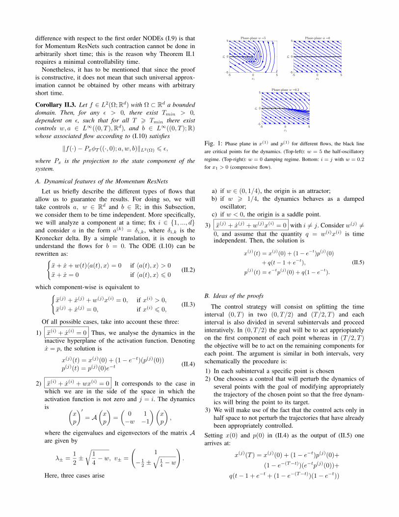
Fig. 1: Phase plane in x(1) and p(1) for different flows, the black lineare critical points for the dynamics. (Top-left): w = 5 the half-oscillatoryregime. (Top-right): w = 0 damping regime. Bottom: i = j with w = 0.2

for x1 > 0 (compressive flow).

a) if w ∈ (0, 1/4), the origin is an attractor;b) if w > 1/4, the dynamics behaves as a damped

oscillator;c) if w < 0, the origin is a saddle point.

3) x(j) + x(j) + w(j)x(i) = 0 with i 6= j. Consider w(j) 6=0, and assume that the quantity q = w(i)x(i) is timeindependent. Then, the solution is

x(j)(t) = x(j)(0) + (1− e−t)p(j)(0)

+ q(t− 1 + e−t),

p(j)(t) = e−tp(j)(0) + q(1− e−t).

(II.5)

B. Ideas of the proofs

The control strategy will consist on splitting the timeinterval (0, T ) in two (0, T/2) and (T/2, T ) and eachinterval is also divided in several subintervals and proceedinteratively. In (0, T/2) the goal will be to act appriopiatelyon the first component of each point whereas in (T/2, T )the objective will be to act on the remaining components foreach point. The argument is similar in both intervals, veryschematically the procedure is:1) In each subinterval a specific point is chosen2) One chooses a control that will perturb the dynamics of

several points with the goal of modifying appropriatelythe trajectory of the chosen point so that the free dynam-ics will bring the point to its target.

3) We will make use of the fact that the control acts only inhalf space to not perturb the trajectories that have alreadybeen appropriately controlled.

Setting x(0) and p(0) in (II.4) as the output of (II.5) onearrives at:

x(j)(T ) = x(j)(0) + (1− e−t)p(j)(0)+

(1− e−(T−t))(e−tp(j)(0))+

q(t− 1 + e−t + (1− e−(T−t))(1− e−t))

x(1)−axis

x(2)−axis

b

Controlled phase

Free phase

x+ x = q

x+ x = 0

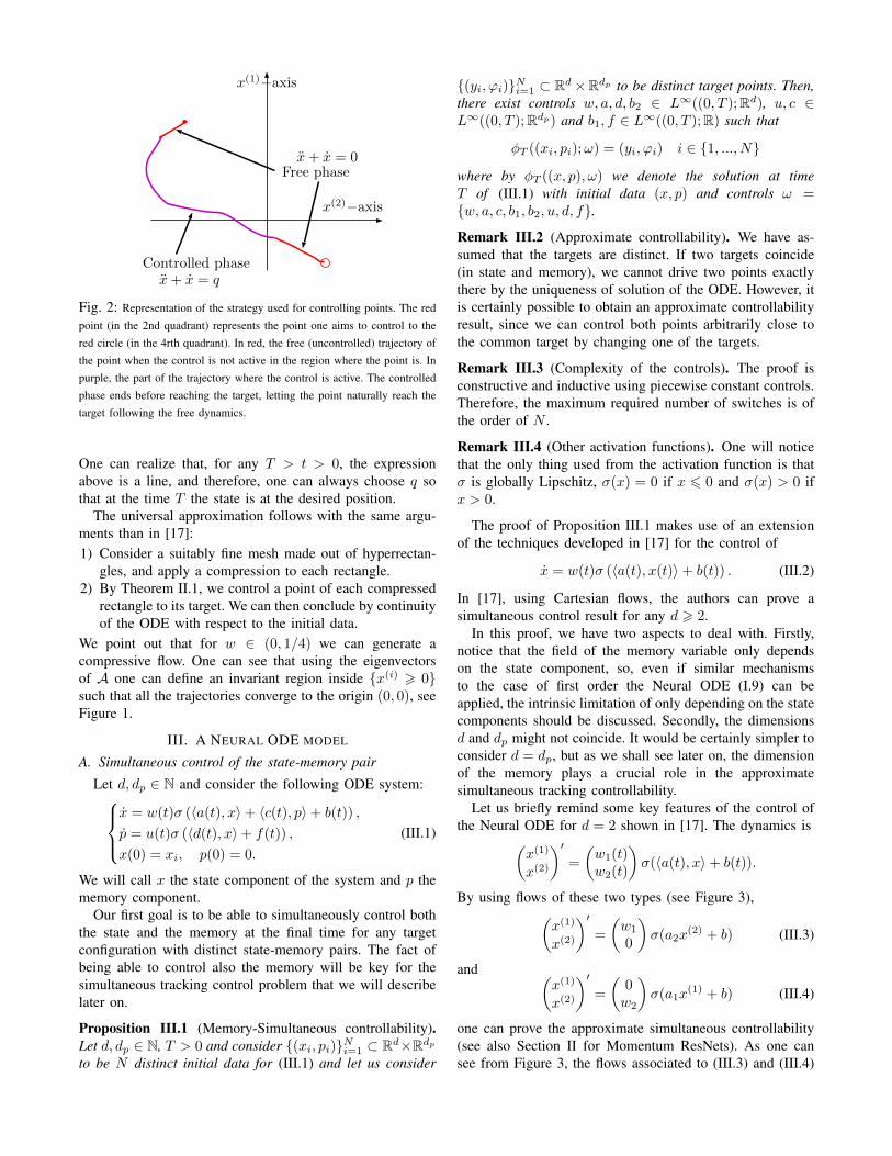
Fig. 2: Representation of the strategy used for controlling points. The redpoint (in the 2nd quadrant) represents the point one aims to control to thered circle (in the 4rth quadrant). In red, the free (uncontrolled) trajectory ofthe point when the control is not active in the region where the point is. Inpurple, the part of the trajectory where the control is active. The controlledphase ends before reaching the target, letting the point naturally reach thetarget following the free dynamics.

One can realize that, for any T > t > 0, the expressionabove is a line, and therefore, one can always choose q sothat at the time T the state is at the desired position.

The universal approximation follows with the same argu-ments than in [17]:1) Consider a suitably fine mesh made out of hyperrectan-

gles, and apply a compression to each rectangle.2) By Theorem II.1, we control a point of each compressed

rectangle to its target. We can then conclude by continuityof the ODE with respect to the initial data.

We point out that for w ∈ (0, 1/4) we can generate acompressive flow. One can see that using the eigenvectorsof A one can define an invariant region inside x(i) > 0such that all the trajectories converge to the origin (0, 0), seeFigure 1.

III. A NEURAL ODE MODEL

A. Simultaneous control of the state-memory pair

Let d, dp ∈ N and consider the following ODE system:x = w(t)σ (〈a(t), x〉+ 〈c(t), p〉+ b(t)) ,

p = u(t)σ (〈d(t), x〉+ f(t)) ,

x(0) = xi, p(0) = 0.

(III.1)

We will call x the state component of the system and p thememory component.

Our first goal is to be able to simultaneously control boththe state and the memory at the final time for any targetconfiguration with distinct state-memory pairs. The fact ofbeing able to control also the memory will be key for thesimultaneous tracking control problem that we will describelater on.

Proposition III.1 (Memory-Simultaneous controllability).Let d, dp ∈ N, T > 0 and consider (xi, pi)Ni=1 ⊂ Rd×Rdpto be N distinct initial data for (III.1) and let us consider

(yi, ϕi)Ni=1 ⊂ Rd×Rdp to be distinct target points. Then,there exist controls w, a, d, b2 ∈ L∞((0, T );Rd), u, c ∈L∞((0, T );Rdp) and b1, f ∈ L∞((0, T );R) such that

φT ((xi, pi);ω) = (yi, ϕi) i ∈ 1, ..., Nwhere by φT ((x, p), ω) we denote the solution at timeT of (III.1) with initial data (x, p) and controls ω =w, a, c, b1, b2, u, d, f.Remark III.2 (Approximate controllability). We have as-sumed that the targets are distinct. If two targets coincide(in state and memory), we cannot drive two points exactlythere by the uniqueness of solution of the ODE. However, itis certainly possible to obtain an approximate controllabilityresult, since we can control both points arbitrarily close tothe common target by changing one of the targets.

Remark III.3 (Complexity of the controls). The proof isconstructive and inductive using piecewise constant controls.Therefore, the maximum required number of switches is ofthe order of N .

Remark III.4 (Other activation functions). One will noticethat the only thing used from the activation function is thatσ is globally Lipschitz, σ(x) = 0 if x 6 0 and σ(x) > 0 ifx > 0.

The proof of Proposition III.1 makes use of an extensionof the techniques developed in [17] for the control of

x = w(t)σ (〈a(t), x(t)〉+ b(t)) . (III.2)

In [17], using Cartesian flows, the authors can prove asimultaneous control result for any d > 2.

In this proof, we have two aspects to deal with. Firstly,notice that the field of the memory variable only dependson the state component, so, even if similar mechanismsto the case of first order the Neural ODE (I.9) can beapplied, the intrinsic limitation of only depending on the statecomponents should be discussed. Secondly, the dimensionsd and dp might not coincide. It would be certainly simpler toconsider d = dp, but as we shall see later on, the dimensionof the memory plays a crucial role in the approximatesimultaneous tracking controllability.

Let us briefly remind some key features of the control ofthe Neural ODE for d = 2 shown in [17]. The dynamics is(

x(1)

x(2)

)′=

(w1(t)w2(t)

)σ(〈a(t), x〉+ b(t)).

By using flows of these two types (see Figure 3),(x(1)

x(2)

)′=

(w1

0

)σ(a2x

(2) + b) (III.3)

and (x(1)

x(2)

)′=

(0w2

)σ(a1x

(1) + b) (III.4)

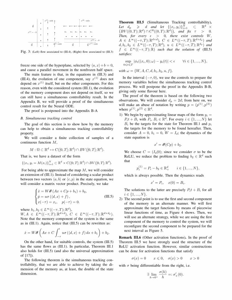
one can prove the approximate simultaneous controllability(see also Section II for Momentum ResNets). As one cansee from Figure 3, the flows associated to (III.3) and (III.4)

x(2)−axis

x(1) = −b

~0

~0x(1)−axis

x(2)−axis

x(2) = −b

~0~0x(1)−axis

Fig. 3: (Left) flow associated to (III.4), (Right) flow associated to (III.3)

freeze one side of the hyperplane, selected by 〈a, x〉+b = 0,and cause a parallel movement in the nonfrozen half space.

The main feature is that, in the equations in (III.3) and(III.4), the evolution of one component, say x(1) does notdepend on x(1) itself, but on the other components. For thisreason, even with the considered system (III.1), the evolutionof the memory component does not depend on itself, so wecan still have a simultaneous controllability result. In theAppendix B, we will provide a proof of the simultaneouscontrol result for the Neural ODE.

The proof is postponed into the Appendix B-A

B. Simultaneous tracking control

The goal of this section is to show how by the memorycan help to obtain a simultaneous tracking controllabilityproperty.

We will consider a finite collection of samples of acontinuous function M ,

M : Ω ⊂ Rd 7→ C([0, T ];Rd) ∩BV ([0, T ];Rd).

That is, we have a dataset of the form

(xi, yi = M(xi)Ni=1 ⊂ Rd × C([0, T ];Rd) ∩BV ([0, T ];Rd).

For being able to approximate the map M , we will consideran extension of (III.1). Instead of considering a scalar productbetween two vectors 〈a, b〉 or 〈c, p〉 in the state equation, wewill consider a matrix vector product. Precisely, we take

x = W~σ (Ax+ Cp+ b1) + b2,

p = uσ (〈d, x〉+ f) ,

x(−τ) = xi, p(−τ) = 0.

(III.5)

where b1, b2 ∈ L∞((−τ, T );Rd),W,A ∈ L∞((−τ, T );Rd×d), C ∈ L∞((−τ, T );Rd×dp).Note that the memory component of the system is the sameas in (III.1). Again, notice that (III.5) can be rewritten as:

x = W~σ

(Ax+ C

∫ t

−τuσ (〈d, x〉+ f) ds+ b1

)+ b2.

On the other hand, for suitable controls, the system (III.5)has the same flows as (III.1). In particular, Theorem III.1also holds for (III.5) (and also the universal approximationof [17]).

The following theorem is the simultaneous tracking con-trollability, that we are able to achieve by taking the di-mension of the memory as, at least, the double of the statedimension.

Theorem III.5 (Simultaneous Tracking controllability).Let dp > d and let (xi, yi)Ni=1 ⊂ Rd ×(BV ((0, T );Rd) ∩ C0((0, T );Rd)

), and fix τ > 0.

Then, for every ε > 0, there exist controls W ,A ∈ L∞((−τ, T );Rd×d), C ∈ L∞((−τ, T );Rd×dp) andd, b1, b2 ∈ L∞((−τ, T );Rd), u ∈ L∞((−τ, T );Rdp) andf ∈ L∞((−τ, T );R) such that the solution of (III.5)satisfies:

sup06t6T

|φt((xi, 0);ω)− yi(t)| < ε ∀i ∈ 1, ..., N,

with ω = W,A,C, d, b1, b2, u, f.In the interval (−τ, 0), we use the controls to prepare the

memory variables before the simultaneous tracking controlprocess. We will postpone the proof in the Appendix B-B,giving only some flavour here.

The proof of the theorem is based on the following twoobservations. We will consider dp = 2d; from here on, wewill make an abuse of notation by writing p = (p(1), p(2))where p(1), p(2) ∈ Rd.1) We begin by approximating linear maps of the form yi =

Pit+Bi with Pi, Bi ∈ Rd. For every i ∈ 1, ..., N letBi be the targets for the state for Theorem III.1 and pithe targets for the memory to be found hereafter. Then,consider A = 0, b1 = 0, W = Id; the dynamics of thestate equation is

x′ = ~σ(Cp) + b2.

We choose C = (Id|0); since we consider σ to be theReLU, we reduce the problem to finding b2 ∈ Rd suchthat

p(1)i = Pi − b2 ∈ Rd+ i ∈ 1, ..., N,

which is always possible. Then the dynamics reads

x′ = Pi, x(0) = Bi.

The solutions to the latter are precisely Pit+ Bi for alli ∈ 1, ..., N.

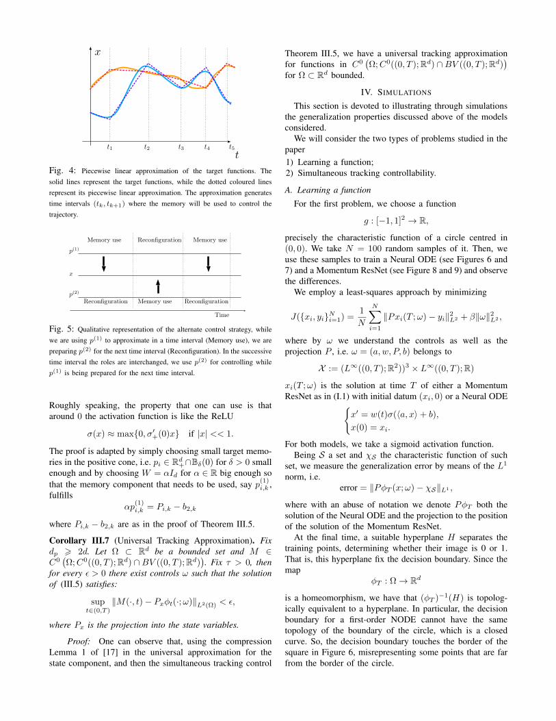
2) The second point is to use the first and second componentof the memory in an alternate manner. We will firstapproximate the target functions by means of piecewiselinear functions of time, as Figure 4 shows. Then, wewill use an alternate strategy, while we are using the firstcomponent of the memory to control the system, we willreconfigure the second component to be prepared for thenext interval as Figure 5.

Remark III.6 (Other activation functions). In the proof ofTheorem III.5 we have strongly used the structure of theReLU activation function. However, similar constructionscan be done for activation functions that satisfy

σ(x) = 0 x 6 0, σ(x) > 0 x > 0

with σ being differentiable from the right, i.e.

∃ limh→0+

σ(h)

h=: σ′+(0).

t

x

t1 t2 t3 t4 t5

Fig. 4: Piecewise linear approximation of the target functions. Thesolid lines represent the target functions, while the dotted coloured linesrepresent its piecewise linear approximation. The approximation generatestime intervals (tk, tk+1) where the memory will be used to control thetrajectory.

p(1)

p(2)

x

Memory use Reconfiguration

Reconfiguration ReconfigurationMemory use

Memory use

Time

Fig. 5: Qualitative representation of the alternate control strategy, whilewe are using p(1) to approximate in a time interval (Memory use), we arepreparing p(2) for the next time interval (Reconfiguration). In the successivetime interval the roles are interchanged, we use p(2) for controlling whilep(1) is being prepared for the next time interval.

Roughly speaking, the property that one can use is thataround 0 the activation function is like the ReLU

σ(x) ≈ max0, σ′+(0)x if |x| << 1.

The proof is adapted by simply choosing small target memo-ries in the positive cone, i.e. pi ∈ Rd+∩Bδ(0) for δ > 0 smallenough and by choosing W = αId for α ∈ R big enough sothat the memory component that needs to be used, say p(1)

i,k ,fulfills

αp(1)i,k = Pi,k − b2,k

where Pi,k − b2,k are as in the proof of Theorem III.5.

Corollary III.7 (Universal Tracking Approximation). Fixdp > 2d. Let Ω ⊂ Rd be a bounded set and M ∈C0(Ω;C0((0, T );Rd) ∩BV ((0, T );Rd)

). Fix τ > 0, then

for every ε > 0 there exist controls ω such that the solutionof (III.5) satisfies:

supt∈(0,T )

‖M(·, t)− Pxφt(·;ω)‖L2(Ω) < ε,

where Px is the projection into the state variables.

Proof: One can observe that, using the compressionLemma 1 of [17] in the universal approximation for thestate component, and then the simultaneous tracking control

Theorem III.5, we have a universal tracking approximationfor functions in C0

(Ω;C0((0, T );Rd) ∩BV ((0, T );Rd)

)for Ω ⊂ Rd bounded.

IV. SIMULATIONS

This section is devoted to illustrating through simulationsthe generalization properties discussed above of the modelsconsidered.

We will consider the two types of problems studied in thepaper1) Learning a function;2) Simultaneous tracking controllability.

A. Learning a function

For the first problem, we choose a function

g : [−1, 1]2 → R,

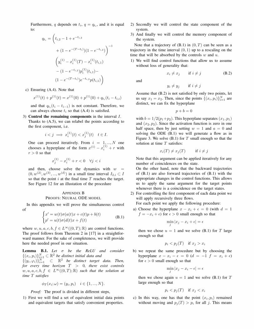
precisely the characteristic function of a circle centred in(0, 0). We take N = 100 random samples of it. Then, weuse these samples to train a Neural ODE (see Figures 6 and7) and a Momentum ResNet (see Figure 8 and 9) and observethe differences.

We employ a least-squares approach by minimizing

J(xi, yiNi=1) =1

N

N∑i=1

‖Pxi(T ;ω)− yi‖2L2 + β‖ω‖2L2 ,

where by ω we understand the controls as well as theprojection P , i.e. ω = (a,w, P, b) belongs to

X := (L∞((0, T );R2))3 × L∞((0, T );R)

xi(T ;ω) is the solution at time T of either a MomentumResNet as in (I.1) with initial datum (xi, 0) or a Neural ODE

x′ = w(t)σ(〈a, x〉+ b),

x(0) = xi.

For both models, we take a sigmoid activation function.Being S a set and χS the characteristic function of such

set, we measure the generalization error by means of the L1

norm, i.e.error = ‖PφT (x;ω)− χS‖L1 ,

where with an abuse of notation we denote PφT both thesolution of the Neural ODE and the projection to the positionof the solution of the Momentum ResNet.

At the final time, a suitable hyperplane H separates thetraining points, determining whether their image is 0 or 1.That is, this hyperplane fix the decision boundary. Since themap

φT : Ω→ Rd

is a homeomorphism, we have that (φT )−1(H) is topolog-ically equivalent to a hyperplane. In particular, the decisionboundary for a first-order NODE cannot have the sametopology of the boundary of the circle, which is a closedcurve. So, the decision boundary touches the border of thesquare in Figure 6, misrepresenting some points that are farfrom the border of the circle.

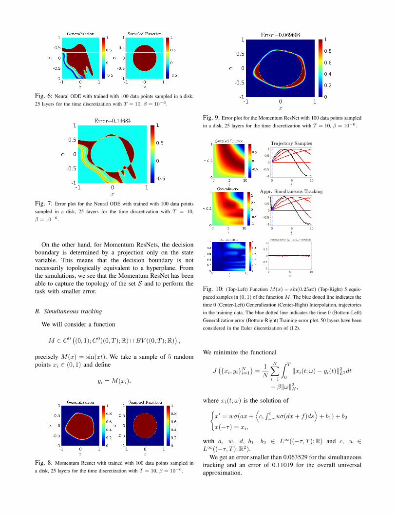
Fig. 6: Neural ODE with trained with 100 data points sampled in a disk,25 layers for the time discretization with T = 10, β = 10−6.

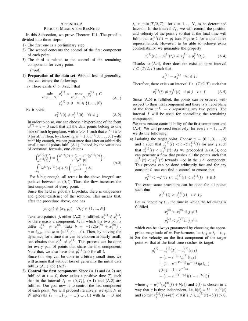
Fig. 7: Error plot for the Neural ODE with trained with 100 data pointssampled in a disk, 25 layers for the time discretization with T = 10,β = 10−6.

On the other hand, for Momentum ResNets, the decisionboundary is determined by a projection only on the statevariable. This means that the decision boundary is notnecessarily topologically equivalent to a hyperplane. Fromthe simulations, we see that the Momentum ResNet has beenable to capture the topology of the set S and to perform thetask with smaller error.

B. Simultaneous tracking

We will consider a function

M ∈ C0((0, 1);C0((0, T );R) ∩BV ((0, T );R)

),

precisely M(x) = sin(xt). We take a sample of 5 randompoints xi ∈ (0, 1) and define

yi = M(xi).

Fig. 8: Momentum Resnet with trained with 100 data points sampled ina disk, 25 layers for the time discretization with T = 10, β = 10−6.

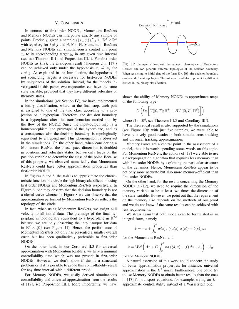
Fig. 9: Error plot for the Momentum ResNet with 100 data points sampledin a disk, 25 layers for the time discretization with T = 10, β = 10−6.

0 5 10-1

-0.5

0

0.5

1

0 5 10-1

-0.5

0

0.5

1

0 5 10-1

-0.5

0

0.5

1

0 5 10-1

-0.5

0

0.5

1

0 5 10-1

-0.5

0

0.5

1

Fig. 10: (Top-Left) Function M(x) = sin(0.25xt) (Top-Right) 5 equis-paced samples in (0, 1) of the function M . The blue dotted line indicates thetime 0 (Center-Left) Generalization (Center-Right) Interpolation, trajectoriesin the training data. The blue dotted line indicates the time 0 (Bottom-Left)Generalization error (Bottom-Right) Training error plot. 50 layers have beenconsidered in the Euler discretization of (I.2).

We minimize the functional

J(xi, yiNi=1

)=

1

N

N∑i=1

∫ T

0

‖xi(t;ω)− yi(t)‖2L2dt

+ β‖ω‖2X ,

where xi(t;ω) is the solution ofx′ = wσ(ax+

⟨c,∫ t−τ uσ(dx+ f)ds

⟩+ b1) + b2

x(−τ) = xi,

with a, w, d, b1, b2 ∈ L∞((−τ, T );R) and c, u ∈L∞((−τ, T );R2).

We get an error smaller than 0.063529 for the simultaneoustracking and an error of 0.11019 for the overall universalapproximation.

V. CONCLUSION

In contrast to first-order NODEs, Momentum ResNetsand Memory NODEs can interpolate exactly any sample ofpoints. Precisely, given a sample (xi, yi)Ni=1 ⊂ Rd × Rdwith xi 6= xj for i 6= j and d,N ∈ N, Momentum ResNetsand Memory NODEs can simultaneously control any pointxi to its corresponding target yi in any given time interval(see our Theorem II.1 and Proposition III.1). For first-orderNODEs as (I.9), the analogous result (Theorem 2 in [17])can be achieved only under the hypothesis yi 6= yj fori 6= j. As explained in the Introduction, the hypothesis ofnot coinciding targets is necessary for first-order NODEsby uniqueness of the solution. Instead, for the models in-vestigated in this paper, two trajectories can have the samestate variable, provided that they have different velocities ormemory states.

In the simulations (see Section IV), we have implementeda binary classification, where, at the final step, each poitis assigned to one of the two class according to a pro-jection on a hyperplan. Therefore, the decision boundaryis a hyperplane after the transformation carried out bythe flow of the NODE. Since the input-output map is ahomeomorphism, the preimage of the hyperplane, and asa consequence also the decision boundary, is topologicallyequivalent to a hyperplane. This phenomenon is observedin the simulations. On the other hand, when considering aMomentum ResNet, the phase-space dimension is doubledin positions and velocities states, but we only focus on theposition variable to determine the class of the point. Becauseof this property, we observed numerically that MomentumResNets could have better approximation properties thanfirst-order NODEs.

In Figures 6 and 8, the task is to approximate the charac-teristic function of a circle through binary classification usingfirst order NODEs and Momentum ResNets respectively. InFigure 6, one may observe that the decision boundary is nota closed curve whereas in Figure 8 we can observe that theapproximation performed by Momentum ResNets reflects thetopology of the circle.

In fact, when using Momentum ResNets, we assign nullvelocity to all initial data. The preimage of the final hy-perplane is topologially equivalent to a hyperplane in R2d

because we are only observing the intput-output for datain Rd × 0 (see Figure 11). Hence, the performance ofMomentum ResNets not only has presented a smaller overallerror, but has been qualitatively preferable to first-orderNODEs.

On the other hand, in our Corollary II.3 for universalapproximation with Momentum ResNets, we have a minimalcontrollability time which was not present in first-orderNODEs. However, we don’t know if this is a structuralproblem or if it is possible to prove this controllability resultfor any time interval with a different proof.

For Memory NODEs, we easily derived simultaneouscontrollability and universal approximation from the resultsof [17], see Proposition III.1. More importantly, we have

p−axis

x−axis

Decision boundary

Fig. 11: Example of how, with the enlarged phase-space of MomentumResNet, one can generate different topologies of the decision boundary.When restricting to initial data of the form R×0, the decision boundarycan have different topologies. The colors red and blue represent the differentclasses in the binary classification.

shown the ability of Memory NODEs to approximate mapsof the following type

C

(Ω;

[C([0, T ];Rd) ∩BV ([0, T ];Rd)

])where Ω ⊂ Rd, see Theorem III.5 and Corollary III.7.

The theoretical result is also supported by the simulations(see Figure 10): with just five samples, we were able tohave relatively good results in both simultaneous trackingand universal tracking approximation.

Memory issues are a central point in the assessment of amodel, thus it is worth spending some words on this topic.For Momentum ResNets, the authors of [18] were able to usea backpropagation algorithm that requires less memory thanwith first-order NODEs by exploiting the particular structureof the dynamics. Hence, Momentum ResNets appear to benot only more accurate but also more memory-efficient thanfirst-order NODEs.

On the other hand, for the results concerning the MemoryNODEs in (I.2), we need to require the dimension of thememory variable to be at least two times the dimension ofthe state variable. However, we point out that the requirementon the memory size depends on the methods of our proofand we do not know if the same results can be achieved withless requirements.

We stress again that both models can be formulated in anintegral form, namely

x = −x+

∫ t

0

w(s)σ (〈a(s), x(s)〉+ b(s)) ds

for the Momentum ResNet, and

x = W~σ

(Ax+ C

∫ t

0

uσ (〈d, x〉+ f) ds+ b1

)+ b2

for the Memory NODE.A natural extension of this work could concern the study

of better approximation properties, for instance, universalapproximation in the H1 norm. Furthermore, one could tryto use Memory NODEs to obtain better results than the onesin [17] for transport equations, for example, trying an L1-approximate controllability instead of a Wasserstein one.

APPENDIX APROOFS: MOMENTUM RESNETS

In this Subsection, we prove Theorem II.1. The proof isdivided into three steps.1) The first one is a preliminary step.2) The second concerns the control of the first component

of each point.3) The third is related to the control of the remaining

components for every point.Proof:

1) Preparation of the data set. Without loss of generality,one can ensure the following:

a) There exists C > 0 such that

mini∈1,...,N

x(1)i > max

j∈1,...,Ny

(1)j + C

p(1)i > 0 ∀i ∈ 1, ..., N

(A.1)

b) It holdsx

(1)i (0) 6= x

(1)j (0) ∀i 6= j (A.2)

In order to do so, one can choose a hyperplane of the formx(2) + b = 0 such that all the data points belong to oneside of such hyperplane, with b >> 1 such that x(2)

i +b >0 for all i. Then, by choosing ~w = (0, w(2), 0, . . . , 0) withw(2) big enough, we can guarantee that after an arbitrarilysmall time all points fulfil (A.1). Indeed, by the variationsof constants formula, one obtains(

x(1)(t)

p(1)(t)

)=

(x(1)(0) + (1− e−t)p(1)(0)

e−tp(1)(0)

)+∫ t

0

w(2)(x(2)(s) + b)

(1− es−t

es−t

)ds.

(A.3)

For b big enough, all terms in the above integral arepositive between in (0, t). Thus, the flow increases thefirst component of every point.Since the field is globally Lipschitz, there is uniquenessand global existence of the solution. This means that,after the procedure above, one has

(xi, pi) 6= (xj , pj) ∀i, j ∈ 1, ..., N.

Take two points i, j, either (A.2) is fulfilled, x(1)i 6= x

(1)j ,

or there exists a component, k, in which the two pointsdiffer x

(k)i 6= x

(k)j . Take b = −1/2(x

(k)i + x

(k)j ) ,

a = δk,k′ and w = (w(1), 0, ..., 0). Then, by solving thedynamics for a time that can be choosen arbitarly small,one obtains that x(1)

i 6= x(1)j . This process can be done

for every pair of points that share the first component.Note that, we also have that p(1)

l > 0 for all l.Since this step can be done in arbitrary small time, wewill assume that without loss of generality the initial datafulfills (A.1) and (A.2).

2) Control the first component. Since (A.1) and (A.2) arefulfilled at t = 0, there exists a positive time T1 suchthat in the interval I1 = (0, T1), (A.1) and (A.2) arefulfilled. Our goal now is to control the first componentof each point. We will proceed iteratively, we split I1 inN intervals I1 = ∪I1,i = ∪(ti−1, ti) with t0 = 0 and

ti < minT/2, T1 for i = 1, ..., N , to be determinedlater on. In the interval I1,i we will control the positionand velocity of the point i so that at the final time willfulfil that x(1)

i (T ) = yi (see Figure 2 for a qualitativerepresentation). However, to be able to achieve exactcontrollability, we guarantee the property

x(1)i (ti) + p

(1)i (ti) 6= x

(1)j + p

(1)j (tj). (A.4)

Thanks to (A.4), there does not exist an open intervalI ⊂ (T/2, T ) such that

x(1)i = x

(1)j ∀t ∈ I.

Therefore, there exists an interval I ⊂ (T/2, T ) such that

x(1)i (t) 6= x

(1)j (t) i 6= j t ∈ I. (A.5)

Since (A.5) is fulfilled, the points can be ordered withrespect to their first component and there is a hyperplaneof the form x(1) = c separating any two points. Theinterval I will be used for controlling the remainingcomponents.We now ensure controllability of the first component and(A.4). We will proceed iteratively; for every i = 1, ..., Nwe do the following:

a) Isolating the target point. Choose a = (0, 1, 0, . . . , 0)

and b such that x(1)i (t) < b < x

(1)j (t) for any j such

that x(1)i (t) < x

(1)j (t). As we proceeded in (A.3), one

can generate a flow that pushes all the points such thatx

(1)i (t) < x

(1)j (t) towards −∞ in the x(2) component.

This process can be done arbitrarily fast and for anyconstant C one can find a control to ensure that

p(2)j < −C ∀j s.t. x(1)

i (t) < x(1)j (t) t ∈ I1

The exact same procedure can be done for all pointssuch that

x(1)i (t) > x

(1)j (t) t ∈ I1.

Let us denote by ti,1 the time in which the following isfulfilled

x(2)j < x

(2)i if j 6= i

p(2)j < p

(2)i if j 6= i

which can be always guaranteed by choosing the appro-priate magnitude of w. Furthermore, let ti,2 = ti− ti,1.

b) Set the velocity on the first component of the targetpoint so that at the final time reaches its target.

y(1)i = x

(1)i (T ) = x

(1)i (ti,1)

+ (1− e−ti,2p(1)i (ti,1)

+ (1− e−(T−ti))e−ti,2)p(ti,1)

q(ti,2 − 1 + e−ti,2

+ (1− e−(T−ti))(1− e−ti,2))

where q = w(1)i (x

(2)i (t) + b(t)) and b(t) is chosen in a

way that q is time independent, i.e. b(t) = b∗ − x(2)i (t)

and so that x(2)j (t)+b(t) < 0 if j 6= i, x(2)

i (t)+b(t) > 0.

Furthermore, q depends on ti, q = qti , and it is equalto:

qti =

(ti,2 − 1 + e−ti,2

+ (1− e−(T−ti))(1− e−ti,2)

)−1

(y

(1)i − x

(1)i (T )− x(1)

i (ti,1)

− (1− e−ti,2)p(1)i (ti,1)−

(1− e−(T−ti))e−ti,2p(ti,1)

)c) Ensuring (A.4). Note that

x(1)(t) + p(1)(t) = x(1)(0) + p(1)(0) + qti(ti − ti,i)and that qti(ti − ti−1) is not constant. Therefore, wecan always choose ti so that (A.4) is satisfied.

3) Control the remaining components in the interval I .Thanks to (A.5), we can relabel the points according tothe first component, i.e.

i < j =⇒ x(1)i (t) < x

(1)j (t) t ∈ I.

One can proceed iteratively. From i = 1, ..., N onechooses a hyperplane of the form x(1) − x(1)

i + r withr > 0 so that

x(1)j − x

(1)i + r < 0 ∀j < i

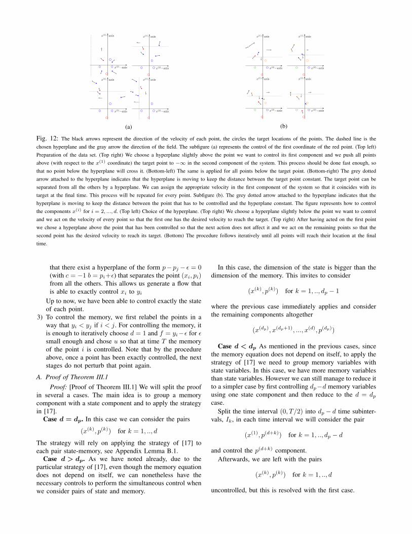
and then, choose solve the dynamics with w =(0, w(2), w(3), ..., w(d)) in a small time interval I2,i ⊂ Iso that the point i at the final time T reaches the target.See Figure 12 for an illustation of the procedure

APPENDIX BPROOFS: NEURAL ODE MODEL

In this appendix we will prove the simultaneous controlof

x′ = w(t)σ(a(t)x+ c(t)p+ b(t)

p′ = u(t)σ(d(t)x+ f(t)(B.1)

where w, u, a, c, b, f ∈ L∞((0, T );R) are control functions.The proof follows from Theorem 2 in [17] in a straightfor-ward manner. For the sake of completeness, we will providehere the needed proof in our situation.

Lemma B.1. Let σ be the ReLU and consider(xi, pi)Ni=1 ⊂ R2 be distinct initial data and(yi, ϕi)Ni=1 ⊂ R2 be distinct target data. Then,for every time horizon T > 0, there exist controlsw, u, a, c, b, f ∈ L∞((0, T );R) such that the solution attime T satisfies

φT (xi;ω) = (yi, pi) i ∈ 1, ..., N.

Proof: The proof is divided in different steps,1) First we will find a set of equivalent initial data points

and equivalent targets that satisfy convenient properties.

2) Secondly we will control the state component of thesystem.

3) And finally we will control the memory component ofthe system.

Note that a trajectory of (B.1) in (0, T ) can be seen as atrajectory in the time interval (0, 1) up to a rescaling on thetime that will be absorbed by the controls w and u.1) We will find control functions that allow us to assume

without loss of generality that:

xi 6= xj if i 6= j (B.2)

andyi 6= yj if i 6= j

Assume that (B.2) is not satisfied by only two points, letus say x1 = x2. Then, since the points (xi, pi)Ni=1 aredistinct, we can fix the hyperplane

p+ b = 0

with b = 1/2(p1+p2). This hyperplane separates (x1, p1)and (x2, p2). Since the activation function is zero in onehalf space, then by just setting w = 1 and a = 0 andsolving the ODE (B.1) we will generate a flow as inFigure 3. We solve (B.1) for T small enough so that thesolution at time T satisfies:

xi(T ) 6= xj(T ) if i 6= j

Note that this argument can be applied iteratively for anynumber of coincidences on the state.On the other hand, note that the backward trajectoriesof (B.1) are also forward trajectories of (B.1) with theappropriate changes in the control functions. This allowsus to apply the same argument for the target pointswhenever there is a coincidence on the target states.

2) For controlling the first component of each data point wewill apply recursively three flows.For each point we apply the following procedure:

a) Choose the hyperplane x − xi + ε = 0 (with d = 1f = −xi + ε) for ε > 0 small enough so that

minj|xj − xi + ε| = ε

then we chose u = 1 and we solve (B.1) for T largeenough so that

pi < pj(T ) if xj > xi

b) we repeat the same procedure but by choosing thehyperplane x − xi − ε = 0 (d = −1 f = xi + ε)for ε > 0 small enough so that

minj|xj − xi − ε| = ε

then we chose again u = 1 and we solve (B.1) for Tlarge enough so that

pi < pj(T ) if xj < xi

c) In this way, one has that the point (xi, pi) remainedwithout moving and pj(T ) > pi for all j. This means

x(1)−axis

x(2)−axisb

b

b

b

x(1)−axis

x(2)−axis

b

b

b

b

x(1)−axis

x(2)−axis

b

b

b

b

x(1)−axis

x(2)−axis

b

b

b

b

(a)

x(1)−axis

x(2)−axis

b

b

b

b

x(1)−axis

x(2)−axis

b

b

b

b

x(1)−axis

x(2)−axis

b

b

b

b

x(1)−axis

x(2)−axis

b

b

b

b

(b)

Fig. 12: The black arrows represent the direction of the velocity of each point, the circles the target locations of the points. The dashed line is thechosen hyperplane and the gray arrow the direction of the field. The subfigure (a) represents the control of the first coordinate of the red point. (Top left)Preparation of the data set. (Top right) We choose a hyperplane slightly above the point we want to control its first component and we push all pointsabove (with respect to the x(1) coordinate) the target point to −∞ in the second component of the system. This process should be done fast enough, sothat no point below the hyperplane will cross it. (Bottom-left) The same is applied for all points below the target point. (Bottom-right) The grey dottedarrow attached to the hyperplane indicates that the hyperplane is moving to keep the distance between the target point constant. The target point can beseparated from all the others by a hyperplane. We can assign the appropriate velocity in the first component of the system so that it coincides with itstarget at the final time. This process will be repeated for every point. Subfigure (b). The grey dotted arrow attached to the hyperplane indicates that thehyperplane is moving to keep the distance between the point that has to be controlled and the hyperplane constant. The figure represents how to controlthe components x(i) for i = 2, ..., d. (Top left) Choice of the hyperplane. (Top right) We choose a hyperplane slightly below the point we want to controland we act on the velocity of every point so that the first one has the desired velocity to reach the target. (Top right) After having acted on the first pointwe chose a hyperplane above the point that has been controlled so that the next action does not affect it and we act on the remaining points so that thesecond point has the desired velocity to reach its target. (Bottom) The procedure follows iteratively until all points will reach their location at the finaltime.

that there exist a hyperplane of the form p− pj − ε = 0(with c = −1 b = pi+ε) that separates the point (xi, pi)from all the others. This allows us generate a flow thatis able to exactly control xi to yi

Up to now, we have been able to control exactly the stateof each point.

3) To control the memory, we first relabel the points in away that yi < yj if i < j. For controlling the memory, itis enough to iteratively choose d = 1 and f = yi−ε for εsmall enough and chose u so that at time T the memoryof the point i is controlled. Note that by the procedureabove, once a point has been exactly controlled, the nextstages do not perturb that point again.

A. Proof of Theorem III.1Proof: [Proof of Theorem III.1] We will split the proof

in several a cases. The main idea is to group a memorycomponent with a state component and to apply the strategyin [17].

Case d = dp. In this case we can consider the pairs

(x(k), p(k)) for k = 1, .., d

The strategy will rely on applying the strategy of [17] toeach pair state-memory, see Appendix Lemma B.1.

Case d > dp. As we have noted already, due to theparticular strategy of [17], even though the memory equationdoes not depend on itself, we can nonetheless have thenecessary controls to perform the simultaneous control whenwe consider pairs of state and memory.

In this case, the dimension of the state is bigger than thedimension of the memory. This invites to consider

(x(k), p(k)) for k = 1, .., dp − 1

where the previous case immediately applies and considerthe remaining components altogether

(x(dp), x(dp+1), ..., x(d), p(dp))

Case d < dp As mentioned in the previous cases, sincethe memory equation does not depend on itself, to apply thestrategy of [17] we need to group memory variables withstate variables. In this case, we have more memory variablesthan state variables. However we can still manage to reduce itto a simpler case by first controlling dp−d memory variablesusing one state component and then reduce to the d = dpcase.

Split the time interval (0, T/2) into dp − d time subinter-vals, Ik, in each time interval we will consider the pair

(x(1), p(d+k)) for k = 1, .., dp − d

and control the p(d+k) component.Afterwards, we are left with the pairs

(x(k), p(k)) for k = 1, .., d

uncontrolled, but this is resolved with the first case.

B. Proof of Theorem III.5

Proof: [Proof of Theorem III.5] We will prove thetheorem for dp = 2d and this implies also the case dp > 2dby simply ignoring the dp−2d extra variables. We will dividethe proof in several steps1) Approximation. Consider a partition of (0, T ) by Nt

intervals Ik, (0, T ) = ∪Nt

k=1Ik so that every yi ∈C0((0, T );Rd) ∩ BV ((0, T );Rd) is approximated by apiecewise linear function. We consider the piecewiselinear function to be all of them linear in every Ik asFigure 4 shows. Let yhi be the approximation for yi andlet yhi,k be the function in the interval Ik

sup06t6T

|yi(t)− yhi | 6 ε i ∈ 1, ..., N

Furthermore, we can consider an approximation thatfulfills

∂x(1)yhi,k 6= ∂x(1)yhj,kif j 6= i k ∈ 1, ..., Nt. (B.3)

Thanks to (B.3) for every k there exist a subinterval Ik ⊂Ik such that(

yhi,k(x))(1)

6=(yhj,k(x)

)(1)

∀x ∈ Ik, if j 6= i, k ∈ 1, ..., Nt(B.4)

2) Simultaneous control. Now we apply Theorem III.1to approximately simultaneously control the state andthe memory. We choose for every i we choose yhi,1(0)as targets for the state component. The targets in thememory component will be chosen accordingly so thatthe dynamics

x′i = σ(Cpi) + b2

is able to reproduce the required linear trajectories. Wediscuss the target selection in the next step.

3) Alternating strategy. As we mentioned before, we willmake an abuse of notation and consider p = (p(1), p(2))with p(1), p(2) ∈ Rd. The strategy is visualised inFigure 5; we will use one component of the memoryto endow a linear movement while, in parallel, we willreconfigure the other component of the memory for theapproximation in the next interval. This requires to under-stand two things, first, which targets for the memory weshould select (Memory use) and second, how to controlthe component of the memory not used for controlling(Reconfiguration).

a) Use of the Memory. Let us consider the linear targetfunctions in Ik:

yhi,k = Bi,k + Pi,kt, i ∈ 1, ..., N,with Pi,k, Bi,k ∈ Rd. Consider A = 0, b1 = 0,W = Id,the dynamics of the state equation is

x′ = ~σ(Cp) + b2.

We choose Rd×dp 3 C = (Id|0) and we look formemory targets that are in the positive cone p(1)

i,kNi=1 ⊂Rd+. The activation function σ is assumed to be the

ReLU, and hence, we reduce the problem on findingb2,k ∈ Rd such that

p(1)i,k = Pi,k − b2,k ∈ Rd+ i ∈ 1, ..., N,

which is always possible. Then the dynamics triviallyreads

x′ = Pi,k, x(0) = Bi,k

whose solutions are Pi,kt+Bi,k for all i ∈ 1, ..., N.b) Reconfiguration. Since, for every k we have that there

exists an interval Ik for which (B.4) holds, one cancontrol the second component of the memory whilethe first component is used for following the trajectory.Thanks to (B.4) and the continuity of the trajectories,we can consider a subinterval

≈Ik such that, up to a

relabeling of the points we have(yhi,k)(1)

<(yhj,k)(1)

t ∈≈Ik, if i < j.

We set d = (1, 0, ..., 0) and we split≈Ik into N

subintervals, name them≈Ik,i and we proceed to control

the memory component that is not used to control thestate sequentially. Set

f(t) =(yhi,k(t)

)(1) − δfor δ > 0 small enough so that(

yhj,k(t))(1)

< f(t) t ∈≈Ik,i if j < i

We settle the memory targets for the next interval Ik+1

as in the previous step and then we choose

u = β (pi,k+1 − pi,k−1)

for β ∈ R so that when we solve the ODE

p′ = uσ(〈d, x〉+ f) t ∈≈Ik,i

the solution at tk,i := sup≈Ik,i satisfies that pi(tk,i) =

pi,k+1. Note that if j < i, the equation becomes

p′ = 0

so, once we have controlled the memory for one point,in the subsequent steps this memory will be unaltered.Therefore, we are able to exactly control the memorycomponent where we desire.

ACKNOWLEDGMENTS

We sincerely thank Carlos Esteve-Yague for his valuableconversations and comments.

This work has been funded by the European ResearchCouncil (ERC) under the European Union’s Horizon 2020research and innovation programme (grant agreement NO:694126-DyCon). The work of the third author is alsopartially supported by the Air Force Office of ScientificResearch (AFOSR) under Award NO: FA9550-18-1-0242, bythe Grant MTM2017-92996-C2-1-R COSNET of MINECO(Spain), by the Alexander von Humboldt-Professorship pro-gram, the European Unions Horizon 2020 research and

innovation programme under the Marie Sklodowska-Curiegrant agreement No.765579-ConFlex, and the Transregio 154Project “Mathematical Modelling, Simulation and Optimiza-tion Using the Example of Gas Networks” of the GermanDFG.

REFERENCES

[1] J. A. Barcena-Petisco. Optimal control for neural ode in a longtime horizon and applications to the classification and simultaneouscontrollability problems. 2021.

[2] R. T. Chen, Y. Rubanova, J. Bettencourt, and D. Duvenaud. Neuralordinary differential equations. arXiv preprint arXiv:1806.07366,2018.

[3] C. Cuchiero, M. Larsson, and J. Teichmann. Deep neural networks,generic universal interpolation, and controlled odes. SIAM Journal onMathematics of Data Science, 2(3):901–919, 2020.

[4] G. Cybenko. Approximation by superpositions of a sigmoidal function.Mathematics of control, signals and systems, 2(4):303–314, 1989.

[5] I. Daubechies, R. DeVore, S. Foucart, B. Hanin, and G. Petrova.Nonlinear approximation and (Deep) ReLU networks. ConstructiveApproximation, pages 1–46, 2021.

[6] C. Esteve, B. Geshkovski, D. Pighin, and E. Zuazua. Large-timeasymptotics in deep learning. arXiv preprint arXiv:2008.02491, 2020.

[7] I. Guhring and M. Raslan. Approximation rates for neural networkswith encodable weights in smoothness spaces. Neural Networks,134:107–130, 2021.

[8] E. Haber and L. Ruthotto. Stable architectures for deep neuralnetworks. Inverse Problems, 34(1):014004, 2017.

[9] K. He, X. Zhang, S. Ren, and J. Sun. Deep residual learning for imagerecognition. In Proceedings of the IEEE conference on computer visionand pattern recognition, pages 770–778, 2016.

[10] K. Hornik, M. Stinchcombe, and H. White. Multilayer feedforwardnetworks are universal approximators. Neural networks, 2(5):359–366,1989.

[11] A. Kolesnikov, L. Beyer, X. Zhai, J. Puigcerver, J. Yung, S. Gelly,and N. Houlsby. Big transfer (bit): General visual representationlearning. In Computer Vision–ECCV 2020: 16th European Conference,Glasgow, UK, August 23–28, 2020, Proceedings, Part V 16, pages491–507. Springer, 2020.

[12] Y. LeCun, Y. Bengio, and G. Hinton. Deep learning. nature,521(7553):436–444, 2015.

[13] Q. Li, T. Lin, and Z. Shen. Deep learning via dynamical systems: Anapproximation perspective. arXiv preprint arXiv:1912.10382, 2019.

[14] J.-L. Lions. Exact controllability, stabilization and perturbations fordistributed systems. SIAM review, 30(1):1–68, 1988.

[15] J. Loheac and E. Zuazua. From averaged to simultaneous controllabil-ity. In Annales de la Faculte des sciences de Toulouse: Mathematiques,volume 25, pages 785–828, 2016.

[16] A. Pinkus. Approximation theory of the mlp model in neural networks.Acta numerica, 8:143–195, 1999.

[17] D. Ruiz-Balet and E. Zuazua. Neural ode control for classification,approximation and transport, 2021.

[18] M. E. Sander, P. Ablin, M. Blondel, and G. Peyre. Momentum residualneural networks. arXiv preprint arXiv:2102.07870, 2021.

[19] E. Weinan. A proposal on machine learning via dynamical systems.Communications in Mathematics and Statistics, 5(1):1–11, 2017.

[20] C. E. Yague and B. Geshkovski. Sparse approximation in learning vianeural odes. arXiv preprint arXiv:2102.13566, 2021.

[21] M. Zhang, Z. McCarthy, C. Finn, S. Levine, and P. Abbeel. Learningdeep neural network policies with continuous memory states. In 2016IEEE international conference on robotics and automation (ICRA),pages 520–527. IEEE, 2016.