Embed Size (px)
Citation preview
Chapter 8
Function Interpolation andApproximation
We are now ready to study each step required for solving a Bellman equa-tion. For concreteness, let us write a problem here to refer to each of its
components in turn.
V (x, z) = max
y2�(x,z)
U(x, y) + �
ˆV (x0, z0)f(z0|z)dz0
�
s.t. x0= g(x, y, z)
Here, U(x, y) is the current period payoff as a function of the choice variable, y,and the endogenous state variable (possibly vector valued), x, of the problem. Itsevolution into x0 is described by the function g and depends on (x, y, z). Similarly, z
captures the exogenous, and here stochastic, state variable whose evolution is givenby the conditional density f(z0|z).
To maximize the right hand side, we need to first be able to evaluate the con-sequences of alternative choices y today for the value function tomorrow: V (x0, z0).But recall that we solve the Bellman equation on a discrete grid in today’s statevector, (xi, zj), which means that we only have a discrete table of values avail-able: V (xi, zj) for i = 1, .., n and j = 1, .., m. When maximizing the objective, itis typically best to let y be a continuous variable,1 which will also imply that x0
is a continuous variable, which in turn means that values of V (x0, ·) we try will
1There are various advantages to a continuous choice variable. Two advantages in particularare that (i) it allows us to use differentiable methods, such as first order conditions and Eulerequations, opening the door to very efficient algorithms, and (ii) typically it is much faster toperform maximization over a continuous space than a discrete grid, unless the latter is coarse, inwhich case, such discretization would seriously alter the original problem we would like to solveand is hence undesirable.
86
CHAPTER 8. FUNCTION INTERPOLATION AND APPROXIMATION 87
generically not land on the fixed grid for V 0. So, we will need to evaluate the valuefunction off the grid points—that is, we will need to interpolate. Second, if z is arandom variable with a continuous support—and, again, oftentimes we will assumethis to be the case—then to evaluate the integral, we will need to evaluate the valuefunction on a continuous interval of z0, this time requiring interpolation in thatdirection. Therefore, interpolation is a key tool we need to master for solving aBellman equation.
In this chapter, we will cover different methods for accomplishing this goal effi-ciently and accurately. As we shall see, interpolation can be a very difficult problemto deal with unless we are careful and learn the appropriate techniques.
8.1 Basic Idea
Suppose you are given a grid (x1
, x2,..., xn) and the function values (y
1
, y2
, ..., yn)
at corresponding points generated by function f(x). The problem of interpolationis to find an approximating function ˆf(x) that (i) agrees with f(x) at all grid pointsand (ii) provides a “good approximation” at all non-grid points within the domainof x. A “good approximation” is often taken to mean to minimize
�
�
�
f(x)� bf(x)�
�
�
according to some norm (Lp, sup-, etc). Notice that condition (i) and (ii) togetherabove is what makes this an interpolation rather than an approximation, which onlyrequires (ii).
In economics another very important concern is to preserve the shape—i.e.,concavity or convexity—of the interpolated (e.g, utility or value) function. As weshall see, some methods are especially good at guaranteeing that the shape of theinterpolant will also agree with the original function, while others are not.
Popular methods are linear-, Chebyshev-, and Spline- interpolations. I will spendmost of my time on Splines, because in the heterogeneous-agent model applicationsI have worked on, they often worked the best. Although linear interpolation lookstempting, given how easy it is to implement, it has some important drawbacks whichmakes it a last resort choice in many cases. More on this later.
8.2 Polynomial Interpolation
Polynomials provide a useful foundation for interpolation.2 However, their use re-quires much care. On the one hand, polynomials have some desirable properties,such as being smooth (differentiable), which allows their combination to approx-imate many differentiable functions well. One the other hand, they have some
2From Ralston and Rabinowitz:
CHAPTER 8. FUNCTION INTERPOLATION AND APPROXIMATION 88
drawbacks, such as being too smooth! What I mean is that the value of a polyno-mial anywhere in their domain (in fact over the complex plane) is determined by itsvalue in an arbitrarily small set. We can state and easily prove this assertion moreformally.
Theorem 8.1. Let p be an mth-order polynomial. Then p(x) is determined for allx 2 R by its values in any interval (a, b).
Proof. The proof is straightforward. Given any set of m points between a and b,i.e., a < t
1
< t2
< ... < tm < b, the polynomial p(x) is determined uniquely by itsvalues at these m points.
The implication is that if we try to fit the behavior of a function in a certain rangeof the real line, we determine the fate of the approximating polynomial everywhere.In this sense, polynomial approximations are very “global.” Thus, for example, ifthe function to be interpolated has some difficult features in a certain range, theinability to fit those features will affect the fitted function even far away from thatpoint. A well-known example of this problem is highlighted by the famous Rungeexample.
Theorem 8.2. [Runge] Let f(x) = 1/(1 + x2
) on [-5,5], and let Lmf be thepolynomial of order m that interpolates f at m equally-spaced points. Then:
lim sup
m!1|f(x)� Lmf | =
8
<
:
0 if |x| < 3.633...,
1 if |x| > 3.633...
Basically, this result says that the higher the order of the approximating func-tion, the larger is the error made by the interpolation off the grid points. And thefailure of the interpolation is not due to the function not being analytic—becauseit is. In fact, f is infinitely differentiable on R! Notice here of course that thenumber of grid points increases with the order (since this is interpolation) and theyare assumed to be equally spaced. It is possible to get better results by relaxingthese requirements. Still, this result is important for showing that going higherorder is not necessarily better when it comes to polynomial interpolations. In fact,Numerical Recipes (Press et al. (1992)) recommends, and I agree, that polynomialinterpolations that use powers in excess of 3 or 4 should be avoided.
So what to do then? As I said at the beginning, polynomials can be wonderfultools, we just have to know how to use them. One clever approach is provided bysplines.
CHAPTER 8. FUNCTION INTERPOLATION AND APPROXIMATION 89
8.3 Spline Interpolation
As noted in the previous section, polynomial interpolations typically do fine oversmall intervals, but they often produce wild oscillations when constructed over wideintervals, especially when the order is higher than 3 or 4. Polynomial splines arepiecewise polynomials that retain the smoothness of polynomials, but avoid itsimplication of wild oscillations at far away points by keeping the order low (typically2nd-4th degree) and breaking them into smaller intervals. In general, splines areextremely flexible constructs that can approximate functions that are very smooth(i.e., differentiable at high order) in certain parts of their domain and possiblycontain kinks and even jumps in other parts of their domain. A simple benchmark(that turns out to be sufficient for many economic applications) is the cubic splineinterpolation which I now discuss.3
Cubic Splines: Three Objectives
One of the most popular classes is cubic splines, and they satisfy three propertiesthat make them a good fit for economic applications. In particular a cubic splineinterpolant:
i. matches the function values at grid points (y1
, y2
, ..., yn) exactly (as with anyinterpolation).
ii. generates first derivatives that are continuous and differentiable for all x 2[x
1
, xn].
iii. generates second derivatives that are continuous for all values of x 2 [x1
, xn].
I now describe how to construct such splines and discuss issues related to their use.I include some further reading on the subject at the end of this chapter.
8.3.1 Building from Ground Up
Begin with the interval between two generic knots, xi and xi+1
. Begin by construct-ing a linear interpolant
y(x) = A(x)yj + B(x)yj+1
(8.3.1)
where
A(x) ⌘ xj+1
� x
xj+1
� xjand B(x) ⌘ 1� A =
x � xj
xj+1
� xj. (8.3.2)
3The theory of splines is very well developed and is widely used in engineering applicationssuch as 3D image processing and computer modeling among others. See, e.g., Schumaker (2007)and de Boor (2001) for detailed and authoritative treatments of the subject. Prenter (2008) isanother excellent source.
CHAPTER 8. FUNCTION INTERPOLATION AND APPROXIMATION 90
Although linear interpolation is sometimes useful, it has two important short-coming. One, the first derivative changes abruptly at the knot points, i.e., theinterpolant have as many kinks as the knot points. And two, the Second derivativedoes not exist at knot points. This can create many problems, such as difficultieswith derivative based minimization algorithms. So, how can we modify (8.3.1) toallow differentiable first derivatives and continuous second derivatives at all points?
Start by generalizing (8.3.1) using second derivative values at knot points:
y(x) = A(x)yj + B(x)yj+1
+ C(x)y00j + D(x)y00
j+1
(8.3.3)
whereC(x) =
1
6
(A3
(x)� A(x))(xj+1
� xj)2 (8.3.4)
andD(x) =
1
6
(B3
(x)� B(x))(xj+1
� xj)2. (8.3.5)
Note that you only need to know A and B to calculate everything. You caneasily verify that
d2y
dx2
= A(x)y00j + B(x)y00
j+1
.
Furthermore, since A(xj) = 1 and B(xj+1
) = 1 � A(xj+1
) = 1, the secondderivative agrees with y00
(x) at end points. But how to find y00j and y00
j+1
? First,differentiate (8.3.3) to obtain an expression for the first derivative of the interpolant:
dy
dx=
yj+1
� yj
xj+1
� xj� (xj+1
� xj)
6
�
(3A(x)2 � 1)y00j � (3B(x)2 � 1)y00
j+1
�
. (8.3.6)
This expression involves y00j and y00
j+1
. Recall that our second condition for theinterpolation was that the first derivative must be continuous throughout [x
1
, xn].Therefore, the two separate expressions for dy/dx obtained over the interval [xj , xj+1
]
and the interval [xj+1
, xj+2
] must equal each other at x = xj+1
. Rearranging theresulting expression yields
xj � xj�1
6
| {z }
cj�1
y00j�1
+
xj+1
� xj�1
3
| {z }
dj�1
y00j +
xj+1
� xj
6
| {z }
cj
y00j+1
=
yj+1
� yj
xj+1
� xj� yj � yj�1
xj � xj�1
| {z }
.
sj
�sj�1
(8.3.7)
For all interior knot points, j = 2, ..., n�1, we have an equation like this. Becausewe have n unknowns (y00
j for j = 1, ..., n), this system is underidentified. To obtain aunique solution we need to impose two boundary conditions. One sensible approachis to use the expression (8.3.6), which expresses the first derivative of the interpolantas a function of y00
j and y00j+1
and evaluate it at end points. By specifying the first
CHAPTER 8. FUNCTION INTERPOLATION AND APPROXIMATION 91
derivative at x1
and xn we obtain two more equations. Stacking n � 1 equationsfrom (8.3.7) and 2 equations from (8.3.6) to express them as a system of linearequations, we get:
2
6
6
6
6
6
6
6
6
6
6
6
6
4
2c1
�c1
c1
2d1
c2
. . .cj�1
2dj�1
cj
. . .cn�2
2dn�2
cn�1
�cn�1
2cn�1
3
7
7
7
7
7
7
7
7
7
7
7
7
5
.
2
6
6
6
6
6
6
6
6
6
6
6
6
4
y001
y002
...y00
j...
y00n�1
y00n
3
7
7
7
7
7
7
7
7
7
7
7
7
5
=
2
6
6
6
6
6
6
6
6
6
6
6
6
4
s1
� a⇤1
s2
� s1
...sj � sj�1
...sn�1
� sn�2
sn � a⇤n
3
7
7
7
7
7
7
7
7
7
7
7
7
5
.
(8.3.8)
C · pp = S
The matrix C depends only on the grid for x, whereas the vector of slopesS depends on the function values at grid points, as well as on the two boundaryconditions that we impose (a⇤
1
and a⇤n). This system of equations is not only linear,
but it is also tridiagonal: each unknown y00j is only linked to its two immediate
neighbors. Tridiagonal equations can be solved fairly efficiently, at rate O(N). Itcan also be parallelized fairly easily, which comes in handy when N is large.
An important question is whether the system of linear equations in (8.3.7) hasa unique solution for an arbitrary function f (alternatively put, for an arbitraryvector S). The answer depends on the nature of the boundary conditions that weimpose. For the particular ones chosen above—where we fixed the slopes at thetwo end points—the answer is yes. There are other boundary conditions that alsoensure that C is non-singular and therefore (8.3.7) has a unique solution. See forexample, Stoer and Bulirsch (2010, Theorem 2.4.2.13) for further details.
Once we obtain the solution vector, pp ⌘ ⇥
y001
, y002
, ..., y00N�1
, y00N
⇤
, we use equation(8.3.3) together with (8.3.2, 8.3.4, 8.3.5) to obtain the spline interpolation at anypoint x. Notice that the computation of coefficients A(x) to D(x) requires us tolocate x in the grid, that is, to find j such that xj x < xj+1
. This amounts tosearching an ordered table (x0
js) and can be done fairly efficiently. In the specialcase when the grid is equally-spaced, this is trivial. More generally, this can beachieved by bisection. However, oftentimes, we want to evaluate the interpolationat a vector of monotonically increasing abscissa values. In such cases, performingbisection for each abscissa is inefficient since we know that for each higher abscissathe index j will be higher than the one before.
CHAPTER 8. FUNCTION INTERPOLATION AND APPROXIMATION 92
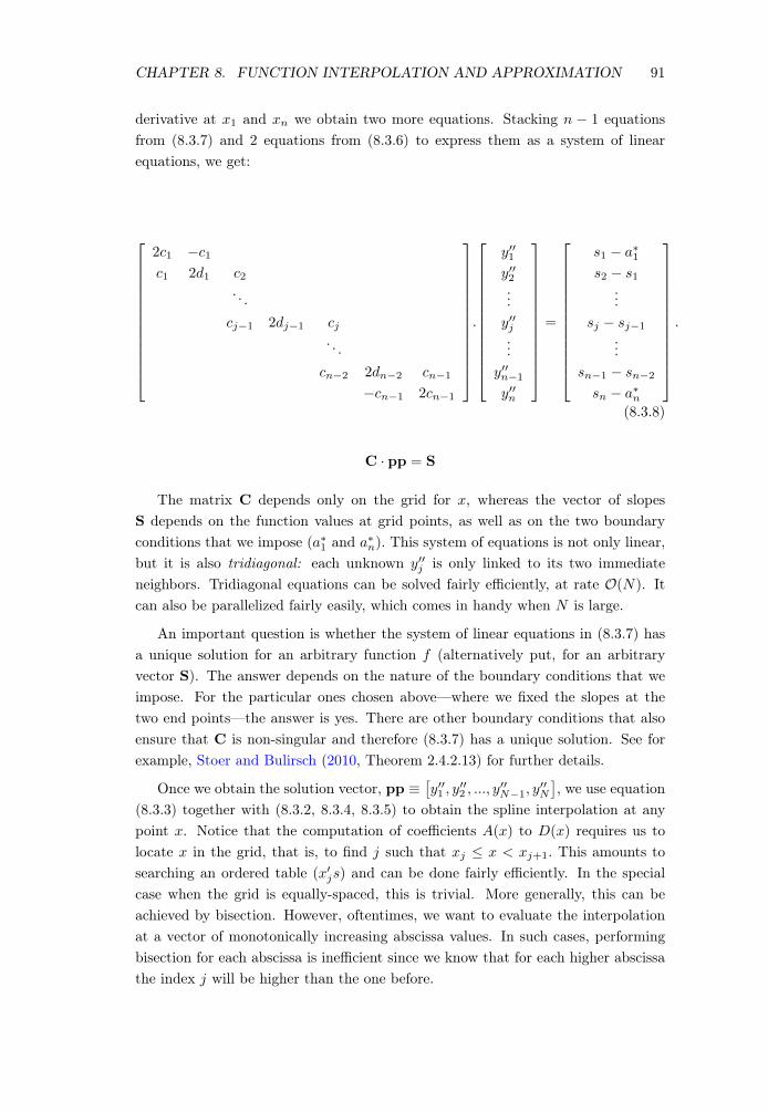
Figure 8.3.1 – Comparing Boundary Conditions for Cubic Spline
(a) N = 500 pts
0.04 0.06 0.08 0.1 0.12 0.14 0.16
Log
Axis
-1011
-1010
-109
-108
-107
-106
y′
1 = U′
(0.05)y
′
1 = 0Natural SplineTrue Function
(b) N = 100 pts
0.05 0.1 0.15 0.2 0.25
LinearAxis
×1010
-10
-5
0
5
y′
1 = U′
(0.05)y
′
1 = 0Natural splineTrue Function
8.3.2 Implementation
To summarize, implementing a spline interpolation has two distinct steps: (i) solvingfor the spline coefficients—the vector of y00
j s, and (ii) given coefficients, evaluatingthe interpolation at one or more abscissas. Some software implementations of cubicspline available (in online repositories, as well as in Matlab, etc.) provide programsthat combine the two steps into a single code as well as separate code for the twosteps. Unless you are careful it is easy (and my experience is that, it is often thecase) to do unnecessary computations.
This is why: The first step—solving for spline coefficients—is typically muchmore costly than the second, as it requires solving a system of linear equations.Although, this system is tridiagonal, it is still much more costly in computationaltime, especially when N is large. Furthermore, in some applications, the functionfor which we are constructing the interpolation will remain unchanged, but as thealgorithm evolves, we would be interested in evaluating the interpolation at abscis-sas that change. In such cases, it is essential to store the computed coefficientsobtained in step 1 once and then only execute the evaluation step as needed. Forexample, in Matlab calling Y Y = spline(X, Y, XX) executes both steps and re-turns the interpolated values at the vector of abscissas XX. However, if instead wecall PP = spline(X,Y ), the output are the spline coefficients, which can be storedand then used to evaluate Y Y = ppval(PP, XX) at any desired abscissa vector.Because spline interpolation is performed at the maximization step of the dynamicprogramming problem it is executed a very large number of times and inefficiencyat this step can cause the whole algorithm to be slow unnecessarily.
Setting Boundary Conditions. The boundary conditions should be set witha careful consideration of the shape of f . For example, for a power utility functionwith � > 1, the value function typically has a slope very close to zero at the top
CHAPTER 8. FUNCTION INTERPOLATION AND APPROXIMATION 93
end (f 0(xn)), so setting a⇤
n ⇡ 0 is a reasonable choice. At the low end, the slopeand the curvature are typically very high. One idea would be to set y0
1
> y02
sothat the slope continues to decline as x is increased (as is the case throughout U ’srange). But clearly this is infeasible, since y0
2
is only obtained after the interpolantis constructed whereas y0
1
must be set before it is constructed. One option is toset a⇤
1
= y01
=
y2�y1
x2�x1+ ", where " is a small positive number. Another option that
might work if f is a value function is to note the relationship between f and theunderlying utility function and use U 0
(x1
) to get a reasonable value for a⇤1
.
Boundary Conditions Matter. The particular choice of boundary values canmatter greatly in some applications. Figure 8.3.1a illustrates this point with anexample where the true function is a CRRA utility function with a RRA coefficientof 10. Three versions of the cubic spline interpolant is obtained by setting (i)y001
= 0 (so called “natural spline”), (ii) y01
= 0 (to illustrate a careless choice), and(iii) y0
1
= U 0(x
1
) (a sensible choice). The y-axis is in log scale to fit the wide range offunction values traced by the underlying function. As seen here, the first two choiceslead to large oscillations (considering the log nature of the y-axis), whereas the lastchoice provides an excellent fit even though every other detail of the implementationremained the same. The right panel (Figure 8.3.1b) slightly changes the exerciseby reducing the number of knot points from 500 in the left panel down to 100.Now the picture is reversed: imposing the correct first derivative at x
1
forces thespline interpolation to generate a very steep rise in the interpolated function, whichmatches the true function nicely at the very low end, but because the grid is chosento be coarse, the resulting interpolation yields much larger oscillations than theother two choices. However because none of the methods generate an acceptableinterpolation, the chosen grid is too coarse and must be made modified. We describealternative ways to achieve this below.
In short, the choice of boundary conditions affects the entire interpolant so theymust be set judiciously.
Cubic Spline Interpolation: Algorithm
It is useful to summarize the spline construction process.
What the Spline Interpolation Does Not Promise. A key point to note isthat no condition has been imposed for y0 or y00 to agree with the derivatives ofthe true function, f 0 and f 00, since the latter are unknown. The only condition isthat of “internal consistency”—that is, we require the spline interpolant constructedfor neighboring intervals to agree at knot points. As we shall see later, this is aweaker requirement than it may first appear and may lead to wild oscillations inthe interpolated values at not-a-knot points.
CHAPTER 8. FUNCTION INTERPOLATION AND APPROXIMATION 94
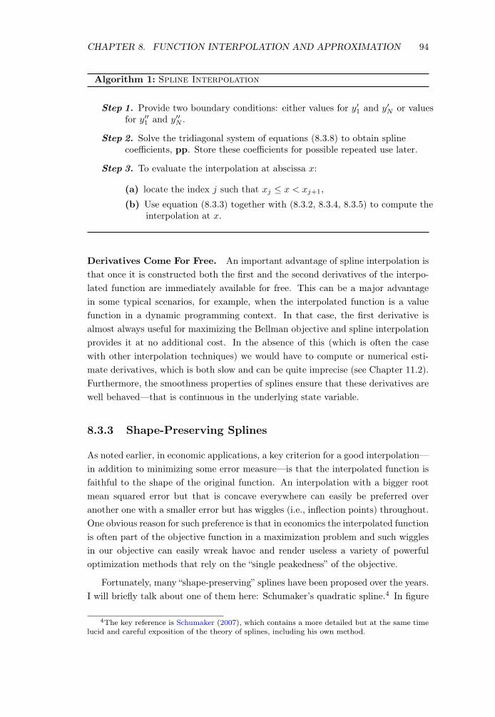
Algorithm 1: Spline Interpolation
Step 1. Provide two boundary conditions: either values for y01
and y0N or values
for y001
and y00N .
Step 2. Solve the tridiagonal system of equations (8.3.8) to obtain splinecoefficients, pp. Store these coefficients for possible repeated use later.
Step 3. To evaluate the interpolation at abscissa x:
(a) locate the index j such that xj x < xj+1
,
(b) Use equation (8.3.3) together with (8.3.2, 8.3.4, 8.3.5) to compute theinterpolation at x.
Derivatives Come For Free. An important advantage of spline interpolation isthat once it is constructed both the first and the second derivatives of the interpo-lated function are immediately available for free. This can be a major advantagein some typical scenarios, for example, when the interpolated function is a valuefunction in a dynamic programming context. In that case, the first derivative isalmost always useful for maximizing the Bellman objective and spline interpolationprovides it at no additional cost. In the absence of this (which is often the casewith other interpolation techniques) we would have to compute or numerical esti-mate derivatives, which is both slow and can be quite imprecise (see Chapter 11.2).Furthermore, the smoothness properties of splines ensure that these derivatives arewell behaved—that is continuous in the underlying state variable.
8.3.3 Shape-Preserving Splines
As noted earlier, in economic applications, a key criterion for a good interpolation—in addition to minimizing some error measure—is that the interpolated function isfaithful to the shape of the original function. An interpolation with a bigger rootmean squared error but that is concave everywhere can easily be preferred overanother one with a smaller error but has wiggles (i.e., inflection points) throughout.One obvious reason for such preference is that in economics the interpolated functionis often part of the objective function in a maximization problem and such wigglesin our objective can easily wreak havoc and render useless a variety of powerfuloptimization methods that rely on the “single peakedness” of the objective.
Fortunately, many “shape-preserving” splines have been proposed over the years.I will briefly talk about one of them here: Schumaker’s quadratic spline.4 In figure
4The key reference is Schumaker (2007), which contains a more detailed but at the same timelucid and careful exposition of the theory of splines, including his own method.
CHAPTER 8. FUNCTION INTERPOLATION AND APPROXIMATION 95
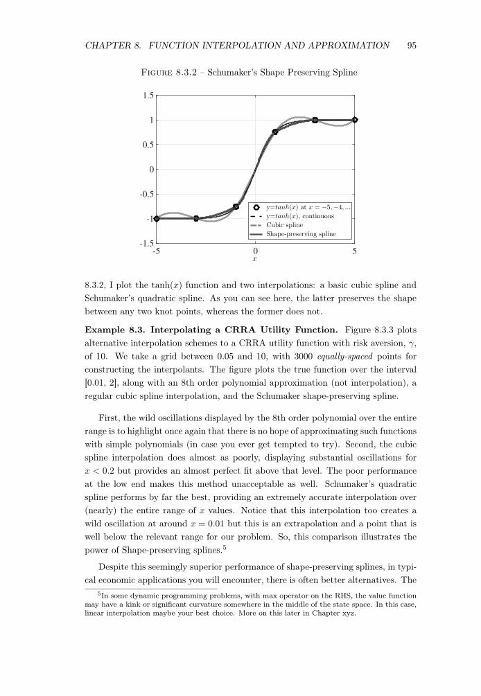
Figure 8.3.2 – Schumaker’s Shape Preserving Spline
x-5 0 5
-1.5
-1
-0.5
0
0.5
1
1.5
y=tanh(x) at x = −5,−4, ...y=tanh(x), continuousCubic splineShape-preserving spline
8.3.2, I plot the tanh(x) function and two interpolations: a basic cubic spline andSchumaker’s quadratic spline. As you can see here, the latter preserves the shapebetween any two knot points, whereas the former does not.
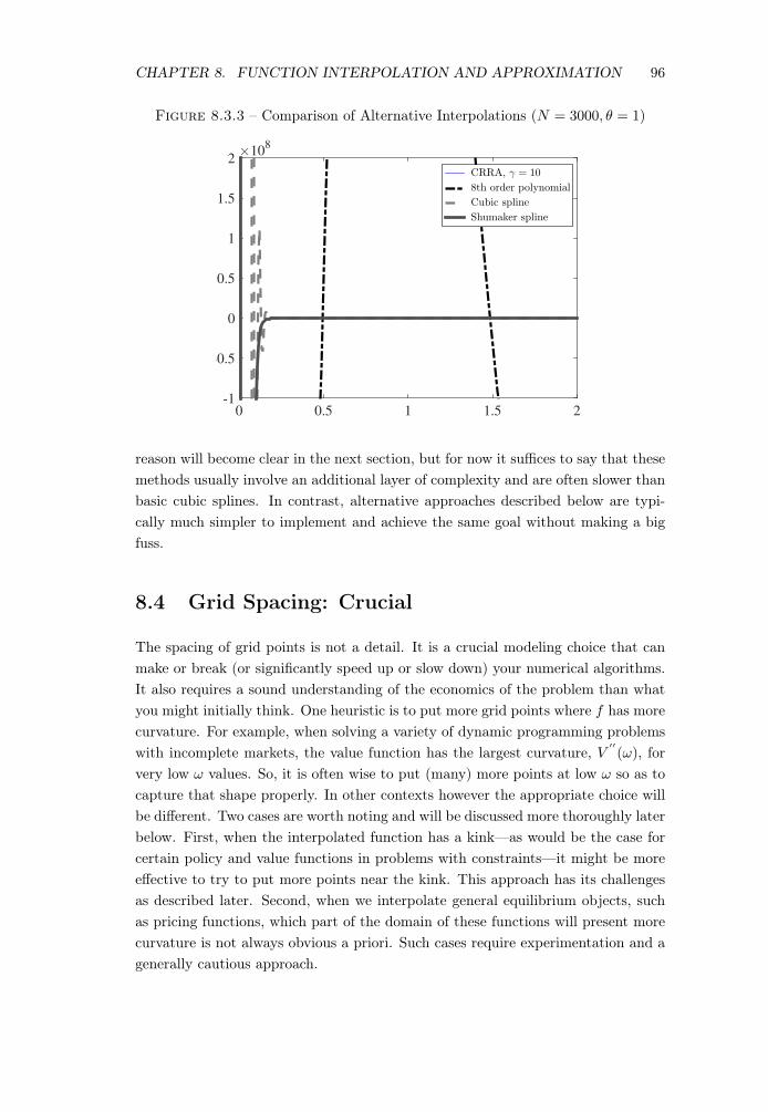
Example 8.3. Interpolating a CRRA Utility Function. Figure 8.3.3 plotsalternative interpolation schemes to a CRRA utility function with risk aversion, �,
of 10. We take a grid between 0.05 and 10, with 3000 equally-spaced points forconstructing the interpolants. The figure plots the true function over the interval[0.01, 2], along with an 8th order polynomial approximation (not interpolation), aregular cubic spline interpolation, and the Schumaker shape-preserving spline.
First, the wild oscillations displayed by the 8th order polynomial over the entirerange is to highlight once again that there is no hope of approximating such functionswith simple polynomials (in case you ever get tempted to try). Second, the cubicspline interpolation does almost as poorly, displaying substantial oscillations forx < 0.2 but provides an almost perfect fit above that level. The poor performanceat the low end makes this method unacceptable as well. Schumaker’s quadraticspline performs by far the best, providing an extremely accurate interpolation over(nearly) the entire range of x values. Notice that this interpolation too creates awild oscillation at around x = 0.01 but this is an extrapolation and a point that iswell below the relevant range for our problem. So, this comparison illustrates thepower of Shape-preserving splines.5
Despite this seemingly superior performance of shape-preserving splines, in typi-cal economic applications you will encounter, there is often better alternatives. The
5In some dynamic programming problems, with max operator on the RHS, the value functionmay have a kink or significant curvature somewhere in the middle of the state space. In this case,linear interpolation maybe your best choice. More on this later in Chapter xyz.
CHAPTER 8. FUNCTION INTERPOLATION AND APPROXIMATION 96
Figure 8.3.3 – Comparison of Alternative Interpolations (N = 3000, ✓ = 1)
0 0.5 1 1.5 2
×108
-1
-0.5
0
0.5
1
1.5
2CRRA, γ = 10
8th order polynomial
Cubic spline
Shumaker spline
reason will become clear in the next section, but for now it suffices to say that thesemethods usually involve an additional layer of complexity and are often slower thanbasic cubic splines. In contrast, alternative approaches described below are typi-cally much simpler to implement and achieve the same goal without making a bigfuss.
8.4 Grid Spacing: Crucial
The spacing of grid points is not a detail. It is a crucial modeling choice that canmake or break (or significantly speed up or slow down) your numerical algorithms.It also requires a sound understanding of the economics of the problem than whatyou might initially think. One heuristic is to put more grid points where f has morecurvature. For example, when solving a variety of dynamic programming problemswith incomplete markets, the value function has the largest curvature, V
00(!), for
very low ! values. So, it is often wise to put (many) more points at low ! so as tocapture that shape properly. In other contexts however the appropriate choice willbe different. Two cases are worth noting and will be discussed more thoroughly laterbelow. First, when the interpolated function has a kink—as would be the case forcertain policy and value functions in problems with constraints—it might be moreeffective to try to put more points near the kink. This approach has its challengesas described later. Second, when we interpolate general equilibrium objects, suchas pricing functions, which part of the domain of these functions will present morecurvature is not always obvious a priori. Such cases require experimentation and agenerally cautious approach.
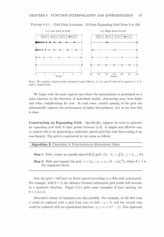
CHAPTER 8. FUNCTION INTERPOLATION AND APPROXIMATION 97
Figure 8.4.1 – Grid Point Locations: 51-Point Expanding Grid From 0 to 250
(a) Low End of Grid
Wealth
0 1 2 3 4 5
θ = 1 θ = 2 θ = 3 θ = 4
(b) High End of Grid
Wealth
220 225 230 235 240 245 250
θ = 1 θ = 2 θ = 3 θ = 4
Note: The number of grid points between 0 and 4.99 is 1, 8, 14, and 19 when ✓ is equal to 1, 2, 3,and 4, respectively.
We begin with the most typical case where the interpolation is performed on avalue function in the direction of individual wealth, abstracting away from kinksand other complications for now. In such cases, careful spacing of the grid cansubstantially improve the performance of spline interpolation. Let us see how thisis done.
Constructing an Expanding Grid. Specifically, suppose we need to generatean expanding grid with N knot points between [a, b]. A simple and effective wayto achieve this is by generating a uniformly spaced grid first and then scaling it upnon-linearly. The grid is constructed in two steps as follows.
Algorithm 2: Creating A Polynomially-Expanding Grid
Step 1. First, create an equally-spaced [0,1] grid: {x̃j : x̃j =
j�1
N�1
, j = 1, ..., N}.
Step 2. Shift and expand the grid: x = {xj : xj = a + (b � a)x̃j✓}, where ✓ > 1 is
the expansion factor.
Now the grid x will have its knots spaced according to a ✓th-order polynomial.For example, with ✓ = 2, the distance between subsequent grid points will increasein a quadratic function. Figure 8.4.1 plots some examples of knot spacing, for✓ = 1, 2, 3, 4.
Alternative forms of expansion are also possible. For example, in the first stepx̃ could be replaced with a grid from zero to ln(b � a + 1) and the second stepcould be replaced with an exponential function: xj = a + (ex̃
j � 1). This approach
CHAPTER 8. FUNCTION INTERPOLATION AND APPROXIMATION 98
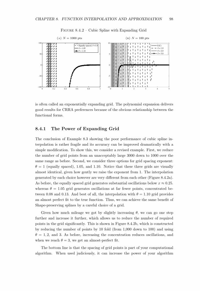
Figure 8.4.2 – Cubic Spline with Expanding Grid
(a) N = 1000 pts
0 0.2 0.4 0.6 0.8 1-100
-50
0
50
100
Equally-spaced, θ =1.0
θ = 1.05
θ = 1.10
(b) N = 100 pts
0 1 2 3 4 5-10
-5
0
5
10
U(C)
θ = 1.0
θ = 2.0
θ = 3.0
is often called an exponentially expanding grid. The polynomial expansion deliversgood results for CRRA preferences because of the obvious relationship between thefunctional forms.
8.4.1 The Power of Expanding Grid
The conclusion of Example 8.3 showing the poor performance of cubic spline in-terpolation is rather fragile and its accuracy can be improved dramatically with asimple modification. To show this, we consider a revised example. First, we reducethe number of grid points from an unacceptably large 3000 down to 1000 over thesame range as before. Second, we consider three options for grid spacing exponent:✓ = 1 (equally spaced), 1.05, and 1.10. Notice that these three grids are visuallyalmost identical, given how gently we raise the exponent from 1. The interpolationgenerated by each choice however are very different from each other (Figure 8.4.2a).As before, the equally spaced grid generates substantial oscillations below x ⇡ 0.25.whereas ✓ = 1.05 grid generates oscillations at far fewer points, concentrated be-tween 0.08 and 0.13. And best of all, the interpolation with ✓ = 1.10 grid providesan almost perfect fit to the true function. Thus, we can achieve the same benefit ofShape-preserving splines by a careful choice of a grid.
Given how much mileage we got by slightly increasing ✓, we can go one stepfurther and increase it further, which allows us to reduce the number of requiredpoints in the grid significantly. This is shown in Figure 8.4.2b, which is constructedby reducing the number of points by 10 fold (from 1,000 down to 100) and using✓ = 1, 2, and 3. As before, increasing the concentration reduces oscillations, andwhen we reach ✓ = 3, we get an almost-perfect fit.
The bottom line is that the spacing of grid points is part of your computationalalgorithm. When used judiciously, it can increase the power of your algorithm
CHAPTER 8. FUNCTION INTERPOLATION AND APPROXIMATION 99
significantly. So make sure not to waste the opportunity to use it effectively. Inthe examples studied here the utility function had a high curvature of � = 10.
With lower risk aversion, one could use as few as 50 grid points, and a value of✓ between 2 and 3 without generating any undesirable oscillations. However, it iscritical to conduct an exercise such as the one presented here to develop a senseabout your particular application. It is also advisable to use a denser grid (i.e., withmore points than necessary, perhaps with 200 or 300 points) at the early stages ofthe programming process (when you are still building, testing, and debugging yourcode). Once you are confident that everything works well, you can gradually reducethe number of points to increase speed, while carefully watching for any potentialproblems along the way.
Before concluding, a remark is in order. While putting more grid points at thelow end is often wise for individual state variables, such as wealth or cash-in-hand,this is not a hard and fast rule, especially for knot placement for aggregate statevariables. For example, in a dynamic macro model (e.g., an RBC style framework)in which capital does not fluctuate too much, you may want to place more gridpoints near the mean, K, even though the functions of interest may have morecurvature at low K values.
Exercise 8.4. Illustrate the differences between interpolating using Chebyshev,linear, and Spline interpolation by showing how each one fits a utility function withrisk aversion of 10. I found in the past that you need Chebyshev polynomial with130th power to fit this utility function.
8.5 A Trick to Reduce the Curvature
The various interpolation methods presented so far aim to approximate functionswith high curvature by a combination of clever techniques and some brute force (e.g.,take lots of grid points). An orthogonal approach to the same problem proceedsby representing the same function with one that has lower curvature and thereforeis easier to interpolate to begin with. To see how this works, it is useful to reviewsome basic results on the curvature of value functions.
Recall from Chapter 3.2 that the Merton-Samuelson theorem (Theorem 3.3) es-tablishes that with CRRA preferences and a linear budget set (e.g., as in a standardportfolio choice problem), the value function inherits the curvature of U , that is,V (!,A) = �(A)⇥ !1�� , where ! denotes wealth, A represents the vector of statevariables other than wealth, and � is risk aversion. The same result holds approxi-mately true in a variety of different problems. With incomplete markets V (w) willtypically have even more curvature than U(c), especially at low wealth levels. Aswe have seen so far, when � is large, this high curvature creates a lot of headachewhen you try to interpolate the value function. Fortunately, there is a way out.
CHAPTER 8. FUNCTION INTERPOLATION AND APPROXIMATION 100
To see how, consider this an alternative formulation of CRRA preferences:
U(c0
, c1
, ...) =
1X
t=1
�tc1��t
!
1/(1��)
, (8.5.1)
which is simply a CES aggregator of the entire consumption stream.6 This speci-fication is ordinally equivalent to, and thus represents the same preferences, as theusual CRRA formulation:
P1t=1
�t c1��
t
1�� . However, there is a key difference when itcomes to the shape of the resulting value function, which is now linear in wealth:
V (!, A) = �(A)⇥ !.
Although incomplete markets introduces some curvature (very little in fact andconcentrated at the very low levels of !), this value function is still much easier tointerpolate than the one above. This is a relatively little known trick, but it cansave you a lot of time and headache.
8.5.1 Implementation
Consider the following consumption-savings problem with Epstein-Zin preferences:
V (k; y) =max
c,k0
h
(1� �) c1��+ �E(V (k0
; y0)
1�� |y)i
11��
(8.5.2)
s.t. c + k0 (1 + r)k + y,
y0= ⇢y + ⌘,
k0 � k.
Now take a look at Figure 8.5.1, which plots the utility function of this Bellmanequation under the standard CRRA parameterization with � = 10 and under thealternative in (8.5.1). The standard CRRA representation has two problems. First,at the low end, there is enormous curvature as seen here (dashed line with squaremarkers—plotted on a logarithmic scale to fit the substantial variation in the valuefunction). One reaction might be that maybe we should scale up the problem so thelowest reasonable consumption value is not too small, say, around 1 instead of 0.05chosen here. But the this will exacerbate the second problem with CRRA—thatthe utility function gets too flat at the top end. Scaling up the x -axis by 10-fold,for example, to fix the first problem results in the utility function getting closer tozero by 1010 at the top end. Alternatively, if we decide to shrink the interval thatalso creates similar problems. The bottom line is that CRRA raises consumption
6Notice that this is a special case of Epstein-Zin preferences (obtained by setting risk aversionto the inverse of the EIS), which was discussed in detail in Chapter 5.3.
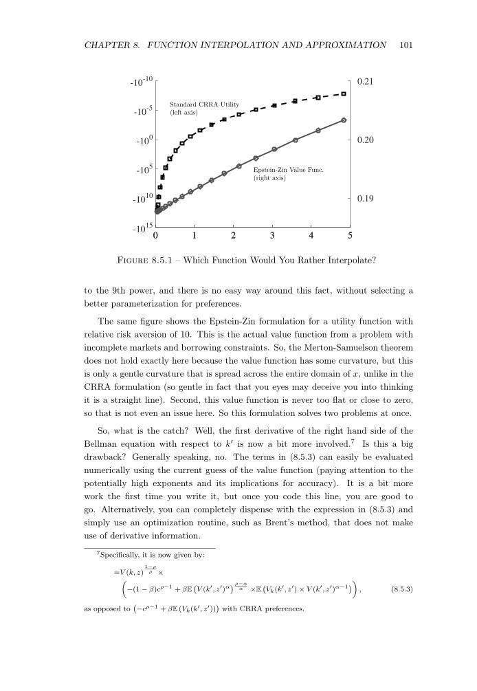
CHAPTER 8. FUNCTION INTERPOLATION AND APPROXIMATION 101
0 1 2 3 4 5-10
15
-1010
-105
-100
-10-5
-10-10
0 1 2 3 4 5
0.19
0.20
0.21
Epstein-Zin Value Func.(right axis)
Standard CRRA Utility(left axis)
Figure 8.5.1 – Which Function Would You Rather Interpolate?
to the 9th power, and there is no easy way around this fact, without selecting abetter parameterization for preferences.
The same figure shows the Epstein-Zin formulation for a utility function withrelative risk aversion of 10. This is the actual value function from a problem withincomplete markets and borrowing constraints. So, the Merton-Samuelson theoremdoes not hold exactly here because the value function has some curvature, but thisis only a gentle curvature that is spread across the entire domain of x, unlike in theCRRA formulation (so gentle in fact that you eyes may deceive you into thinkingit is a straight line). Second, this value function is never too flat or close to zero,so that is not even an issue here. So this formulation solves two problems at once.
So, what is the catch? Well, the first derivative of the right hand side of theBellman equation with respect to k0 is now a bit more involved.7 Is this a bigdrawback? Generally speaking, no. The terms in (8.5.3) can easily be evaluatednumerically using the current guess of the value function (paying attention to thepotentially high exponents and its implications for accuracy). It is a bit morework the first time you write it, but once you code this line, you are good togo. Alternatively, you can completely dispense with the expression in (8.5.3) andsimply use an optimization routine, such as Brent’s method, that does not makeuse of derivative information.
7Specifically, it is now given by:
=V (k, z)1�⇢
⇢ ⇥✓�(1� �)c⇢�1
+ �E�V (k0, z0)↵
� ⇢�↵
↵ ⇥E�Vk
(k0, z0)⇥ V (k0, z0)↵�1
�◆, (8.5.3)
as opposed to��c⇢�1
+ �E (Vk
(k0, z0))�
with CRRA preferences.
CHAPTER 8. FUNCTION INTERPOLATION AND APPROXIMATION 102
8.5.2 Extrapolation
Never extrapolate. If you must, do not extrapolate too far beyond the last gridpoint (e.g., no more than � ⌘ xN � xN�1
). If you absolutely must extrapolate far,use a low order method such as a blending of linear interpolation. And check theworst case scenarios, such as if the extrapolation leads to an answer that has thewrong sign and such. But like I said, never extrapolate.
Or avoiding too much curvature as you determine the boundary condition forspline.
8.6 Taking Stock
For any model that you solve, you must eventually re-solve it on a much finer gridand confirm that your main results are not changing (much). This is the only realis-tic way to check if approximation errors coming from interpolations are important.You will be surprised to find that some bad-looking interpolations actually yield thesame results as much more accurate (and more costly to compute) interpolations.And vice versa. Some problems are especially sensitive to any kind of approximationerrors. We will see examples, especially in asset pricing.
Regarding splines, what I especially like about them—compared with other in-terpolation techniques, such as Chebyshev or other polynomial methods—is thatsplines give us enormous freedom in where we put the knot points. This is very lib-erating because in many cases there is as much economics involved in making thatchoice as there is knowledge of computational techniques. In contrast Chebyshevand other methods are not designed to cope with such concerns and rely entirely onassumptions about the geometry of the function to be evaluated. For example, if Iknow that there is almost zero chance that individuals will visit a given part of thestate space, I might want to be a tad more flexible in accepting less accuracy there.This is purely a judgement call and is based on aspects of the economic problemthat Chebyshev is blind to. Of course, this only works, if I apply good judgement,which requires a very good understanding of the economic problem.
A Word About B-Splines
This chapter has presented the basic method of cubic spline interpolation, whichis an (important) special case of the much broader theory of splines. The gen-eral theory is extremely flexible allowing accurate interpolation of high-dimensionalsurfaces, whose smoothness can vary drastically across its shape (being highly differ-entiable in some areas and displaying kinks in others). This more general theory ismore conveniently developed under an alternative formulation which builds splines
CHAPTER 8. FUNCTION INTERPOLATION AND APPROXIMATION 103
from a set of basis functions, called B-splines, which are polynomials that are non-zero only over a finite interval and zero everywhere else. In addition to providing aflexible foundation construction of spline interpolation via B-splines can also lead tosignificant gains in computational efficiency. de Boor (2001) provides the followingresult, which illustrates this point.
Theorem. Constructing a cubic spline interpolation with (m, n) points in (x, y)
direction requires:
u O((mn)3) operations using regular splines.
u O(m3
+ m2n + mn2
+ n3
) operations with B-splines.
To understand the difference, suppose m = n = 10. Then regular spline requiresabout one million operations, whereas B-splines require only about 4,000 operations!Although a detailed treatment of the theory of B-splines is beyond the scope of thisbook, the interested reader is encouraged to consult the classic text by de Boor(2001) (which provides a detailed and authoritative treatment of spline theory).Schumaker (2007) is another excellent source with a lucid exposition of the topic andPrenter (2008) contains a detailed treatment of multi-dimensional tensor productB-splines.
8.7 Exercises
Exercise 8.5. This problem asks you to interpolate some utility functions usingthree different methods. Do not use the built-in routines in MatLab or other high-level programming languages. The goal is for you to understand how each of thesemethods works. You may copy and paste algorithms from Numerical Recipes though(even into MatLab and then modify the syntax). Specifically, write programs forinterpolating values of the utility functions given below:
u(c) = log(c)
u(c) =p
c
u(c) =c1�↵
1� ↵, for ↵ = 2, 5, 10.
Suppose that you can evaluate these functions at as many points as necessary overthe domain [0.05, 2]. So how many points you choose to perform the interpolationis up to you, but you should aim to minimize the computational burden (i.e., asfew function evaluations as possible). Assess the accuracy of each interpolationscheme in intervals of .05. Plot the function and what results from using eachapproximation.
CHAPTER 8. FUNCTION INTERPOLATION AND APPROXIMATION 104
Exercise 8.6. Optimal Choice of ✓. An interesting question raised by the precedingdiscussion is if there is an optimal way to choose ✓ in a given problem. To makethe question more concrete, suppose that our goal is to interpolate a CRRA utilityfunction with a given curvature � and we choose a goodness-of-fit statistic, such asthe sup-norm in percentage deviation terms to be less than a small number toler(say 10
�5). What is the minimum required ✓ that would deliver this accuracy withN grid points? One can write a computer program to solve this problem.
Exercise 8.7. Conduct the experiment using (i) linear interpolation, (ii) cubicsplines, (iii) Chebyshev polynomials. The first two interpolation schemes allow youto choose grid points any way you like. Make an educated guess about how youshould space the grid points to minimize computational cost for a given level ofaccuracy. Which interpolation scheme works the best, in terms of minimizing thecomputational burden? In case of (i) and (ii) how many points do you need to takeso that your maximum error is less than 1% of the function value at each point?Experiment with different ways to space your points. In case of (iii) what is theorder of Cheb. Pols. you need for the desired accuracy?
Exercise 8.8. The perils of extrapolation. Now we will extrapolate: calculate thevalue of each utility function at c = 0.02 and c = 2.1, 2.5, and 4 using the differentinterpolation schemes. Is this feasible for all three methods above? Among thefeasible ones, which one works better for extrapolation?
Exercise 8.9. Write a program (in Matlab or Fortran) to solve the neoclassicalgrowth model by iterating on the value function, but rather than restricting capitalto a discrete grid as in the fourth problem on Homework #1, instead approximatethe value function by a cubic spline. That is, pick a grid of points (centered on thesteady-state capital stock) at which to keep track of the value function, but do notrestrict choices for tomorrow’s capital to this grid. When searching for the optimalchoice for tomorrow’s capital (i.e., the value of tomorrow’s capital that maximizesthe right-hand side of Bellman’s equation, given the current value of capital), usecubic spline interpolation to compute the value function off the grid. Report resultsfor both full depreciation and less-than-full depreciation. Compare your results tothe analytical solution (for the case of full depreciation) and to the results that youfound in the fourth problem of Homework #1.
Exercise 8.10. This question will teach you about a different parameterizationof CRRA utility functions that yields an approximately linear value function ina wide-range of economic problems. This approximate linearity will save you asubstantial amount of time when you solve DP problems and need to interpolatethe value function on the RHS. First, some preliminaries. This part asks you to dosome algebra to get acquainted with Epstein-Zin preferences.
a. Consider a basic portfolio choice problem where preferences are given by theEpstein-Zin specification (also called “recursive preferences”). For the specifics
CHAPTER 8. FUNCTION INTERPOLATION AND APPROXIMATION 105
of this problem, see Epstein (1988). Derive the relative risk aversion coefficientwith respect to wealth gambles, that is �W ((J
00(W ))/(J
0(W ))) (where W is
financial wealth and J(.) is the value function) and show that it is equal to(1/(1� ↵)) where a is the exponent of future utility.
b. Now, we will modify the problem a bit. Suppose that there is a single risk-free asset for investment subject to an ad hoc borrowing constraint (in thelanguage of Aiyagari (1994)). Furthermore, suppose that the individual re-ceives a stochastic labor income that follows a first order Markov process witha bounded support (again as in Aiyagari). Solve the dynamic programmingproblem of the individual numerically using value function iteration. Repeatthe experiment for risk aversion coefficient of 2, and 10, and EIS values of2, and 0.1. [Discussion: When you do value function iteration you will needto interpolate the value function next period (i.e., on the right hand side ofthe Bellman equation) at the off-grid points. You are free to use any kindof interpolation technique as you wish as long as you minimize the compu-tational time necessary. If you feel like it, experiment with different choices(linear, spline, and Chebyshev) and report which one works best (in termsof delivering an accurate solution in as little time as possible). You shoulditerate until the discrepancy in the decision rule between successive iterations(under sup-norm) is less than 10
�8. Finally, you should use a maximizationroutine that makes use of derivative information (such as Dbrent.f90 or someNewton-based algorithm for efficiency. In both cases, make sure to supply thecorrect analytical derivative of the right hand side of the Bellman equation,which is a bit more involved than with CRRA specification.
c. Plot the decision rules and value function as a function of individual’s financialwealth keeping his income shock constant at its average value.
d. Now set the parameters of the Epstein-Zin specification such that it reducesto standard CRRA utility. Solve the problem in part (b) again taking a riskaversion value of 2. Repeat with RRA= 10.
e. Now solve the portfolio choice problem in (d) again, BUT using the standardCRRA specification: U(c) =
c1�↵
1�↵ . You should get the exact same decisionrule as in part (d), but the value function should have much more curvature.Plot the decision rules and value function to verify this claim. Compare thetime necessary to solve each version of the problem (you can use the built-infunction “cpu_time” in Fortran 90 and the tic/toc commands in MatLab).


![Interpolation & Polynomial Approximation [0.125in]3.625in0](https://img.pdfslide.us/doc/110x75/61caec2c5334682d856ac40e/interpolation-amp-polynomial-approximation-0125in3625in0-.jpg)