Interpolation & Polynomial Approximation Cubic …...Interpolation & Polynomial Approximation Cubic Spline Interpolation II Numerical Analysis (9th Edition) R L Burden & J D Faires

Interpolation & Polynomial Approximation

Cubic Spline Interpolation II

Numerical Analysis (9th Edition)

R L Burden & J D Faires

Beamer Presentation Slidesprepared byJohn Carroll

Dublin City University

c© 2011 Brooks/Cole, Cengage Learning

Natural Splines Example A Example B

Outline

1 Unique natural cubic spline interpolant

2 Natural cubic spline approximating f (x) = ex

3 Natural cubic spline approximating∫ 3

0ex dx

Numerical Analysis (Chapter 3) Cubic Spline Interpolation II R L Burden & J D Faires 2 / 29


Outline




0ex dx



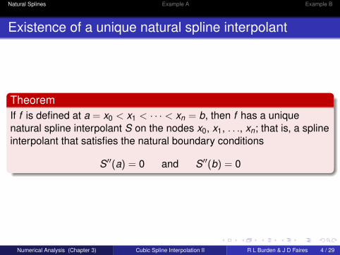
Existence of a unique natural spline interpolant

Theorem

If f is defined at a = x0 < x1 < · · · < xn = b, then f has a unique

natural spline interpolant S on the nodes x0, x1, . . ., xn; that is, a spline

interpolant that satisfies the natural boundary conditions

S′′(a) = 0 and S

′′(b) = 0




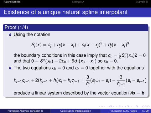
Proof (1/4)

Using the notation

Sj(x) = aj + bj(x − xj) + cj(x − xj)2 + dj(x − xj)

3

the boundary conditions in this case imply that cn = 12S′′

n(xn)2 = 0

and that 0 = S′′(x0) = 2c0 + 6d0(x0 − x0) so c0 = 0.

The two equations c0 = 0 and cn = 0 together with the equations

hj−1cj−1 + 2(hj−1 + hj)cj + hjcj+1 =3

hj(aj+1 − aj)−

3

hj−1(aj − aj−1)

produce a linear system described by the vector equation Ax = b:




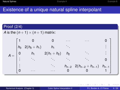
Proof (2/4)

A is the (n + 1) × (n + 1) matrix:

A =

1 0 0 · · · · · · 0

h0 2(h0 + h1) h1. . .

...

0 h1 2(h1 + h2) h2. . .

......

. . .. . .

. . .. . . 0

.... . . hn−2 2(hn−2 + hn−1) hn−1

0 · · · · · · 0 0 1




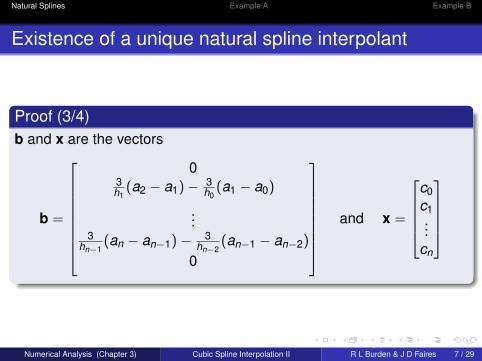
Proof (3/4)

b and x are the vectors

b =

03h1

(a2 − a1) −3h0

(a1 − a0)

...3

hn−1(an − an−1) −

3hn−2

(an−1 − an−2)

0

and x =

c0

c1...

cn



Proof (4/4)

The matrix A is strictly diagonally dominant, that is, in each row

the magnitude of the diagonal entry exceeds the sum of the

magnitudes of all the other entries in the row.


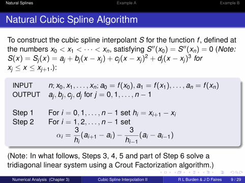
Natural Cubic Spline Algorithm

To construct the cubic spline interpolant S for the function f , defined at

the numbers x0 < x1 < · · · < xn, satisfying S′′(x0) = S′′(xn) = 0 (Note:

S(x) = Sj(x) = aj + bj(x − xj) + cj(x − xj)2 + dj(x − xj)

3 for

xj ≤ x ≤ xj+1.):

INPUT n; x0, x1, . . . , xn; a0 = f (x0), a1 = f (x1), . . . , an = f (xn)OUTPUT aj , bj , cj , dj for j = 0, 1, . . . , n − 1

Step 1 For i = 0, 1, . . . , n − 1 set hi = xi+1 − xi

Step 2 For i = 1, 2, . . . , n − 1 set

αi =3

hi(ai+1 − ai) −

3

hi−1(ai − ai−1)

(Note: In what follows, Steps 3, 4, 5 and part of Step 6 solve a

tridiagonal linear system using a Crout Factorization algorithm.)



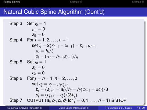
Natural Cubic Spline Algorithm (Cont’d)

Step 3 Set l0 = 1

µ0 = 0

z0 = 0

Step 4 For i = 1, 2, . . . , n − 1

set li = 2(xi+1 − xi−1) − hi−1µi−1

µi = hi/lizi = (αi − hi−1zi−1)/li

Step 5 Set ln = 1

zn = 0

cn = 0

Step 6 For j = n − 1, n − 2, . . . , 0

set cj = zj − µjcj+1

bj = (aj+1 − aj)/hj − hj(cj+1 + 2cj)/3

dj = (cj+1 − cj)/(3hj)Step 7 OUTPUT (aj , bj , cj , dj for j = 0, 1, . . . , n − 1) & STOP



Outline




0ex dx



Natural Spline Interpolant

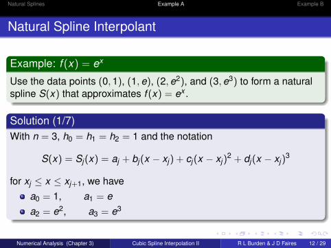
Example: f (x) = ex

Use the data points (0, 1), (1, e), (2, e2), and (3, e3) to form a natural

spline S(x) that approximates f (x) = ex .

Solution (1/7)

With n = 3, h0 = h1 = h2 = 1 and the notation

S(x) = Sj(x) = aj + bj(x − xj) + cj(x − xj)2 + dj(x − xj)

3

for xj ≤ x ≤ xj+1, we have

a0 = 1, a1 = e

a2 = e2, a3 = e3




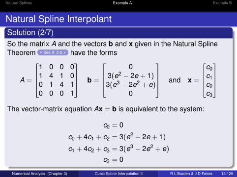
Solution (2/7)

So the matrix A and the vectors b and x given in the Natural Spline

Theorem See A, b & x have the forms

A =

1 0 0 0

1 4 1 0

0 1 4 1

0 0 0 1

b =

0

3(e2− 2e + 1)

3(e3− 2e2 + e)

0

and x =

c0

c1

c2

c3

The vector-matrix equation Ax = b is equivalent to the system:

c0 = 0

c0 + 4c1 + c2 = 3(e2− 2e + 1)

c1 + 4c2 + c3 = 3(e3− 2e

2 + e)

c3 = 0




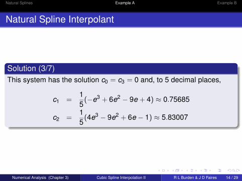
Solution (3/7)

This system has the solution c0 = c3 = 0 and, to 5 decimal places,

c1 =1

5(−e

3 + 6e2− 9e + 4) ≈ 0.75685

c2 =1

5(4e

3− 9e

2 + 6e − 1) ≈ 5.83007




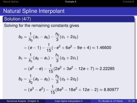
Solution (4/7)

Solving for the remaining constants gives

b0 =1

h0(a1 − a0) −

h0

3(c1 + 2c0)

= (e − 1) −1

15(−e

3 + 6e2− 9e + 4) ≈ 1.46600

b1 =1

h1(a2 − a1) −

h1

3(c2 + 2c1)

= (e2− e) −

1

15(2e

3 + 3e2− 12e + 7) ≈ 2.22285

b2 =1

h2(a3 − a2) −

h2

3(c3 + 2c2)

= (e3− e

2) −1

15(8e

3− 18e

2 + 12e − 2) ≈ 8.80977




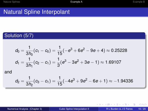
Solution (5/7)

d0 =1

3h0(c1 − c0) =

1

15(−e

3 + 6e2− 9e + 4) ≈ 0.25228

d1 =1

3h1(c2 − c1) =

1

3(e3

− 3e2 + 3e − 1) ≈ 1.69107

and

d2 =1

3h2(c3 − c1) =

1

15(−4e

3 + 9e2− 6e + 1) ≈ −1.94336




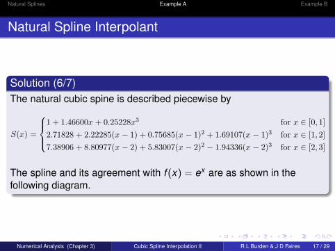
Solution (6/7)

The natural cubic spine is described piecewise by

S(x) =

1 + 1.46600x + 0.25228x3 for x ∈ [0, 1]

2.71828 + 2.22285(x − 1) + 0.75685(x − 1)2 + 1.69107(x − 1)3 for x ∈ [1, 2]

7.38906 + 8.80977(x − 2) + 5.83007(x − 2)2 − 1.94336(x − 2)3 for x ∈ [2, 3]

The spline and its agreement with f (x) = ex are as shown in the

following diagram.




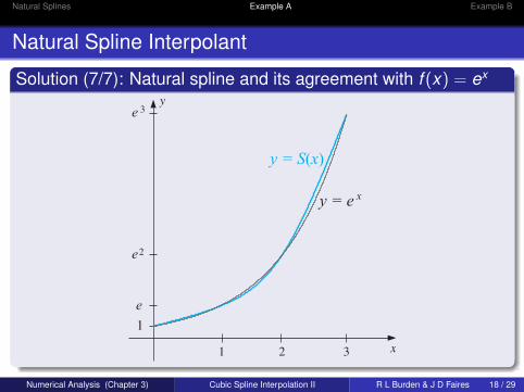
Solution (7/7): Natural spline and its agreement with f (x) = ex

x

y

1

1 2 3

e

e

e

3

2

y = S(x)

y = e x



Outline




0ex dx




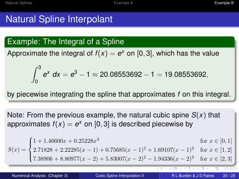
Example: The Integral of a Spline

Approximate the integral of f (x) = ex on [0, 3], which has the value

∫ 3

0

ex

dx = e3− 1 ≈ 20.08553692 − 1 = 19.08553692,

by piecewise integrating the spline that approximates f on this integral.

Note: From the previous example, the natural cubic spine S(x) that

approximates f (x) = ex on [0, 3] is described piecewise by

S(x) =

1 + 1.46600x + 0.25228x3 for x ∈ [0, 1]

2.71828 + 2.22285(x − 1) + 0.75685(x − 1)2 + 1.69107(x − 1)3 for x ∈ [1, 2]

7.38906 + 8.80977(x − 2) + 5.83007(x − 2)2 − 1.94336(x − 2)3 for x ∈ [2, 3]




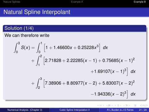
Solution (1/4)

We can therefore write

∫ 3

0

S(x) =

∫ 1

0

[

1 + 1.46600x + 0.25228x3]

dx

+

∫ 2

1

[

2.71828 + 2.22285(x − 1) + 0.75685(x − 1)2

+1.69107(x − 1)3]

dx

+

∫ 3

2

[

7.38906 + 8.80977(x − 2) + 5.83007(x − 2)2

−1.94336(x − 2)3]

dx




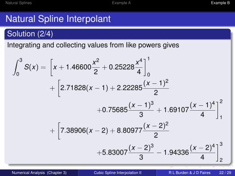
Solution (2/4)

Integrating and collecting values from like powers gives

∫ 3

0

S(x) =

[

x + 1.46600x2

2+ 0.25228

x4

4

]1

0

+

[

2.71828(x − 1) + 2.22285(x − 1)2

2

+0.75685(x − 1)3

3+ 1.69107

(x − 1)4

4

]2

1

+

[

7.38906(x − 2) + 8.80977(x − 2)2

2

+5.83007(x − 2)3

3− 1.94336

(x − 2)4

4

]3

2




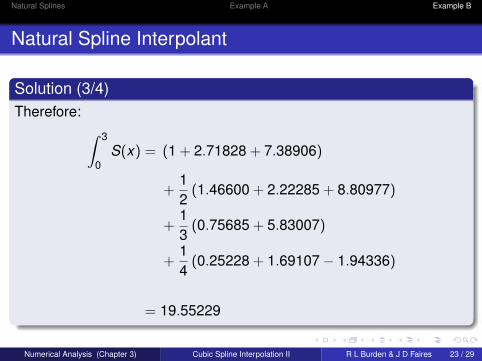
Solution (3/4)

Therefore:

∫ 3

0

S(x) = (1 + 2.71828 + 7.38906)

+1

2(1.46600 + 2.22285 + 8.80977)

+1

3(0.75685 + 5.83007)

+1

4(0.25228 + 1.69107 − 1.94336)

= 19.55229




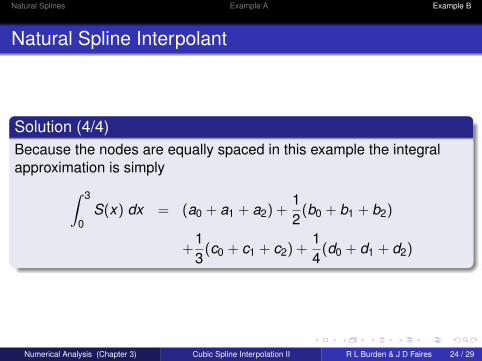
Solution (4/4)

Because the nodes are equally spaced in this example the integral

approximation is simply

∫ 3

0

S(x) dx = (a0 + a1 + a2) +1

2(b0 + b1 + b2)

+1

3(c0 + c1 + c2) +

1

4(d0 + d1 + d2)


Questions?

Reference Material

Cubic Spline Interpolant

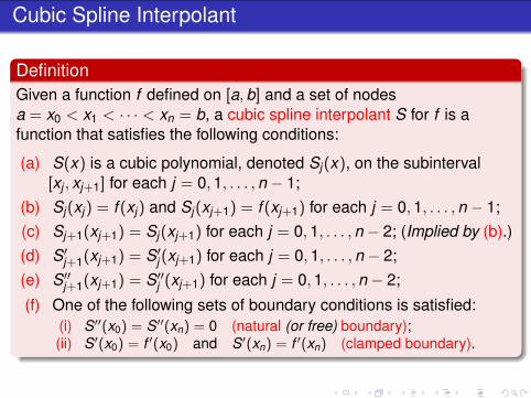
Definition

Given a function f defined on [a, b] and a set of nodes

a = x0 < x1 < · · · < xn = b, a cubic spline interpolant S for f is a

function that satisfies the following conditions:

(a) S(x) is a cubic polynomial, denoted Sj(x), on the subinterval

[xj , xj+1] for each j = 0, 1, . . . , n − 1;

(b) Sj(xj) = f (xj) and Sj(xj+1) = f (xj+1) for each j = 0, 1, . . . , n − 1;

(c) Sj+1(xj+1) = Sj(xj+1) for each j = 0, 1, . . . , n − 2; (Implied by (b).)

(d) S′

j+1(xj+1) = S′

j (xj+1) for each j = 0, 1, . . . , n − 2;

(e) S′′

j+1(xj+1) = S′′

j (xj+1) for each j = 0, 1, . . . , n − 2;

(f) One of the following sets of boundary conditions is satisfied:

(i) S′′(x0) = S′′(xn) = 0 (natural (or free) boundary);

(ii) S′(x0) = f ′(x0) and S′(xn) = f ′(xn) (clamped boundary).

Strictly Diagonally Dominant Matrices

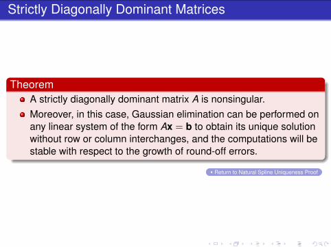
Theorem

A strictly diagonally dominant matrix A is nonsingular.

Moreover, in this case, Gaussian elimination can be performed on

any linear system of the form Ax = b to obtain its unique solution

without row or column interchanges, and the computations will be

stable with respect to the growth of round-off errors.

Return to Natural Spline Uniqueness Proof

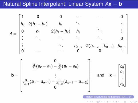
Natural Spline Interpolant: Linear System Ax = b

A =

1 0 0 · · · · · · 0

h0 2(h0 + h1) h1. . .

...

0 h1 2(h1 + h2) h2. . .

......

. . .. . .

. . .. . . 0

.... . . hn−2 2(hn−2 + hn−1) hn−1

0 · · · · · · 0 0 1

b =

03h1

(a2 − a1) −3h0

(a1 − a0)

...3

hn−1(an − an−1) −

3hn−2

(an−1 − an−2)

0

and x =

c0

c1...

cn

Return to Natural Spline Example (f (x) = ex )

Documents

Interpolation & Polynomial Approximation Cubic …...Interpolation & Polynomial Approximation Cubic Spline Interpolation II Numerical Analysis (9th Edition) R L Burden & J D Faires