Embed Size (px)
Citation preview
4/21/2017
1
Energy Systems Research Laboratory, FIU
Internal Rate of Return
• We consider a cash-flow set
• The value of d for which
is called the internal rate of return (IRR)
• The IRR is a measure of how fast we recover an investment or stated differently, the speed with which the returns recover an investment
: , 1, 2, ...tA A t 0
nt
tt 0
P A 0
Professor O. A. Mohammed, EEL5285 Lecture Notes, Spring 2017
Energy Systems Research Laboratory, FIU
Internal Rate of Return Example
• Consider the following cash-flow set
Professor O. A. Mohammed, EEL5285 Lecture Notes, Spring 2017
4/21/2017
2
Energy Systems Research Laboratory, FIU
Internal Rate of Return
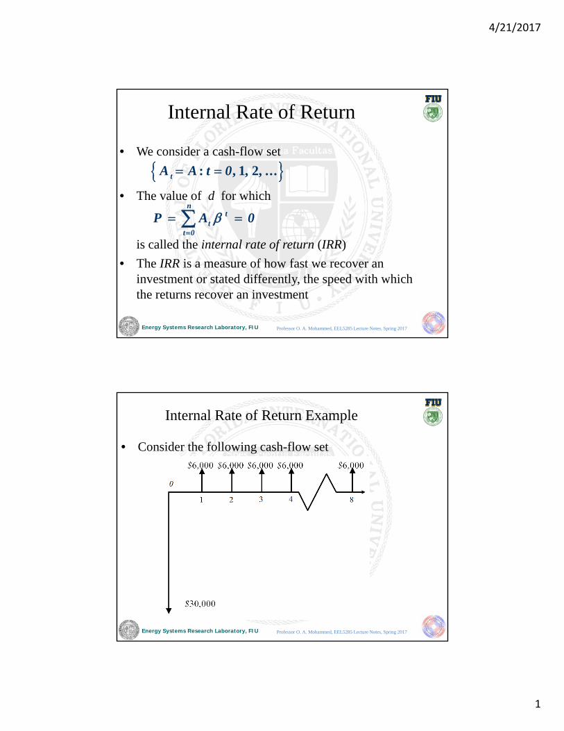
• The present value
has the (non-obvious) solution of d equal to about 12%.
• The interpretation is that under a 12% discount rate, the present value of the cash flow set is 0 and so 12% is the IRR for the given cash- flow set– The investment makes sense as long as other investments yield
less than 12%.
8130,000 6,000P 0
d
1
1 d
Professor O. A. Mohammed, EEL5285 Lecture Notes, Spring 2017
Energy Systems Research Laboratory, FIU
Internal Rate of Return
• Consider an infinite horizon simple investment
• Therefore
• For I = $ 1,000 and A = $ 200, d = 20% and we interpret that the returns capture 20% of the investment each year or equivalently that we have a simple payback period of 5 years
IA
dI
ratio of annual return to initial investment
A A A
0 1 2
. . .n
Professor O. A. Mohammed, EEL5285 Lecture Notes, Spring 2017
4/21/2017
3
Energy Systems Research Laboratory, FIU
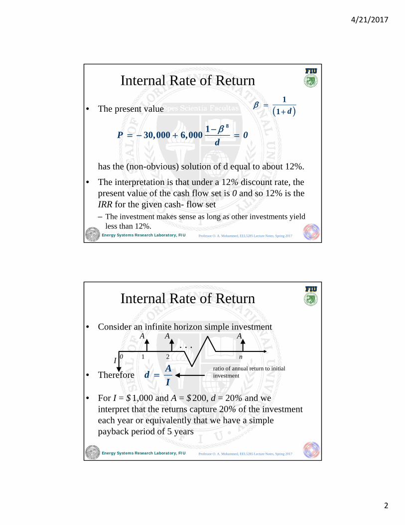
Efficient Refrigerator Example
• A more efficient refrigerator incurs an investment of additional $1,000 but provides $200 of energy savings annually
• For a lifetime of 10 years, the IRR is computed from the solution of
or
1011,000 2000
d
1015
d
The solution of this equation requires either an iterative approach or a value looked up from a table
Professor O. A. Mohammed, EEL5285 Lecture Notes, Spring 2017
Energy Systems Research Laboratory, FIU
Efficient Refrigerator Example, cont.
•IRR tables show that
and so the IRR is approximately 15%
If the refrigerator has an expected lifetime of 15 years this value becomes
10
15
15.02
d %d
15
18.4
15.00
d %d
As was mentioned earlier, the value is 20% if it lasts forever
Professor O. A. Mohammed, EEL5285 Lecture Notes, Spring 2017

4/21/2017
4
Energy Systems Research Laboratory, FIU
NY Times– Cost of Green Power
• Invenergy had a contract to sell power in Virginia – but state regulators rejected the deal, citing the recession, low natural gas prices
• A number of projects are being cancelled or delayed
• In Florida, Idaho, Kentucky, and Virginia deals to buy renewable energy have slowed
• Rhode Island regulators rejected a dealfor 24.4 cent/kWh off-shore wind power
http://www.nytimes.com/2010/11/08/science/earth/08fossil.html?_r=2&hp
Professor O. A. Mohammed, EEL5285 Lecture Notes, Spring 2017
Energy Systems Research Laboratory, FIU
In the news: Renewable Energy Mandate Scrutiny (Example from the State of Wisconsin)
• Target is to supply 10% from renewables by 2015
• Changes are forecast in renewable energy policy, possibly delaying this deadline
• New administration will take a look at the “costs of going green”
• Some expect lawmakers to take up a repeal of Wisconsin's moratorium on construction of nuclear reactors
• Environmental group “Clean Wisconsin” – “A key priority would be making sure we continue to invest aggressively in energy efficiency”
http://www.jsonline.com/business/106807903.html
Professor O. A. Mohammed, EEL5285 Lecture Notes, Spring 2017
4/21/2017
5
Energy Systems Research Laboratory, FIU
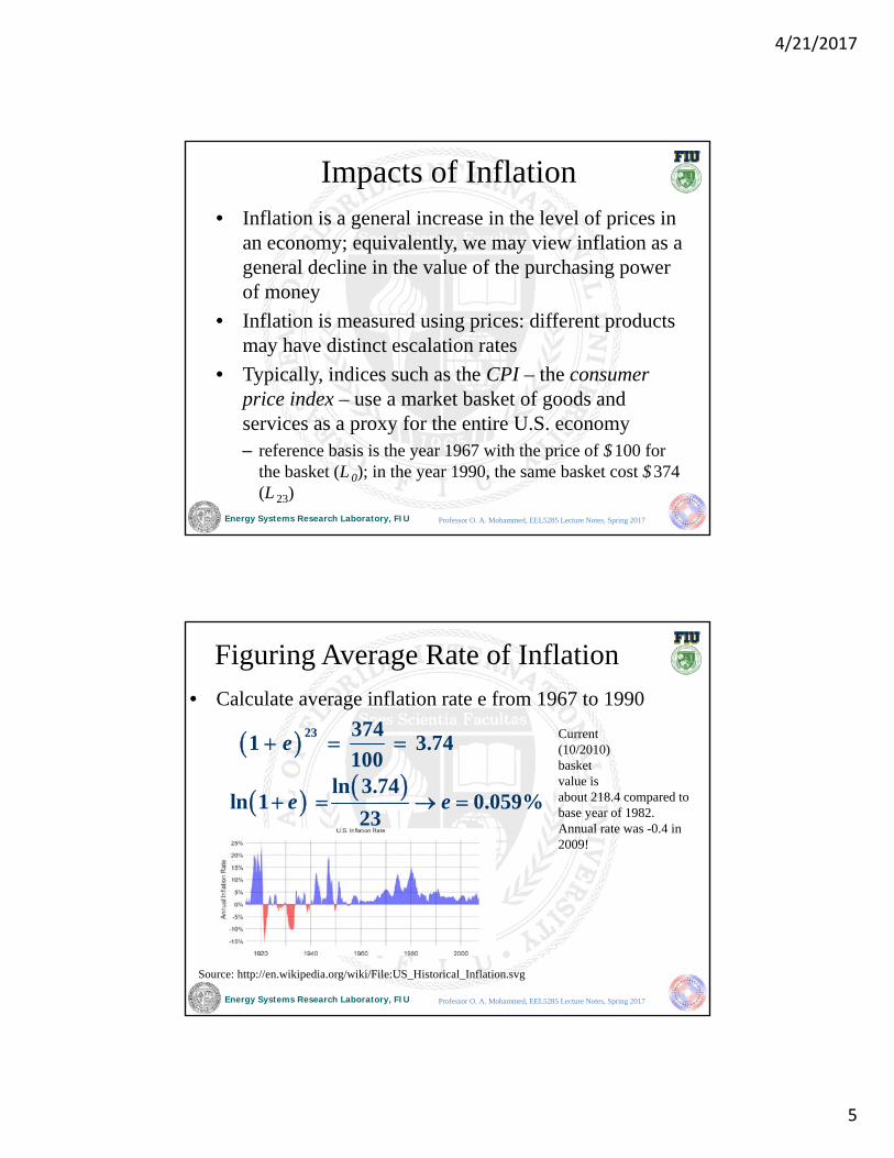
Impacts of Inflation• Inflation is a general increase in the level of prices in
an economy; equivalently, we may view inflation as a general decline in the value of the purchasing power of money
• Inflation is measured using prices: different products may have distinct escalation rates
• Typically, indices such as the CPI – the consumer price index – use a market basket of goods and services as a proxy for the entire U.S. economy– reference basis is the year 1967 with the price of $100 for
the basket (L 0); in the year 1990, the same basket cost $374 (L 23)
Professor O. A. Mohammed, EEL5285 Lecture Notes, Spring 2017
Energy Systems Research Laboratory, FIU
Figuring Average Rate of Inflation
• Calculate average inflation rate e from 1967 to 1990
23 3741 3.74
100e
ln 3.74ln 1 0.059%
23e e
Source: http://en.wikipedia.org/wiki/File:US_Historical_Inflation.svg
Current(10/2010)basketvalue is about 218.4 compared to base year of 1982. Annual rate was -0.4 in 2009!
Professor O. A. Mohammed, EEL5285 Lecture Notes, Spring 2017
4/21/2017
6
Energy Systems Research Laboratory, FIU
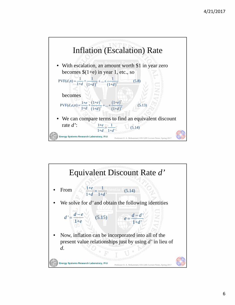
Inflation (Escalation) Rate
• With escalation, an amount worth $1 in year zero becomes $(1+e) in year 1, etc., so
becomes
• We can compare terms to find an equivalent discount rate d’:
2
1 1 1PVF( , ) + ... (5.8)
1+ 1+ 1+nd n
d d d
2
2
1+ 1+1+PVF( , , ) + ... (5.13)
1+ 1+ 1+
n
n
e eed e n
d d d
1+ 1 (5.14)
1+ 1+ '
e
d d
Professor O. A. Mohammed, EEL5285 Lecture Notes, Spring 2017
Energy Systems Research Laboratory, FIU
Equivalent Discount Rate d’
• From
• We solve for d’ and obtain the following identities
• Now, inflation can be incorporated into all of the present value relationships just by using d’ in lieu of d.
1+ 1 (5.14)
1+ 1+ '
e
d d
' (5.15)1+
d ed
e
'
1+ '
d de
d
Professor O. A. Mohammed, EEL5285 Lecture Notes, Spring 2017
4/21/2017
7
Energy Systems Research Laboratory, FIU
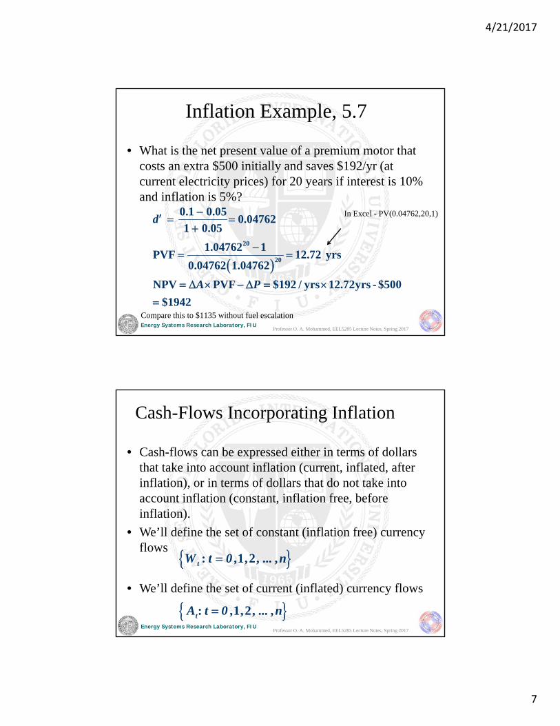
Inflation Example, 5.7
• What is the net present value of a premium motor that costs an extra $500 initially and saves $192/yr (at current electricity prices) for 20 years if interest is 10% and inflation is 5%?
20
20
0.1 0.050.04762
1 0.05
1.04762 1PVF 12.72 yrs
0.04762 1.04762
NPV PVF $192 / yrs 12.72yrs - $500
$1942
d
A P
Compare this to $1135 without fuel escalation
In Excel - PV(0.04762,20,1)
Professor O. A. Mohammed, EEL5285 Lecture Notes, Spring 2017
Energy Systems Research Laboratory, FIU
Cash-Flows Incorporating Inflation
• Cash-flows can be expressed either in terms of dollars that take into account inflation (current, inflated, after inflation), or in terms of dollars that do not take into account inflation (constant, inflation free, before inflation).
• We’ll define the set of constant (inflation free) currency flows
• We’ll define the set of current (inflated) currency flows
: 1,2, ... ,tA t 0 , n
: ,1,2, ... ,tW t 0 n
Professor O. A. Mohammed, EEL5285 Lecture Notes, Spring 2017
4/21/2017
8
Energy Systems Research Laboratory, FIU
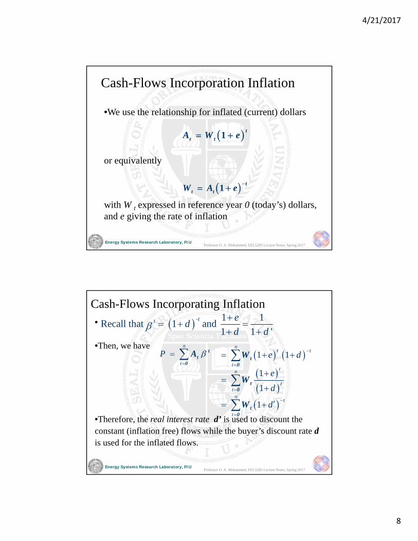
Cash-Flows Incorporation Inflation
•We use the relationship for inflated (current) dollars
or equivalently
with W t expressed in reference year 0 (today’s) dollars, and e giving the rate of inflation
1t
t tA W e
1t
t tW A e
Professor O. A. Mohammed, EEL5285 Lecture Notes, Spring 2017
Energy Systems Research Laboratory, FIU
Cash-Flows Incorporating Inflation
•
•Then, we have
•Therefore, the real interest rate d’ is used to discount the constant (inflation free) flows while the buyer’s discount rate dis used for the inflated flows.
n
t
P
tt
0
A
1 1
1
1
1
nt t
ttn
tt
nt
t
e d
e
d
d
t0
t0
t0
W
W
W
- 1 1Recall that 1 and
1 1 'tt e
dd d
Professor O. A. Mohammed, EEL5285 Lecture Notes, Spring 2017
4/21/2017
9
Energy Systems Research Laboratory, FIU
Cash-Flows Incorporating Inflation
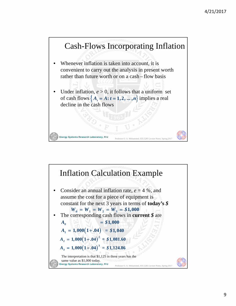
• Whenever inflation is taken into account, it is convenient to carry out the analysis in present worth rather than future worth or on a cash – flow basis
• Under inflation, e > 0, it follows that a uniform set of cash flows implies a real decline in the cash flows
: 1,2, ... ,tA A t n
Professor O. A. Mohammed, EEL5285 Lecture Notes, Spring 2017
Energy Systems Research Laboratory, FIU
Inflation Calculation Example
• Consider an annual inflation rate, e = 4 %, and assume the cost for a piece of equipment is constant for the next 3 years in terms of today’s $
• The corresponding cash flows in current $ are
1
1,000
1,000 1 .04 1,040
0A $
A = $
1 2 3 1,0000W W W W $
2
2
3
3
1,000 1 .04 1,081.60
1,000 1 .04 1,124.86
A = $
A = $
The interpretation is that $1,125 in three years has the same value as $1,000 today.
Professor O. A. Mohammed, EEL5285 Lecture Notes, Spring 2017
4/21/2017
10
Energy Systems Research Laboratory, FIU
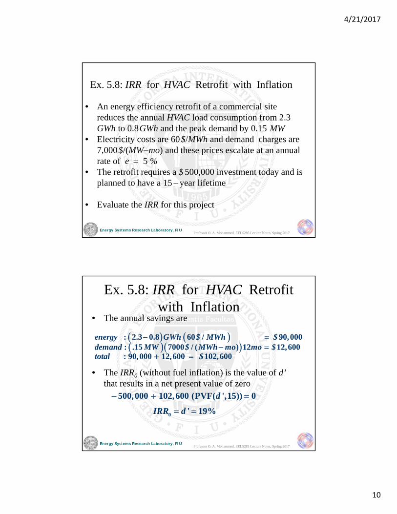
Ex. 5.8: IRR for HVAC Retrofit with Inflation
• An energy efficiency retrofit of a commercial site reduces the annual HVAC load consumption from 2.3 GWh to 0.8GWh and the peak demand by 0.15 MW
• Electricity costs are 60$/MWh and demand charges are 7,000$/(MWmo) and these prices escalate at an annual rate of e 5 %
• The retrofit requires a $ 500,000 investment today and is planned to have a 15 – year lifetime
• Evaluate the IRR for this project
Professor O. A. Mohammed, EEL5285 Lecture Notes, Spring 2017
Energy Systems Research Laboratory, FIU
Ex. 5.8: IRR for HVAC Retrofit with Inflation
• The annual savings are
• The IRR0 (without fuel inflation) is the value of d’that results in a net present value of zero
: 2.3 0.8 60 / 90,000: .15 7000 / ( ) 12 12,600: 90,000 12,600 102,600
energy GWh $ MWh $demand MW $ MWh mo mo $total $
500,000 102,600 (PVF( ',15)) 0d
0 ' 19%IRR d
Professor O. A. Mohammed, EEL5285 Lecture Notes, Spring 2017
4/21/2017
11
Energy Systems Research Laboratory, FIU
Ex. 5.8: IRR for HVAC Retrofit with Inflation
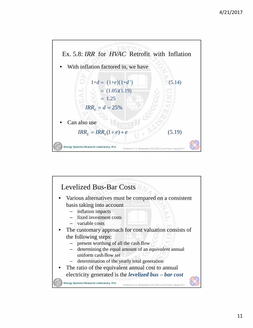
• With inflation factored in, we have
• Can also use
1+ 1+ 1+ ' (5.14)
(1.05)(1.19)
1.25
d e d
25%EIRR d
0 (1 ) (5.19)EIRR IRR e e
Professor O. A. Mohammed, EEL5285 Lecture Notes, Spring 2017
Energy Systems Research Laboratory, FIU
Levelized Bus-Bar Costs
• Various alternatives must be compared on a consistent basis taking into account
– inflation impacts– fixed investment costs– variable costs
• The customary approach for cost valuation consists of the following steps:
– present worthing of all the cash-flow – determining the equal amount of an equivalent annual
uniform cash-flow set– determination of the yearly total generation
• The ratio of the equivalent annual cost to annual electricity generated is the levelized bus – bar cost
Professor O. A. Mohammed, EEL5285 Lecture Notes, Spring 2017
4/21/2017
12
Energy Systems Research Laboratory, FIU
Levelized Bus-Bar Costs
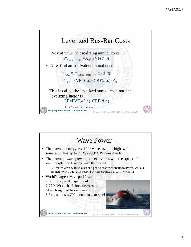
• Present value of escalating annual costs
• Now find an equivalent annual cost
This is called the levelized annual cost, and the levelizing factor is
annual costs 0PV =A PVF( ', )d n
A,L annual costsC =PV CRF( , )d n
LF=PVF( ', ) CRF( , )d n d n
A,L 0C =PVF( ', ) CRF( , ) Ad n d n
LF = 1 means no inflation
Professor O. A. Mohammed, EEL5285 Lecture Notes, Spring 2017
Energy Systems Research Laboratory, FIU
Wave Power• The potential energy available waves is quite high, with
some estimates up to 2 TW (2000 GW) worldwide.
• The potential wave power per meter varies with the square of the wave height and linearly with the period. – A 3 meter wave with an 8 second period produces about 36 kW/m, while a
15 meter wave with a 15 second period produces about 1.7 MW/m.
• World’s largest wave park” was in Portugal, with capacity of 2.25 MW; each of three devices is142m long, and has a diameter of 3.5 m, and uses 700 metric tons of steel
Professor O. A. Mohammed, EEL5285 Lecture Notes, Spring 2017
4/21/2017
13
Energy Systems Research Laboratory, FIU
Wave Power, Recent News
• The 9 million Euro Agucadoura project was taken off-line indefinitely in Nov 2008 because of leaks; once leaks were fixed they couldn’t get financing to restart.
• On Nov 2, 2010 Pacific Gas and Electric suspended its WaveConnect Project, which was to have used buoys to generate power in Pacific off of the Humboldt County, CA coast saying that the cost of getting government permits, installing the devices and the associated infrastructure make the project untenable.
• For years wave power has appeared to be “right around the corner” but turning the corner is quite difficult. Still there is still ongoing work.
Professor O. A. Mohammed, EEL5285 Lecture Notes, Spring 2017
Energy Systems Research Laboratory, FIU
Wave Power
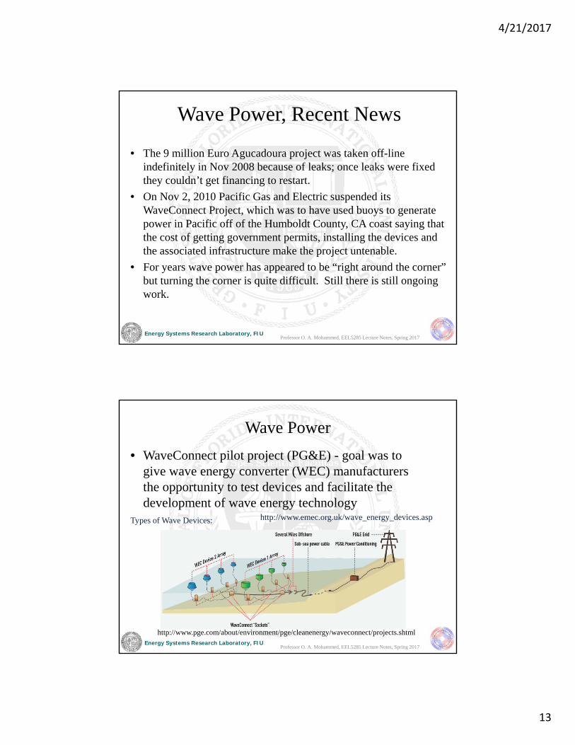
• WaveConnect pilot project (PG&E) - goal was to give wave energy converter (WEC) manufacturers the opportunity to test devices and facilitate the development of wave energy technology
http://www.pge.com/about/environment/pge/cleanenergy/waveconnect/projects.shtml
http://www.emec.org.uk/wave_energy_devices.aspTypes of Wave Devices:
Professor O. A. Mohammed, EEL5285 Lecture Notes, Spring 2017
4/21/2017
14
Energy Systems Research Laboratory, FIU
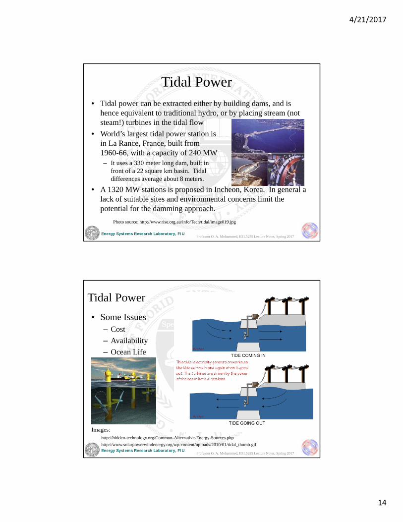
Tidal Power• Tidal power can be extracted either by building dams, and is
hence equivalent to traditional hydro, or by placing stream (not steam!) turbines in the tidal flow
• World’s largest tidal power station is in La Rance, France, built from 1960-66, with a capacity of 240 MW– It uses a 330 meter long dam, built in
front of a 22 square km basin. Tidal differences average about 8 meters.
• A 1320 MW stations is proposed in Incheon, Korea. In general a lack of suitable sites and environmental concerns limit the potential for the damming approach.
Photo source: http://www.rise.org.au/info/Tech/tidal/image019.jpg
Professor O. A. Mohammed, EEL5285 Lecture Notes, Spring 2017
Energy Systems Research Laboratory, FIU
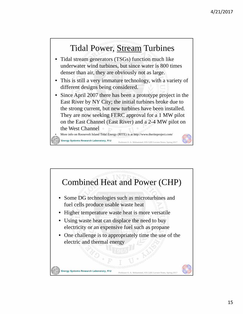
Tidal Power
• Some Issues– Cost
– Availability
– Ocean Life
http://www.solarpowerwindenergy.org/wp-content/uploads/2010/01/tidal_thumb.gif
http://hidden-technology.org/Common-Alternative-Energy-Sources.php
Images:
Professor O. A. Mohammed, EEL5285 Lecture Notes, Spring 2017
4/21/2017
15
Energy Systems Research Laboratory, FIU
Tidal Power, Stream Turbines• Tidal stream generators (TSGs) function much like
underwater wind turbines, but since water is 800 times denser than air, they are obviously not as large.
• This is still a very immature technology, with a variety of different designs being considered.
• Since April 2007 there has been a prototype project in the East River by NY City; the initial turbines broke due to the strong current, but new turbines have been installed. They are now seeking FERC approval for a 1 MW pilot on the East Channel (East River) and a 2-4 MW pilot on the West Channel
• More info on Roosevelt Island Tidal Energy (RITE) is at http://www.theriteproject.com/
Professor O. A. Mohammed, EEL5285 Lecture Notes, Spring 2017
Energy Systems Research Laboratory, FIU
Combined Heat and Power (CHP)
• Some DG technologies such as microturbines and fuel cells produce usable waste heat
• Higher temperature waste heat is more versatile
• Using waste heat can displace the need to buy electricity or an expensive fuel such as propane
• One challenge is to appropriately time the use of the electric and thermal energy
Professor O. A. Mohammed, EEL5285 Lecture Notes, Spring 2017

4/21/2017
16
Energy Systems Research Laboratory, FIU
CHP Regional Application Centers• Project sponsored by US Department of Energy
• Goal is to double the amount of installed CHP capacity (from 1988) for 46,000 MW of new capacity
• Include internal combustion engines, microturbines, and fuel cells
• Recovered thermal energy used for cooling, heating, controlling humidity
http://www.chpcentermw.org/home.html
Professor O. A. Mohammed, EEL5285 Lecture Notes, Spring 2017
Energy Systems Research Laboratory, FIU
Current Status
Source: EIA 2010 Electric Power Annual http://www.eia.doe.gov/cneaf/electricity/epa/epa.pdf
2008 and 2009 continued downward trend, 1.617 quad and 1.552 respectively; for electric it is 0.292 and 0.286.
Professor O. A. Mohammed, EEL5285 Lecture Notes, Spring 2017
4/21/2017
17
Energy Systems Research Laboratory, FIU
CHP Efficiency – Simple approach
• Difficult to quantify – the value of a unit of electricity is much higher than unit of thermal energy
• Simplest approach:
• Doesn’t distinguish between the two types of energy
Overall Thermal Electrical Output + Thermal Outputx100% (5.29)
Efficiency Thermal Input
Professor O. A. Mohammed, EEL5285 Lecture Notes, Spring 2017
Energy Systems Research Laboratory, FIU
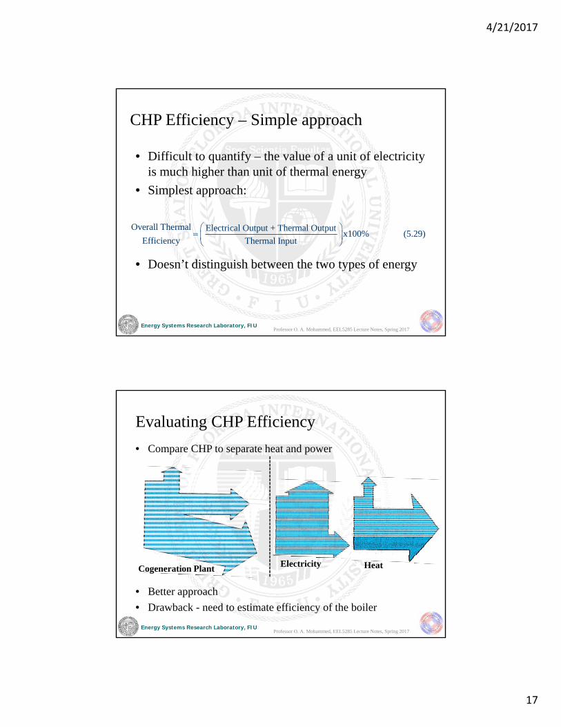
Evaluating CHP Efficiency
• Compare CHP to separate heat and power
• Better approach
• Drawback - need to estimate efficiency of the boiler
Cogeneration Plant Electricity Heat
Professor O. A. Mohammed, EEL5285 Lecture Notes, Spring 2017
4/21/2017
18
Energy Systems Research Laboratory, FIU
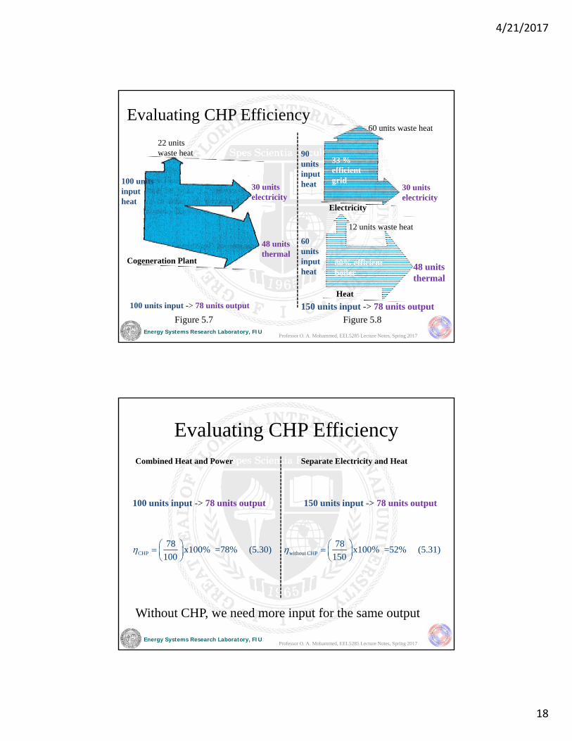
Evaluating CHP Efficiency
Cogeneration Plant
Electricity
Heat
Figure 5.7 Figure 5.8
100 units inputheat
22 units waste heat
60 units waste heat
12 units waste heat
90 units inputheat
60 units inputheat 48 units
thermal
30 units electricity
30 units electricity
48 units thermal
100 units input -> 78 units output 150 units input -> 78 units output
33 % efficient grid
80% efficient boiler
Professor O. A. Mohammed, EEL5285 Lecture Notes, Spring 2017
Energy Systems Research Laboratory, FIU
Evaluating CHP Efficiency
Without CHP, we need more input for the same output
Combined Heat and Power
100 units input -> 78 units output
Separate Electricity and Heat
150 units input -> 78 units output
CHP
78x100% =78% (5.30)
100
without CHP
78x100% =52% (5.31)
150
Professor O. A. Mohammed, EEL5285 Lecture Notes, Spring 2017
4/21/2017
19
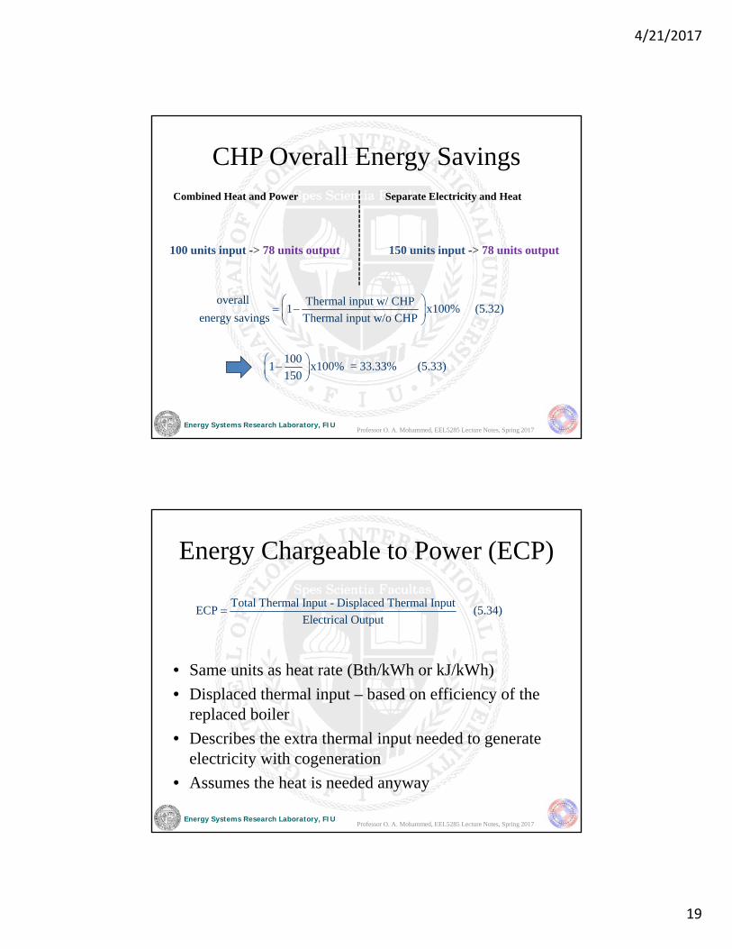
Energy Systems Research Laboratory, FIU
CHP Overall Energy Savings
overall Thermal input w/ CHP1 x100% (5.32)
energy savings Thermal input w/o CHP
Combined Heat and Power Separate Electricity and Heat
1001 x100% = 33.33% (5.33)
150
100 units input -> 78 units output 150 units input -> 78 units output
Professor O. A. Mohammed, EEL5285 Lecture Notes, Spring 2017
Energy Systems Research Laboratory, FIU
Energy Chargeable to Power (ECP)
• Same units as heat rate (Bth/kWh or kJ/kWh)
• Displaced thermal input – based on efficiency of the replaced boiler
• Describes the extra thermal input needed to generate electricity with cogeneration
• Assumes the heat is needed anyway
Total Thermal Input - Displaced Thermal InputECP (5.34)
Electrical Output
Professor O. A. Mohammed, EEL5285 Lecture Notes, Spring 2017
4/21/2017
20
Energy Systems Research Laboratory, FIU
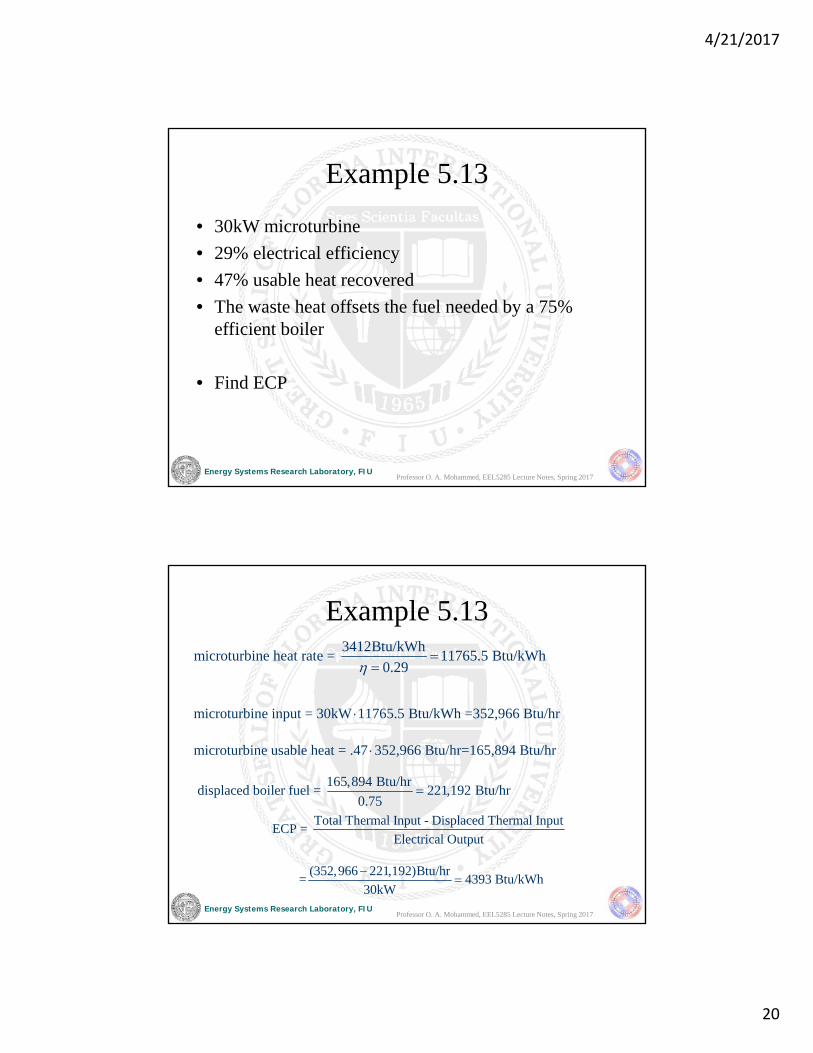
Example 5.13
• 30kW microturbine
• 29% electrical efficiency
• 47% usable heat recovered
• The waste heat offsets the fuel needed by a 75% efficient boiler
• Find ECP
Professor O. A. Mohammed, EEL5285 Lecture Notes, Spring 2017
Energy Systems Research Laboratory, FIU
Example 5.133412Btu/kWh
microturbine heat rate = 11765.5 Btu/kWh0.29
microturbine input = 30kW 11765.5 Btu/kWh =352,966 Btu/hr
microturbine usable heat = .47 352,966 Btu/hr=165,894 Btu/hr
165,894 Btu/hrdisplaced boiler fuel = 221,192 Btu/hr
0.75
Total Thermal Input - Displaced Thermal InputECP =
Electrical Output
(352,966 221,192)Btu/hr = 4393 Btu/kWh
30kW
Professor O. A. Mohammed, EEL5285 Lecture Notes, Spring 2017
4/21/2017
21
Energy Systems Research Laboratory, FIU
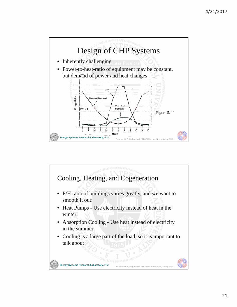
Design of CHP Systems• Inherently challenging
• Power-to-heat-ratio of equipment may be constant, but demand of power and heat changes
Figure 5. 11
Professor O. A. Mohammed, EEL5285 Lecture Notes, Spring 2017
Energy Systems Research Laboratory, FIU
Cooling, Heating, and Cogeneration
• P/H ratio of buildings varies greatly, and we want to smooth it out:
• Heat Pumps - Use electricity instead of heat in the winter
• Absorption Cooling - Use heat instead of electricity in the summer
• Cooling is a large part of the load, so it is important to talk about
Professor O. A. Mohammed, EEL5285 Lecture Notes, Spring 2017
4/21/2017
22
Energy Systems Research Laboratory, FIU
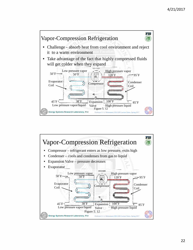
Figure 5. 12
Compressor
Expansion Valve
85˚F
95˚F120˚F
100˚F38˚F45˚F
50˚F
Evaporator Coil
Condenser Coil
50˚F
Vapor-Compression Refrigeration
• Challenge - absorb heat from cool environment and reject it to a warm environment
• Take advantage of the fact that highly compressed fluids will get colder when they expand
High pressure liquidLow pressure vapor/liquid
Low pressure vapor High pressure vapor
Professor O. A. Mohammed, EEL5285 Lecture Notes, Spring 2017
Energy Systems Research Laboratory, FIU
Vapor-Compression Refrigeration• Compressor – refrigerant enters as low pressure, exits high
• Condenser – cools and condenses from gas to liquid
• Expansion Valve – pressure decreases
• Evaporator
Figure 5. 12
Compressor
Expansion Valve
85˚F
95˚F120˚F
100˚F38˚F45˚F
50˚F
Evaporator Coil
Condenser Coil
50˚F
High pressure liquidLow pressure vapor/liquid
Low pressure vapor High pressure vapor
Professor O. A. Mohammed, EEL5285 Lecture Notes, Spring 2017
4/21/2017
23
Energy Systems Research Laboratory, FIU
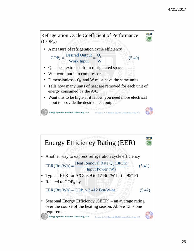
Refrigeration Cycle Coefficient of Performance (COPR)
• A measure of refrigeration cycle efficiency
• QL = heat extracted from refrigerated space
• W = work put into compressor
• Dimensionless - QL and W must have the same units
• Tells how many units of heat are removed for each unit of energy consumed by the A/C
• Want this to be high- if it is low, you need more electrical input to provide the desired heat output
LR
QDesired OutputCOP (5.40)
Work Input W
Professor O. A. Mohammed, EEL5285 Lecture Notes, Spring 2017
Energy Systems Research Laboratory, FIU
Energy Efficiency Rating (EER)
• Another way to express refrigeration cycle efficiency
• Typical EER for A/Cs is 9 to 17 Btu/W-hr (at 95 F)
• Related to COPR by
• Seasonal Energy Efficiency (SEER) – an average rating over the course of the heating season. Above 13 is one requirement
LHeat Removal Rate Q (Btu/h)EER(Btu/Wh) (5.41)
Input Power (W)
REER(Btu/Wh) COP 3.412 Btu/W-hr (5.42)
Professor O. A. Mohammed, EEL5285 Lecture Notes, Spring 2017

4/21/2017
24
Energy Systems Research Laboratory, FIU
One “ton” of cooling
• The rate heat is absorbed when a 1 ton block of ice melts
• Another efficiency measure – tons/kW of cooling:
• A 3-ton home-sized A/C uses approximately 2-3kW
• Chillers can make ice at night to melt during the day
2000 lb 144 Btu/lb1 ton of cooling = =12,000 Btu/h (5.43)
24 h
12,000 Btu/h-ton 12kW/ton = = (5.43)
EER (Btu/Wh) 1000 W/kW EER
Professor O. A. Mohammed, EEL5285 Lecture Notes, Spring 2017
Energy Systems Research Laboratory, FIU
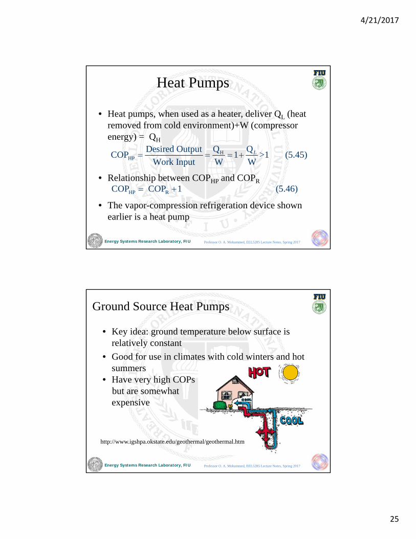
Heat Pumps
• Move heat from a source to sink
• Have the ability to be reversed – provide heating and cooling
Figure 5. 15
Professor O. A. Mohammed, EEL5285 Lecture Notes, Spring 2017
4/21/2017
25
Energy Systems Research Laboratory, FIU
Heat Pumps
• Heat pumps, when used as a heater, deliver QL (heat removed from cold environment)+W (compressor energy) = QH
• Relationship between COPHP and COPR
• The vapor-compression refrigeration device shown earlier is a heat pump
HHP
Q QDesired OutputCOP 1 >1 (5.45)
Work Input W WL
HP RCOP COP 1 (5.46)
Professor O. A. Mohammed, EEL5285 Lecture Notes, Spring 2017
Energy Systems Research Laboratory, FIU
Ground Source Heat Pumps
• Key idea: ground temperature below surface is relatively constant
• Good for use in climates with cold winters and hot summers
• Have very high COPsbut are somewhat expensive
http://www.igshpa.okstate.edu/geothermal/geothermal.htm
Professor O. A. Mohammed, EEL5285 Lecture Notes, Spring 2017
4/21/2017
26
Energy Systems Research Laboratory, FIU
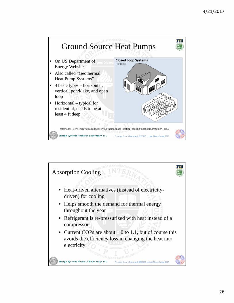
Ground Source Heat Pumps
• On US Department of Energy Website
• Also called “Geothermal Heat Pump Systems”
• 4 basic types – horizontal, vertical, pond/lake, and open loop
• Horizontal – typical for residential, needs to be at least 4 ft deep
http://apps1.eere.energy.gov/consumer/your_home/space_heating_cooling/index.cfm/mytopic=12650
Professor O. A. Mohammed, EEL5285 Lecture Notes, Spring 2017
Energy Systems Research Laboratory, FIU
Absorption Cooling
• Heat-driven alternatives (instead of electricity-driven) for cooling
• Helps smooth the demand for thermal energy throughout the year
• Refrigerant is re-pressurized with heat instead of a compressor
• Current COPs are about 1.0 to 1.1, but of course this avoids the efficiency loss in changing the heat into electricity
Professor O. A. Mohammed, EEL5285 Lecture Notes, Spring 2017
4/21/2017
27
Energy Systems Research Laboratory, FIU
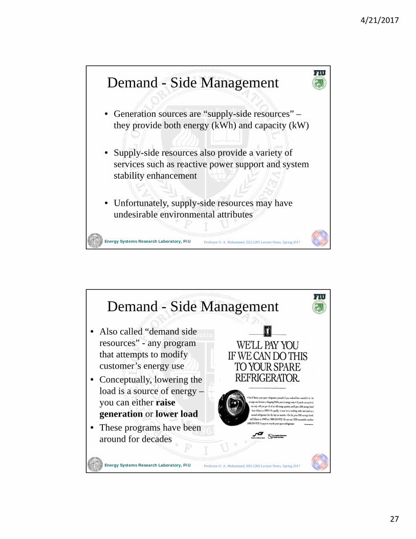
Demand - Side Management
• Generation sources are “supply-side resources” –they provide both energy (kWh) and capacity (kW)
• Supply-side resources also provide a variety of services such as reactive power support and system stability enhancement
• Unfortunately, supply-side resources may have undesirable environmental attributes
Professor O. A. Mohammed, EEL5285 Lecture Notes, Spring 2017
Energy Systems Research Laboratory, FIU
Demand - Side Management
• Also called “demand side resources” - any program that attempts to modify customer’s energy use
• Conceptually, lowering the load is a source of energy –you can either raise generation or lower load
• These programs have beenaround for decades
Professor O. A. Mohammed, EEL5285 Lecture Notes, Spring 2017
4/21/2017
28
Energy Systems Research Laboratory, FIU
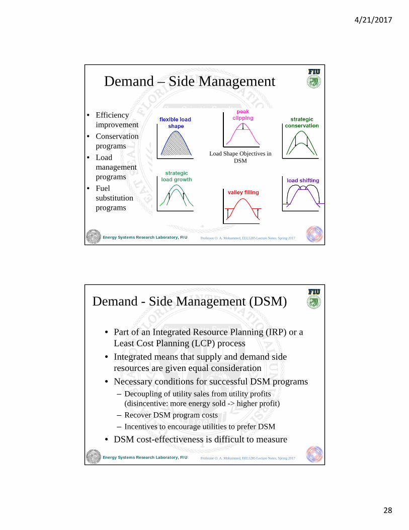
Demand – Side Management
• Efficiency improvement
• Conservation programs
• Load management programs
• Fuel substitution programs
Load Shape Objectives in DSM
Professor O. A. Mohammed, EEL5285 Lecture Notes, Spring 2017
Energy Systems Research Laboratory, FIU
Demand - Side Management (DSM)
• Part of an Integrated Resource Planning (IRP) or a Least Cost Planning (LCP) process
• Integrated means that supply and demand side resources are given equal consideration
• Necessary conditions for successful DSM programs– Decoupling of utility sales from utility profits
(disincentive: more energy sold -> higher profit)
– Recover DSM program costs
– Incentives to encourage utilities to prefer DSM
• DSM cost-effectiveness is difficult to measure
Professor O. A. Mohammed, EEL5285 Lecture Notes, Spring 2017
4/21/2017
29
Energy Systems Research Laboratory, FIU
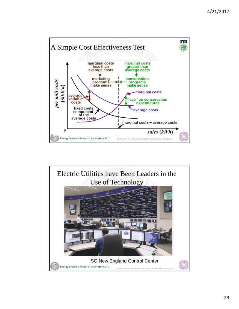
A Simple Cost Effectiveness Test
Professor O. A. Mohammed, EEL5285 Lecture Notes, Spring 2017
Energy Systems Research Laboratory, FIU
Electric Utilities have Been Leaders in the Use of Technology
ISO New England Control Center
Professor O. A. Mohammed, EEL5285 Lecture Notes, Spring 2017
4/21/2017
30
Energy Systems Research Laboratory, FIU
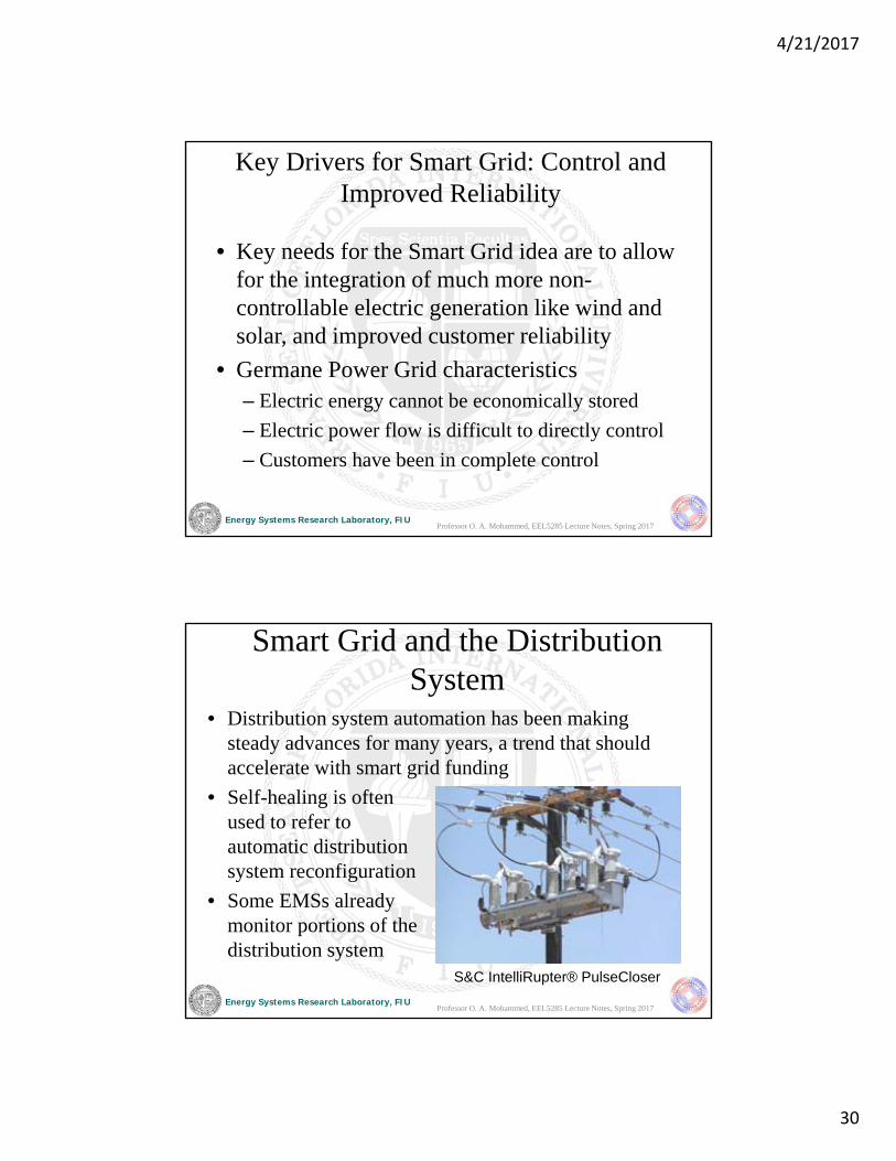
Key Drivers for Smart Grid: Control and Improved Reliability
• Key needs for the Smart Grid idea are to allow for the integration of much more non-controllable electric generation like wind and solar, and improved customer reliability
• Germane Power Grid characteristics– Electric energy cannot be economically stored
– Electric power flow is difficult to directly control
– Customers have been in complete control
Professor O. A. Mohammed, EEL5285 Lecture Notes, Spring 2017
Energy Systems Research Laboratory, FIU
Smart Grid and the Distribution System
• Distribution system automation has been making steady advances for many years, a trend that should accelerate with smart grid funding
• Self-healing is oftenused to refer toautomatic distributionsystem reconfiguration
• Some EMSs alreadymonitor portions of thedistribution system
S&C IntelliRupter® PulseCloser
Professor O. A. Mohammed, EEL5285 Lecture Notes, Spring 2017

4/21/2017
31
Energy Systems Research Laboratory, FIU
Smart Grid and Controllable Load
• A key goal of the smart grid is to make the load more flexible (controllable). One advantage (to utilities) of smart meters is the ability to remotely disconnect folks.
• This requires 1) two-way communication, and 2) at least some loads equipped with controls
• The best methods for achieving this control are still being considered. Communications is key, with the “last mile” the key challenge.
• Potential options are 1) use existing customer broadband connections, 2) broadband over power line (BPL), 3) meshed wireless
Professor O. A. Mohammed, EEL5285 Lecture Notes, Spring 2017
Energy Systems Research Laboratory, FIU
The Smart Grid and the Consumer
• Initially for some consumers the smart grid may just being able to see how they use electricity; but this requires dollars for smarter meters
And translatingthis informationinto real savingsmay be more difficult thansome think
Professor O. A. Mohammed, EEL5285 Lecture Notes, Spring 2017

4/21/2017
32
Energy Systems Research Laboratory, FIU
Pluggable Hybrid Electric Vehicles (PHEVs)
• The real driver for widespread implementation of controllable electric load could well bePHEVs.
• Recharging PHEVs when their drives return home at 5pm would be a really bad idea, so some type of load control is a must.
• Quick adoption of PHEVs depends on gas prices, but will take many years at least
Professor O. A. Mohammed, EEL5285 Lecture Notes, Spring 2017
Energy Systems Research Laboratory, FIU
Duration and Costs of Blackouts
• Cost of blackouts is difficult to determine since electricity has vastly different values. Typical values for a one hour blackout range from a few dollars per kW for residential customers to up to one hundred for industrial and commercial customers.
• Average is several hours of outages per year with the fast majority of the outages due to distribution issues. Weather accounts for about 70% of blackouts, with most affecting a relatively small number of customers.
http://www.eei.org/ourissues/electricitydistribution/Documents/UndergroundReport.pdf
Professor O. A. Mohammed, EEL5285 Lecture Notes, Spring 2017