Surplus Allocation for the Internal Rate of Return Model." Resolving the Unresolved Issue

Daniel F. Gogol, Ph.D., ACAS

115

SURPLUS ALLOCATION FOR THE INTERNAL RATE OF RETURN MODEL:

RESOLVING THE UNRESOLVED ISSUE

Abstract

In this paper, it is shown that with a certain definition of risk-based discounted loss

reserves and a certain method of surplus allocation, there is an amount of premium for a

contract which has the following properties:

(1 .) It is the amount of premium required for the contract to neither help nor hurt the

insurer's risk-return relation.

(2.) It produces an internal rate of return equal to the insurer's target return.

If the insurer gets more than this amount of premium, then the insurer can get more return

with the same risk by increasing the percentage of the premium for the overall book

which is in the segment. Conversely, if the insurer gets less than this amount of

premium, the insurer can increase its return by decreasing the percentage of the overall

premium which is in the segment. The amount of premium is equal to the risk-based

premium in "Pricing to Optimize an Insurer's Risk-Return Relation," (PCAS 1996).

The above property 1 of risk-based premium is proven by Theorem 2 of the 1996 PCAS

paper and not by the present paper. The present paper proves property 2.

116

1. INTRODUCTION

The problem of relating pricing to the risk-return relation has been discussed in many

recent actuarial papers. Surplus allocation is not described in these papers as something

that can be done in a theoretically justifiable way. Actually, though, surplus allocation

has been used in a way that has been proven by a theorem (Theorem 2 of [1]) to derive

the amount of premium for any contract which will neither improve nor worsen the

insurer's risk-return relation. Certain estimates have to be used of course, e.g.

covariances and expected losses. The precise mathematical relationship between this

premium and the risk-return relation is specified by the statement of Theorem 2. This

theorem, and the corresponding definition of risk-based premium, are very rarely

mentioned in recent papers relating pricing to the risk-return relation.

Since the internal rate of return (IRR) model has been a part of the CAS exam syllabus

for years, and since it is a widely used method in insurance and other industries, it may be

possible to explain the method of [1] to a larger group of readers by relating it to the IRR

method.

The IRR model can be used to measure the rate of return for an insurance contract or a

segment of business, but only if the method used for allocating surplus can be related to

the insurer's risk-return relation. The model is generally presented without a

theoretically justifiable method of allocating surplus. But if an arbitrary method of

allocation (such as allocating in proportion to expected losses) is used, the results are

almost meaningless. The purpose of this paper is to complete the IRR method.

Incidentally, there are several actuarial papers which argue that surplus allocation doesn't

make sense because risk is not additive, or because in the real world all of surplus is

available to support all risks. Actually, just as a function f(x) associates each number x

with another number, surplus allocation is a mathematical function which associates each

member of a set of risks with a portion of sttrplus. This function can be used as a part of

a chain of reasoning in order to prove a theorem, as was done in Theorem 2 of [ 1 ].

117

Although surplus allocation was used in deriving the properties of risk-based premium in

[1 ], the derivation doesn't actually require any mention of surplus allocation. When risk-

based premium is related to the IRR method in section 4 of this paper, surplus allocation

is used because that is the traditional way of explaining the IRR method.

The approach presented here:

(1 .) addresses the risk-return relation in a fundamental way

(2.) addresses the problems of the time value of money and the discounting of losses

(3.) addresses the problem of loss reserve risk

(4.) assigns a risk-based premium to the sum of two contracts or segments which

equals the sum of the individual risk-based premiums

The premium derived in this paper by the 1RR method is the same as that determined by

the method in [1] The method in [1] is simpler to apply, but the IRR model has the

advantage of being widely used and understood. It is on the CAS syllabus and has also

been used by non-actuaries for many years. In order to relate the method in [1] to the

1RR method, explanations will be given of both methods. However, since both methods

are explained at length in the literature (see [2],[3],[4]), the explanations will be brief and

informal. This could actually be an advantage, since it could make the presentation more

lively and readable. The part of the paper which is new is the derivation of the

equivalence of the two methods, given certain assumptions and conditions.

118

2. THE IRR MODEL

The IRR model is a method of estimating the rate of return from the point of view of the

suppliers of surplus. Suppose for example that an investor supplied $100 million to

establish a new insurer, and that $200 million in premium was written the next day. Also

suppose that twenty years later the insurer was sold for $800 million. Ignoring taxes, the

return r to the investor satisfies the equation $100 million (1+020 = $800 million.

Therefore, the return r equals 10.96%.

Suppose that, beginning at the time of the above initial investment, each dollar of surplus

is thought of as being assigned to either an insurance policy currently in effect, a loss

reserve liability, or some other risk. Suppose that a cash flow consisting of premium,

losses, expenses, outflows of surplus, and inflows of surplus, is assigned to each policy in

such a way that the following is satisfied: the total of all the cash flows minus the

outstanding liabilities immediately prior to the time at which the above insurer is sold for

$800 million produces an $800 million surplus. It is then possible to express the input of

$100 million, and the payback of $800 million twenty years later, as the total result of the

individual cash flows assigned to each policy. Based on the individual cash flows, the

overall return of 10.96% could then be expressed as a weighted average of individual

returns for each policy. The individual return for a policy is called its intemal rate of

return. The following example is taken from [2].

An Equity Flow Illustration

A simplified illustration of an insurance internal rate of return model should clarify the

relationships between premium, loss, investment, and equity flows. There are no taxes or

expenses in this heuristic example. Actual Internal Rate of Return models, of course,

must realistically mirror all cash flows.

!19

Suppose an insurer

• collects $1,000 of premium on January 1, 1989,

• pays two claims of $500 each on January 1, 1990, and January 1, 1991,

• wants a 2:1 ratio of undiscounted reserves to surplus, and

• earns 10% on its financial investments.

The internal rate of return analysis models the cash flows to and from investors. The

cash transactions among the insurer, its policyholders, claimants, financial markets, and

taxing authorities are relevant only in so far as they affect the cash flows to and from

investors.

Reviewing each of these transactions should clarify the equity flows. On January 1,

1989, the insurer collects $1,000 in premium and sets up a $1,000 reserve, first as an

unearned premium reserve and then as a loss reserve. Since the insurer desires a 2:1

reserves to surplus ratio, equity holders must supply $500 of surplus. The combined

$1,500 is invested in the capital markets (e.g., stocks or bonds).

At 10% per annum interest, the $1,500 in financial assets earns $150 during 1989, for a

total of $1,650 on December 31, 1989. On January l, 1990, the insurer pays $500 in

losses, reducing the loss reserve from $1,000 to $500, so the required surplus is now

$250.

The $500 paid loss reduces the assets from $1,650 to $1,150. Assets of $500 must be

kept for the second anticipated loss payment, and $250 must be held as surplus. This

leaves $400 that can be returned to the equity holders. Similar analysis leads to the $325

cash flow to the equity holders on January 1, 1991.

120

Thus, the investors supplied $500 on 1/1/89, and received $400 on 1/1/90 and $325 on

1/1/91. Solving the following equation for v

$500 = ($400)(v) + ($325)(v ~)

yields v = 0.769, or r = 30%. (V is the discount factor and r is the annual interest rate, so

v = 1/(l+r).)

The internal rate of return to investors is 30%. If the cost of equity capital is less than

30%, the insurer has a financial incentive to write the policy.

This concludes Feldblum's example. My only attempt to improve this simplified

illustration is the following. The $1,000 reserve set up on January I, 1989 is an unearned

premium reserve and by the end of 1989 there is a $1,000 loss reserve. In between, the

sum of the unearned premium reserve and the loss reserve is always $1,000.

Feldblum doesn't claim that the method of surplus allocation in the illustration can be

directly related to the risk-return relation. Allocating in proportion to expected losses

doesn't distinguish between the riskiness of unearned premium, loss reserves, property

risks, casualty risks, catastrophe covers, excess layers, and ground-up layers, for

example. Different methods of surplus allocation could be judgmentally applied to

different types of contracts, but from a theoretical risk-return perspective a certain use of

covariance is required. This will be explained in the next section.

121

3. RISK-BASED PREMIUM

What follows is an informal explanation of the derivation in [1] o f the properties of risk°

based premium. In the discussions below of an insurer's risk-return relation over a one

year time period, "return" refers to the increase in surplus, using the definition of surplus

below. (The term "risk-based discounted" is used in the definition and will be explained

later.)

surplus = market value of assets - risk-based discounted loss and loss adjustment reserves

- market value of other liabilities (3.1)

At any given time, the return in the coming year is a random variable. ] 'he variance of

this random variable is what we refer to by the term "risk". The expression ~'optimizing

the risk-return relation" is used in the same way that Markowitz [5] used it, i.e.,

maximizing return with a given risk or minimizing risk with a given return. (Markowitz

was awarded the Nobel Prize several years ago for his work on optimizing the risk-return

relation o f asset portfolios.)

For an insurance contract, or for a segment of business, the risk-based premium can be

expressed as follows: (The term "loss" will be used for "loss and loss adjustment

expense.")

risk-based premium = expense provision + risk-based discounted losses + risk-based

profit margin. (3.2)

122

The above expense provision is equal to expected expenses discounted at a risk-free rate.

The starting time T for discounting recognizes the delay in premium collection.

Expenses are considered to be predictable enough so that the risk-free rate is appropriate.

The risk-based discounted loss provision is equal to the sum of the discounted values,

using a risk-free rate and the above time T, of

(a.) the expected loss payout during the year

(b.) the expected discounted loss reserve at year-end, discounted as of year-end at

a "risk-based" (not "risk-free') discount rate

A risk-free rate is used to discount (a) and (b) above because the risk arising from the fact

that (a) and (b) may differ from the actual results is theoretically correctly compensated

by the risk-based profit margin (see (3.2) above).

The phrase "contract or segment of business" will be replaced below by "contract", since

the covariance method used below has the following property: the risk-based premium

for a segment equals the sum of the risk-based premiums of the contracts in the segment.

At the inception of an insurance policy, the payout of losses during the year that the

contract is effective, and the estimated risk-based discounted loss reserve for the contract

at the end of the year, are unknown. The effect of the contract on surplus at the end of

the year, i.e., the difference in end of year surplus with and without the contract, can be

thought of as a random variable X at inception. The insurer's return, i.e., the increase in

surplus during the year, is also a random variable. Call it Y.

Assuming that the contract premium equals the risk-based premium, the expected effect

of the contract on surplus at the end of the year is equal to the accumulated value, at the

risk-free interest rate, of the risk-based profit margin. This is true because the expense

provision portion of the formula (3.2) above pays the expenses, and the risk-based

discounted losses portion pays the losses during the year and also accumulates at risk-

free interest, to the expected value of the risk-based discounted loss reserves at the end of

the year. Therefore, by formulas (3.1) and (3.2), above, the effect of the contract equals

the accumulated value of the risk-based profit margin.

123

The random variables X and Y were defined above. If

Cov(X,Y)/Var(Y)=E(X)/E(Y) (3.3)

then, according to Theorem 2 of [1], the contract neither improves nor worsens the risk-

return relation, in a certain sense. This was defined above in the abstract. Note that

E(X), above, equals the accumulated value of the risk-based profit margin.

One of the components of risk-based premium is the expected value of the risk-based

discounted loss reserves at the end of the year. This expected value is greater than the

expected value of the loss reserves discounted at the risk-tree rate corresponding to the

duration of the loss reserves. This is how the risk-based premium provides a reward for

the risk of loss reserve variability. The risk-based discount rate is therefore less than the

risk-free rate.

At the end of each year following the effective period of a contract, if the matching assets

for the risk-based discounted loss reserves are invested at the risk-tree rate~ their expected

value at the end of the following year will be greater than the expected discounted

liability. This is because the risk-based discount rate is less than the risk-free rate.

Assume, for example, that the loss payout is exactly equal to the expected loss payout.

At the moments that loss payments are made, both the discounted loss reserve and the

matching assets are reduced by the same amount. At other times, the matching assets are

growing at the risk-free rate and the discounted liability is growing at the lower risk-

based discount rate.

At the beginning of the second year after the inception of the policy, the end of the year

matching assets minus the discounted loss reserve can be thought of as a random variable

Z. If Cov(Y,Z)/Var(Y) is equal to E(Z)/E(Y), then, according to Theorem 2 of [1], the

risk-based discounted loss reserve and matching assets neither improves nor worsens the

risk-return relation for the year. It is possible to compute a discount rate before the

inception of the contract such that Cov(Y,Z)/Var(Y) is equal to E(Z)/E(Y). Note that if

124

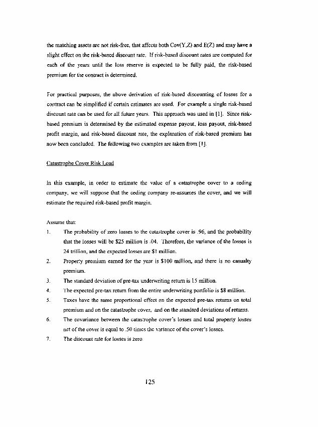
the matching assets are not risk-flee, that affects both Cov(Y,Z) and E(Z) and may have a

slight effect on the risk-based discount rate. If risk-based discount rates are computed for

each of the years until the loss reserve is expected to be fully paid, the risk-based

premium for the contract is determined.

For practical purposes, the above derivation of risk-based discounting of losses for a

contract can be simplified if certain estimates are used. For example a single risk-based

discount rate can be used for all future years. This approach was used in [1]. Since risk-

based premium is determined by the estimated expense payout, loss payout, risk-based

profit margin, and risk-based discount rate, the explanation of risk-based premium has

now been concluded. The following two examples are taken from [1].

Catastrophe Cover Risk Load

In this example, in order to estimate the value of a catastrophe cover to a ceding

company, we will suppose that the ceding company re-assumes the cover, and we will

estimate the required risk-based profit margin.

Assume that:

1. The probability of zero losses to the catastrophe cover is .96, and the probability

that the losses will be $25 million is .04. Therefore, the variance of the losses is

24 trillion, and the expected losses are $1 million.

2. Property premium earned for the year is $100 million, and there is no casualty

premium.

3. The standard deviation ofpre-tax underwriting return is 15 million.

4. The expected pre-tax retum from the entire underwriting portfolio is $8 million.

5. Taxes have the same proportional effect on the expected pre-tax returns on total

premium and on the catastrophe cover, and on the standard deviations of returns.

6. The covariance between the catastrophe cover's losses and total property losses

net of the cover is equal to .50 times the variance of the cover's losses.

7. The discount rate for losses is zero.

125

8. Total underwriting return, and the return on the catastrophe cover, are statistically

independent of non-underwriting sources of surplus variability.

It follows from 1, 6 and 8 above, and from the fact that Cov(X,Y+Z) = Cov(X,Y) +

Cov(X,Z), that the covariance with surplus of the pre-tax return on the catastrophe cover

is 24 trillion + .50(24 trillion); i.e., 36 trillion. It follows from 3 and from Cov(X,Y+Z) =

Cov(X,Y)+Cov(X,Z) that the corresponding covariance for total underwriting is (15

million) 2 , i.e., 225 trillion. Therefore, it follows from assumption 4 that the risk-based

profit margin for the catastrophe cover should be such that the pre-tax return from re-

assuming the catastrophe cover is given by (36/225)($8 million)= $1.28 million. (This is

greater than the cover's expected losses.) If the cover costs more than $2.28 million, then

it improves the insurer's risk-return relation to re-assume it. However, the cover may be

necessary to maintain the insurer's rating and policyholder comfort.

Required Profit Margin by Layer

Suppose that for some insurer:

1.

2.

3.

4.

5.

6.

7.

All premium is property premium.

The accident year expected property losses for the $500,000 excess of $500,000

layer, and the 0-$500,000 layer, respectively, are $10 million and $90 million.

Expected losses excess of $1 million are zero.

The accident year property losses for each of the above layers are independent of

all non-underwriting sources of surplus variation.

The discount rate is zero.

The coefficients of variation (ratios of standard deviations to means) of the higher

and lower layers are .30 and .15, respectively.

The correlation between the two layers is .5.

Taxes have the same proportional effect on th e returns of both layers.

126

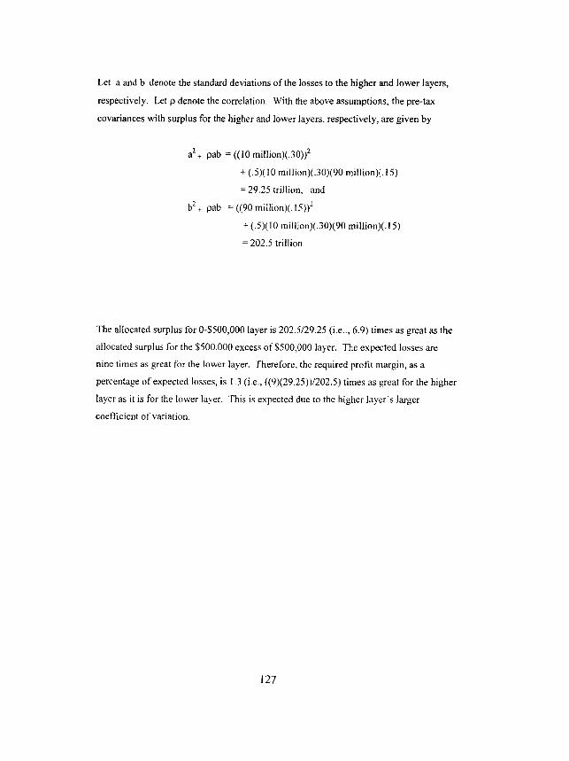
Let a and b denote the standard deviations of the losses to the higher and lower layers,

respectively. Let 13 denote the correlation. With the above assumptions, the pre-tax

covariances with surplus for the higher and lower layers, respectively, are given by

a 2 + pab = ((10 million)(.30)) 2

+ (.5)(10 million)(.30)(90 million)(. 15)

= 29.25 trillion, and

b2+ pab = ((90 million)(.15)) 2

+ (.5)(10 million)(.30)(90 million)(.15)

= 202.5 trillion

The allocated surplus for 0-$500,000 layer is 202.5/29.25 (i.e.., 6.9) times as great as the

allocated surplus for the $500,000 excess of $500,000 layer. The expected losses are

nine times as great for the lower layer. Therefore, the required profit margin, as a

percentage of expected losses, is 1.3 (i.e., ((9)(29.25))/202.5) times as great for the higher

layer as it is for the lower layer. This is expected due to the higher layer's larger

coefficient of variation.

127

4. RISK-BASED PREMIUM AND THE IRR MODEL

An example is given below to show the following, Suppose that the risk-based premium

of my model, for a certain contract corresponds to a certain expected rate of return for the

insurer. Then, the expected rate of return for the contract, using the IRR model, also

equals that target rate if the method of allocating surplus for the IRR model is the

covariance method of my model.

Suppose the target rate of return is 15%. The risk-based premium for a contract equals

expense provision + risk-based profit margin + risk-based discounted losses. Suppose

that premium and expenses are paid at the end of the year, and the expected loss payout is

$100 at the end of each year for four years. Suppose expenses are $70 and the risk-based

profit margin is $30. Suppose that the risk-based discount rate is 4%. It then follows that

the risk-based discounted losses at the end of the year equal $377.51 and the risk-based

premium equals $70 + $30 + $377.51, or $477.51,

By the words surplus and return, I will mean them as defined in my model. The portion

of surplus allocated to the contract for the first year will be called S~ and, using (3.3), it

equals

(Surplus)((Covariance(Contract's After-Tax Underwriting Return, Surplus))/(Variance of

Surplus))

It is possible to estimate the taxes corresponding to underwriting return at the end of the

year of a contract, and the taxes corresponding to the return on risk-based discounted loss

reserves and matching assets in the following years. The effect on taxes of premium

earned, expenses incurred, investment income from premium, and losses paid during the

year, as well as the effect of loss reserves discounted at the beginning and the end of the

year, can be used. In the case of risk-based discounted loss reserves and matching assets,

the expected taxes are less than taxes on the matching assets. This is because loss

rcscrves are discounted from a point in time one year later at the end of the year than at

128

the beginning of the year, producing a loss for tax purposes. If the discount rate used for

tax purposes equals the risk-free rate, but the tax law payout rate is faster than the actual

payout rate, the tax effect is the same as the effect of using the actual payout rate and a

certain discount rate which is lower than the risk-free rate.

Assume for simplicity that the insurer's assets earn 6% for the period of the coming year

and that the tax produced by each type of return is 35% of the return. Then, the above

$30 risk-based profit margin and the above allocated surplus Sj satisfy the equation

.15Si =.65(.06S1+30)

since the 15% target return on allocated surplus is produced by the remainder, after 35%

tax, of 6% investment income on allocated assets plus the $30 risk-based profit margin.

Solving the equation gives Sl = $175.68.

The surplus allocated for the second year equals

(Surplus)((Covariance(Contract's After Tax Loss Reserve Return, Surplus))/(Variance of

Surplus))

This allocated surplus will be called $2. The amount of surplus allocated the next two

years are defined similarly and will be called $3 and $4.

The risk-based discounted loss reserve corresponding to $2 equals $277.51 and satisfies

the equation

.15S2 = .65(.06S2 + (.06 -.04)$277.51) = .65(.06S2 + 5.55)

since the 15% return is equal to the after-tax return from investment income from the

allocated assets plus the after-tax return on loss reserves and matching assets. The

129

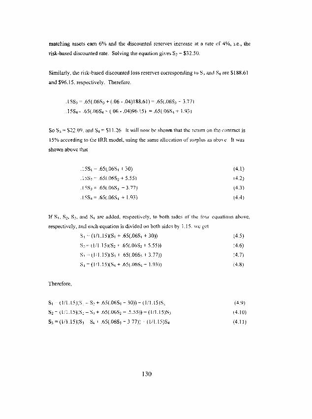
matching assets earn 6% and the discounted reserves increase at a rate o f 4%, i.e., the

risk-based discounted rate. Solving the equation gives $2 = $32.50.

Similarly, the risk-based discounted loss reserves corresponding to $3 and $4 are $188,61

and $96.15, respectively. Therefore,

.15S3 - .65(.06S3 + (.06 - .04)188.61) = .65(.06S3 + 3.77)

.15S~- ,65(.06S4 + (.06 - .04)96.15) = .65(.06S4 + 1.93)

So $3 = $22.09, and $4 = $11.26. It will nov,' be shown that the rctum on the contract is

15% according to the IRR model, using the same allocation o f surplus as above. It was

shown above that

.15SI - . 65 ( ,06S i + 30) (4.1)

.15S2 - .65(,06S2 + 5.55) (4.2)

.15S3 = .65(.06S3 + 3.77) (4.3)

.15S~ - .65(.06S4 + 1.93) (4.4)

If S~, $2, $3, and $4 are added, respectively, to both sides o f the four equations above,

respectively, and each equation is divided on both sides by' 1.15, we get

S~ = ( l / l .15)(Sl + .65(.068~ + 30))

St - ( 1/1.15 )($2 + .65(.06S2 + 5.55))

S~ = (1/1.15)(S~ + .65(.06S3 + 3.77))

$4 - (1/1.15)($4 + .65(.06S4 + 1.93))

(4.5)

(4.6)

(4.7)

(4.8)

Therefore.

Sl = (1/l.15)($1 -- $2 + .65(.06Si + 30)) + (1/1.15)$2

Sz=( l / t . 15 ) (Sz S3+.65( .06S2+.5 .55) )+(1 /1 .15)$3

$3 = (1/1 .15)($3- $4 + .65(.06S3 + 3,77)) + (1/1.15)$4

(4.9)

(4.10)

(4.11)

130

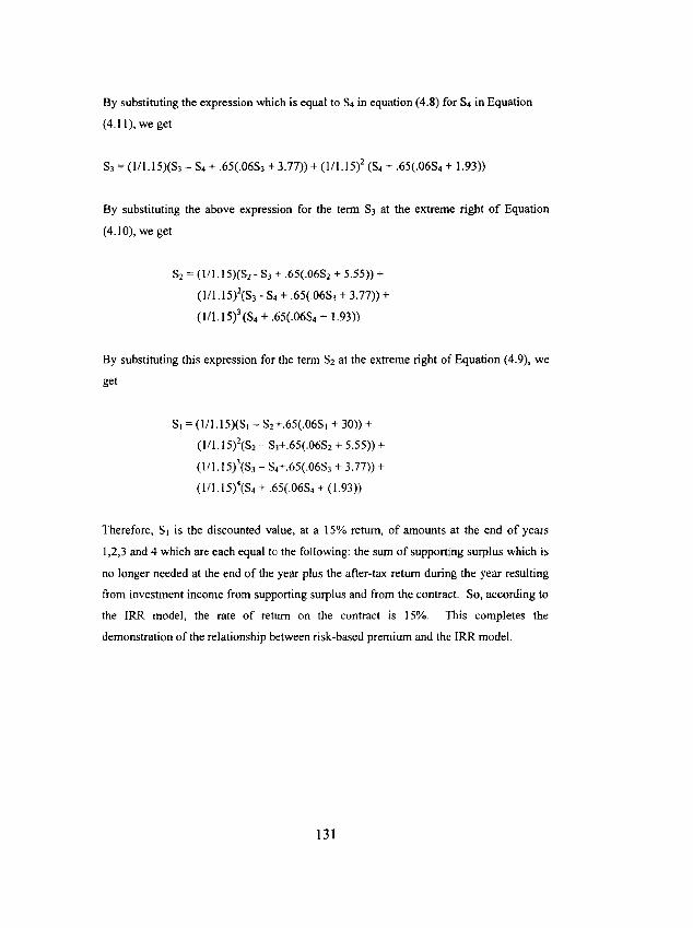
By substituting the expression which is equal to $4 in equation (4.8) for $4 in Equation

(4. l l), we get

$3 = (1/1.15)($3 - $4 + .65(.06S3 + 3.77)) + (1/1.15) 2 ($4 + .65(.06S4 + 1.93))

By substituting the above expression for the term $3 at the extreme right of Equation

(4.10), we get

$2 = (1/1.15)($2- $3 + .65(.06S2 + 5.55)) +

(1/1.15)2($3 - $4 + .65(.06S3 + 3.77)) +

(1/1.I 5) 3 ($4 + .65(.06S4 + 1.93))

By substituting this expression for the term $2 at the extreme right of Equation (4.9), we

get

Sl = (l/1.15)(Sl - $2 +.65(.06St + 30)) +

(1/1.15)z($2 - $3+.65(.06S2 + 5.55)) +

(I/1.15)3($3 - $4+.65(.06S3 + 3.77)) +

(I/1.15)4($4 + .65(.06S4 + (1.93))

Therefore, Sj is the discounted value, at a 15% return, of amounts at the end of years

1,2,3 and 4 which are each equal to the following: the stun of supporting surplus which is

no longer needed at the end of the year plus the after-tax return during the year resulting

from investment income from supporting surplus and from the contract. So, according to

the IRR model, the rate of return on the contract is 15%. This completes the

demonstration of the relationship between risk-based premium and the IRR model.

131

REFERENCES

[I ] Gogol, Daniel F. "Pricing to Optimize an Insurer's Risk-Return Relation," PCAS

LXXXIlI, 1996, pp.41-74.

[2] Feldblum, Sholom, "Pricing Insurance Polices: The Internal Rate of Return

Model," CAS Study Note, May 1992.

[3] Bingham, Russell E., "Surplus - Concepts, Measures of Return, and

Determination," PCAS LXXX, 1993, pp.55-109.

[4] Bingham, Russell E., "Policyholder, Company, and Shareholder Perspectives,"

PCAS LXXX, 1993, pp.110 - 147.

[5] Markowitz, Harry, "Portfolio Selection," The Journal of Finance, March 1952, pp.

77-91.

132