Internal and external variability in regional simulationsdigital.csic.es/bitstream/10261/62232/1/CPD_2011_7_2579.pdf · Internal and external variability in regional simulations

CPD7, 2579–2607, 2011

Internal and externalvariability in regional

simulations

J. J. Gomez-Navarro etal.

Title Page

Abstract Introduction

Conclusions References

Tables Figures

J I

J I

Back Close

Full Screen / Esc

Printer-friendly Version

Interactive Discussion

Discussion

Paper

|D

iscussionP

aper|

Discussion

Paper

|D

iscussionP

aper|

Clim. Past Discuss., 7, 2579–2607, 2011www.clim-past-discuss.net/7/2579/2011/doi:10.5194/cpd-7-2579-2011© Author(s) 2011. CC Attribution 3.0 License.

Climateof the Past

Discussions

This discussion paper is/has been under review for the journal Climate of the Past (CP).Please refer to the corresponding final paper in CP if available.

Internal and external variability in regionalsimulations of the Iberian Peninsulaclimate over the last millenniumJ. J. Gomez-Navarro1, J. P. Montavez1, P. Jimenez-Guerrero1, S. Jerez1,R. Lorente-Plazas1, J. F. Gonzalez-Rouco2, and E. Zorita3

1Departamento de Fısica, Universidad de Murcia, Spain2Departamento de Astrofısica y CC. de la Atmosfera, Universidad Complutense de Madrid,Madrid, Spain3Helmholtz-Zentrum Geesthacht, Geesthacht, Germany

Received: 11 July 2011 – Accepted: 18 July 2011 – Published: 4 August 2011

Correspondence to: J. P. Montavez ([email protected])

Published by Copernicus Publications on behalf of the European Geosciences Union.

2579

http://www.clim-past-discuss.net

http://www.clim-past-discuss.net/7/2579/2011/cpd-7-2579-2011-print.pdf

http://www.clim-past-discuss.net/7/2579/2011/cpd-7-2579-2011-discussion.html

http://creativecommons.org/licenses/by/3.0/

CPD7, 2579–2607, 2011


simulations


Title Page



Tables Figures

J I

J I

Back Close

Full Screen / Esc



Discussion

Paper

|D

iscussionP

aper|

Discussion

Paper

|D

iscussionP

aper|

Abstract

In this study we analyse the role of internal variability in regional climate simulationsthrough a comparison of two regional paleoclimate simulations for the last millennium.They share the same external forcings and model configuration, differing only in theinitial condition used to run the driving global model simulation. A comparison of these5

simulations allows us to study the role of internal variability in climate models at re-gional scales, and how it affects the long-term evolution of climate variables such astemperature and precipitation. The results indicate that, although temperature is ho-mogeneously sensitive to the effect of external forcings, the evolution of precipitationis more strongly governed by random and unpredictable internal dynamics. There10

are, however, some areas where the role of internal variability is lower than expected,allowing precipitation to respond to the external forcings, and we explore the under-lying physical mechanisms responsible. We find that special attention should be paidwhen comparing the evolution of simulated precipitation with proxy reconstructions atregional scales. In particular, this study identifies areas, depending on the season, in15

which this comparison would be meaningful, but also other areas where good agree-ment between model simulations and reconstructions should not be expected even ifboth are perfect.

1 Introduction

The climate system fluctuates naturally over a large frequency range, from days to20

millions of years (Huybers and Curry, 2006). In the context of anthropogenic climatechange, it is important to have available reliable estimations of the amplitude of naturalvariability on multidecadal timescales and at regional spatial scales, since this variabil-ity may hinder the attribution of trends observed to the anthropogenic forcing. On theother hand, the adaptation to anthropogenic climate change at regional scales should25

take into account the existence of potentially large natural variations superposed on

2580





CPD7, 2579–2607, 2011


simulations


Title Page



Tables Figures

J I

J I

Back Close

Full Screen / Esc



Discussion

Paper

|D

iscussionP

aper|

Discussion

Paper

|D

iscussionP

aper|

longer-term climate change. In addition, it can also be affected by anthropogenic green-house gas emissions at multi-decadal scale.

The observational record is too short to reliably assess multidecadal climate varia-tions and therefore the analysis of past climates can help in the estimation of the pastamplitude of variability and of its mechanisms. Efforts to assess the role of natural5

variability belong to two categories: climate reconstructions based on proxy indicatorsand climate model simulations. Comparing both approaches is important to identifysystematic errors in simulations as well as drawbacks in the methodologies used inreconstructions (Gonzalez-Rouco et al., 2009). In particular, the validation of climatemodels in a past climate context may increase the confidence placed in climate change10

projections. Nevertheless several limitations arise when comparing results from mod-els and reconstructions.

One drawback is the scale gap between both approaches. Although the use ofcomprehensive atmosphere-ocean global circulation models (AOGCMs) has becomepossible due to the impressive increase in computational power (Zorita et al., 2005;15

Tett et al., 2007; Ammann et al., 2007; Swingedouw et al., 2010; Jungclaus et al.,2010, among others), their spatial resolution is still too coarse to take into account theregional climate features caused by fine orographic details. Climate reconstructionsare thought to be very sensitive to these details, which are implicit in the informationextracted from the proxies. This scale gap may be bridged using Regional Circulation20

Models (RCMs), which simulate the climate system for a limited domain (Kittel et al.,1998; Jerez et al., 2010, among others). This downscaling approach is commonly usedin climate change projections (Jacob et al., 2007; Deque et al., 2007; Gomez-Navarroet al., 2010, among many others), but to date there are few studies focusing on theapplications of RCMs in a paleoclimate context (Zorita et al., 2010; Gomez-Navarro25

et al., 2011; Strandberg et al., 2011).Another important limitation in the model-proxy comparison is the inherent internal

variability of climate models. Just like the actual climate, the models are affected bya strong chaotic internal variability over a broad band of time scales. This implies

2581





CPD7, 2579–2607, 2011


simulations


Title Page



Tables Figures

J I

J I

Back Close

Full Screen / Esc



Discussion

Paper

|D

iscussionP

aper|

Discussion

Paper

|D

iscussionP

aper|

that a complete agreement at interannual timescales should not be expected whencomparing the temporal evolution of model simulations and reconstructions, even ifboth are perfect (Yoshimori et al., 2005). Furthermore, the magnitude of this internalvariability as well as its importance in the evolution of the simulations is not well known,at least until now.5

In this the study, we present a comparison of two simulations performed with a cli-mate version of the mesoscale model MM5 driven by the AOGCM ECHO-G over thelast millennium (1001–1990) for a domain encompassing the Iberian Peninsula (IP).The model configuration and the external forcings are the same in both simulations.The only difference lies in the initial condition used to run the two simulations in the10

global model, and thus these experiments allow us to investigate the role of externalforcing in the evolution of several climate variables compared to the magnitude of theinternal variability of the model at regional scale. We focus on the evolution of near-surface air temperature (SAT) and precipitation (PRE) in winter (mean of December-January-February) and summer (mean of June-July-August).15

2 Description of the simulations

The global model ECHO-G driving the RCM consists of the spectral atmospheric modelECHAM4 coupled to the ocean model HOPE-G (Legutke and Voss, 1999). The modelECHAM4 was used with a horizontal resolution T30 (∼3.75◦ ×3.75◦) and 19 verticallevels. The horizontal resolution of the ocean model is approximately 2.8◦ ×2.8◦, with20

a grid refinement in the tropical regions and 20 vertical levels. Two simulations wereperformed with this model configuration, both driven by the same reconstructions ofseveral external forcings, which are depicted in the first two panels of Fig. 1. Blue, pink,and grey lines represent the evolution of atmospheric carbon dioxide, nitrous oxide, andmethane, respectively. The orange line represents the reconstruction employed for the25

variability of the total solar irradiance (TSI). Black lines show the estimated equivalentreduction in solar irradiance at the top of the atmosphere caused by volcanic eruptions.

2582





CPD7, 2579–2607, 2011


simulations


Title Page



Tables Figures

J I

J I

Back Close

Full Screen / Esc



Discussion

Paper

|D

iscussionP

aper|

Discussion

Paper

|D

iscussionP

aper|

The sum of both lines is the effective solar constant, which is implemented in the modelto take into account both sources of short-wave external forcing. The two simulations(hereafter referred as ERIK1 and ERIK2) cover the last millennium almost entirely,and the only difference between them is the initial condition (ERIK2 is colder). A fulldescription of these simulations can be found in Gonzalez-Rouco et al. (2003); Zorita5

et al. (2005) and references therein.The RCM used to downscale the two AOGCM simulations is a climate version of the

Fifth-generation Pennsylvania-State University-National Center for Atmospheric Re-search Mesoscale Model (Dudhia, 1993; Grell et al., 1994; Montavez et al., 2006;Gomez-Navarro et al., 2010). A double-nesting scheme was implemented, with10

a lower-resolution (90 km) outer domain covering Western Europe and a higher-resolution (30 km) inner domain covering the IP. Both domains are two-way coupled.These domains, as well as the chosen physical parametrisation, are the same as thosepreviously described by Gomez-Navarro et al. (2011). The regional simulations havebeen driven with exactly the same external forcing reconstructions as in the global15

model simulations to avoid physical inconsistencies. The two downscaled simulations,which cover the period 1001–1990, will be referred hereafter as MM5-ERIK1 and MM5-ERIK2, respectively.

3 Results

3.1 Correlation as a measure of internal variability20

Figure 1 depicts the evolution of the anomalies in SAT and PRE in winter and sum-mer averaged over the IP in the two RCM simulations. The eight series have beensmoothed with a 31 yr running mean in order to filter out the high frequency signal andhighlight the low-frequency variability. In the SAT series we can easily identify threemain periods: a warm initial condition up to roughly 1400, followed by a long cold period25

which finishes around 1850, reverting to a stronger trend towards a warmer climate.

2583





CPD7, 2579–2607, 2011


simulations


Title Page



Tables Figures

J I

J I

Back Close

Full Screen / Esc



Discussion

Paper

|D

iscussionP

aper|

Discussion

Paper

|D

iscussionP

aper|

These periods match the already known characteristic periods in the last millenniumsuch as the Medieval Optimum, the Little Ice Age, and the warmth of the IndustrialAge. In particular, there are some noticeable cold periods such as the Sporer Mini-mum (around 1450), the Maunder Minimum (around 1700), and the Dalton Minimum(around 1810) which can be identified in the SAT series and may be associated with a5

simultaneous reduction in the TSI and volcanic activity. The final trend can be linked toan increase not only in the TSI but also with the large increase in GHG concentrations.In general terms, the impact of the external forcing in these cold periods seems to bemore relevant in summer in both simulations, which exhibit good agreement in termsof variability and temporal evolution.10

The fingerprint of the forcings in the evolution of PRE is, however, less apparent.Other than a slight decrease in precipitation, more noticeable in summer seasons since1800 to the end of the simulation, it is not easy to identify the impact of variations inthe external forcing. Further, although the variability depicted by both simulations issimilar in both seasons, their temporal agreement is lower than in the case of SAT,15

suggesting a stronger independence of PRE of the external forcings. The variability ofwinter precipitation is stronger, as corresponds to the wetter conditions in this seasonin the IP, a feature correctly reproduced by both simulations.

Careful comparison of these two millennial simulations allows the study of the in-ternal variability through the quantification of the signal-to-noise ratio. This can be20

assessed through the time correlation of the temporal evolution of different variables inthe two experiments. A simple conceptual model of the evolution of a climate variablethat is partially driven by the external forcing may illustrate this point. The variable canbe considered as a combination of the external forcing plus a contribution of noise dueto the inherent chaotic nature of the simulation:25

T =αW + f (1)

where T is the variable of interest, α is a proportionality constant, W is noise represent-ing internal variability, and f the direct effect of the external forcing in the variable. If wenow perform several identical simulations, only differing in the initial condition, we have

2584





CPD7, 2579–2607, 2011


simulations


Title Page



Tables Figures

J I

J I

Back Close

Full Screen / Esc



Discussion

Paper

|D

iscussionP

aper|

Discussion

Paper

|D

iscussionP

aper|

several variables Ti . The point here is that random noise prevents correlation betweenthese variables from being perfect. Instead, the correlation between these variablescan be depicted as:

cor(Ti ,Tj )=Var(f )

Var(f )+α2(2)

where the variance of the variable is assumed to be the same in all the experiments5

(i.e. Var(Ti ) = Var(Tj ), ∀i ,j ) and W and f are uncorrelated. Hence, according to thelast equation, if forcing plays a strong role in the evolution of T , α can be considerednegligible and the correlation is close to one. On the other hand, if the evolution of thevariable depends strongly on the internal variability (α is large), the right term in Eq. (2)becomes small and the evolution of the variable is not correlated between the different10

experiments. Thus, the correlation gives a quantitative measure of the relative role ofinternal variability in the evolution the different variables of the simulation, a parameterthat will be used in the next section.

It is important to note, nonetheless, that the influence of the external forcing detectedin this way may be dependent on the time scale, season, and area. This is due to the15

different amplitude of internal variability, from daily to interdecadal, and to the amplitudeof the external forcing at different time scales. In this study we have performed ananalysis using different running means with increasing time intervals in an attempt toidentify the temporal scales at which the signal-to-noise ratio is stronger.

3.2 Forced vs. unforced evolution of SAT and PRE20

Figure 2 depicts the spatial distribution of the correlation between the SAT series sim-ulated in the MM5-ERIK1 and MM5-ERIK2 experiments, both smoothed using threedifferent running means. The evolution of this variable in the two experiments is highlycorrelated in both seasons (black circle denotes grid points where the correlation is sig-nificant at the 95 % confidence level according to a bootstrap method (Ebisuzaki, 1997),25

and it is quite steady over the domain. Correlation in summer is slightly stronger, and2585





CPD7, 2579–2607, 2011


simulations


Title Page



Tables Figures

J I

J I

Back Close

Full Screen / Esc



Discussion

Paper

|D

iscussionP

aper|

Discussion

Paper

|D

iscussionP

aper|

in both seasons tends to be somewhat greater when a stronger smoothing is applied.It is interesting to note that the spatial structure of the correlation is different in winterand summer, with stronger correlations in the southern part of the IP in summer, andstronger correlations in the north in winter. There are hardly any changes when differ-ent running means are applied. The main conclusion we can derive from this figure5

is that the evolution of SAT seems to be dependent on the evolution of the externalforcings, and this result is valid everywhere in the IP. This result is quite reasonablesince near-surface temperature should be physically strongly modulated by the exter-nal forcing. The magnitude of the correlation is essentially independent of the degree ofsmoothing, which may be interpreted as the strongest influence of the external forcing10

already being attained at the smallest time scale probed here.Similarly, Fig. 3 depicts the same information for PRE. In this case the correlation

is in general lower and in some cases even negative. There are, however, some welldefined areas where this variable still exhibits a high and statistically significant corre-lation between experiments (denoted with a black circles, as in Fig. 2). As before, the15

correlation structure of winter and summer is different, with only changes in intensityoccurring when a stronger smoothing is applied. In winter, the areas which most clearlyrespond to the forcings are the northeast of the IP and the main mountain systems suchas the Pyrenees and also the Iberian and Betic systems. Conversely, the sensitive ar-eas in summer are located in the west and north of the IP, and show no clear influence20

of the orographic features of the domain. We discuss a possible physical explanationfor these patterns in the next subsection.

When we further analysed the significance of the correlations calculated in the for-mer section and their relationship with the smoothing applied to the series in Fig. 4, themean correlation for SAT was above a 95 % confidence interval in both seasons and25

for all the tested running means, although in winter it tends to be slightly lower. Theresemblance between series increases with longer smoothing, but it saturates around50 years. The limit for the confidence interval increases monotonically with longersmoothing, and is greater for summer when correlations are also higher. Apart from

2586





CPD7, 2579–2607, 2011


simulations


Title Page



Tables Figures

J I

J I

Back Close

Full Screen / Esc



Discussion

Paper

|D

iscussionP

aper|

Discussion

Paper

|D

iscussionP

aper|

the non-smoothed series of winter temperature, nearly all grid points exhibit a corre-lation above the 95 % confidence level, supporting our previous interpretation on theimportance of the external forcings in the evolution of SAT in the IP during the lastmillennium.

From a regional modelling perspective, the results for PRE are especially interest-5

ing. Figure 4 illustrates how the correlations for this variable are, on average, below theconfidence level. Nevertheless, as mentioned above, there are areas where the corre-lation is still high. The dashed bar represents the percentage of grid points in the do-main where the correlation is significant at the 95 % confidence level, and Fig. 3 allowstheir identification in different seasons. It is in these areas where the forcings plays an10

important role in the evolution of precipitation. They can only be identified through theuse of a high resolution model since the average spatial process dilutes the statisticalconfidence, as Fig. 4 clearly illustrates. Another important aspect of these calculationsis that they demonstrate that, although the correlation between experiments tends tobe higher when longer smoothing is applied, the threshold for statistical significance is15

also larger, so that the number of grid points which show a significant correlation doesnot increase monotonically.

3.3 Physical meaning of the correlations

Although statistical significance is a necessary condition, it is not sufficient to assertthat there is a causal relationship between the long-term evolution of forcings and SAT20

and PRE. The physical link between forcing and temperature is straightforward: thestronger the external radiative forcing, the higher the temperature. It depends nei-ther on regional features nor on the season. The correlation map at global scale (notshown) between the external forcings and SAT is homogeneously positive over mostof the globe, independent of the season, and it is similar in magnitude to that shown25

in Fig. 2 for the IP. However, the link between forcing and precipitation is less obvi-ous. In principle, higher temperatures tend to increase the evaporation, and hencethe moisture content of the atmosphere. However, higher temperatures would tend to

2587





CPD7, 2579–2607, 2011


simulations


Title Page



Tables Figures

J I

J I

Back Close

Full Screen / Esc



Discussion

Paper

|D

iscussionP

aper|

Discussion

Paper

|D

iscussionP

aper|

reduce the relative humidity for a given level of moisture, which tends to diminish thecloud cover and precipitation. The net result may depend on the regional features, thelarge-scale circulation, or the season. In fact, we found that the large-scale correla-tion between forcings and PRE shows no clear homogeneous signal over the global(not shown), as in the case of SAT. Thus, the net effect of higher/lower forcings is de-5

pendent on other indirect factors such as modifications in the local circulation or theinteraction with the orography. In addition, this relationship strongly depends on theseason, as illustrated by Fig. 3. For this reason, we have investigated the physicalmechanism linking the evolution of precipitation and forcing separately for winter andsummer, and focusing only in the IP, since in other areas it could be different. In the re-10

maining part of this section we focus on the low-frequency variations, since they showa larger signal-to-noise ratio. To do so, we use a simple low-pass filter which elimi-nates the variability at shorter timescales than 50 yr. We analyse the low-frequencyvariations of SAT and PRE through an Empirical Orthogonal Function (EOF) analysis(Hannachi et al., 2007), a methodology that reduces the high dimensionality of com-15

plex phenomena, such as climate, and has been used in other studies regarding longregional climate simulations (Gomez-Navarro et al., 2010). Finally, since we are inter-ested in the variations relative to the mean state and the precipitation over the IP isstrongly heterogeneous (Serrano et al., 1999), we have used standardised precipita-tion series to avoid an over-representation of the wettest areas in the northwest of the20

IP. Hence, all EOF maps shown here are dimensionless.The first EOF of the normalised low-frequency variations of SAT and PRE in summer

in the experiment MM5-ERIK2 are shown in Fig. 5a and b and explain 89 % and 44 %of the variance, respectively. The corresponding figures for MM5-ERIK1 are very sim-ilar and are not shown here. The associated Principal Components (PCs) for the two25

variables and experiments are shown in Fig. 5d, together with the external forcings.The close relationship between the evolution of SAT and PRE is apparent in the twosimulations. The correlation between the PCs of SAT and PRE is 0.82 and 0.79 forthe MM5-ERIK1 and MM5-ERIK2, respectively. Figure 5c shows the correlation map

2588





CPD7, 2579–2607, 2011


simulations


Title Page



Tables Figures

J I

J I

Back Close

Full Screen / Esc



Discussion

Paper

|D

iscussionP

aper|

Discussion

Paper

|D

iscussionP

aper|

between the low-frequency evolution of the two variables for MM5-ERIK2 (the corre-sponding map for MM5-ERIK1 is similar and has also been omitted), and indepen-dently illustrates the close link between the two variables. The resemblance betweenthe maps in Fig. 5b and c can be better understood by looking at the PCs. The low-frequency variations of SAT are dominated by a spatially homogeneous EOF, whereas5

the variations of PRE display several spatial characteristics. The strong correlation be-tween the PCs, as well as the high percentage of variance that the first EOF for eachvariable explains, drive the clear correlation between these variables and their spatialstructure.

On the other hand, the correlations between the PCs of the two experiments are10

0.81 and 0.34 for SAT and PRE, respectively. This is in good agreement with ourprevious finding of a stronger influence of the external forcings in the evolution of SATthan in the case of PRE. In addition, the similarity between the map in Fig. 5c (orFig. 5b) and correlation maps in Fig. 3 for summer is clear. Again, the explanationfor the structure and intensity of these correlation patterns is better sought in the EOF15

analysis. The homogeneous first EOF, together with the large amount of variabilityit explains and the large correlation between the associated PCs, force a high andhomogeneous correlation between the SAT in the two experiments. On the contrary,the lower correlation between PCs associated with the evolution of PRE in the twoexperiments precludes strong coupling between them. Despite this, the shape of the20

main variability mode is similar in the two simulations, and the correlation between bothPCs is not negligible, which explains why the areas most affected by this pattern standout in the correlation maps of Fig. 3.

Having identified that the response to the forcing in summer precipitation over theIP is due to the main variability mode, which has the same spatial structure and is25

clearly correlated in the two simulations, we sought the physical mechanism behindthis link. First, we separately considered large-scale and convective precipitation. Thecorrelation maps, equivalent to those shown in Fig. 3 for convective precipitation alone,depict very low values and no spatial structure, whereas the maps corresponding to

2589





CPD7, 2579–2607, 2011


simulations


Title Page



Tables Figures

J I

J I

Back Close

Full Screen / Esc



Discussion

Paper

|D

iscussionP

aper|

Discussion

Paper

|D

iscussionP

aper|

large-scale precipitation look very similar to those in Fig. 3 (not shown). This suggeststhat the response to forcing is in the large-scale field, in particular in the response ofregional circulation to external forcings. To confirm this, Fig. 6 shows the correlationbetween the low-frequency filtered series of external forcings and SLP for summer inthe ERIK2 experiment (the map corresponding to ERIK1, not shown, exhibits the same5

pattern and supports the same physical explanation). We show the calculations in theAOGCM fields since this area lies outside the domain simulated by the RCM, and, inany case, the differences between the RCM and the AOGCM in the SLP field are small.This figure shows how the local circulation is affected by the driving forcings. In partic-ular the strengthening of the Azores high reduces the large-scale precipitation over the10

northwest, whereas the low over Morocco has the opposite effect and is responsiblefor the simultaneous increase of precipitation in the southeast of the IP and over theMediterranean Sea, which is precisely the shape of the first EOF shown in Fig. 5b.

The results for winter are different. As discussed above, Fig. 3 shows how the cor-relation structure for winter is different from that of summer, which suggests that the15

underlying physical mechanism may also be different. Figure 7a, b and c are equiv-alent to Fig. 5a, b, and c for winter (as before, the following argument is based onthe MM5-ERIK2 experiment, although it also holds for the MM5-ERIK1 experiment).The evolution of SAT in winter is dominated by a homogeneous EOF, with associatedPCs that are strongly correlated in the two experiments (correlation 0.68). However,20

an important difference between summer and winter is that in the latter, the leadingEOF for precipitation (Fig. 7b) is very different from the correlation pattern betweentemperature and precipitation (Fig. 7c). The explanation for this difference has to besought in the impact of large-scale circulation in the precipitation regime in winter overthe IP. The North Atlantic Oscillation (NAO) is a variability mode of SLP in the North25

Atlantic area that strongly affects the winter precipitation amount in the IP, especiallyin the western parts (Trigo et al., 2004). The MM5-ECHO-G model is able to success-fully reproduce this feature (Gomez-Navarro et al., 2011). Figure 7d illustrates this byshowing the correlation between the NAO index, defined as the PC associated to the

2590





CPD7, 2579–2607, 2011


simulations


Title Page



Tables Figures

J I

J I

Back Close

Full Screen / Esc



Discussion

Paper

|D

iscussionP

aper|

Discussion

Paper

|D

iscussionP

aper|

first EOF of winter SLP in the North Atlantic area, and the PRE series in each gridpoint. It is apparent how the areas most affected by NAO (Fig. 7d) are those standingout in the first EOF of PRE (Fig. 7b). This means that in winter the main variabilitymode of precipitation is dominated by NAO variations. However, the correlation of thelow-frequency variations of NAO in the two simulations is only 0.17 (below 0.27, the5

significance level at the 95 % confidence level), indicating that this important circulationmode does not respond to the external forcing but is dominated by internal variabilityin the AOGCM. This explains the generally lower impact of the driving forcing in theevolution of precipitation in winter. In winter, the fingerprint of the relationship betweenSAT and PRE illustrated in Fig. 7c has to be sought in the second EOF. This is shown10

in Fig. 7e and explains 18 % of the low-frequency precipitation variance once the NAOsignal has been removed by the first EOF. We compare this second most importantvariability mode for winter precipitation with the correlation pattern between SAT andPRE. This mode of precipitation variability, once the influence of the non-forced NAOhas been removed, responds to the forcings, as can be identified by comparing Fig. 7e15

and the correlation maps for winter in Fig. 3. In fact, the correlation between the PCassociated to this precipitation mode and the PC associated with the SAT is 0.62 (0.66in MM5-ERIK1).

The physical link between temperature and precipitation in winter described above,which is responsible for the resemblance between the evolution of the precipitation20

series during this season in the two simulations shown in Fig. 3, is not due to the re-sponse of the large-scale circulation to the external forcings as in the case of summer.Instead, it is due to the interactions between the large-scale circulation and the orogra-phy of the RCM. Figure 8a shows the correlation between the low-frequency evolutionof precipitation series in the two simulations, together with the orography considered25

by the model (in green contours). The correlation is more intense near the main moun-tain systems such as the north side of the Pyrenees or the western part of the Iberianand Betic systems. This figure, together with the characteristic anti-correlation mapbetween temperature and precipitation shown in Fig. 7c, suggests that there may exist

2591





CPD7, 2579–2607, 2011


simulations


Title Page



Tables Figures

J I

J I

Back Close

Full Screen / Esc



Discussion

Paper

|D

iscussionP

aper|

Discussion

Paper

|D

iscussionP

aper|

a modulation in the condensation level, driven by temperature variations, which wouldcould especially affect the precipitation over mountanous regions. To check this, thecondensation level has to be calculated within the simulations. This variable can berelated with the dew point temperature in good approximation by the difference:

CL∝ (T −Td) (3)5

where T is temperature and Td is the dew point temperature, both variables measuredon the surface (Lawrence (2005) presents a modern review on the relations betweenmoisture, temperature, and how they are related). Figure 8b shows the correlationbetween temperature variations and the temperature differences in Eq. (3). There is agenerally strong and positive relation between the height of the condensation level and10

the temperature, which is not an obvious result since the moisture content over the IPdepends to a large extent on the evaporation rate in the Atlantic Ocean which is lowerin colder periods. The relation is stronger near the main mountain systems, althoughthe correlation map also depicts sensitivity to the Atlantic flow on the windward side ofthe mountains. That is, in cold periods the condensation level sinks, especially on the15

windward side of the mountains, and this affects the increase of precipitation in theseareas. Hence, the physical link between precipitation and forcing in winter is throughvariations in the condensation level, directly modulated by variations in temperature.Surprisingly, despite the intensity of the noise due to internal variability in the winterprecipitation, this mechanism is strong enough to leave an observable mark in the20

amount of precipitation in some areas over the IP characterised by the orography. Itis important to note that this mechanism can only be accurately reproduced withinthe context of a high resolution simulation capable of resolving the fine spatial scalesinvolved.

2592





CPD7, 2579–2607, 2011


simulations


Title Page



Tables Figures

J I

J I

Back Close

Full Screen / Esc



Discussion

Paper

|D

iscussionP

aper|

Discussion

Paper

|D

iscussionP

aper|

4 Summary and conclusions

In this study we have compared the evolution of SAT and PRE in two millennial pale-oclimate simulations performed with a RCM with a spatial resolution of 30 km for theIP. The comparison allows us to evaluate the importance and magnitude of the internalvariability in the evolution of these variables relative to the influence of the reconstruc-5

tion of external forcings used to drive the simulations. The underlying argument is thatif external forcings play a weak role in the evolution of the simulation, the temporal cor-relation of the series associated with these variables in both simulations should not alsobe weak since the internal variability, generated by the chaotic nature of the climaticsystem, is uncorrelated in both simulations.10

The results indicate that the long-term evolution of SAT is strongly affected by theexternal forcings driving the simulation. This variable responds homogeneously to theexternal factors over the IP at most temporal scales. The evolution of PRE is, however,more strongly governed by chaotic variability at regional scale. In particular, there arefew a areas in the IP, the main mountain system in winter and the north and west15

areas in summer, where the precipitation is significantly driven by external forcings.However, in many parts of the domain the influence of the external forcing can notbe detected in the evolution of PRE. It is important to note that the significance ofthe correlation emerges at regional scales and is blurred when a spatial average isperformed. This stresses the importance of high resolution simulations in exercises20

comparing the model results with proxy reconstructions of precipitation.The influence of the external forcing on precipitation is especially weak in winter.

This is due to the nature of the winter precipitation over the IP, which is dominated byvariations in the NAO. The NAO seems to be quite insensitive to the external forcing inthe simulations at the investigated timescales. Once the NAO signal is removed from25

the precipitation series, the leading variability pattern corresponds quite well with theareas which are more clearly able to respond to forcings. Precipitation in summer ismore strongly affected by variations in the forcing. Its main variability mode matches

2593





CPD7, 2579–2607, 2011


simulations


Title Page



Tables Figures

J I

J I

Back Close

Full Screen / Esc



Discussion

Paper

|D

iscussionP

aper|

Discussion

Paper

|D

iscussionP

aper|

well the areas where summer precipitation responds to external forcing. In fact, wehave been able to demonstrate that this precipitation mode is dominated by modulationof the large-scale SLP by the external forcing in summer. This is in contrast with thestronger contribution of the internal variability of SLP in winter. During this seasonthere are still some areas where precipitation responds the forcing, but, in this case, it5

is not through modification in the large-scale flow but through the interaction betweencondensation level and orography.

Our findings regarding the impact of internal variability in the simulations may havea strong impact on how comparison between simulations and reconstructions are per-formed. In particular, we have been able to identify areas where we should not expect10

good agreement between the model and the reconstructions, even if both are perfect.On the other hand, there are areas, mostly in the main mountain systems, where mis-matches between both approaches can not be argued to be due to internal variability.These results stress the importance of RCMs in paleoclimate studies, since we havedemonstrated that the physical mechanism responsible for the response of precipita-15

tion to external forcings in winter can only be realistically reproduced by using highresolution simulations.

A further important comment has to be made regarding the reconstructions of solarforcing used in these simulations. The evolution of the TSI used in these simulationsis taken from Crowley (2000). However, a more recent reconstruction of this variable20

(Krivova and Solanki, 2008) depicts a much smaller amplitude of the variations. Inparticular, these authors estimate a difference in total solar irradiance between theLate Maunder Minimum and late 20th century of 1.25 W m−2 (about 0.09 %), whereasthe past solar irradiance used in these simulation changes by 0.3 %. Yet more recentreconstructions of TSI over the Holocene (Shapiro et al., 2011) again points to an even25

wider amplitude of TSI variations than those used in these simulations: 0.4 % changebetween the Late Maunder Minimum and late 20th century. It is beyond the scope ofthis study to analyse which of these reconstructions more realistically represents thepast. The influence on our analysis of using reconstructions with lower amplitude in the

2594





CPD7, 2579–2607, 2011


simulations


Title Page



Tables Figures

J I

J I

Back Close

Full Screen / Esc



Discussion

Paper

|D

iscussionP

aper|

Discussion

Paper

|D

iscussionP

aper|

simulation would be to reduce the term Var(f ) in Eq. (2), and thus reduce the correlationof the same variable between simulations. Higher-amplitude reconstructions of pastTSI would have the opposite effect.

A similar argument could apply to volcanic forcing, for which the uncertainties arestill also large. In addition, the implementation of volcanic forcing in these simulations,5

simply as a reduction in the effective solar constant, possibly precludes a more realisticsimulation of the volcanic winter warming at mid and high-latitudes due to the NAOresponse to differential effect of volcanic aerosols in the Tropics and high latitudes(Stenchikov et al., 2006; Fischer et al., 2007). According to this mechanism, wintersafter volcanic eruptions should experience a stronger NAO and thus the IP would tend10

to receive less precipitation. This mechanism tends to increase the influence of thevolcanic forcing and it would phase-lock the simulated precipitation in both simulationsin periods with intense volcanic activity more strongly than is detected in our simulationset-up.

Finally, some of these conclusions can be extended with caution to the climate15

change projections. In a forced scenario, the SAT can be expected to be influencedby external forcings, and hence their projections present a reasonable degree of con-fidence. Evolution of PRE is nevertheless less reliable since its behaviour at regionalscale is governed by greater uncertainty due to the influence of internal variability. Thisdrawback is an addition to the well known uncertainties characteristic of precipitation20

projections under climate change scenarios (IPCC, 2007). Nevertheless, it has to betaken into account that our findings depend on the intensity of the external forcings. Inclimate change projections the intensity of external forcings is stronger, and thus theoverall role of internal variability can be expected to be lower. In future works, a similarstudy should be carried out with different runs for the same climate change projection.25

Acknowledgements. This work was funded by the Spanish Ministry of the Environ-ment (project SALVA-SINOVAS, Ref. 200800050083542) and the Spanish Ministry ofScience and Technology (project SPECMORE-CGL2008-06558-C02-02/CLI). The authorsalso gratefully acknowledge funding from the Euro-Mediterranean Institute of Water (IEA).

2595





CPD7, 2579–2607, 2011


simulations


Title Page



Tables Figures

J I

J I

Back Close

Full Screen / Esc



Discussion

Paper

|D

iscussionP

aper|

Discussion

Paper

|D

iscussionP

aper|

J. J. Gomez-Navarro thanks the Spanish Ministry of Education for his Doctoral scholarship(AP2006-04100). The work by E. Zorita is embedded in the EU-Project Millennium EuropeanClimate. Thanks to Elena Bustamante for the stimulating discussions.

References

Ammann, C. M., Joos, F., Schimel, D. S., Otto-Bliesner, B. L., and Tomas, R. A.: Solar influence5

on climate during the past millennium: Results from transient simulations with the NCARClimate System Model, Proceedings of the National Academy of Sciences of the UnitedStates of America, 104, 3713–3718, doi:10.1073/pnas.0605064103, 2007. 2581

Crowley, T.: Causes of climate change over the past 1000 years, Science, 289, 270, 2000.259410

Deque, M., Rowell, D. P., Luthi, D., Giorgi, F., Christensen, J. H., Rockel, B., Jacob, D., Kjell-strom, E., de Castro, M., and van den Hurk, B.: An intercomparison of regional climatesimulations for Europe: assessing uncertainties in model projections, Climatic Change, 81,53–70, doi:10.1007/s10584-006-9228-x, 2007. 2581

Dudhia, J.: A Nonhydrostatic Version of the Penn StateNCAR Mesoscale Model: Validation15

Tests and Simulation of an Atlantic Cyclone and Cold Front, Mon. Weather Rev., 121, 1493–1513, 1993. 2583

Ebisuzaki, W.: A method to estimate the statistical significance of a correlation when the dataare serially correlated, J. Climate, 10, 2147–2153, 1997. 2585, 2601, 2602, 2603

Fischer, E. M., Luterbacher, J., Zorita, E., Tett, S. F. B., Casty, C., and Wanner, H.: European20

climate response to tropical volcanic eruptions over the last half millennium, Geophys. Res.Lett., 34, L05707, doi:10.1029/2006GL027992, 2007. 2595

Gomez-Navarro, J. J., Montavez, J. P., Jerez, S., Jimenez-Guerrero, P., Lorente-Plazas, R.,Gonzalez-Rouco, J. F., and Zorita, E.: A regional climate simulation over the Iberian Penin-sula for the last millennium, Clim. Past, 7, 451–472, doi:10.5194/cp-7-451-2011, 2011. 2581,25

2583, 2590Gomez-Navarro, J. J., Montavez, J. P., Jimenez-Guerrero, P., Jerez, S., Garcia-Valero, J. A.,

and Gonzalez-Rouco, J. F.: Warming patterns in regional climate change projections overthe Iberian Peninsula, Meteorologische Zeitschrift,, 19, 275–285, 2010. 2581, 2583, 2588

Gonzalez-Rouco, F., von Storch, H., and Zorita, E.: Deep soil temperature as proxy for surface30

2596





CPD7, 2579–2607, 2011


simulations


Title Page



Tables Figures

J I

J I

Back Close

Full Screen / Esc



Discussion

Paper

|D

iscussionP

aper|

Discussion

Paper

|D

iscussionP

aper|

air-temperature in a coupled model simulation of the last thousand years, Geophys. Res.Lett., 30(21), 2116, 4 pp., doi:10.1029/2003GL018264, 2003. 2583

Gonzalez-Rouco, J. F., Beltrami, H., Zorita, E., and Stevens, M. B.: Borehole climatol-ogy: a discussion based on contributions from climate modeling, Clim. Past, 5, 97–127,doi:10.5194/cp-5-97-2009, 2009. 25815

Grell, G. A., Dudhia, J., and Stauffer, D. R.: A description of the fifth-generation PennState/NCAR Mesoscale Model (MM5), Tech. Rep. NCAR/TN-398+STR, National Center forAtmospheric Research, 1994. 2583

Hannachi, A., Jolliffe, I. T., and Stephenson, D. B.: Empirical orthogonal functions and relatedtechniques in atmospheric science: A review, Int. J. Climatol., 27, 1119–1152, doi:10.1002/10

joc.1499, 2007. 2588Huybers, P. and Curry, W.: Links between annual, Milankovitch and continuum temperature

variability, Nature, 441, 329–332, doi:10.1038/nature04745, 2006. 2580IPCC: Climate Change 2007: The Physical Science Basis: Contribution of Working Group I

to the Fourth Assessment Report of the Intergovernmental Panel on Climate Change, Cam-15

bridge University Press, New York, 2007. 2595Jacob, D., Barring, L., Christensen, O. B., Christensen, J. H., de Castro, M., Deque, M., Giorgi,

F., Hagemann, S., Lenderink, G., Rockel, B., Sanchez, E., Schaer, C., Seneviratne, S. I.,Somot, S., van Ulden, A., and van denHurk, B.: An inter-comparison of regional climatemodels for Europe: model performance in present-day climate, Climatic Change, 81, 31–52,20

doi:10.1007/s10584-006-9213-4, 2007. 2581Jerez, S., Montavez, J. P., Gomez-Navarro, J. J., Jimenez-Guerrero, P., Jimenez, J. M., and

Gonzalez-Rouco, J. F.: Temperature sensitivity to the land-surface model in MM5 climatesimulations over the Iberian Peninsula, Meteorologische Zeitschrift,, 19, 1–12, 2010. 2581

Jungclaus, J. H., Lorenz, S. J., Timmreck, C., Reick, C. H., Brovkin, V., Six, K., Segschneider,25

J., Giorgetta, M. A., Crowley, T. J., Pongratz, J., Krivova, N. A., Vieira, L. E., Solanki, S.K., Klocke, D., Botzet, M., Esch, M., Gayler, V., Haak, H., Raddatz, T. J., Roeckner, E.,Schnur, R., Widmann, H., Claussen, M., Stevens, B., and Marotzke, J.: Climate and carbon-cycle variability over the last millennium, Clim. Past, 6, 723–737, doi:10.5194/cp-6-723-2010,2010. 258130

Kittel, T., Giorgi, F., and Meehl, G.: Intercomparison of regional biases and doubled CO2-sensitivity of coupled atmosphere-ocean general circulation model experiments, Clim. Dy-nam., 14, 1–15, 1998. 2581

2597





CPD7, 2579–2607, 2011


simulations


Title Page



Tables Figures

J I

J I

Back Close

Full Screen / Esc



Discussion

Paper

|D

iscussionP

aper|

Discussion

Paper

|D

iscussionP

aper|

Krivova, N. and Solanki, S.: Models of solar irradiance variations: Current status, J. Astrophys.Astron., 29, 151–158, doi:10.1007/s12036-008-0018-x, 2008. 2594

Lawrence, M.: The Relationship between Relative Humidity and the Dewpoint Temperaturein Moist Air: A Simple Conversion and Applications., B. Am. Meteorol. Soc., 86, 225–233,2005. 25925

Legutke, S. and Voss, R.: The Hamburg atmosphere-ocean coupled circulation model ECHO-G, Tech. rep., DKRZ, Hamburg, Germany, 1999. 2582

Montavez, J. P., Fernandez, J., Gonzalez-Rouco, J. F., Saenz, J., Zorita, E., and Valero, F.:Climate change projections over the Iberian Peninsula (in Spanish), in: V Asamblea HispanoPortuguesa de geodesia y geofsica, Ministerio de Medio Ambiente, Sevilla, 2006. 258310

Serrano, A., Garcıa, J. A., Mateos, V. L., Cancillo, M. L., and Garrido, J.: Monthly Modesof Variation of Precipitation over the Iberian Peninsula, J. Climate, 12, 2894–2919, doi:10.1175/1520-0442(1999)012〈2894:MMOVOP〉2.0.CO;2, 1999. 2588

Shapiro, A. I., Schmutz, W., Rozanov, E., Schoell, M., Haberreiter, M., Shapiro, A. V., andNyeki, S.: A new approach to the long-term reconstruction of the solar irradiance leads to15

large historical solar forcing, Astron. Astzrophys., 529, D07107, doi:10.1051/0004-6361/2,2011. 2594

Stenchikov, G., Hamilton, K., Stouffer, R. J., Robock, A., Ramaswamy, V., Santer, B., and Graf,H.-F.: Arctic Oscillation response to volcanic eruptions in the IPCC AR4 climate models, J.Geophys. Res., 11, D07107, doi:10.1029/2005JD006286, 2006. 259520

Strandberg, G., Brandefelt, J., Kjellstrom, E., and Smith, B.: High-resolution regional simula-tion of last glacial maximum climate in Europe, Tellus, Series A: Dynamic Meteorology andOceanography, 63, 107–125, 2011. 2581

Swingedouw, D., Terray, L., Cassou, C., Voldoire, A., Salas-Melia, D., and Servonnat, J.: Natu-ral forcing of climate during the last millennium: fingerprint of solar variability, Clim. Dynam.,25

36, 1349–1364, doi:10.1007/s00382-010-0803-5, 2010. 2581Tett, S. F. B., Betts, R., Crowley, T. J., Gregory, J., Johns, T. C., Jones, A., Osborn, T. J.,

Oestroem, E., Roberts, D. L., and Woodage, M. J.: The impact of natural and anthropogenicforcings on climate and hydrology since 1550, Clim. Dynam., 28, 3–34, 2007. 2581

Trigo, R., Pozo-Vazquez, D., Osborn, T., Castro-Diez, Y., Gamiz-Fortis, S., and Esteban-Parra,30

M.: North Atlantic oscillation influence on precipitation, river flow and water resources in theIberian peninsula, Int. J. Climatol., 24, 925–944, doi:10.1002/joc.1048, 2004. 2590

Yoshimori, E. M., Stocker, T. F., Raible, C., and Renold, M.: Externally forced and internal

2598





CPD7, 2579–2607, 2011


simulations


Title Page



Tables Figures

J I

J I

Back Close

Full Screen / Esc



Discussion

Paper

|D

iscussionP

aper|

Discussion

Paper

|D

iscussionP

aper|

variability in ensemble climate simulations of the Maunder Minimum , J. Climate, 18, 4253–4270, 2005. 2582

Zorita, E., Gonzalez-Rouco, J. F., von Storch, H., Montavez, J. P., and Valero, F.: Natural andanthropogenic modes of surface temperature variations in the last thousand years, Geophys.Res. Lett., 32, 755–762, 2005. 2581, 25835

Zorita, E., Moberg, A., Leijonhufvud, L., Wilson, R., R., B., Dobrovolny, P., Luterbacher, J.,Bohm, R., Pfister, C., Glaser, R., Soderberg, J., and Gonzalez-Rouco, F.: European tem-perature records of the past five centuries based on documentary information compared toclimate simulations, Climatic Change, 101, 143–168, 2010. 2581

2599





CPD7, 2579–2607, 2011


simulations


Title Page



Tables Figures

J I

J I

Back Close

Full Screen / Esc



Discussion

Paper

|D

iscussionP

aper|

Discussion

Paper

|D

iscussionP

aper|

2 J.J. Gomez-Navarro et al.: Internal and external variability in regional simulations

plications of RCMs in a paleoclimate context (Zorita et al.,2010; Gomez-Navarro et al., 2011; Strandberg et al., 2011).

Another important limitation in the model-proxy com-parison is the inherent internal variability of climate mod-els. Just as the actual climate, the models are affected by astrong chaotic internal variability over a broad band of timescales. This implies that a complete agreement at interan-nual timescales should not be expected when comparing thetemporal evolution of model simulations and reconstructions,even if both are perfect (Yoshimori et al., 2005). Further-more, the magnitude of this internal variability, as well as itsimportance in the evolution of the simulations, is not well atleast until now.

In this the study, we present a comparison of two simu-lations performed with a climate version of the mesoscalemodel MM5 driven by the AOGCM ECHO-G over the lastmillennium (1001-1990) for a domain encompassing theIberian Peninsula (IP). The model configuration and the ex-ternal forcings are the same in both simulations. The onlydifference lies in the initial condition used to run the twosimulations in the global model, and thus these experimentsallow us to investigate the role of external forcing in the evo-lution of several climate variables, compared to the magni-tude of the internal variability of the model at regional scale.We focus on the evolution of near-surface air temperature(SAT) and precipitation (PRE) in winter (mean of December-January-February) and summer (mean of June-July-August).

2 Description of the simulations

The global model ECHO-G driving the RCM consists ofthe spectral atmospheric model ECHAM4 coupled to theocean model HOPE-G (Legutke and Voss, 1999). The modelECHAM4 was used with a horizontal resolution T30 (∼3.75◦× 3.75◦) and 19 vertical levels. The horizontal reso-lution of the ocean model is approximately 2.8◦× 2.8◦, witha grid refinement in the tropical regions and 20 vertical lev-els. Two simulations were performed with this model con-figuration, both driven by the same reconstructions of sev-eral external forcings, which are depicted in the first twopanels of Figure 1. Cyan, pink and grey lines represent theevolution of atmospheric carbon dioxide, nitrous oxide andmethane, respectively. The orange line represents the recon-struction employed for the variability of the total solar irradi-ance (TSI). Black lines show the estimated equivalent reduc-tion in solar irradiance at the top of the atmosphere causedby volcanic eruptions. The sum of both lines is the effec-tive solar constant, which is implemented in the model totake into account both sources of short-wave external forc-ing. The two simulations (hereafter referred as ERIK1 andERIK2) cover the last millennium almost entirely, and theonly difference between them is the initial condition (ERIK2is colder). A full description of these simulations can be

[CO

2] (p

pm)

[NO

2] (p

pb)

[CH

4] (p

pb)

TSI (W

/m²)

SAT (

ºC)

PR

E (

mm

/month

)

Winter

Summer

Winter

Summer

Vol. f

orc

. (

W/m

²)

year

-10-505

10

1000 1100 1200 1300 1400 1500 1600 1700 1800 1900 2000

MM5-ERIK1 MM5 ERIK2

-10-505

10

-1

-0.5

0

0.5

1

-0.5

0

0.5

1

1362

1364

1366

1368

-45

-35

-25

-15

-5

280

300

320

340

360

400

800

1200

1600

Fig. 1. Evolution of the external forcings (first two panels), spa-tial average of SAT (two middle panels) and PRE (bottom pan-els) anomalies for winter (December-February) and summer (June-August). The MM5-ERIK1 and MM5-ERIK2 experiments arecoloured red and blue, respectively. The eight series have beensmoothed with a running mean of 31 years, and the same verticalscale has been applied to both seasons to emphasise their differentvariability.

found in Gonzalez-Rouco et al. (2003); Zorita et al. (2005)and references therein.

The RCM used to downscale the two AOGCM simulationsis a climate version of the Fifth-generation Pennsylvania-State University-National Center for Atmospheric ResearchMesoscale Model (Dudhia, 1993; Grell et al., 1994;Montavez et al., 2006; Gomez-Navarro et al., 2010). Adouble-nesting scheme was implemented, with a lower-resolution (90 km) outer domain, covering Western Europe,and a higher-resolution (30 km) inner domain covering the IP.Both domains are two-way coupled. These domains, as wellas the chosen physical parametrisation, are the same as thosepreviously described by Gomez-Navarro et al. (2011). Theregional simulations have been driven with exactly the sameexternal forcing reconstructions as in the global model sim-ulations to avoid physical inconsistencies. The two down-scaled simulations, which cover the period 1001-1990, willbe referred hereafter as MM5-ERIK1 and MM5-ERIK2, re-spectively.

Fig. 1. Evolution of the external forcings (first two panels), spatial average of SAT (two middlepanels), and PRE (bottom panels) anomalies for winter (December-February) and summer(June–August). The MM5-ERIK1 and MM5-ERIK2 experiments are coloured red and blue,respectively. The eight series have been smoothed with a running mean of 31 yr, and the samevertical scale has been applied to both seasons to emphasise their different variability.

2600





CPD7, 2579–2607, 2011


simulations


Title Page



Tables Figures

J I

J I

Back Close

Full Screen / Esc



Discussion

Paper

|D

iscussionP

aper|

Discussion

Paper

|D

iscussionP

aper|


31

years

61

years

91

years

winter summer

correlation

45N

42N

39N

36N

3E03W6W9W3E03W6W9W

3E03W6W9W3E03W6W9W45N

42N

39N

36N

45N

42N

39N

36N

45N

42N

39N

36N

45N

42N

39N

36N

45N

42N

39N

36N

0.7

0.7

−0.9 −0.7 −0.5 −0.3 −0.1 0.1 0.3 0.5 0.7 0.9

0.5

0.5

0.5

0.7

0.9

0.7

0.7

0.70.7

0.7

0.7

0.7

0.7

Fig. 2. Correlation map of SAT series in winter (December-February, left column) and summer (June-August, right column) be-tween the MM5-ERIK1 and MM5-ERIK2 experiments. The threerows represent the correlations calculated with the series smoothedby a running mean filter of 31 (top), 61 (middle) and 91 (bottom)years, respectively. Black circles denote grid points where the cor-relation is significant at the 95% confidence level according to abootstrap method (Ebisuzaki, 1997).

the external forcing is already attained at the smallest timescale probed here.

Similarly, Figure 3 depicts the same information for PRE.In this case the correlation is in general lower, and, in somecases, even negative. There are, however, some well definedareas where this variable still exhibits a high and statisticallysignificant correlation between experiments (denoted with ablack circles, as in Figure 2 ). As before, the correlationstructure of winter and summer is different, and only changesin intensity occurring when a stronger smoothing is applied.In winter, the areas which most clearly respond to the forc-ings are the northeast of the IP and the main mountain sys-tems such as the Pyrenees, and the Iberian and Betic systems.Conversely, the sensitive areas in summer are located in thewest and north of the IP, and show no clear influence of theorographic features of the domain. We discuss a possiblephysical explanation for these patterns in the next subsection.

When we further analysed the significance of the corre-

31

years

61

years

91

years

winter summer

correlation

45N

42N

39N

36N

3E03W6W9W3E03W6W9W


42N

39N

36N

45N

42N

39N

36N

45N

42N

39N

36N

45N

42N

39N

36N

45N

42N

39N

36N

−0.3 −0.1

0.1

0.1

0.3

0.3

0.3

0.3

−0.3

−0.1 −0.1

0.1

0.1

0.1

0.1

0.1

0.3

0.3

0.3 0.5

−0.3

−0.1

−0.1

0.1

0.1

0.1

0.10.1

0.1

0.3

0.3

0.3

0.5

0.5

0.5

−0.10.1

0.1

0.1

0.3

0.3

0.3

0.5 0.5

−0.1

−0.1

0.10.1

0.3

0.3

0.3

0.3

0.5

0.5

0.5

−0.1

0.1

0.10.10.1

0.1

0.3

0.3

0.3

0.5

0.5

0.5

0.5

0.7

−0.9 −0.7 −0.5 −0.3 −0.1 0.1 0.3 0.5 0.7 0.9

Fig. 3. Correlation map of PRE series in winter (December-February, left column) and summer (June-August, right column) be-tween the MM5-ERIK1 and MM5-ERIK2 experiments. The threerows represent the correlations performed with the series smoothedthrough a running mean of 31 (top), 61 (middle) and 91 (bottom)years, respectively. Black circles denote grid points where the cor-relation is significant at the 95% confidence level according to abootstrap method (Ebisuzaki, 1997).

lations calculated in the former section and their relation-ship with the smoothing applied to the series in Figure 4,the mean correlation for SAT was above a 95% confidenceinterval in both seasons and for all the tested running means,although in winter it tends to be slightly lower. The resem-blance between series increases with longer smoothing, butit saturates around 50 years. The limit for the confidence in-terval increases monotonically with longer smoothing, and isgreater for summer, when correlations are also higher. Apartfrom the non-smoothed series of winter temperature, nearlyall grid points exhibit a correlation above the 95% confidencelevel, supporting our previous interpretation on the impor-tance of the external forcings in the evolution of SAT in theIP during the last millennium.

From a regional modelling perspective, the results for PREare especially interesting. Figure 4 illustrates how the cor-relations for this variable are, on average, below the con-fidence level. Nevertheless, as mentioned above, there are

Fig. 2. Correlation map of SAT series in winter (December-February, left column) and sum-mer (June–August, right column) between the MM5-ERIK1 and MM5-ERIK2 experiments. Thethree rows represent the correlations calculated with the series smoothed by a running meanfilter of 31 (top), 61 (middle), and 91 (bottom) years, respectively. Black circles denote gridpoints where the correlation is significant at the 95 % confidence level according to a bootstrapmethod (Ebisuzaki, 1997).

2601





CPD7, 2579–2607, 2011


simulations


Title Page



Tables Figures

J I

J I

Back Close

Full Screen / Esc



Discussion

Paper

|D

iscussionP

aper|

Discussion

Paper

|D

iscussionP

aper|


31

years

61

years

91

years

winter summer

correlation

45N

42N

39N

36N

3E03W6W9W3E03W6W9W


42N

39N

36N

45N

42N

39N

36N

45N

42N

39N

36N

45N

42N

39N

36N

45N

42N

39N

36N

0.7

0.7

−0.9 −0.7 −0.5 −0.3 −0.1 0.1 0.3 0.5 0.7 0.9

0.5

0.5

0.5

0.7

0.9

0.7

0.7

0.70.7

0.7

0.7

0.7

0.7

Fig. 2. Correlation map of SAT series in winter (December-February, left column) and summer (June-August, right column) be-tween the MM5-ERIK1 and MM5-ERIK2 experiments. The threerows represent the correlations calculated with the series smoothedby a running mean filter of 31 (top), 61 (middle) and 91 (bottom)years, respectively. Black circles denote grid points where the cor-relation is significant at the 95% confidence level according to abootstrap method (Ebisuzaki, 1997).

the external forcing is already attained at the smallest timescale probed here.

Similarly, Figure 3 depicts the same information for PRE.In this case the correlation is in general lower, and, in somecases, even negative. There are, however, some well definedareas where this variable still exhibits a high and statisticallysignificant correlation between experiments (denoted with ablack circles, as in Figure 2 ). As before, the correlationstructure of winter and summer is different, and only changesin intensity occurring when a stronger smoothing is applied.In winter, the areas which most clearly respond to the forc-ings are the northeast of the IP and the main mountain sys-tems such as the Pyrenees, and the Iberian and Betic systems.Conversely, the sensitive areas in summer are located in thewest and north of the IP, and show no clear influence of theorographic features of the domain. We discuss a possiblephysical explanation for these patterns in the next subsection.

When we further analysed the significance of the corre-

31

years

61

years

91

years

winter summer

correlation

45N

42N

39N

36N

3E03W6W9W3E03W6W9W


42N

39N

36N

45N

42N

39N

36N

45N

42N

39N

36N

45N

42N

39N

36N

45N

42N

39N

36N

−0.3 −0.1

0.1

0.1

0.3

0.3

0.3

0.3

−0.3

−0.1 −0.1

0.1

0.1

0.1

0.1

0.1

0.3

0.3

0.3 0.5

−0.3

−0.1

−0.1

0.1

0.1

0.1

0.10.1

0.1

0.3

0.3

0.3

0.5

0.5

0.5

−0.10.1

0.1

0.1

0.3

0.3

0.3

0.5 0.5

−0.1

−0.1

0.10.1

0.3

0.3

0.3

0.3

0.5

0.5

0.5

−0.1

0.1

0.10.10.1

0.1

0.3

0.3

0.3

0.5

0.5

0.5

0.5

0.7

−0.9 −0.7 −0.5 −0.3 −0.1 0.1 0.3 0.5 0.7 0.9

Fig. 3. Correlation map of PRE series in winter (December-February, left column) and summer (June-August, right column) be-tween the MM5-ERIK1 and MM5-ERIK2 experiments. The threerows represent the correlations performed with the series smoothedthrough a running mean of 31 (top), 61 (middle) and 91 (bottom)years, respectively. Black circles denote grid points where the cor-relation is significant at the 95% confidence level according to abootstrap method (Ebisuzaki, 1997).

lations calculated in the former section and their relation-ship with the smoothing applied to the series in Figure 4,the mean correlation for SAT was above a 95% confidenceinterval in both seasons and for all the tested running means,although in winter it tends to be slightly lower. The resem-blance between series increases with longer smoothing, butit saturates around 50 years. The limit for the confidence in-terval increases monotonically with longer smoothing, and isgreater for summer, when correlations are also higher. Apartfrom the non-smoothed series of winter temperature, nearlyall grid points exhibit a correlation above the 95% confidencelevel, supporting our previous interpretation on the impor-tance of the external forcings in the evolution of SAT in theIP during the last millennium.

From a regional modelling perspective, the results for PREare especially interesting. Figure 4 illustrates how the cor-relations for this variable are, on average, below the con-fidence level. Nevertheless, as mentioned above, there are

Fig. 3. Correlation map of PRE series in winter (December–February, left column) and sum-mer (June–August, right column) between the MM5-ERIK1 and MM5-ERIK2 experiments. Thethree rows represent the correlations performed with the series smoothed through a runningmean of 31 (top), 61 (middle), and 91 (bottom) years, respectively. Black circles denote gridpoints where the correlation is significant at the 95 % confidence level according to a bootstrapmethod (Ebisuzaki, 1997).

2602





CPD7, 2579–2607, 2011


simulations


Title Page



Tables Figures

J I

J I

Back Close

Full Screen / Esc



Discussion

Paper

|D

iscussionP

aper|

Discussion

Paper

|D

iscussionP

aper|

J.J. Gomez-Navarro et al.: Internal and external variability in regional simulations 5

Running mean interval

Cor

rela

tion

0

0.2

0.4

0.6

0.8

1

Per

cent

age

0

20

40

60

80

100SAT

0 10 20 30 40 50 60 70 80 90

Cor

rela

tion

0.2

0.4

0.6

0.8

1

Per

cent

age

20

40

60

80

100PRE

Fig. 4. Significance of the correlations between the MM5-ERIK1and MM5-ERIK2 series of SAT (top panel) and PRE (bottompanel) when using different running means to filter out the high fre-quency signal. Blue (red) color represents the results for December-February (June-August). The shaded area for each variable is thethreshold for the correlation at the 95% confidence level, obtainedthrough a bootstrap method (Ebisuzaki, 1997). Solid bars representthe mean correlation for the domain, whereas dashed bars representsthe percentage of grid points in the domain which show a significantcorrelation.

areas where the correlation is still high. The dashed bar rep-resents the percentage of grid points in the domain wherethe correlation is significant at the 95% confidence level, andFigure 3 allows their identification in different seasons. It isin these areas where the forcings plays an important role inthe evolution of precipitation. They can only be identifiedthrough the use of a high resolution model, since the averagespatial process dilutes the statistical confidence, as Figure 4clearly illustrates. Another important aspect of these calcu-lations is that they demonstrate that, although the correlationbetween experiments tends to be higher when longer smooth-ing is applied, the threshold for statistical significance is alsolarger, so that the number of grid points which show a signif-icant correlation does not increase monotonically.

3.3 Physical meaning of the correlations

Although statistical significance is a necessary condition, itis not sufficient to assert that there is a causal relationshipbetween the long-term evolution of forcings and SAT andPRE. The physical link between forcing and temperature isstraightforward: the stronger the external radiative forcing,the higher the temperature. It depends neither on regionalfeatures nor on the season. The correlation map at globalscale (not shown) between the external forcings and SAT ishomogeneously positive over most of the globe, indepen-

dently on the season, and it is similar in magnitude to thatshown in Figure 2 for the IP. However, the link between forc-ing and precipitation is less obvious. In principle, highertemperatures tend to increase the evaporation, and hence themoisture content of the atmosphere. However, higher tem-peratures would tend to reduce the relative humidity for agiven level of moisture, which tends to diminish the cloudcover and precipitation. The net result may depend on theregional features, the large-scale circulation or the season. Infact, we found that the large-scale correlation between forc-ings and PRE shows no clear homogeneous signal over theglobal (not shown), as in the case of SAT. Thus, the net ef-fect of higher/lower forcings is dependent on other indirectfactors such as modifications in the local circulation or theinteraction with the orography. In addition, this relationshipstrongly depends on the season, as illustrated by Figure 3.For this reason, we have investigated the physical mecha-nism linking the evolution of precipitation and forcing sep-arately for winter and summer, and focusing only in the IP,since in other areas it could be different. In the remainingpart of this section we focus on the low-frequency variations,since they show a larger signal-to-noise ratio. To do so, weuse a simple low-pass filter which eliminates the variabil-ity at shorter timescales than 50 years. We analyse the low-frequency variations of SAT and PRE through an EmpiricalOrthogonal Function (EOF) analysis (Hannachi et al., 2007),a methodology that reduces the high dimensionality of com-plex phenomena, such as climate, and has been used in otherstudies regarding long regional climate simulations (Gomez-Navarro et al., 2010). Finally, since we are interested in thevariations relative to the mean state, and the precipitationover the IP is strongly heterogeneous (Serrano et al., 1999),we have used standardised precipitation series to avoid anover-representation of the wettest areas in the northwest ofthe IP. Hence, all EOF maps shown here are dimensionless.

The first EOF of the normalised low-frequency variationsof SAT and PRE in summer in the experiment MM5-ERIK2are shown in Figures 5a and 5b and explain 89% and 44%of the variance, respectively. The corresponding figures forMM5-ERIK1 are very similar and are not shown here. Theassociated Principal Components (PCs) for the two variablesand experiments are shown in 5d, together with the exter-nal forcings. The close relationship between the evolution ofSAT and PRE is apparent in the two simulations. The cor-relation between the PCs of SAT and PRE is 0.82 and 0.79for the MM5-ERIK1 and MM5-ERIK2, respectively. Fig-ure 5c shows the correlation map between the low-frequencyevolution of the two variables for MM5-ERIK2 (the corre-sponding map for MM5-ERIK1 is similar and has also beenomitted), and independently illustrates the close link betweenthe two variables. The resemblance between the maps in Fig-ures 5b and 5c can be better understood by looking at thePCs. The low-frequency variations of SAT are dominatedby a spatially homogeneous EOF, whereas the variations ofPRE display several spatial characteristics. The strong cor-

Fig. 4. Significance of the correlations between the MM5-ERIK1 and MM5-ERIK2 series ofSAT (top panel) and PRE (bottom panel) when using different running means to filter out thehigh frequency signal. Blue (red) color represents the results for December-February (June–August). The shaded area for each variable is the threshold for the correlation at the 95 %confidence level, obtained through a bootstrap method (Ebisuzaki, 1997). Solid bars representthe mean correlation for the domain, whereas dashed bars represent the percentage of gridpoints in the domain which show a significant correlation.

2603





CPD7, 2579–2607, 2011


simulations


Title Page



Tables Figures

J I

J I

Back Close

Full Screen / Esc



Discussion

Paper

|D

iscussionP

aper|

Discussion

Paper

|D

iscussionP

aper|


-2

0

2

4

1000 1100 1200 1300 1400 1500 1600 1700 1800 1900 2000

−1.8

−1.4−1−0.6

−0.20.2

−1.8 −1.4 −1.0 −0.6 −0.2 0.2 0.6 1.0 1.4 1.8

1

1

1

0.5 0.6 0.7 0.8 0.9 1.0 1.1 1.2 1.3

−0.7

−0.7

−0.5

−0.3 −0.1

−0.1

0.10.10.3

−0.9 −0.7 −0.5 −0.3 −0.1 0.1 0.3 0.5 0.7 0.9

PC1 PRE ERIK1PC1 PRE ERIK2

PC1 SAT ERIK1PC1 SAT ERIK2

Forcing

EOF1 SAT EOF1 PRE CORR SAT-PRE

a) b) c)

d)

MM5-ERIK2 summer

Fig. 5. Evolution of the summer (June-August) SAT and PRE dur-ing the last millennium in the two simulations. The three top mapsshow the first EOF of the standardised SAT (Fig. a) and PRE (Fig.b), as well as the correlation between these two variables (Fig. c).All maps are dimensionless, and correspond to the MM5-ERIK2 ex-periment, since the corresponding maps for MM5-ERIK1 are verysimilar (not shown). Fig. d shows the normalised PCs associatedwith the two variables in the two experiments, as well as the ex-ternal radiative forcing. All calculations were performed with thesmoothed low-frequency series.

relation between the PCs, as well as the high percentage ofvariance that the first EOF for each variable explains, drivethe clear correlation between these variables and their spatialstructure.

On the other hand, the correlations between the PCs of thetwo experiments are 0.81 and 0.34 for SAT and PRE, respec-tively. This is in good agreement with our previous finding ofa stronger influence of the external forcings in the evolutionof SAT than in the case of PRE. In addition, the similaritybetween the map in Figure 5c (or Figure 5b) and correlationmaps in Figure 3 for summer is clear. Again, the explanationfor the structure and intensity of these correlation patterns isbetter sought in the EOF analysis. The homogeneous firstEOF, together with the large amount of variability it explainsand the large correlation between the associated PCs, forcea high and homogeneous correlation between the SAT in thetwo experiments. On the contrary, the lower correlation be-tween PCs associated with the evolution of PRE in the twoexperiments precludes strong coupling between them. De-spite this, the shape of the main variability mode is similarin the two simulations, and the correlation between both PCsis not negligible, which explains why the areas most affectedby this pattern stand out in the correlation maps of Figure 3.

Having identified that the response to the forcing in sum-mer precipitation over the IP is due to the main variabilitymode, which has the same spatial structure and is clearly cor-related in the two simulations, we sought the physical mech-

−60

−60

−50

−50

−40

−40

−30

−30

−20

−20

−10

−10

0

0

10

10

20

20

30

30

20 20

30 30

40 40

50 50

60 60

70 70

80 80

−0.45 −0.35 −0.25 −0.15 −0.05 0.05 0.15 0.25 0.35 0.45

SLP vs. Forcing ERIK2

correlation

Fig. 6. Correlation between summer (June-August) SLP and ex-ternal radiative forcings in the experiment ERIK2. We show theresults in the AOGCM field since this area lies outside the simu-lated domain by the RCM. The calculations were performed withthe smoothed low-frequency series.

anism behind this link. First, we separately considered large-scale and convective precipitation. The correlation mapsequivalent to those shown in Figure 3 for convective precipi-tation alone, depict very low values and no spatial structure,whereas the maps corresponding to large-scale precipitationlook very similar to those in Figure 3 (not shown). This sug-gests that the response to forcing is in the large-scale field, inparticular in the response of regional circulation to externalforcings. To confirm this, Figure 6 shows the correlation be-tween the low-frequency filtered series of external forcingsand SLP for summer in the ERIK2 experiment (the map cor-responding to ERIK1, not shown, exhibits the same patternand supports the same physical explanation). We show thecalculations in the AOGCM fields since this area lies out-side the domain simulated by the RCM, and, in any case, thedifferences between the RCM and the AOGCM in the SLPfield are small. This figure shows how the local circulation isaffected by the driving forcings. In particular the strengthen-ing of the Azores high reduces the large-scale precipitationover the northwest, whereas the low over Morocco has theopposite effect and is responsible for the simultaneous in-crease of precipitation in the southeast of the IP and over theMediterranean Sea, which is precisely the shape of the firstEOF shown in Figure 5b.

The results for winter are different. As discussed above,Figure 3 shows how the correlation structure for winter isdifferent from that of summer, which suggests that the un-derlying physical mechanism may also be different. Figures7a, b and c are equivalent to Figures 5a, b and c for winter (as

Fig. 5. Evolution of the summer (June–August) SAT and PRE during the last millennium inthe two simulations. The three top maps show the first EOF of the standardised SAT (a) andPRE (b), as well as the correlation between these two variables (c). All maps are dimensionlessand correspond to the MM5-ERIK2 experiment, since the corresponding maps for MM5-ERIK1are very similar (not shown). (d) shows the normalised PCs associated with the two variables inthe two experiments, as well as the external radiative forcing. All calculations were performedwith the smoothed low-frequency series.

2604





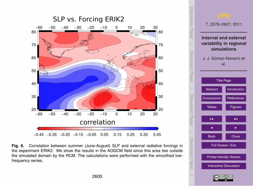
CPD7, 2579–2607, 2011


simulations


Title Page



Tables Figures

J I

J I

Back Close

Full Screen / Esc



Discussion

Paper

|D

iscussionP

aper|

Discussion

Paper

|D

iscussionP

aper|


-2

0

2

4

1000 1100 1200 1300 1400 1500 1600 1700 1800 1900 2000

−1.8

−1.4−1−0.6

−0.20.2

−1.8 −1.4 −1.0 −0.6 −0.2 0.2 0.6 1.0 1.4 1.8

1

1

1

0.5 0.6 0.7 0.8 0.9 1.0 1.1 1.2 1.3

−0.7

−0.7

−0.5

−0.3 −0.1

−0.1

0.10.10.3

−0.9 −0.7 −0.5 −0.3 −0.1 0.1 0.3 0.5 0.7 0.9

PC1 PRE ERIK1PC1 PRE ERIK2

PC1 SAT ERIK1PC1 SAT ERIK2

Forcing

EOF1 SAT EOF1 PRE CORR SAT-PRE

a) b) c)

d)

MM5-ERIK2 summer

Fig. 5. Evolution of the summer (June-August) SAT and PRE dur-ing the last millennium in the two simulations. The three top mapsshow the first EOF of the standardised SAT (Fig. a) and PRE (Fig.b), as well as the correlation between these two variables (Fig. c).All maps are dimensionless, and correspond to the MM5-ERIK2 ex-periment, since the corresponding maps for MM5-ERIK1 are verysimilar (not shown). Fig. d shows the normalised PCs associatedwith the two variables in the two experiments, as well as the ex-ternal radiative forcing. All calculations were performed with thesmoothed low-frequency series.

relation between the PCs, as well as the high percentage ofvariance that the first EOF for each variable explains, drivethe clear correlation between these variables and their spatialstructure.

On the other hand, the correlations between the PCs of thetwo experiments are 0.81 and 0.34 for SAT and PRE, respec-tively. This is in good agreement with our previous finding ofa stronger influence of the external forcings in the evolutionof SAT than in the case of PRE. In addition, the similaritybetween the map in Figure 5c (or Figure 5b) and correlationmaps in Figure 3 for summer is clear. Again, the explanationfor the structure and intensity of these correlation patterns isbetter sought in the EOF analysis. The homogeneous firstEOF, together with the large amount of variability it explainsand the large correlation between the associated PCs, forcea high and homogeneous correlation between the SAT in thetwo experiments. On the contrary, the lower correlation be-tween PCs associated with the evolution of PRE in the twoexperiments precludes strong coupling between them. De-spite this, the shape of the main variability mode is similarin the two simulations, and the correlation between both PCsis not negligible, which explains why the areas most affectedby this pattern stand out in the correlation maps of Figure 3.

Having identified that the response to the forcing in sum-mer precipitation over the IP is due to the main variabilitymode, which has the same spatial structure and is clearly cor-related in the two simulations, we sought the physical mech-

−60

−60

−50

−50

−40

−40

−30

−30

−20

−20

−10

−10

0

0

10

10

20

20

30

30

20 20

30 30

40 40

50 50

60 60

70 70

80 80

−0.45 −0.35 −0.25 −0.15 −0.05 0.05 0.15 0.25 0.35 0.45

SLP vs. Forcing ERIK2

correlation

Fig. 6. Correlation between summer (June-August) SLP and ex-ternal radiative forcings in the experiment ERIK2. We show theresults in the AOGCM field since this area lies outside the simu-lated domain by the RCM. The calculations were performed withthe smoothed low-frequency series.

anism behind this link. First, we separately considered large-scale and convective precipitation. The correlation mapsequivalent to those shown in Figure 3 for convective precipi-tation alone, depict very low values and no spatial structure,whereas the maps corresponding to large-scale precipitationlook very similar to those in Figure 3 (not shown). This sug-gests that the response to forcing is in the large-scale field, inparticular in the response of regional circulation to externalforcings. To confirm this, Figure 6 shows the correlation be-tween the low-frequency filtered series of external forcingsand SLP for summer in the ERIK2 experiment (the map cor-responding to ERIK1, not shown, exhibits the same patternand supports the same physical explanation). We show thecalculations in the AOGCM fields since this area lies out-side the domain simulated by the RCM, and, in any case, thedifferences between the RCM and the AOGCM in the SLPfield are small. This figure shows how the local circulation isaffected by the driving forcings. In particular the strengthen-ing of the Azores high reduces the large-scale precipitationover the northwest, whereas the low over Morocco has theopposite effect and is responsible for the simultaneous in-crease of precipitation in the southeast of the IP and over theMediterranean Sea, which is precisely the shape of the firstEOF shown in Figure 5b.

The results for winter are different. As discussed above,Figure 3 shows how the correlation structure for winter isdifferent from that of summer, which suggests that the un-derlying physical mechanism may also be different. Figures7a, b and c are equivalent to Figures 5a, b and c for winter (as

Fig. 6. Correlation between summer (June-August) SLP and external radiative forcings inthe experiment ERIK2. We show the results in the AOGCM field since this area lies outsidethe simulated domain by the RCM. The calculations were performed with the smoothed low-frequency series.

2605





CPD7, 2579–2607, 2011


simulations


Title Page



Tables Figures

J I

J I

Back Close

Full Screen / Esc



Discussion

Paper

|D

iscussionP

aper|

Discussion

Paper

|D

iscussionP

aper|

J.J. Gomez-Navarro et al.: Internal and external variability in regional simulations 7

−2.7 −2.1 −1.5 −0.9 −0.3 0.3 0.9 1.5 2.1 2.7

0.80.8

0.9

0.9

0.90.9

0.9

1

1

1.1

1.2

1.3

0.5 0.6 0.7 0.8 0.9 1.0 1.1 1.2 1.3

−1.4

−1.4

−1.4

−1−1

−0.6

−0.6

−0.2−0.2

−1.8 −1.4 −1.0 −0.6 −0.2 0.2 0.6 1.0 1.4 1.8

−0.5

−0.5

−0.3

−0.3

−0.3

−0.1

−0.1

−0.10.1

0.1

0.3

−0.9 −0.7 −0.5 −0.3 −0.1 0.1 0.3 0.5 0.7 0.9

−0.7

−0.5

−0.5−0.3

−0.3

−0.1

−0.1−0.1

−0.9 −0.7 −0.5 −0.3 −0.1 0.1 0.3 0.5 0.7 0.9

EOF1 SAT EOF1 PRE

CORR PRE-NAO

CORR SAT-PRE

EOF2 PRE

MM5-ERIK2 winter

a) b) c)

−1.5

−0.9

−0.9

−0.3

−0.3

0.3 0.3

0.3

0.9

0.9

e)d)

Fig. 7. The three top maps show the first EOF of standardised seriesof winter SAT (Fig. a) and PRE (Fig. b), as well as the correlationbetween these two variables (Fig. c). Fig. d shows the correlationbetween the precipitation series and the NAO index, defined as thePC associated with the leading EOF of SLP in the North Atlanticarea. Fig. e is the first EOF of the winter residual precipitation, oncethe NAO signal has been removed, following the methodology de-tailed in the main text. All maps are dimensionless and correspondto the MM5-ERIK2 experiment, since the corresponding maps forMM5-ERIK1 are analogous (not shown). The calculations wereperformed with the smoothed low-frequency series.

before, the following argument is based on the MM5-ERIK2experiment, although it also holds for the MM5-ERIK1 ex-periment). The evolution of SAT in winter is dominated bya homogeneous EOF, with associated PCs that are stronglycorrelated in the two experiments (correlation 0.68). How-ever an important difference between summer and winter isthat in the latter, the leading EOF for precipitation (Fig. 7b)is very different from the correlation pattern between tem-perature and precipitation (Fig. 7c). The explanation forthis difference has to be sought in the impact of large-scalecirculation in the precipitation regime in winter over the IP.The North Atlantic Oscillation (NAO) is a variability modeof SLP in the North Atlantic area which strongly affects thewinter precipitation amount in the IP, especially in the west-ern parts (Trigo et al., 2004). The MM5-ECHO-G model isable to successfully reproduce this feature (Gomez-Navarroet al., 2011). Figure 7d illustrates this by showing the corre-lation between the NAO index, defined as the PC associatedto the first EOF of winter SLP in the North Atlantic area, andthe PRE series in each grid point. It is apparent how the areasmost affected by NAO (Fig. 7d) are those standing out in thefirst EOF of PRE (Fig. 7b). This means that in winter themain variability mode of precipitation is dominated by NAOvariations. However, the correlation of the low-frequencyvariations of NAO in the two simulations is only 0.17 (be-

low 0.27, the significance level at the 95% confidence level),indicating that this important circulation mode does not re-spond to the external forcing, but is dominated by internalvariability in the AOGCM. This explains the generally lowerimpact of the driving forcing in the evolution of precipitationin winter. In winter, the fingerprint of the relationship be-tween SAT and PRE illustrated in Figure 7c has to be soughtin the second EOF. This is shown in Figure 7e and explains18% of the low-frequency precipitation variance, once theNAO signal has been removed by the first EOF. We comparethis second most important variability mode for winter pre-cipitation with the correlation pattern between SAT and PRE.This mode of precipitation variability, once the influence ofthe non-forced NAO has been removed, responds to the forc-ings, as can be identified by comparing Figure 7e and the cor-relation maps for winter in Figure 3. In fact, the correlationbetween the PC associated to this precipitation mode and thePC associated with the SAT is 0.62 (0.66 in MM5-ERIK1).

The physical link between temperature and precipitationin winter described above, which is responsible for the re-semblance between the evolution of the precipitation seriesduring this season in the two simulations shown in Fig. 3, isnot due to the response of the large-scale circulation to theexternal forcings, as the case of summer. Instead, it is due tothe interactions between the large-scale circulation and theorography of the RCM. Fig. 8a shows the correlation be-tween the low-frequency evolution of precipitation series inthe two simulations, together with the orography consideredby the model (in green contours). The correlation is moreintense near the main mountain systems such as the northside of the Pyrenees or the western part of the Iberian andBetic systems. This figure, together with the characteristicanti-correlation map between temperature and precipitationshown in Fig. 7c, suggests that may exist a modulation in thecondensation level, driven by temperature variations, whichwould could affect specially the precipitation over moun-tanous regions. To check this, the condensation level has tobe calculated within the simulations. This variable can be re-lated with the dew point temperature in good approximationby the difference:

CL∝ (T −Td) (3)

where T is temperature and Td is the dew point temperature,both variables measured in the surface (Lawrence (2005)presents a modern review on the relations between moisture,temperature and how they are related). Fig. 8b shows the cor-relation between temperature variations and the temperaturedifferences in Eq. 3. There is a generally strong and positiverelation between the height of the condensation level and thetemperature (which is not an obvious result since the mois-ture content over the IP depends to a large extent on the evap-oration rate in the Atlantic Ocean, which is lower in colderperiods). The relation is stronger near the main mountainsystems, although the correlation map also depict sensitiv-ity to the Atlantic flow on the windward side of the moun-

Fig. 7. The three top maps show the first EOF of standardised series of winter SAT (a) andPRE (b), as well as the correlation between these two variables (c). (d) shows the correlationbetween the precipitation series and the NAO index, defined as the PC associated with theleading EOF of SLP in the North Atlantic area. (e) is the first EOF of the winter residualprecipitation, once the NAO signal has been removed, following the methodology detailed inthe main text. All maps are dimensionless and correspond to the MM5-ERIK2 experiment,since the corresponding maps for MM5-ERIK1 are analogous (not shown). The calculationswere performed with the smoothed low-frequency series.

2606





CPD7, 2579–2607, 2011


simulations


Title Page



Tables Figures

J I

J I

Back Close

Full Screen / Esc



Discussion

Paper

|D

iscussionP

aper|

Discussion

Paper

|D

iscussionP

aper|


−0.9 −0.7 −0.5 −0.3 −0.1 0.1 0.3 0.5 0.7 0.9

correlation

Corr PRE-PRE Corr SAT-CL

a) b)

Fig. 8. Physical response of winter precipitation over the IP. Fig.a) shows the correlation between precipitation series in the MM5-ERIK1 and MM5-ERIK2 experiments, and it is the analog to Figure3 but using a low-pass filter instead of running means. Fig. b) de-picts the correlation between the temperature and height of the con-densation level in the MM5-ERIK2 experiment. All calculationswere performed using the low-frequency series. Green contours in-dicate the terrain height above 500 metres spaced by 300 metres.

tains. That is, in cold periods the condensation level sinks,especially on the windward side of the mountains, and thisflavours the increase of precipitation in these areas. Hence,the physical link between precipitation and forcing in winteris through variations in the condensation level, directly mod-ulated by variations in temperature. Surprisingly, despite theintensity of the noise due to internal variability in the winterprecipitation, this mechanism is strong enough to leave anobservable mark in the amount of precipitation in some areasover the IP, characterised by the orography. It is important tonote that this mechanism can only be accurately reproducedwithin the context of a high resolution simulation capable ofresolving the fine spatial scales involved.

4 Summary and Conclusions

In this study we have compared the evolution of SAT andPRE in two millennial paleoclimate simulations performedwith a RCM with a spatial resolution of 30 km for the IP. Thecomparison allows us to evaluate the importance and magni-tude of the internal variability in the evolution of these vari-ables, compared with the influence of the reconstruction ofexternal forcings used to drive the simulations. The under-lying argument is that if external forcings play a weak rolein the evolution of the simulation, the temporal correlationof the series associated with these variables in both simula-tions should not be also weak, since the internal variability,generated by the chaotic nature of the climatic system, is un-correlated in both simulations.

The results indicate that the long-term evolution of SAT isstrongly affected by the the external forcings driving the sim-ulation. This variable responds homogeneously to the exter-nal factors over the IP at most temporal scales. The evolutionof PRE is, however, more strongly governed by chaotic vari-ability at regional scale. In particular, there are few areasin the IP, the main mountain system in winter and the Northand West areas in summer, where the precipitation is signif-icantly driven by external forcings. However, in many partsof the domain the influence of the external forcing can notbe detected in the evolution of PRE. It is important to notethat the significance of the correlation emerges at regionalscales, and is blurred when a spatial average is performed.This stresses the importance of high resolution simulationsin exercises comparing the model results with proxy recon-structions of precipitation.

The influence of the external forcing on precipitation is es-pecially weak in winter. This is due to the nature of the winterprecipitation over the IP, which is dominated by variations inthe NAO. The NAO seems to be quite insensitive to the exter-nal forcing in the simulations at the investigated timescales.Once the NAO signal is removed from the precipitation se-ries, the leading variability pattern corresponds quite wellwith the areas which are more clearly able to respond to forc-ings. Precipitation in summer is more strongly affected byvariations in the forcing. Its main variability mode matcheswell the areas where summer precipitation responds to exter-nal forcing. In fact, we have been able to demonstrate thatthis precipitation mode is dominated by modulation of thelarge-scale SLP by the external forcing in summer. This isin contrast with the stronger contribution of the internal vari-ability of SLP in winter. During this season, there are stillsome areas where precipitation responds the the forcing, but,in this case, it is not through modification in the large-scaleflow, but through the interaction between condensation leveland orography.

Our findings regarding the impact of internal variability inthe simulations may have a strong impact on how compari-son between simulations and reconstructions are performed.In particular, we have been able to identify areas where weshould not expect good agreement between the model andthe reconstructions, even if both are perfect. On the otherhand, there are areas, mostly in the main mountain systems,where mismatches between both approaches can not be ar-gued to be due to internal variability. These results stressthe importante of RCMs in paleoclimate studies, since wehave demonstrated that the physical mechanism responsiblefor the response of precipitation to external forcings in wintercan only be realistically reproduced by using high resolutionsimulations.

A further important comment has to be made regardingthe reconstructions of solar forcing used in these simula-tions. The evolution of the TSI used in these simulationsis taken from Crowley (2000). However, a more recent re-construction of this variable (Krivova and Solanki, 2008) de-

Fig. 8. Physical response of winter precipitation over the IP. (a) shows the correlation betweenprecipitation series in the MM5-ERIK1 and MM5-ERIK2 experiments, and it is the analog toFig. 3 but using a low-pass filter instead of running means. (b) depicts the correlation betweenthe temperature and height of the condensation level in the MM5-ERIK2 experiment. All cal-culations were performed using the low-frequency series. Green contours indicate the terrainheight above 500 metres spaced by 300 m.

2607





Documents

Internal and external variability in regional simulationsdigital.csic.es/bitstream/10261/62232/1/CPD_2011_7_2579.pdf · Internal and external variability in regional simulations