Embed Size (px)
Citation preview

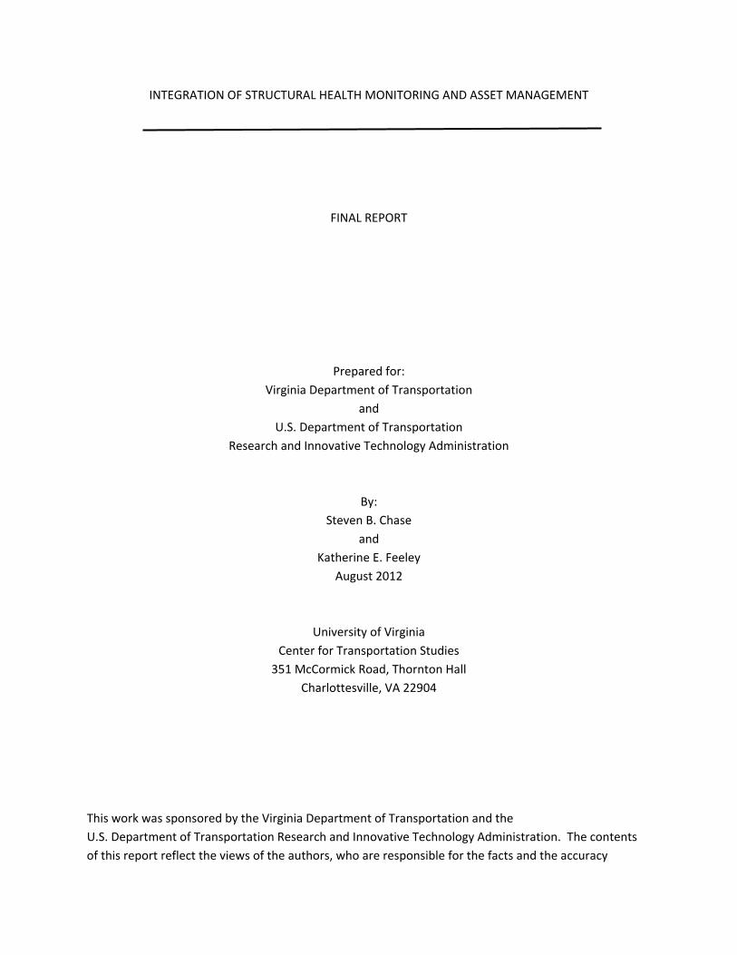
Integration of Structural Health Monitoring and Asset Management
Prepared by
University of Virginia
The Pennsylvania State University University of Maryland University of Virginia Virginia Polytechnic Institute and State
University West Virginia University
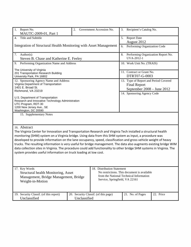
INTEGRATION OF STRUCTURAL HEALTH MONITORING AND ASSET MANAGEMENT
FINAL REPORT
Prepared for: Virginia Department of Transportation
and U.S. Department of Transportation
Research and Innovative Technology Administration
By: Steven B. Chase
and Katherine E. Feeley
August 2012
University of Virginia Center for Transportation Studies
351 McCormick Road, Thornton Hall Charlottesville, VA 22904
This work was sponsored by the Virginia Department of Transportation and the U.S. Department of Transportation Research and Innovative Technology Administration. The contents of this report reflect the views of the authors, who are responsible for the facts and the accuracy


ABSTRACT
This project investigated the feasibility and potential benefits of the integration of infrastructure monitoring systems into enterprise-scale transportation management systems. An infrastructure monitoring system designed for bridges was implemented and a framework was developed for the integration of bridge-level data into the distributed network-level asset condition and performance data already existing within VDOT’s bridge asset management system.
It is now fairly common to install sensors in highway infrastructure to assess and monitor the performance and health of pavements and bridges. [Add references] A companion report prepared by Virginia tech documents the use of sensors in pavements to provide data useful for pavement management. The University of Virginia project focused on studying how to use a bridge structural health monitoring system (SHM) installed for structural monitoring purposes, to support bridge management.
A structural health monitoring system was installed on a Virginia bridge as part of a separate project sponsored under the Long Term Bridge Performance Program. That SHM system was designed and installed to provide data on the structural performance and response of the bridge to ambient loading and to support periodic load tests. The primary objectives were to demonstrate the state of the art in SHM technology, to serve as a test bed for the development of load testing protocols and to document changes in bridge behavior as the bridge continued to age. A number of sensors were strategically located and installed on the bridge, a permanent data acquisition system was installed with the ability to continuously monitor the sensors, a communications system was installed to provide for remote access for data collection and control of the system and a companion video camera capable of providing streaming video images of the traffic on the bridge was installed. The total system represented a significant investment.
This study, completed by the University of Virginia (UVA), investigated and developed a procedure to use select data from the SHM system and to provide information that is useful for bridge management purposes. UVA focused on providing data on heavy vehicles. The response of highway bridges to passenger vehicles is very small and insignificant when considering fatigue or overloads. The significant live loading of highway bridges is due to trucks. A simple and relatively inexpensive system to measure and monitor the truck loading on specific highway bridges would be a useful tool for bridge management. The current practice is to estimate truck volumes as a percentage of average daily traffic. This provides an estimate of truck volume but does not provide any information on the magnitude and frequency of the loading due to heavy trucks. It also does not provide any information on which lanes are loaded. If such information could be provided, it would be very useful in assessing the fatigue loading of a bridge and also assess the frequency and severity of overload events. The procedure reported here provides such information.

The specific tasks completed by UVA were:
1) Develop of a finite element model (FEM) of the bridge using the SAP 2000 software. 2) Calibrate the FEM using data from the initial load testing of the bridge performed by Virginia
tech. 3) Use the calibrated FEM to create moment and strain influence surfaces for arbitrary point loads
on the bridge. 4) Use the influence surfaces to simulate the effect of trucks of arbitrary axle configurations and
gross vehicle weights travelling over the bridge in different lanes and at different speeds at all of the selected sensors.
5) Use the simulation program to generate hundreds of simulated truck events to create a response database.
6) Use the response database to develop a procedure to determine: a. The travel lane of the truck, b. The speed of the truck, c. The vehicle class of the truck (a 3 axle single unit or a 5 axle semi- tractor trailer), and d. The gross vehicle weight of the truck
7) Test the procedure on actual truck events.
A straightforward and easily implementable procedure was developed to use data from a typical bridge structural health monitoring system to provide lane occupancy, speed, vehicle classification and gross vehicle weight estimates for heavy trucks.
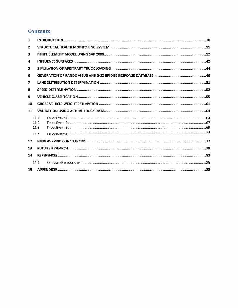
1. Report No.
MAUTC-2009-01, Part 1 2. Government Accession No.
3. Recipient’s Catalog No.
4. Title and Subtitle Integration of Structural Health Monitoring with Asset Management
5. Report Date August 2012
6. Performing Organization Code
7. Author(s) Steven B. Chase and Katherine E. Feeley
8. Performing Organization Report No. UVA-2012-1
9. Performing Organization Name and Address The University of Virginia 201 Transportation Research Building University Park, PA 16802
10. Work Unit No. (TRAIS)
11. Contract or Grant No. DTRT07-G-0003
12. Sponsoring Agency Name and Address Virginia Department of Transportation 1401 E. Broad St. Richmond, VA 23219 U.S. Department of Transportation Research and Innovative Technology Administration UTC Program, RDT-30 1200 New Jersey Ave., SE Washington, DC 20590
13. Type of Report and Period Covered Final Report September 2008 – June 2012 14. Sponsoring Agency Code
15. Supplementary Notes
16. Abstract The Virginia Center for Innovation and Transportation Research and Virginia Tech installed a structural health monitoring (SHM) system on a Virginia bridge. Using data from this SHM system as input, a procedure was developed to provide information on the lane occupancy, speed, classification and gross vehicle weight of heavy trucks. The resulting information is very useful for bridge management. The data also augments existing bridge WIM data collection sites in Virginia. The procedure could add functionality to other bridge SHM systems in Virginia. The system provides useful information on truck loading at low cost.
17. Key Words
Structural health Monitoring, Asset Management, Bridge Management, Bridge Weight-in-Motion
18. Distribution Statement No restrictions. This document is available from the National Technical Information Service, Springfield, VA 22161
19. Security Classif. (of this report) Unclassified
20. Security Classif. (of this page) Unclassified
21. No. of Pages
22. Price
Contents 1 INTRODUCTION ........................................................................................................................................ 10
2 STRUCTURAL HEALTH MONITORING SYSTEM ........................................................................................... 11
3 FINITE ELEMENT MODEL USING SAP 2000 ................................................................................................. 12
4 INFLUENCE SURFACES .............................................................................................................................. 42
5 SIMULATION OF ARBITRARY TRUCK LOADING .......................................................................................... 44
6 GENERATION OF RANDOM SU3 AND 3-S2 BRIDGE RESPONSE DATABASE .................................................. 46
7 LANE DISTRIBUTION DETERMINATION ..................................................................................................... 51
8 SPEED DETERMINATION ........................................................................................................................... 52
9 VEHICLE CLASSIFICATION .......................................................................................................................... 55
10 GROSS VEHICLE WEIGHT ESTIMATION ...................................................................................................... 61
11 VALIDATION USING ACTUAL TRUCK DATA ................................................................................................ 64
11.1 TRUCK EVENT 1 ............................................................................................................................................. 64 11.2 TRUCK EVENT 2 ............................................................................................................................................. 67 11.3 TRUCK EVENT 3 ............................................................................................................................................. 69 11.4 TRUCK EVENT 4 ............................................................................................................................................. 73
12 FINDINGS AND CONCLUSIONS .................................................................................................................. 77
13 FUTURE RESEARCH ................................................................................................................................... 78
14 REFERENCES ............................................................................................................................................. 82
14.1 EXTENDED BIBLIOGRAPHY ............................................................................................................................... 85
15 APPENDICES ............................................................................................................................................. 88

List of Figures Figure 1 SHM Layout Diagram .................................................................................................... 13 Figure 2 Cross Section A-A .......................................................................................................... 13 Figure 3 Cross Section B-B .......................................................................................................... 14 Figure 4 Cross Section C-C .......................................................................................................... 14 Figure 5 Cross Section D-D .......................................................................................................... 14 Figure 6 Cross Section E-E ........................................................................................................... 15 Figure 7 Photograph of Route 15 Bridge (Courtesy of Virginia Tech) ....................................... 15 Figure 8 Satellite Image of Route 15 Bridge (Courtesy of Google Maps) ................................... 15 Figure 9 SAP-2000 Bridge Wizard (New Model) ........................................................................ 16 Figure 10 Span Definition Menu .................................................................................................. 16 Figure 11 Bridge Modeler Menu .................................................................................................. 17 Figure 12Bridge Materials Menu .................................................................................................. 17 Figure 13 Frame Properties Menu ................................................................................................ 18 Figure 14 Section Definition menu ............................................................................................... 18 Figure 15 I/Wide Flange Definition Menu ................................................................................... 18 Figure 16 Non-Prismatic Menu .................................................................................................... 19 Figure 17 Non-prismatic Definition Menu ................................................................................... 20 Figure 18 Deck Section Definition Menu ..................................................................................... 20 Figure 19 Define Deck Section Data Menu .................................................................................. 21 Figure 20 Diaphragm Definition Menu ........................................................................................ 22 Figure 21 Diaphragm Properties Menu......................................................................................... 22 Figure 22 Bridge Object Definition Menu .................................................................................... 23 Figure 23 Bridge Object Data Menu ............................................................................................. 23 Figure 24 Bridge Span Section Definition Menu ......................................................................... 24 Figure 25 Bridge Abutment Definition Menu .............................................................................. 25 Figure 26 Bent Definition Menu ................................................................................................... 26 Figure 27 Bent Data Assignment Menu........................................................................................ 27 Figure 28Cross Diaphragm Assignment Menu............................................................................. 28 Figure 29 Bridge Object Plan View .............................................................................................. 28 Figure 30Bridge Model Update Menu .......................................................................................... 29 Figure 31 Spline Model ................................................................................................................ 30 Figure 32 Spline Area Model ........................................................................................................ 31 Figure 33 Full Area Model ........................................................................................................... 31 Figure 34 Lane Definition Menu .................................................................................................. 32 Figure 35 Lane Data Menu ........................................................................................................... 33 Figure 36 Lane Data Menu (2) ...................................................................................................... 33 Figure 37 Vehicle Definition Menu .............................................................................................. 34 Figure 38 Vehicle Data Menu ....................................................................................................... 34 Figure 39 General Vehicle Data Menu ......................................................................................... 35 Figure 40 Vehicle Class Definition Menu .................................................................................... 35 Figure 41 Vehicle Class Data Menu ............................................................................................. 36 Figure 42 Moving Load Results Selection Menu ......................................................................... 36 Figure 43 Load Pattern Definition Menu ...................................................................................... 37 Figure 44 Multi-step Live Load Pattern Generation Menu .......................................................... 37
Figure 45 Load Case Definition Menu ......................................................................................... 38 Figure 46 Load Case Data Menu .................................................................................................. 38 Figure 47 Moving Load Data Menu ............................................................................................. 39 Figure 48 Deflected Shape View .................................................................................................. 40 Figure 49 Moment Envelope for Entire Bridge Section ............................................................... 41 Figure 50 Influence Line/Surface Definition Menu ...................................................................... 41 Figure 51 Influence Surface for SG3N ......................................................................................... 42 Figure 52 Influence Surface for SG3S .......................................................................................... 43 Figure 53 Influence Surface for SG5N ......................................................................................... 43 Figure 54 Influence Surface for SG5S .......................................................................................... 44 Figure 55 Beam Model for Influence Line ................................................................................... 44 Figure 56 Moment Influence Lines for Sensors 1 and 2 ............................................................... 45 Figure 57 AASHTO HS-20 Design Vehicle ................................................................................. 45 Figure 58 Response at Sensor 1 for HS-20 Vehicle Passing Over Beam ..................................... 45 Figure 59 Definition of SU3 Truck ............................................................................................... 47 Figure 60 Response of SG3N to SU3 Truck at Different Speeds ................................................. 48 Figure 61 Response of SG3N to 10 Random SU3 Trucks ............................................................ 49 Figure 62 Definition of 3-S2 Truck .............................................................................................. 49 Figure 63 Response of Sensor SG5S to 10 random 3-S2 Trucks ................................................. 50 Figure 64 Trace of All Four Sensors to a SU3 Truck .................................................................. 51 Figure 65 Response of all Four Sensors to a 3-S2 Truck ............................................................. 51 Figure 66 SG3N/SG5N Ratios for Lane 1 and 2 .......................................................................... 52 Figure 67 Lane Occupancy Determination ................................................................................... 53 Figure 68 Traces for 3-S2 Vehicle at 20 MPH ............................................................................. 54 Figure 69 Traces for SU3 Vehicle at 60 MPH .............................................................................. 54 Figure 70 Response Traces for SU3 Truck in Lane 1 ................................................................... 55 Figure 71 Response Traces for SU3 in Lane 2 ............................................................................. 56 Figure 72 Response Traces for 3-S2 Truck in Lane 1 .................................................................. 56 Figure 73 Response Traces for 3-S2 in Lane 2 ............................................................................. 57 Figure 74 Empirically Determined Classification Feature Vector ............................................... 57 Figure 75 50 Random Feature Vectors for SU3 and 3-S2 Vehicles ............................................. 58 Figure 76 Feature Vector for SU3 Vehicle ................................................................................... 59 Figure 77 Feature Vector for 3-S2 Vehicle ................................................................................... 59 Figure 78 Schematic of Feed Forward Neural Network ............................................................... 60 Figure 79 Confusion Matrix for Neural Network ......................................................................... 60 Figure 80 Relation Between Peak Positive Strain and GVW ....................................................... 61 Figure 81 Relationship Between Minimum Strain and GVW, SU3 in Lane 1 ............................. 62 Figure 82 Relationship Between Minimum Strain and GVW, SU3 in Lane 2 ............................. 62 Figure 83 Relationship Between Minimum Strain and GVW, 3-S2 in Lane 1 ............................ 63 Figure 84 Relationship Between Minimum Strain and GVW, 3-S2 in Lane 2 ............................ 63 Figure 85 Raw Data for Truck #1 ................................................................................................. 64 Figure 86 Filtered Data for Truck #1 ............................................................................................ 65 Figure 87 Feature Vector for Truck #1 ......................................................................................... 66 Figure 88 Neural Network Classification for Truck #1 ................................................................ 67 Figure 89 Filtered Data for Truck #2 ............................................................................................ 67 Figure 90 Feature Vector for Truck #2 ......................................................................................... 68

Figure 91 Neural Network Classification for Truck #2 ................................................................ 69 Figure 92 Filtered Data for Truck #3 ............................................................................................ 70 Figure 93 Time Series Data for Truck #3 ..................................................................................... 71 Figure 94 Feature Vector for Truck #3 ......................................................................................... 72 Figure 95 Neural Network Classification of Truck #3 ................................................................. 72 Figure 96 Filtered Data for Truck #4 ............................................................................................ 73 Figure 97 Time Series Data for Truck # 4 .................................................................................... 74 Figure 98 Feature Vector for Truck #4 ......................................................................................... 75 Figure 99 Filtered Data for 10,000 Samples ................................................................................. 76 Figure 100 Dynamic Amplification for the Bridge....................................................................... 77 Figure 101Trace with Multiple Vehicles ...................................................................................... 79 Figure 102 FHWA Vehicle Classifications .................................................................................. 80
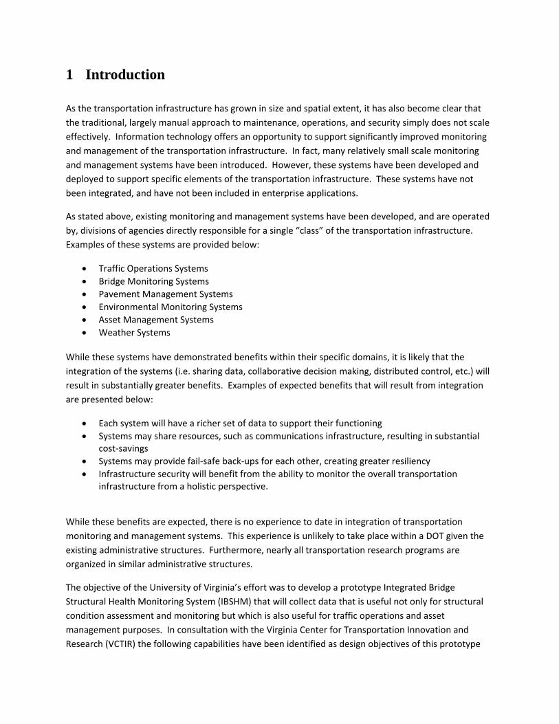
1 Introduction
As the transportation infrastructure has grown in size and spatial extent, it has also become clear that the traditional, largely manual approach to maintenance, operations, and security simply does not scale effectively. Information technology offers an opportunity to support significantly improved monitoring and management of the transportation infrastructure. In fact, many relatively small scale monitoring and management systems have been introduced. However, these systems have been developed and deployed to support specific elements of the transportation infrastructure. These systems have not been integrated, and have not been included in enterprise applications.
As stated above, existing monitoring and management systems have been developed, and are operated by, divisions of agencies directly responsible for a single “class” of the transportation infrastructure. Examples of these systems are provided below:
• Traffic Operations Systems • Bridge Monitoring Systems • Pavement Management Systems • Environmental Monitoring Systems • Asset Management Systems • Weather Systems
While these systems have demonstrated benefits within their specific domains, it is likely that the integration of the systems (i.e. sharing data, collaborative decision making, distributed control, etc.) will result in substantially greater benefits. Examples of expected benefits that will result from integration are presented below:
• Each system will have a richer set of data to support their functioning • Systems may share resources, such as communications infrastructure, resulting in substantial
cost-savings • Systems may provide fail-safe back-ups for each other, creating greater resiliency • Infrastructure security will benefit from the ability to monitor the overall transportation
infrastructure from a holistic perspective.
While these benefits are expected, there is no experience to date in integration of transportation monitoring and management systems. This experience is unlikely to take place within a DOT given the existing administrative structures. Furthermore, nearly all transportation research programs are organized in similar administrative structures.
The objective of the University of Virginia’s effort was to develop a prototype Integrated Bridge Structural Health Monitoring System (IBSHM) that will collect data that is useful not only for structural condition assessment and monitoring but which is also useful for traffic operations and asset management purposes. In consultation with the Virginia Center for Transportation Innovation and Research (VCTIR) the following capabilities have been identified as design objectives of this prototype

bridge monitoring system. The system will monitor the structural response of a highway bridge to ambient traffic and provide the following structural health data: (1) stress/strain histories at selected locations on the bridge suitable for estimation of the cumulative fatigue loading of the bridge, (2) the system will provide data that measures and characterizes the occurrence of large load events (i.e., overloads), (3) the system will provide data that can be used to characterize the dynamic amplification factor of the bridge, and (4) the system will provide the capability of measuring and characterizing the response of the bridge to static loads, suitable for periodic load testing and rating of the bridge. In order to operate reliably over a long period, the structural health monitoring system must necessarily compensate for any system drift. Consequently, the system must measure and compensate for the effects of temperature and humidity. Finally, in addition to the structural health and environmental data, the system will also be designed to operate as (5) a bridge based weigh-in-motion (WIM) station. As such, the system will provide quantitative data on the number, classification and total weight of heavy trucks that pass over the bridge.
2 Structural Health Monitoring System
A project sponsored under the FHWA’s Long Term Bridge Performance Program was the installation of a long term structural health monitoring (SHM) system on the bridge that carries Route 15 over Interstate 66 in Haymarket, Virginia. The SHM system is to monitor the bridge’s response to ambient traffic and environmental loadings and support periodic load testing using heavy trucks of known weight and configuration. The SHM system consisted of a network of sensors, a computerized data acquisition and data logging system, remote communications capability and a video streaming system to provide images of the traffic on the bridge. The SHM system is only one aspect of a complete health assessment of the bridge. In addition to the SHM system, detailed hands-on visual inspection, materials sampling and testing and extensive nondestructive evaluation of the bridge is also being performed.
While very sophisticated and expensive, the SHM system was not designed to provide information for asset management uses. The data being obtained could be used for that purpose by expert interpretation but that is not being done at this time. The University of Virginia project being reported processed data from a select number of the sensors to provide information more useful from a bridge asset management perspective. Specifically data from four of the eight strain gages installed on the bridge were used as input to a processing algorithm to extract lane occupancy, vehicle speed, vehicle classification and gross vehicle weight of heavy trucks. A brief description of the SHM system is provided as a reference to the sensors that were used as inputs to the algorithm.
The Virginia Bridge has a total of 22 long-term sensors installed. The sensors employed are linear variable differential transformers (LVDTs), bonded foil strain gauges, vibrating wire strain gauges, and thermocouples. Error! Reference source not found.through Error! Reference source not found. show the location of each of the structural sensors on plan and cross-sectional views of the bridge.
The four sensors used for processing are the bonded foil strain gages located on the top of the bottom flange in Girders 3 and 5 at cross sections AA and CC. These sensors are designated as SG3N, SG3S, SG5N

and SG5S. The SG refers to the fact that these are strain gages, the number refers to the girder and the S and N refer to South and North spans respectively. This bridge is one of a pair of parallel bridges carrying Route 15 over Interstate 66. This is the southbound bridge and all traffic moves from North to South on the bridge.
3 Finite Element Model using SAP 2000
Finite element methods are extremely useful for the analysis and design of complex structures. There are many different commercial and academic software systems that implement the finite element method within a framework for the solution of a wide variety of problems in different domains. Some general purpose systems, such as ANSYS and ABAQUS, are designed to be applied to a wide range of problems and are consequently very sophisticated. However, they require significant effort to apply to the simulation of highway bridges. Other software is designed to be applied to specific domains. One such system is SAP-2000, which is focused on the analysis and design of structures. In particular, SAP-2000 includes many features specifically designed to facilitate the modeling and analysis of highway bridges. These features include a wizard to quickly define the overall geometry and basic structure of a bridge, material libraries and multiple element types suitable for bridges, a range of modeling options from very simple beam models to complex 3-D plate and shell models, and built in tools to greatly facilitate the modeling of loading due to moving vehicles of arbitrary dimensions. In addition, SAP-2000 provides the ability to import and export model inputs and outputs to a variety of formats, including el worksheets. SAP-2000 was used to model the response of the Route 15 bridge to vehicle loads and to generate influence surfaces of sensor responses that were then used for general simulation of bridge response to random loads.
A detailed description of the modeling of the Route 15 bridge using SAP-2000 is contained in Feely 2010. A summary of the modeling with particular emphasis on the generation of influence surfaces is presented in this report.
On a separate project sponsored by the FHWA’s Long Term Bridge Performance Program, the southbound lane of the Haymarket (Route 15) Bridge was selected for installation of a Structural Health Monitoring (SHM) system. The Route 15 Bridge is a two-span continuous bridge with a non-uniform cross section. It is located in Haymarket, Virginia at the intersection of Interstate 66 and Virginia Route 15. Refer to Figure 7 and 8 for a photograph of the bridge and the satellite image of the bridge and its surrounding area.. The Route 15 Bridge has a skew of nearly 17.5 degrees and has six steel girders, re composed of built-up plate sections. The bridge has an 8.5 inch composite concrete deck with top girder flanges embedded into a 3 inch haunch. In-span cross V-diaphragms occur along the span of the bridge every 22’-8”. Lateral bracing occurs between the fascia girders and the immediate interior girders. All bridge dimensions were taken from the plan provided by the Virginia department of Transportation.
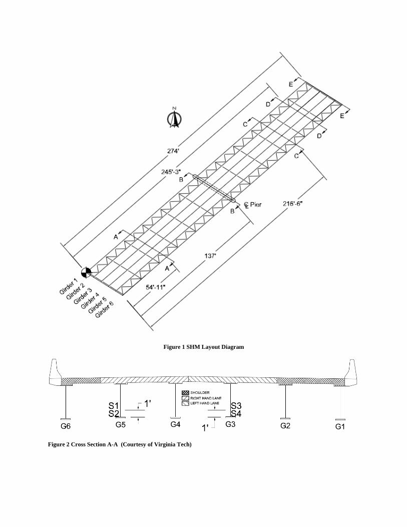
Figure 1 SHM Layout Diagram
Figure 2 Cross Section A-A (Courtesy of Virginia Tech)

Figure 3 Cross Section B-B (Courtesy of Virginia Tech)
Figure 4 Cross Section C-C (Courtesy of Virginia Tech)
Figure 5 Cross Section D-D (Courtesy of Virginia Tech)
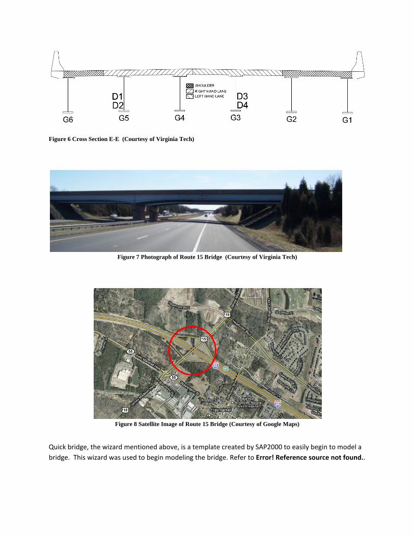
Figure 6 Cross Section E-E (Courtesy of Virginia Tech)
Figure 7 Photograph of Route 15 Bridge (Courtesy of Virginia Tech)
Figure 8 Satellite Image of Route 15 Bridge (Courtesy of Google Maps)
Quick bridge, the wizard mentioned above, is a template created by SAP2000 to easily begin to model a bridge. This wizard was used to begin modeling the bridge. Refer to Error! Reference source not found..
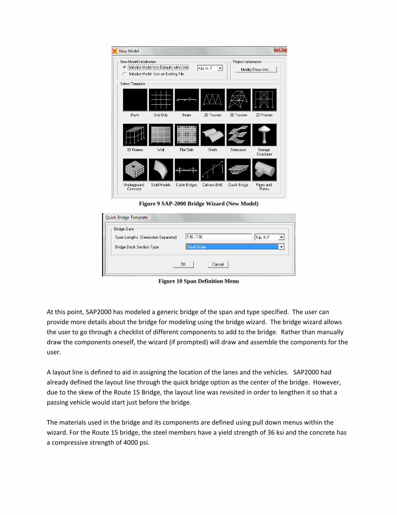
Figure 9 SAP-2000 Bridge Wizard (New Model)
Figure 10 Span Definition Menu
At this point, SAP2000 has modeled a generic bridge of the span and type specified. The user can provide more details about the bridge for modeling using the bridge wizard. The bridge wizard allows the user to go through a checklist of different components to add to the bridge. Rather than manually draw the components oneself, the wizard (if prompted) will draw and assemble the components for the user. A layout line is defined to aid in assigning the location of the lanes and the vehicles. SAP2000 had already defined the layout line through the quick bridge option as the center of the bridge. However, due to the skew of the Route 15 Bridge, the layout line was revisited in order to lengthen it so that a passing vehicle would start just before the bridge. The materials used in the bridge and its components are defined using pull down menus within the wizard. For the Route 15 bridge, the steel members have a yield strength of 36 ksi and the concrete has a compressive strength of 4000 psi.
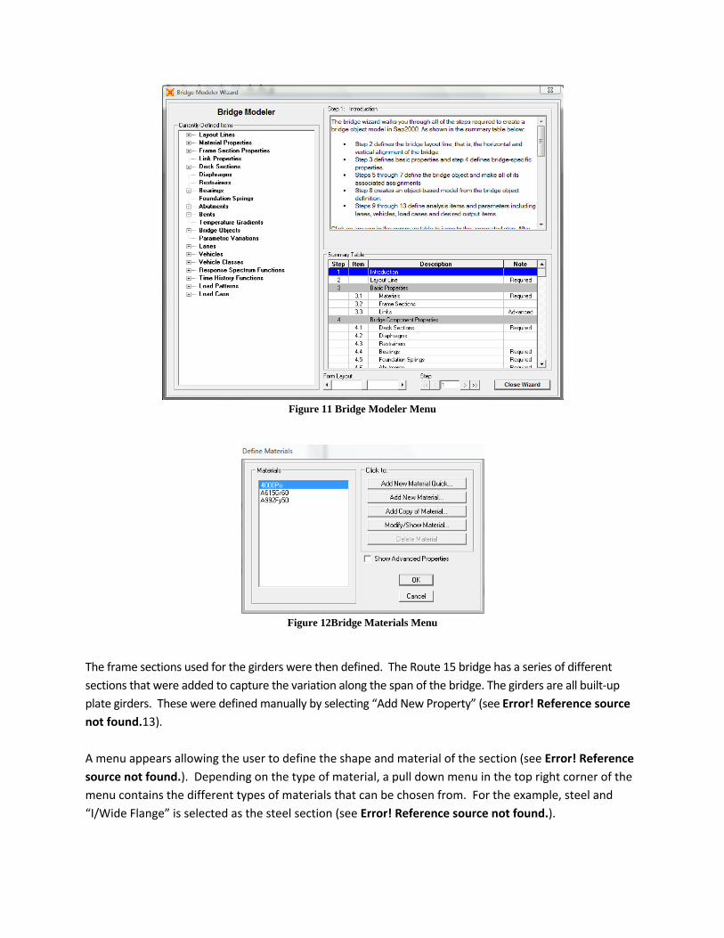
Figure 11 Bridge Modeler Menu
Figure 12Bridge Materials Menu
The frame sections used for the girders were then defined. The Route 15 bridge has a series of different sections that were added to capture the variation along the span of the bridge. The girders are all built-up plate girders. These were defined manually by selecting “Add New Property” (see Error! Reference source not found.13). A menu appears allowing the user to define the shape and material of the section (see Error! Reference source not found.). Depending on the type of material, a pull down menu in the top right corner of the menu contains the different types of materials that can be chosen from. For the example, steel and “I/Wide Flange” is selected as the steel section (see Error! Reference source not found.).

Figure 13 Frame Properties Menu
Figure 14 Section Definition menu
Figure 15 I/Wide Flange Definition Menu

For the Route 15 Bridge, one of the plate girders is composed of 16”x1” plates for the flanges and a 52”x3/8” plate for the web. The section was named to make it easily distinguishable from the other sections defined. The dimensions of the frame section are specified in the menu. Additionally, since there are diaphragms present in the bridge, additional frame sections were added. While the frame sections of the diaphragms are added at this time, the diaphragms were not added to the model until a later step. The diaphragms are made up of angle section and SAP-2000 contains a library of all standard sections for AISC steel shapes and their respective data and dimensions. The desired steel material (A36) and the angle L3½x3½x⅜ was selected. The other frame sections for the diaphragm components were chosen similarly. The bridge has a non-uniform cross section. As the span gets near the midpoint of the bridge, the web height increases parabolicly. All the necessary I-sections were created, including a representative section at the beginning of the parabolic curve and at the end. This bridge has three varying sections in each span for a total of six varying sections. Non-uniform, or non-prismatic, sections are available from the menus. Once the section has been named, choosing the starting and ending section as well as the overall shape of the curve (linear, parabolic, etc.) based on the previously defined sections. At a later time, the user will be able to assign the generated sections to different spans of the bridge.
Figure 16 Non-Prismatic Menu
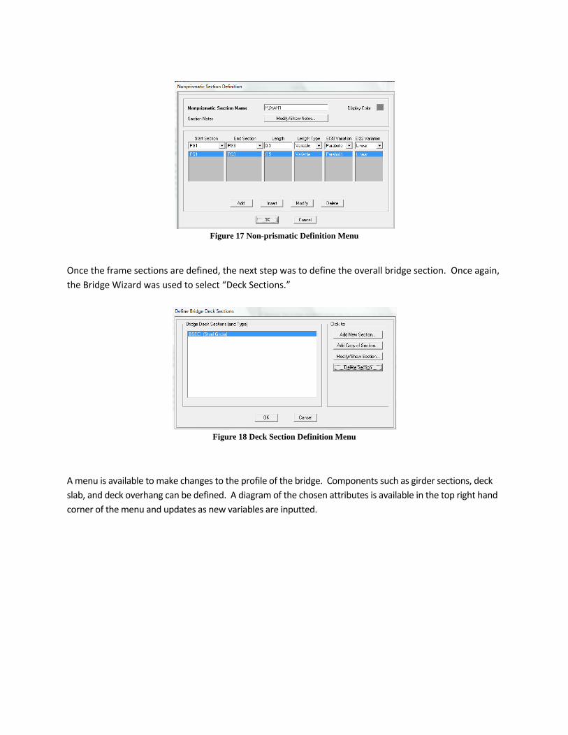
Figure 17 Non-prismatic Definition Menu
Once the frame sections are defined, the next step was to define the overall bridge section. Once again, the Bridge Wizard was used to select “Deck Sections.”
Figure 18 Deck Section Definition Menu
A menu is available to make changes to the profile of the bridge. Components such as girder sections, deck slab, and deck overhang can be defined. A diagram of the chosen attributes is available in the top right hand corner of the menu and updates as new variables are inputted.
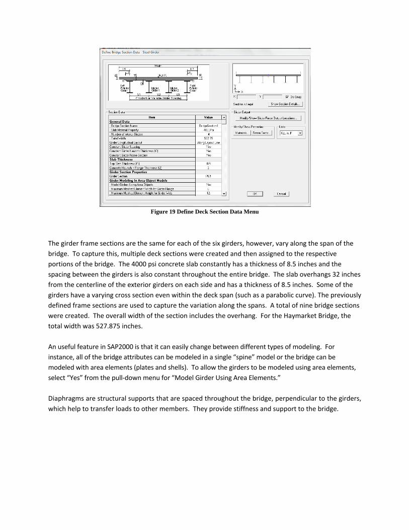
Figure 19 Define Deck Section Data Menu
The girder frame sections are the same for each of the six girders, however, vary along the span of the bridge. To capture this, multiple deck sections were created and then assigned to the respective portions of the bridge. The 4000 psi concrete slab constantly has a thickness of 8.5 inches and the spacing between the girders is also constant throughout the entire bridge. The slab overhangs 32 inches from the centerline of the exterior girders on each side and has a thickness of 8.5 inches. Some of the girders have a varying cross section even within the deck span (such as a parabolic curve). The previously defined frame sections are used to capture the variation along the spans. A total of nine bridge sections were created. The overall width of the section includes the overhang. For the Haymarket Bridge, the total width was 527.875 inches. An useful feature in SAP2000 is that it can easily change between different types of modeling. For instance, all of the bridge attributes can be modeled in a single “spine” model or the bridge can be modeled with area elements (plates and shells). To allow the girders to be modeled using area elements, select “Yes” from the pull-down menu for “Model Girder Using Area Elements.” Diaphragms are structural supports that are spaced throughout the bridge, perpendicular to the girders, which help to transfer loads to other members. They provide stiffness and support to the bridge.

Figure 20 Diaphragm Definition Menu
There are three options for bridge diaphragms, a solid diaphragm, a chord and brace diaphragm, or a single beam diaphragm. The solid diaphragm can only be used for a concrete bridge while the other two options can be used for a steel bridge. When defining a chord and brace diaphragm, the user has the option to decide among three different options: a V brace, an inverted V brace or an X brace. For the Route 15 bridge, the diaphragms are all chord and brace diaphragms with X braces. There were three different chord and brace diaphragms defined for this bridge. The diaphragms over the abutments and the pier have both a top chord and a bottom chord white the intermediate diaphragms only have a bottom chord. The frame sections for the diaphragm previously can be added.
Figure 21 Diaphragm Properties Menu
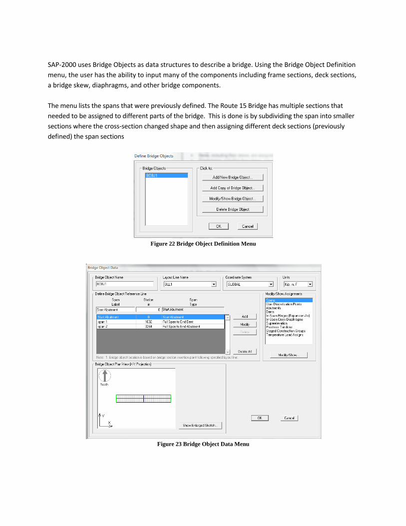
SAP-2000 uses Bridge Objects as data structures to describe a bridge. Using the Bridge Object Definition menu, the user has the ability to input many of the components including frame sections, deck sections, a bridge skew, diaphragms, and other bridge components. The menu lists the spans that were previously defined. The Route 15 Bridge has multiple sections that needed to be assigned to different parts of the bridge. This is done is by subdividing the span into smaller sections where the cross-section changed shape and then assigning different deck sections (previously defined) the span sections
Figure 22 Bridge Object Definition Menu
Figure 23 Bridge Object Data Menu
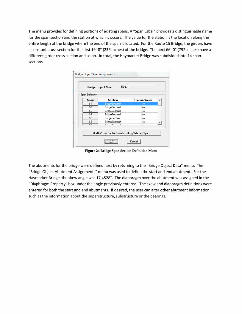
The menu provides for defining portions of existing spans. A “Span Label” provides a distinguishable name for the span section and the station at which it occurs. The value for the station is the location along the entire length of the bridge where the end of the span is located. For the Route 15 Bridge, the girders have a constant cross section for the first 19’-8” (236 inches) of the bridge. The next 66’-0” (792 inches) have a different girder cross section and so on. In total, the Haymarket Bridge was subdivided into 14 span sections.
Figure 24 Bridge Span Section Definition Menu
The abutments for the bridge were defined next by returning to the “Bridge Object Data” menu. The “Bridge Object Abutment Assignments” menu was used to define the start and end abutment. For the Haymarket Bridge, the skew angle was 17.4528°. The diaphragm over the abutment was assigned in the “Diaphragm Property” box under the angle previously entered. The skew and diaphragm definitions were entered for both the start and end abutments. If desired, the user can alter other abutment information such as the information about the superstructure, substructure or the bearings.
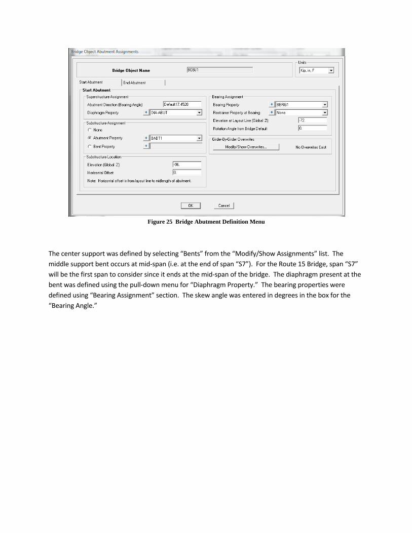
Figure 25 Bridge Abutment Definition Menu
The center support was defined by selecting “Bents” from the “Modify/Show Assignments” list. The middle support bent occurs at mid-span (i.e. at the end of span “S7”). For the Route 15 Bridge, span “S7” will be the first span to consider since it ends at the mid-span of the bridge. The diaphragm present at the bent was defined using the pull-down menu for “Diaphragm Property.” The bearing properties were defined using “Bearing Assignment” section. The skew angle was entered in degrees in the box for the “Bearing Angle.”
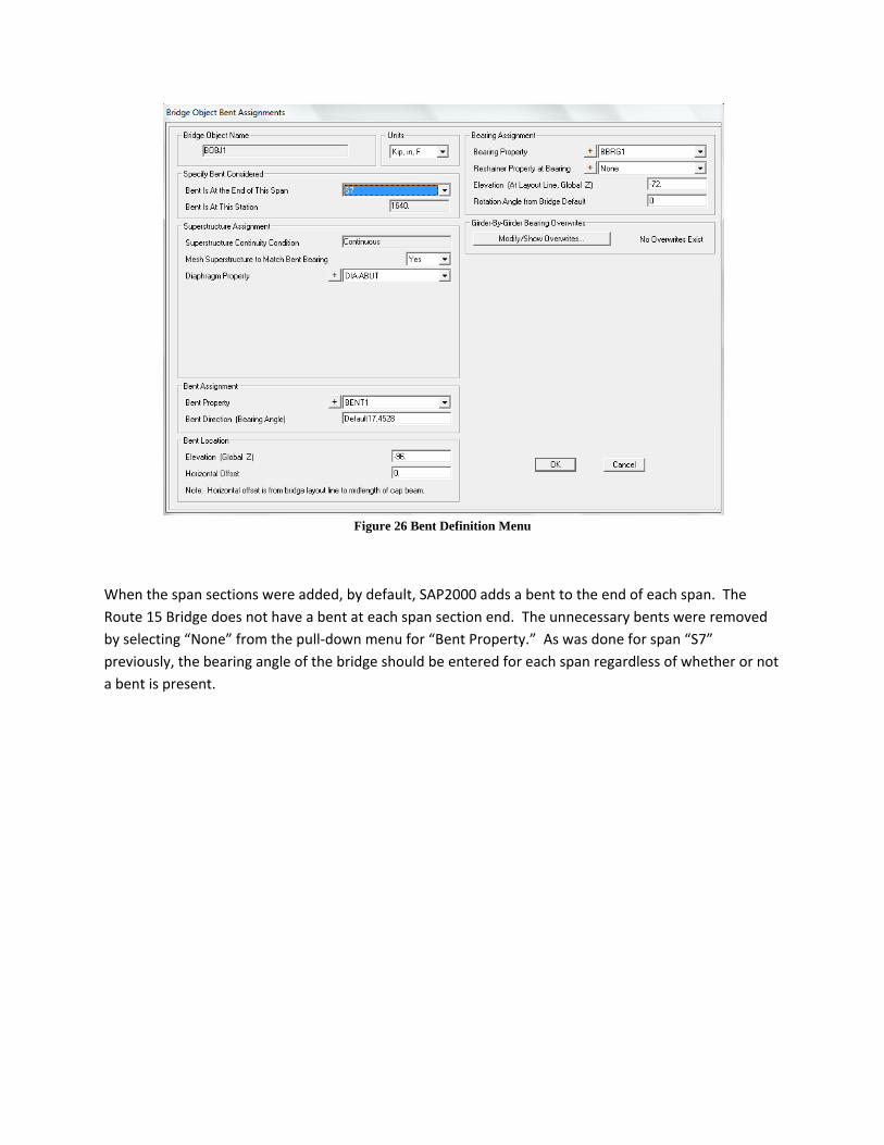
Figure 26 Bent Definition Menu
When the span sections were added, by default, SAP2000 adds a bent to the end of each span. The Route 15 Bridge does not have a bent at each span section end. The unnecessary bents were removed by selecting “None” from the pull-down menu for “Bent Property.” As was done for span “S7” previously, the bearing angle of the bridge should be entered for each span regardless of whether or not a bent is present.

Figure 27 Bent Data Assignment Menu
The diaphragms that were previously defined were assigned to their respective locations along the span of the bridge. The user must determine the distance into the span in which the diaphragm occurs. For example, one of the first diaphragms occurs at 280 inches from the start of the girder. Since span, “S1,” only has a length of 236 inches, the diaphragm will occur at 44 inches into span, “S2.” Therefore, to add the first diaphragm, span “S2” was selected along with the corresponding diaphragm. Then the distance of 44 inches was entered with the appropriate bearing angle. The other diaphragms were all added similarly.
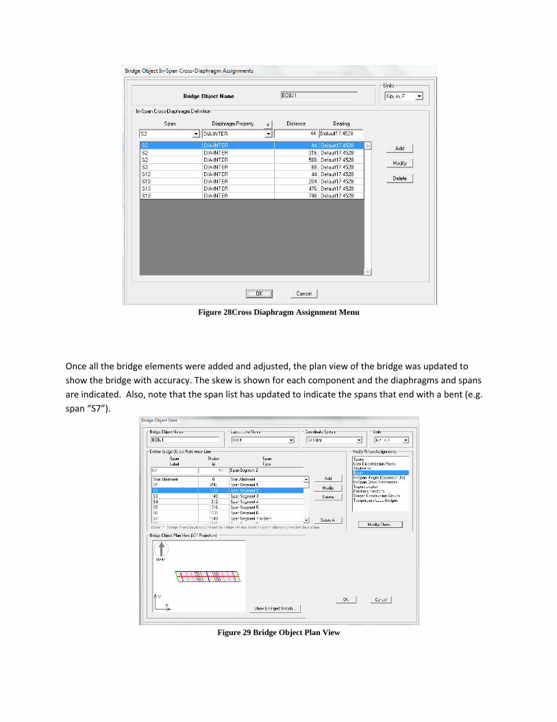
Figure 28Cross Diaphragm Assignment Menu
Once all the bridge elements were added and adjusted, the plan view of the bridge was updated to show the bridge with accuracy. The skew is shown for each component and the diaphragms and spans are indicated. Also, note that the span list has updated to indicate the spans that end with a bent (e.g. span “S7”).
Figure 29 Bridge Object Plan View

Once all the data has been input, the model be viewed using different types of elements. The difference between each level of modeling is the amount of detail that is depicted as well as the analysis time. There are three different types of models provided by SAP-2000. A spine model, an area and spine model, and a complete area model, each with increasing levels of detail and computational effort. A Solid Object Model is also available but was not considered for this problem due to the complexity. The different model options are accessed via the “Update Bridge Structural Model” menu. From the Bridge Wizard menu, select “Update Linked Model.” Once the menu has appeared, the right-hand column gives the modeling options.
Figure 30 Bridge Model Update Menu
The spine model using frame objects takes all of the bridge attributes and models them as one line. This type of model can be advantageous because the analysis will take much less time to run and it is fast to obtain the overall bridge response (including the deflected shape or moment diagram. However, a spine model will not physically show the details of the bridge, so incorrect modeling may easily be overlooked. For the Route 15 Bridge model, this level of modeling was inadequate because the influence surface is desired for many different points along the entire span of the bridge and not merely along the center. Also, since displacements can only be obtained at nodes, such a model would limit the amount of data attained since there are much fewer nodes present.

Figure 31 Spline Model
Two different types of area models can be created. One of the models depicts area elements for the deck and slab but the girders are modeled as spine elements, or girder lines as shown in Error! Reference source not found.. This model can be the best option if the girders have a uniform cross section throughout the entire length of the bridge since the varying cross section will not need to be shown. Due to the types of data that were desired for the Route 15 Bridge, this option was selected for the majority of the analysis work. It was necessary to have at least beam elements and multiple nodes rather than one encompassing spine model. The precision of the data was still very similar to the precision when using the next complex model and the analysis took much less time to run than an entire area model, one hour versus thirty hours.
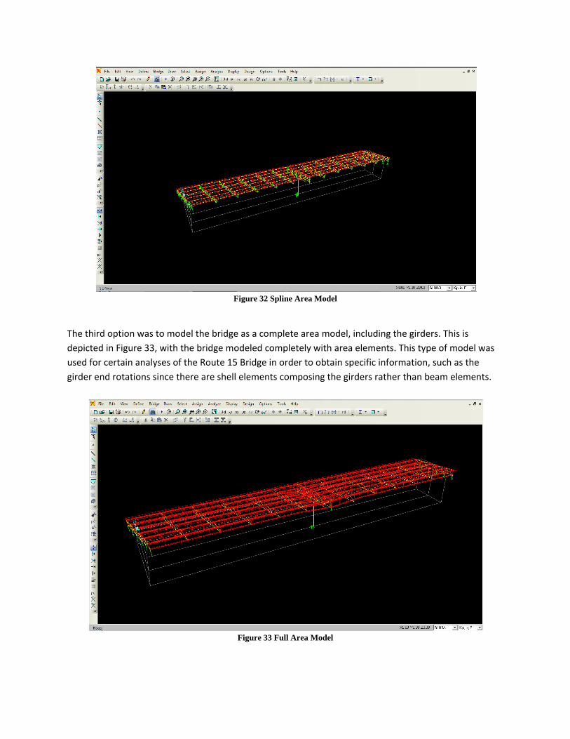
Figure 32 Spline Area Model
The third option was to model the bridge as a complete area model, including the girders. This is depicted in Figure 33, with the bridge modeled completely with area elements. This type of model was used for certain analyses of the Route 15 Bridge in order to obtain specific information, such as the girder end rotations since there are shell elements composing the girders rather than beam elements.
Figure 33 Full Area Model

SAP2000 defines lanes initially as part of the quick bridge. The principal purpose of the lanes is to specify the position of a moving load. Lanes can be straight or curved to model different vehicle movements . Generally, the user will create lanes to replicate those on the bridge in lane width and relative distance from the centerline of the bridge.
Figure 34 Lane Definition Menu
The “Bridge Lane Data” menu allows the user to input or modify data about the lane. Based on the location of the layout line defined from Quick Bridge, lanes can be created by offsetting from the layout line and the width can be entered. The plan view in the lower left corner will update to illustrate the lane in relation to the layout line. If the lanes defined by Quick Bridge are inadequate and new lanes must be added without using the layout line, the user can select “Add New Lane Defined from Frames.” The lane is the path defined by the order of the frames. This manner to create lanes is a good alternative; however, it is much faster to create the lanes based on the layout line. In the case of the Route 15 Bridge, there were a total of two straight lanes. However, because general influence surfaces were desired for the Route 15 bridge, additional lanes were defined order to obtain influence data for many point load locations.
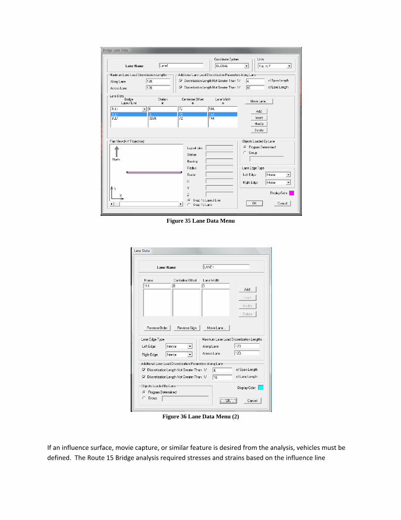
Figure 35 Lane Data Menu
Figure 36 Lane Data Menu (2)
If an influence surface, movie capture, or similar feature is desired from the analysis, vehicles must be defined. The Route 15 Bridge analysis required stresses and strains based on the influence line
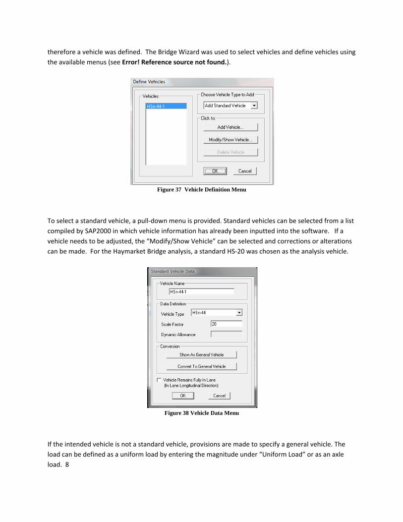
therefore a vehicle was defined. The Bridge Wizard was used to select vehicles and define vehicles using the available menus (see Error! Reference source not found.).
Figure 37 Vehicle Definition Menu
To select a standard vehicle, a pull-down menu is provided. Standard vehicles can be selected from a list compiled by SAP2000 in which vehicle information has already been inputted into the software. If a vehicle needs to be adjusted, the “Modify/Show Vehicle” can be selected and corrections or alterations can be made. For the Haymarket Bridge analysis, a standard HS-20 was chosen as the analysis vehicle.
Figure 38 Vehicle Data Menu
If the intended vehicle is not a standard vehicle, provisions are made to specify a general vehicle. The load can be defined as a uniform load by entering the magnitude under “Uniform Load” or as an axle load. 8

Figure 39 General Vehicle Data Menu
Vehicle classes are used to group vehicles together for the analysis. If only one vehicle is inputted to a vehicle class, then the response from just the one vehicle will be reported. If, however, more than one vehicle is in a vehicle class, the entire caravan of vehicles will be used in the analysis, but with the vehicles crossing the bridge one at a time
Figure 40 Vehicle Class Definition Menu

Figure 41 Vehicle Class Data Menu
In order to control the types of output created during an analysis involving a moving load, as well as the level of refinement of the output, the “Moving Load Case Results Saved” menu is used. This menu offers control over many output parameters including displacements, stresses, and reactions. Additionally, the “method of calculation” can also be adjusted either as exact or at some other refinement level. Some benefits of using this menu is that the analysis time can be drastically cut back depending on which parameters are adjusted.
Figure 42 Moving Load Results Selection Menu
Load patterns provide a way to load the bridge in different manners. The existing load patterns can be modified by editing the text boxes and selecting “Modify Load Pattern.” The user can also add new patterns by entering the new data and then selecting “Add New Load Pattern.” Loads patterns were each individually added to the Load Pattern list for the Haymarket Bridge.

Figure 43 Load Pattern Definition Menu
There are many additional load pattern types that can be defined by selecting “Other” from the “Type” pull-down menu. Some options are available including Pedestrian Live Load, Bridge Live Load, and Quake Load. If a linear multi-step static load case is desired for the analysis, it is necessary to add a “Bridge Live” load pattern to the list. Once the Bridge Live load is on the load pattern list, select “Modify Bridge Live Load” to view the “Multi Step Live Load Pattern Generation” menu.
Figure 44 Multi-step Live Load Pattern Generation Menu
From the multi step menu, the user can input specific parameters about the load pattern such as the type of vehicle that drives across a specific lane. The speed of the vehicle and the load duration can be identified as well. This information enables SAP2000 to generate the load steps and a movie capture of the vehicle if desired. Load cases include the various types of loadings that the bridge experiences due to different sources. Rather than lumping all the loads into one value, SAP2000 allows the user to input the magnitudes and directions of the different types of loads including the dead loads, live loads, etc. The software has the capability for the loads to be applied linearly or nonlinearly to the structure. Load cases are specifies using “Load Cases” from the Bridge Wizard. The “Define Load Cases” menu will appear and will display the load cases that are defined. By default, three load cases will have already been defined, including dead, modal, and moving loads.
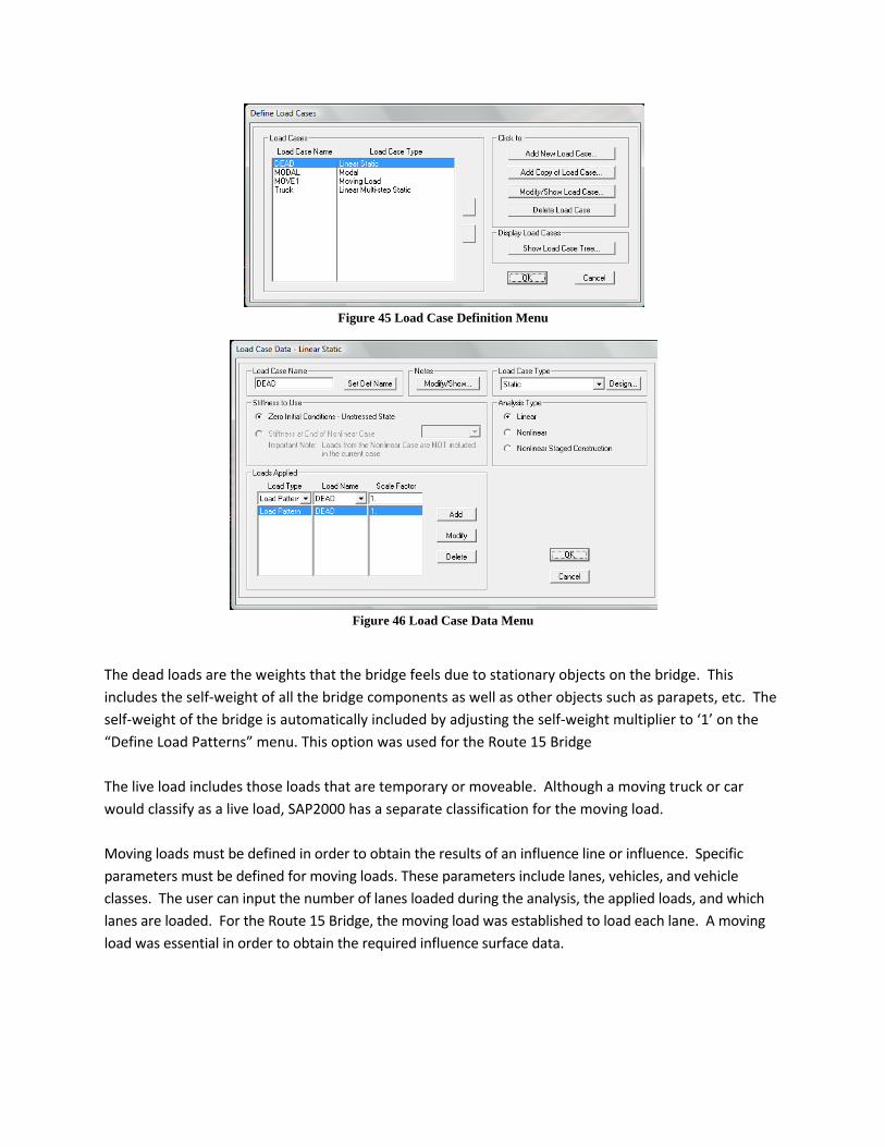
Figure 45 Load Case Definition Menu
Figure 46 Load Case Data Menu
The dead loads are the weights that the bridge feels due to stationary objects on the bridge. This includes the self-weight of all the bridge components as well as other objects such as parapets, etc. The self-weight of the bridge is automatically included by adjusting the self-weight multiplier to ‘1’ on the “Define Load Patterns” menu. This option was used for the Route 15 Bridge The live load includes those loads that are temporary or moveable. Although a moving truck or car would classify as a live load, SAP2000 has a separate classification for the moving load.
Moving loads must be defined in order to obtain the results of an influence line or influence. Specific parameters must be defined for moving loads. These parameters include lanes, vehicles, and vehicle classes. The user can input the number of lanes loaded during the analysis, the applied loads, and which lanes are loaded. For the Route 15 Bridge, the moving load was established to load each lane. A moving load was essential in order to obtain the required influence surface data.
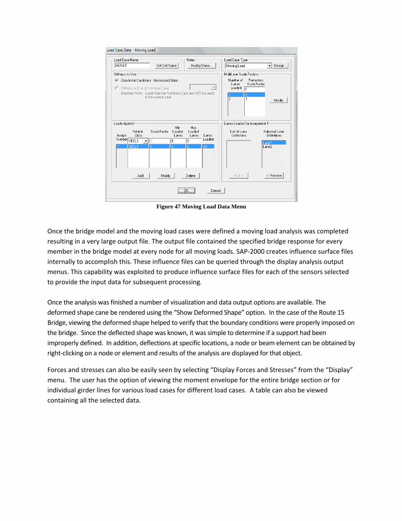
Figure 47 Moving Load Data Menu
Once the bridge model and the moving load cases were defined a moving load analysis was completed resulting in a very large output file. The output file contained the specified bridge response for every member in the bridge model at every node for all moving loads. SAP-2000 creates influence surface files internally to accomplish this. These influence files can be queried through the display analysis output menus. This capability was exploited to produce influence surface files for each of the sensors selected to provide the input data for subsequent processing. Once the analysis was finished a number of visualization and data output options are available. The deformed shape cane be rendered using the “Show Deformed Shape” option. In the case of the Route 15 Bridge, viewing the deformed shape helped to verify that the boundary conditions were properly imposed on the bridge. Since the deflected shape was known, it was simple to determine if a support had been improperly defined. In addition, deflections at specific locations, a node or beam element can be obtained by right-clicking on a node or element and results of the analysis are displayed for that object.
Forces and stresses can also be easily seen by selecting “Display Forces and Stresses” from the “Display” menu. The user has the option of viewing the moment envelope for the entire bridge section or for individual girder lines for various load cases for different load cases. A table can also be viewed containing all the selected data.

Figure 48 Deflected Shape View
Of particular importance to this project is the ability to visualize and output influence surfaces. The “Show Influence Line/Surface” menu allows the user to specify for what object the influence surface will be displayed. Depending on the lanes that were previously defined, the user can select the lanes in which the influence data will be reported for. For the Route 15 Bridge two travel lanes were specified. Depending on the manner in which the user wants to view the information, either a table of data can be obtained or the influence surface can be imposed on the undeformed rendering of the model. For the analysis of the Route 15 Bridge, the information was most useful in tabular form because the data was needed for interpolation and simulation purposes. Once the desired table of data appears, the data can be pasted into an Excel Spreadsheet for further evaluation. This capability was used to transfer the influence surface files from SAP-2000 to Excel for subsequent use.
To collect moment influence data for the Route 15 Bridge, frame data was used to specify the exact location of the sensors for moment data was required. When “Frame” is selected from the “Show Influence Line/Surface” menu, the menu changes to display different output variables (including shear and moment). When a frame element is selected, the user must input the location along the frame for which the influence surface data is desired. For the Route 15 Bridge, influence data was desired specific sensor locations. The sensor locations were 653 inches and 2611 inches along Girders 3 and 5 respectively.
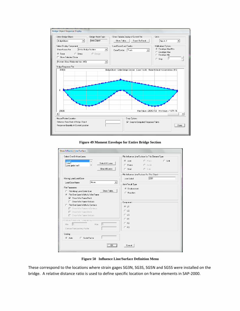
Figure 49 Moment Envelope for Entire Bridge Section
Figure 50 Influence Line/Surface Definition Menu
These correspond to the locations where strain gages SG3N, SG3S, SG5N and SG5S were installed on the bridge. A relative distance ratio is used to define specific location on frame elements in SAP-2000.
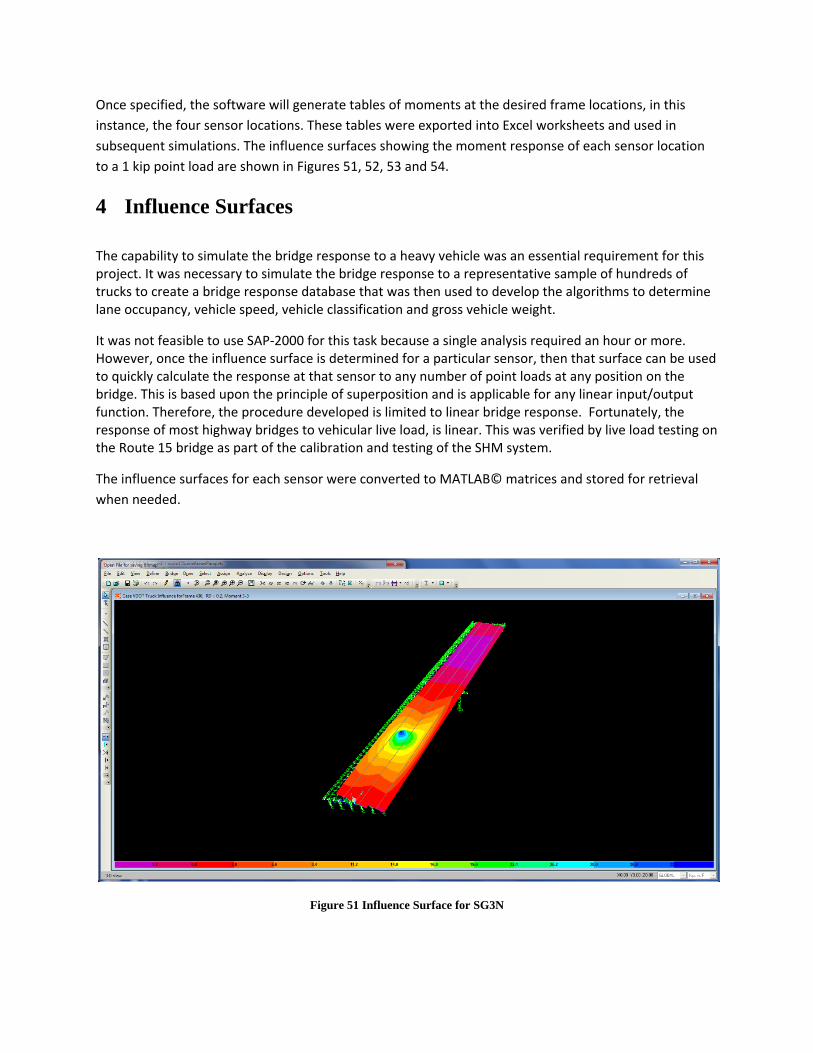
Once specified, the software will generate tables of moments at the desired frame locations, in this instance, the four sensor locations. These tables were exported into Excel worksheets and used in subsequent simulations. The influence surfaces showing the moment response of each sensor location to a 1 kip point load are shown in Figures 51, 52, 53 and 54.
4 Influence Surfaces
The capability to simulate the bridge response to a heavy vehicle was an essential requirement for this project. It was necessary to simulate the bridge response to a representative sample of hundreds of trucks to create a bridge response database that was then used to develop the algorithms to determine lane occupancy, vehicle speed, vehicle classification and gross vehicle weight.
It was not feasible to use SAP-2000 for this task because a single analysis required an hour or more. However, once the influence surface is determined for a particular sensor, then that surface can be used to quickly calculate the response at that sensor to any number of point loads at any position on the bridge. This is based upon the principle of superposition and is applicable for any linear input/output function. Therefore, the procedure developed is limited to linear bridge response. Fortunately, the response of most highway bridges to vehicular live load, is linear. This was verified by live load testing on the Route 15 bridge as part of the calibration and testing of the SHM system.
The influence surfaces for each sensor were converted to MATLAB© matrices and stored for retrieval when needed.
Figure 51 Influence Surface for SG3N
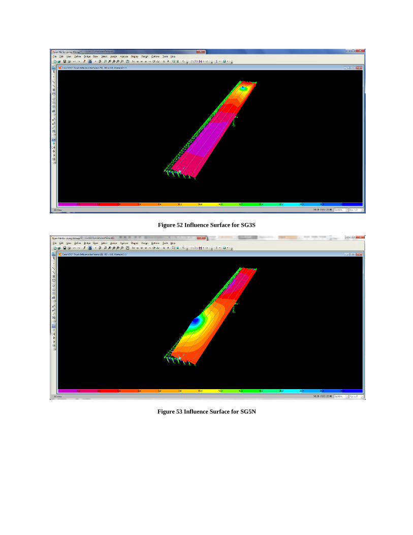
Figure 52 Influence Surface for SG3S
Figure 53 Influence Surface for SG5N
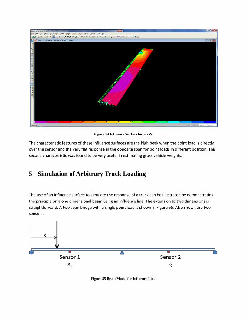
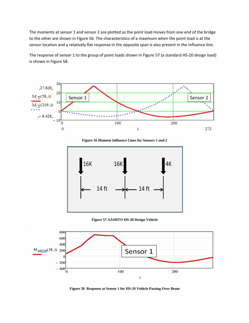
Figure 54 Influence Surface for SG5S
The characteristic features of these influence surfaces are the high peak when the point load is directly over the sensor and the very flat response in the opposite span for point loads in different position. This second characteristic was found to be very useful in estimating gross vehicle weights.
5 Simulation of Arbitrary Truck Loading
The use of an influence surface to simulate the response of a truck can be illustrated by demonstrating the principle on a one dimensional beam using an influence line. The extension to two dimensions is straightforward. A two span bridge with a single point load is shown in Figure 55. Also shown are two sensors.
Figure 55 Beam Model for Influence Line
The moments at sensor 1 and sensor 2 are plotted as the point load moves from one end of the bridge to the other are shown in Figure 56. The characteristics of a maximum when the point load is at the sensor location and a relatively flat response in the opposite span is also present in the influence line.
The response of sensor 1 to the group of point loads shown in Figure 57 (a standard HS-20 design load) is shown in Figure 58.
Figure 56 Moment Influence Lines for Sensors 1 and 2
Figure 57 AASHTO HS-20 Design Vehicle
Figure 58 Response at Sensor 1 for HS-20 Vehicle Passing Over Beam

A MATLAB© function (route15bridgesimulation7) was created to simulate the response at any of the four sensors to the passage of an arbitrary vehicle traveling in either of the two traffic lanes at any speed. The code for all function referenced are included in an appendix to this report. The function is passed the lane #, the sensor #, the speed and a matrix containing data describing the truck and returns three vectors, time in seconds for the vehicle position, an x coordinate of the position of the front axle of the truck and a vector of strain values at the specified sensor associated with each time and x coordinate value. A subordinate function, on bridge, is used to determine if a particular tire is on the bridge or not. This is necessary because tires move onto and off of the bridge during a truck passage.
This function was used to simulate the bridge response to random truck loads.
6 Generation of Random SU3 and 3-S2 Bridge Response Database
The literature review documented that two classes of heavy vehicles dominate the truck fleet in the United States. These are a three axle single unit truck, designated SU3, and a five axle semi-tractor trailer combination, designated 3-S2. These two vehicle classes were the focus of this study. The procedure developed classifies heavy trucks as either of these two classes. A bridge response database was created by generating hundreds of virtual SU3 and 3-S2 trucks with random variation of payload (the difference between the gross vehicle weight of a vehicle and its tare (empty) weight), axle spacing, and gauge (the distance between the wheels). These virtual trucks were passed to the route15bridgesimulation7 function. The bridge response database was created using two additional MATLAB© function, GenerateRandomSU3Trucks and GenerateRandom3S2Trucks. These functions accept a single argument, the number of virtual trucks to simulate, and return four vectors. A vector of random gross vehicle weights, a vector of time, x coordinates and strain values at a specific sensor. The characteristics of the SU3 vehicle used were based upon FHWA’s Truck Size and Weight reports. The SU3 vehicle used in this study is shown in Figure 59. The maximum legal load for this vehicle has a nominal value of 48,000 pounds. However it is not uncommon for vehicles of this class to have higher gross vehicle weights (GVW) with or without permits. The distribution of the GVW to the axles and tires is also shown in Figure 59. This is for the fully loaded case. For other loading cases, where the payload is variable, the following equations were used to distribute the GVW weight to the axles.
1
2
3
10 6 *( 22.6 ) / 25.4
6.2 9.8 *( 22.6 ) / 25.4
6.2 9.8 *( 22.6 ) / 25.4
axle
axle
axle
W K K GVW K K
W K K GVW K K
W K K GVW K K
= + −
= + −
= + −

Figure 59 Definition of SU3 Truck
The response of sensor SG3N to a nominal fully loaded SU3 truck traveling in lane 1 at different speeds is shown in Figure 60. The response traces are all very similar with different time bases as expected. In order to capture the effect of variations in payload, axle spacing and gauge a MatLab© routine was used to generate random vehicles. Note that the maximum GVW is limited to 48 Kip. The response of SG3N to 10 random trucks in Lane 1 traveling at 40 mph is shown in Figure 61. The same approach was used to generate random events for the 3-S2 vehicles but with additional axles and higher GVW.
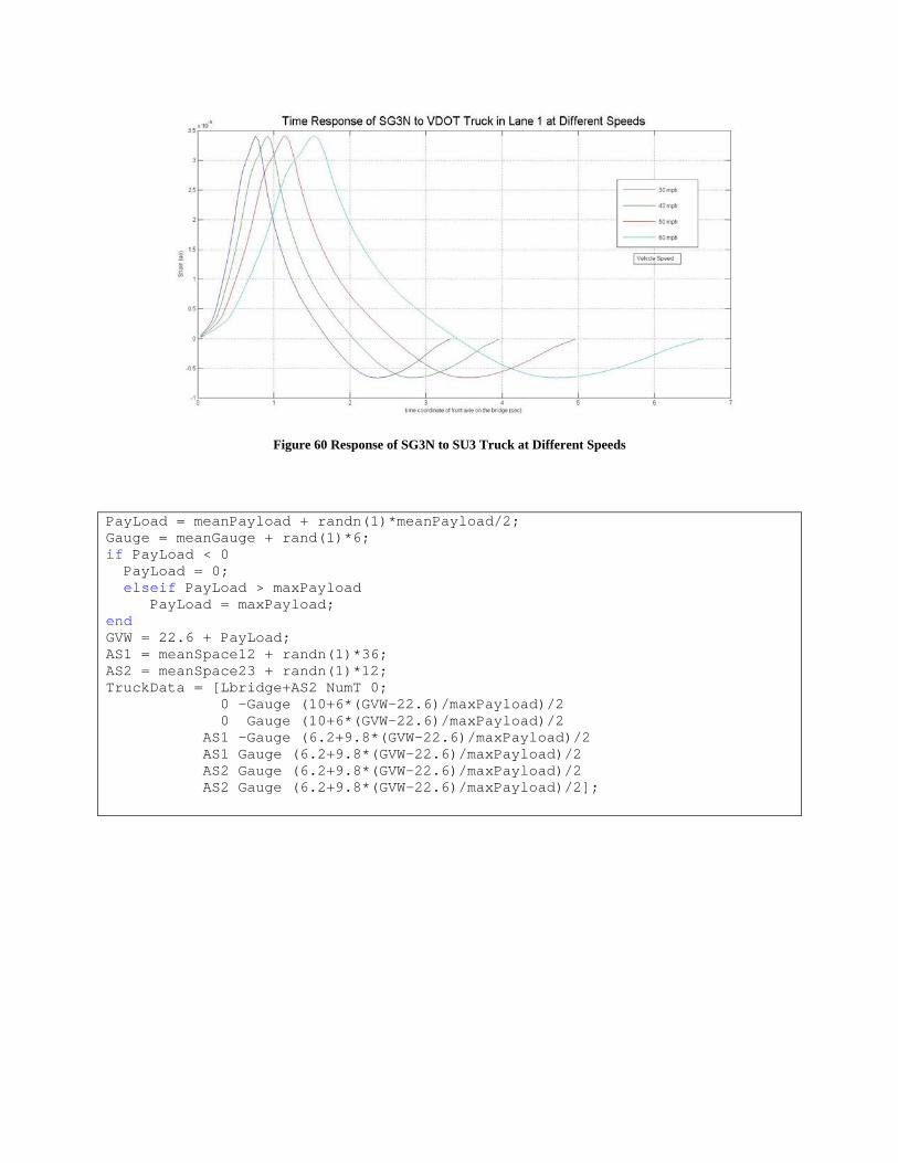
Figure 60 Response of SG3N to SU3 Truck at Different Speeds
PayLoad = meanPayload + randn(1)*meanPayload/2; Gauge = meanGauge + rand(1)*6; if PayLoad < 0 PayLoad = 0; elseif PayLoad > maxPayload PayLoad = maxPayload; end GVW = 22.6 + PayLoad; AS1 = meanSpace12 + randn(1)*36; AS2 = meanSpace23 + randn(1)*12; TruckData = [Lbridge+AS2 NumT 0; 0 -Gauge (10+6*(GVW-22.6)/maxPayload)/2 0 Gauge (10+6*(GVW-22.6)/maxPayload)/2 AS1 -Gauge (6.2+9.8*(GVW-22.6)/maxPayload)/2 AS1 Gauge (6.2+9.8*(GVW-22.6)/maxPayload)/2 AS2 Gauge (6.2+9.8*(GVW-22.6)/maxPayload)/2 AS2 Gauge (6.2+9.8*(GVW-22.6)/maxPayload)/2];
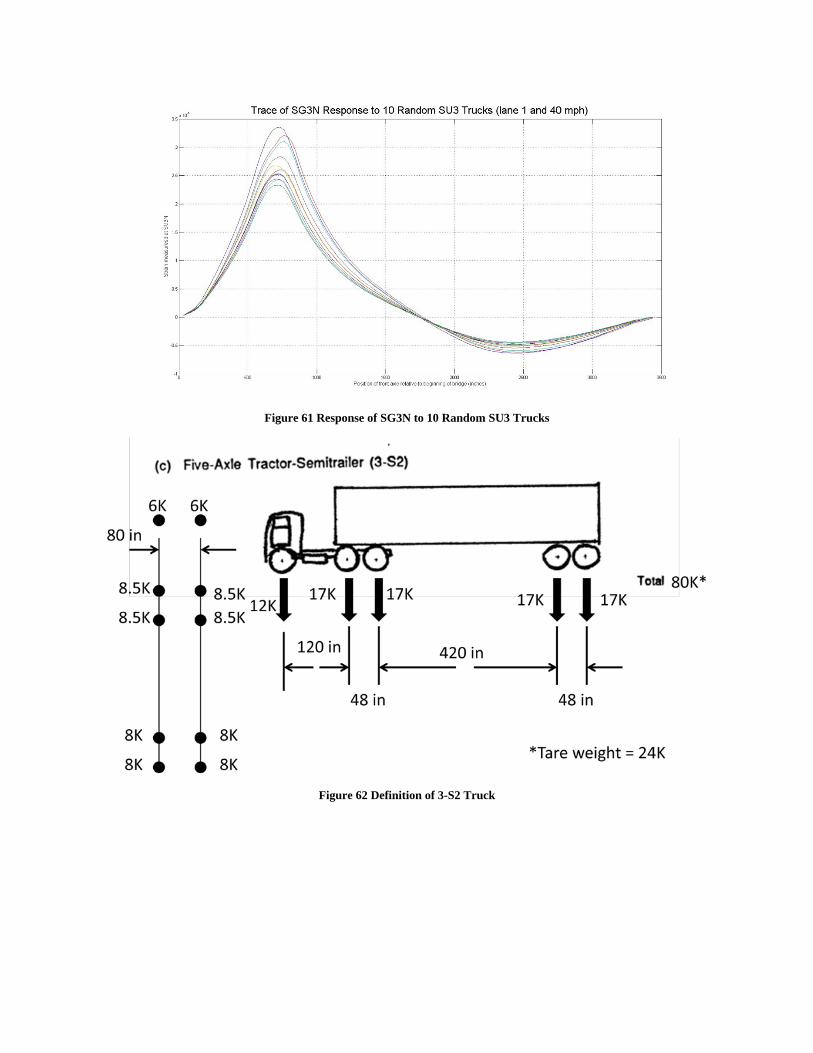
Figure 61 Response of SG3N to 10 Random SU3 Trucks
Figure 62 Definition of 3-S2 Truck
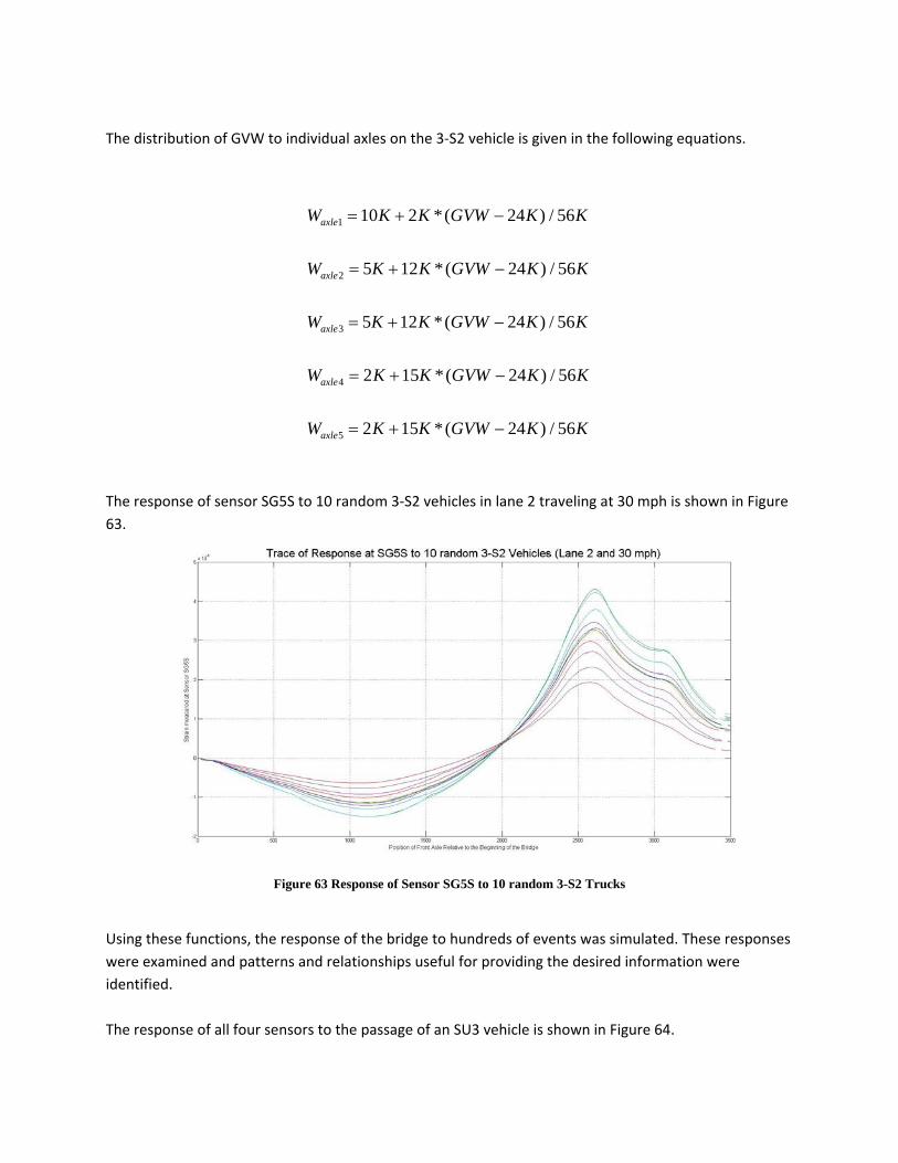
The distribution of GVW to individual axles on the 3-S2 vehicle is given in the following equations. The response of sensor SG5S to 10 random 3-S2 vehicles in lane 2 traveling at 30 mph is shown in Figure 63.
Figure 63 Response of Sensor SG5S to 10 random 3-S2 Trucks
Using these functions, the response of the bridge to hundreds of events was simulated. These responses were examined and patterns and relationships useful for providing the desired information were identified. The response of all four sensors to the passage of an SU3 vehicle is shown in Figure 64.
1
2
3
4
5
10 2 *( 24 ) / 56
5 12 *( 24 ) / 56
5 12 *( 24 ) / 56
2 15 *( 24 ) / 56
2 15 *( 24 ) / 56
axle
axle
axle
axle
axle
W K K GVW K K
W K K GVW K K
W K K GVW K K
W K K GVW K K
W K K GVW K K
= + −
= + −
= + −
= + −
= + −
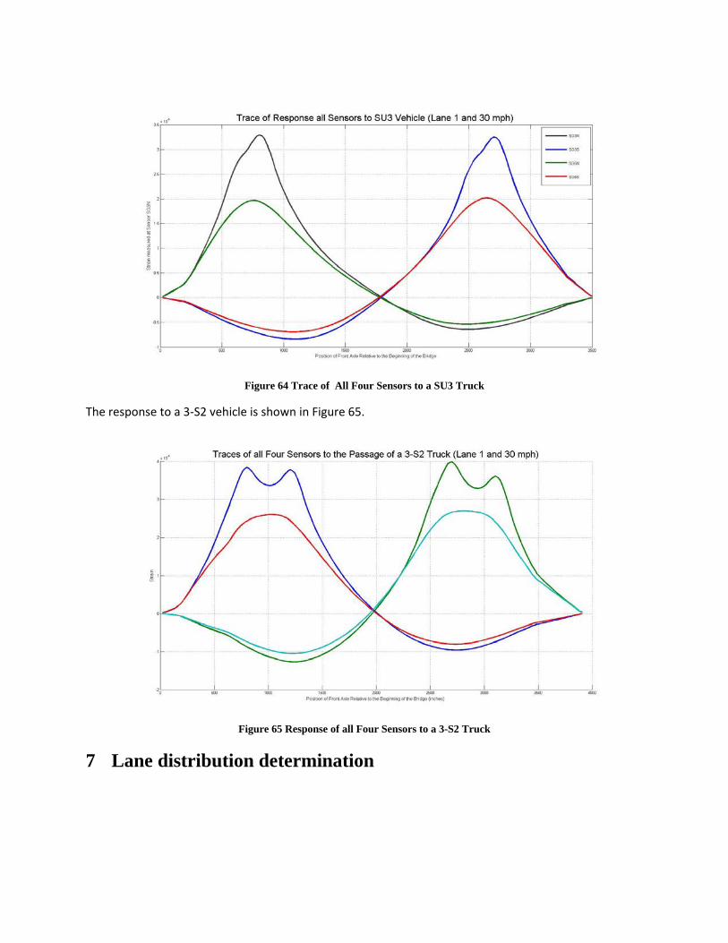
Figure 64 Trace of All Four Sensors to a SU3 Truck
The response to a 3-S2 vehicle is shown in Figure 65.
Figure 65 Response of all Four Sensors to a 3-S2 Truck
7 Lane distribution determination

It was noted that for all truck event simulations the ratio of the peak positive strain for SG3N and the peak positive strain for SG5N were greater than 1 when the vehicle was in lane 1 and was less than 1 when the vehicle was in lane 2.
Figure 66 SG3N/SG5N Ratios for Lane 1 and 2
This relationship held for all truck events. The ration SG3N/SG5N was calculated for the maximum positive strain value and was the lane occupation classifier for all truck events.
8 Speed determination
The relationship that was found useful for calculating vehicle speed was the time lag between the peak positive strain events for the sensors on the same girder line. This time lag is present in Figures 68 and 69. The peak positive strain on sensor SG3N occurs at 2.28 seconds. The corresponding peak strain occurs on sensor SG3S at 7.45 seconds. The distance along Girder 3 between sensor SG3N and Sensor SG3S is 1953 inches. With this known distance and time difference a speed can be calculated.

mphonds
inchesdtdx 8.20
sec)28.245.7(1953
=−
=
Figure 67 Lane Occupancy Determination
.

Figure 68 Traces for 3-S2 Vehicle at 20 MPH
Figure 69 Traces for SU3 Vehicle at 60 MPH
The second example is for a SU3 vehicle traveling at 60 mph in lane 1. Similar speed calculations utilizing the time lag between the peak values produce the following results.
mphonds
inchesdtdx 8.61
sec)76.056.2(1953
=−
=
The accuracy is dependent upon the sampling rate and measurement precision, but an estimate of vehicle speed within 5 percent appears very achievable. This procedure was used to determine vehicle speed for all truck events.
9 Vehicle classification
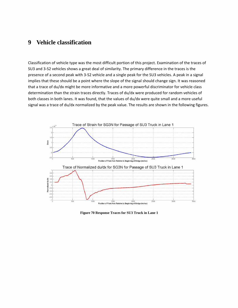
Classification of vehicle type was the most difficult portion of this project. Examination of the traces of SU3 and 3-S2 vehicles shows a great deal of similarity. The primary difference in the traces is the presence of a second peak with 3-S2 vehicle and a single peak for the SU3 vehicles. A peak in a signal implies that these should be a point where the slope of the signal should change sign. It was reasoned that a trace of du/dx might be more informative and a more powerful discriminator for vehicle class determination than the strain traces directly. Traces of du/dx were produced for random vehicles of both classes in both lanes. It was found, that the values of du/dx were quite small and a more useful signal was a trace of du/dx normalized by the peak value. The results are shown in the following figures.
Figure 70 Response Traces for SU3 Truck in Lane 1

Figure 71 Response Traces for SU3 in Lane 2
Figure 72 Response Traces for 3-S2 Truck in Lane 1

Figure 73 Response Traces for 3-S2 in Lane 2
As expected, the normalize du/dx trace showed a significant difference between SU3 and 3-S2 vehicles. This difference is the “bump” in the trace which is present for 3-S2 vehicles and absent for SU3 vehicles. It is probably associated with the rear tandem axle group. This “bump” has different magnitudes and a quantitative threshold was not found to be useful.
Figure 74 Empirically Determined Classification Feature Vector
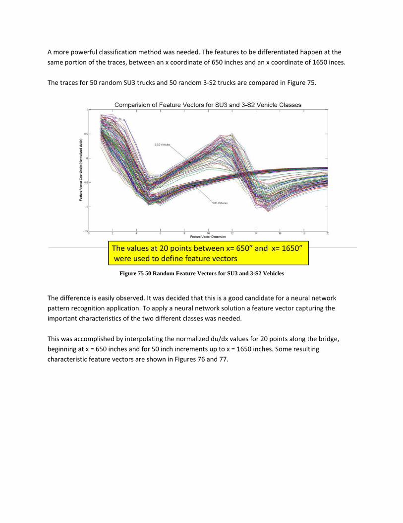
A more powerful classification method was needed. The features to be differentiated happen at the same portion of the traces, between an x coordinate of 650 inches and an x coordinate of 1650 inces. The traces for 50 random SU3 trucks and 50 random 3-S2 trucks are compared in Figure 75.
Figure 75 50 Random Feature Vectors for SU3 and 3-S2 Vehicles
The difference is easily observed. It was decided that this is a good candidate for a neural network pattern recognition application. To apply a neural network solution a feature vector capturing the important characteristics of the two different classes was needed. This was accomplished by interpolating the normalized du/dx values for 20 points along the bridge, beginning at x = 650 inches and for 50 inch increments up to x = 1650 inches. Some resulting characteristic feature vectors are shown in Figures 76 and 77.
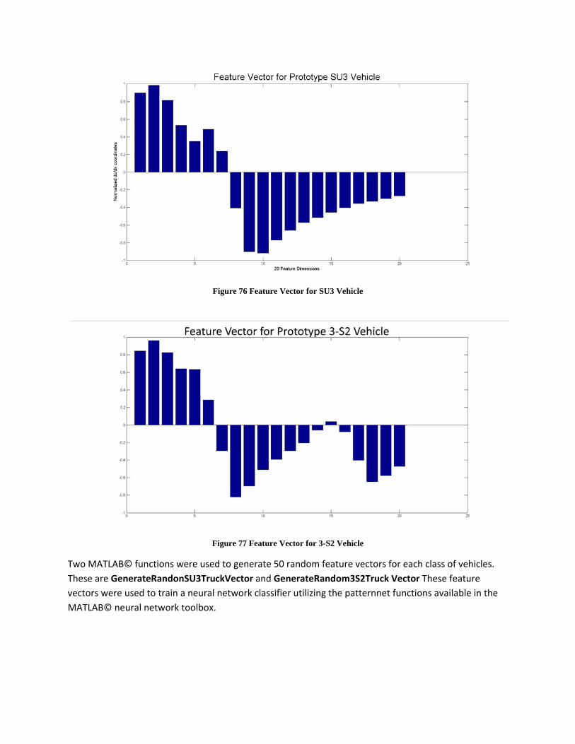
Figure 76 Feature Vector for SU3 Vehicle
Figure 77 Feature Vector for 3-S2 Vehicle
Two MATLAB© functions were used to generate 50 random feature vectors for each class of vehicles. These are GenerateRandonSU3TruckVector and GenerateRandom3S2Truck Vector These feature vectors were used to train a neural network classifier utilizing the patternnet functions available in the MATLAB© neural network toolbox.
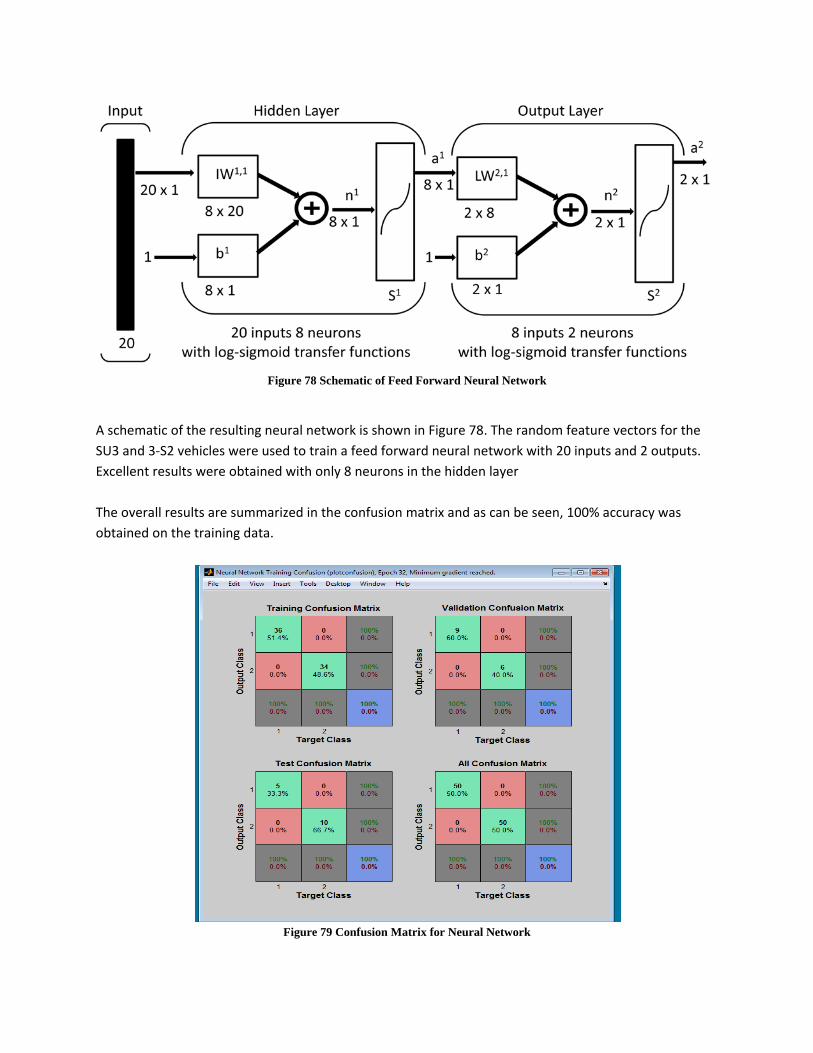
Figure 78 Schematic of Feed Forward Neural Network
A schematic of the resulting neural network is shown in Figure 78. The random feature vectors for the SU3 and 3-S2 vehicles were used to train a feed forward neural network with 20 inputs and 2 outputs. Excellent results were obtained with only 8 neurons in the hidden layer The overall results are summarized in the confusion matrix and as can be seen, 100% accuracy was obtained on the training data.
Figure 79 Confusion Matrix for Neural Network

At first it was thought that two networks would be needed, one for vehicle in lane 1 and another for vehicles in lane 2. It turned out that a single neural network classifier was able to accurately classify vehicle classes for both lanes. The trained neural network was used to classify SU3 and 3-S2 vehicles.
10 Gross vehicle weight estimation
The final task for extracting useful information from the SHM data was to estimate gross vehicle weight. At first, an investigation of the use of the maximum positive strain response was performed. The maximum response of all four sensors to 100 random 3-S2 trucks is shown in Figure 80.
Figure 80 Relation Between Peak Positive Strain and GVW
The linear relationship between maximum strain and GVW is obvious. However the response is also affected by variations in axle spacing and gauge, especially for the upstream sensors. The upstream sensors are located at the peak of the influence surface. It was observed that the influence surfaces for all gages had a characteristically flat region in the span opposite that for which the sensor is installed. This was found to be useful in estimating gross vehicle weight. The minimum negative strain for all sensors was determined for 100 random SU3 trucks in lanes 1 and 2. The results are shown in Figures 81 and 82.

Figure 81 Relationship Between Minimum Strain and GVW, SU3 in Lane 1
The linear relationship between minimum strain for all sensors in striking. The best GVW predictor for SU3 vehicles in lane 1 is the regression equation for SG3S. The best GVW predictor for SU3 vehicles in lane 2 is the regression equation for SG5S.
Figure 82 Relationship Between Minimum Strain and GVW, SU3 in Lane 2
A similar procedure was used to develop GVW estimators for 3-S2 vehicles.
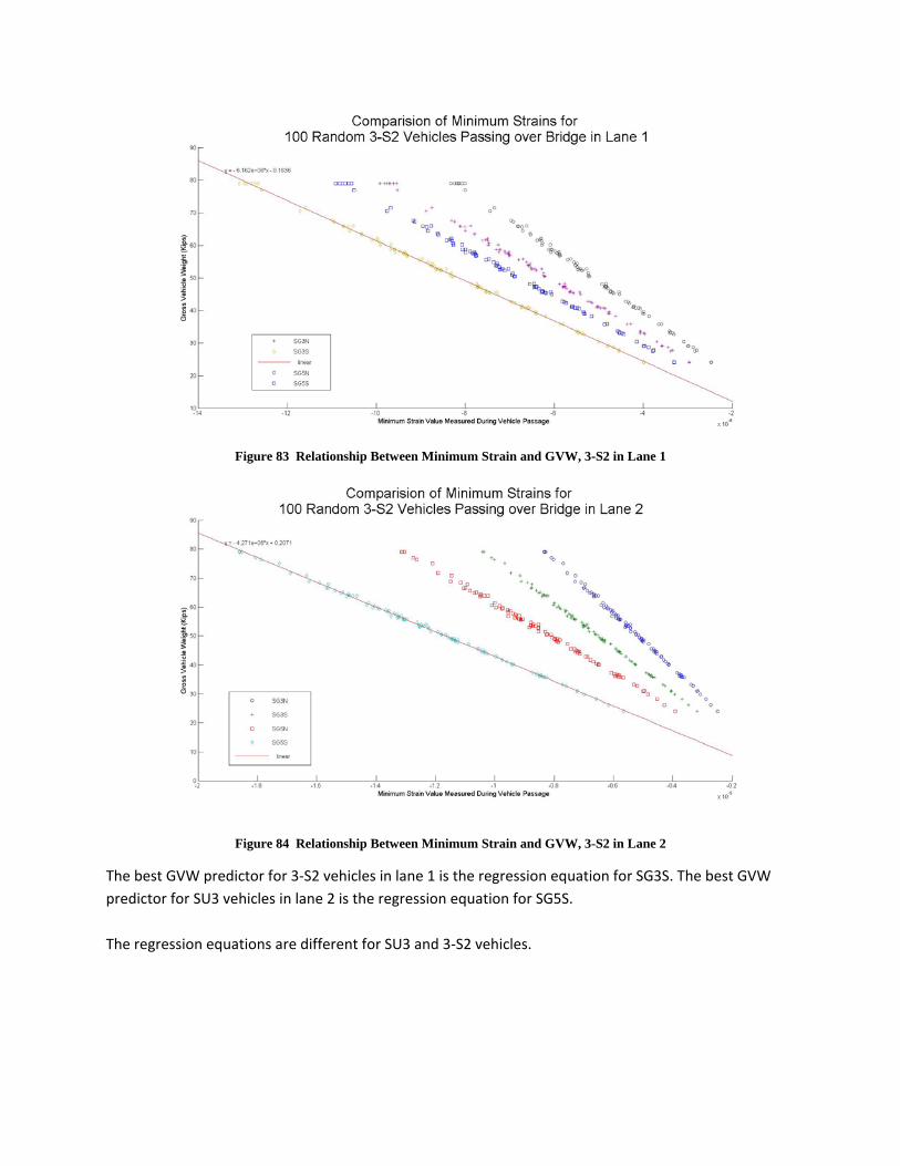
Figure 83 Relationship Between Minimum Strain and GVW, 3-S2 in Lane 1
Figure 84 Relationship Between Minimum Strain and GVW, 3-S2 in Lane 2
The best GVW predictor for 3-S2 vehicles in lane 1 is the regression equation for SG3S. The best GVW predictor for SU3 vehicles in lane 2 is the regression equation for SG5S. The regression equations are different for SU3 and 3-S2 vehicles.
11 Validation using actual truck data
To evaluate and demonstrate the utility of the procedure presented it was used to extract lane occupancy, speed, vehicle class and GVW from actual data obtained from the SHM system.
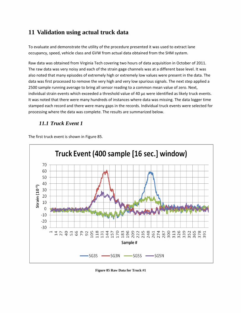
Raw data was obtained from Virginia Tech covering two hours of data acquisition in October of 2011. The raw data was very noisy and each of the strain gage channels was at a different base level. It was also noted that many episodes of extremely high or extremely low values were present in the data. The data was first processed to remove the very high and very low spurious signals. The next step applied a 2500 sample running average to bring all sensor reading to a common mean value of zero. Next, individual strain events which exceeded a threshold value of 40 με were identified as likely truck events. It was noted that there were many hundreds of instances where data was missing. The data logger time stamped each record and there were many gaps in the records. Individual truck events were selected for processing where the data was complete. The results are summarized below.
11.1 Truck Event 1
The first truck event is shown in Figure 85.
Figure 85 Raw Data for Truck #1
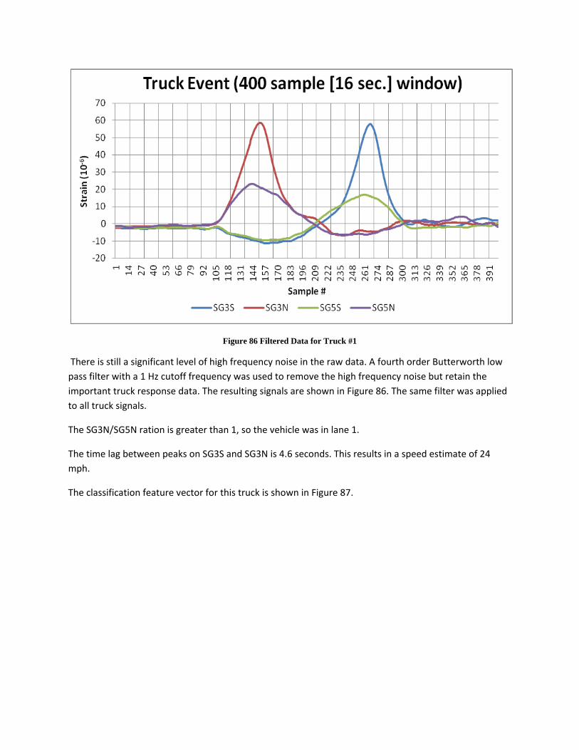
Figure 86 Filtered Data for Truck #1
There is still a significant level of high frequency noise in the raw data. A fourth order Butterworth low pass filter with a 1 Hz cutoff frequency was used to remove the high frequency noise but retain the important truck response data. The resulting signals are shown in Figure 86. The same filter was applied to all truck signals.
The SG3N/SG5N ration is greater than 1, so the vehicle was in lane 1.
The time lag between peaks on SG3S and SG3N is 4.6 seconds. This results in a speed estimate of 24 mph.
The classification feature vector for this truck is shown in Figure 87.
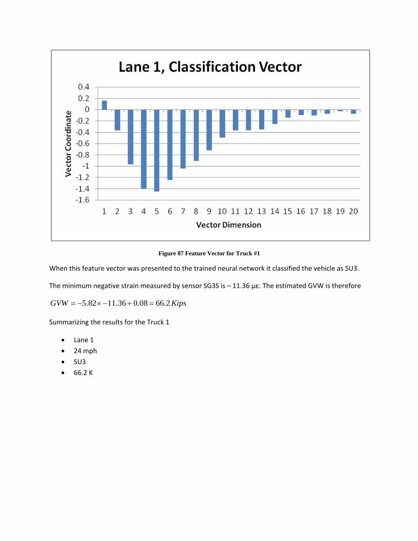
Figure 87 Feature Vector for Truck #1
When this feature vector was presented to the trained neural network it classified the vehicle as SU3.
The minimum negative strain measured by sensor SG3S is – 11.36 με. The estimated GVW is therefore
KipsGVW 2.6608.036.1182.5 =+−×−=
Summarizing the results for the Truck 1
• Lane 1 • 24 mph • SU3 • 66.2 K
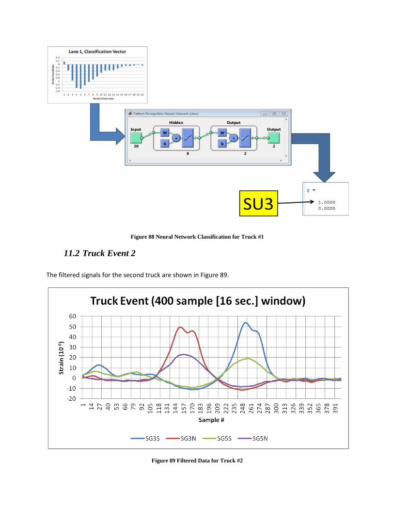
Figure 88 Neural Network Classification for Truck #1
11.2 Truck Event 2
The filtered signals for the second truck are shown in Figure 89.
Figure 89 Filtered Data for Truck #2
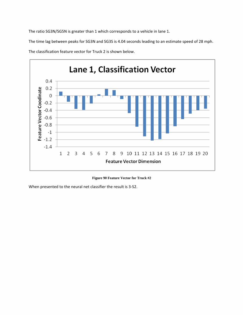
The ratio SG3N/SG5N is greater than 1 which corresponds to a vehicle in lane 1.
The time lag between peaks for SG3N and SG3S is 4.04 seconds leading to an estimate speed of 28 mph.
The classification feature vector for Truck 2 is shown below.
Figure 90 Feature Vector for Truck #2
When presented to the neural net classifier the result is 3-S2.

Figure 91 Neural Network Classification for Truck #2
The gross vehicle weight for a 3-S2 vehicle in lane 1 is calculated to be:
KipsGVW 9.6718.0)06.11(16.6 =−−×−=
Summarizing for Truck 2
• Lane 1 • 28 mph • 3-S2 • 67.9 K
11.3 Truck Event 3
The filtered response for the third truck is shown in Figure 92. It is noted that the amplitude for the downstream peak is much lower than expected.
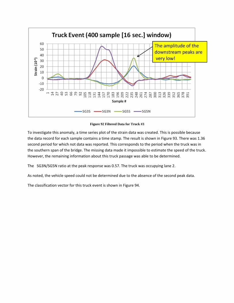
Figure 92 Filtered Data for Truck #3
To investigate this anomaly, a time series plot of the strain data was created. This is possible because the data record for each sample contains a time stamp. The result is shown in Figure 93. There was 1.36 second period for which not data was reported. This corresponds to the period when the truck was in the southern span of the bridge. The missing data made it impossible to estimate the speed of the truck. However, the remaining information about this truck passage was able to be determined.
The SG3N/SG5N ratio at the peak response was 0.57. The truck was occupying lane 2.
As noted, the vehicle speed could not be determined due to the absence of the second peak data.
The classification vector for this truck event is shown in Figure 94.
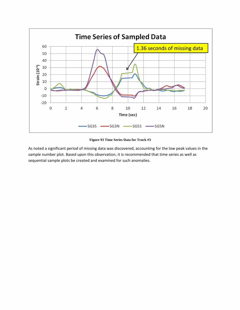
Figure 93 Time Series Data for Truck #3
As noted a significant period of missing data was discovered, accounting for the low peak values in the sample number plot. Based upon this observation, it is recommended that time series as well as sequential sample plots be created and examined for such anomalies.
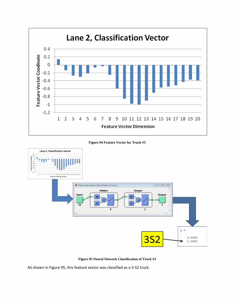
Figure 94 Feature Vector for Truck #3
Figure 95 Neural Network Classification of Truck #3
AS shown in Figure 95, this feature vector was classified as a 3-S2 truck.
The GVW of this truck was determined using the appropriate regression equation.
KipsGVW 8.5821.0)73.13(27.4 =+−×−=
Summarizing for Truck 3
• Lane 2 • unknown • 3-S2 • 58.8 K
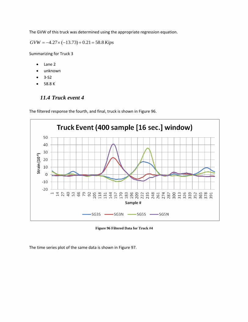
11.4 Truck event 4
The filtered response the fourth, and final, truck is shown in Figure 96.
Figure 96 Filtered Data for Truck #4
The time series plot of the same data is shown in Figure 97.
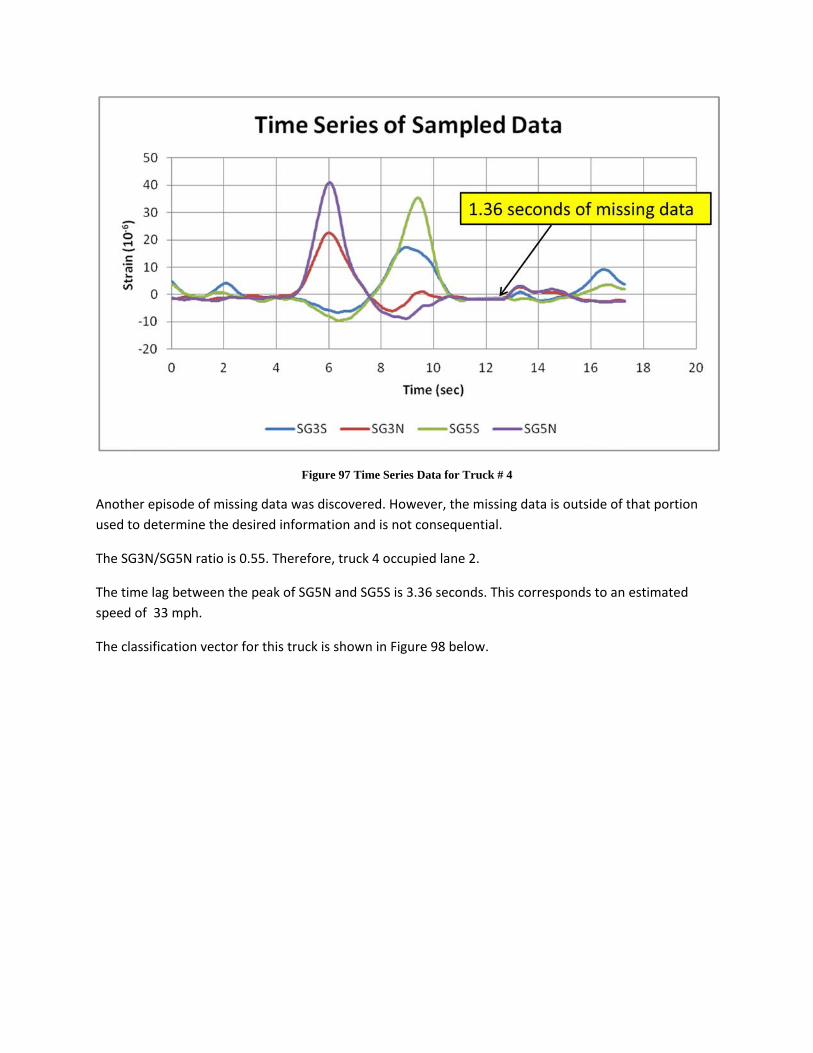
Figure 97 Time Series Data for Truck # 4
Another episode of missing data was discovered. However, the missing data is outside of that portion used to determine the desired information and is not consequential.
The SG3N/SG5N ratio is 0.55. Therefore, truck 4 occupied lane 2.
The time lag between the peak of SG5N and SG5S is 3.36 seconds. This corresponds to an estimated speed of 33 mph.
The classification vector for this truck is shown in Figure 98 below.
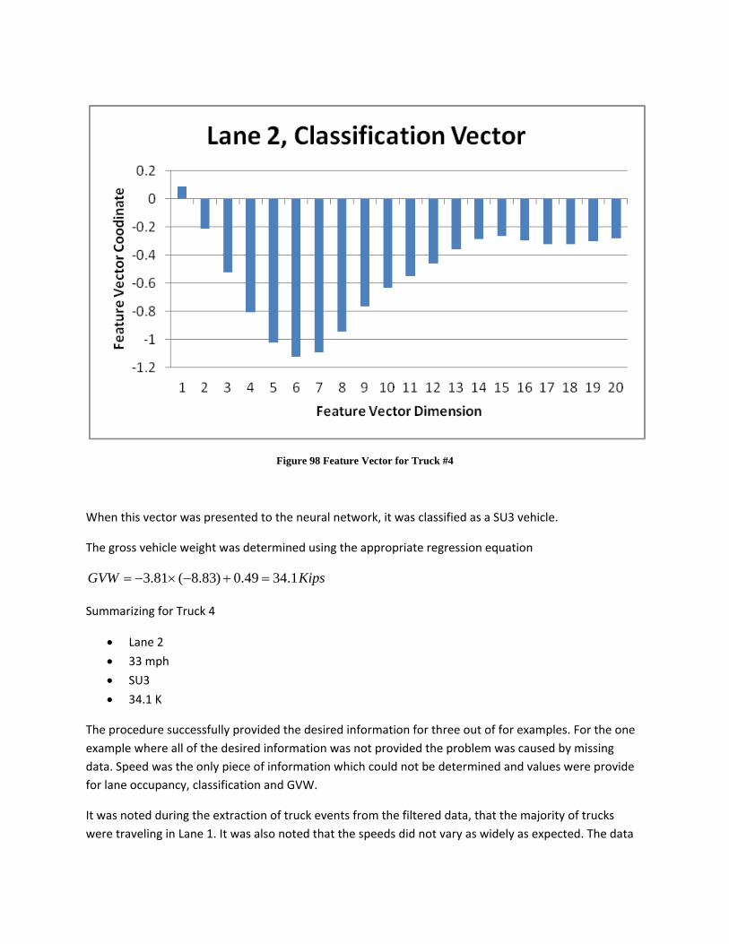
Figure 98 Feature Vector for Truck #4
When this vector was presented to the neural network, it was classified as a SU3 vehicle.
The gross vehicle weight was determined using the appropriate regression equation
KipsGVW 1.3449.0)83.8(81.3 =+−×−=
Summarizing for Truck 4
• Lane 2 • 33 mph • SU3 • 34.1 K
The procedure successfully provided the desired information for three out of for examples. For the one example where all of the desired information was not provided the problem was caused by missing data. Speed was the only piece of information which could not be determined and values were provide for lane occupancy, classification and GVW.
It was noted during the extraction of truck events from the filtered data, that the majority of trucks were traveling in Lane 1. It was also noted that the speeds did not vary as widely as expected. The data
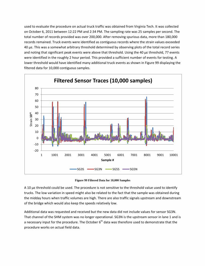
used to evaluate the procedure on actual truck traffic was obtained from Virginia Tech. It was collected on October 6, 2011 between 12:22 PM and 2:34 PM. The sampling rate was 25 samples per second. The total number of records provided was over 200,000. After removing spurious data, more than 180,000 records remained. Truck events were identified as contiguous records where the strain values exceeded 40 με. This was a somewhat arbitrary threshold determined by observing plots of the total record series and noting that significant peak events were above that threshold. Using the 40 με threshold, 77 events were identified in the roughly 2 hour period. This provided a sufficient number of events for testing. A lower threshold would have identified many additional truck events as shown in Figure 99 displaying the filtered data for 10,000 contiguous samples.
Figure 99 Filtered Data for 10,000 Samples
A 10 με threshold could be used. The procedure is not sensitive to the threshold value used to identify trucks. The low variation in speed might also be related to the fact that the sample was obtained during the midday hours when traffic volumes are high. There are also traffic signals upstream and downstream of the bridge which would also keep the speeds relatively low.
Additional data was requested and received but the new data did not include values for sensor SG3N. That channel of the SHM system was no longer operational. SG3N is the upstream sensor in lane 1 and is a necessary input for the procedure. The October 6th data was therefore used to demonstrate that the procedure works on actual field data.
-20
-10
0
10
20
30
40
50
60
70
80
1 1001 2001 3001 4001 5001 6001 7001 8001 9001 10001
Stra
in 1
0-6
Sample #
Filtered Sensor Traces (10,000 samples)
SG3S SG3N SG5S SG5N
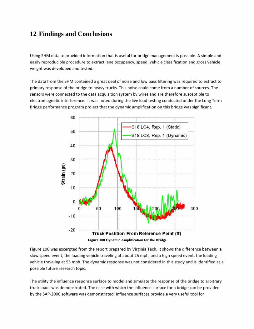
12 Findings and Conclusions
Using SHM data to provided information that is useful for bridge management is possible. A simple and easily reproducible procedure to extract lane occupancy, speed, vehicle classification and gross vehicle weight was developed and tested. The data from the SHM contained a great deal of noise and low pass filtering was required to extract to primary response of the bridge to heavy trucks. This noise could come from a number of sources. The sensors were connected to the data acquisition system by wires and are therefore susceptible to electromagnetic interference. It was noted during the live load testing conducted under the Long Term Bridge performance program project that the dynamic amplification on this bridge was significant.
Figure 100 Dynamic Amplification for the Bridge
Figure 100 was excerpted from the report prepared by Virginia Tech. It shows the difference between a slow speed event, the loading vehicle traveling at about 25 mph, and a high speed event, the loading vehicle traveling at 55 mph. The dynamic response was not considered in this study and is identified as a possible future research topic. The utility the influence response surface to model and simulate the response of the bridge to arbitrary truck loads was demonstrated. The ease with which the influence surface for a bridge can be provided by the SAP-2000 software was demonstrated. Influence surfaces provide a very useful tool for

determining the response of a bridge to arbitrary loadings. This is also an area where future research is suggested but with a focus on load rating and load permitting. The predominance of heavy truck traffic in lane 1 was noted on this bridge. It is unknown whether this is a general characteristic of all bridges on all roads or whether this is a characteristic of this bridge given that there is an on-ramp to Interstate highway 66 located immediately south of this bridge. The reliability of the SHM, i.e. the availability of the input data, was not very good. Although the procedure developed in this study is able to extract useful information for bridge management, it relies upon the data provided by the SHM. There were problems with missing data, non-functioning channels and overall system operation during this study.
13 Future research
Overall, this study was very successful in that it was able to provide useful information for bridge management. However, there are several areas where additional or follow-on research is suggested. The procedure developed under this study worked very well for individual truck events. These truck events were identified as occurring when a particular strain threshold was exceeded. In the majority of cases these threshold exceeding events were due to the passage of a single truck. In a few instance, the signals show a pattern which suggests the presence of multiple trucks, as shown in Figure 101.
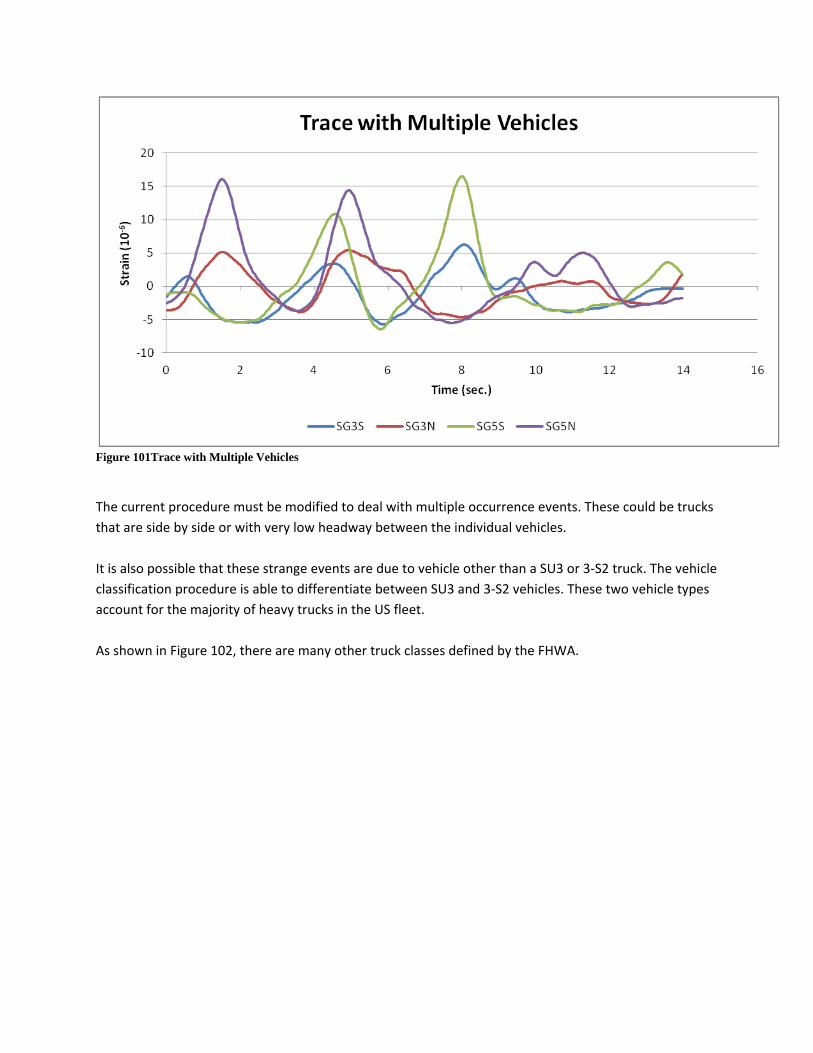
Figure 101Trace with Multiple Vehicles
The current procedure must be modified to deal with multiple occurrence events. These could be trucks that are side by side or with very low headway between the individual vehicles. It is also possible that these strange events are due to vehicle other than a SU3 or 3-S2 truck. The vehicle classification procedure is able to differentiate between SU3 and 3-S2 vehicles. These two vehicle types account for the majority of heavy trucks in the US fleet. As shown in Figure 102, there are many other truck classes defined by the FHWA.
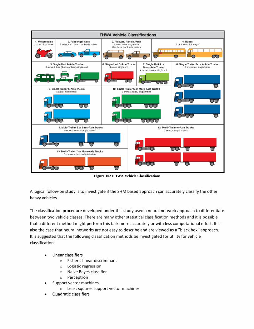
Figure 102 FHWA Vehicle Classifications
A logical follow-on study is to investigate if the SHM based approach can accurately classify the other heavy vehicles. The classification procedure developed under this study used a neural network approach to differentiate between two vehicle classes. There are many other statistical classification methods and it is possible that a different method might perform this task more accurately or with less computational effort. It is also the case that neural networks are not easy to describe and are viewed as a ”black box” approach. It is suggested that the following classification methods be investigated for utility for vehicle classification.
• Linear classifiers o Fisher's linear discriminant o Logistic regression o Naive Bayes classifier o Perceptron
• Support vector machines o Least squares support vector machines
• Quadratic classifiers

• Kernel estimation • k-nearest neighbor • Decision trees • Bayesian networks • Hidden Markov models • Learning vector quantization
The procedure developed for this study is very much tied to the specific bridge which was instrumented. The speed, vehicle classification and GVW estimation procedures all made use of features and characteristics of the influence surface for this bridge. In particular, the fact that the bridge was a two span continuous structure was very much exploited. Another follow-on study is to investigate how transferable the procedure is to other bridge types.
As noted, the procedures developed did not account for the dynamic behavior of the bridge. Another research study could be an investigation of the significance of bridge dynamics on the ability to extract useful bridge management information from SHM data. A final future research study would be to develop a general approach to the use of influence surfaces for bridge load rating and permitting. While SAP-2000 provides a useful capability for the generation of influence surfaces for a specific bridge, this is not unique to SAP-2000. Any general purpose finite element modeling package can produce an influence surface. However, these influence surfaces require large file sizes to store. It is suggested to investigate how influence surfaces might be created for any bridge in an efficient manner. As a part of this study, it is suggested to also investigate low fidelity surfaces, those with minimal number of interpolation points. Also, investigate how a response surface could be compactly stored, either with a compression approach or parameterization.

14 References
Alampalli, S., Ettouney, M., (2008), “Role of Structural Health Monitoring in Bridge Security,” Bridge Structures: Assessment, Design, and Construction, 4(3-4):143-154. AASHTO, (2005), “Guide Manual for Condition Evaluation and Load and Resistance Factor Rating (LRFR) of Highway Bridges,” American Association of State Highway and Transportation Officials, Washington DC AASHTO, (2002), AASHTO Standard Specifications for Highway Bridges, 17th Edition, HB-17. American Association of State Highway and Transportation Officials, Washington, DC. Bell, E.S., Sipple, J.D., Lefebvre, P.J., Phelps, J.E., Brenner, B., Sanayei, M., (2010), “Instrumentation, Modeling and Monitoring of a Concrete Bridge from Construction through Service,” Transportation Research Board 89th Annual Meeting, Paper #10-1861. Carden, E.P., Fanning, P., (2004), “Vibration Based Condition Monitoring: A Review,” International Journal of Structural Health Monitoring, 3(4):355-377. Carkhuff, B., Cain, R., (2003), “Corrosion Sensors for Concrete Bridges,” IEEE Instrumentation and Measurement Magazine, 6(2): 19-24. Casas, J.R., Cruz, P.J.S., (2003), “Fiber Optic Sensors for Bridge Monitoring,” Journal of Bridge Engineering, 8:362-373. Chacón, R., Guzmán, F., Mirambell, E., Real, E., Oñate, E., (2009), “Wireless Sensor Networks for Strain Monitoring during Steel Bridges Launching,” Structural Health Monitoring, 8(3):195-205. Chang, P.C., Flatau, A., Liu, S.C., (2003), “Review Paper: Health Monitoring of Civil Infrastructure,” International Journal of Structural Health Monitoring, 2(3):257-267. Chung, W., Sotelino, E.D., (2005), “Three-Dimensional Finite Element Modeling of Composite Girder Bridges,” Journal of Engineering Structures, 28:63-71.
Conte, J.P., He, X., Moaveni, B., Masri, S.F., Caffrey, J.P., Wahbeh, M., Tasbihgoo, F., Whang, D.H., Elgamal, A., 2008, “Dynamic testing of Alfred Zampa Memorial Bridge,” Journal of Structural Engineering, 134(6):1006-1015. Cook, R.D., (1995), Finite Element Modeling for Stress Analysis, John Wiley and Sons, Inc. (1 ed.), NY. Cross, B., Vaughn, B., Panahshahi, N., Petermeier, D., Siow, Y.S., Domagalski, T., (2009), “Analytical and Experimental Investigation of Bridge Girder Shear Distribution Factors,” Journal of Bridge Engineering, 14(3):154-163.

DeWolf, J., (2009), “Structural Health Monitoring of Three Bridges in Connecticut,” Transportation Research Board 88th Annual Meeting. DeWolf, J., Lauzon, R.G., Culmo, M.P., (2002), “Monitoring Bridge Performance,” International Journal of Structural Health Monitoring, 10:129-138. Doebling, S.W., Farrar, C.R., Prime, M.B., (1998), “A Summary Review of Vibration-based Damage Identification Methods,” The Shock and Vibration Digest, 30(2):91-105. Doherty, J.E., (1987), “Nondestructive evaluation,” in Handbook on Experimental Mechanics, A.S. Kobayashi, ed., Society for Experimental Mechanics. Faber, M.H., Val, D.V., Stewart, M.G., (2000), “Proof Load Testing for Bridge Assessment and Upgrading,” Engineering Structures, 22(12):1677-1689. Feeley, Katherine (2010), Modeling a Steel Composite Bridge with a Non-Uniform Section Using SAP2000 MS Thesis, University of Virginia Friswell, M.I., Mottershead, J.E., (1995), Solid Mechanics and its Applications: Finite Element Model Updating in Structural Dynamics, Kluwer Academic Publishers, Norwell, MA. Halfawy, M.R., Wipf, T., Wood, D., Abu-Hawash, A., Phares, B., (2002), “Bridge Load Rating Using an Integrated Load Testing and Finite Element Analysis Approach: A Case Study,” Proceedings, Annual Conference - Canadian Society for Civil Engineering, 2002: 1371-1379. Hoppe, E.J., Bagnall, T.M., (2008), “Performance of a Skewed Semi-Integral Bridge: Volume 1: Field Monitoring,” Virginia Transportation Research Council, VTRC 08-R20, Hunt, V., Helmicki, A., and Swanson, J., (2005), “Instrumentation and Monitoring of the U.S. Grant Bridge,” Proceedings of ASNT Structural Materials Technology VI: An NDT Conference, Columbus, OH, October, 2005. Jaramilla, B., Huo, S., (2005), “Looking to Load and Resistance Factor Rating,” Public Roads, 69(1), http://www.tfhrc.gov/pubrds. Ko, J.M., Ni, Y.Q., (2005), “Technology Development in Structural Health Monitoring of Large Scale Bridges,” Engineering Structures, 27:1715-1725. Liu, C., Olund, J., Cardini, A., D’Attilio, P., Feldblum, E., DeWolf, J., (2008), “Structural Health Monitoring of Bridges in the State of Connecticut,” Earthquake Engineering and Engineering Vibrations, 7(4):427-437. Lucas, J., Cousins, T., Brown, M.C., (2006), “Structural Load Testing and Flexure Analysis of the Route 701 Bridge in Louisa County, Virginia: Supplemental Report,” Report VTRC 06-R14 Mabsout, M.E., Tarhini, K.M., Frederick, G.R., Tayar, C. (1997). “Finite-Element Analysis of Steel Girder Highway Bridges,” Journal of Bridge Engineering, 2(3):83-87.

Mehrani, E., Ayoub, A., (2006), “Remote health monitoring of the first smart bridge in Florida,” Proceedings of the Structures Congress and Exposition, 2006:90 Mehrani, E., Ayoub, A., Ayoub, A. (2009), “Evaluation of Fiber Optic Sensors for Remote Health Monitoring of Bridge Structures,” Materials and Structures, 42(2):183-199. Morris, A., (2008), A Practical Guide to Reliable Finite Element Modelling, John Wiley & Sons, Ltd. NCHRP, (1998), “Manual for Bridge Rating Through Load Testing,” National Cooperative Highway Research Program Research Results Digest NCHRP No. 234. Ou, J., (2005), “Some Recent Advances of Intelligent Health Monitoring Systems for Civil Infrastructure in HIT,” Fundamental problems of optoelectronics and microelectronics II: 13-16 September, 2004, Khabarovsk, Russia, 5851:147-162. Ozgur, C., (2007), “Behavior and Analysis of a Curved and Skewed I-Girder Bridge,” Master of Science Thesis, Georgia Institute of Technology, Ruth, N., Kangas, S., Mittal, S., Helmicki, A., Swanson, J., and Hunt, V., (2005), “Field Testing and Analysis of 40 Steel Stringer Bridges,” Proceedings of ASNT Structural Materials Technology VI: An NDT Conference, Columbus, OH. Shehata, E., Rizkalla, S., (1999), “Intelligent Sensing for Innovative Bridges,” Journal of Intelligent Material Systems and Structures, 10:304-313. Texas Instruments, (2009), Retrieved December 8, 2009, from Texas Instruments, Inc. http://www.ti.com. Tzamtzis A.D., (2003). “Finite Element Modelling of Cracks and Joints in Discontinuous Structural Systems,” Proceedings of the 16th ASCE Engineering Mechanics Conference, University of Washington, Missouri, USA. VTRC (2010), Virginia Pilot Bridge Live Load Test Summary Preliminary Work product from VTRC, March 30, 2010. Walther, R.A., Chase, S.B., (2006), “Condition Assessment of Highway Structures: Past, Present, and Future,” Proc. of 2006 Transportation Research Board, No. P06-1360. Whelan, M.J., Janoyan, K.D., (2009), “Design of a Robust, High-rate Wireless Sensor Network for Static and Dynamic Structural Monitoring,” Journal of Intelligent Material Systems and Structures, 20(7):849-863. Wong, K.Y., (2007), “Design of a Structural Health Monitoring System for Long-Span Bridges,” Structure and Infrastructure Engineering, 3(2):169-185. Zwolski, J., Bién, J. (2008), “Modern Technologies in Bridge Monitoring,” Proceedings of the Fourth European Workshop in Structural Health Monitoring, 201-210.

14.1 Extended Bibliography
Ahn, J-H, Sim, C., Jeong, Y-J, Kim, S-H., (2009), “Fatigue Behavior and Statistical Evaluation of the Stress Category for a Steel-Concrete Composite Bridge Deck,” Journal of Constructional Steel Research, 65(2):373-385. Bell, E.S., (2008), “Bridge Condition Assessment Framework Integrating Structural Health Monitoring and Intelligent Transportation Technology,” Transportation Research Board 87th Annual Meeting. Bessho, K. Nishikawa, Y., Takada, Y., Sakano, M., (2009), “Fatigue damage of an urban expressway steel girder bridge constructed in 1964,” Science and technology reports of Kansai University, 51:55-59. Brownjohn, J.M.W., (2007), “Structural Health Monitoring of Civil Infrastructure,” Philosophical Transactions. Series A, Mathematical, Physical, and Engineering Sciences, 365(1851):589-622. Clash, T.W., Delaney, J.B., (2000), “New York State’s Approach to Asset Management: A Case Study,” Transportation Research Record, (1729): 35-41. Dicdican, R.Y., Haimes, Y.Y., Lambert, J.H., (2004), “Risk-Based Asset Management Methodology for Highway Infrastructure Systems,” Virginia Transportation Research Council, VTRC 04-CR11, Doebling, S.W., Farrar, C.R., Prime, M.B., Shevitz, D.W., (1996), “Damage Identification and Health Monitoring of Structural and Mechanical Systems from Changes in their Vibration Characteristics: A Literature Review,” Technical Report No. LA-13070-MS, Los Alamos National Laboratory, Los Alamos, NM. Federal Highway Administration (FHWA), Office of Asset Management (2007), “Asset Management Overview,” FHWA-IF-08-008, U.S. Department of Transportation, http://www.fhwa.dot.gov/asset/if08008/assetmgmt_overview.pdf. Federal Highway Administration (FWHA) (1999), “Asset Management Primer,” Director M. Bloom US Department of Transportation, FHWA, Office of Asset Management. Frýba, L., Pirner, M., (2001), “Load Tests and Modal Analysis of Bridges,” Engineering Structures, 23: 102-109. Gangone, M.V., Whelan, M.J., Janovan, K.D., (2008), “Structural Health Management of Concrete Structures Using Wireless Sensors,” American Concrete Institute, 125-135. Godzwon, G., (2004), “Bridge Asset Management: Planning and Preservation,” Government Engineering, 13(1): Harrison, R., Gurenich, D., Robert, W., (2006), “An Approach to Integrating Bridge and Other Asset Management Analyses,” Bridge Maintenance, Safety, Management, Life-Cycle Performance and Cost, 729-730.

Hegazy, R., Elbeltagi, E., El-Behairy, H., (2004), “Bridge Deck Management System with Integrated Life-Cycle Cost Optimization,” Transportation Research Record: Journal of the Transportation Research Board, No. 1866, TRB, National Research Council, Washington, D.C., 2004, pp. 44-50. Hoppe, E.J., (2006), “Field Measurements on Skewed Semi-Integral Bridge with Elastic Inclusion: Instrumentation Report,” Virginia Transportation Research Council, VTRC 06-R35 Hou, T.-C., Lynch, J.P., (2006), “Rapid-to-Deploy Wireless Monitoring Systems for Static and Dynamic Load Testing of Bridges: Validation on the Grove Street Bridge,” Proceedings of the SPIE - The International Society for Optical Engineering, 6178:61780D. Jivacate, I., Najafi, F.T., (2003), “The Current Status of Bridge Management Systems,” Annual Conference of the Canadian Society for Civil Engineering, GCG-285, 1-10. Jurkiewiez, B., (2009), “Static and Cyclic Behaviour of a Steel-Concrete Composite Beam with Horizontal Shear Connections,” Journal of Constructional Steel Research, 65(12):2207-2216. Laboratoire Central des Ponts et Chaussees (LCPC), (2001), “Weight-in-motion of Axles and Vehicles for Europe (WAVE) – General Report” RTD Project, RO-96-SC, 403. Lwin, M.M., (2006), “The Important Roles of Bridge Maintenance and Management on Transportation Safety and Efficiency,” Bridge Maintenance, Safety, Management, Life-Cycle Performance and Cost, Taylor & Francis Group, London, 47-51. Minchin Jr., R.E., Zayed, R., Boyd, A.J., Mendoza, M., (2006), “Best Practices of Bridge System Management – A Synthesis,” Journal of Management in Engineering, 186-195. Mosallam, A., Miraj, R., Abdi, R., (2009), “Diagnostic/Prognostic health monitoring system and evaluation of a composite bridge,” Smart Structures and Systems, 5(4):397-413. NCHRP, (2009), “Bridge Management Systems for Transportation Agency Decision Making – A Synthesis of highway practice,” National Cooperative Highway Research Program (NCHRP), NCHRP Synthesis 397, Transportation Research Board, 2009. (Consultants: M.J. Markow, W.A. Hyman) Nevling, D., Linzell, D., Laman, J., (2006), “Examination of Level of Analysis Accuracy for Curved I-Girder Bridges through Comparisons to Field Data,” Journal of Bridge Engineering, 11(2): 160-168. Nowak, A.S., Kim, S., Szerszen, M.M., (1999), “Dynamic Loads for Steel Girder Bridges,” Proceedings of the International Modal Analysis Conference & Exhibit, 1:731-737. O’Brien, E.J., Rattigan, P., González, A., Dowling, J., Žnidarič, A. (2009), “Characteristic Dynamic Traffic Load Effects in Bridges,” Engineering Structures, 31(7):1607-1612. Olson, C.C., Overbey, L.A., Todd, M.D., (2009), “The Effect of Detection Feature Type on Excitations Bred for Active Sensing in Structural Health Monitoring,” Journal of Intelligent Material Systems and Structures, 20:1307-1327.

Peters, M., (2000) “Transportation Asset Management” Powerpoint presentation, Arizona Department of Transportation, “AASHTO National Initiative” AASHTO Spring Meeting. Saraf, V., Nowak, A.S., (1998), “Proof load testing of deteriorated steel girder bridges,” Journal of Bridge Engineering, 3(2):82-89. Sidawi, S., Shehata, E., (2008), “Using Infrastructure Health Monitoring (IHM) to Assess the Impact of Climate Change on Civil Infrastructure,” 2008 Annual Conference of the Transportation Association of Canada. Sleiman, S., (2009), “Bridging the Visual Gap: Tobin Bridge Goes Beyond Visual Inspections with Electronic Health Monitoring,” Roads and Bridges, 47(2):50-53. Sohn, H., Farrar, C.R., Hemez, F.M., Czarnecki, J.J., Shunk, D.D., Stinemates, D.W., and Nadler, B.R., (2004), “A Review of Structural Health Monitoring Literature: 1996-2001,” Technical Report No. LA-13976-MS, Los Alamos National Laboratory, Los Alamos, NM. Sumitro, S., Wang, M.L., (2005), “Sustainable Structural Health Monitoring System,” Structural Control Health Monitoring, 12:445-467. Sun, X., Zhang, Z., Wang, R., Wang, X., Chapman, J., (2004), “Analysis of Past National Bridge Inventory Ratings for Predicting Bridge System Preservation Needs,” Transportation Research Record: Journal of the Transportation Research Board, No. 1866, TRB, National Research Council, Washington, D.C., 2004, pp. 36-43. Tserng, H.P., Chung, C-L., (2007), “Health Assessment and Maintenance Strategy for Bridge Management Systems: Lessons Learned in Taiwan,” Journal of Infrastructure Systems, 13(3): 235-246. Wang, Y., Lynch, J.P., Law, K.H., (2007), “A Wireless Structural Health Monitoring System with Multithreaded Sensing Devices: Design and Validation,” Structure and Infrastructure Engineering, 3(2):103-120. Yao, J.T.P., Wong, F.S., “Structural Health Monitoring and Symptom-Based Reliability,” Life-Cycle Cost Analysis and Design of Civil Infrastructure Systems, 314-320.

15 Appendices
MATLAB Code %InfluenceInterp1 - Creates matrices of influence surface data for sensor % SG3N on the Route 15 Bridge. % This m-file will assemble influence data from an excel spreadsheet exported % From SAP-2000 model into matrices of data and export the variables to a % mat file for use in subsequent functions. % A very similar program was used for sensors SG3S,SG5N and SG5S % % Author: Katherine Feeley 5 modified by Steven Chase % email: [email protected] % April 2010; Last revision: July 2012 %------------- BEGIN CODE -------------- SheetName = 'SG3N'; X = xlsread('InfluenceTable.xlsx',SheetName,'A2:A7876'); Y = xlsread('InfluenceTable.xlsx',SheetName,'B2:B7876'); V = xlsread('InfluenceTable.xlsx',SheetName,'C2:C7876'); save('SG3Nvalues.mat','X','Y','V'); %Saves variables to -mat file %------------- END OF CODE --------------
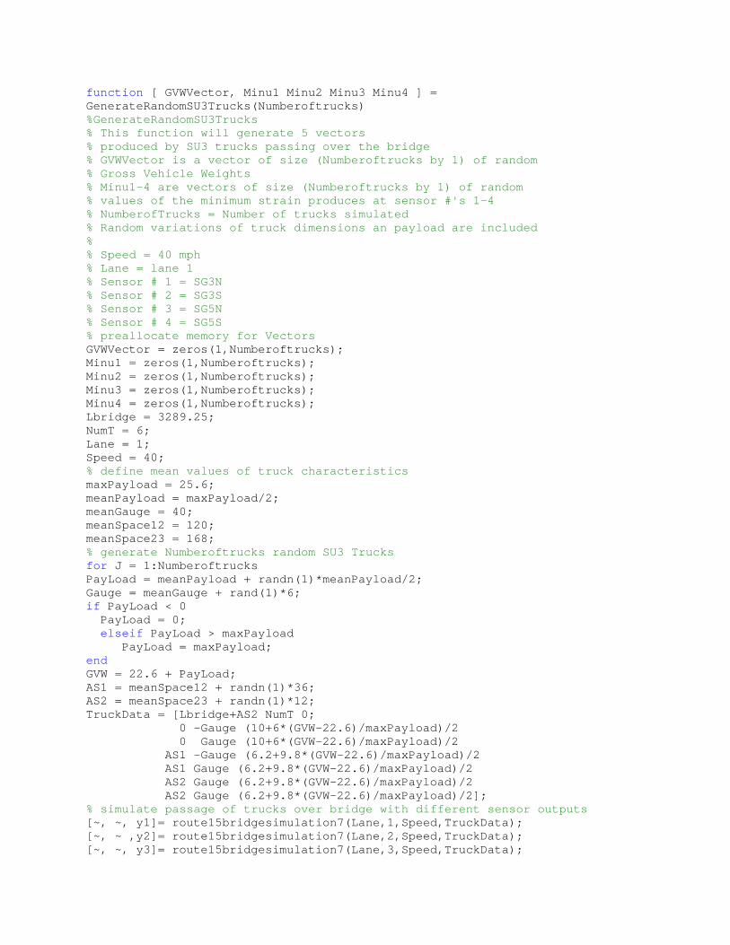
function [ GVWVector, Minu1 Minu2 Minu3 Minu4 ] = GenerateRandomSU3Trucks(Numberoftrucks) %GenerateRandomSU3Trucks % This function will generate 5 vectors % produced by SU3 trucks passing over the bridge % GVWVector is a vector of size (Numberoftrucks by 1) of random % Gross Vehicle Weights % Minu1-4 are vectors of size (Numberoftrucks by 1) of random % values of the minimum strain produces at sensor #'s 1-4 % NumberofTrucks = Number of trucks simulated % Random variations of truck dimensions an payload are included % % Speed = 40 mph % Lane = lane 1 % Sensor # 1 = SG3N % Sensor # 2 = SG3S % Sensor # 3 = SG5N % Sensor # 4 = SG5S % preallocate memory for Vectors GVWVector = zeros(1,Numberoftrucks); Minu1 = zeros(1,Numberoftrucks); Minu2 = zeros(1,Numberoftrucks); Minu3 = zeros(1,Numberoftrucks); Minu4 = zeros(1,Numberoftrucks); Lbridge = 3289.25; NumT = 6; Lane = 1; Speed = 40; % define mean values of truck characteristics maxPayload = 25.6; meanPayload = maxPayload/2; meanGauge = 40; meanSpace12 = 120; meanSpace23 = 168; % generate Numberoftrucks random SU3 Trucks for J = 1:Numberoftrucks PayLoad = meanPayload + randn(1)*meanPayload/2; Gauge = meanGauge + rand(1)*6; if PayLoad < 0 PayLoad = 0; elseif PayLoad > maxPayload PayLoad = maxPayload; end GVW = 22.6 + PayLoad; AS1 = meanSpace12 + randn(1)*36; AS2 = meanSpace23 + randn(1)*12; TruckData = [Lbridge+AS2 NumT 0; 0 -Gauge (10+6*(GVW-22.6)/maxPayload)/2 0 Gauge (10+6*(GVW-22.6)/maxPayload)/2 AS1 -Gauge (6.2+9.8*(GVW-22.6)/maxPayload)/2 AS1 Gauge (6.2+9.8*(GVW-22.6)/maxPayload)/2 AS2 Gauge (6.2+9.8*(GVW-22.6)/maxPayload)/2 AS2 Gauge (6.2+9.8*(GVW-22.6)/maxPayload)/2]; % simulate passage of trucks over bridge with different sensor outputs [~, ~, y1]= route15bridgesimulation7(Lane,1,Speed,TruckData); [~, ~ ,y2]= route15bridgesimulation7(Lane,2,Speed,TruckData); [~, ~, y3]= route15bridgesimulation7(Lane,3,Speed,TruckData);
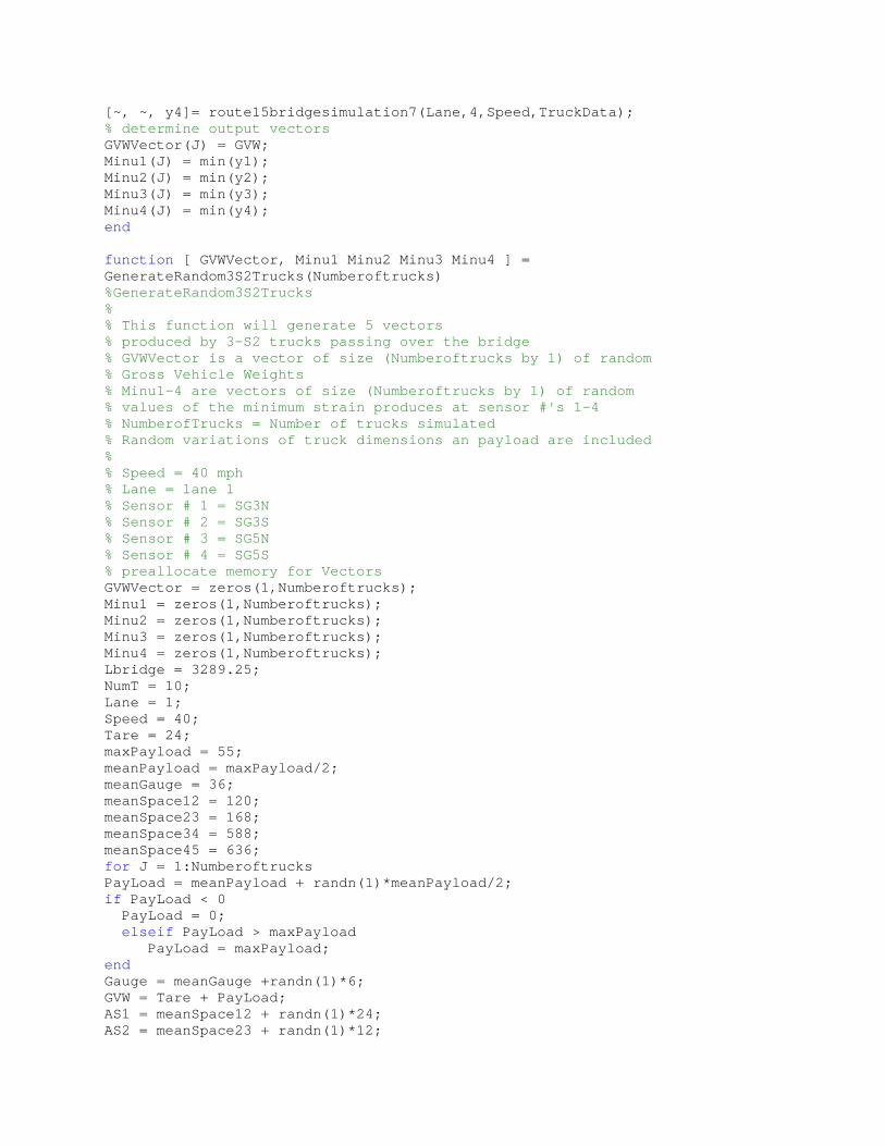
[~, ~, y4]= route15bridgesimulation7(Lane,4,Speed,TruckData); % determine output vectors GVWVector(J) = GVW; Minu1(J) = min(y1); Minu2(J) = min(y2); Minu3(J) = min(y3); Minu4(J) = min(y4); end function [ GVWVector, Minu1 Minu2 Minu3 Minu4 ] = GenerateRandom3S2Trucks(Numberoftrucks) %GenerateRandom3S2Trucks % % This function will generate 5 vectors % produced by 3-S2 trucks passing over the bridge % GVWVector is a vector of size (Numberoftrucks by 1) of random % Gross Vehicle Weights % Minu1-4 are vectors of size (Numberoftrucks by 1) of random % values of the minimum strain produces at sensor #'s 1-4 % NumberofTrucks = Number of trucks simulated % Random variations of truck dimensions an payload are included % % Speed = 40 mph % Lane = lane 1 % Sensor # 1 = SG3N % Sensor # 2 = SG3S % Sensor # 3 = SG5N % Sensor # 4 = SG5S % preallocate memory for Vectors GVWVector = zeros(1,Numberoftrucks); Minu1 = zeros(1,Numberoftrucks); Minu2 = zeros(1,Numberoftrucks); Minu3 = zeros(1,Numberoftrucks); Minu4 = zeros(1,Numberoftrucks); Lbridge = 3289.25; NumT = 10; Lane = 1; Speed = 40; Tare = 24; maxPayload = 55; meanPayload = maxPayload/2; meanGauge = 36; meanSpace12 = 120; meanSpace23 = 168; meanSpace34 = 588; meanSpace45 = 636; for J = 1:Numberoftrucks PayLoad = meanPayload + randn(1)*meanPayload/2; if PayLoad < 0 PayLoad = 0; elseif PayLoad > maxPayload PayLoad = maxPayload; end Gauge = meanGauge +randn(1)*6; GVW = Tare + PayLoad; AS1 = meanSpace12 + randn(1)*24; AS2 = meanSpace23 + randn(1)*12;
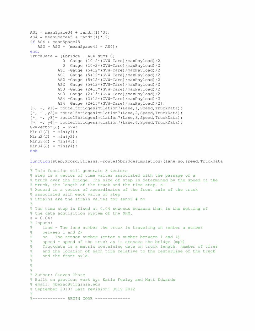
AS3 = meanSpace34 + randn(1)*36; AS4 = meanSpace45 + randn(1)*12; if AS4 > meanSpace45 AS3 = AS3 - (meanSpace45 - AS4); end; TruckData = [Lbridge + AS4 NumT 0; 0 -Gauge (10+2*(GVW-Tare)/maxPayload)/2 0 Gauge (10+2*(GVW-Tare)/maxPayload)/2 AS1 -Gauge (5+12*(GVW-Tare)/maxPayload)/2 AS1 Gauge (5+12*(GVW-Tare)/maxPayload)/2 AS2 -Gauge (5+12*(GVW-Tare)/maxPayload)/2 AS2 Gauge (5+12*(GVW-Tare)/maxPayload)/2 AS3 -Gauge (2+15*(GVW-Tare)/maxPayload)/2 AS3 Gauge (2+15*(GVW-Tare)/maxPayload)/2 AS4 -Gauge (2+15*(GVW-Tare)/maxPayload)/2 AS4 Gauge (2+15*(GVW-Tare)/maxPayload)/2]; [~, ~, y1]= route15bridgesimulation7(Lane,1,Speed,TruckData); [~, ~ ,y2]= route15bridgesimulation7(Lane,2,Speed,TruckData); [~, ~, y3]= route15bridgesimulation7(Lane,3,Speed,TruckData); [~, ~, y4]= route15bridgesimulation7(Lane,4,Speed,TruckData); GVWVector(J) = GVW; Minu1(J) = min(y1); Minu2(J) = min(y2); Minu3(J) = min(y3); Minu4(J) = min(y4); end function[step,Xcord,Strains]=route15bridgesimulation7(lane,no,speed,Truckdata) % This function will generate 3 vectors % step is a vector of time values associated with the passage of a % truck over the bridge. The size of step is determined by the speed of the % truck, the length of the truck and the time step, s. % Xcoord is a vector of xcoordinates of the front axle of the truck % associated with eack value of step % Strains are the strain values for senor # no % % The time step is fixed at 0.04 seconds because that is the setting of % the data acquisition system of the SHM. s = 0.04; % Inputs: % lane - The lane number the truck is traveling on (enter a number % between 1 and 2) % no - The sensor number (enter a number between 1 and 4) % speed - speed of the truck as it crosses the bridge (mph) % Truckdata is a matrix containing data on truck length, number of tires % and the location of each tire relative to the centerline of the truck % and the front axle. % % % % Author: Steven Chase % Built on previous work by: Katie Feeley and Matt Edwards % email: [email protected] % September 2010; Last revision: July-2012 % %------------- BEGIN CODE --------------
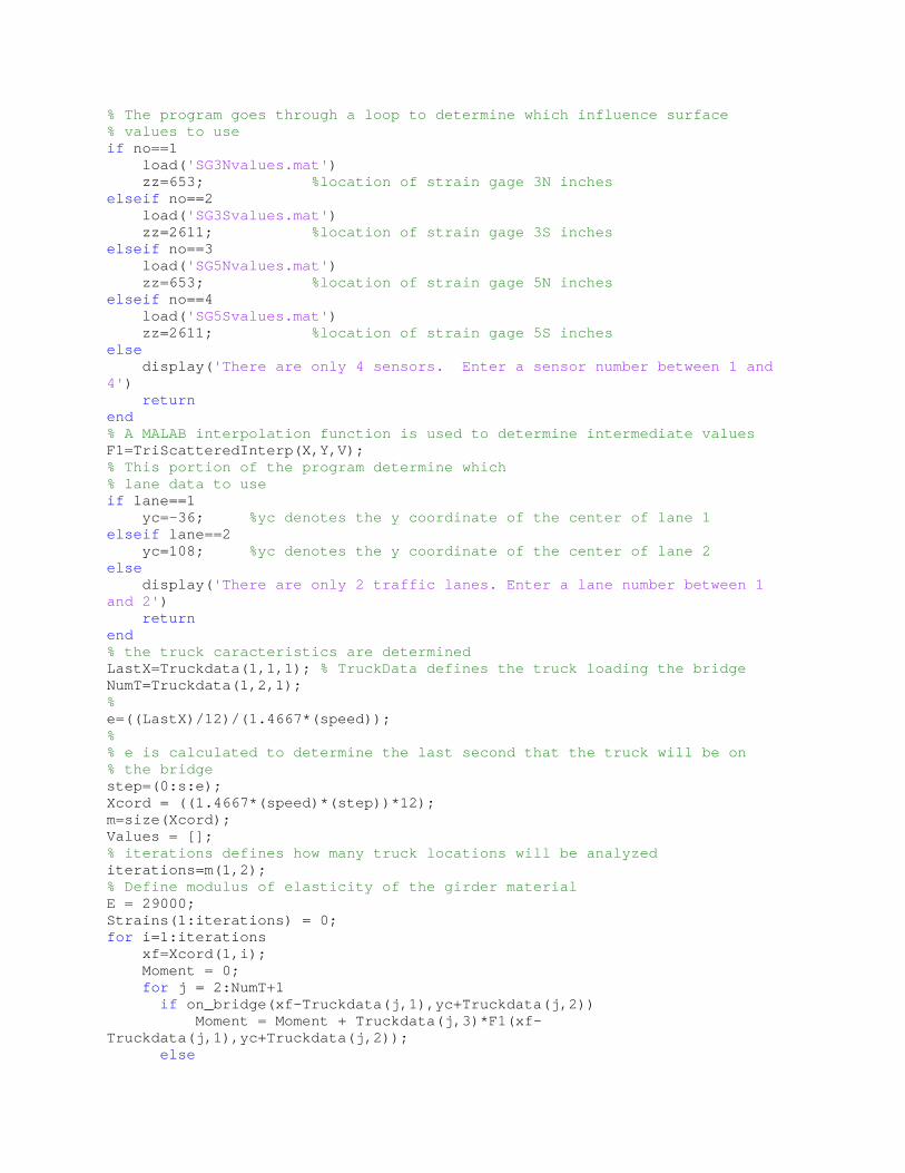
% The program goes through a loop to determine which influence surface % values to use if no==1 load('SG3Nvalues.mat') zz=653; %location of strain gage 3N inches elseif no==2 load('SG3Svalues.mat') zz=2611; %location of strain gage 3S inches elseif no==3 load('SG5Nvalues.mat') zz=653; %location of strain gage 5N inches elseif no==4 load('SG5Svalues.mat') zz=2611; %location of strain gage 5S inches else display('There are only 4 sensors. Enter a sensor number between 1 and 4') return end % A MALAB interpolation function is used to determine intermediate values F1=TriScatteredInterp(X,Y,V); % This portion of the program determine which % lane data to use if lane==1 yc=-36; %yc denotes the y coordinate of the center of lane 1 elseif lane==2 yc=108; %yc denotes the y coordinate of the center of lane 2 else display('There are only 2 traffic lanes. Enter a lane number between 1 and 2') return end % the truck caracteristics are determined LastX=Truckdata(1,1,1); % TruckData defines the truck loading the bridge NumT=Truckdata(1,2,1); % e=((LastX)/12)/(1.4667*(speed)); % % e is calculated to determine the last second that the truck will be on % the bridge step=(0:s:e); Xcord = ((1.4667*(speed)*(step))*12); m=size(Xcord); Values = []; % iterations defines how many truck locations will be analyzed iterations=m(1,2); % Define modulus of elasticity of the girder material E = 29000; Strains(1:iterations) = 0; for i=1:iterations xf=Xcord(1,i); Moment = 0; for j = 2:NumT+1 if on_bridge(xf-Truckdata(j,1),yc+Truckdata(j,2)) Moment = Moment + Truckdata(j,3)*F1(xf-Truckdata(j,1),yc+Truckdata(j,2)); else
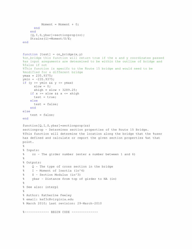
Moment = Moment + 0; end end [Q,I,S,ybar]=sectionprop(zz); Strains(i)=Moment/S/E; end function [test] = on_bridge(x,y) %on_bridge this function will return true if the x and y coordinates passed %as input areguments are determined to be within the outline of bridge and %false if not %This function is specifc to the Route 15 bridge and would need to be %modified for a different bridge ymax = 235.9375; ymin = -235.9375; if (y >= ymin && y <= ymax) xlow = 0; xhigh = xlow + 3289.25; if x >= xlow && x <= xhigh test = true; else test = false; end else test = false; end function[Q,I,S,ybar]=sectionprop(zz) sectionprop - Determines section properties of the Route 15 Bridge. %This function will determine the location along the bridge that the %user has defined and calculate or report the given section properties %at that point. % % Inputs: % zz - The girder number (enter a number between 1 and 6) % % Outputs: % Q - The type of cross section in the bridge % I - Moment of Inertia (in^4) % S - Section Modulus (in^3) % ybar - Distance from top of girder to NA (in) % % See also: interp1 % % Author: Katherine Feeley % email: [email protected] % March 2010; Last revision: 29-March-2010 %------------- BEGIN CODE --------------
if zz<=236 && zz>=0||zz>1028 && zz<=1139.5||zz>2149.751 && zz<=2261.25||zz>3053.25 && zz<=3289.25 Q='PG1'; %Plate Girder 1 - PG1 I=29123.42; S=1040.12; ybar=28; elseif zz>236 && zz<=1028 || zz>2261.25 && zz<=3053.25 Q='PG2'; %Plate Girder 2 - PG2 I=39074.07; S=1126.66; ybar=34.68; elseif zz>1139.5 && zz<=1211.375 Q='PGVAR1'; %PGVAR1 - Use cubic interpolation xx=[1139.5,1211.375]; II=[29123.42,28835.89]; SS=[1040.12,1034.47]; yybar=[28,27.875]; I=interp1(xx,II,zz,'cubic'); S=interp1(xx,SS,zz,'cubic'); ybar=interp1(xx,yybar,zz,'cubic'); elseif zz>1211.375 && zz<=1315.375 Q='PGVAR2'; %PGVAR2 - Use cubic interpolation xx=[1211.375, 1315.375]; II=[42617.12,66832.33]; SS=[1528.87, 1951.31]; yybar=[27.875, 34.25]; I=interp1(xx,II,zz,'cubic'); S=interp1(xx,SS,zz,'cubic'); ybar=interp1(xx,yybar,zz,'cubic'); elseif zz>1315.375 && zz<=1631.375 Q='PGVAR3'; %PGVAR3 - Use cubic interpolation xx=[1315.375, 1631.375]; II=[87225.5, 152455.5]; SS=[152455.5, 3445.32]; yybar=[34.25, 44.25]; I=interp1(xx,II,zz,'cubic'); S=interp1(xx,SS,zz,'cubic'); ybar=interp1(xx,yybar,zz,'cubic'); elseif zz>1631.375 && zz<=1657.875 Q='PG5'; %Plate Girder 5 - PG5 I=152455.5; S=3445.32; ybar=44.25; elseif zz>1657.875 && zz<=1973.875 Q='PGVAR4'; %PGVAR4 - Use cubic interpolation xx=[1657.875, 1973.875]; II=[152455.5, 87225.5]; SS=[3445.32, 2546.73]; yybar=[44.25, 34.25];
I=interp1(xx,II,zz,'cubic'); S=interp1(xx,SS,zz,'cubic'); ybar=interp1(xx,yybar,zz,'cubic'); elseif zz>1973.875 && zz<=2077.875 Q='PGVAR5'; %PGVAR5 - Use cubic interpolation xx=[1973.875, 2077.875]; II=[66832.33, 42617.12]; SS=[1951.31, 1528.87]; yybar=[34.25, 27.875]; I=interp1(xx,II,zz,'cubic'); S=interp1(xx,SS,zz,'cubic'); ybar=interp1(xx,yybar,zz,'cubic'); elseif zz>2077.875 && zz<=2149.751 Q='PGVAR6'; %PGVAR6 - Use cubic interpolation xx=[2077.875, 2149.751]; II=[29123.42, 28835.89]; SS=[1034.47, 1040.12]; yybar=[27.875, 28]; I=interp1(xx,II,zz,'cubic'); S=interp1(xx,SS,zz,'cubic'); ybar=interp1(xx,yybar,zz,'cubic'); elseif zz<0 || zz>3289.25 disp('error') return end %------------- END OF CODE -------------- function [FV ] = GenerateRandomSU3TruckVector %GenerateRandomSU3Trucks % Summary of this function goes here % This function will generate a feature vector of normalized du/dx values % for sensor SG3N produced by SU3 trucks passing over the bridge % % Random variations of truck dimensions an payload are included % % Speed = 40 mph % Lane = lane 1 % SG3N = [t,x,y] vector for gage SG3N % SG3S = [t,x,y] vector for gage SG3S % SG5N = [t,x,y] vector for gage SG5N % SG5S = [t,x,y] vector for gage SG3N Ltruck = 168; Lbridge = 3289.25; LastX = Lbridge + Ltruck; NumT = 6; Lane = 1; Speed = 40; maxPayload = 25.6; meanPayload = maxPayload/2; meanGauge = 40;
meanSpace12 = 120; meanSpace23 = 168; PayLoad = meanPayload + randn(1)*meanPayload/2; Gauge = meanGauge + rand(1)*6; if PayLoad < 0 PayLoad = 0; elseif PayLoad > maxPayload PayLoad = maxPayload; end GVW = 22.6 + PayLoad; AS1 = meanSpace12 + randn(1)*36; AS2 = meanSpace23 + randn(1)*12; TruckData = [LastX NumT 0; 0 -Gauge (10+6*(GVW-22.6)/maxPayload)/2 0 Gauge (10+6*(GVW-22.6)/maxPayload)/2 AS1 -Gauge (6.2+9.8*(GVW-22.6)/maxPayload)/2 AS1 Gauge (6.2+9.8*(GVW-22.6)/maxPayload)/2 AS2 Gauge (6.2+9.8*(GVW-22.6)/maxPayload)/2 AS2 Gauge (6.2+9.8*(GVW-22.6)/maxPayload)/2]; [~,x,y]= route15bridgesimulation7(Lane,1,Speed,TruckData); for i = 2:size(x,2) dudx(i)=((y(i)-y(i-1))/(x(i)-x(i-1))); end; pk = max(dudx); for i = 2:size(x,2) ndudx(i)=((y(i)-y(i-1))/(x(i)-x(i-1)))/pk; end; % 20 values are interpolated at specific locations for i=1:20 idudx(i) = interp1(x,ndudx,650+(i-1)*50); end FV = idudx; end function [FV] = GenerateRandom3S2TruckVector %GenerateRandom3S2TrucksVector % % This function will generate a feature vector of normalized du/dx values % for sensor SG3N produced by 3-S2 truck passing over the bridge % % Speed = 40 mph % Lane = lane 1 % Sensor 1 = SG3N = [t,x,y] vector for gage SG3N % Sensor 2 = SG3S = [t,x,y] vector for gage SG3S % Sensor 3 = SG5N = [t,x,y] vector for gage SG5N % Sensor 4 = SG5S = [t,x,y] vector for gage SG3N Lbridge = 3289.25; NumT = 10; Lane = 1; Speed = 40; Tare = 24; maxPayload = 55; meanPayload = maxPayload/2; meanGauge = 36; meanSpace12 = 120; meanSpace23 = 168; meanSpace34 = 588; meanSpace45 = 636; PayLoad = meanPayload + randn(1)*meanPayload/2; if PayLoad < 0 PayLoad = 0;
elseif PayLoad > maxPayload PayLoad = maxPayload; end Gauge = meanGauge +randn(1)*6; GVW = Tare + PayLoad; AS1 = meanSpace12 + randn(1)*24; AS2 = meanSpace23 + randn(1)*12; AS3 = meanSpace34 + randn(1)*36; AS4 = meanSpace45 + randn(1)*12; if AS4 > meanSpace45 AS3 = AS3 - (meanSpace45 - AS4); end; TruckData = [Lbridge + AS4 NumT 0; 0 -Gauge (10+2*(GVW-Tare)/maxPayload)/2 0 Gauge (10+6*(GVW-Tare)/maxPayload)/2 AS1 -Gauge (5+12*(GVW-Tare)/maxPayload)/2 AS1 Gauge (5+12*(GVW-Tare)/maxPayload)/2 AS2 -Gauge (5+12*(GVW-Tare)/maxPayload)/2 AS2 Gauge (5+12*(GVW-Tare)/maxPayload)/2 AS3 -Gauge (2+15*(GVW-Tare)/maxPayload)/2 AS3 Gauge (2+15*(GVW-Tare)/maxPayload)/2 AS4 -Gauge (2+15*(GVW-Tare)/maxPayload)/2 AS4 Gauge (2+15*(GVW-Tare)/maxPayload)/2]; [~, x, y]= route15bridgesimulation7(Lane,1,Speed,TruckData); for i = 2:size(x,2) dudx(i)=((y(i)-y(i-1))/(x(i)-x(i-1))); end; pk = max(dudx); for i = 2:size(x,2) ndudx(i)=((y(i)-y(i-1))/(x(i)-x(i-1)))/pk; end; for i=1:20 idudx(i) = interp1(x,ndudx,650+(i-1)*50); end FV =idudx; end