For class use only

ACHARYA N.G. RANGA AGRICULTURAL UNIVERSITY

Course No. FDEN-321

Course Title: INSTRUMENTATION & PROCESS CONTROL

Credits: 3 (2 + 1)

Prepared by

Er. B. SREENIVASULA REDDY

Assistant Professor (Food Engineering)

College of Food Science and Technology

Chinnarangapuram, Pulivendula – 516390

YSR (KADAPA) District, Andhra Pradesh

DEPARTMENT OF FOOD ENGINEERING

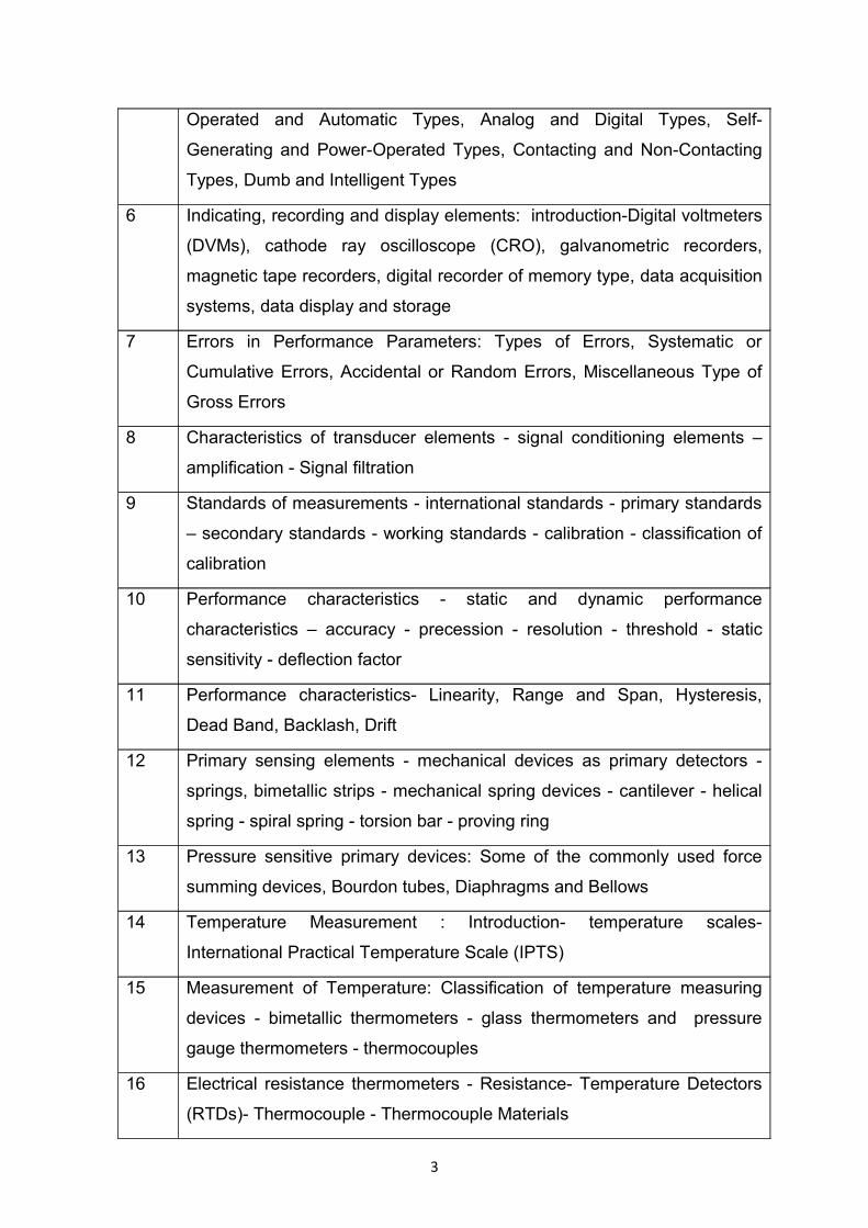
1 Course No : FDEN - 321

2 Title : INSTRUMENTATION & PROCESS CONTROL

3 Credit hours : 3 (2+1)

4 General Objective : To impart knowledge to the students on

instrumentation and process controls used in

food industry

5 Specific Objectives :

a) Theory : By the end of the course the students will be able to

i) understand the different instruments used in different operations of food industries

ii) know about working principles of different instruments used in different operations

b) Practical By the end of the practical exercises the student will be able to

i) identify different instruments and controls used in various operations

ii) identify and tackle the problems encountered in use and operation of different instruments

A) Theory Lecture Outlines

1 Introduction – Instrumentation, Process Control - measurements -

methods of measurements - Direct Methods-In-Direct Methods

2 Primary measurements - secondary measurements - tertiary

measurement -instruments and measurement systems - mechanical

instruments - electrical instruments - electronic instruments

3 Functional elements of measurement systems - basic functional elements

– auxiliary elements - transducer elements - examples of transducer

elements

4 Linear variable differential transformer (LVDT) - advantages of LVDT

- disadvantages of LVDT.

5 Classification of Instruments: Deflection and Null Types, Manually

2

Operated and Automatic Types, Analog and Digital Types, Self-

Generating and Power-Operated Types, Contacting and Non-Contacting

Types, Dumb and Intelligent Types

6 Indicating, recording and display elements: introduction-Digital voltmeters

(DVMs), cathode ray oscilloscope (CRO), galvanometric recorders,

magnetic tape recorders, digital recorder of memory type, data acquisition

systems, data display and storage

7 Errors in Performance Parameters: Types of Errors, Systematic or

Cumulative Errors, Accidental or Random Errors, Miscellaneous Type of

Gross Errors

8 Characteristics of transducer elements - signal conditioning elements –

amplification - Signal filtration

9 Standards of measurements - international standards - primary standards

– secondary standards - working standards - calibration - classification of

calibration

10 Performance characteristics - static and dynamic performance

characteristics – accuracy - precession - resolution - threshold - static

sensitivity - deflection factor

11 Performance characteristics- Linearity, Range and Span, Hysteresis,

Dead Band, Backlash, Drift

12 Primary sensing elements - mechanical devices as primary detectors -

springs, bimetallic strips - mechanical spring devices - cantilever - helical

spring - spiral spring - torsion bar - proving ring

13 Pressure sensitive primary devices: Some of the commonly used force

summing devices, Bourdon tubes, Diaphragms and Bellows

14 Temperature Measurement : Introduction- temperature scales-

International Practical Temperature Scale (IPTS)

15 Measurement of Temperature: Classification of temperature measuring

devices - bimetallic thermometers - glass thermometers and pressure

gauge thermometers - thermocouples

16 Electrical resistance thermometers - Resistance- Temperature Detectors

(RTDs)- Thermocouple - Thermocouple Materials

3

17 Pressure - gauge pressure, absolute pressure, differential pressure,

vacuum - units of pressure - pressure scales - conversion of units- Types

of Pressure Measurement Devices

18 Measurement of pressure : Manometers - U tube manometer - inclined

tube manometer - well type manometer - Properties of Manometric Fluids

19 Elastic Pressure Elements - bourdon tube – bellows - diaphragms

20 Types of Fluid Flow : Steady flow and Unsteady flow- Uniform flow and

Non-uniform flow - One-dimensional flow, two dimensional flow and Three

dimensional flow- Rotational flow and Irrotational flow - Laminar flow and

Turbulent flow.

21 Flow measurement : introduction - primary or quantity meters - positive-

displacement meters - secondary or rate meters - variable head meters 22 The general expression for the rate of flow- Construction of Venturi Meter

23 Construction of Orifice Meter

24 Variable Area Meters- Rotameter; Pitot tube - its advantages - its

limitations

25 Variable Head and Variable Area Flow Meters (Weirs) - Hot Wire

Anemometers - Rotary Vane Meter

26 Measurement of Liquid Level - Direct Liquid Level Measurements - Dip-

stick Method- Sight Glass Method-

27 Hook Gauge- Float Gauge - Float-and-Shaft Liquid Level Gauge

28 Indirect Liquid Level Measurements - Hydrostatic Pressure Level

Measurement Device - Bubbler or Purge Technique for Level

Measurement

29 Capacitance Level Gauge - Ultrasonic Level Gauge - Nucleonic Gauge

30 Control Systems- Introduction- Basic components of the control system-

Classification of Control Systems – Open Loop System - Closed Loop

System - Servo Mechanisms

31 Controllers and Control Action - Pneumatic Controller - Hydraulic

Controllers - Electric Controllers

32 Data Transmission Elements - Electrical Type Data Transmission

Elements - Pneumatic-Type Transmission Elements - Position-Type Data

4

Transmission Elements - Radio-Frequency (RF) Transmission System

B) Practical Class Outlines

1 Study of instrumentation symbols

2 Measurement of temperature by different thermometers

3 Measurement of pressure by U tube manometer (inclined tube manometer)

4 Measurement of liquid level in the tank with the help of Bob and tape

5 Determination of relative humidity by wet and dry bulb thermometer

6 Measurement of velocity of fluid by using venturi meter/orifice meter/pitot tube

7 Measurement of RPM of an electric motor by tachometer

8 Measurement of wind velocity by anemometer

9 Measurement of intensity of sunshine by sunshine recorder

10 Characteristic of valve PI performance, T, P flow and level close leep control

system

11 Measurement of viscosity

12 Calibration of common digital balance

13 Calibration and measurement of OD using spectrophotometer

14 Measurement of running fluid using rotameter

15 Measurement of vacuum - I

16 Measurement of vacuum - II

References

1 B.C. Nakra and K.K.Chaudhary, Instrumentation Measurement and Analysis. Tata

Mc Graw Hill, New Delhi.

2 Sahney and Sahney, A Course in Mechanical Measurement & Instrumentation.

Dhanpat Rai and Sons, New Delhi.

3 K. Krishnaswamy and S. Vijayachitra, Industrial Instrumentation. New Age

International (P) Limited, New Delhi.

5

LECTURE NO.1

INTRODUCTION – INSTRUMENTATION, PROCESS CONTROL - MEASUREMENTS - METHODS OF MEASUREMENTS - DIRECT METHODS-IN-DIRECT METHODS

Instrumentation

Instrumentation is defined as "the art and science of measurement and

control". Instrumentation can be used to refer to the field in which Instrument

technicians and engineers work in, or it can refer to the available methods and

use of instruments.

Instruments are devices which are used to measure attributes of

physical systems. The variable measured can include practically any

measurable variable related to the physical sciences. These variables

commonly include: pressure , flow , temperature , level , density , viscosity ,

radiation , current , voltage , inductance , capacitance , frequency ,chemical

composition , chemical properties , various physical properties, etc.

Instruments can often be viewed in terms of a simple input-output

device. For example, if we "input" some temperature into a thermocouple, it

"outputs" some sort of signal. (Which can later be translated into data.) In the

case of this thermocouple, it will "output" a signal in millivolts.

Process control

The purpose of process control is to reduce the variability in final

products so that legislative requirements and consumers’ expectations of

product quality and safety are met. It also aims to reduce wastage and

production costs by improving the efficiency of processing. Simple control

methods (for example, reading thermometers, noting liquid levels in tanks,

adjusting valves to control the rate of heating or filling), have always been in

place, but they have grown more sophisticated as the scale and complexity of

processing has increased. With increased mechanization, more valves need to

be opened and more motors started or stopped. The timing and sequencing of

these activities has become more critical and any errors by operators has led to

6

more serious quality loss and financial consequences. This has caused a move

away from controls based on the operators’ skill and judgment to technology-

based control systems. Initially, manually operated valves were replaced by

electric or pneumatic operation and switches for motors were relocated onto

control panels. Measurements of process variables, such as levels of liquids in

tanks, pressures, pH, temperatures, etc., were no longer taken at the site of

equipment, but were sent by transmitters to control panels and gradually

processes became more automated.

Automatic control has been developed and applied in almost every

sector of the industry. The impetus for these changes has come from:

• increased competition that forces manufacturers to produce a wider

variety of products more quickly

• escalating labour costs and raw material costs

• increasingly stringent regulations that have resulted from increasing

consumer demands for standardized, safe foods and international

harmonization of legislation and standards.

For some products, new laws require monitoring, reporting and

traceability of all batches produced which has further increased the need for

more sophisticated process control.

All of these requirements have caused manufacturers to upgrade the

effectiveness of their process control and management systems. Advances in

microelectronics and developments in computer software technology, together

with the steady reduction in the cost of computing power, have led to the

development of very fast data processing. This has in turn led to efficient,

sophisticated, interlinked, more operator-friendly and affordable process control

systems being made available to manufacturers. These developments are now

used at all stages in a manufacturing process, including:

• ordering and supplying raw materials

• detailed production planning and supervision

• management of orders, recipes and batches

7

• controlling the flow of product through the process

• controlling process conditions

• evaluation of process and product data (for example, monitoring

temperature profiles during heat processing or chilling

• control of cleaning-in-place procedures

• packaging, warehouse storage and distribution.

MEASUREMENTS

Measurements provide us with a means of describing various

phenomena in quantitative terms. It has been quoted "whatever exists, exists in

some amount". The determination of the amount is measurement all about.

There are innumerable things in nature which have amounts. The

determination of their amounts constitutes the subject of Mechanical

Measurements. The measurements are not necessarily carried out by purely

mechanical means. Quantities like pressure, temperature, displacement, fluid

flow and associated parameters, acoustics and related parameters, and

fundamental quantities like mass, length, and time are typical of those which

are within the scope of mechanical measurements. However, in many

situations, these quantities are not measured by purely mechanical means, but

more often are measured by electrical means by transducing them into an

analogous electrical quantity.

The Measurement of a given quantity is essentially an act or result of

comparison between a quantity whose magnitude (amount) is unknown, with a

similar quantity whose magnitude (amount) is known, the latter quantity being

called a Standard.

Since the two quantities, the amount of which is unknown and another

quantity whose amount is known are compared, the result is expressed in

terms of a numerical value. This is shown in the Fig. 1.1.

8

Fig. 1.1 Fundamental Measuring Process.

In order that the results of measurement are meaningful, the basic

requirements are:

(i) the standard used for comparison purposes must be accurately

defined and should be commonly acceptable,

(ii) the standard must be of the same character as the measurand (the

unknown quantity or the quantity under measurement).

(iii) the apparatus used and the method adopted for the purposes of

comparison must be provable.

METHODS OF MEASUREMENT

The methods of measurement may be broadly classified into two

categories:

Direct Methods.

In-Direct Methods.

Direct Methods.

In these methods, the unknown quantity (also called the measurand) is

directly compared against a standard. The result is expressed as a numerical

number and a unit. Direct methods are quite common for the measurement of

physical quantities like length, mass and time.

Indirect Methods

Measurements by direct methods are not always possible, feasible and,

practicable. These methods in most of the cases, are inaccurate because they

involve human factors. They are also less sensitive. Hence direct methods are

not preferred and are less commonly used.

In engineering applications Measurement Systems are used. These

measurement systems use indirect methods for measurement purposes.

A measurement system consists of a transducing element which

converts the quantity to be measured into an analogous signal. The analogous

9

signal is then processed by some intermediate means and is then fed to the

end devices which present the results of the measurement.

10

LECTURE NO.2

PRIMARY MEASUREMENTS - SECONDARY MEASUREMENTS –

TERTIARY MEASUREMENT -INSTRUMENTS AND MEASUREMENT

SYSTEMS - MECHANICAL INSTRUMENTS - ELECTRICAL INSTRUMENTS -

ELECTRONIC INSTRUMENTS

PRIMARY, SECONDARY AND TERTIARY MEASUREMENTS

Measurements may be classified as primary, secondary and tertiary

based upon whether direct or indirect methods are used.

Primary Measurements:- A primary measurement is one that can be made by

direct observation without involving any conversion (translation) of the

measured quantity into length.

Example:-

(i) the matching of two lengths, such as when determining the length of

an object with a metre rod,

(ii) the matching of two colors, such as when judging the color of red hot

metals

Secondary Measurements:- A secondary measurement involves only one

translation (conversion) to be done on the quantity under measurement to

convert it into a change of length. The measured quantity may be pressure of a

gas, and therefore, may not be observable. Therefore, a secondary

measurement requires,

(i) an instrument which translates pressure changes into length changes,

and

(ii) a length scale or a standard which is calibrated in length units equivalent

to known changes in pressure.

Therefore, in a pressure gauge, the primary signal (pressure) is

transmitted to a translator and the secondary signal (length) is transmitted to

observer's eye.

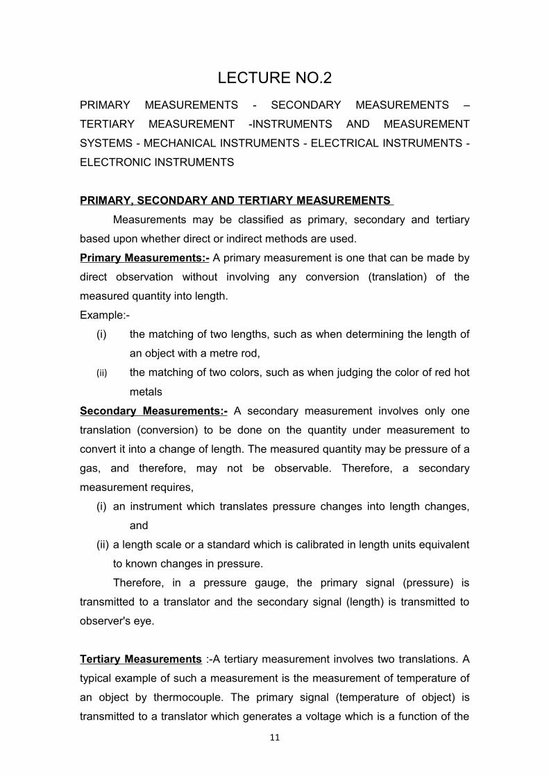
Tertiary Measurements :-A tertiary measurement involves two translations. A

typical example of such a measurement is the measurement of temperature of

an object by thermocouple. The primary signal (temperature of object) is

transmitted to a translator which generates a voltage which is a function of the

11

temperature. Therefore, first translation is temperature to voltage. The voltage,

in turn, is applied to a voltmeter through a pair of wires. The second translation

is then voltage into length. The tertiary signal (length change) is transmitted to

the observer's brain. This tertiary measurement is depicted in, Fig. 2.1.

Fig. 2.1 A typical tertiary measurement.

INSTRUMENTS AND MEASUREMENT SYSTEMS

Measurements involve the use of instruments as a physical means of

determining quantities or variables. The instrument enables the man to

determine the value of unknown quantity or variable. A measuring instrument

exists to provide information about the physical value of some variable being

measured. In simple cases, an instrument consists of a single unit which gives

an output reading or signal according to the unknown variable (measurand)

applied to it. In more complex measurement situations, a measuring instrument

may consist of several separate elements. These elements may consist of

transducing elements which convert the measurand to an analogous form.

The analogous signal is then processed by some intermediate means and then

fed to the end devices to present the results of the measurement for the

purposes of display, record and control. Because of this modular nature of the

elements within it, it is common to refer the measuring instrument as a

measurement system.

MECHANICAL, ELECTRICAL AND ELECTRONIC INSTRUMENTS

The history of development of instruments encompasses three phases

of instruments, viz. : (i) mechanical instruments, (it) electrical instruments and

(iii) electronic instruments.

The three essential elements in modern instruments are :

(i) a detector,

12

(ii) an intermediate transfer device, and

(iii) an indicator, recorder or a storage device.

Mechanical Instruments. These instruments are very reliable for static and

stable conditions. Major disadvantage is unable to respond rapidly to

measurements of dynamic and transient conditions. This is due to the fact that

these instruments have moving parts that are rigid, heavy and bulky and

consequently have a large mass. Mass presents inertia problems and hence

these instruments cannot follow the rapid changes which are involved in

dynamic measurements. Thus it would be virtually impossible to measure a 50

Hz voltage by using a mechanical instrument but it is relatively easy to measure

a slowly varying pressure using these instruments. Another disadvantage of

mechanical instruments is that most of them are a potential source of noise and

cause noise pollution.

Electrical Instruments. Electrical methods of indicating the output of detectors

are more rapid than mechanical methods. Electrical system normally depends

upon a mechanical meter movement as indicating device. This mechanical

movement has some inertia and therefore these instruments have a limited

time (and hence, frequency) response. For example, some electrical recorders

can give full scale response in 0.2 s, the majority of industrial recorders have

responses of 0.5 to 24 s.

Electronic Instruments.: The necessity to step up response time and also the

detection of dynamic changes in certain parameters, which require the

monitoring time of the order of ms and many a times, sµ , have led to the

design of today's electronic instruments and their associated circuitry. These

instruments require use of semiconductor devices. Since in electronic

devices, the only movement involved is that of electrons, the response

time is extremely small on account of very small inertia of electrons. For

example, a Cathode Ray Oscilloscope (CRO) is capable of following dynamic

and transient changes of the order of a few ns (10-9 s).

Another advantage of using electronic devices is that very weak signals

can be detected by using pre-amplifiers and amplifiers. The foremost

importance of the electronic instruments is the power amplification provided by

the electronic amplifiers, which results in higher sensitivity. This is particularly

important in the area of Bio-instrumentation since Bio-electric potentials are

13

very weak i.e., lower than 1 mV. Therefore, these signals are too small to

operate electro-mechanical devices like recorders and they must be amplified.

Additional power may be fed into the system to provide an increased power

output beyond that of the input. Another advantage of electronic instruments is

the ability to obtain indication at a remote location which helps in monitoring

inaccessible or hazardous locations. The most important use of electronic

instrument is their usage in measurement of non-electrical quantities,

where the non-electrical quantity is converted into electrical form through the

use of transducers.

Electronic instruments are light, compact, have a high degree of reliability and

their power consumption is very low.

Communications is a field which is entirely dependent upon the

electronic instruments and associated apparatus. Space communications,

especially, makes use of air borne transmitters and receivers and job of

interpreting the signals is left entirely to the electronic instruments.

In general electronic instruments have (i) a higher sensitivity (ii) a faster

response, (iii) a greater flexibility, (iv) lower weight, (v) lower power

consumption and (vi) a higher degree of reliability

14

LECTURE NO.3

FUNCTIONAL ELEMENTS OF MEASUREMENT SYSTEMS - BASIC

FUNCTIONAL ELEMENTS – AUXILIARY ELEMENTS - TRANSDUCER

ELEMENTS - EXAMPLES OF TRANSDUCER ELEMENTS

FUNCTIONAL ELEMENTS OF MEASUREMENT SYSTEMS

A generalized 'Measurement System' consists of the following:

1. Basic Functional Elements, and

2. Auxiliary Functional Elements.

Basic Functional Elements are those that form the integral parts of all

instruments. They are the following:

1. Transducer Element that senses and converts the desired input to a more

convenient and practicable form to be handled by the measurement system.

2. Signal Conditioning or Intermediate Modifying Element for manipulating /

processing the output of the transducer in a suitable form.

3. Data Presentation Element for giving the information about the measurand

or measured variable in the quantitative form.

Auxiliary Functional Elements are those which may be incorporated in a

particular system depending on the type of requirement, the nature of

measurement technique, etc. They are:

1. Calibration Element to provide a built-in calibration facility.

2. External Power Element to facilitate the working of one or more of the

elements like the transducer element, the signal conditioning element, the

data processing element or the feedback element.

3. Feedback Element to control the variation of the physical quantity that is

being measured. In addition, feedback element is provided in the null-

seeking potentiometric or Wheatstone bridge devices to make them

automatic or self-balancing.

4. Microprocessor Element to facilitate the manipulation of data for the purpose

of simplifying or accelerating the data interpretation. It is always used in

15

conjunction with analog-to-digital converter which is incorporated in the

signal conditioning element.

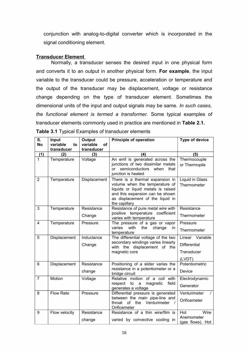
Transducer Element Normally, a transducer senses the desired input in one physical form

and converts it to an output in another physical form. For example, the input

variable to the transducer could be pressure, acceleration or temperature and

the output of the transducer may be displacement, voltage or resistance

change depending on the type of transducer element. Sometimes the

dimensional units of the input and output signals may be same. In such cases,

the functional element is termed a transformer. Some typical examples of

transducer elements commonly used in practice are mentioned in Table 2.1.

Table 3.1 Typical Examples of transducer elements

S.No

Input variable to transducer

Output variable of transducer

Principle of operation Type of device

(1) (2) (3) (4) (5)1 Temperature Voltage An emf is generated across the

junctions of two dissimilar metals or semiconductors when that junction is heated

Thermocouple or Thermopile

2 Temperature Displacement There is a thermal expansion in volume when the temperature of liquids or liquid metals is raised and this expansion can be shown as displacement of the liquid in the capillary

Liquid in Glass Thermometer

3 Temperature Resistance

Change

Resistance of pure metal wire with positive temperature coefficient varies with temperature

Resistance

Thermometer

4 Temperature Pressure The pressure of a gas or vapor varies with the change in temperature

Pressure

Thermometer

5 Displacement Inductance

Change

The differential voltage of the two secondary windings varies linearly with the displacement of the magnetic core

Linear Variable

Differential

Transducer

(LVDT) 6 Displacement Resistance

change

Positioning of a slider varies the resistance in a potentiometer or a bridge circuit

Potentiometric

Device

7 Motion Voltage Relative motion of a coil with respect to a magnetic field generates a voltage

Electrodynamic

Generator

8 Flow Rate Pressure Differential pressure is generated between the main pipe-line and throat of the Venturimeter / Orificemeter

Venturimeter /

Orificemeter

9 Flow velocity Resistance

change

Resistance of a thin wire/film is

varied by convective cooling in

Hot Wire Anemometer (gas flows). Hot

16

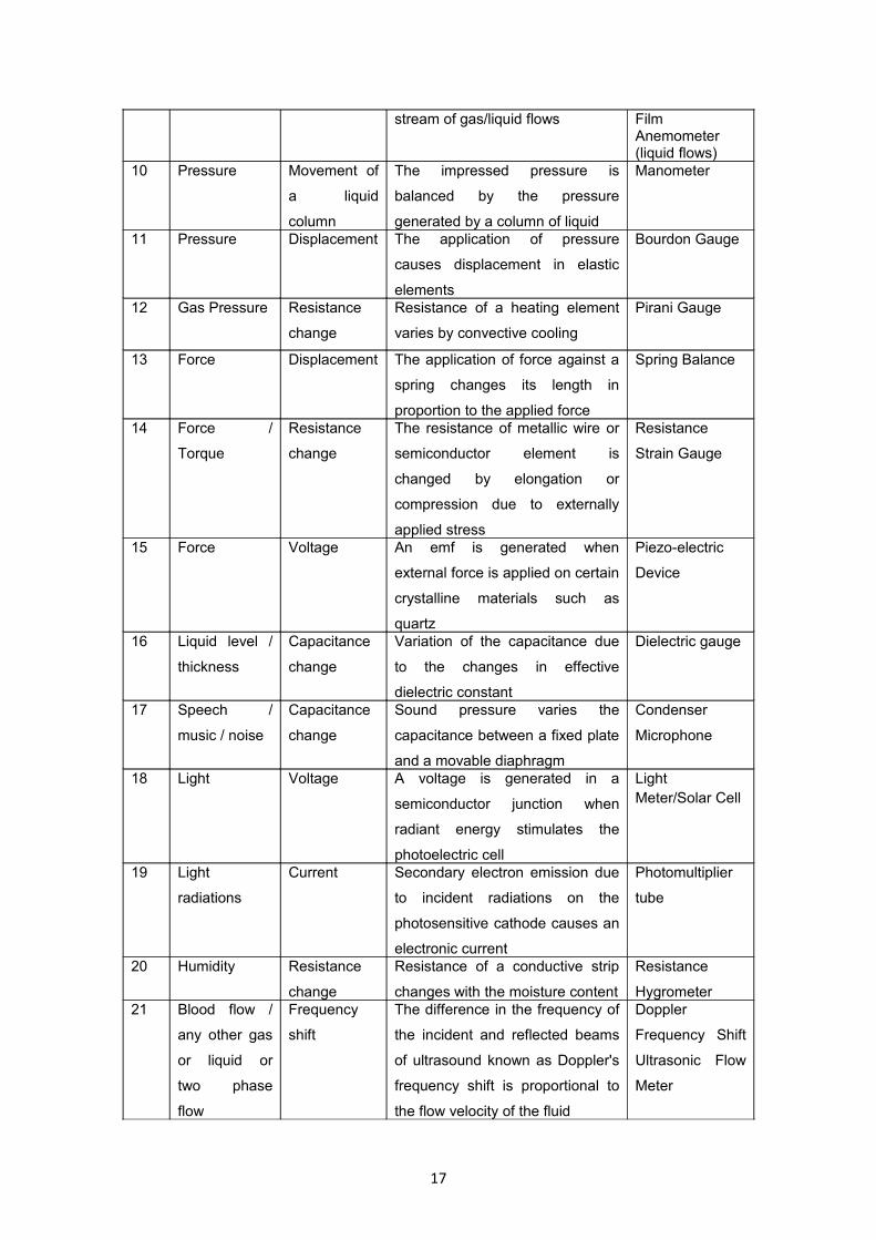
stream of gas/liquid flows Film Anemometer (liquid flows)

10 Pressure Movement of

a liquid

column

The impressed pressure is

balanced by the pressure

generated by a column of liquid

Manometer

11 Pressure Displacement The application of pressure

causes displacement in elastic

elements

Bourdon Gauge

12 Gas Pressure Resistance

change

Resistance of a heating element

varies by convective cooling

Pirani Gauge

13 Force Displacement The application of force against a

spring changes its length in

proportion to the applied force

Spring Balance

14 Force /

Torque

Resistance

change

The resistance of metallic wire or

semiconductor element is

changed by elongation or

compression due to externally

applied stress

Resistance

Strain Gauge

15 Force Voltage An emf is generated when

external force is applied on certain

crystalline materials such as

quartz

Piezo-electric

Device

16 Liquid level /

thickness

Capacitance

change

Variation of the capacitance due

to the changes in effective

dielectric constant

Dielectric gauge

17 Speech /

music / noise

Capacitance

change

Sound pressure varies the

capacitance between a fixed plate

and a movable diaphragm

Condenser

Microphone

18 Light Voltage A voltage is generated in a

semiconductor junction when

radiant energy stimulates the

photoelectric cell

Light Meter/Solar Cell

19 Light

radiations

Current Secondary electron emission due

to incident radiations on the

photosensitive cathode causes an

electronic current

Photomultiplier

tube

20 Humidity Resistance

change

Resistance of a conductive strip

changes with the moisture content

Resistance

Hygrometer21 Blood flow /

any other gas

or liquid or

two phase

flow

Frequency

shift

The difference in the frequency of

the incident and reflected beams

of ultrasound known as Doppler's

frequency shift is proportional to

the flow velocity of the fluid

Doppler

Frequency Shift

Ultrasonic Flow

Meter

17

18

LECTURE NO.4

LINEAR VARIABLE DIFFERENTIAL TRANSFORMER (LVDT) -

ADVANTAGES OF LVDT - DISADVANTAGES OF LVDT.

The most widely used inductive transducer to translate the linear motion

into electrical signals is the linear variable differential Transformer (LVDT). The

basic construction of LVDt is shown in Fig. 4.1. The transformer consists of a

single primary winding P and two secondary windings S1 and S2 wound on a

cylindrical former. The secondary windings have equal number of turns and are

identically placed on either side of the primary winding. The primary winding is

connected to an alternating current source. A movable soft iron core is placed

inside the former. The displacement to be measured is

Fig. 4.1 Linear variable differential Transformer (LVDT)

applied to the arm attached to the soft iron core. In practice the core is made of

high permeability, nickel iron which is hydrogen annealed. This gives low

harmonics, low null voltage and a high sensitivity. This is slotted longitudinally

to reduce eddy current losses. The assembly is placed in stainless steel

housing and the end lids provide electrostatic and electromagnetic shielding.

The frequency of a.c. applied to primary windings may be between 50 Hz to 20

kHz.

Since the primary winding is excited by an alternating current source, it

produces an alternating magnetic field which in turn induces alternating current

voltages in the two secondary windings.

19

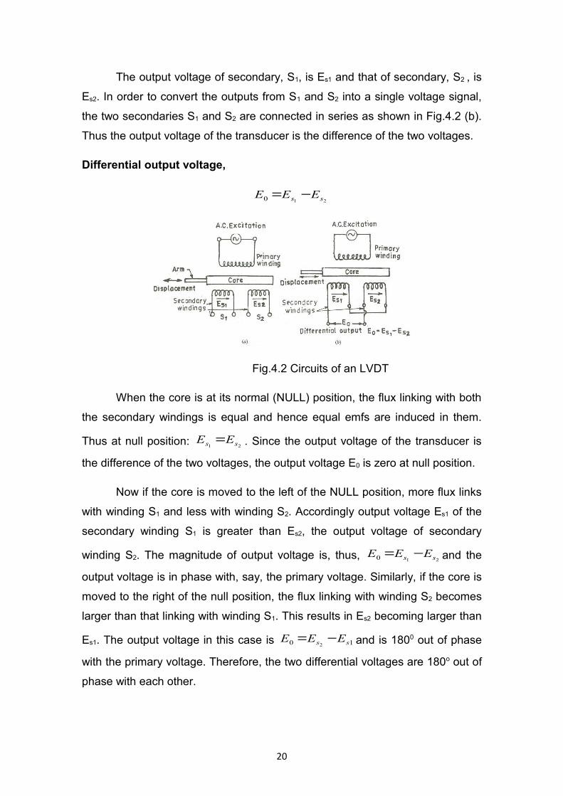
The output voltage of secondary, S1, is Es1 and that of secondary, S2 , is

Es2. In order to convert the outputs from S1 and S2 into a single voltage signal,

the two secondaries S1 and S2 are connected in series as shown in Fig.4.2 (b).

Thus the output voltage of the transducer is the difference of the two voltages.

Differential output voltage,

210 ss EEE −=

Fig.4.2 Circuits of an LVDT

When the core is at its normal (NULL) position, the flux linking with both

the secondary windings is equal and hence equal emfs are induced in them.

Thus at null position: 21 ss EE = . Since the output voltage of the transducer is

the difference of the two voltages, the output voltage E0 is zero at null position.

Now if the core is moved to the left of the NULL position, more flux links

with winding S1 and less with winding S2. Accordingly output voltage Es1 of the

secondary winding S1 is greater than Es2, the output voltage of secondary

winding S2. The magnitude of output voltage is, thus, 210 ss EEE −= and the

output voltage is in phase with, say, the primary voltage. Similarly, if the core is

moved to the right of the null position, the flux linking with winding S2 becomes

larger than that linking with winding S1. This results in Es2 becoming larger than

Es1. The output voltage in this case is 10 2 ss EEE −= and is 1800 out of phase

with the primary voltage. Therefore, the two differential voltages are 180o out of

phase with each other.

20

The amount of voltage change in either secondary winding is

proportional to the amount of movement of the core. Hence, we have an

indication of amount of linear motion.

Advantages of L VDT

1. High range for measurement of displacement. This can be used for

measurement of displacements ranging from 1.25 mm to 250 mm. With

a 0.25 % full scale linearity, it allows measurements down to 0.003 mm.

2. Friction and Electrical Isolation. There is no physical contact between the

movable core and coil structure which means that the LVDT is a

frictionless device.

3. Immunity from External Effects. The separation between LVDT core and

LVDT coils permits the isolation of media such as pressurized, corrosive, or

caustic fluids from the coil assembly by a non-magnetic barrier interposed

between the core and inside of the coil.

4. High input and high sensitivity. The LVDT gives a high output and many a

time there is no need for amplification. The transducer possesses a high

sensitivity which is typically about 40 V/mm.

5. Ruggedness.

6. Low Hysteresis and hence repeatability is excellent under all conditions.

7. Low Power Consumption (less than 1 W).

Disadvantages of LVDTs.

1. Relatively large displacements are required for appreciable differential

output.

2. They are sensitive, to stray magnetic fields but shielding is possible.

This is done by providing magnetic shields with longitudinal slots.

3. Many a time, the transducer performance is affected by vibrations.

4. The receiving instrument must be selected to operate on a.c. signals

or a demodulator network must used if a d.c. output is required.

21

5. The dynamic response is limited mechanically by the mass of the core

6. Temperature affects the performance of the transducer.

22

LECTURE NO.5

CLASSIFICATION OF INSTRUMENTS: DEFLECTION AND NULL TYPES,

MANUALLY OPERATED AND AUTOMATIC TYPES, ANALOG AND DIGITAL

TYPES, SELF-GENERATING AND POWER-OPERATED TYPES,

CONTACTING AND NON-CONTACTING TYPES, DUMB AND INTELLIGENT

TYPES

CLASSIFICATION OF INSTRUMENTS

Instruments may be classified according to their application, mode of

operation, manner of energy conversion, nature of output signal and so on. The

instruments commonly used in practice may be broadly categorized as follows:

Deflection and Null Types

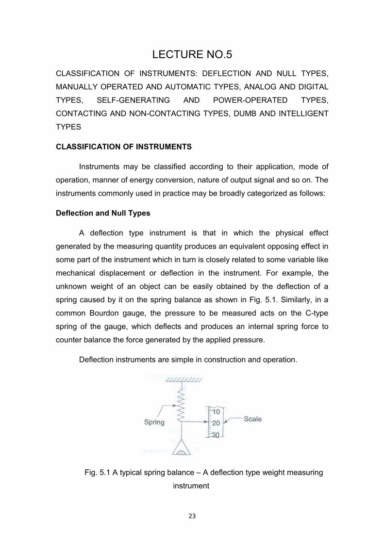
A deflection type instrument is that in which the physical effect

generated by the measuring quantity produces an equivalent opposing effect in

some part of the instrument which in turn is closely related to some variable like

mechanical displacement or deflection in the instrument. For example, the

unknown weight of an object can be easily obtained by the deflection of a

spring caused by it on the spring balance as shown in Fig. 5.1. Similarly, in a

common Bourdon gauge, the pressure to be measured acts on the C-type

spring of the gauge, which deflects and produces an internal spring force to

counter balance the force generated by the applied pressure.

Deflection instruments are simple in construction and operation.

Fig. 5.1 A typical spring balance – A deflection type weight measuring

instrument

23

A null type instrument is the one that is provided with either a manually

operated or automatic balancing device that generates an equivalent opposing

effect to nullify the physical effect caused by the quantity to be measured. The

equivalent null-causing effect in turn provides the measure of the quantity.

Consider a simple situation of measuring the mass of an object by means of an

equal-arm beam balance. An unknown mass, when placed in the pan, causes

the beam and pointer to deflect. Masses of known values are placed on the

other pan till a balanced or null condition is obtained by means of the pointer.

The main advantage of the null-type devices is that they do not interfere with

the state of the measured quantity and thus measurements of such instruments

are extremely accurate.

Manually Operated and Automatic Types

Any instrument which requires the services of human operator is a

manual type of instrument. The instrument becomes automatic if the manual

operation is replaced by an auxiliary device incorporated in the instrument. An

automatic instrument is usually preferred because the dynamic response of

such an instrument is fast and also its operational cost is considerably lower

than that of the corresponding manually operated instrument.

Analog and Digital Types

Analog instruments are those that present the physical variables of

interest in the form of continuous or stepless variations with respect to time.

These instruments usually consist of simple functional elements. Therefore, the

majority of present-day instruments are of analog type as they generally cost

less and are easy to maintain and repair.

On the other hand, digital instruments are those in which the physical

variables are represented by digital quantities which are discrete and vary in

steps. Further, each digital number is a fixed sum of equal steps which is

defined by that number. The relationship of the digital outputs with respect to

time gives the information about the magnitude and the nature of the input

data.

Self-Generating and Power-Operated Types

24

In self-generating (or passive) instruments, the energy requirements of

the instruments are met entirely from the input signal.

On the other hand, power-operated (or active) instruments are those that

require some source of auxiliary power such as compressed air, electricity,

hydraulic supply, etc. for their operation.

Contacting and Non-Contacting Types

A contacting type of instrument is one that is kept in the measuring

medium itself. A clinical thermometer is an example of such instruments.

On the other hand, there are instruments that are of non-contacting or

proximity type. These instruments measure the desired input even though they

are not in close contact with the measuring medium. For example, an optical

pyrometer monitors the temperature of, say, a blast furnace, but is kept out of

contact with the blast furnace. Similarly, a variable reluctance tachometer,

which measures the rpm of a rotating body, is also a proximity type of

instrument.

Dumb and Intelligent Types

A dumb or conventional instrument is that in which the input variable is

measured and displayed, but the data is processed by the observer. For

example, a Bourdon pressure gauge is termed as a dumb instrument because

though it can measure and display a car tyre pressure but the observer has to

judge whether the car tyre air inflation pressure is sufficient or not.

Currently, the advent of microprocessors has provided the means of

incorporating Artificial Intelligence (AI) to a very large number of instruments.

Intelligent or smart instruments process the data in conjunction with

microprocessor ( Pµ ) or an on-line digital computer to provide assistance in

noise reduction, automatic calibration, drift correction, gain adjustments, etc. In

addition, they are quite often equipped with diagnostic subroutines with suitable

alarm generation in case of any type of malfunctioning.

An intelligent or smart instrument may include some or all of the

following:

25

1. The output of the transducer in electrical form.

2. The output of the transducer should be in digital form. Otherwise it has

to be converted to the digital form by means of analog-to-digital

converter (A-D converter).

3. Interface with the digital computer.

4. Software routines for noise reduction, error estimation, self-calibration,

gain adjustment, etc.

5. Software routines for the output driver for suitable digital display or to

provide serial ASCII coded output.

26

LECTURE NO.6

INDICATING, RECORDING AND DISPLAY ELEMENTS: INTRODUCTION-

DIGITAL VOLTMETERS (DVMS), CATHODE RAY OSCILLOSCOPE (CRO),

GALVANOMETRIC RECORDERS, MAGNETIC TAPE RECORDERS, DIGITAL

RECORDER OF MEMORY TYPE, DATA ACQUISITION SYSTEMS, DATA

DISPLAY AND STORAGE

INDICATING, RECORDING AND DISPLAY ELEMENTS

Introduction

The final stage in a measurement system comprises an indicating and /

or a recording element, which gives an indication of the input being measured.

These elements may also be of analog or digital type, depending on whether

the indication or recording is in a continuous or discrete manner. Conventional

voltmeters and ammeters are the simplest examples of analog indicating

instruments, working on the principle of rotation of a coil through which a

current passes, the coil being in a magnetic field.

Digital voltmeters (DVMs) are commonly used as these are convenient

for indication and are briefly described here. Cathode ray oscilloscopes

(CROs) have also been widely used for indicating these signals.

Recording instruments may be galvanometric, potentiometric, servo

types or magnetic tape recorder types. In addition to analog recorders, digital

recorders including digital printers, punched cards or tape recording elements

are also available.

In large-scale systems, data loggers incorporating digital computers are

extensively used for data recording. The present day availability of memory

devices has made the problem of data storage simpler than was previously

possible.

DIGITAL VOLTMETERS (DVMS)

Digital voltmeters convert analog signals into digital presentations which

may be as an indicator or may give an electrical digital output signal. DVMs

measure dc voltage signals. However, other variables like ac voltages,

27

resistances, current, etc. may also be measured with appropriate elements

preceding the input of the DVM.

CATHODE RAY OSCILLOSCOPE (CRO)

As an indicating element, a CRO is widely used in practice. It is

essentially a high input impedance voltage measuring device, capable of

indicating voltage signals from the intermediate elements as a function of time.

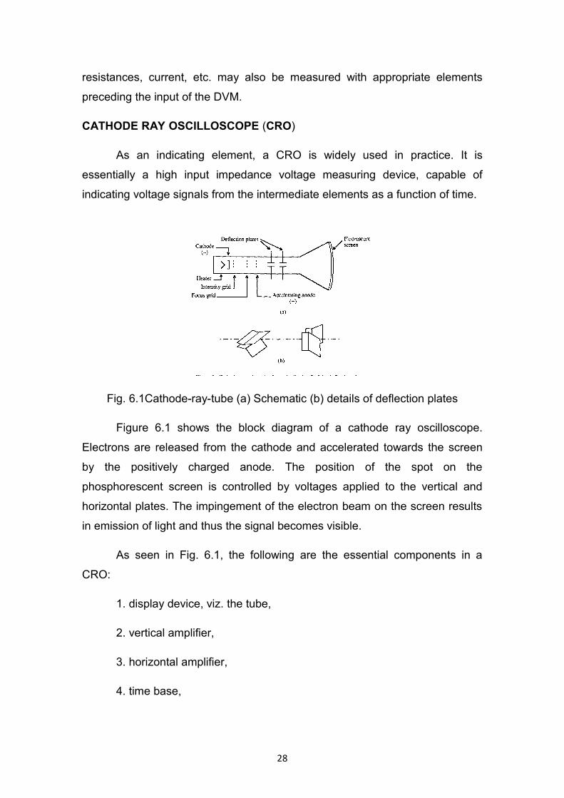
Fig. 6.1Cathode-ray-tube (a) Schematic (b) details of deflection plates

Figure 6.1 shows the block diagram of a cathode ray oscilloscope.

Electrons are released from the cathode and accelerated towards the screen

by the positively charged anode. The position of the spot on the

phosphorescent screen is controlled by voltages applied to the vertical and

horizontal plates. The impingement of the electron beam on the screen results

in emission of light and thus the signal becomes visible.

As seen in Fig. 6.1, the following are the essential components in a

CRO:

1. display device, viz. the tube,

2. vertical amplifier,

3. horizontal amplifier,

4. time base,

28

5. trigger or synchronizing circuit, to start each sweep at a desired time,

for display of signal, and

6. power supplies and internal circuits.

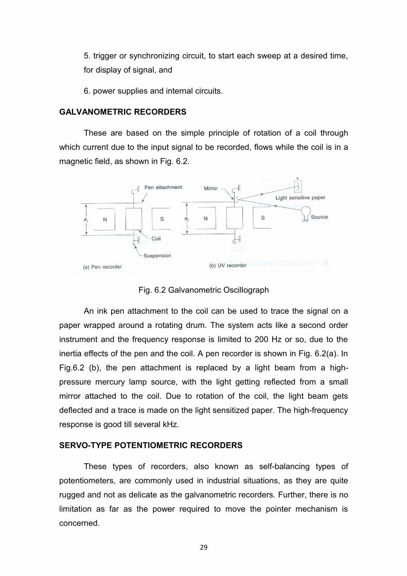
GALVANOMETRIC RECORDERS

These are based on the simple principle of rotation of a coil through

which current due to the input signal to be recorded, flows while the coil is in a

magnetic field, as shown in Fig. 6.2.

Fig. 6.2 Galvanometric Oscillograph

An ink pen attachment to the coil can be used to trace the signal on a

paper wrapped around a rotating drum. The system acts like a second order

instrument and the frequency response is limited to 200 Hz or so, due to the

inertia effects of the pen and the coil. A pen recorder is shown in Fig. 6.2(a). In

Fig.6.2 (b), the pen attachment is replaced by a light beam from a high-

pressure mercury lamp source, with the light getting reflected from a small

mirror attached to the coil. Due to rotation of the coil, the light beam gets

deflected and a trace is made on the light sensitized paper. The high-frequency

response is good till several kHz.

SERVO-TYPE POTENTIOMETRIC RECORDERS

These types of recorders, also known as self-balancing types of

potentiometers, are commonly used in industrial situations, as they are quite

rugged and not as delicate as the galvanometric recorders. Further, there is no

limitation as far as the power required to move the pointer mechanism is

concerned.

29

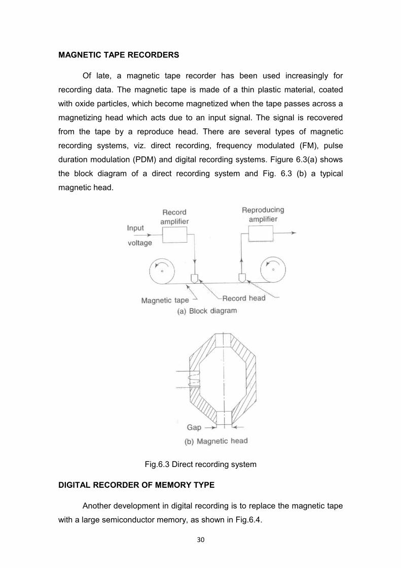
MAGNETIC TAPE RECORDERS

Of late, a magnetic tape recorder has been used increasingly for

recording data. The magnetic tape is made of a thin plastic material, coated

with oxide particles, which become magnetized when the tape passes across a

magnetizing head which acts due to an input signal. The signal is recovered

from the tape by a reproduce head. There are several types of magnetic

recording systems, viz. direct recording, frequency modulated (FM), pulse

duration modulation (PDM) and digital recording systems. Figure 6.3(a) shows

the block diagram of a direct recording system and Fig. 6.3 (b) a typical

magnetic head.

Fig.6.3 Direct recording system

DIGITAL RECORDER OF MEMORY TYPE

Another development in digital recording is to replace the magnetic tape

with a large semiconductor memory, as shown in Fig.6.4.

30

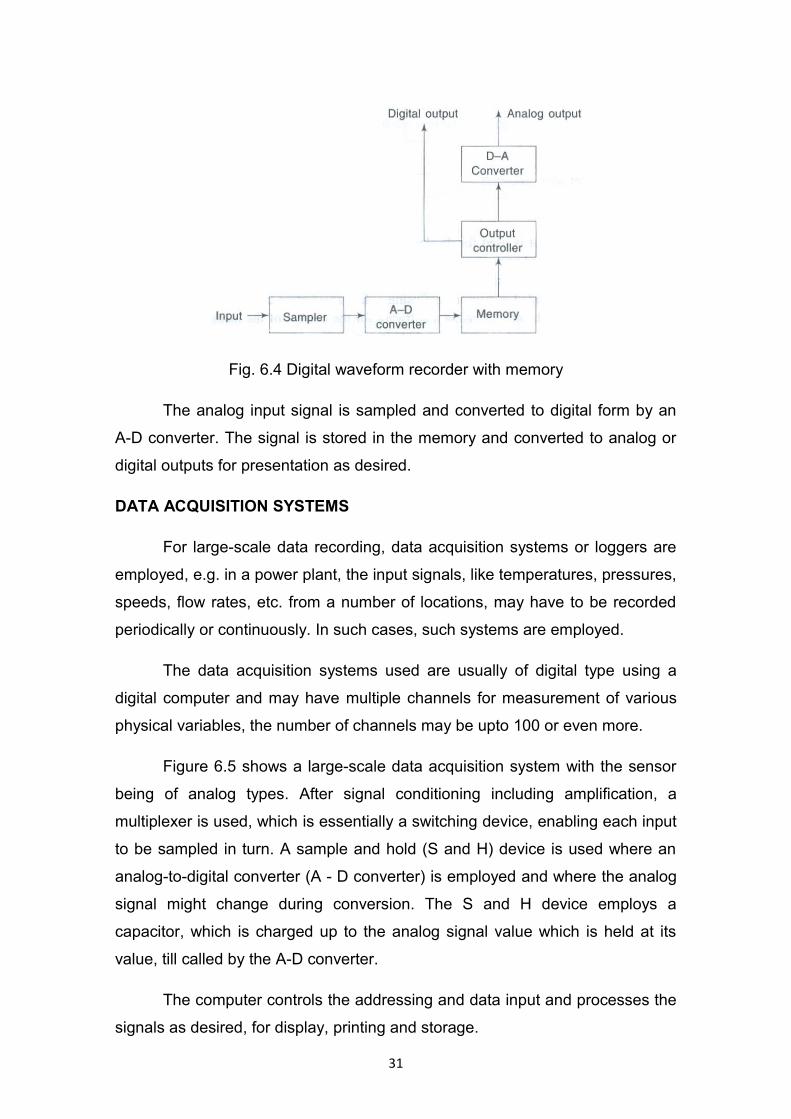
Fig. 6.4 Digital waveform recorder with memory

The analog input signal is sampled and converted to digital form by an

A-D converter. The signal is stored in the memory and converted to analog or

digital outputs for presentation as desired.

DATA ACQUISITION SYSTEMS

For large-scale data recording, data acquisition systems or loggers are

employed, e.g. in a power plant, the input signals, like temperatures, pressures,

speeds, flow rates, etc. from a number of locations, may have to be recorded

periodically or continuously. In such cases, such systems are employed.

The data acquisition systems used are usually of digital type using a

digital computer and may have multiple channels for measurement of various

physical variables, the number of channels may be upto 100 or even more.

Figure 6.5 shows a large-scale data acquisition system with the sensor

being of analog types. After signal conditioning including amplification, a

multiplexer is used, which is essentially a switching device, enabling each input

to be sampled in turn. A sample and hold (S and H) device is used where an

analog-to-digital converter (A - D converter) is employed and where the analog

signal might change during conversion. The S and H device employs a

capacitor, which is charged up to the analog signal value which is held at its

value, till called by the A-D converter.

The computer controls the addressing and data input and processes the

signals as desired, for display, printing and storage.

31

Fig. 6.5 Data acquisition system

The computer monitor unit is used for display, a laser or inkjet or dot

matrix printer for permanent record as per the software used with computer and

the measurement data may be stored in the hard disk and / or floppy disk for

record or communication, where needed.

DATA DISPLAY AND STORAGE

The data may be in analog or digital form as discussed earlier and may

be displayed or stored as such. The display device may be any of the following

types:

1. Analog indicators, comprising motion of a needle on a metre scale.

2. Pen trace or light trace on chart paper recorders.

3. Screen display as in cathode ray oscilloscopes or on large TV screen

display, called visual display unit (VDU).

4. Digital counter of mechanical type, consisting of counter wheel, etc.

5. Digital printer, giving data in printed form.

6. Punches, giving data on punched cards or tapes.

7. Electronic displays, using light emitting diodes (LEDs) or liquid crystal

displays, (LCDs) etc. In LEDs, light is emitted due to the release of

energy as a result of the recombination of unbound free electrons and

holes in the region of the junction. The emission is in the visible region in

case of materials like Gallium Phosphide. LEDs get illuminated ON or

32

OFF, depending on the output being binary 1 or 0. In a microcomputer,

the status of data, address and control buses may be displayed.

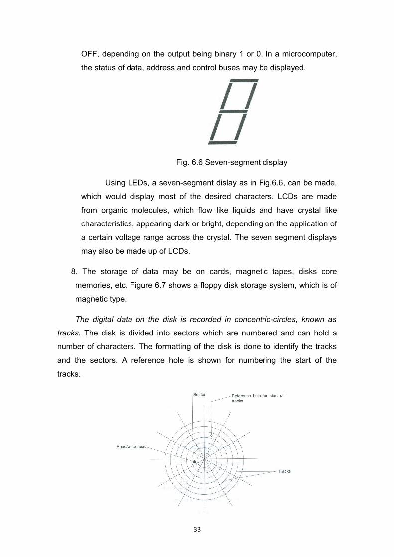
Fig. 6.6 Seven-segment display

Using LEDs, a seven-segment dislay as in Fig.6.6, can be made,

which would display most of the desired characters. LCDs are made

from organic molecules, which flow like liquids and have crystal like

characteristics, appearing dark or bright, depending on the application of

a certain voltage range across the crystal. The seven segment displays

may also be made up of LCDs.

8. The storage of data may be on cards, magnetic tapes, disks core

memories, etc. Figure 6.7 shows a floppy disk storage system, which is of

magnetic type.

The digital data on the disk is recorded in concentric-circles, known as

tracks. The disk is divided into sectors which are numbered and can hold a

number of characters. The formatting of the disk is done to identify the tracks

and the sectors. A reference hole is shown for numbering the start of the

tracks.

33

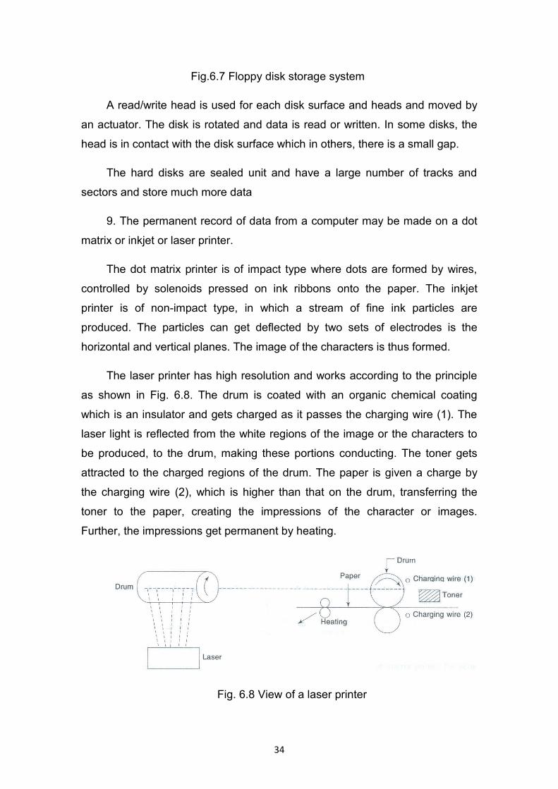
Fig.6.7 Floppy disk storage system

A read/write head is used for each disk surface and heads and moved by

an actuator. The disk is rotated and data is read or written. In some disks, the

head is in contact with the disk surface which in others, there is a small gap.

The hard disks are sealed unit and have a large number of tracks and

sectors and store much more data

9. The permanent record of data from a computer may be made on a dot

matrix or inkjet or laser printer.

The dot matrix printer is of impact type where dots are formed by wires,

controlled by solenoids pressed on ink ribbons onto the paper. The inkjet

printer is of non-impact type, in which a stream of fine ink particles are

produced. The particles can get deflected by two sets of electrodes is the

horizontal and vertical planes. The image of the characters is thus formed.

The laser printer has high resolution and works according to the principle

as shown in Fig. 6.8. The drum is coated with an organic chemical coating

which is an insulator and gets charged as it passes the charging wire (1). The

laser light is reflected from the white regions of the image or the characters to

be produced, to the drum, making these portions conducting. The toner gets

attracted to the charged regions of the drum. The paper is given a charge by

the charging wire (2), which is higher than that on the drum, transferring the

toner to the paper, creating the impressions of the character or images.

Further, the impressions get permanent by heating.

Fig. 6.8 View of a laser printer

34

LECTURE NO.7

ERRORS IN PERFORMANCE PARAMETERS: TYPES OF ERRORS,

SYSTEMATIC OR CUMULATIVE ERRORS, ACCIDENTAL OR RANDOM

ERRORS, MISCELLANEOUS TYPE OF GROSS ERRORS

ERRORS IN PERFORMANCE PARAMETERS

The various static performance parameters of the instruments are

obtained by performing certain specified tests depending on the type of

instrument, the nature of the application, etc. Some salient static performance

parameters are periodically checked by means of a static calibration. This is

accomplished by imposing constant values of 'known' inputs and observing the

resulting outputs.

No measurement can be made with perfect accuracy and precision.

Therefore, it is instructive to know the various types of errors and uncertainties

that are in general, associated with measurement system. Further, it is also

important to know how these errors are propagated.

Types of Errors

Error is defined as the difference between the measured and the true value (as

per standard). The different types of errors can be broadly classified as follows.

Systematic or Cumulative Errors

Such errors are those that tend to have the same magnitude and sign for

a given set of conditions. Because the algebraic sign is the same, they tend to

accumulate and hence are known as cumulative errors. Since such errors alter

the instrument reading by a fixed magnitude and with same sign from one

reading to another, therefore, the error is also commonly termed as instrument

bias. These types of errors are caused due to the following:

Instrument errors:

Certain errors are inherent in the instrument systems. These may be

caused due to poor design / construction of the instrument. Errors in the

divisions of graduated scales, inequality of the balance arms, irregular springs

35

tension, etc., cause such errors. Instrument errors can be avoided by (i)

selecting a suitable instrument for a given application, (ii) applying suitable

correction after determining the amount of instrument error, and (iii) calibrating

the instrument against a suitable standard.

Environmental errors:

These types of errors are caused due to variation of conditions external

to the measuring device, including the conditions in the area surrounding the

instrument. Commonly occurring changes in environmental conditions that may

affect the instrument characteristics are the effects of changes in temperature,

barometric pressure, humidity, wind forces, magnetic or electrostatic fields, etc.

Loading errors

Such errors are caused by the act of measurement on the physical

system being tested. Common examples of this type are: (i) introduction of

additional resistance in the circuit by the measuring milliammeter which may

alter the circuit current by significant amount, (ii) an obstruction type flow meter

may partially block or disturb the flow conditions and consequently the flow rate

shown by the meter may not be same as before the meter installation, and (iii)

introduction of a thermometer alters the thermal capacity of the system and

thereby changes the original state of the system which gives rise to loading

error in the temperature measurement.

Accidental or Random Errors

These errors are caused due to random variations in the parameter or

the system of measurement. Such errors vary in magnitude and may be either

positive or negative on the basis of chance alone. Since these errors are in

either direction, they tend to compensate one another. Therefore, these errors

are also called chance or compensating type of errors. The following are some

of the main contributing factors to random error.

Inconsistencies associated with accurate measurement of small

quantities

36

The outputs of the instruments become inconsistent when very accurate

measurements are being made. This is because when the instruments are built

or adjusted to measure small quantities, the random errors (which are of the

order of the measured quantities) become noticeable.

Presence of certain system defects

System defects such as large dimensional tolerances in mating parts

and the presence of friction contribute to errors that are either positive or

negative depending on the direction of motion. The former causes backlash

error and the latter causes slackness in the meter bearings.

Effect of unrestrained and randomly varying parameters

Chance errors are also caused due to the effect of certain uncontrolled

disturbances which influence the instrument output. Line voltage fluctuations,

vibrations of the instrument supports, etc. are common examples of this type.

Miscellaneous Type of Gross Errors

There are certain other errors that cannot be strictly classified as either

systematic or random as they are partly systematic and partly random.

Therefore, such errors are termed miscellaneous type of gross errors. This

class of errors is mainly caused by the following.

Personal or human errors

These are caused due to the limitations in the human senses. For

example, one may sometimes consistently read the observed value either high

or low and thus introduce systematic errors in the results. While at another time

one may record the observed value slightly differently than the actual reading

and consequently introduce random error in the data.

Errors due to faulty components / adjustments

Sometimes there is a misalignment of moving parts, electrical leakage,

poor optics, etc. in the measuring system.

Improper application of the instrument

37

Errors of this type are caused due to the use of instrument in conditions

which do not conform to the desired design / operating conditions. For

example, extreme vibrations, mechanical shock or pick-up due to electrical

noise could introduce so much gross error as to mask the test information.

38

LECTURE NO.8

CHARACTERISTICS OF TRANSDUCER ELEMENTS - SIGNAL CONDITIONING ELEMENTS – AMPLIFICATION - SIGNAL FILTRATION

Characteristics of transducer element

1. The transducer element should recognize and sense the desired

input signal and should be insensitive to other signals present

simultaneously in the measurand. For example, a velocity transducer

should sense the instantaneous velocity and should be insensitive to the

local pressure or temperature.

2. It should not alter the event to be measured.

3. The output should preferably be electrical to obtain the advantages

of modern computing and display devices.

4. It should have good accuracy.

5. It should have good reproducibility (i.e. precision).

6. It should have amplitude linearity.

7. It should have adequate frequency response (i.e., good dynamic

response).

8. It should not induce phase distortions (i.e. should not induce time lag

between the input and output transducer signals).

9. It should be able to withstand hostile environments without damage

and should maintain the accuracy within acceptable limits.

10. It should have high signal level and low impedance.

11. It should be easily available, reasonably priced and compact in

shape and size (preferably portable).

12. It should have good reliability and ruggedness. In other words, if a

transducer gets dropped by chance, it should still be operative.

13. Leads of the transducer should be sturdy and not be easily pulled

off.

14. The rating of the transducer should be sufficient and it should not break down.

Signal Conditioning Element The output of the transducer element is usually too small to operate an

indicator or a recorder. Therefore, it is suitably processed and modified in the

signal conditioning element so as to obtain the output in the desired form.

39

The transducer signal is fed to the signal conditioning element by

mechanical linkages (levers, gears, etc.), electrical cables, fluid transmission

through liquids or through pneumatic transmission using air. For remote

transmission purposes, special devices like radio links or telemetry systems

may be employed.

The signal conditioning operations that are carried out on the transduced

information may be one or more of the following:

Amplification

Amplification The term amplification means increasing the amplitude of

the signal without affecting its waveform. The reverse phenomenon is termed

attenuation, i.e. reduction of the signal amplitude while retaining its original

waveform. In general, the output of the transducer needs to be amplified in

order to operate an indicator or a recorder. Therefore, a suitable amplifying

element is incorporated in the signal conditioning element which may be one of

the following depending on the type of transducer signal.

1. Mechanical Amplifying

2. Hydraulic/Pneumatic Amplifying

3. Optical Amplifying

4. Electrical Amplifying

1. Mechanical Amplifying Elements such as levers, gears or a combination of

the two, designed to have a multiplying effect on the input transducer signal.

2. Hydraulic/Pneumatic Amplifying Elements employing various types of

valves or constrictions, such as venturimeter / orificemeter, to get significant

variation in pressure with small variation in the input parameters.

3. Optical Amplifying Elements in which lenses, mirrors and combinations of

lenses and mirrors or lamp and scale arrangement are employed to convert the

small input displacement into an output of sizeable magnitude for a convenient

display of the same.

4. Electrical Amplifying Elements employing transistor circuits, integrated

circuits, etc. for boosting the amplitude of the transducer signal. In such

amplifiers we have either of the following:

i

o

V

V

VoltageInput

voltageoutputnAmplicatioVoltage ==

40

i

o

I

I

currentInput

currentoutputnAmplicatioCurrent ==

ii

oo

IV

IV

powerInput

poweroutputgain ==

Signal filtration

The term signal filtration means the removal of unwanted noise signals

that tend to obscure the transducer signal.

The signal filtration element could be any of the following depending on

the type of situation, nature of signal, etc.

1. Mechanical Filters that consist of mechanical elements to protect the

transducer element from various interfering extraneous signals. For example,

the reference junction of a thermocouple is kept in a thermos flask containing

ice. This protects the system from the ambient temperature changes.

2. Pneumatic Filters consisting of a small orifice or venturi to filter out

fluctuations in a pressure signal.

3. Electrical Filters are employed to get rid of stray pick-ups due to electrical

and magnetic fields. They may be simple R-C circuits or any other suitable

electrical filters compatible with the transduced signal.

Other signal conditioning operators Other signal conditioning operators that

can be conveniently employed for electrical signals are

1. Signal Compensation / Signal Linearization.

2. Differentiation / Integration.

3. Analog-to-Digital Conversion.

4. Signal Averaging / Signal Sampling, etc.

41

LECTURE NO.9

STANDARDS OF MEASUREMENTS - INTERNATIONAL STANDARDS - PRIMARY STANDARDS – SECONDARY STANDARDS - WORKING STANDARDS - CALIBRATION - CLASSIFICATION OF CALIBRATION

Standards of Measurements A standard of measurement is defined as the physical representation of

the unit of measurement. A unit of measurement is generally chosen with

reference to an arbitrary material standard or to a natural phenomenon that

includes physical and atomic constants.

For example, the S.I. unit of mass, namely kilogram, was originally

defined as the mass of a cubic decimeter of water at its temperature of

maximum density, i.e. at 4°C. The material representation of this unit is the

International Prototype kilogram which is preserved at the International Bureau

of Weights and Measures at Sevres, France. Further, prior to 1960, the unit of

length was the carefully preserved platinum-iridium bar at Sevres, France. In

1960, this unit was redefined in terms of optical standards, i.e. in terms of the

wavelength of the orange-red light of Kr86 lamp. The standard meter is now

equivalent to 1650763.73 wavelengths of Kr86 orange-red light. Similarly, the

original unit of time was the mean solar second which was defined as 1/86400

of a mean solar day.

Standards of measurements can be classified according to their function

and type of application as:

International standards:

International standards are devices designed and constructed to the

specifications of an international forum. They represent the units of

measurements of various physical quantities to the highest possible accuracy

that is attainable by the use of advanced techniques of production and

measurement technology. These standards are maintained by the International

Bureau of Weights and Measures at Sevres, France.

For example, the International Prototype kilogram, wavelength of Kr86

orange-red lamp and cesium clock are the international standards for mass,

length and time, respectively. However, these standards are not available to an

ordinary user for purposes of day-to-day comparisons and calibrations.

42

Primary standards

Primary standards are devices maintained by standards organizations

/ national laboratories in different parts of the world. These devices represent

the fundamental and derived quantities and are calibrated independently by

absolute measurements. One of the main functions of maintaining primary

standards is to calibrate / check and certify secondary reference standards.

Like international standards, these standards also are not easily available to an

ordinary user of instruments for verification / calibration of working standards.

Secondary standards

Secondary standards are basic reference standards employed by

industrial measurement laboratories. These are maintained by the concerned

laboratory. One of the important functions of an industrial laboratory is the

maintenance and periodic calibration of secondary standards against primary

standards of the national standards laboratory / organization. In addition,

secondary standards are freely available to the ordinary user of instruments for

checking and calibration of working standards.

Working standards

These are high-accuracy devices that are commercially available and

are duly checked and certified against either the primary or secondary

standards. For example, the most widely used industrial working standard of

length are the precision gauge blocks made of steel. These gauge blocks have

two plane parallel surfaces a specified distance apart, with accuracy tolerances

in the 0.25-0.5 micron range. Similarly, a standard cell and a standard resistor

are the working standards of voltage and resistance, respectively. Working

standards are very widely used for calibrating general laboratory instruments,

for carrying out comparison measurements or for checking the quality (range of

accuracy) of industrial products.

Calibration Calibration is the act or result of quantitative comparison between a

known standard and the output of the measuring system. If the output-input

response of the system is linear, then a single-point calibration is sufficient.

However, if the system response is non-linear, then a set of known

standard inputs to the measuring system are employed for calibrating the

corresponding outputs of the system. The process of calibration involves the

43

estimation of uncertainty between the values indicated by the measuring

instrument and the true value of the input.

Calibration procedures can be classified as follows:

Primary calibration

Secondary calibration

Direct calibration with known input source

Indirect calibration

Routine calibration

Primary calibration

When a device/system is calibrated against primary standards, the

procedure is termed primary calibration. After primary calibration, the device

can be employed as a secondary calibration device. The standard resistor

or standard cell available commercially are examples of primary calibration.

Secondary calibration

When a secondary calibration device is used for further calibrating

another device of lesser accuracy, then the procedure is termed secondary

calibration. Secondary calibration devices are very widely used in general

laboratory practice as well as in the industry because they are practical

calibration sources.

Direct calibration with known input source

Direct calibration with a known input source is in general of the same

order of accuracy as primary calibration. Therefore, devices that are calibrated

directly are also used as secondary calibration devices. For example, a turbine

flow meter may be directly calibrated by using the primary measurements

such as weighing a certain amount of water in a tank and recording the time

taken for this quantity of water to flow through the meter. Subsequently, this

flow meter may be used for secondary calibration of other flow metering

devices such as an orificemeter or a venturimeter.

Indirect calibration

Indirect calibration is based on the equivalence of two different devices

that can be employed for measuring a certain physical quantity. This can be

illustrated by a suitable example, say a turbine flow meter. The requirement of

44

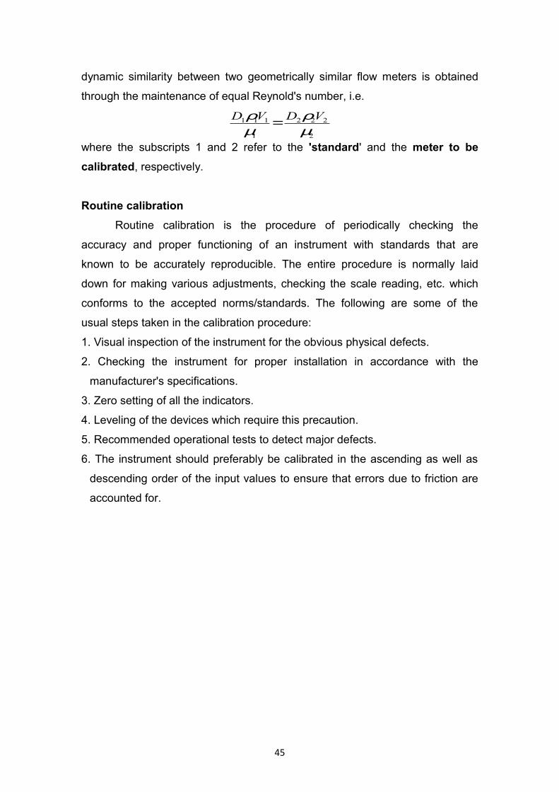
dynamic similarity between two geometrically similar flow meters is obtained

through the maintenance of equal Reynold's number, i.e.

2

222

1

111

µρ

µρ VDVD =

where the subscripts 1 and 2 refer to the 'standard' and the meter to be

calibrated, respectively.

Routine calibration

Routine calibration is the procedure of periodically checking the

accuracy and proper functioning of an instrument with standards that are

known to be accurately reproducible. The entire procedure is normally laid

down for making various adjustments, checking the scale reading, etc. which

conforms to the accepted norms/standards. The following are some of the

usual steps taken in the calibration procedure:

1. Visual inspection of the instrument for the obvious physical defects.

2. Checking the instrument for proper installation in accordance with the

manufacturer's specifications.

3. Zero setting of all the indicators.

4. Leveling of the devices which require this precaution.

5. Recommended operational tests to detect major defects.

6. The instrument should preferably be calibrated in the ascending as well as

descending order of the input values to ensure that errors due to friction are

accounted for.

45

LECTURE NO.10

PERFORMANCE CHARACTERISTICS - STATIC AND DYNAMIC PERFORMANCE CHARACTERISTICS – ACCURACY - PRECESSION - RESOLUTION - THRESHOLD - STATIC SENSITIVITY - DEFLECTION FACTOR

PERFORMANCE CHARACTERISTICS

The measurement system characteristics can be divided into two categories:

(i) Static characteristics and (ii) Dynamic characteristics.

Static characteristics of a measurement system are, in general, those

that must be considered when the system or instrument is used to measure a

condition not varying with time.

However many measurements are concerned with rapidly varying

quantities and, therefore, for such cases the dynamic relations which exist

between the output and the input are examined. This is normally done with the

help of differential equations. Performance criteria based upon dynamic

relations constitute the Dynamic Characteristics.

Static characteristics

Accuracy

Accuracy of a measuring system is defined as the closeness of the

instrument output to the true value of the measured quantity. It is also specified

as the percentage deviation or inaccuracy of the measurement from the true

value. For example, if a chemical balance reads 1 g with an error of 10-2g, the

accuracy of the measurement would be specified as 1%.

Accuracy of the instrument mainly depends on the inherent limitations of

the instrument as well as on the shortcomings in the measurement process. In

fact, these are the major parameters that are responsible for systematic or

cumulative errors. For example, the accuracy of a common laboratory

micrometer depends on instrument errors like zero error, errors in the pitch

of screw, anvil shape, etc. and in the measurement process errors are

caused due to temperature variation effect, applied torque, etc.

46

The accuracy of the instruments can be specified in either of the

following forms:

100 valuetrue

valuetrue- valuemeasured value trueof Percentage 1. ×=

100 valuescale maximum

valuetrue- valuemeasured deflection scale-full of Percentage.2 ×=

Precision

Precision is defined as the ability of the instrument to reproduce a

certain set of readings within a given accuracy. For example, if a particular

transducer is subjected to an accurately known input and if the repeated read

outs of the instrument lie within say ± 1 %, then the precision or alternatively

the precision error of the instrument would be stated as ± 1%. Thus, a highly

precise instrument is one that gives the same output information, for a given

input information when the reading is repeated a large number of times.

Precision of an instrument is in fact, dependent on the repeatability. The

term repeatability can be defined as the ability of the instrument to reproduce a

group of measurements of the same measured quantity, made by the same

observer, using the same instrument, under the same conditions. The precision

of the instrument depends on the factors that cause random or accidental

errors. The extent of random errors of alternatively the precision of a given set

of measurements can be quantified by performing the statistical analysis.

Accuracy v/s Precision

The accuracy represents the degree of correctness of the measured

value with respect to the true value and the precision represents degree of

repeatability of several independent measurements of the desired input at the

same reference conditions.

Accuracy and precision are dependent on the systematic and random

errors, respectively. Therefore, in any experiment both the quantities have to be

evaluated. The former is determined by proper calibration of the

instrument and the latter by statistical analysis. However, it is instructive to

note that a precise measurement may not necessarily be accurate and vice

versa. To illustrate this statement we take the example of a person doing

47

shooting practice on a target. He can hit the target with the following

possibilities as shown in Fig. 10.1.

1. One possibility is that the person hits all the bullets on the target plate

on the outer circle and misses the bull's eye [Fig. 10.1(a)]. This is a

case of high precision but poor accuracy.

2. Second possibility is that the bullets are placed as shown in Fig. 10.1

(b). In this case, the bullet hits are placed symmetrically with respect

to the bull's eye but are not spaced closely. Therefore, this is case of

good average accuracy but poor precision.

3. A third possibility is that all the bullets hit the bull's eye and are also

spaced closely [Fig. 10.1 (c)]. As is clear from the diagram, this is a

case of high accuracy and high precision.

4. Lastly, if the bullets hit the target plate in a random manner as shown

in Fig. 10.1 (d), then this is a case of poor precision as well as poor

accuracy.

Fig.10.1 Illustration of degree of accuracy and precision in a typical target shooting experiment

Based on the above discussion, it may be stated that in any experiment

the accuracy of the observations can be improved but not beyond the precision

of the apparatus.

Resolution (or Discrimination)

It is defined as the smallest increment in the measured value that can be

detected with certainty by the instrument. In other words, it is the degree of

fineness with which a measurement can be made. The least count of any

instrument is taken as the resolution of the instrument. For example, a ruler

with a least count of 1 mm may be used to measure to the nearest 0.5 mm by

48

interpolation. Therefore, its resolution is considered as 0.5 mm. A high

resolution instrument is one that can detect smallest possible variation in the

input.

Threshold

It is a particular case of resolution. It is defined as the minimum value of

input below which no output can be detected. It is instructive to note that

resolution refers to the smallest measurable input above the zero value. Both

threshold and resolution can either be specified as absolute quantities in terms

of input units or as percentage of full scale deflection.

Both threshold and resolution are not zero because of various factors

like friction between moving parts, play or looseness in joints (more correctly

termed as backlash), inertia of the moving parts, length of the scale, spacing of

graduations, size of the pointer, parallax effect, etc.

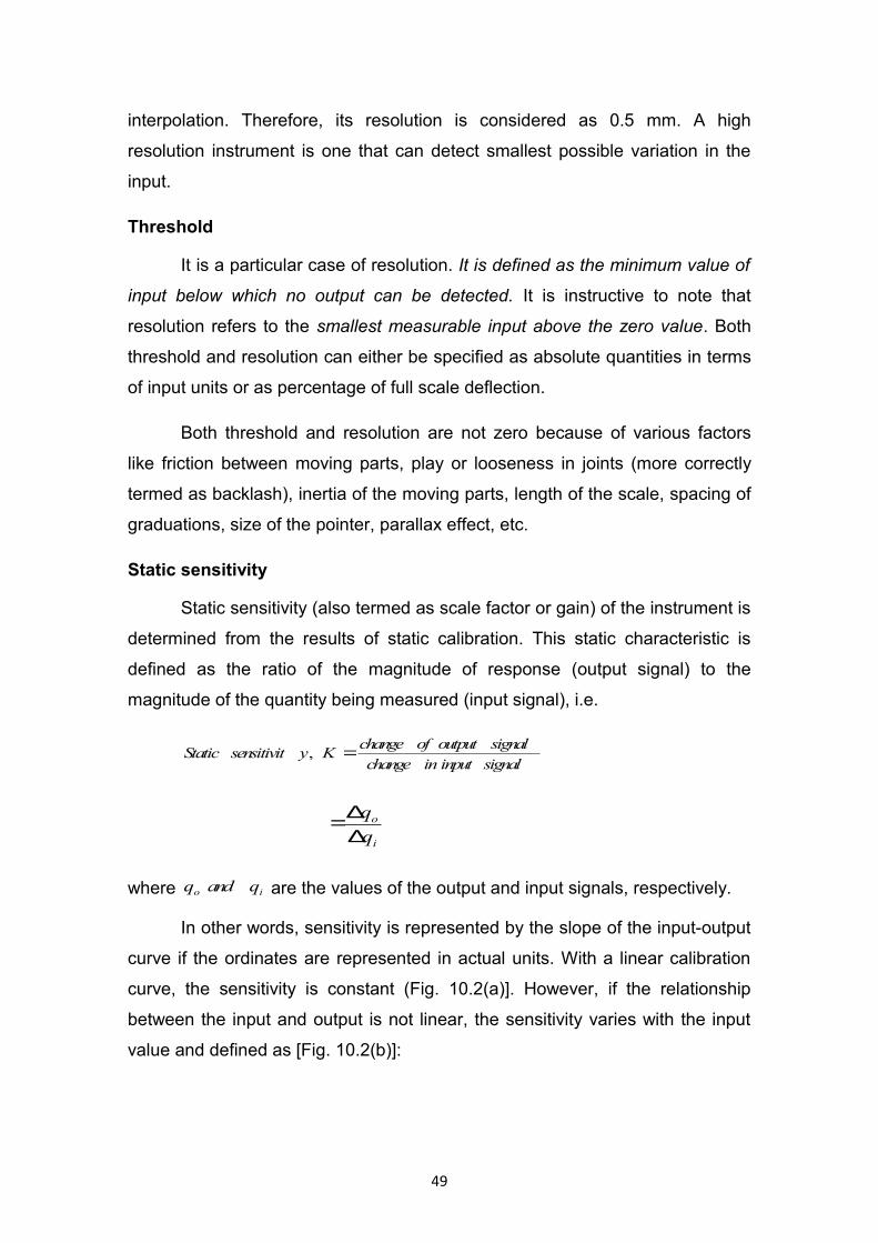
Static sensitivity

Static sensitivity (also termed as scale factor or gain) of the instrument is

determined from the results of static calibration. This static characteristic is

defined as the ratio of the magnitude of response (output signal) to the

magnitude of the quantity being measured (input signal), i.e.

signalinputinchangesignaloutputofchange

KysensitivitStatic =,

i

o

q

q

∆∆=

where io qandq are the values of the output and input signals, respectively.

In other words, sensitivity is represented by the slope of the input-output

curve if the ordinates are represented in actual units. With a linear calibration

curve, the sensitivity is constant (Fig. 10.2(a)]. However, if the relationship

between the input and output is not linear, the sensitivity varies with the input

value and defined as [Fig. 10.2(b)]:

49

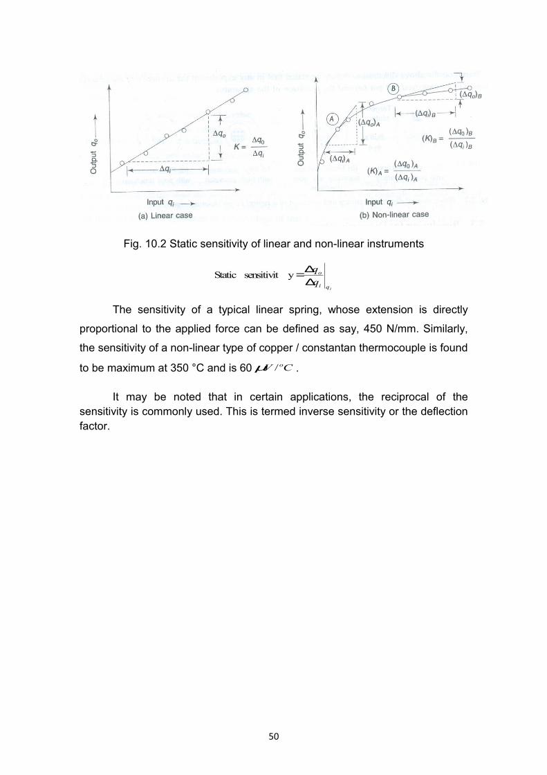
Fig. 10.2 Static sensitivity of linear and non-linear instruments

iqi

o

q

q

∆∆=ysensitivit Static

The sensitivity of a typical linear spring, whose extension is directly

proportional to the applied force can be defined as say, 450 N/mm. Similarly,

the sensitivity of a non-linear type of copper / constantan thermocouple is found

to be maximum at 350 °C and is 60 CV o/µ .

It may be noted that in certain applications, the reciprocal of the sensitivity is commonly used. This is termed inverse sensitivity or the deflection factor.

50

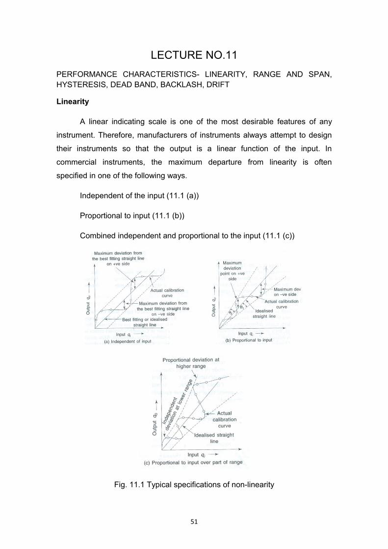
LECTURE NO.11

PERFORMANCE CHARACTERISTICS- LINEARITY, RANGE AND SPAN, HYSTERESIS, DEAD BAND, BACKLASH, DRIFT

Linearity

A linear indicating scale is one of the most desirable features of any

instrument. Therefore, manufacturers of instruments always attempt to design

their instruments so that the output is a linear function of the input. In

commercial instruments, the maximum departure from linearity is often

specified in one of the following ways.

Independent of the input (11.1 (a))

Proportional to input (11.1 (b))

Combined independent and proportional to the input (11.1 (c))

Fig. 11.1 Typical specifications of non-linearity

51

The non-linearity of a complex type of calibration curve is obtained as

say ± y % of full-scale deflection and also as ± x % of the input value. The non-

linearity of the instrument is then stated as ± y % of full scale or ± x % of the

input, whichever is greater.

Range and Span

The range of the instrument is specified by the lower and upper limits in

which it is designed to operate for measuring, indicating or recording the

measured variable. The algebraic difference between the upper and lower

range values is termed as the span of the instrument. The range of the

instrument can either be unidirectional (e.g., 0-100°C) or bidirectional (e.g., -10

to 100°C) or it can be expanded type (e.g., 80 -100°C) or zero suppressed

(e.g., 5 - 40°C).

The over-range (or overload capacity) of the instrument is the maximum

value of measurand that can be applied to the instrument without causing a

perceptible change in its operating characteristics. Further, the recovery time of

the instrument is the amount of time elapsed after the removal of the overload

conditions before it performs again within the specified tolerances.

Hysteresis

It is defined as the magnitude of error caused in the output for a given

value of input, when this value is approached from opposite directions, i.e. from

ascending order and then descending order. This is caused by backlash,

elastic deformations, magnetic characteristics, but is mainly caused due to

frictional effects.

52

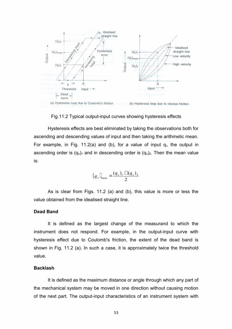
Fig.11.2 Typical output-input curves showing hysteresis effects

Hysteresis effects are best eliminated by taking the observations both for

ascending and descending values of input and then taking the arithmetic mean.

For example, in Fig. 11.2(a) and (b), for a value of input qi, the output in

ascending order is (qo)1 and in descending order is (qo)2. Then the mean value

is:

( )2

)()( 21 oomeano

qqq

+=

As is clear from Figs. 11.2 (a) and (b), this value is more or less the

value obtained from the idealised straight line.

Dead Band

It is defined as the largest change of the measurand to which the

instrument does not respond. For example, in the output-input curve with

hysteresis effect due to Coulomb's friction, the extent of the dead band is

shown in Fig. 11.2 (a). In such a case, it is approximately twice the threshold

value.

Backlash

It is defined as the maximum distance or angle through which any part of

the mechanical system may be moved in one direction without causing motion

of the next part. The output-input characteristics of an instrument system with

53

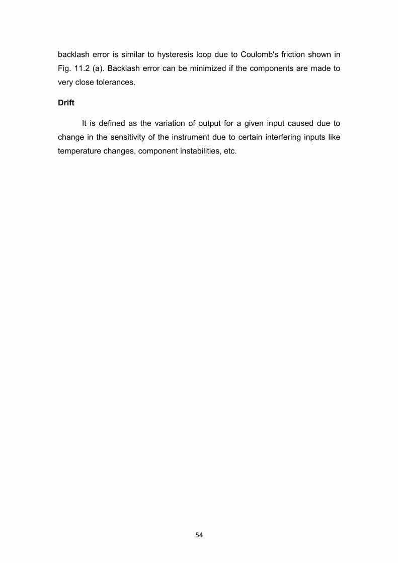
backlash error is similar to hysteresis loop due to Coulomb's friction shown in

Fig. 11.2 (a). Backlash error can be minimized if the components are made to

very close tolerances.

Drift

It is defined as the variation of output for a given input caused due to

change in the sensitivity of the instrument due to certain interfering inputs like

temperature changes, component instabilities, etc.

54

LECTURE NO.12

PRIMARY SENSING ELEMENTS - MECHANICAL DEVICES AS PRIMARY DETECTORS - SPRINGS, BIMETALLIC STRIPS - MECHANICAL SPRING DEVICES - CANTILEVER - HELICAL SPRING - SPIRAL SPRING - TORSION BAR - PROVING RING

PRIMARY SENSING ELEMENTS

Introduction

The measurand in an instrumentation system makes its first contact with

a Primary Detection Element or an Input Device. There are variety of

measurands to be measured. These include process variables like

temperature, pressure and flow rate. The measurands also include electrical

quantities like current, voltage, resistance, inductance, capacitance, frequency,

phase angle, power and magnetic quantities like flux, flux density, reluctance

etc.

All these quantities require a primary detection element and / or a

transducer to be converted into another analogous format which is acceptable

by the later stages of the measurement system.

Mechanical Devices as Primary Detectors

There are a number of mechanical quantities which are to be measured.

Some of these quantities are listed in Table 12.1 along with their modes of

operation for the purposes of measurement.

The initial concept of converting an applied force into a displacement is

basic to many types of primary sensing elements. The mechanical elements

which are used to convert the applied force into displacement are usually

elastic members. There are many types of these elastic members. They can be

classified into three categories as:

i) Direct tension or compression type

ii) Bending type

iii) Torsion type

Table 12.1 Mechanical Quantities and their modes of operation

55

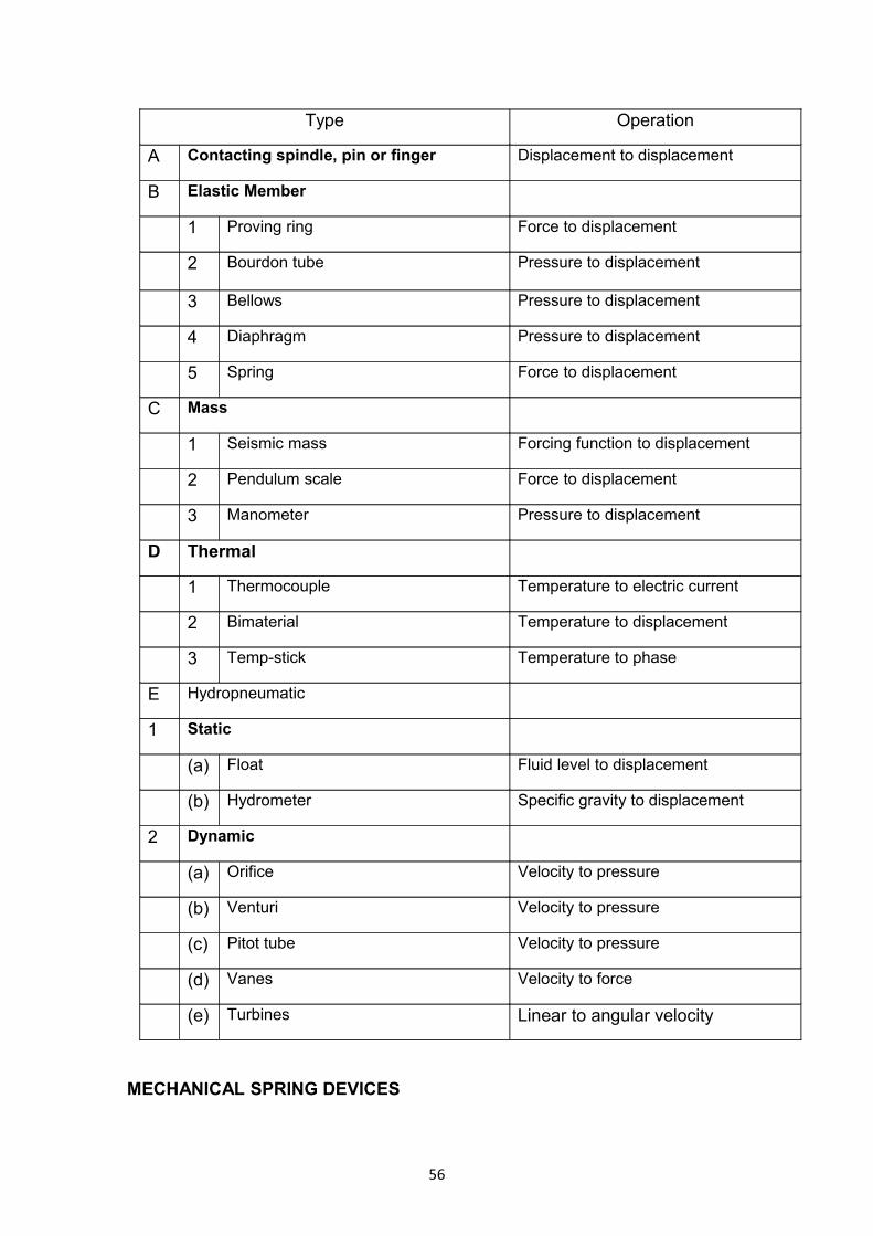
Type Operation

A Contacting spindle, pin or finger Displacement to displacement

B Elastic Member

1 Proving ring Force to displacement

2 Bourdon tube Pressure to displacement

3 Bellows Pressure to displacement

4 Diaphragm Pressure to displacement

5 Spring Force to displacement

C Mass

1 Seismic mass Forcing function to displacement

2 Pendulum scale Force to displacement

3 Manometer Pressure to displacement

D Thermal

1 Thermocouple Temperature to electric current

2 Bimaterial Temperature to displacement

3 Temp-stick Temperature to phase

E Hydropneumatic

1 Static

(a) Float Fluid level to displacement

(b) Hydrometer Specific gravity to displacement

2 Dynamic

(a) Orifice Velocity to pressure

(b) Venturi Velocity to pressure

(c) Pitot tube Velocity to pressure

(d) Vanes Velocity to force

(e) Turbines Linear to angular velocity

MECHANICAL SPRING DEVICES

56

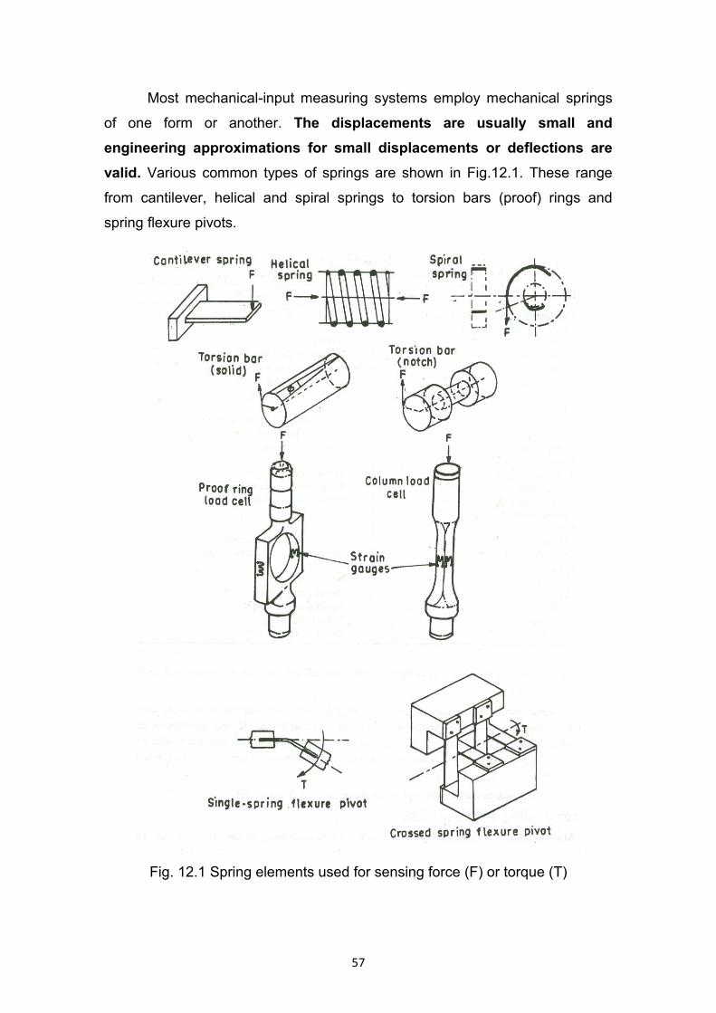
Most mechanical-input measuring systems employ mechanical springs

of one form or another. The displacements are usually small and

engineering approximations for small displacements or deflections are

valid. Various common types of springs are shown in Fig.12.1. These range

from cantilever, helical and spiral springs to torsion bars (proof) rings and

spring flexure pivots.

Fig. 12.1 Spring elements used for sensing force (F) or torque (T)

57

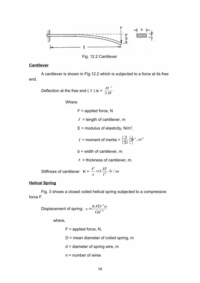
Fig. 12.2 Cantilever

Cantilever

A cantilever is shown in Fig.12.2 which is subjected to a force at its free end.

Deflection at the free end ( x ) is = EI

Fl

3

3

Where

F = applied force, N

l = length of cantilever, m

E = modulus of elasticity, N/m2,

I = moment of inertia = 43 ,12

1mbt

b = width of cantilever, m

t = thickness of cantilever, m.

Stiffness of cantilever K = mNl

EI

x

F/3

3=

Helical Spring

Fig. 3 shows a closed coiled helical spring subjected to a compressive force F.

Displacement of spring: 4

38

Gd

nFDx=

where,

F = applied force, N,

D = mean diameter of coiled spring, m

d = diameter of spring wire, m

n = number of wires

58

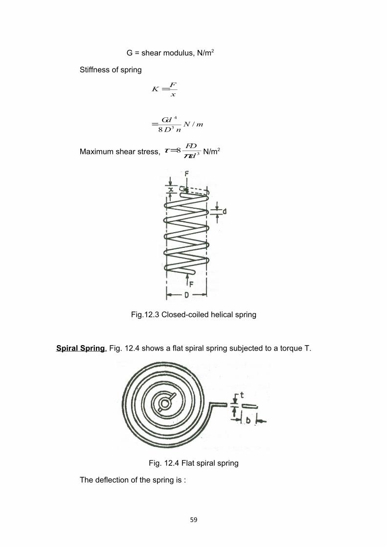
G = shear modulus, N/m2

Stiffness of spring

x

FK=

mNnD

Gd/

8 3

4

=

Maximum shear stress, 38

d

FD

πτ= N/m2

Fig.12.3 Closed-coiled helical spring

Spiral Spring . Fig. 12.4 shows a flat spiral spring subjected to a torque T.

Fig. 12.4 Flat spiral spring

The deflection of the spring is :

59

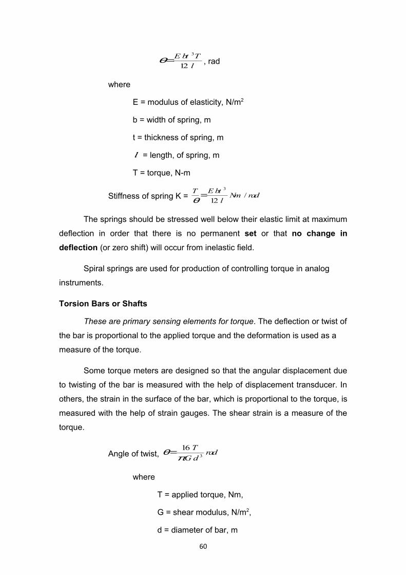
l

TbtE

12

3

=θ , rad

where

E = modulus of elasticity, N/m2

b = width of spring, m

t = thickness of spring, m

l = length, of spring, m

T = torque, N-m

Stiffness of spring K = radNml

btET/

12

3

=θ

The springs should be stressed well below their elastic limit at maximum

deflection in order that there is no permanent set or that no change in

deflection (or zero shift) will occur from inelastic field.

Spiral springs are used for production of controlling torque in analog

instruments.

Torsion Bars or Shafts

These are primary sensing elements for torque. The deflection or twist of

the bar is proportional to the applied torque and the deformation is used as a

measure of the torque.

Some torque meters are designed so that the angular displacement due

to twisting of the bar is measured with the help of displacement transducer. In

others, the strain in the surface of the bar, which is proportional to the torque, is

measured with the help of strain gauges. The shear strain is a measure of the

torque.

Angle of twist, raddG

T3

16

πθ=

where

T = applied torque, Nm,

G = shear modulus, N/m2,

d = diameter of bar, m

60

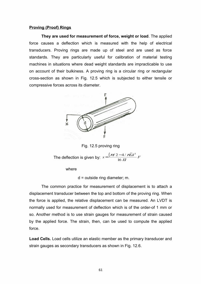
Proving (Proof) Rings

They are used for measurement of force, weight or load. The applied

force causes a deflection which is measured with the help of electrical

transducers. Proving rings are made up of steel and are used as force

standards. They are particularly useful for calibration of material testing

machines in situations where dead weight standards are impracticable to use

on account of their bulkiness. A proving ring is a circular ring or rectangular

cross-section as shown in Fig. 12.5 which is subjected to either tensile or

compressive forces across its diameter.

Fig. 12.5 proving ring

The deflection is given by: ( )

FEI

dx

16

/42/ 3ππ −=

where

d = outside ring diameter; m.

The common practice for measurement of displacement is to attach a

displacement transducer between the top and bottom of the proving ring. When

the force is applied, the relative displacement can be measured. An LVDT is

normally used for measurement of deflection which is of the order-of 1 mm or

so. Another method is to use strain gauges for measurement of strain caused

by the applied force. The strain, then, can be used to compute the applied

force.

Load Cells. Load cells utilize an elastic member as the primary transducer and

strain gauges as secondary transducers as shown in Fig. 12.6.

61

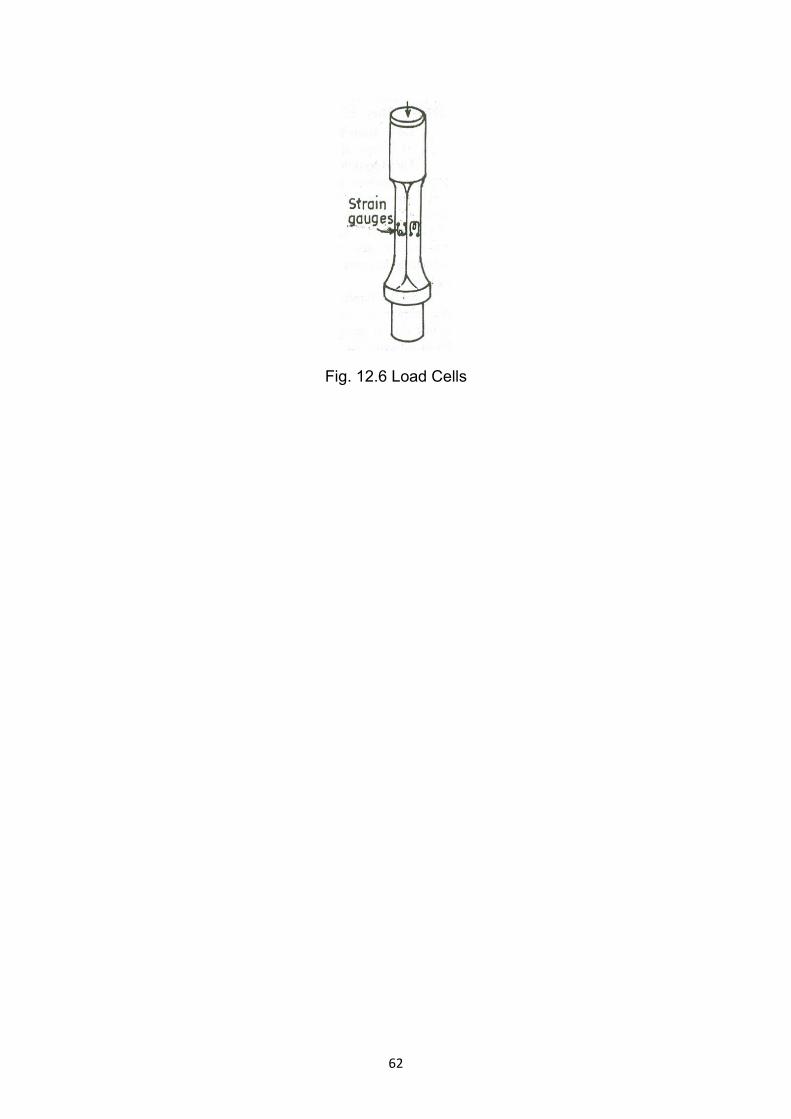
Fig. 12.6 Load Cells

62

LECTURE NO.13

PRESSURE SENSITIVE PRIMARY DEVICES: SOME OF THE COMMONLY USED FORCE SUMMING DEVICES, BOURDON TUBES, DIAPHRAGMS AND BELLOWS

PRESSURE SENSITIVE PRIMARY DEVICES

Most pressure measuring devices use elastic members for sensing

pressure at the primary stage. These elastic members are of many types and

convert the pressure into mechanical displacement which is later converted

into an electrical form using a secondary transducer. These devices are many a

time known as force summing devices. Fig. 13.1 shows some of the commonly

pressure sensitive primary devices

Fig. 13.1 Pressure sensitive primary devices

The principle of working of these devices is: the fluid whose pressure is

to be measured is made to press the pressure sensitive element and since the

element is an elastic member, it deflects causing a mechanical displacement.

The displacement is proportional to the pressure applied. The displacement is

then measured with the help of electrical transducers. The output of the

electrical transducers is proportional to the displacement and hence to the

applied input pressure.

Some of the commonly used force summing devices are,

63

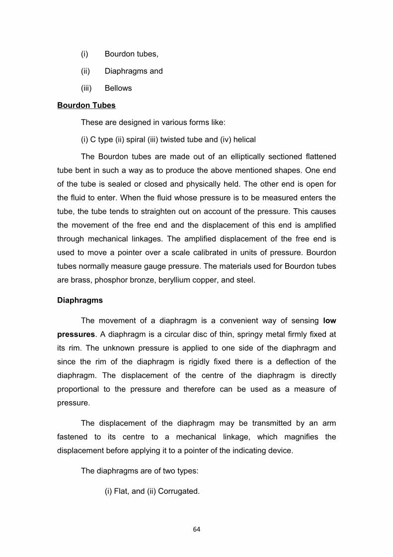
(i) Bourdon tubes,

(ii) Diaphragms and

(iii) Bellows

Bourdon Tubes

These are designed in various forms like:

(i) C type (ii) spiral (iii) twisted tube and (iv) helical

The Bourdon tubes are made out of an elliptically sectioned flattened

tube bent in such a way as to produce the above mentioned shapes. One end

of the tube is sealed or closed and physically held. The other end is open for

the fluid to enter. When the fluid whose pressure is to be measured enters the

tube, the tube tends to straighten out on account of the pressure. This causes

the movement of the free end and the displacement of this end is amplified

through mechanical linkages. The amplified displacement of the free end is

used to move a pointer over a scale calibrated in units of pressure. Bourdon

tubes normally measure gauge pressure. The materials used for Bourdon tubes

are brass, phosphor bronze, beryllium copper, and steel.

Diaphragms

The movement of a diaphragm is a convenient way of sensing low

pressures. A diaphragm is a circular disc of thin, springy metal firmly fixed at

its rim. The unknown pressure is applied to one side of the diaphragm and

since the rim of the diaphragm is rigidly fixed there is a deflection of the

diaphragm. The displacement of the centre of the diaphragm is directly

proportional to the pressure and therefore can be used as a measure of

pressure.

The displacement of the diaphragm may be transmitted by an arm

fastened to its centre to a mechanical linkage, which magnifies the

displacement before applying it to a pointer of the indicating device.

The diaphragms are of two types:

(i) Flat, and (ii) Corrugated.

64

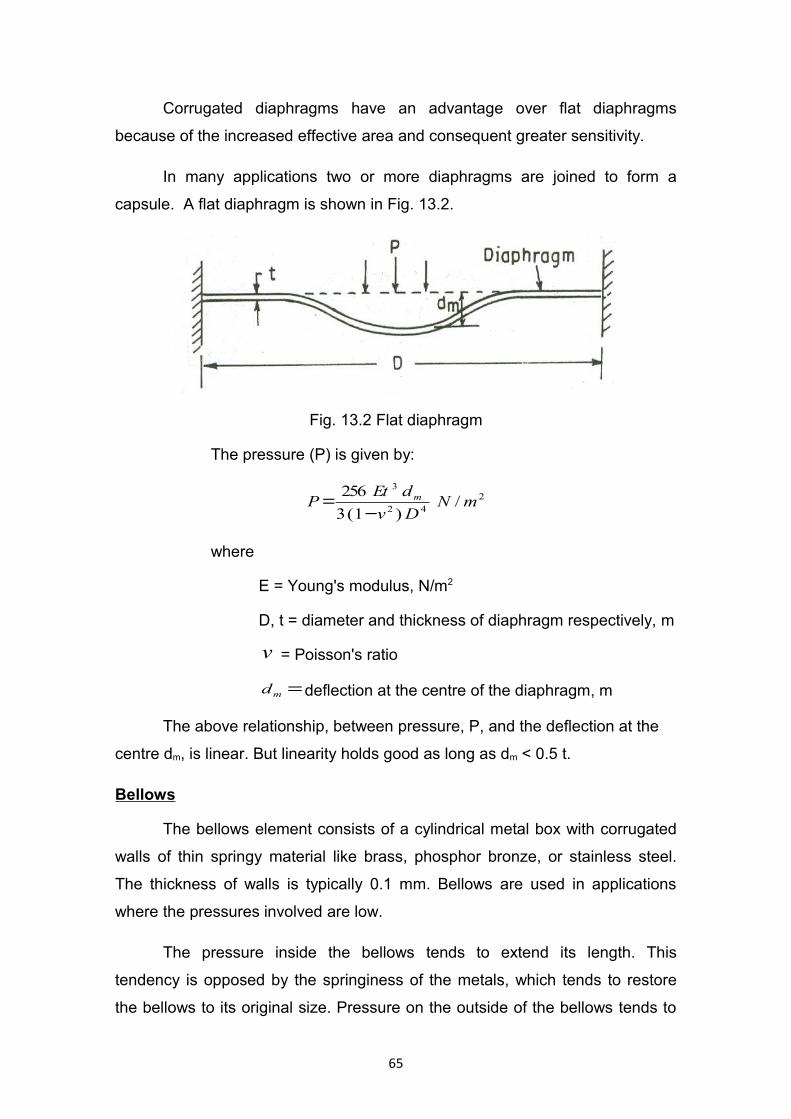
Corrugated diaphragms have an advantage over flat diaphragms

because of the increased effective area and consequent greater sensitivity.

In many applications two or more diaphragms are joined to form a

capsule. A flat diaphragm is shown in Fig. 13.2.

Fig. 13.2 Flat diaphragm

The pressure (P) is given by:

242

3

/)1(3

256mN

Dv

dEtP m

−=

where

E = Young's modulus, N/m2

D, t = diameter and thickness of diaphragm respectively, m

v = Poisson's ratio

=md deflection at the centre of the diaphragm, m

The above relationship, between pressure, P, and the deflection at the

centre dm, is linear. But linearity holds good as long as dm < 0.5 t.

Bellows

The bellows element consists of a cylindrical metal box with corrugated

walls of thin springy material like brass, phosphor bronze, or stainless steel.

The thickness of walls is typically 0.1 mm. Bellows are used in applications

where the pressures involved are low.

The pressure inside the bellows tends to extend its length. This

tendency is opposed by the springiness of the metals, which tends to restore

the bellows to its original size. Pressure on the outside of the bellows tends to

65

reduce its length and this tendency also, is opposed by the springiness of

metal. When the pressures are small the springiness of the metal sufficient.

However, when, the pressures are high, the springiness of the walls may not be

sufficient to restore the bellows to its original size. For such applications springs

are located inside the bellows to provide additional springiness to restore the

bellows to its original size.

The action of the bellows is as under:

The pressure to be measured is applied from the left end as shown in

Fig.13.1. The pressure inside the bellows extends its length. Since the left hand

end is fixed, there is a displacement of the right hand end to which a rod is

connected. The displacement of this rod is directly proportional to the pressure

inside the bellows. The displacement of the rod is small and may be amplified

by using mechanical linkage and then transferred to a pointer moving over a

calibrated scale.

66

LECTURE NO.14

TEMPERATURE MEASUREMENT: INTRODUCTION- TEMPERATURE SCALES- INTERNATIONAL PRACTICAL TEMPERATURE SCALE (IPTS)

INTRODUCTIONTemperature is a very widely measured and frequently controlled

variable used in numerous industrial applications. In general, chemical

reactions in the industrial processes and products are temperature dependent

and the desired quality of a product is possible only if the temperature is

accurately measured and maintained. In the heat treatment of steel and

aluminum alloys, temperature measurement and control plays a crucial role in

incorporating the desired material properties in the finished heat-treated

products. The other areas where measurement and control of temperature is

essential are: plastic manufacturing, nuclear reactor components, milk and

dairy products, plant furnace and molten metals, heating and air-conditioning

systems, space shuttle components, blades of gas turbines, etc.

The temperature is defined as the degree of hotness or coldness of a

body or an environment measured on a definite scale. Definition of temperature

is also defined based on its equivalence to a driving force or potential that

caused the flow of energy as heat. Thus, we can define temperature as a

condition of a body by virtue of which heat is transferred to or from other

bodies.

It may be noted that there is a difference between the quantities

temperature and heat. Temperature may be defined as 'degree' of heat

whereas heat is taken to mean as 'quantity' of heat. For example, a bucket of

warm water would melt more ice than a small spoon of boiling water. The warm

water in the bucket obviously contains greater quantity of heat than that in the

spoon containing boiling water. But its temperature is lower than the boiling

water, a fact that is readily apparent if a finger is dipped in both the

vessels.

Temperature is a fundamental quantity, much the same way as mass,

length and time. The law that is used in temperature measurement is known as

the Zeroth law of thermodynamics.

67

Zeroth law of thermodynamics

Zeroth law of thermodynamics states that if two bodies are in thermal

equilibrium with a third body, then they are all in thermal equilibrium with each

other.

TEMPERATURE SCALES

Two temperature scales in common use are the Fahrenheit and

Celsius scales. These scales are based on a specification of the number of

increments between freezing point and boiling point of water at the

standard atmospheric temperature.

The Celsius scale has 100 units between these points, while the

Fahrenheit scale has 180 units. The Celsius scale is currently more in use

because of the adoption of metric units. However, the absolute temperature

scale based on the thermodynamic ideal Carnot cycle has been correlated with

the Celsius and Fahrenheit scales as follows:

K (Absolute temperature, Kelvin scale) = °C + 273.15

where

°C is temperature on Celsius scale.

R (Absolute temperature, Rankine scale) = °F + 459.69

where

°F is the temperature on the Fahrenheit scale.

The zero points on both the scales represent the same physical state

and the ratio of two values is the same, regardless of the absolute scale used

i.e.

KelvinRankineT

T

T

T

=

1

2

1

2

The boiling and freezing points of water at a pressure of one atmosphere

(101.3 kN / m2) are taken as 100° and 0° on the Celsius scale and 212° and

68

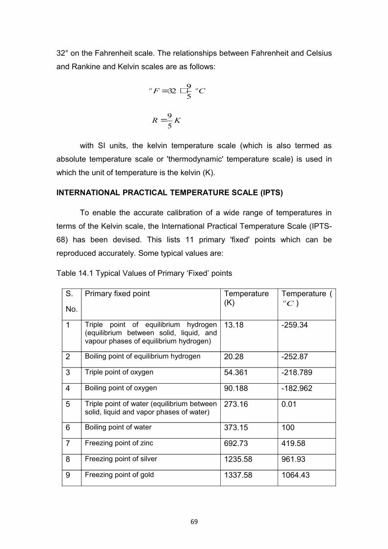
32° on the Fahrenheit scale. The relationships between Fahrenheit and Celsius

and Rankine and Kelvin scales are as follows:

CF oo

5

932 +=

KR5

9=

with SI units, the kelvin temperature scale (which is also termed as

absolute temperature scale or 'thermodynamic' temperature scale) is used in

which the unit of temperature is the kelvin (K).

INTERNATIONAL PRACTICAL TEMPERATURE SCALE (IPTS)

To enable the accurate calibration of a wide range of temperatures in

terms of the Kelvin scale, the International Practical Temperature Scale (IPTS-

68) has been devised. This lists 11 primary 'fixed' points which can be

reproduced accurately. Some typical values are:

Table 14.1 Typical Values of Primary ‘Fixed’ points

S.

No.

Primary fixed point Temperature (K)

Temperature (Co )

1 Triple point of equilibrium hydrogen (equilibrium between solid, liquid, and vapour phases of equilibrium hydrogen)

13.18 -259.34

2 Boiling point of equilibrium hydrogen 20.28 -252.87

3 Triple point of oxygen 54.361 -218.789

4 Boiling point of oxygen 90.188 -182.962

5 Triple point of water (equilibrium between solid, liquid and vapor phases of water)

273.16 0.01

6 Boiling point of water 373.15 100

7 Freezing point of zinc 692.73 419.58

8 Freezing point of silver 1235.58 961.93

9 Freezing point of gold 1337.58 1064.43

69

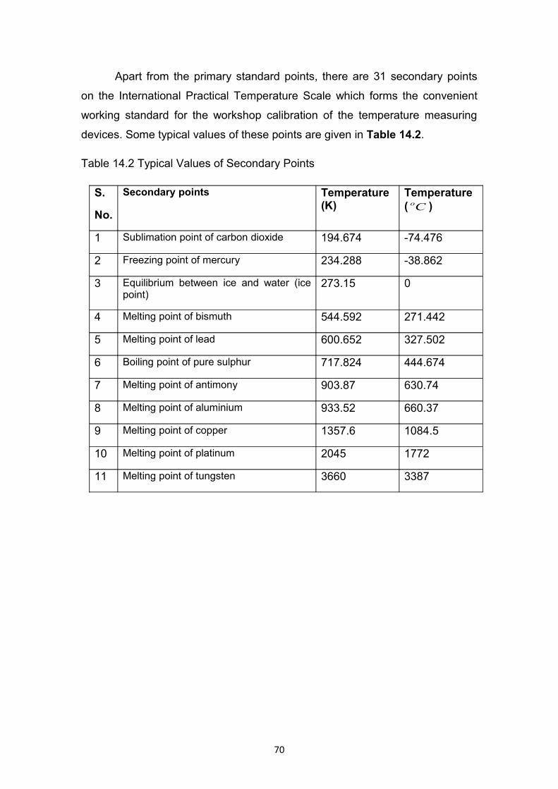
Apart from the primary standard points, there are 31 secondary points

on the International Practical Temperature Scale which forms the convenient

working standard for the workshop calibration of the temperature measuring

devices. Some typical values of these points are given in Table 14.2.

Table 14.2 Typical Values of Secondary Points

S.

No.

Secondary points Temperature (K)

Temperature ( Co )

1 Sublimation point of carbon dioxide 194.674 -74.476

2 Freezing point of mercury 234.288 -38.862

3 Equilibrium between ice and water (ice point)

273.15 0

4 Melting point of bismuth 544.592 271.442

5 Melting point of lead 600.652 327.502

6 Boiling point of pure sulphur 717.824 444.674

7 Melting point of antimony 903.87 630.74

8 Melting point of aluminium 933.52 660.37

9 Melting point of copper 1357.6 1084.5

10 Melting point of platinum 2045 1772

11 Melting point of tungsten 3660 3387

70

LECTURE NO.15

MEASUREMENT OF TEMPERATURE: CLASSIFICATION OF TEMPERATURE MEASURING DEVICES - BIMETALLIC THERMOMETERS - GLASS THERMOMETERS AND PRESSURE GAUGE THERMOMETERS - THERMOCOUPLES

MEASUREMENT OF TEMPERATURE

Temperature is measured by observing the effect that temperature

variation causes on the measuring device. Temperature measurement methods

can be broadly classified as follows:

1. non-electrical methods,

2. electrical methods, and

3. radiation methods.

NON-ELECTRICAL METHODS

The non-electrical methods of temperature measurement can be based

on anyone of the following principles:

1. change in the physical state,

2. change in the chemical properties, and

3. change in the physical properties.

BIMETALLIC THERMOMETER

This type of thermometer also employs the principle of solid expansion

and consists of a 'bimetal' strip usually in the form of a cantilever beam

[Fig.15.1 (a)]. This comprises strips of two metals, having different coefficients

of thermal expansion, welded or riveted together so that relative motion

between them is prevented. An increase in temperature causes the deflection

of the free end of the strip as shown in Fig.15.1 (b), assuming that metal A has

the higher coefficient of expansion. The deflection with the temperature is

nearly linear, depending mainly on the coefficient of linear thermal expansion.

Invar is commonly employed as the low expansion metal. This is an iron-

nickel alloy containing 36% nickel. Its coefficient of thermal expansion is around

71

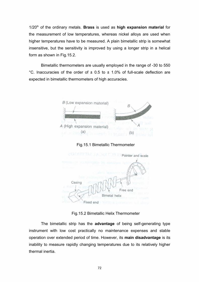
1/20th of the ordinary metals. Brass is used as high expansion material for

the measurement of low temperatures, whereas nickel alloys are used when

higher temperatures have to be measured. A plain bimetallic strip is somewhat

insensitive, but the sensitivity is improved by using a longer strip in a helical

form as shown in Fig.15.2.

Bimetallic thermometers are usually employed in the range of -30 to 550

°C. Inaccuracies of the order of ± 0.5 to ± 1.0% of full-scale deflection are

expected in bimetallic thermometers of high accuracies.

Fig.15.1 Bimetallic Thermometer

Fig.15.2 Bimetallic Helix Thermometer

The bimetallic strip has the advantage of being self-generating type

instrument with low cost practically no maintenance expenses and stable

operation over extended period of time. However, its main disadvantage is its

inability to measure rapidly changing temperatures due to its relatively higher

thermal inertia.

72

LIQUID-IN-GLASS THERMOMETER/MERCURY-IN-GLASS THERMOMETER

The liquid-in-glass thermometer is one of the most common temperature

measuring devices. Both liquid and glass expand on heating and their

differential expansion is used to indicate the temperature. The lower

temperature limit is -37.8 ºC for mercury, down to –130 °C for pentane. The

higher temperature range is 340 °C (boiling point of mercury is 357 °C ) but this

range may be extended to 560 °C C by filling the space above mercury with

CO2 or N2 at high pressure, thereby increasing its boiling point and range. The

precision of the thermometer depends on the care used in calibration. A typical

instrument is checked and marked from two to five reference temperatures.

Intermediate points are marked by interpolation. The calibration of the

thermometer should be occasionally checked against the ice point to take into

account the aging effects. Precision thermometers are sometimes marked for

partial or total immersion and also for horizontal or vertical orientation. The

accuracy of these thermometers does not exceed 0.1°C. However, when

increased accuracy is required, a Beckmann range thermometer can be

used. It contains a big bulb attached to a very fine capillary. The range of the

thermometer is limited to 5 – 6 °C with an accuracy of 0.005°C.

Liquid-in-glass thermometers have notable qualities like low cost,

simplicity in use, portability and convenient visual indication without the use of

any external power. However, their use is limited to certain laboratory

applications. It is not preferred in industrial applications because of its fragility

and its lack of adaptability to remote indication. Further, it introduces time

lag in the measurement of dynamic signals because of relatively high heat

capacity of the bulb.

PRESSURE THERMOMETERS / PRESSURE SPRING THERMOMETERS

Pressure thermometer is based on the principle of fluid expansion due to

an increase in the pressure in a given volume of the temperature measuring

system. It is one of the most economical, versatile and widely used devices in

industrial temperature measurements. It has a relatively large metal bulb (often

stainless steel) instead of glass. This results in a robust, easy-to-read

thermometer that may be read remotely by connecting the bulb to a Bourdon

73

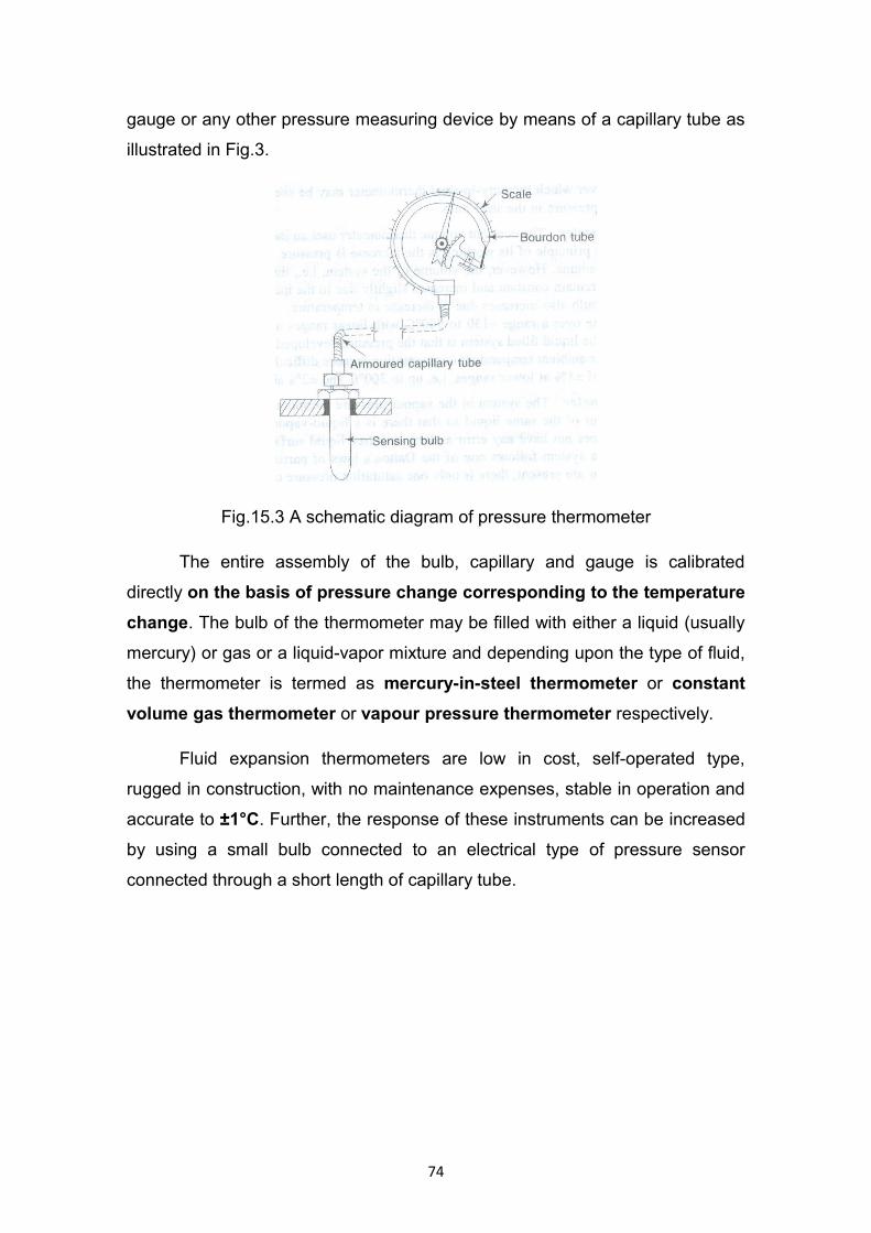
gauge or any other pressure measuring device by means of a capillary tube as

illustrated in Fig.3.

Fig.15.3 A schematic diagram of pressure thermometer

The entire assembly of the bulb, capillary and gauge is calibrated

directly on the basis of pressure change corresponding to the temperature

change. The bulb of the thermometer may be filled with either a liquid (usually

mercury) or gas or a liquid-vapor mixture and depending upon the type of fluid,

the thermometer is termed as mercury-in-steel thermometer or constant

volume gas thermometer or vapour pressure thermometer respectively.

Fluid expansion thermometers are low in cost, self-operated type,

rugged in construction, with no maintenance expenses, stable in operation and

accurate to ±1°C. Further, the response of these instruments can be increased

by using a small bulb connected to an electrical type of pressure sensor

connected through a short length of capillary tube.

74

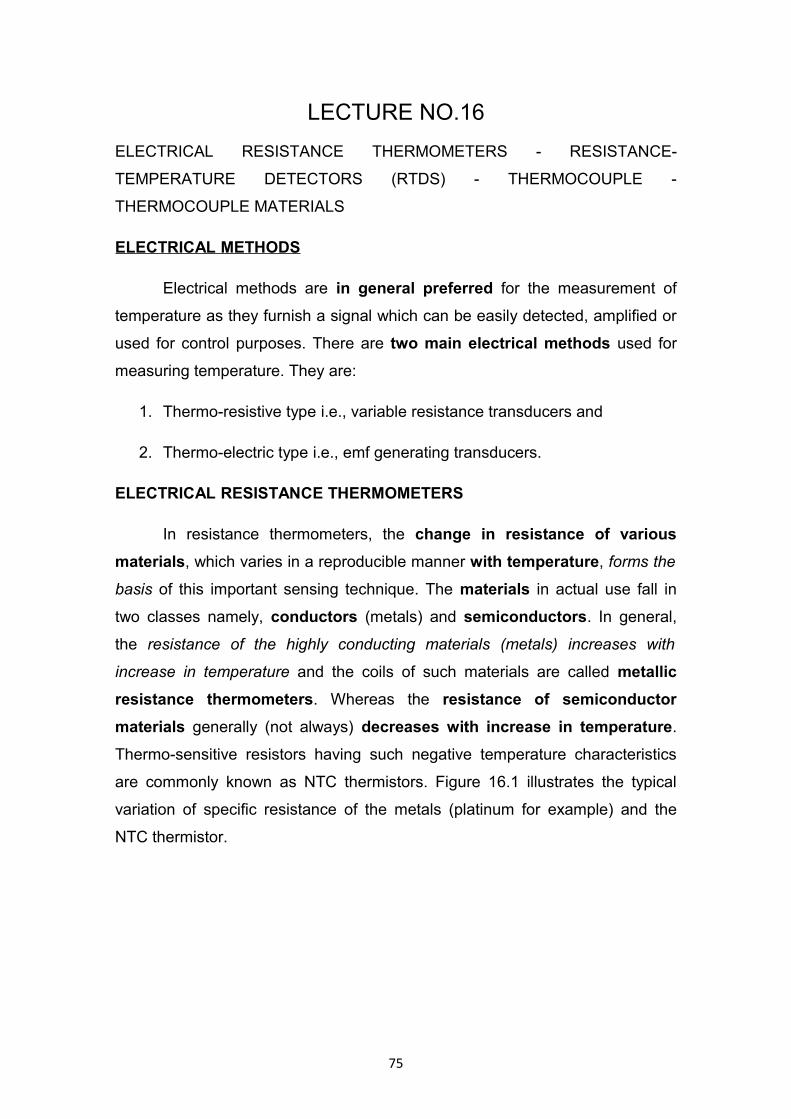
LECTURE NO.16

ELECTRICAL RESISTANCE THERMOMETERS - RESISTANCE-

TEMPERATURE DETECTORS (RTDS) - THERMOCOUPLE -

THERMOCOUPLE MATERIALS

ELECTRICAL METHODS

Electrical methods are in general preferred for the measurement of

temperature as they furnish a signal which can be easily detected, amplified or

used for control purposes. There are two main electrical methods used for

measuring temperature. They are:

1. Thermo-resistive type i.e., variable resistance transducers and

2. Thermo-electric type i.e., emf generating transducers.

ELECTRICAL RESISTANCE THERMOMETERS

In resistance thermometers, the change in resistance of various

materials, which varies in a reproducible manner with temperature, forms the

basis of this important sensing technique. The materials in actual use fall in

two classes namely, conductors (metals) and semiconductors. In general,

the resistance of the highly conducting materials (metals) increases with

increase in temperature and the coils of such materials are called metallic

resistance thermometers. Whereas the resistance of semiconductor

materials generally (not always) decreases with increase in temperature.

Thermo-sensitive resistors having such negative temperature characteristics

are commonly known as NTC thermistors. Figure 16.1 illustrates the typical

variation of specific resistance of the metals (platinum for example) and the

NTC thermistor.

75

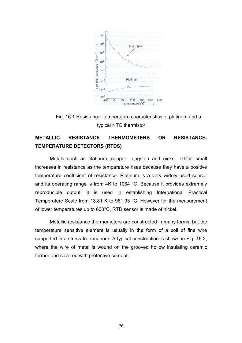
Fig. 16.1 Resistance- temperature characteristics of platinum and a

typical NTC thermistor

METALLIC RESISTANCE THERMOMETERS OR RESISTANCE-

TEMPERATURE DETECTORS (RTDS)

Metals such as platinum, copper, tungsten and nickel exhibit small

increases in resistance as the temperature rises because they have a positive

temperature coefficient of resistance. Platinum is a very widely used sensor

and its operating range is from 4K to 1064 °C. Because it provides extremely

reproducible output, it is used in establishing International Practical

Temperature Scale from 13.81 K to 961.93 °C. However for the measurement

of lower temperatures up to 600°C, RTD sensor is made of nickel.

Metallic resistance thermometers are constructed in many forms, but the

temperature sensitive element is usually in the form of a coil of fine wire

supported in a stress-free manner. A typical construction is shown in Fig. 16.2,

where the wire of metal is wound on the grooved hollow insulating ceramic

former and covered with protective cement.

76

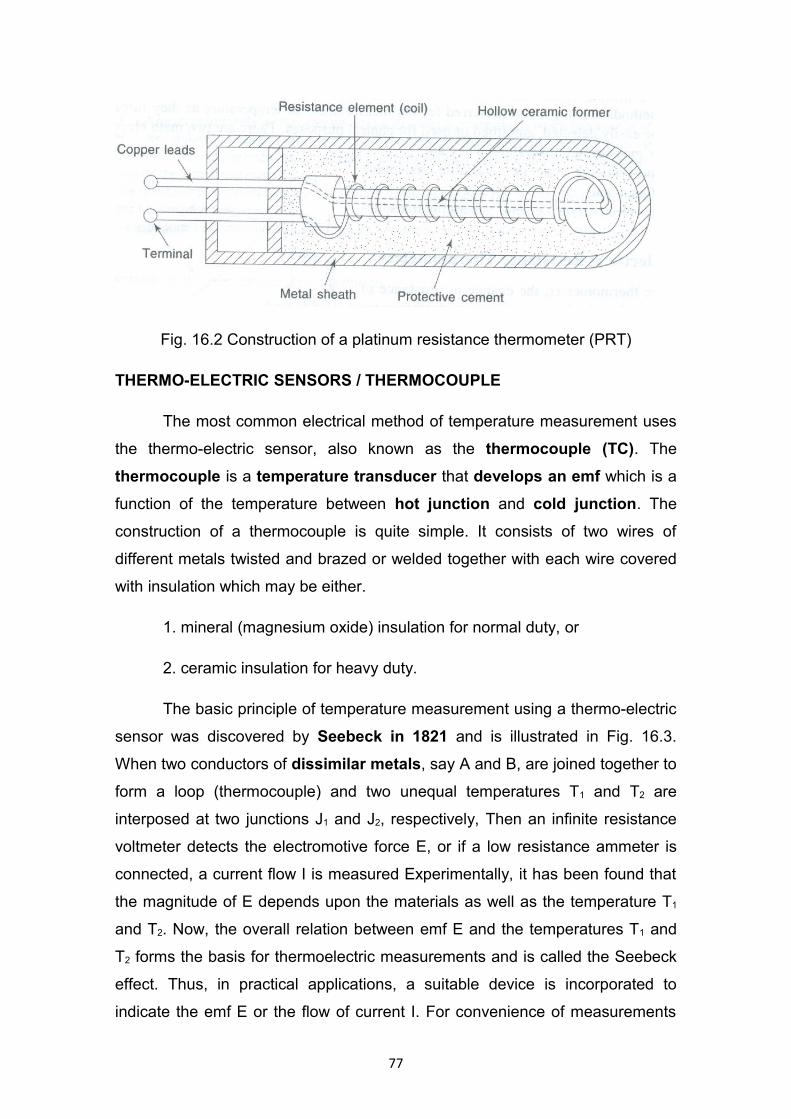
Fig. 16.2 Construction of a platinum resistance thermometer (PRT)

THERMO-ELECTRIC SENSORS / THERMOCOUPLE

The most common electrical method of temperature measurement uses

the thermo-electric sensor, also known as the thermocouple (TC). The

thermocouple is a temperature transducer that develops an emf which is a

function of the temperature between hot junction and cold junction. The

construction of a thermocouple is quite simple. It consists of two wires of

different metals twisted and brazed or welded together with each wire covered

with insulation which may be either.

1. mineral (magnesium oxide) insulation for normal duty, or

2. ceramic insulation for heavy duty.

The basic principle of temperature measurement using a thermo-electric

sensor was discovered by Seebeck in 1821 and is illustrated in Fig. 16.3.

When two conductors of dissimilar metals, say A and B, are joined together to

form a loop (thermocouple) and two unequal temperatures T1 and T2 are

interposed at two junctions J1 and J2, respectively, Then an infinite resistance

voltmeter detects the electromotive force E, or if a low resistance ammeter is

connected, a current flow I is measured Experimentally, it has been found that

the magnitude of E depends upon the materials as well as the temperature T1

and T2. Now, the overall relation between emf E and the temperatures T1 and

T2 forms the basis for thermoelectric measurements and is called the Seebeck

effect. Thus, in practical applications, a suitable device is incorporated to

indicate the emf E or the flow of current I. For convenience of measurements

77

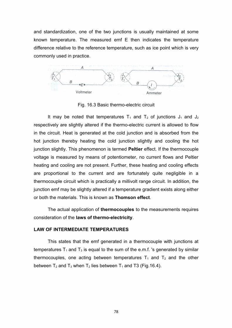
and standardization, one of the two junctions is usually maintained at some

known temperature. The measured emf E then indicates the temperature

difference relative to the reference temperature, such as ice point which is very

commonly used in practice.

Fig. 16.3 Basic thermo-electric circuit

It may be noted that temperatures T1 and T2 of junctions J1 and J2

respectively are slightly altered if the thermo-electric current is allowed to flow

in the circuit. Heat is generated at the cold junction and is absorbed from the

hot junction thereby heating the cold junction slightly and cooling the hot

junction slightly. This phenomenon is termed Peltier effect. If the thermocouple

voltage is measured by means of potentiometer, no current flows and Peltier

heating and cooling are not present. Further, these heating and cooling effects

are proportional to the current and are fortunately quite negligible in a

thermocouple circuit which is practically a millivolt range circuit. In addition, the

junction emf may be slightly altered if a temperature gradient exists along either

or both the materials. This is known as Thomson effect.

The actual application of thermocouples to the measurements requires

consideration of the laws of thermo-electricity.

LAW OF INTERMEDIATE TEMPERATURES

This states that the emf generated in a thermocouple with junctions at

temperatures T1 and T3 is equal to the sum of the e.m.f. 's generated by similar

thermocouples, one acting between temperatures T1 and T2 and the other

between T2 and T3 when T2 lies between T1 and T3 (Fig.16.4).

78

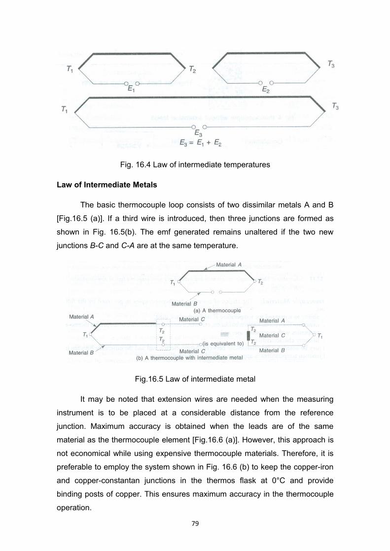
Fig. 16.4 Law of intermediate temperatures

Law of Intermediate Metals

The basic thermocouple loop consists of two dissimilar metals A and B

[Fig.16.5 (a)]. If a third wire is introduced, then three junctions are formed as

shown in Fig. 16.5(b). The emf generated remains unaltered if the two new

junctions B-C and C-A are at the same temperature.

Fig.16.5 Law of intermediate metal

It may be noted that extension wires are needed when the measuring

instrument is to be placed at a considerable distance from the reference

junction. Maximum accuracy is obtained when the leads are of the same

material as the thermocouple element [Fig.16.6 (a)]. However, this approach is

not economical while using expensive thermocouple materials. Therefore, it is

preferable to employ the system shown in Fig. 16.6 (b) to keep the copper-iron

and copper-constantan junctions in the thermos flask at 0°C and provide

binding posts of copper. This ensures maximum accuracy in the thermocouple

operation.

79

(a) A thermocouple without extension leads

(b) Conventional method of establishing reference function temperature with

copper extension leads

Fig.16.6 Schematics of Thermocouple circuits with and without extension leads

in a typical iron-constantan thermocouple circuit

(a) A thermocouple without extension leads

(b) Conventional method of establishing reference function temperature with copper extension leads

THERMOCOUPLE MATERIALS

The choice of materials for thermocouples in governed by the following

factors:

1. Ability to withstand the temperature, at which they are used,

80

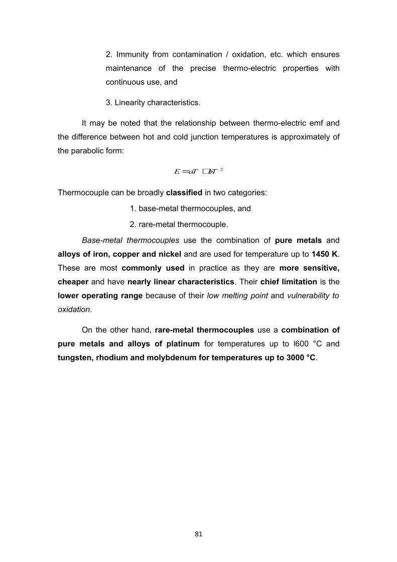
2. Immunity from contamination / oxidation, etc. which ensures

maintenance of the precise thermo-electric properties with

continuous use, and

3. Linearity characteristics.

It may be noted that the relationship between thermo-electric emf and

the difference between hot and cold junction temperatures is approximately of

the parabolic form:

2bTaTE +=

Thermocouple can be broadly classified in two categories:

1. base-metal thermocouples, and

2. rare-metal thermocouple.

Base-metal thermocouples use the combination of pure metals and

alloys of iron, copper and nickel and are used for temperature up to 1450 K.

These are most commonly used in practice as they are more sensitive,

cheaper and have nearly linear characteristics. Their chief limitation is the

lower operating range because of their low melting point and vulnerability to

oxidation.

On the other hand, rare-metal thermocouples use a combination of

pure metals and alloys of platinum for temperatures up to l600 °C and

tungsten, rhodium and molybdenum for temperatures up to 3000 °C.

81

LECTURE NO.17

PRESSURE - GAUGE PRESSURE, ABSOLUTE PRESSURE,

DIFFERENTIAL PRESSURE, VACUUM - UNITS OF PRESSURE -

PRESSURE SCALES - CONVERSION OF UNITS- TYPES OF PRESSURE

MEASUREMENT DEVICES

PRESSURE MEASUREMENT

INTRODUCTION

Pressure means force per unit area, exerted by a fluid on the surface of

the container.

Pressure measurements are one of the most important measurements

made in industry especially in continuous process industries such as chemical

processing, food and manufacturing. The principles used in measurement of

pressure are also applied in the measurement of temperature, flow and liquid

level.

Pressure is represented as force per unit area.

Fluid pressure is on account of exchange of momentum between the molecules

of the fluid and a container wall.

Static and Dynamic Pressures

When a fluid is in equilibrium, the pressure at a point is identical in all

directions and is independent of orientation. This is called static pressure.

However, when pressure gradients occur within a continuum (field) of

pressure, the attempt to restore equilibrium results in fluid flow from regions of

higher pressure to regions of lower pressure. In this case the pressures are no

longer independent of direction and are called dynamic pressures.

Velocity and Impact Pressures

Pressure components of different nature exist in a flowing fluid. For

example, in case a small tube or probe for sampling, it is found that the results

depend upon how the tube is oriented. In case, the tube or probe is so aligned

that there is a direct impact of flow on the opening of the tube or probe as

shown in Fig.17.1 (a) it senses a total or stagnation pressure. If the tube or

probe is oriented as shown in Fig.17.1 (b), the results are different and what we

82

obtain is called static pressure.

Fig.17.1 Impact and Static Pressure tubes

Static Pressure

Static pressure is considered as the pressure that is experienced if

moving along the stream and the total pressure may be defined as the pressure

if the stream is brought to rest is entropically. The difference of the two

pressures is the pressure due to fluid motion commonly referred as the velocity

pressure.

pressure static - pressure (total) stagnation pressureVelocity =

Therefore, in order to properly interpret flow measurements,

consideration must be given how the pressure is being measured.

Absolute pressure.

Absolute pressure means the fluid pressure above the reference value

of a perfect vacuum or the absolute zero pressure.

Gauge pressure.

It represents the difference between the absolute pressure and the local

atmospheric pressure.

Vacuum

Vacuum on the other hand, represents the amount by which

atmospheric pressure exceeds the absolute pressure.

83

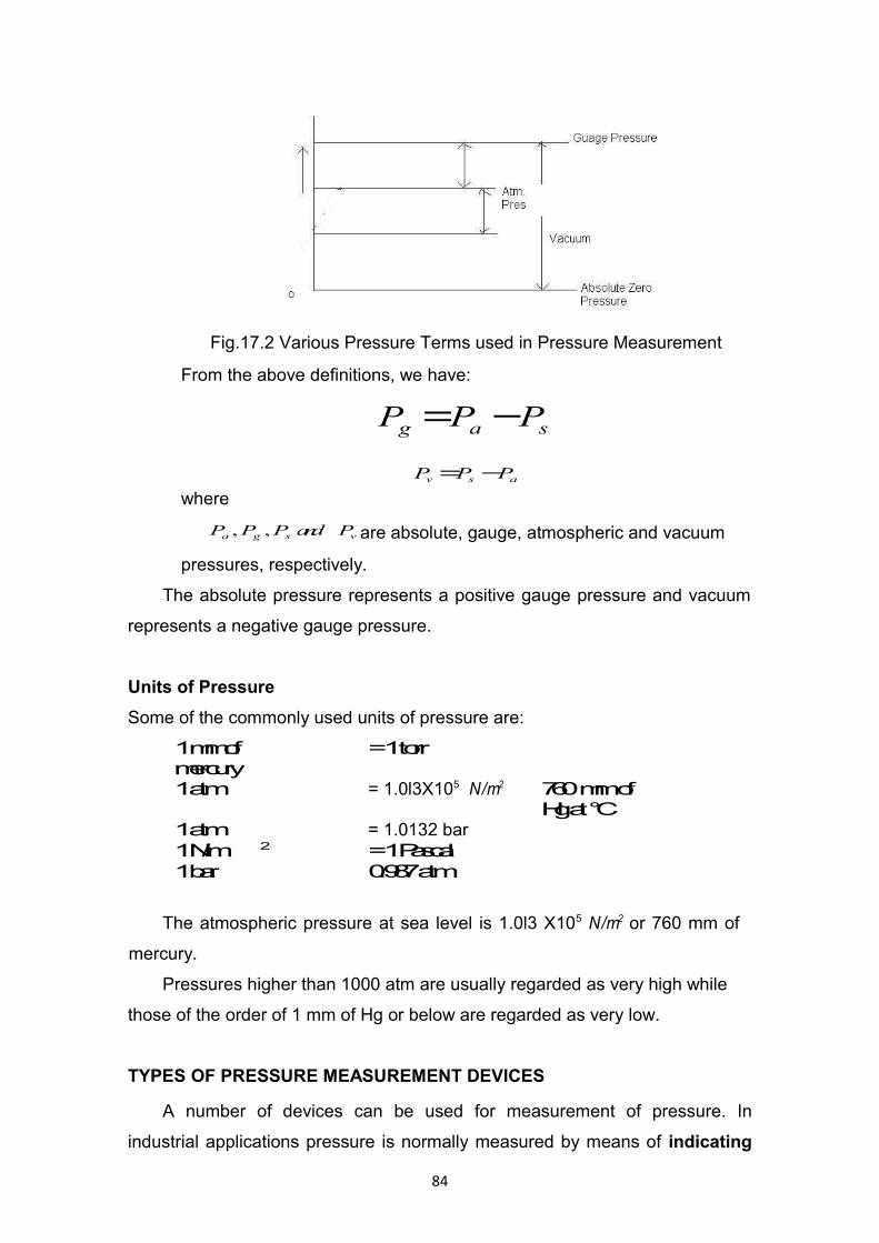
Fig.17.2 Various Pressure Terms used in Pressure Measurement

From the above definitions, we have:

sag PPP −=

asv PPP −=

where

vsga PandPPP ,, are absolute, gauge, atmospheric and vacuum

pressures, respectively.

The absolute pressure represents a positive gauge pressure and vacuum

represents a negative gauge pressure.

Units of Pressure

Some of the commonly used units of pressure are:

1 mm of mercury

= 1 torr

1 atm = 1.0l3X105 N/m2 760 mm of Hg at °C

1 atm = 1.0132 bar1 N/m 2 = 1 Pascal1 bar 0.987 atm

The atmospheric pressure at sea level is 1.0l3 X105 N/m2 or 760 mm of

mercury.

Pressures higher than 1000 atm are usually regarded as very high while

those of the order of 1 mm of Hg or below are regarded as very low.

TYPES OF PRESSURE MEASUREMENT DEVICES

A number of devices can be used for measurement of pressure. In

industrial applications pressure is normally measured by means of indicating

84

gauges and recorders. These instruments are

mechanical,

electromechanical

electrical or electronic in operation

(i) Mechanical Pressure Measuring Instruments.

Pressure can be easily transduced to force by allowing it to act on a

known area. Therefore, basic methods of measuring force and pressure are

essentially the same except for the pressures in the high vacuum region.

Mechanical instruments used for pressure measurement are based on

comparison with known dead weights acting on known areas or on the

deflection of elastic elements subjected to unknown pressures.

Instruments using this principle include manometers. And the elastic

members used are Bourdon tubes, bellows and diaphragms.

(ii) Electromechanical Instruments. These instruments generally employ

mechanical means for detecting pressure and electrical means for indicating or

recording pressure. Electromechanical instruments are very well suitable for

dynamic measurements as they have an excellent frequency response

characteristics.

(iii) Electronic Instruments. These pressure measuring instruments normally

depend on some physical change that can be detected and indicated or

recorded through electronic means. These instruments are used for vacuum

measurements.

85

LECTURE NO.18

MEASUREMENT OF PRESSURE: MANOMETERS - U TUBE MANOMETER -

INCLINED TUBE MANOMETER - WELL TYPE MANOMETER - PROPERTIES

OF MANOMETRIC FLUIDS

MANOMETERS

Manometers measure the unknown pressures by balancing against the

gravitational force of liquid heads. Manometers are self-balancing deflection

type of instruments and have continuous rather than stepwise output. These

are used in plant systems, as differential pressure devices. They are used as

primary standards for pressure measurements from low vacuum range to about

0.1 MN/m2.

Construction of Manometers. Manometer bodies are usually made of brass,

steel, aluminum or stainless steel. Tubes are made of pyrex. Scales are

provided which read pressures in terms of mm of water or in mm of mercury.

They can be provided to read in terms of kN/m2 (kPa).

Types of Manometers

The various types of manometers are:

U tube manometer, Well type Manometer, Inclined tube Manometer.

U tube manometer

The U tube manometer is shown in Fig. 18.1. This is used for

measurement of liquid or gas pressures. The manometer is filled with a

manometric fluid whose specific gravity is known. The difference between the

pressures on two limbs of the manometer is a function of h (the difference

between the levels of the manometric fluid in the two limbs).

86

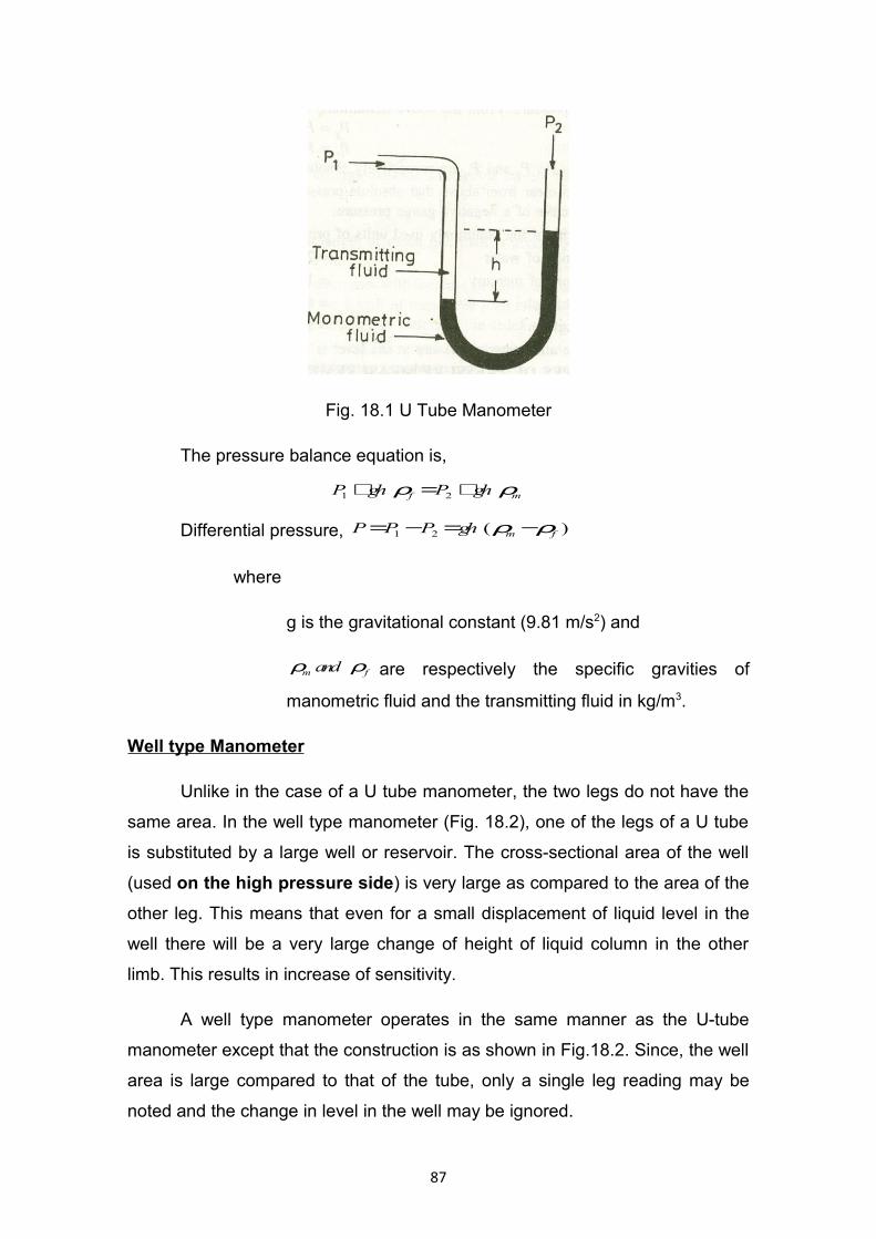
Fig. 18.1 U Tube Manometer

The pressure balance equation is,

mf ghPghP ρρ +=+ 21

Differential pressure, )(21 fmghPPP ρρ −=−=

where

g is the gravitational constant (9.81 m/s2) and

fm and ρρ are respectively the specific gravities of

manometric fluid and the transmitting fluid in kg/m3.

Well type Manometer

Unlike in the case of a U tube manometer, the two legs do not have the

same area. In the well type manometer (Fig. 18.2), one of the legs of a U tube

is substituted by a large well or reservoir. The cross-sectional area of the well

(used on the high pressure side) is very large as compared to the area of the

other leg. This means that even for a small displacement of liquid level in the

well there will be a very large change of height of liquid column in the other

limb. This results in increase of sensitivity.

A well type manometer operates in the same manner as the U-tube

manometer except that the construction is as shown in Fig.18.2. Since, the well

area is large compared to that of the tube, only a single leg reading may be

noted and the change in level in the well may be ignored.

87

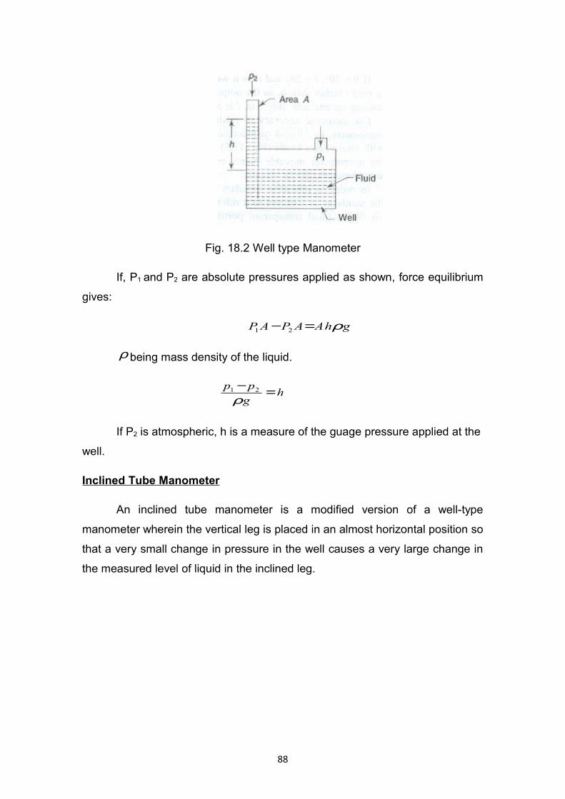
Fig. 18.2 Well type Manometer

If, P1 and P2 are absolute pressures applied as shown, force equilibrium

gives:

ghAAPAP ρ=− 21

ρ being mass density of the liquid.

hg

pp =−ρ

21

If P2 is atmospheric, h is a measure of the guage pressure applied at the

well.

Inclined Tube Manometer

An inclined tube manometer is a modified version of a well-type

manometer wherein the vertical leg is placed in an almost horizontal position so

that a very small change in pressure in the well causes a very large change in

the measured level of liquid in the inclined leg.

88

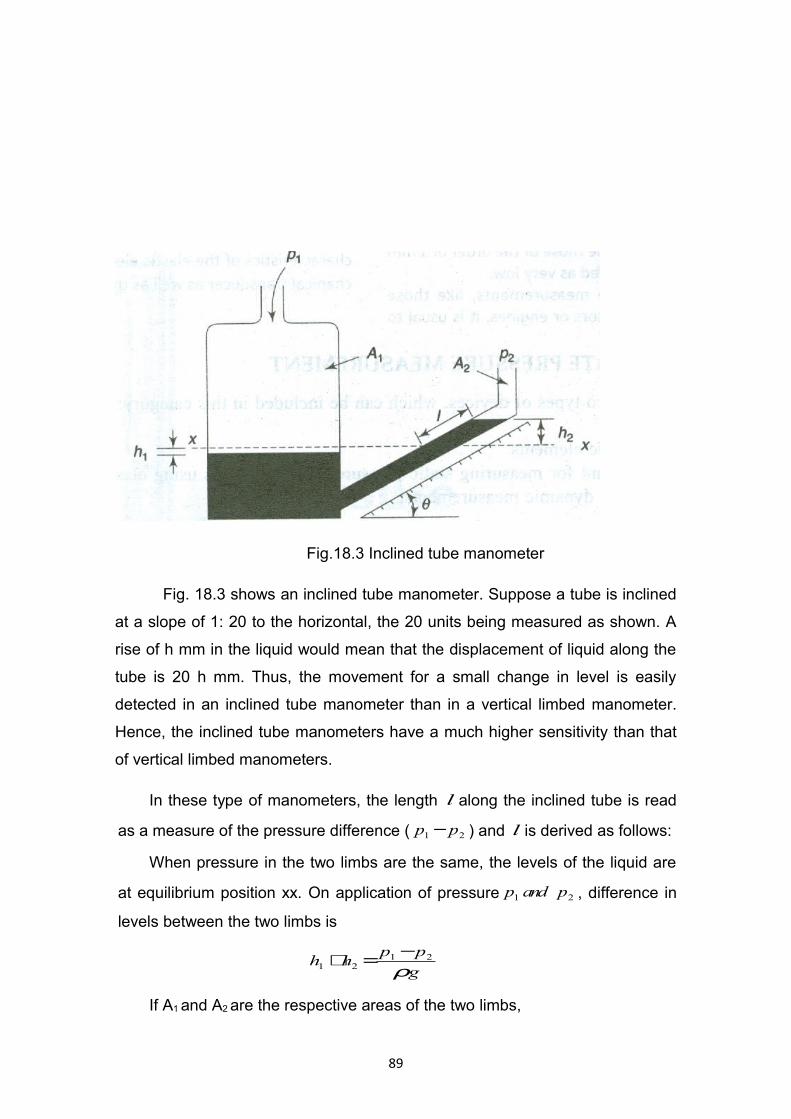
Fig.18.3 Inclined tube manometer

Fig. 18.3 shows an inclined tube manometer. Suppose a tube is inclined

at a slope of 1: 20 to the horizontal, the 20 units being measured as shown. A

rise of h mm in the liquid would mean that the displacement of liquid along the

tube is 20 h mm. Thus, the movement for a small change in level is easily

detected in an inclined tube manometer than in a vertical limbed manometer.

Hence, the inclined tube manometers have a much higher sensitivity than that

of vertical limbed manometers.

In these type of manometers, the length l along the inclined tube is read

as a measure of the pressure difference ( 21 pp − ) and l is derived as follows:

When pressure in the two limbs are the same, the levels of the liquid are

at equilibrium position xx. On application of pressure 21 pandp , difference in

levels between the two limbs is

g

pphh

ρ21

21

−=+

If A1 and A2 are the respective areas of the two limbs,

89

lAhA 211 =

θsin2 lh =

From the above equations,

+=− θρ sin

1

221 A

Aglpp

If 1221 / AAorAA >> is negligible,

221 sin ghglpp ρθρ ==−

If 20 2,30 hl ==θ and thus it would be more accurate to read l rather

than 2h as the output. Since ,21 AA >> the reading on one side only, viz. l is

required.

Properties of Manometric Fluids

The desirable properties of manometric fluids are:

i. Low viscosity: Fluids with low viscosity give quick response.

ii. Low co-efficient of thermal expansion: The value of measured pressure

is affected by changes in density of manometreric fluids which is

dependent upon temperature.

iii. Low vapor pressure, negligible surface tension, and low capillary effects,

and non-sticky effects.

iv. Non-corrosive, non-poisoness

v. Long term stability

Some of the manometric fluids are: water, Mercury, transformer oil

(suitable for ammonia gas flow meters and measurements of small pressure

differences), Aniline (suitable for low pressure air or gas flow meters with the

exception of ammonia and chlorine)

Advantages of Manometers.

i. The advantages of manometers are:

ii. They are simple in construction, high accuracy, and good repeatability.

iii. Wide range of manometric fluids can be used

90

iv. They can be used both as measuring instruments and also as primary

standards for pressure measurement on account of their inherent

accuracy.

v. The accuracy level of manometers is quite good.

Disadvantages of Manometers.

The disadvantages of manometers are:

i. They are fragile in construction and hence lack portability.

ii. When visual reading of height h is used, corrections must be applied for

effect of temperature on the engraved (fixed) scale.

iii. The value of gravitational constant g is dependent upon the altitude of

the place

iv. Accurate leveling is required in order to have good accuracy.

v. Poor dynamic response.

Several types of modified manometers are available which have the

advantages of ease in use and high sensitivity.

91

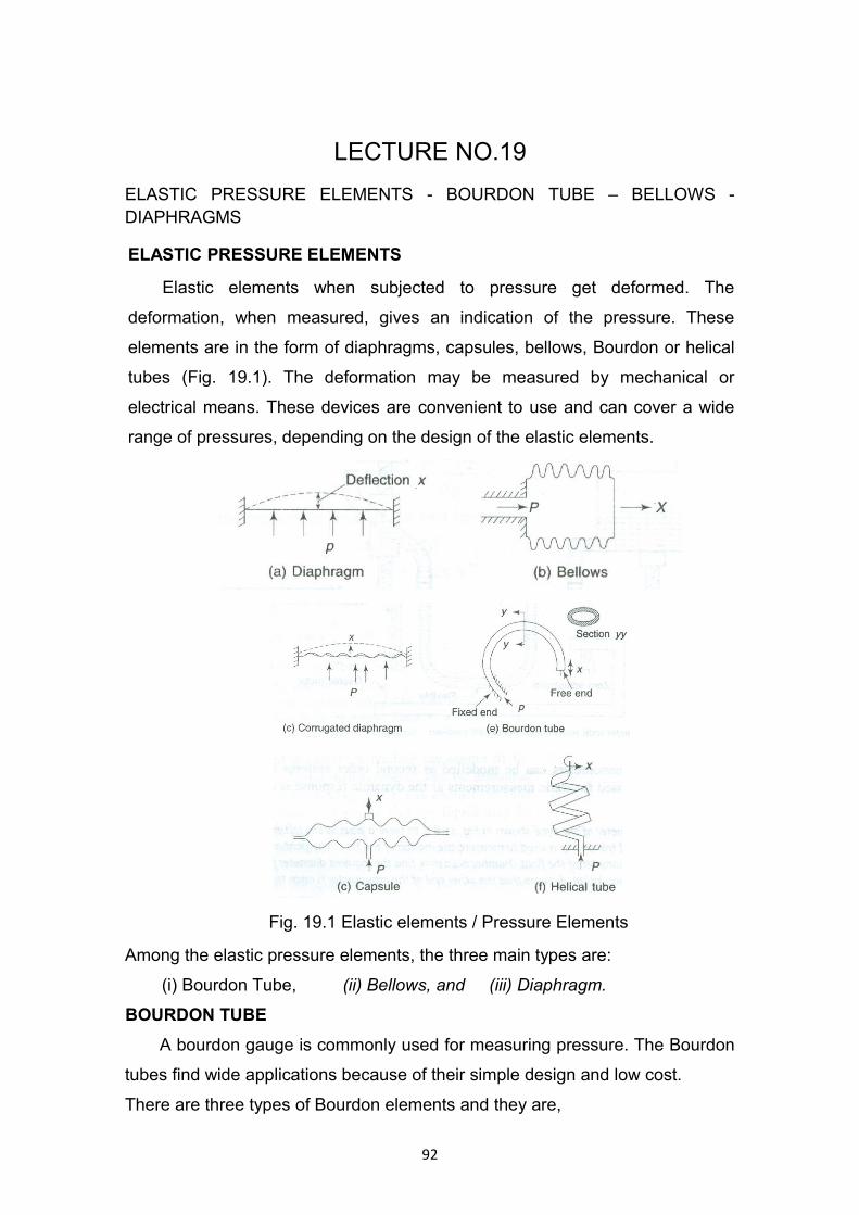
LECTURE NO.19

ELASTIC PRESSURE ELEMENTS - BOURDON TUBE – BELLOWS - DIAPHRAGMS

ELASTIC PRESSURE ELEMENTS

Elastic elements when subjected to pressure get deformed. The

deformation, when measured, gives an indication of the pressure. These

elements are in the form of diaphragms, capsules, bellows, Bourdon or helical

tubes (Fig. 19.1). The deformation may be measured by mechanical or

electrical means. These devices are convenient to use and can cover a wide

range of pressures, depending on the design of the elastic elements.

Fig. 19.1 Elastic elements / Pressure Elements

Among the elastic pressure elements, the three main types are:

(i) Bourdon Tube, (ii) Bellows, and (iii) Diaphragm.

BOURDON TUBE

A bourdon gauge is commonly used for measuring pressure. The Bourdon

tubes find wide applications because of their simple design and low cost.

There are three types of Bourdon elements and they are,

92

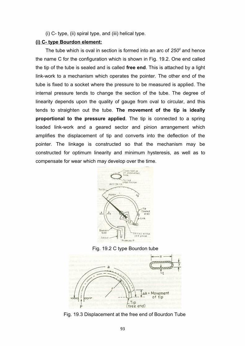
(i) C- type, (ii) spiral type, and (iii) helical type.

(i) C- type Bourdon element:

The tube which is oval in section is formed into an arc of 2500 and hence

the name C for the configuration which is shown in Fig. 19.2. One end called

the tip of the tube is sealed and is called free end. This is attached by a light

link-work to a mechanism which operates the pointer. The other end of the

tube is fixed to a socket where the pressure to be measured is applied. The

internal pressure tends to change the section of the tube. The degree of

linearity depends upon the quality of gauge from oval to circular, and this

tends to straighten out the tube. The movement of the tip is ideally

proportional to the pressure applied. The tip is connected to a spring

loaded link-work and a geared sector and pinion arrangement which

amplifies the displacement of tip and converts into the deflection of the

pointer. The linkage is constructed so that the mechanism may be

constructed for optimum linearity and minimum hysteresis, as well as to

compensate for wear which may develop over the time.

Fig. 19.2 C type Bourdon tube

Fig. 19.3 Displacement at the free end of Bourdon Tube

93

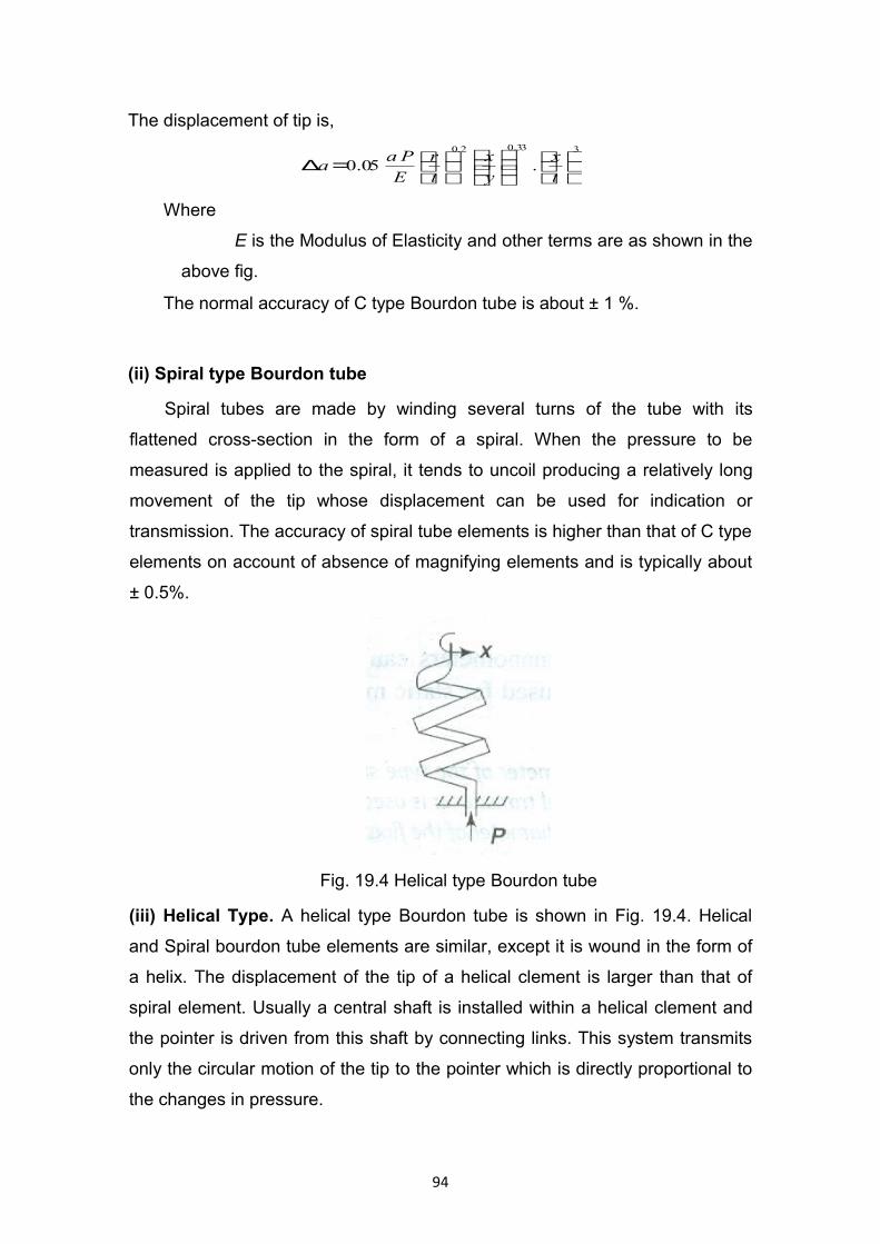
The displacement of tip is,

333.02.0

.05.0

=∆

t

x

y

x

t

r

E

Paa

Where

E is the Modulus of Elasticity and other terms are as shown in the

above fig.

The normal accuracy of C type Bourdon tube is about ± 1 %.

(ii) Spiral type Bourdon tube

Spiral tubes are made by winding several turns of the tube with its

flattened cross-section in the form of a spiral. When the pressure to be

measured is applied to the spiral, it tends to uncoil producing a relatively long

movement of the tip whose displacement can be used for indication or

transmission. The accuracy of spiral tube elements is higher than that of C type

elements on account of absence of magnifying elements and is typically about

± 0.5%.

Fig. 19.4 Helical type Bourdon tube

(iii) Helical Type. A helical type Bourdon tube is shown in Fig. 19.4. Helical

and Spiral bourdon tube elements are similar, except it is wound in the form of

a helix. The displacement of the tip of a helical clement is larger than that of

spiral element. Usually a central shaft is installed within a helical clement and

the pointer is driven from this shaft by connecting links. This system transmits

only the circular motion of the tip to the pointer which is directly proportional to

the changes in pressure.

94

The advantages of helix elements include its stability in fluctuating

pressure applications, and its adaptability for high pressure service. The

number of coils employed in helix elements depends upon the pressure to be

measured. Helix type of pressure elements use as few as three coils while

elements used for measurement for high pressures may have as many as 16

coils or even more. The accuracies obtainable from helical elements may vary

from ± 0.5 % to ± 1 %.

Materials used for constructing Bourdon Tubes

Bourdon tubes are made up of different materials which include brass,

alloy steel, stainless steel, bronze, phosphor bronze, beryllium, copper, and

monel.

Phosphor bronze is used in low pressure applications where the

atmosphere is non-corrosive while in applications where corrosion and / or high

pressure is a problem, stainless steel or Monel are used.

Pressure gauges using bourdon tube elements are made with ranges from

760 mm of mercury to 700 M Pa or higher for special applications with the

minimum span being about 70 kPa.

Bellows

A metallic bellows consists of a series of circular parts, resembling the

folds shown in Fig.19.5. These parts are formed or joined in such a manner

that they are expanded or contracted axially by changes in pressure.

The metals used in the construction of bellows must be

thin enough to be flexible,

ductile enough for reasonably easy fabrication, and

have a high resistance to fatigue failure.

Materials commonly used are brass, bronze, beryllium copper, alloys of

nickel and copper, steel and monel.

95

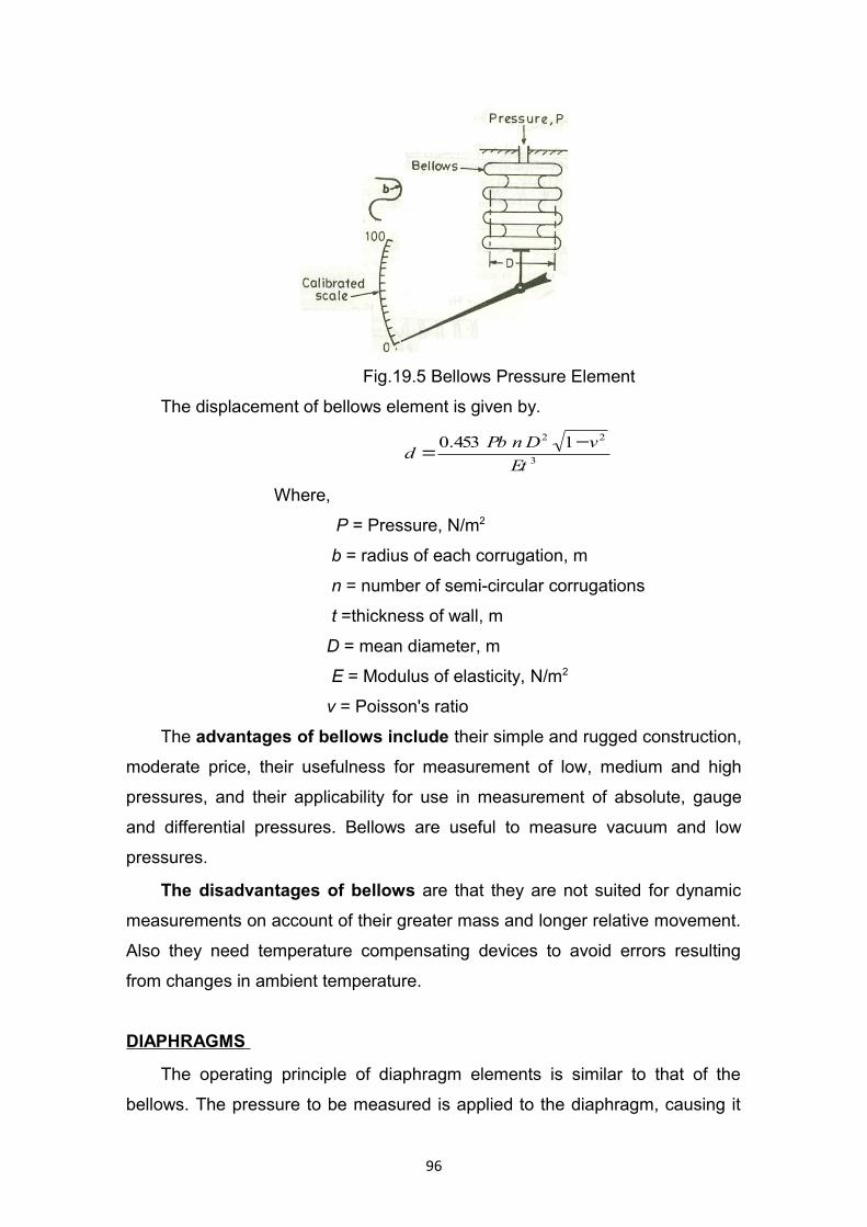
Fig.19.5 Bellows Pressure Element

The displacement of bellows element is given by.

3

22 1453.0

Et

vDnPbd

−=

Where,

P = Pressure, N/m2

b = radius of each corrugation, m

n = number of semi-circular corrugations

t =thickness of wall, m

D = mean diameter, m

E = Modulus of elasticity, N/m2

v = Poisson's ratio

The advantages of bellows include their simple and rugged construction,

moderate price, their usefulness for measurement of low, medium and high

pressures, and their applicability for use in measurement of absolute, gauge

and differential pressures. Bellows are useful to measure vacuum and low

pressures.

The disadvantages of bellows are that they are not suited for dynamic

measurements on account of their greater mass and longer relative movement.

Also they need temperature compensating devices to avoid errors resulting

from changes in ambient temperature.

DIAPHRAGMS

The operating principle of diaphragm elements is similar to that of the

bellows. The pressure to be measured is applied to the diaphragm, causing it

96

to deflect, the deflection being proportional to the applied pressure. The

movement of the diaphragm depends on its thickness and diameter.

The diaphragm element is essentially a flexible disc which may be either

flat or corrugated as shown in Fig. 19.6.

Fig. 19.6 Single Diaphragm elements

For the arrangement of a flat diaphragm shown in Fig. 19.7 the maximum

deflection, dm and the deflection at any radius, dr , are given by following

expressions:

)1(16

3 243

vREt

Pdm −=

and 2223

2

)(16

)1(3rR

Et

vPd r −−=

Fig.19.7 Deflection of flat diaphragm.

In some cases, a diaphragm element may consist of a single disc, while in

others, two diaphragms are bonded together at their circumference by

soldering or pressure welding to form a capsule. A diaphragm element may

consist of one capsule or two or more capsules connected together with each

capsule deflecting on the application of pressure. The total deflection is the

sum of the deflections of individual capsules. Fig. 19.8 shows a diaphragm

element consisting of three capsules. In this assembly, the individual capsule is

97

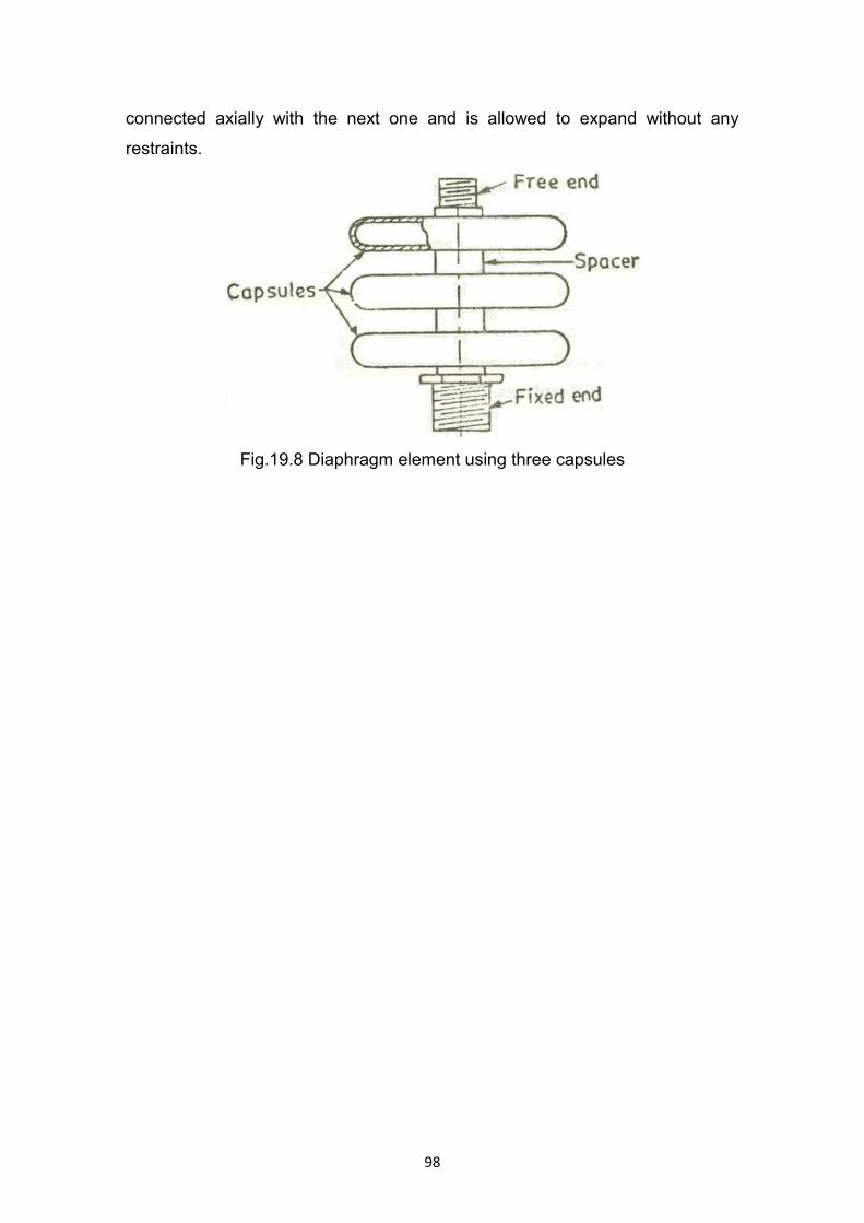
connected axially with the next one and is allowed to expand without any

restraints.

Fig.19.8 Diaphragm element using three capsules

98

LECTURE NO.20

TYPES OF FLUID FLOW: STEADY FLOW AND UNSTEADY FLOW-

UNIFORM FLOW AND NON-UNIFORM FLOW - ONE-DIMENSIONAL FLOW,

TWO DIMENSIONAL FLOW AND THREE DIMENSIONAL FLOW-

ROTATIONAL FLOW AND IRROTATIONAL FLOW - LAMINAR FLOW AND

TURBULENT FLOW.

TYPES OF FLUID FLOW

Fluid flows are classified in several ways as indicated below:

I. Steady flow and Unsteady flow.

II. Uniform flow and Non-uniform flow.

III. One-dimensional flow, two dimensional flow and three dimensional flow.

IV. Rotational flow and Irrotational flow

V. Laminar flow and Turbulent flow.

Steady Flow

Fluid flow is said to be steady if at any point in the flowing fluid various

characteristics such as velocity, pressure, density, temperature etc., which

describe the behavior of the fluid in motion, do not change with time. The

various characteristics of the fluid in motion are independent of time.

However, these characteristics may be different at different points in the

flowing fluid.

Thus the steady flow is expressed mathematically by the following

expression at any point in the flowing fluid.

0=

∂∂t

u; 0=

∂∂t

p; 0=

∂∂t

ρ; 0=

∂∂t

T

Unsteady Flow

Fluid flow is said to be unsteady if at any point in the flowing fluid any

one or all the characteristics which describe the behaviour of the fluid in motion

change with time. Thus a flow of fluid is unsteady, if at any point in the flowing

fluid

99

0≠

∂∂t

V; 0≠

∂∂t

p etc.

Steady flow is simpler to analyze than unsteady flow. Most of the

practical problems of engineering involve only steady flow conditions.

Uniform Flow

When the velocity of flow of fluid does not change, both in magnitude

and direction, from point to point in the flowing fluid, for any given instant of

time, the flow is said to be uniform. In the mathematical form a uniform flow

may therefore be expressed as

0=

∂∂s

V t= constant

where time is held constant and s represents any direction of displacement of

the fluid elements. The above expression states that there is no change in the

velocity vector in any direction throughout the flowing fluid at any instant of

time. For example flow of liquids under pressure through long pipe lines of

constant diameter is uniform flow.

Non-uniform Flow

If the velocity of flow of fluid changes from point to point in the flowing

fluid at any instant, the flow is said to be non-uniform. In the mathematical form

a non-uniform flow may be expressed as

0≠

∂∂s

V

For example, flow of liquids under pressure through long pipelines of

varying diameters is non-uniform flow.

All these types of flows can exist independent of each other so that any

of the four types of combinations of flows is possible, viz., (a) steady-uniform

flow; (b) steady-non-uniform flow; (c) unsteady uniform flow; and (d) unsteady-

non-uniform flow. Examples of these combinations of flows are:

100

flow of liquid through a long pipe of constant diameter at a constant rate

is steady uniform flow;

flow of liquid through a long pipe line of constant diameter, at either

increasing or decreasing rate is unsteady-uniform flow;

flow of liquid through a tapering pipe at a constant rate is steady-non-

uniform flow and

flow through a tapering pipe at either increasing or decreasing rate is

unsteady-non-uniform flow.

One-dimensional, Two-dimensional and Three-dimensional Flows

The various characteristics of flowing fluid such as velocity, pressure,

density, temperature etc, are in general the functions of space and time i.e.,

these may vary with the coordinates of any point x, y and z and time t. Such a

flow is known as a three-dimensional flow. If any of these characteristics of

flowing fluid does not vary with respect to time, then it will be a steady three-

dimensional flow.

When the various characteristics of flowing fluid are the functions of only

any two of the three coordinate directions, and time t, i.e., these may not vary in

anyone of the directions, then the flow is known as two-dimensional flow. For

example, if the characteristics of flowing fluid do not vary in the coordinate

direction Z, then it will be a two-dimensional flow having flow conditions

identical in the various planes perpendicular to the Z-axis.

When the various characteristics of flowing fluid are the functions of only

one of the three coordinate directions and time t, i.e., these may vary only in

one direction, then the flow is known as one dimensional flow. Similarly, it will

be a steady one dimensional flow if the characteristics of flowing fluid do not

vary with respect to time. Considering one of the characteristics of flowing

mass of fluid, say velocity of flow V, the following expressions may be written

which clearly exhibit the difference between these three types of flows:

Types of Flow Unsteady Steady

Three dimensional ( )tzyxfV ,,,= ( )zyxfV ,,=

101

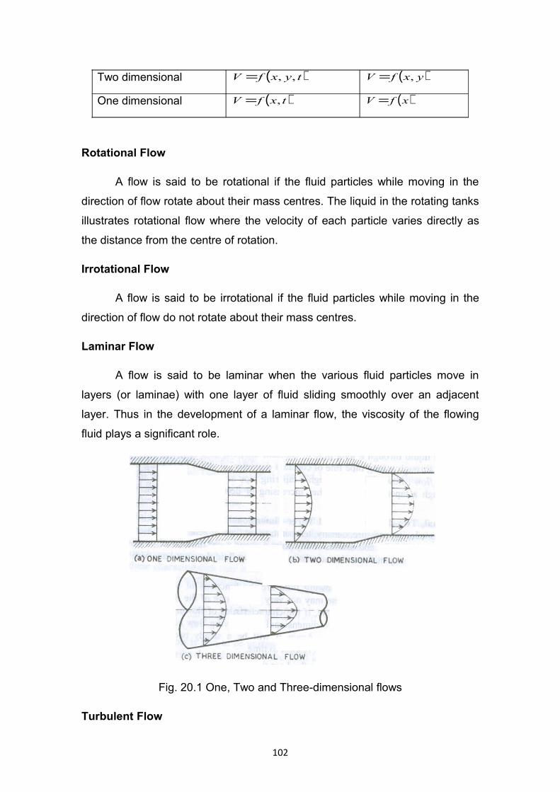
Two dimensional ( )tyxfV ,,= ( )yxfV ,=

One dimensional ( )txfV ,= ( )xfV =

Rotational Flow

A flow is said to be rotational if the fluid particles while moving in the

direction of flow rotate about their mass centres. The liquid in the rotating tanks

illustrates rotational flow where the velocity of each particle varies directly as

the distance from the centre of rotation.

Irrotational Flow

A flow is said to be irrotational if the fluid particles while moving in the

direction of flow do not rotate about their mass centres.

Laminar Flow

A flow is said to be laminar when the various fluid particles move in

layers (or laminae) with one layer of fluid sliding smoothly over an adjacent

layer. Thus in the development of a laminar flow, the viscosity of the flowing

fluid plays a significant role.

Fig. 20.1 One, Two and Three-dimensional flows

Turbulent Flow

102

A fluid motion is said to be turbulent when the fluid particles move in an

entirely haphazard or disorderly manner that results in a rapid and continuous

mixing of the fluid leading to momentum transfer as flow occurs. In such a flow

eddies or vortices of different sizes and shapes are present which move over

large distances. This eddies and their random movement give rise to

fluctuations in the velocity and pressure at any point in the flow field, which are

necessarily the functions of time.

103

LECTURE NO.21

FLOW MEASUREMENT: INTRODUCTION - PRIMARY OR QUANTITY

METERS - POSITIVE-DISPLACEMENT METERS - SECONDARY OR RATE

METERS - VARIABLE HEAD METERS

FLOW MEASUREMENT: Introduction

Flow measurements are essential in many applications such as

transportation of solids as slurries, compressed natural gas in pipelines, water

and gas supply systems to domestic consumers, irrigation systems and a

number of industrial process control systems. The types of flows encountered

in the measurements may be any one or combination of the following types:

• clean or dirty/opaque,

• wet or dry,

• hazardous/corrosive or safe,

• single-phase, two-phase or multiphase,

• laminar or transitional or turbulent,

• pressure may vary from vacuums to high pressures of many

atmospheres,

• temperature may vary from cryogenic levels to hundreds of

centigrade,

• flow rate may be of miniscule type, i.e., few drops per minute or

massive type involving thousands of litres per minute.

The selection of a particular flow-measuring equipment depends

primarily on the nature of the metered fluid and the demands of the associated

plant. Many industrial flow meters have to work with fluids which may be

corrosive in nature or may contain foreign matters, but the equipment may be

relatively large and of fixed type. Additionally, the other factors that govern the

choice of a particular flow metering device are the various performance

parameters like range, accuracy, repeatability, linearity, dynamic response,

type of output like analog / digital, etc. Further, another requirement may be to

indicate or record the rate of flow, total flow or may be both these quantities.

104

Flow measuring devices generally fall into one of the two categories,

namely, primary devices or quantity meters and secondary devices known as

rate meters. The distinction between the two is based on the character of the

sensing element that interacts with the fluid flow. Quantity measurements, by

mass or volume, are usually accomplished by counting successive isolated

portions, whereas rate measurements are inferred from effects of flow rates on

pressure, force, heat transfer, flow area, etc. The quantity meters are generally

used for the calibration of rate meters.

PRIMARY OR QUANTITY METERS

Quantity or total flow measurement signifies the amount of fluid in terms

of mass or volume that flows past a given point in a definite period of time. In

other words, in this technique, the time required to collect a particular amount

of fluid is determined accurately and then the average flow rate can be

evaluated.

The flow meter calibration procedures using the quantity measurements

fall into the following two categories.

1. Voumetric Method

2. Gravimetric Method

Volumetric Method

In this technique, the fluid flowing in the flow meter which is being

calibrated is diverted into a tank of known volume. When the tank is completely

filled, then this known volume is compared with the integrated, volumetric

quantity registered by the flow meter under test.

Gravimetric Method

In this technique also, the fluid flowing in the flow meter, which is being

calibrated, is diverted into a vessel which can be weighed either continuously or

in the vessel after a pre-determined time. The weight of the liquid collected is

compared with the gravimetric quantity registered by the flow meter under test.

105

POSITIVE-DISPLACEMENT METERS

The term positive displacement meter is applied to a flow measuring

device so designed that the metered fluid is repeatedly filled and emptied from

a space of known volume. The principle of this measurement is that the

liquid flows through a meter and moves the measuring element that seals

the measuring chamber into a series of measuring compartments each

holding a definite volume. Each element is successively filled from the flow at

the inlet and emptied at the outlet of the meter. In other words, it is said that

positive-displacement meters chop the flow into ‘pieces' of known size and then

count the number of ‘pieces’.

Positive-displacement meters are widely used in low flow rate metering

applications where high accuracy and repeatability under steady flow

conditions are required. Further, they are easy to install and maintain and have

moderate cost. These types of meters are generally used by the water and oil

undertakings for accounting purposes. However, since there are moving parts

in these devices, the wear of the components may alter the accuracy.

Therefore, these instruments need calibration/adjustment over an interval of

time. Another limitation of such meters is their suitability to clean fluids only.

Further, these devices are generally flow totalizers and do not give

instantaneous rate of flow.

SECONDARY OR RATE METERS

The secondary or rate meters are also termed as inferential type of flow

measuring devices. This is because of the fact that they do not measure the

flow directly but instead measure another physical quantity which is related to

the flow. These devices fall into two categories, namely, the flow rate meters

and the velocity meters.

The transduction principle of some typical flow rate meters is as follows:

(i) Variable head meters: These are also termed as obstruction type of meters

in which the obstruction to the flow consists of an engineered constriction in the

metered fluid which causes a reduction in the flow pressure.

106

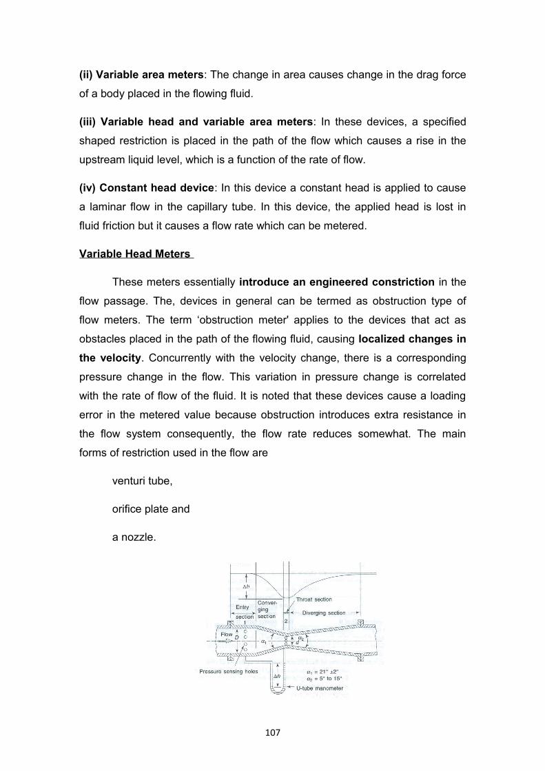
(ii) Variable area meters: The change in area causes change in the drag force

of a body placed in the flowing fluid.

(iii) Variable head and variable area meters: In these devices, a specified

shaped restriction is placed in the path of the flow which causes a rise in the

upstream liquid level, which is a function of the rate of flow.

(iv) Constant head device: In this device a constant head is applied to cause

a laminar flow in the capillary tube. In this device, the applied head is lost in

fluid friction but it causes a flow rate which can be metered.

Variable Head Meters

These meters essentially introduce an engineered constriction in the

flow passage. The, devices in general can be termed as obstruction type of

flow meters. The term ‘obstruction meter' applies to the devices that act as

obstacles placed in the path of the flowing fluid, causing localized changes in

the velocity. Concurrently with the velocity change, there is a corresponding

pressure change in the flow. This variation in pressure change is correlated

with the rate of flow of the fluid. It is noted that these devices cause a loading

error in the metered value because obstruction introduces extra resistance in

the flow system consequently, the flow rate reduces somewhat. The main

forms of restriction used in the flow are

venturi tube,

orifice plate and

a nozzle.

107

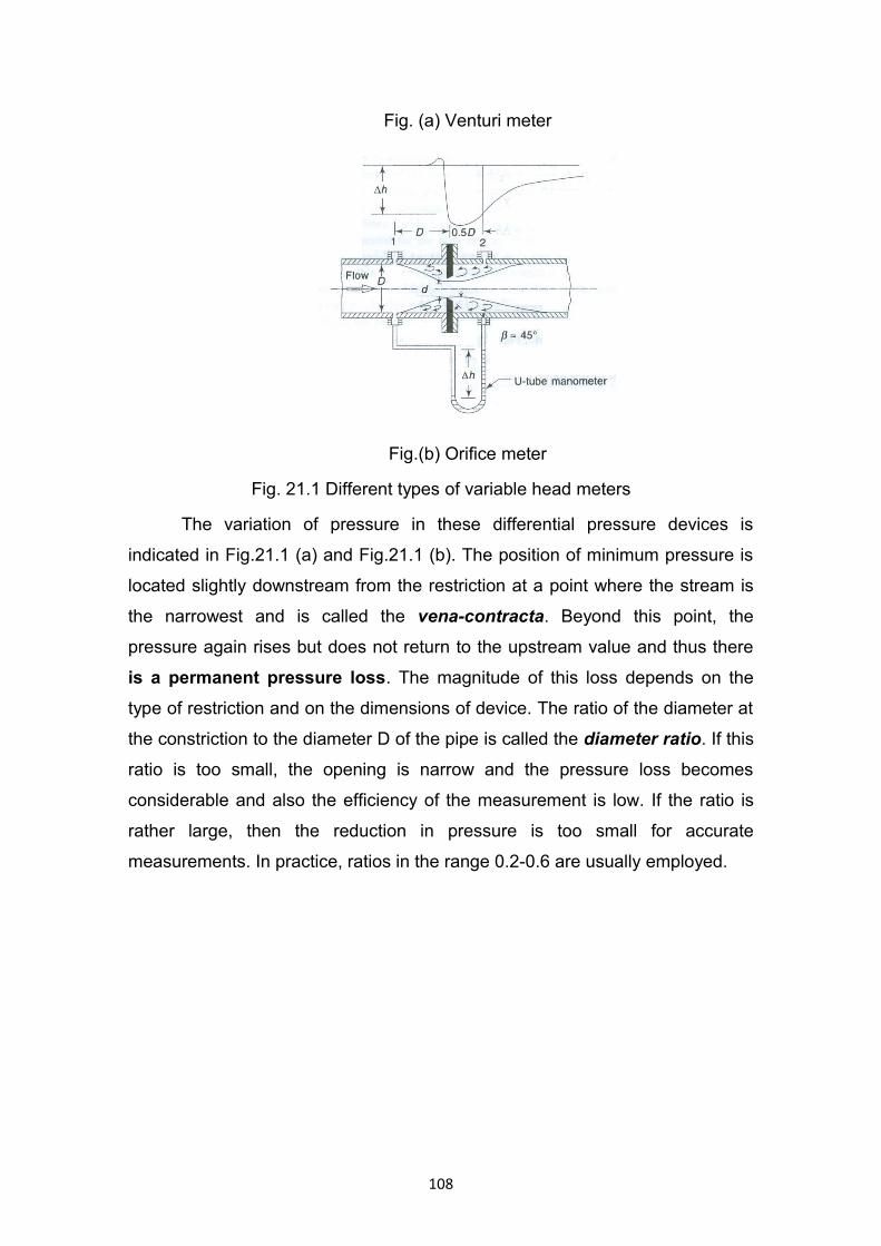
Fig. (a) Venturi meter

Fig.(b) Orifice meter

Fig. 21.1 Different types of variable head meters

The variation of pressure in these differential pressure devices is

indicated in Fig.21.1 (a) and Fig.21.1 (b). The position of minimum pressure is

located slightly downstream from the restriction at a point where the stream is

the narrowest and is called the vena-contracta. Beyond this point, the

pressure again rises but does not return to the upstream value and thus there

is a permanent pressure loss. The magnitude of this loss depends on the

type of restriction and on the dimensions of device. The ratio of the diameter at

the constriction to the diameter D of the pipe is called the diameter ratio. If this

ratio is too small, the opening is narrow and the pressure loss becomes

considerable and also the efficiency of the measurement is low. If the ratio is

rather large, then the reduction in pressure is too small for accurate

measurements. In practice, ratios in the range 0.2-0.6 are usually employed.

108

LECTURE NO.22

THE GENERAL EXPRESSION FOR THE RATE OF FLOW- CONSTRUCTION

OF VENTURI METER

The general expression for the rate of flow in these devices can be

derived as follows:

Say, the pressure, velocity and area of fluid stream at point 1, upstream

of obstruction are 111, AandVp and at point 2 just downstream of the

obstruction are 222 , AandVp . Further, we assume the flow to be

incompressible, i.e., its density does not vary in the flow field.

Applying the continuity equation in the flow we get

Rate of discharge 2211 VAVAQ == ------

(22.1)

Applying Bernoulli's equation (assuming the flow to be ideal) we get,

22

22

2

21

1

VP

VP

ρρ +=+

(22.2)

The differential pressure head h∆ is given by

hg

pp ∆=−ρ

21

(22.3)

Eliminating V1 and V2 from Eqs. (22.1) and (22.2) and substituting the

value of h∆ from eq. (3) we get the ideal rate of discharge as

hgAA

AAQideal ∆

−= 2.

22

21

21

(22.4)

In actual practice, the actual rate of fluid flow is always less than Qideal as

given by eq.(22.4), because of the losses in the fluid flow due to friction and

109

eddying motions. To account for this discrepancy, we define the term

coefficient of discharge Cd as

ideal

actuald Q

QC = (22.5)

Thus, we can write the actual rate of fluid flow as

hgAA

AACQ dactual ∆

−= 2.

22

21

21(22.6)

Equation (22.6) can be rewritten in the simplified from as

21)( hKCQ dactual ∆=

(22.7)

Where K is the constant of low obstruction device and

gAA

AAK 2.

22

21

21

−=

where dC is the coefficient of discharge which depends on the type of flow,

obstruction type configuration and also on the Reynolds number of the flow.

Reynolds number = µρVD

The venturimeter offers the best accuracy, least head loss as compared

to the orifice meter. Because of the smooth surface, it is not much affected by

the wear and abrasion from dirty fluids. Further, due to low value of losses, the

coefficient of discharge is high and approaches unity under favourable

conditions. However, it is expensive and occupies substantial space.

An orifice meter consists of thin orifice plate which may be clamped

between pipe flanges. Since its geometry is simple, it is low in cost, easy to

install or replace and takes almost no space. However, it suffers from a head

loss which is of the order of 30-40%. Also, it is susceptible to inaccuracies

resulting from erosion, corrosion, clogging, etc. due to flow of dirty fluids.

110

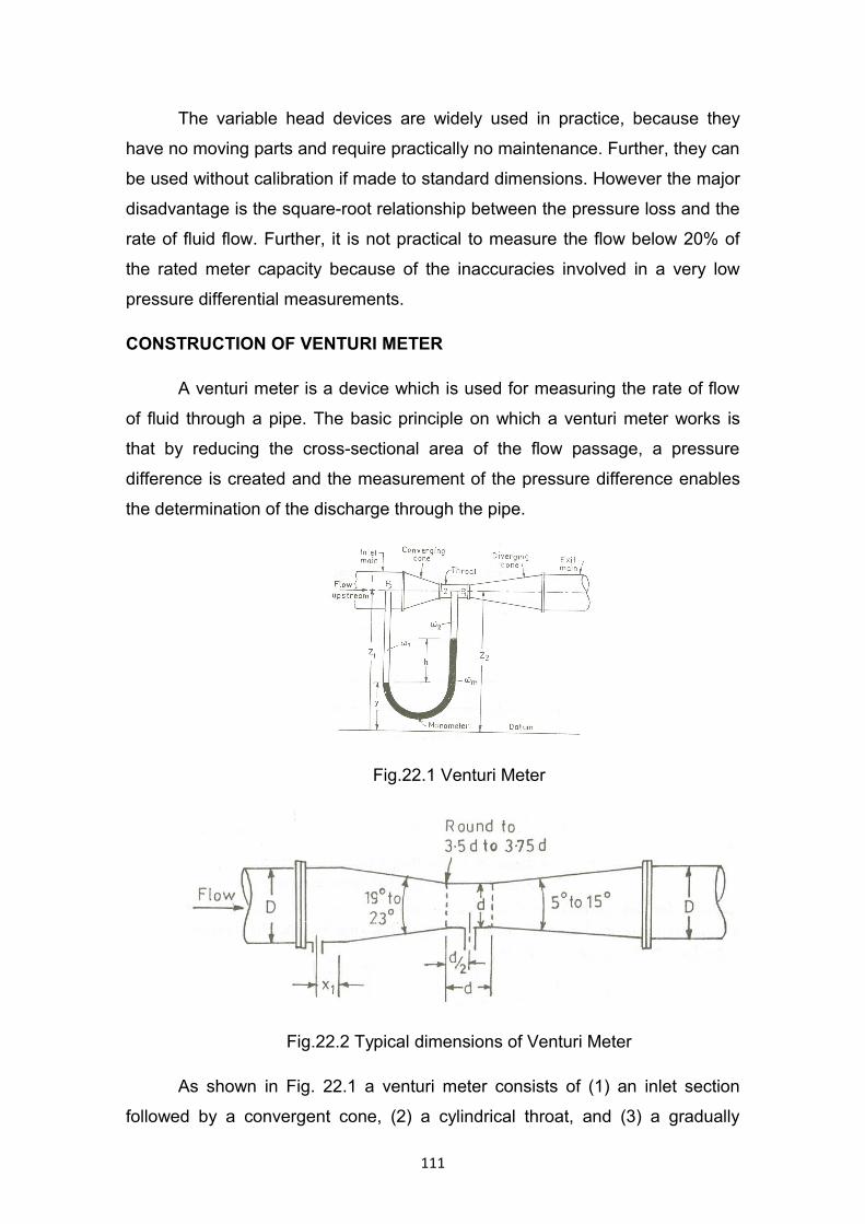
The variable head devices are widely used in practice, because they

have no moving parts and require practically no maintenance. Further, they can

be used without calibration if made to standard dimensions. However the major

disadvantage is the square-root relationship between the pressure loss and the

rate of fluid flow. Further, it is not practical to measure the flow below 20% of

the rated meter capacity because of the inaccuracies involved in a very low

pressure differential measurements.

CONSTRUCTION OF VENTURI METER

A venturi meter is a device which is used for measuring the rate of flow

of fluid through a pipe. The basic principle on which a venturi meter works is

that by reducing the cross-sectional area of the flow passage, a pressure

difference is created and the measurement of the pressure difference enables

the determination of the discharge through the pipe.

Fig.22.1 Venturi Meter

Fig.22.2 Typical dimensions of Venturi Meter

As shown in Fig. 22.1 a venturi meter consists of (1) an inlet section

followed by a convergent cone, (2) a cylindrical throat, and (3) a gradually

111

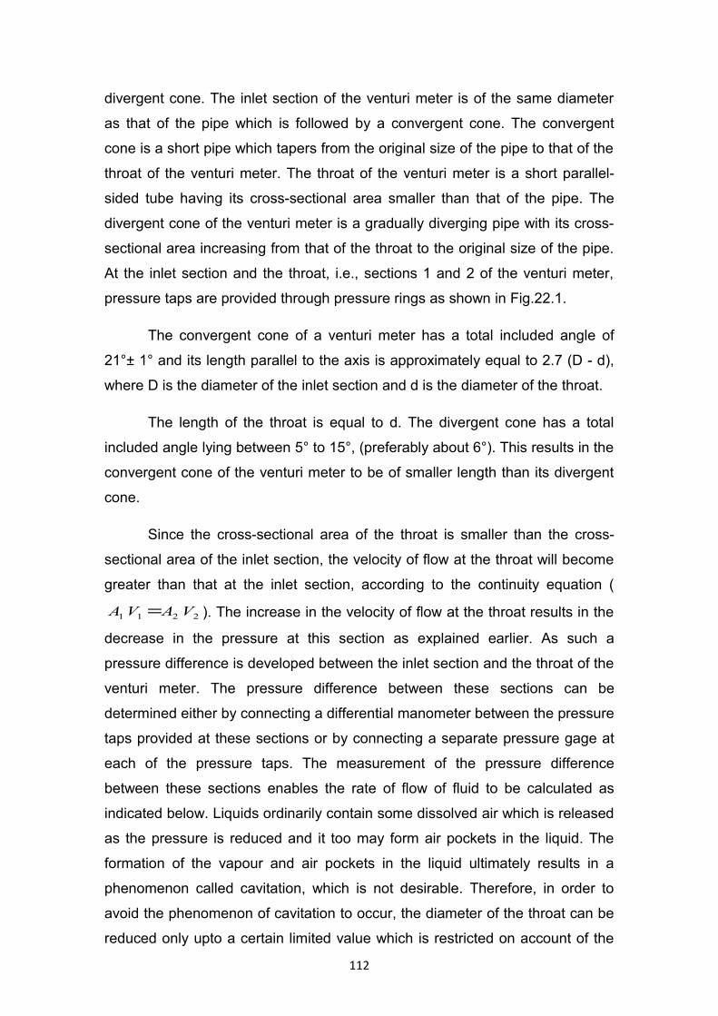
divergent cone. The inlet section of the venturi meter is of the same diameter

as that of the pipe which is followed by a convergent cone. The convergent

cone is a short pipe which tapers from the original size of the pipe to that of the

throat of the venturi meter. The throat of the venturi meter is a short parallel-

sided tube having its cross-sectional area smaller than that of the pipe. The

divergent cone of the venturi meter is a gradually diverging pipe with its cross-

sectional area increasing from that of the throat to the original size of the pipe.

At the inlet section and the throat, i.e., sections 1 and 2 of the venturi meter,

pressure taps are provided through pressure rings as shown in Fig.22.1.

The convergent cone of a venturi meter has a total included angle of

21°± 1° and its length parallel to the axis is approximately equal to 2.7 (D - d),

where D is the diameter of the inlet section and d is the diameter of the throat.

The length of the throat is equal to d. The divergent cone has a total

included angle lying between 5° to 15°, (preferably about 6°). This results in the

convergent cone of the venturi meter to be of smaller length than its divergent

cone.

Since the cross-sectional area of the throat is smaller than the cross-

sectional area of the inlet section, the velocity of flow at the throat will become

greater than that at the inlet section, according to the continuity equation (

2211 VAVA = ). The increase in the velocity of flow at the throat results in the

decrease in the pressure at this section as explained earlier. As such a

pressure difference is developed between the inlet section and the throat of the

venturi meter. The pressure difference between these sections can be

determined either by connecting a differential manometer between the pressure

taps provided at these sections or by connecting a separate pressure gage at

each of the pressure taps. The measurement of the pressure difference

between these sections enables the rate of flow of fluid to be calculated as

indicated below. Liquids ordinarily contain some dissolved air which is released

as the pressure is reduced and it too may form air pockets in the liquid. The

formation of the vapour and air pockets in the liquid ultimately results in a

phenomenon called cavitation, which is not desirable. Therefore, in order to

avoid the phenomenon of cavitation to occur, the diameter of the throat can be

reduced only upto a certain limited value which is restricted on account of the

112

above noted factors. In general, the diameter of the throat may vary from 3

1 to

4

3 of the pipe diameter and more commonly the diameter of the throat is kept

equal to 1/2 of the pipe diameter.

113

LECTURE NO.23

CONSTRUCTION OF ORIFICE METER

An orifice meter is another simple device used for measuring the

discharge through pipes. Orifice meter also works on the same principle as that

of venturi meter i.e., by reducing the cross-sectional area of the flow passage a

pressure difference between the two sections is developed and the

measurement of the pressure difference enables the determination of the

discharge through the pipe. However, an orifice meter is a cheaper

arrangement for discharge measurement through pipes and its installation

requires a smaller length as compared with venturi meter. As such where the

space is limited, the orifice meter may be used for the measurement of

discharge through pipes.

An orifice meter consists of a flat circular plate with a circular hole called

orifice, which is concentric with the pipe axis. The thickness of the plate t is less

than or equal to 0.05 times the diameter of the pipe. From the upstream face of

the plate the edge of the orifice is made flat for a thickness t1 less then or equal

to 0.02 times the diameter of the pipe and for the remaining thickness of the

plate it is bevelled with the bevel angle lying between 30° to 45° (preferably

45°).

Fig. 23.1 Orifice meter

114

Fig.23.2 Concentric orifice plate with 45 ° bevelled edges

Fig.23.3 Eccentric orifice plate

Fig.23.4 Segmental orifice plate

115

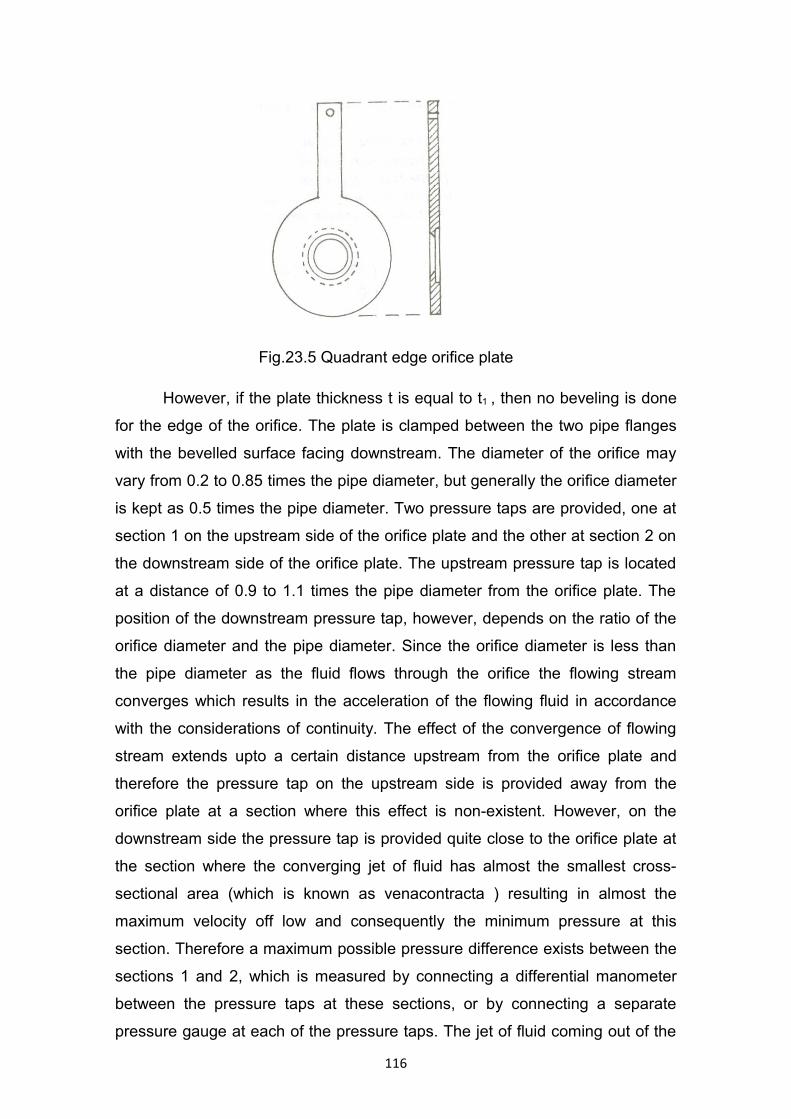
Fig.23.5 Quadrant edge orifice plate

However, if the plate thickness t is equal to t1 , then no beveling is done

for the edge of the orifice. The plate is clamped between the two pipe flanges

with the bevelled surface facing downstream. The diameter of the orifice may

vary from 0.2 to 0.85 times the pipe diameter, but generally the orifice diameter

is kept as 0.5 times the pipe diameter. Two pressure taps are provided, one at

section 1 on the upstream side of the orifice plate and the other at section 2 on

the downstream side of the orifice plate. The upstream pressure tap is located

at a distance of 0.9 to 1.1 times the pipe diameter from the orifice plate. The

position of the downstream pressure tap, however, depends on the ratio of the

orifice diameter and the pipe diameter. Since the orifice diameter is less than

the pipe diameter as the fluid flows through the orifice the flowing stream

converges which results in the acceleration of the flowing fluid in accordance

with the considerations of continuity. The effect of the convergence of flowing

stream extends upto a certain distance upstream from the orifice plate and

therefore the pressure tap on the upstream side is provided away from the

orifice plate at a section where this effect is non-existent. However, on the

downstream side the pressure tap is provided quite close to the orifice plate at

the section where the converging jet of fluid has almost the smallest cross-

sectional area (which is known as venacontracta ) resulting in almost the

maximum velocity off low and consequently the minimum pressure at this

section. Therefore a maximum possible pressure difference exists between the

sections 1 and 2, which is measured by connecting a differential manometer

between the pressure taps at these sections, or by connecting a separate

pressure gauge at each of the pressure taps. The jet of fluid coming out of the

116

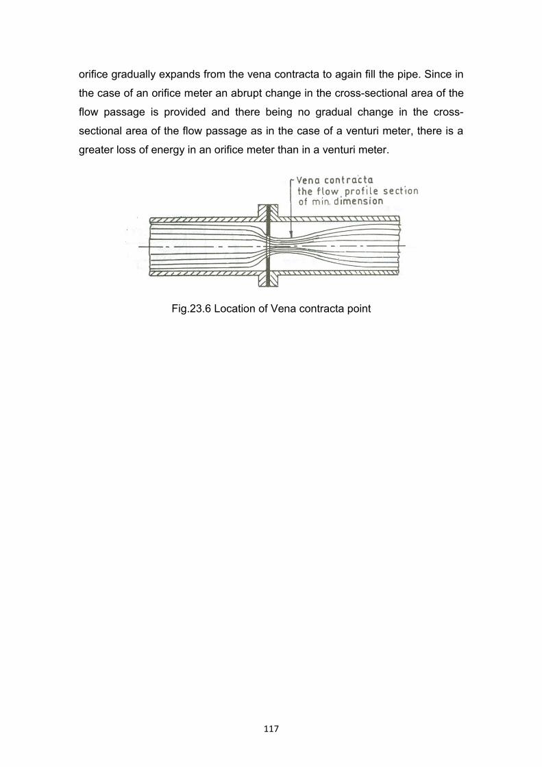
orifice gradually expands from the vena contracta to again fill the pipe. Since in

the case of an orifice meter an abrupt change in the cross-sectional area of the

flow passage is provided and there being no gradual change in the cross-

sectional area of the flow passage as in the case of a venturi meter, there is a

greater loss of energy in an orifice meter than in a venturi meter.

Fig.23.6 Location of Vena contracta point

117

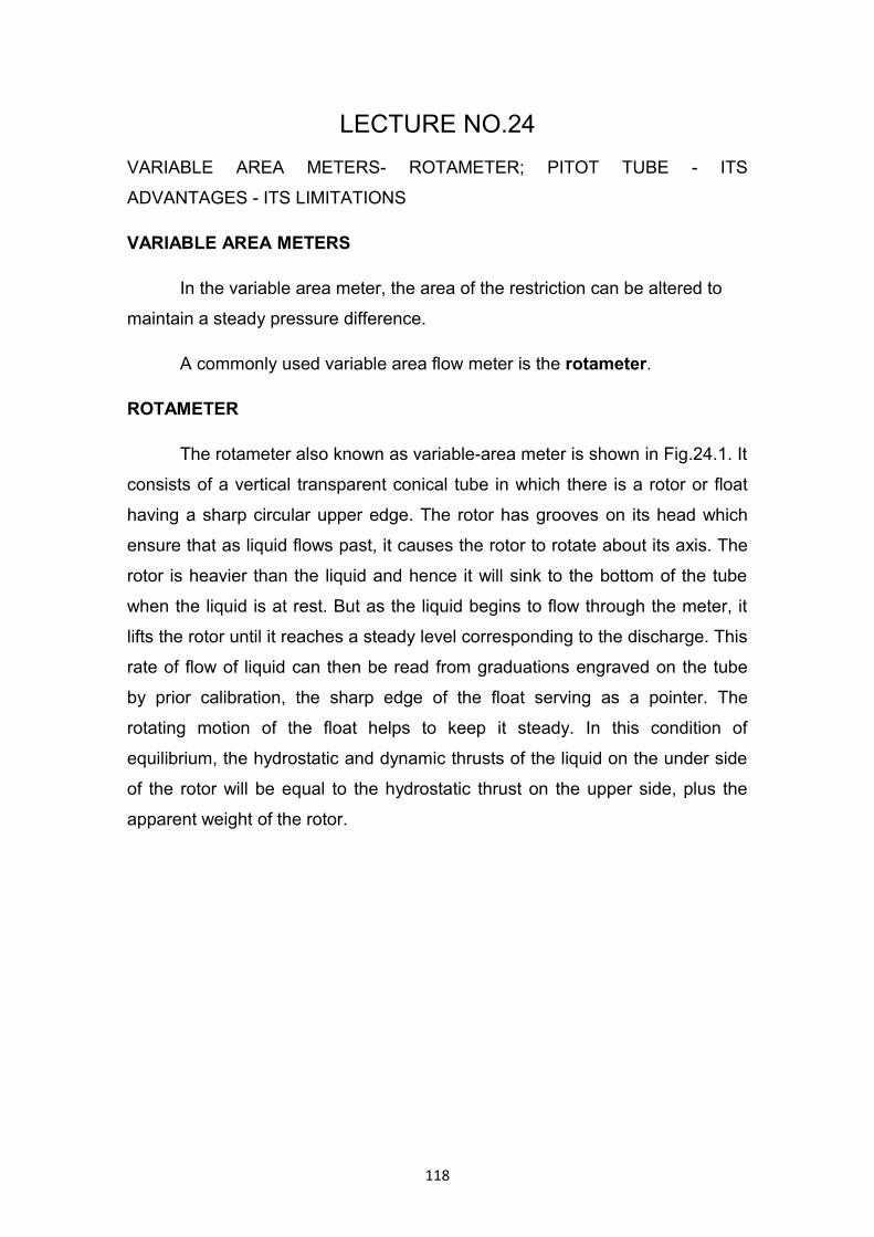
LECTURE NO.24

VARIABLE AREA METERS- ROTAMETER; PITOT TUBE - ITS

ADVANTAGES - ITS LIMITATIONS

VARIABLE AREA METERS

In the variable area meter, the area of the restriction can be altered to

maintain a steady pressure difference.

A commonly used variable area flow meter is the rotameter.

ROTAMETER

The rotameter also known as variable-area meter is shown in Fig.24.1. It

consists of a vertical transparent conical tube in which there is a rotor or float

having a sharp circular upper edge. The rotor has grooves on its head which

ensure that as liquid flows past, it causes the rotor to rotate about its axis. The

rotor is heavier than the liquid and hence it will sink to the bottom of the tube

when the liquid is at rest. But as the liquid begins to flow through the meter, it

lifts the rotor until it reaches a steady level corresponding to the discharge. This

rate of flow of liquid can then be read from graduations engraved on the tube

by prior calibration, the sharp edge of the float serving as a pointer. The

rotating motion of the float helps to keep it steady. In this condition of

equilibrium, the hydrostatic and dynamic thrusts of the liquid on the under side

of the rotor will be equal to the hydrostatic thrust on the upper side, plus the

apparent weight of the rotor.

118

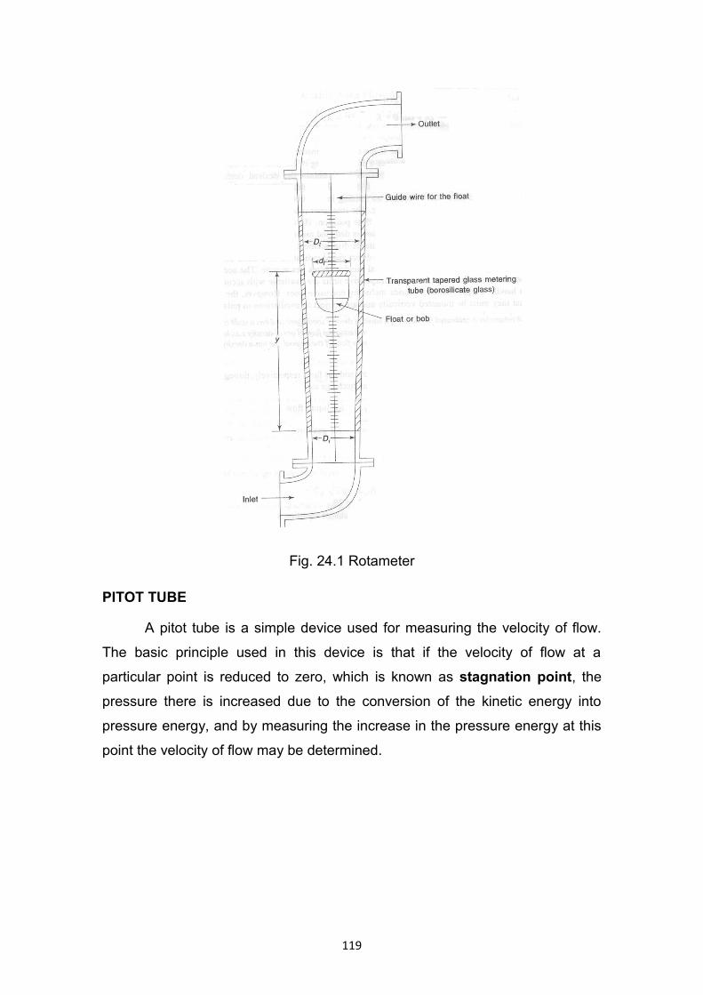
Fig. 24.1 Rotameter

PITOT TUBE

A pitot tube is a simple device used for measuring the velocity of flow.

The basic principle used in this device is that if the velocity of flow at a

particular point is reduced to zero, which is known as stagnation point, the

pressure there is increased due to the conversion of the kinetic energy into

pressure energy, and by measuring the increase in the pressure energy at this

point the velocity of flow may be determined.

119

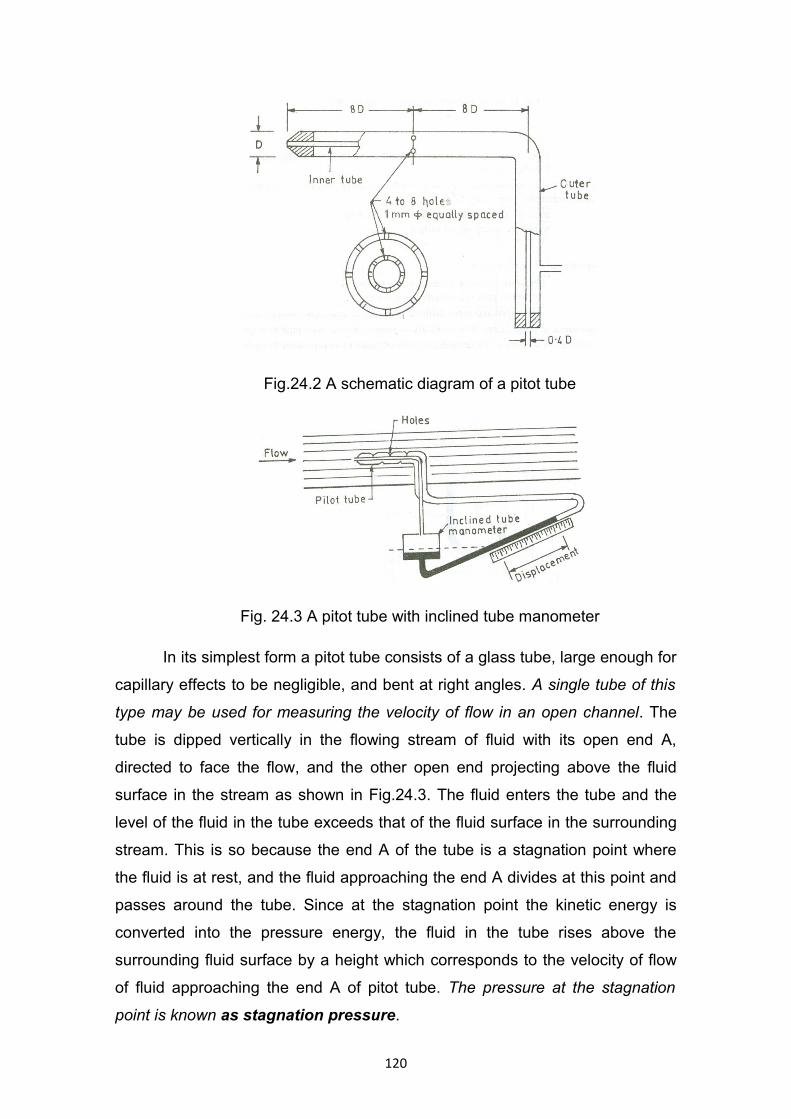
Fig.24.2 A schematic diagram of a pitot tube

Fig. 24.3 A pitot tube with inclined tube manometer

In its simplest form a pitot tube consists of a glass tube, large enough for

capillary effects to be negligible, and bent at right angles. A single tube of this

type may be used for measuring the velocity of flow in an open channel. The

tube is dipped vertically in the flowing stream of fluid with its open end A,

directed to face the flow, and the other open end projecting above the fluid

surface in the stream as shown in Fig.24.3. The fluid enters the tube and the

level of the fluid in the tube exceeds that of the fluid surface in the surrounding

stream. This is so because the end A of the tube is a stagnation point where

the fluid is at rest, and the fluid approaching the end A divides at this point and

passes around the tube. Since at the stagnation point the kinetic energy is

converted into the pressure energy, the fluid in the tube rises above the

surrounding fluid surface by a height which corresponds to the velocity of flow

of fluid approaching the end A of pitot tube. The pressure at the stagnation

point is known as stagnation pressure.

120

Consider a point 1 slightly upstream of end A and lying along the same

horizontal plane in the flowing stream where the velocity of flow is V. Now if the

points 1 and A are at a vertical depth of ho below the free surface of fluid in the

stream and h is the height of the fluid raised in the pitot tube above the free

surface, then applying Bernoulli's equation between the points 1 and A and

neglecting the loss of energy, we get

hhg

Vh o +=+

2

2

0

In the above expression (ho + h), is the stagnation pressure head at

point A, which consists of two parts viz., the static pressure head ho and the

dynamic pressure head h. By simplifying the expression, we get

hg

V =2

2

;

or ghV 2=

Above equation indicates that the dynamic pressure head h is

proportional to the square of the velocity of flow in the stream at the point close

to the end A of the Pitot tube. Thus the velocity of flow at any point in the

flowing stream may be determined by dipping the pitot tube to the required

point and measuring the height h of the fluid raised in the tube above the free

surface. However, the velocity of flow given by equation is somewhat more

than the actual velocity of flow, because in deriving the above equation no loss

of energy has been considered. Moreover, when the flow is highly turbulent the

pitot tube records a value of h which is higher than that corresponding to the

mean velocity of flow in the direction of the tube axis. As such in order to take

into account the errors which may creep in due to the above noted factors the

actual velocity of flow may be obtained by introducing a coefficient C (or Cv)

called pitot tube coefficient, so that the actual velocity of flow is given by

ghCV 2=

A probable value for the coefficient of the pitot tube, C is 0.98. However,

the actual value of the coefficient C for a pitot tube may be determined by

calibration.

121

When a pitot tube is used for measuring the velocity of flow in a pipe or

any other closed conduit then the pitot tube may be inserted. Since a pitot tube

measures the stagnation pressure head (or the total head) at its dipped end,

the static pressure head is also required to be measured at the same section

where the tip of the pitot tube is held, in order to determine the dynamic

pressure head h. For measuring the static pressure head a pressure tap (or a

static orifice) is provided at this section to which a piezometer may be

connected. Alternatively the dynamic pressure head may also be determined

directly by connecting a suitable differential manometer between the pitot tube

and the pressure tap meant for measuring the static pressure.

The pitot tube has the following advantages:

1. It is a simple and low-cost device,

2. It produces no appreciable pressure loss in the flow system,

3. It can be easily inserted through a small hole into the pipe or duct, and

4. It is very useful for checking the mean velocities of the flows in

venturi, nozzle, orifice plate or any other complex flow field.

The limitations of this device are follows:

1. It is not suitable for measuring low velocities, i.e., below 5 m/s,

because of difficulties in the accurate measurement of pressure

differential.

2. It is sensitive to misalignment of the probe with respect to free stream

velocity. Usually an angle of yaw or misalignment up to 5° has little

effect on the velocity values but beyond 20° the error in the velocity

determination is of the order of 2%.

3. It is not suitable for the measurement of highly fluctuating velocities,

i.e., highly turbulent flows.

4. The use of pitot-tube is limited to exploratory studies. It is not

commonly used in industrial applications as numerous pitot tube

122

traverses are required for velocity distribution data which is quite

tedious and time-consuming.

123

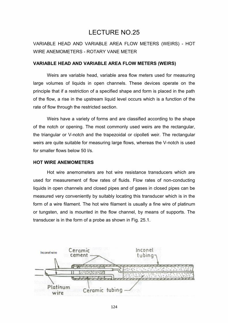
LECTURE NO.25

VARIABLE HEAD AND VARIABLE AREA FLOW METERS (WEIRS) - HOT

WIRE ANEMOMETERS - ROTARY VANE METER

VARIABLE HEAD AND VARIABLE AREA FLOW METERS (WEIRS)

Weirs are variable head, variable area flow meters used for measuring

large volumes of liquids in open channels. These devices operate on the

principle that if a restriction of a specified shape and form is placed in the path

of the flow, a rise in the upstream liquid level occurs which is a function of the

rate of flow through the restricted section.

Weirs have a variety of forms and are classified according to the shape

of the notch or opening. The most commonly used weirs are the rectangular,

the triangular or V-notch and the trapezoidal or cipolleti weir. The rectangular

weirs are quite suitable for measuring large flows, whereas the V-notch is used

for smaller flows below 50 l/s.

HOT WIRE ANEMOMETERS

Hot wire anemometers are hot wire resistance transducers which are

used for measurement of flow rates of fluids. Flow rates of non-conducting

liquids in open channels and closed pipes and of gases in closed pipes can be

measured very conveniently by suitably locating this transducer which is in the

form of a wire filament. The hot wire filament is usually a fine wire of platinum

or tungsten, and is mounted in the flow channel, by means of supports. The

transducer is in the form of a probe as shown in Fig. 25.1.

124

Fig. 25.1 Hot wire anemometer Probe

The diameter and length of wire depends upon the size of the pipe and

the maximum flow rate which has to be measured. The diameter of wire varies

from 5 mµ to 300 mµ and length is approximately equal to half the diameter

of the pipe. The probe is located at the centre of the pipe with direction of wire

perpendicular to the direction of fluid flow.

The hot wire techniques of measuring flow velocities has assumed great

significance as the measurement can be done without disturbing the existing

conditions. The method can be used for measurement of low velocities. The hot

wire probe can be placed in small sized pipes without causing any pressure

drop in the fluid stream. However, it can measure only the average velocity of

flow. The method is unsuitable for velocity measurements if the fluid is

conducting liquid. The main applications of hot wire anemometers are for gas

flow and wind velocity measurements and in the laboratory for flow

measurements of non conducting liquids and gases.

Hot wire anemometers are commonly used in two different modes i.e.

(i) constant current type and

(ii) constant temperature type.

The two types of anemometers use the same basic principle but in

different ways.

In the constant current mode, the fine resistance wire carrying a fixed

current is exposed to the flow velocity. The flow of current through the wire

generates heat on account of Ri2 loss. This heat is dissipated from the surface

of the wire by convection to the surroundings. (The loss of heat due to

conduction and radiation is negligible). The wire attains equilibrium temperature

when the heat generated due to Ri2 loss is equal to the heat dissipated due to

convective loss. The circuit is so designed that Ri2 heat is essentially constant

and therefore the wire temperature must adjust itself to change the convective

loss until equilibrium is reached. The resistance of the wire depends upon the

temperature and the temperature depends the rate of flow. Therefore, the

resistance of wire becomes a measure of the flow rate.

125

In the constant temperature mode, the current through the wire is

adjusted to keep the wire temperature, as measured by its resistance, constant.

Therefore, the current required to maintain the resistance and hence

temperature constant, becomes a measure of flow velocity.

Heat generated = wRI 2

where

I = current through the wire; A,

Rw = resistance of wire; Ω

Heat dissipated due to convection = )( fwhA θθ −

where

h = co-efficient of heat transfer; W/m2-°C

A = heat transfer area; m2

wθ = temperature of wire; °C and

fθ = temperature of flowing fluid; °C

For equilibrium conditions, we can write the energy balance for the hot

wire as,

=wRI 2 )( fwhA θθ −

ROTARY VANE METER

Rotary pumps are capable of furnishing smooth, pulsation free flows at

pressures upto 10 kN/m2 range. Smooth flow is obtained by having more than

one vane in action, so that some flow is maintained on a continuous basis. The

flow in this type of pump is controlled by valves internally by passing some of

the fluid.

A typical vane meter is shown in Fig.25.2. It comprises a casing

containing a rotor assembly with four vanes in opposing pairs. Each pair is

mounted on rigid tubular rods. The inlet and outlet manifold is bolted above the

rotor casing. The direct reading mechanical counter and the calibrating

126

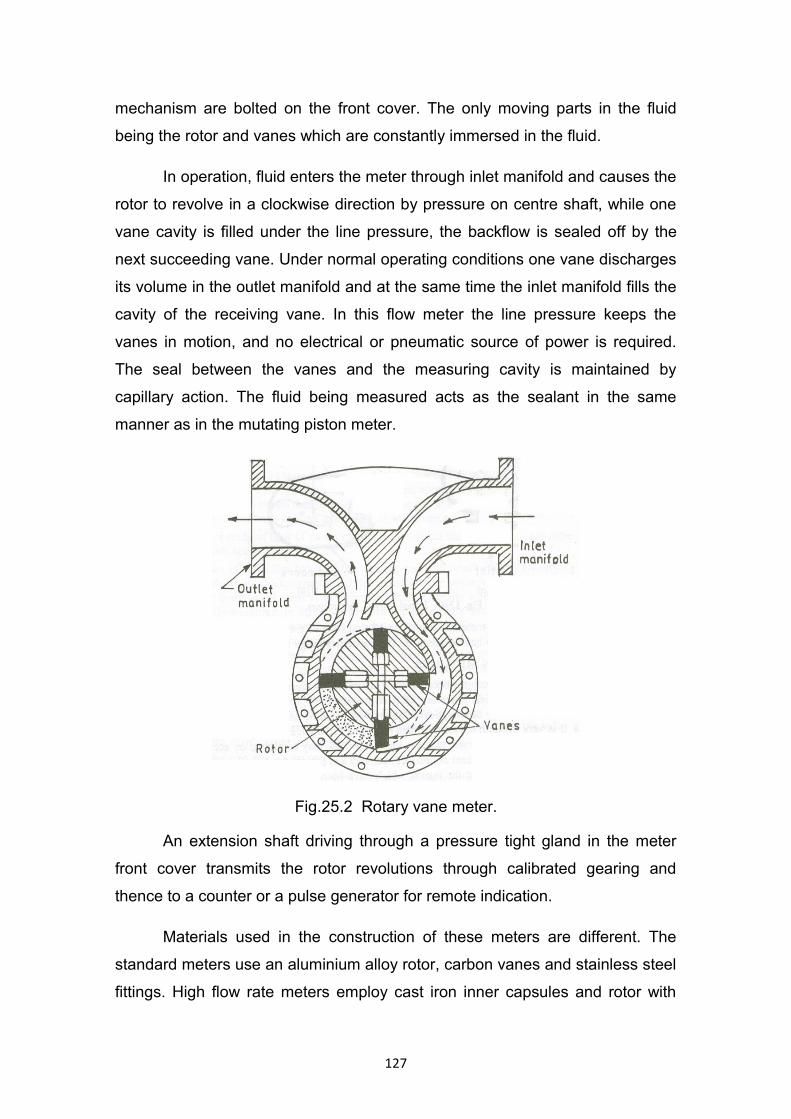
mechanism are bolted on the front cover. The only moving parts in the fluid

being the rotor and vanes which are constantly immersed in the fluid.

In operation, fluid enters the meter through inlet manifold and causes the

rotor to revolve in a clockwise direction by pressure on centre shaft, while one

vane cavity is filled under the line pressure, the backflow is sealed off by the

next succeeding vane. Under normal operating conditions one vane discharges

its volume in the outlet manifold and at the same time the inlet manifold fills the

cavity of the receiving vane. In this flow meter the line pressure keeps the

vanes in motion, and no electrical or pneumatic source of power is required.

The seal between the vanes and the measuring cavity is maintained by

capillary action. The fluid being measured acts as the sealant in the same

manner as in the mutating piston meter.

Fig.25.2 Rotary vane meter.

An extension shaft driving through a pressure tight gland in the meter

front cover transmits the rotor revolutions through calibrated gearing and

thence to a counter or a pulse generator for remote indication.

Materials used in the construction of these meters are different. The

standard meters use an aluminium alloy rotor, carbon vanes and stainless steel

fittings. High flow rate meters employ cast iron inner capsules and rotor with

127

plastic tipped metal vanes, the other parts are made of stainless steel and

brass.

128

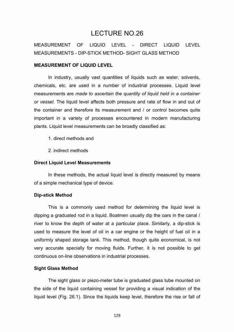
LECTURE NO.26

MEASUREMENT OF LIQUID LEVEL - DIRECT LIQUID LEVEL

MEASUREMENTS - DIP-STICK METHOD- SIGHT GLASS METHOD

MEASUREMENT OF LIQUID LEVEL

In industry, usually vast quantities of liquids such as water, solvents,

chemicals, etc. are used in a number of industrial processes. Liquid level

measurements are made to ascertain the quantity of liquid held in a container

or vessel. The liquid level affects both pressure and rate of flow in and out of

the container and therefore its measurement and / or control becomes quite

important in a variety of processes encountered in modern manufacturing

plants. Liquid level measurements can be broadly classified as:

1. direct methods and

2. indirect methods

Direct Liquid Level Measurements

In these methods, the actual liquid level is directly measured by means

of a simple mechanical type of device.

Dip-stick Method

This is a commonly used method for determining the liquid level is

dipping a graduated rod in a liquid. Boatmen usually dip the oars in the canal /

river to know the depth of water at a particular place. Similarly, a dip-stick is

used to measure the level of oil in a car engine or the height of fuel oil in a

uniformly shaped storage tank. This method, though quite economical, is not

very accurate specially for moving fluids. Further, it is not possible to get

continuous on-line observations in industrial processes.

Sight Glass Method

The sight glass or piezo-meter tube is graduated glass tube mounted on

the side of the liquid containing vessel for providing a visual indication of the

liquid level (Fig. 26.1). Since the liquids keep level, therefore the rise or fall of

129

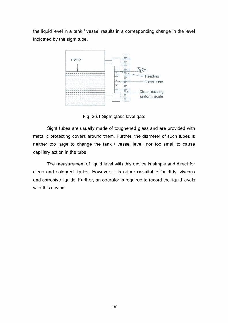
the liquid level in a tank / vessel results in a corresponding change in the level

indicated by the sight tube.

Fig. 26.1 Sight glass level gate

Sight tubes are usually made of toughened glass and are provided with

metallic protecting covers around them. Further, the diameter of such tubes is

neither too large to change the tank / vessel level, nor too small to cause

capillary action in the tube.

The measurement of liquid level with this device is simple and direct for

clean and coloured liquids. However, it is rather unsuitable for dirty, viscous

and corrosive liquids. Further, an operator is required to record the liquid levels

with this device.

130

LECTURE NO.27

HOOK GAUGE- FLOAT GAUGE - FLOAT-AND-SHAFT LIQUID LEVEL

GAUGE

Hook Gauge

Sometimes it becomes necessary to accurately measure very small

changes in liquid level in open tanks / containers. In a large tank / reservoir, a

small change in level would mean large volumetric changes. For such

applications, a simple hook gage is quite suitable. The schematic arrangement

of this gauge is shown in Fig. 27.1. In this device, a vertical tubular rod is

provided with a vernier scale to be clamped at a suitable height at the upper

end and a V-shaped hook at the lower end. This rod moves in a guide bracket

fixed to a rigid body at the datum or reference level and has a main graduated

scale in it. The movable rod is brought downwards so that the hook is first

pushed below the surface of the liquid. It is then gradually raised until the top of

the hook breaks through the surface of the liquid. The movable rod is then

clamped and the level is read off the scale. The device is accurate up to 1.0±

mm, the least count of the instrument. Further, the device is manually operated

and does not lend itself to automatic reading.

Fig. 27.1 Hook type level indicator

Float Gauge

131

A floating body, because of its buoyancy, would always follow the

varying liquid level. Therefore, float-operated devices are capable of giving

continuous, direct liquid level measurements. The floats generally used are

hollow metal spheres, cylindrical ceramic floats or / disc shaped floats of

synthetic materials. The top of the float is usually made sloping so that any

solid suspensions in the liquid do not settle on the float and change its weight.

Float gauges are sufficiently accurate when properly calibrated after

installation. Further, a proper correction is required if there is a change in the

liquid density due to a change in temperature.

Fig.27.2 Float and chain liquid level gauge

Figure 27.2 illustrates a typical float-and-chain liquid level gauge

generally used for directly measuring the liquid level in open tanks. The

instrument consists of a float, a counter weight and a flexible connection that

may be a chain or a thin metallic perforated tape. The counter weight keeps the

chain / tape taut as the liquid rises or falls with any changes in the liquid level.

The chain / perforated tape link is wound on a gear or sprocket wheel to which

the pointer is attached. Any movement of this wheel would indicate on a

suitably calibrated scale the level of the liquid in the tank.

Float-and-Shaft Liquid Level Gauge

Another version of the float-actuated instrument is the float-and-shaft

liquid level gauge (Fig.27.3). In this unit, the motion of the float on the surface

of the liquid is transferred to the shaft and the level is indicated by the pointer

on the dial.

132

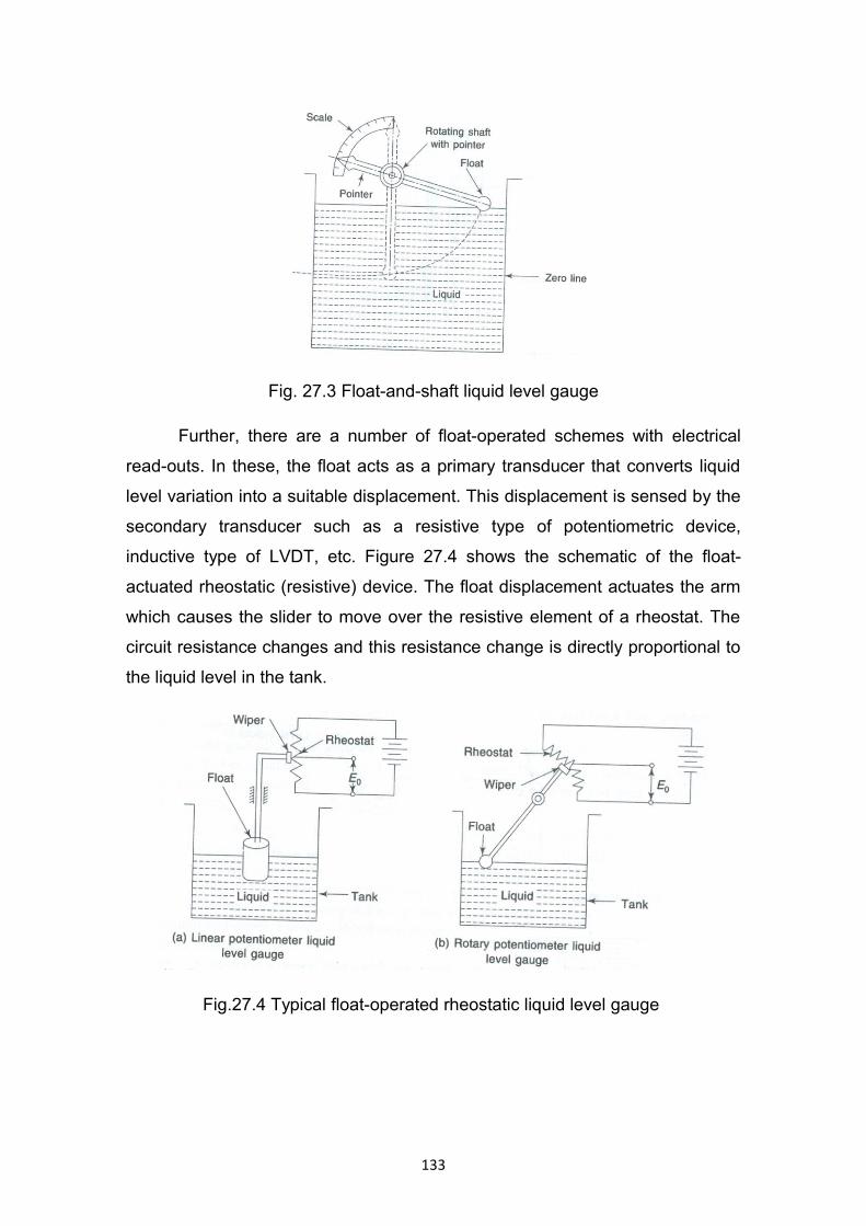
Fig. 27.3 Float-and-shaft liquid level gauge

Further, there are a number of float-operated schemes with electrical

read-outs. In these, the float acts as a primary transducer that converts liquid

level variation into a suitable displacement. This displacement is sensed by the

secondary transducer such as a resistive type of potentiometric device,

inductive type of LVDT, etc. Figure 27.4 shows the schematic of the float-

actuated rheostatic (resistive) device. The float displacement actuates the arm

which causes the slider to move over the resistive element of a rheostat. The

circuit resistance changes and this resistance change is directly proportional to

the liquid level in the tank.

Fig.27.4 Typical float-operated rheostatic liquid level gauge

133

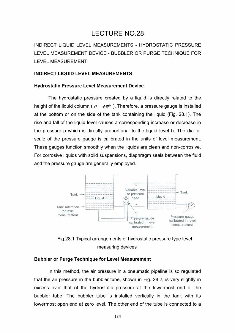
LECTURE NO.28

INDIRECT LIQUID LEVEL MEASUREMENTS - HYDROSTATIC PRESSURE

LEVEL MEASUREMENT DEVICE - BUBBLER OR PURGE TECHNIQUE FOR

LEVEL MEASUREMENT

INDIRECT LIQUID LEVEL MEASUREMENTS

Hydrostatic Pressure Level Measurement Device

The hydrostatic pressure created by a liquid is directly related to the

height of the liquid column ( ghp ρ= ). Therefore, a pressure gauge is installed

at the bottom or on the side of the tank containing the liquid (Fig. 28.1). The

rise and fall of the liquid level causes a corresponding increase or decrease in

the pressure p which is directly proportional to the liquid level h. The dial or

scale of the pressure gauge is calibrated in the units of level measurement.

These gauges function smoothly when the liquids are clean and non-corrosive.

For corrosive liquids with solid suspensions, diaphragm seals between the fluid

and the pressure gauge are generally employed.

Fig.28.1 Typical arrangements of hydrostatic pressure type level

measuring devices

Bubbler or Purge Technique for Level Measurement

In this method, the air pressure in a pneumatic pipeline is so regulated

that the air pressure in the bubbler tube, shown in Fig. 28.2, is very slightly in

excess over that of the hydrostatic pressure at the lowermost end of the

bubbler tube. The bubbler tube is installed vertically in the tank with its

lowermost open end at zero level. The other end of the tube is connected to a

134

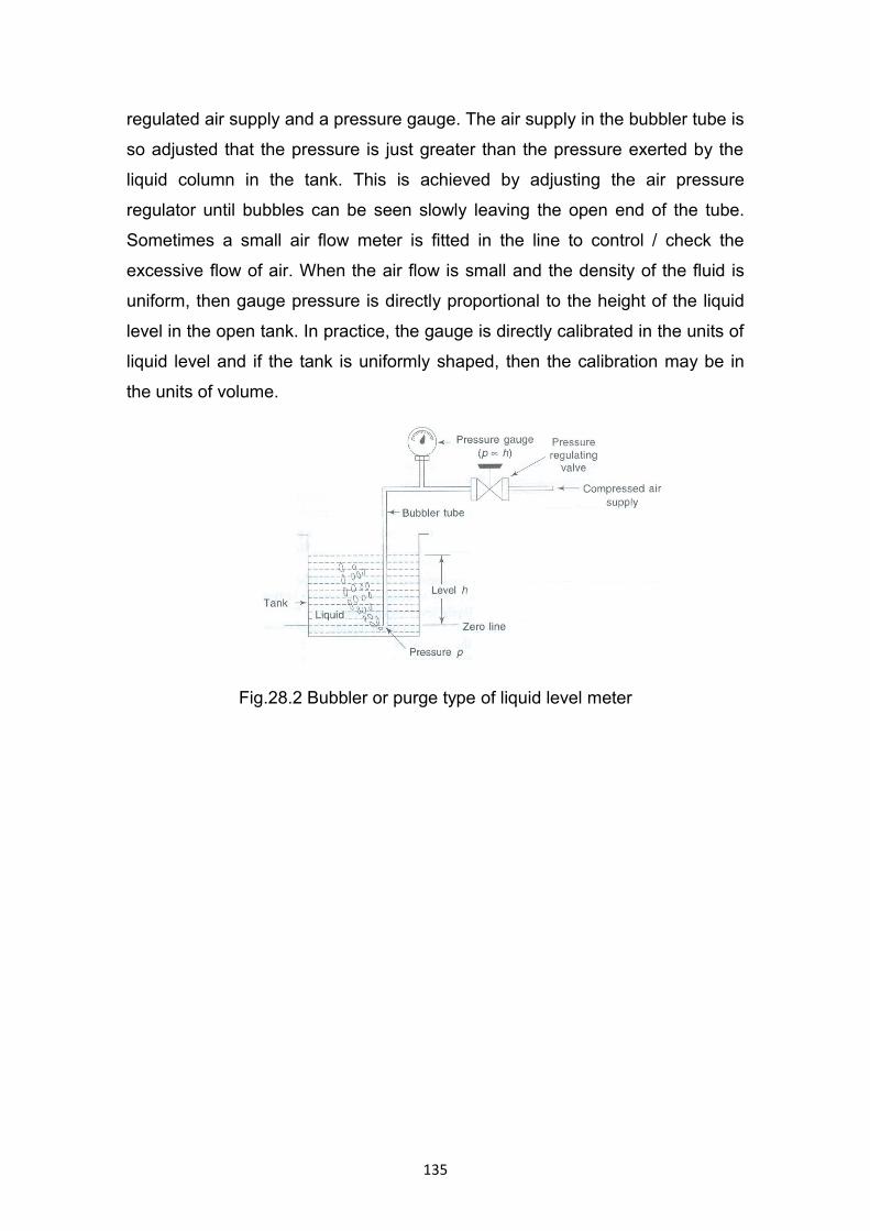
regulated air supply and a pressure gauge. The air supply in the bubbler tube is

so adjusted that the pressure is just greater than the pressure exerted by the

liquid column in the tank. This is achieved by adjusting the air pressure

regulator until bubbles can be seen slowly leaving the open end of the tube.

Sometimes a small air flow meter is fitted in the line to control / check the

excessive flow of air. When the air flow is small and the density of the fluid is

uniform, then gauge pressure is directly proportional to the height of the liquid

level in the open tank. In practice, the gauge is directly calibrated in the units of

liquid level and if the tank is uniformly shaped, then the calibration may be in

the units of volume.

Fig.28.2 Bubbler or purge type of liquid level meter

135

LECTURE NO.29

CAPACITANCE LEVEL GAUGE - ULTRASONIC LEVEL GAUGE -

NUCLEONIC GAUGE

Capacitance Level Gauge

A simple condenser / capacitor consist of two electrode plates separated

by a small thickness of an insulator (which can be solid, liquid, gas or vacuum)

called the dielectric. The change in liquid level causes a variation in the

dielectric between the two plates, which in turn causes a corresponding change

in the value of the capacitance of the condenser. Therefore, such a gauge is

also termed a dielectric level gauge.

The magnitude of the capacitance depends on the nature of the

dielectric, varies directly with the area of the plate and inversely with the

distance between them. The capacitance can be changed by any of these

factors.

In a parallel plate condenser which has identical plates each of area A

(cm2) separated by a distance d (cm) and an insulating medium with dielectric

constant K (K = 1 for air) between them, the expression for the capacitance is

given by

Kd

AFinC 0885.0)( =µµ

From the above equation it is observed that the capacitance varies

directly with the dielectric constant which in turn varies directly with the

liquid level between the plates. Figure 29.1 shows the schematic

arrangement of a capacitance level gauge. The capacitance would be at a

minimum when the tubes contain only air and at a maximum when the liquid

fills the entire space between the electrodes. The change in capacitance can

be measured by a suitable measuring unit such as a capacitive Wheatstone

bridge by either manual null balancing or automatic null balancing using the null

detecting circuit with a servo-motor that indicates the level reading.

136

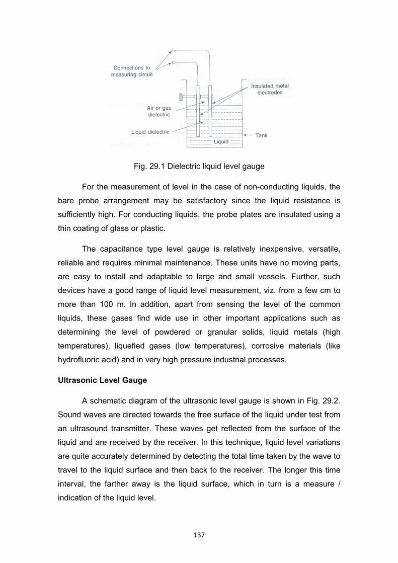
Fig. 29.1 Dielectric liquid level gauge

For the measurement of level in the case of non-conducting liquids, the

bare probe arrangement may be satisfactory since the liquid resistance is

sufficiently high. For conducting liquids, the probe plates are insulated using a

thin coating of glass or plastic.

The capacitance type level gauge is relatively inexpensive, versatile,

reliable and requires minimal maintenance. These units have no moving parts,

are easy to install and adaptable to large and small vessels. Further, such

devices have a good range of liquid level measurement, viz. from a few cm to

more than 100 m. In addition, apart from sensing the level of the common

liquids, these gases find wide use in other important applications such as

determining the level of powdered or granular solids, liquid metals (high

temperatures), liquefied gases (low temperatures), corrosive materials (like

hydrofluoric acid) and in very high pressure industrial processes.

Ultrasonic Level Gauge

A schematic diagram of the ultrasonic level gauge is shown in Fig. 29.2.

Sound waves are directed towards the free surface of the liquid under test from

an ultrasound transmitter. These waves get reflected from the surface of the

liquid and are received by the receiver. In this technique, liquid level variations

are quite accurately determined by detecting the total time taken by the wave to

travel to the liquid surface and then back to the receiver. The longer this time

interval, the farther away is the liquid surface, which in turn is a measure /

indication of the liquid level.

137

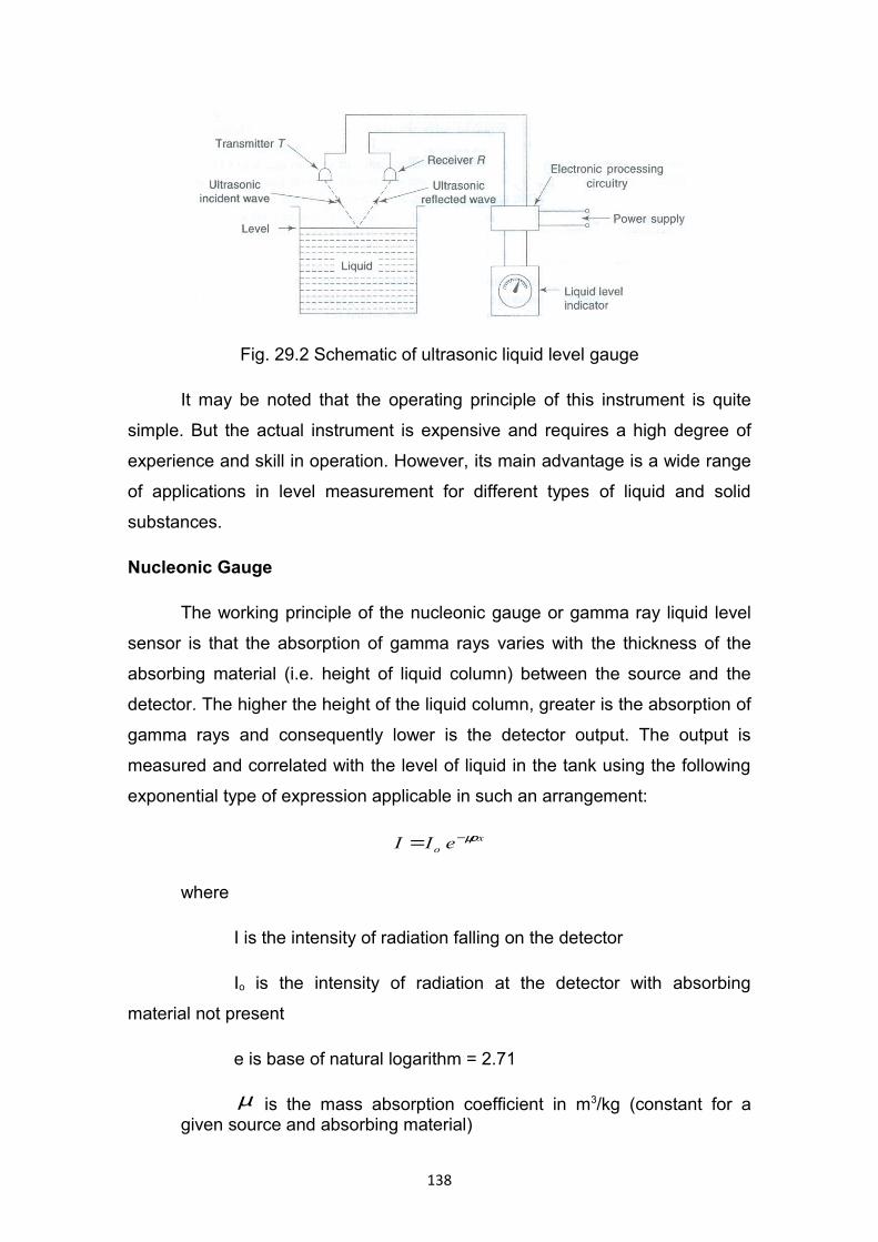
Fig. 29.2 Schematic of ultrasonic liquid level gauge

It may be noted that the operating principle of this instrument is quite

simple. But the actual instrument is expensive and requires a high degree of

experience and skill in operation. However, its main advantage is a wide range

of applications in level measurement for different types of liquid and solid

substances.

Nucleonic Gauge

The working principle of the nucleonic gauge or gamma ray liquid level

sensor is that the absorption of gamma rays varies with the thickness of the

absorbing material (i.e. height of liquid column) between the source and the

detector. The higher the height of the liquid column, greater is the absorption of

gamma rays and consequently lower is the detector output. The output is

measured and correlated with the level of liquid in the tank using the following

exponential type of expression applicable in such an arrangement:

xo eII µρ−=

where

I is the intensity of radiation falling on the detector

Io is the intensity of radiation at the detector with absorbing

material not present

e is base of natural logarithm = 2.71

µ is the mass absorption coefficient in m3/kg (constant for a given source and absorbing material)

138

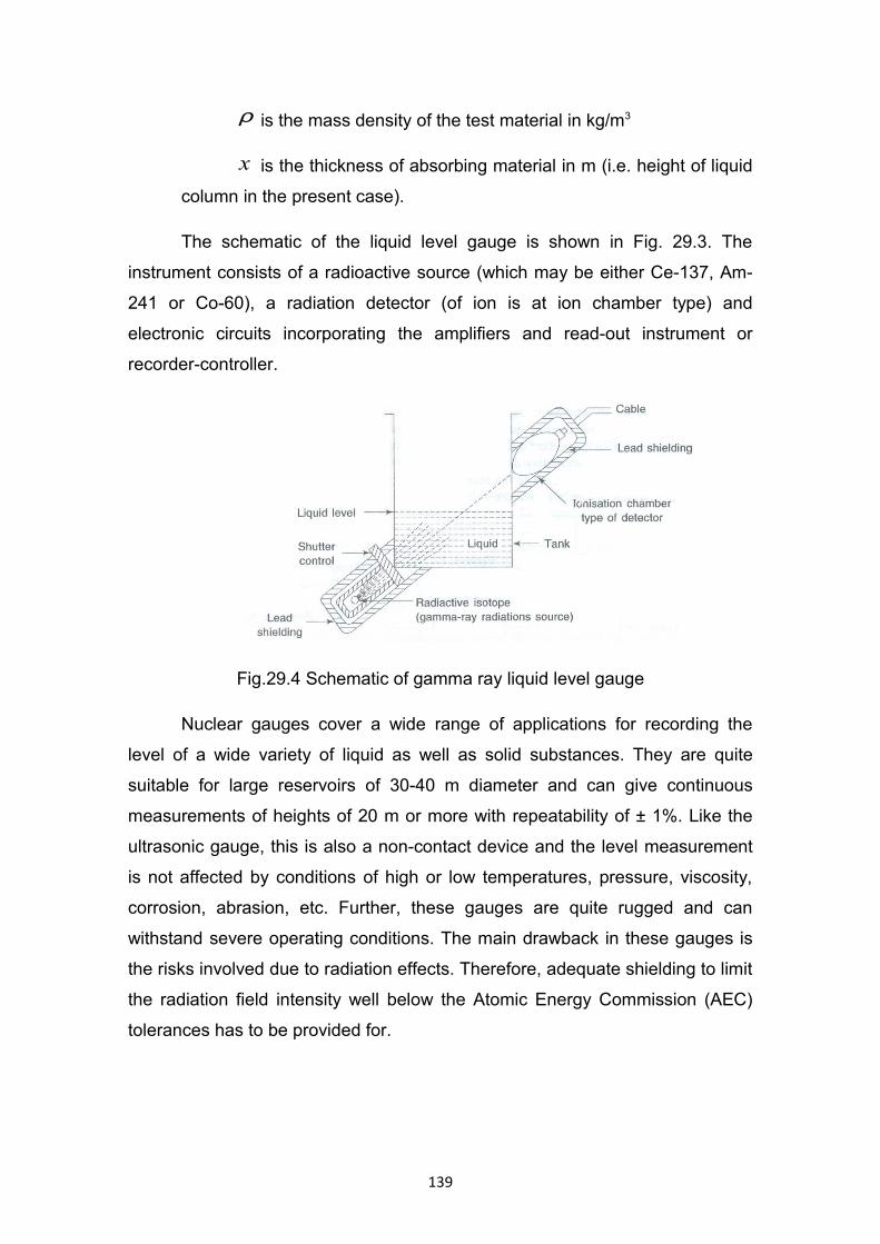
ρ is the mass density of the test material in kg/m3

x is the thickness of absorbing material in m (i.e. height of liquid

column in the present case).

The schematic of the liquid level gauge is shown in Fig. 29.3. The

instrument consists of a radioactive source (which may be either Ce-137, Am-

241 or Co-60), a radiation detector (of ion is at ion chamber type) and

electronic circuits incorporating the amplifiers and read-out instrument or

recorder-controller.

Fig.29.4 Schematic of gamma ray liquid level gauge

Nuclear gauges cover a wide range of applications for recording the

level of a wide variety of liquid as well as solid substances. They are quite

suitable for large reservoirs of 30-40 m diameter and can give continuous

measurements of heights of 20 m or more with repeatability of ± 1%. Like the

ultrasonic gauge, this is also a non-contact device and the level measurement

is not affected by conditions of high or low temperatures, pressure, viscosity,

corrosion, abrasion, etc. Further, these gauges are quite rugged and can

withstand severe operating conditions. The main drawback in these gauges is

the risks involved due to radiation effects. Therefore, adequate shielding to limit

the radiation field intensity well below the Atomic Energy Commission (AEC)

tolerances has to be provided for.

139

LECTURE NO.30

CONTROL SYSTEMS- INTRODUCTION- BASIC COMPONENTS OF THE

CONTROL SYSTEM- CLASSIFICATION OF CONTROL SYSTEMS – OPEN

LOOP SYSTEM - CLOSED LOOP SYSTEM - SERVO MECHANISMS

CONTROL SYSTEMS

Introduction

Automatic control is the maintenance of a desired value of quantity or

condition by measuring the existing value, compare it with the desired value

and employing the difference to initiate action for reducing this difference.

Automatic control systems are used in practically every field of our life.

Since, nowadays it has become a tendency to complete the required work or a

task automatically by reducing the physical and mental effort. The different

applications of automatic control systems are:

1. Domestically they are used in heating and air conditioning.

2. Industrial applications of automatic control system includes:

(i) Automatic control of machine tool operations.

(ii) Automatic assembly lines.

(iii) Quality control, inventory control.

(iv)In process industries such as food, petroleum, chemical, steel,

power etc. for the control of temperature, pressure, flow etc.

(v) Transportation systems, robotics, power systems also uses

automatic control for their operation and control.

(vi) Compressors, pumps, refrigerators.

(vii) Automatic control systems are also used in space technology

and defence applications such as nuclear power weapons, guided

missiles etc.

140

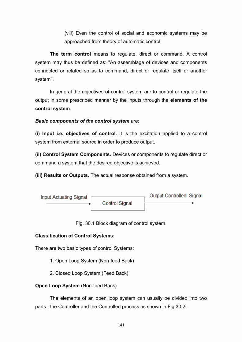
(viii) Even the control of social and economic systems may be

approached from theory of automatic control.

The term control means to regulate, direct or command. A control

system may thus be defined as: "An assemblage of devices and components

connected or related so as to command, direct or regulate itself or another

system".

In general the objectives of control system are to control or regulate the

output in some prescribed manner by the inputs through the elements of the

control system.

Basic components of the control system are:

(i) Input i.e. objectives of control. It is the excitation applied to a control

system from external source in order to produce output.

(ii) Control System Components. Devices or components to regulate direct or

command a system that the desired objective is achieved.

(iii) Results or Outputs. The actual response obtained from a system.

Fig. 30.1 Block diagram of control system.

Classification of Control Systems:

There are two basic types of control Systems:

1. Open Loop System (Non-feed Back)

2. Closed Loop System (Feed Back)

Open Loop System (Non-feed Back)

The elements of an open loop system can usually be divided into two

parts : the Controller and the Controlled process as shown in Fig.30.2.

141

Fig.30.2 Open loop system

An input signal or command r (t) is applied to the controller which

generates the actuating signal u(t).

Actuating signal u(t) then controls (activates) the process to give

controlled output c(t). In simple cases, the controller can be an amplifier,

mechanical linkage, filter, or other control element, depending on the

nature of the system. In more sophisticated cases the controller can be a

computer such as microprocessor.

The control action has nothing to do with output c (t) i.e. there is no any

relation between input and output.

There is no feed back hence it is known as non-feedback system.

Examples of open loop System:

1. Traffic control signals at roadway intersections are the open loop

systems. The glowing of red and green lamps represents the input.

When the red lamp grows the traffic stops. When green lamp glows, it

directs the traffic to start.

The red and green light travels are predetermined by a calibrated

timing mechanism and are in no way influenced by the volume of traffic

(output).

2. Automatic washing machine: In washing machine, input is dirty

clothes, water, soap and output is clean cloths. Soaking, washing and

rinsing operations are carried out on a time basis. However, the machine

does not measure the output signal, namely the cleanliness of the

clothes.

Advantages of Open Loop System:

1. Simple in construction.

2. Economic.

142

3. More stable.

4. Easy maintenance.

Disadvantages of Open Loop System:

1. Inaccurate and unreliable.

2. It is affected by internal and external disturbances, the output may

differ from the desired value.

3. It needs frequent and careful calibrations for accurate results.

4. Open loop systems are slow because they are manually controlled.

5. There is no feed back control. The control systems are rather

unsophisticated.

Closed Loop System

A closed loop control system measures the system output compares it

with the input and determines the error, which is then used in controlling the

system output to get the desired value.

In closed loop system for more accurate and more adaptive control a link

or feedback from the output to the input of the system is provided. The

controlled signal c(t) is fed back and compared with the reference input r(t), an

actuating signal e(t) proportional to the difference of the input and the output is

send through the system to correct the error and bring the system output to the

desired value. The system operation is continually correcting any error that may

exit. As long as the output does not coincide with the desired value, there is

likely to some kind of actuating signal.

Thus, the closed loop systems correct the drifts of the output which may

be present due to external disturbance or due to deterioration of the system

itself.

The closed loop system may have one or more feedback paths. Fig.30.3

shows the general block diagram of closed loop system.

143

Fig. 30.3 Closed loop system

r(t) = reference input

e(t) = error or actuating signal

b(t) = feedback signal

m = manipulation

Advantages of Closed Loop System:

These systems can be used in hazardous or remote areas, such as

chemical plants, fertilizer plants, areas with high nuclear radiations, and

places at very high or very low temperatures.

Increased productivity

Relief of human beings from hard physical work and economy in

operating cost.

Improvement in the quality and quantity of the products.

They are more reliable than human operators.

A number of variables can be handled simultaneously by closed loop

control systems.

In such systems there is reduced effect of non-linearities and distortions.

Closed loop systems can be adjusted to optimum control performance.

Such systems senses environmental changes, as well as internal

disturbances and accordingly modifies the error.

Satisfactory response over a wide range of input frequencies.

Disadvantages of Closed Loop Control System:

It is more complex and expensive.

144

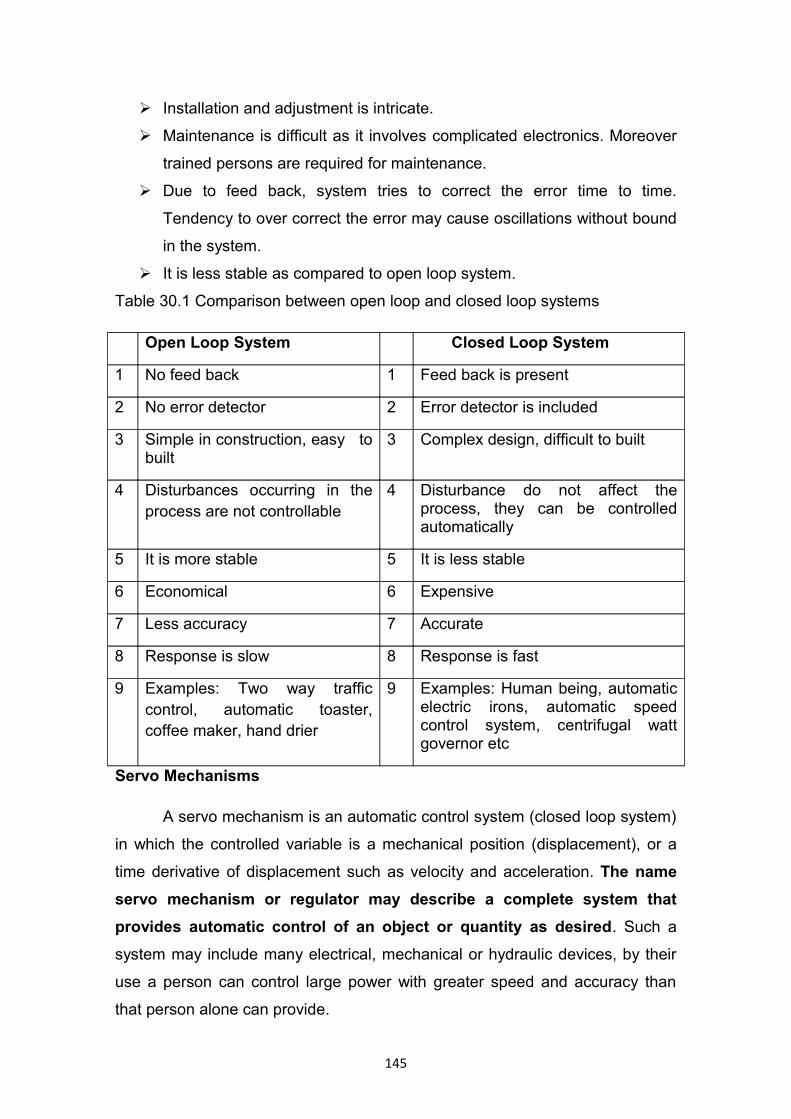
Installation and adjustment is intricate.

Maintenance is difficult as it involves complicated electronics. Moreover

trained persons are required for maintenance.

Due to feed back, system tries to correct the error time to time.

Tendency to over correct the error may cause oscillations without bound

in the system.

It is less stable as compared to open loop system.

Table 30.1 Comparison between open loop and closed loop systems

Open Loop System Closed Loop System

1 No feed back 1 Feed back is present

2 No error detector 2 Error detector is included

3 Simple in construction, easy to built

3 Complex design, difficult to built

4 Disturbances occurring in the process are not controllable

4 Disturbance do not affect the process, they can be controlled automatically

5 It is more stable 5 It is less stable

6 Economical 6 Expensive

7 Less accuracy 7 Accurate

8 Response is slow 8 Response is fast

9 Examples: Two way traffic control, automatic toaster, coffee maker, hand drier

9 Examples: Human being, automatic electric irons, automatic speed control system, centrifugal watt governor etc

Servo Mechanisms

A servo mechanism is an automatic control system (closed loop system)

in which the controlled variable is a mechanical position (displacement), or a

time derivative of displacement such as velocity and acceleration. The name

servo mechanism or regulator may describe a complete system that

provides automatic control of an object or quantity as desired. Such a

system may include many electrical, mechanical or hydraulic devices, by their

use a person can control large power with greater speed and accuracy than

that person alone can provide.

145

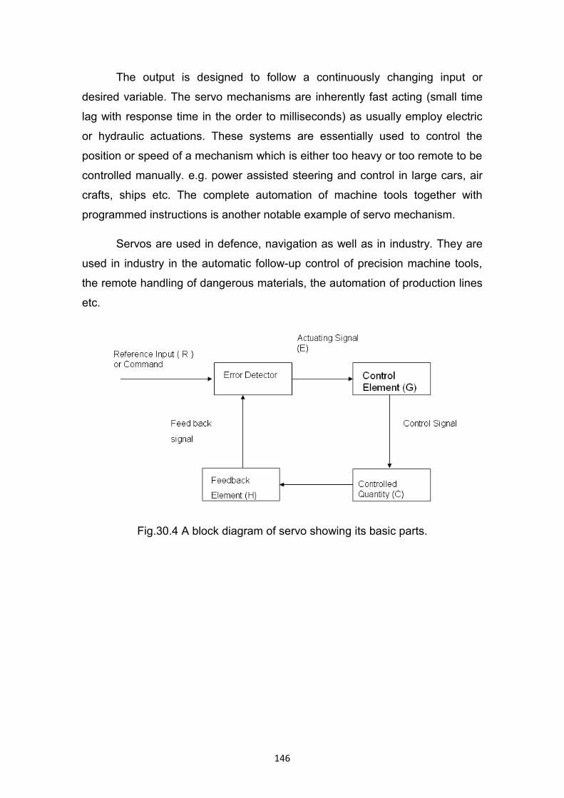
The output is designed to follow a continuously changing input or

desired variable. The servo mechanisms are inherently fast acting (small time

lag with response time in the order to milliseconds) as usually employ electric

or hydraulic actuations. These systems are essentially used to control the

position or speed of a mechanism which is either too heavy or too remote to be

controlled manually. e.g. power assisted steering and control in large cars, air

crafts, ships etc. The complete automation of machine tools together with

programmed instructions is another notable example of servo mechanism.

Servos are used in defence, navigation as well as in industry. They are

used in industry in the automatic follow-up control of precision machine tools,

the remote handling of dangerous materials, the automation of production lines

etc.

Fig.30.4 A block diagram of servo showing its basic parts.

146

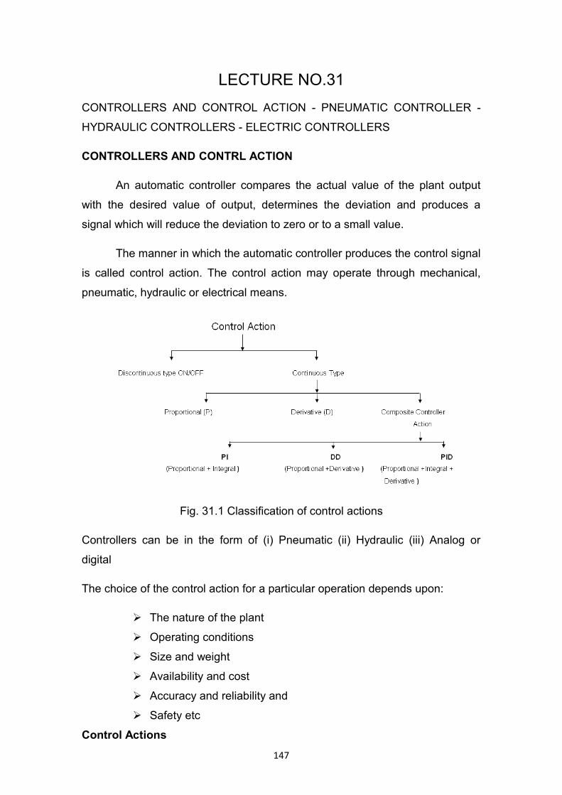
LECTURE NO.31

CONTROLLERS AND CONTROL ACTION - PNEUMATIC CONTROLLER -

HYDRAULIC CONTROLLERS - ELECTRIC CONTROLLERS

CONTROLLERS AND CONTRL ACTION

An automatic controller compares the actual value of the plant output

with the desired value of output, determines the deviation and produces a

signal which will reduce the deviation to zero or to a small value.

The manner in which the automatic controller produces the control signal

is called control action. The control action may operate through mechanical,

pneumatic, hydraulic or electrical means.

Fig. 31.1 Classification of control actions

Controllers can be in the form of (i) Pneumatic (ii) Hydraulic (iii) Analog or

digital

The choice of the control action for a particular operation depends upon:

The nature of the plant

Operating conditions

Size and weight

Availability and cost

Accuracy and reliability and

Safety etc

Control Actions

147

ON-OFF or two position control action

The controller is ON when the measured value is below set point and the

output is at maximum level. When the measured value is above the set point

the controller is OFF and the output is minimum i.e. zero.

These are relatively simple and economical. ON -OFF controllers are

widely used in both industrial and domestic control systems. These controllers

are not suitable for complex systems. The examples of their applications are:

Room heaters, Refrigerators, mixers or food processors, level control of water

tanks etc.

Proportional Control Action (P)

Proportional control action is a continuous mode of operation. In

proportional control, the output changes with proportional change of input. It is

widely used control action where the output of controller is a linear function of

error signal.

The proportional control follows the law :

0)()( Ptekptm +=

where,

=)(tm controller output

=)(te error signal

=kp gain of controller

=0P output of controller when error is zero

The proportional controller may be thought of as an amplifier with high

and adjustable gain.

Composite Control Action

Composite control action means combination of two continuous control action:

1. Proportional Plus Integral Control Action (P + I)

148

The proportional control action produces off set in the system whenever

load change occurs. This offset can be eliminated by adding integral action to

the proportional control action. The output is

0

0

.)()()( PdtteTi

kptekptm

T

++= ∫

2. Proportional Plus Derivative (PD) Control Action

In a derivative control mode, the magnitude of the controller output is

proportional to the rate of change of the actuating error signal. The control

action in which derivative control action is added to the proportional control

action is called PD control action.

The governing equation of PD control action is

0

)(.)()( P

dt

tedTdkptekptm ++=

Advantages: Improves damping ratio and reduces maximum overshoot.

3. PID Control Action: It is powerful but complex control action. In a PID

control action, the output m(t) is a linear combination of input e(t), the time rate

of change of input and the time integral of input. The control is thus an additive

combination of proportional action, derivative action, and integral action.

The equation of PID control action is given by

0.)( PdteTd

kp

dt

edTdkpekptm +++= ∫

PNEUMATIC CONTROLLER

Pneumatic controllers use air medium (or other gases in special

situations) to provide an output signal which is a function of an input error

signal. Regulated pressurized air supply at about 20 psg is used as a input

signal. Air medium has the advantage of being non-inflammable and having

almost negligible viscosity compared to the high viscosity of hydraulic fluids.

The danger of explosion existed due to electrical equipment is avoided by

pneumatic controller.

149

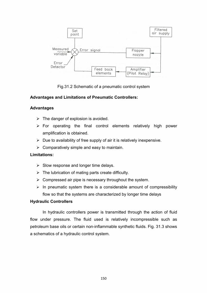
Fig.31.2 Schematic of a pneumatic control system

Advantages and Limitations of Pneumatic Controllers:

Advantages

The danger of explosion is avoided.

For operating the final control elements relatively high power

amplification is obtained.

Due to availability of free supply of air it is relatively inexpensive.

Comparatively simple and easy to maintain.

Limitations:

Slow response and longer time delays.

The lubrication of mating parts create difficulty.

Compressed air pipe is necessary throughout the system.

In pneumatic system there is a considerable amount of compressibility

flow so that the systems are characterized by longer time delays

Hydraulic Controllers

In hydraulic controllers power is transmitted through the action of fluid

flow under pressure. The fluid used is relatively incompressible such as

petroleum base oils or certain non-inflammable synthetic fluids. Fig. 31.3 shows

a schematics of a hydraulic control system.

150

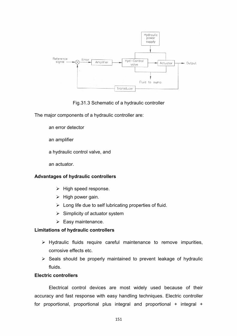
Fig.31.3 Schematic of a hydraulic controller

The major components of a hydraulic controller are:

an error detector

an amplifier

a hydraulic control valve, and

an actuator.

Advantages of hydraulic controllers

High speed response.

High power gain.

Long life due to self lubricating properties of fluid.

Simplicity of actuator system

Easy maintenance.

Limitations of hydraulic controllers

Hydraulic fluids require careful maintenance to remove impurities,

corrosive effects etc.

Seals should be properly maintained to prevent leakage of hydraulic

fluids.

Electric controllers

Electrical control devices are most widely used because of their

accuracy and fast response with easy handling techniques. Electric controller

for proportional, proportional plus integral and proportional + integral +

151

derivative actions may be divided into two types: (1) The null balance type in

which an electrical feedback signal is given to the controller from the final

elements.

(2) The direct type in which there is no such feedback signal.

As with the pneumatic controller, the various control actions are

accomplished by modifying the feed back signal. This is done by adding

properly combined electrical resistances and capacitances to feedback circuit

just as restrictions and bellows were added in the pneumatic circuit.

A very simple form of two step controller is the room-temperature

thermostat. Fig.31.4 show simple type of electrical two position control. The U

shaped bimetal strip fixed at one end of the thermostat frame deflects when

heated, its free and moving in such a direction as to separate the fixed and

moving contacts. When the bimetal strip cools the two contacts are once more

brought in contact. The small permanent magnet ensures the opening and

closing of the contacts with a snap action to minimize the damage caused by

arcing. The adjusting screw varies the small range of temperature, sometimes

called the differential gap between contacts opening on rising temperature and

closing on falling temperature.

Fig. 31.4 Electrical two position control

152

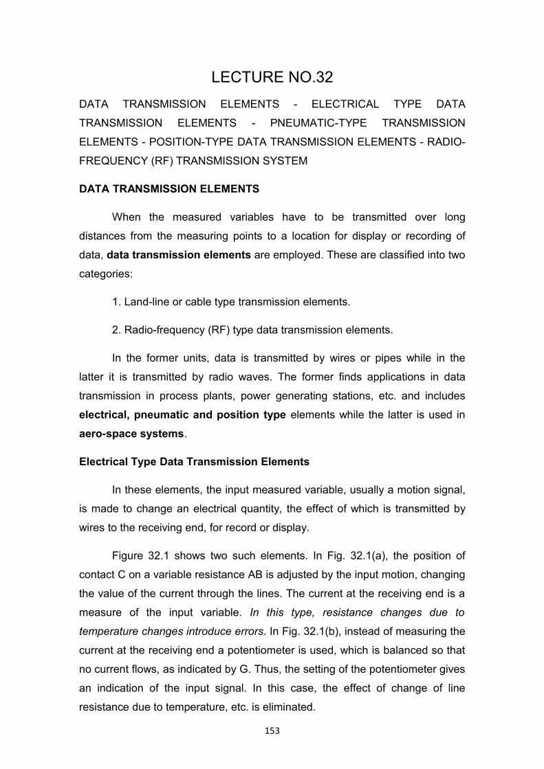
LECTURE NO.32

DATA TRANSMISSION ELEMENTS - ELECTRICAL TYPE DATA

TRANSMISSION ELEMENTS - PNEUMATIC-TYPE TRANSMISSION

ELEMENTS - POSITION-TYPE DATA TRANSMISSION ELEMENTS - RADIO-

FREQUENCY (RF) TRANSMISSION SYSTEM

DATA TRANSMISSION ELEMENTS

When the measured variables have to be transmitted over long

distances from the measuring points to a location for display or recording of

data, data transmission elements are employed. These are classified into two

categories:

1. Land-line or cable type transmission elements.

2. Radio-frequency (RF) type data transmission elements.

In the former units, data is transmitted by wires or pipes while in the

latter it is transmitted by radio waves. The former finds applications in data

transmission in process plants, power generating stations, etc. and includes

electrical, pneumatic and position type elements while the latter is used in

aero-space systems.

Electrical Type Data Transmission Elements

In these elements, the input measured variable, usually a motion signal,

is made to change an electrical quantity, the effect of which is transmitted by

wires to the receiving end, for record or display.

Figure 32.1 shows two such elements. In Fig. 32.1(a), the position of

contact C on a variable resistance AB is adjusted by the input motion, changing

the value of the current through the lines. The current at the receiving end is a

measure of the input variable. In this type, resistance changes due to

temperature changes introduce errors. In Fig. 32.1(b), instead of measuring the

current at the receiving end a potentiometer is used, which is balanced so that

no current flows, as indicated by G. Thus, the setting of the potentiometer gives

an indication of the input signal. In this case, the effect of change of line

resistance due to temperature, etc. is eliminated.

153

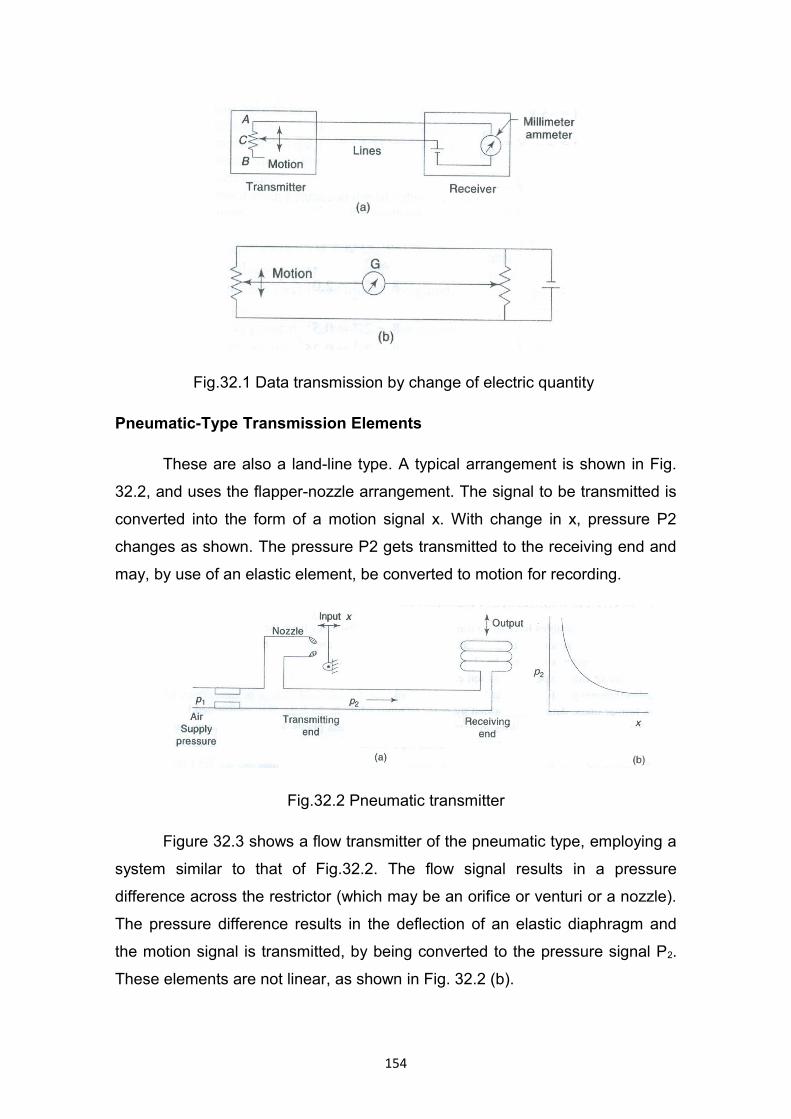
Fig.32.1 Data transmission by change of electric quantity

Pneumatic-Type Transmission Elements

These are also a land-line type. A typical arrangement is shown in Fig.

32.2, and uses the flapper-nozzle arrangement. The signal to be transmitted is

converted into the form of a motion signal x. With change in x, pressure P2

changes as shown. The pressure P2 gets transmitted to the receiving end and

may, by use of an elastic element, be converted to motion for recording.

Fig.32.2 Pneumatic transmitter

Figure 32.3 shows a flow transmitter of the pneumatic type, employing a

system similar to that of Fig.32.2. The flow signal results in a pressure

difference across the restrictor (which may be an orifice or venturi or a nozzle).

The pressure difference results in the deflection of an elastic diaphragm and

the motion signal is transmitted, by being converted to the pressure signal P2.

These elements are not linear, as shown in Fig. 32.2 (b).

154

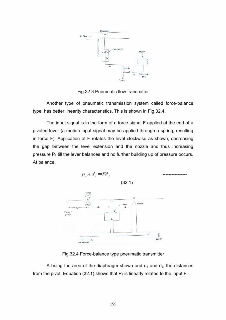
Fig.32.3 Pneumatic flow transmitter

Another type of pneumatic transmission system called force-balance

type, has better linearity characteristics. This is shown in Fig.32.4.

The input signal is in the form of a force signal F applied at the end of a

pivoted lever (a motion input signal may be applied through a spring, resulting

in force F). Application of F rotates the level clockwise as shown, decreasing

the gap between the level extension and the nozzle and thus increasing

pressure P2 till the lever balances and no further building up of pressure occurs.

At balance,

122 FddAp = ----------------

(32.1)

Fig.32.4 Force-balance type pneumatic transmitter

A being the area of the diaphragm shown and d1 and d2, the distances

from the pivot. Equation (32.1) shows that P2 is linearly related to the input F.

155

In pneumatic type transmitters, there is a pressure drop in transmission

piping, resulting in a reduction in the signal transmitted. In practice, these are

used for transmitting the signal over a few hundred meters.

Position-Type Data Transmission Elements

In these types, the motion signal (like rotation of a pointer) is transmitted

over long distances, by use of synchros. Two synchros - a transmitter and a

receiver are employed (Fig.32.5). A synchro consists of a stator with three coils

at 120°, inside which is a rotor, which is free to rotate within the stator windings.

The transmitting synchro is energized by an ac power source. If the two rotors

are in identical positions, the voltages in stators have the same magnitude but

opposite sense and no current flows in the stator wires. If the input rotor is

turned, making the two rotor positions different, current flows in the stator wires

producing a resulting torque which would align the two rotors making io θθ =

.Thus, the angular motion iθ is transmitted to the receiving end.

Fig. 32.5 Synchros for data transmission

Radio-Frequency (RF) Transmission System

Such data transmission systems use radio-frequency waves for data

transmission and no wires or cables are needed between the transmitting and

receiving ends. In large systems like aero-space systems, a number of input

signals like temperature, pressure, vibrations, etc. may be transmitted by such

units.

156