Embed Size (px)
Citation preview
ACHARYA N.G. RANGA AGRICULTURAL UNIVERSITY
B.Tech (Food Technology)
Course No. FDEN-323Course Title: FOOD PLANT DESIGN AND LAYOUTCredits: 3 (2 + 1)
Prepared by
Er. B. SREENIVASULA REDDY
Assistant Professor (Food Engineering)
College of Food Science and Technology
Chinnarangapuram, Pulivendula – 516390
YSR (KADAPA) District, Andhra Pradesh
DEPARTMENT OF FOOD ENGINEERING1 Course No : FDEN - 3232 Title : Food Plant Design and Layout3 Credit hours : 3 (2+1)4 General Objective : To impart knowledge on plant layout and design of
food industries5 Specific Objectives :
a) Theory : By the end of the course, the students will acquire
knowledge on theoretical aspects to be considered
for site selection, layout selection and design
considerations for a food plantb) Practical By the end of the course, the students will develop
skills and acquaint in project preparations,
estimations and cost estimates of different
equipment and utilities of various food industriesA) Theory Lecture Outlines
1 Introduction : Plant design concepts - situations giving rise to plant design
problems - differences in design of food processing and non-food processing
plants2 General design considerations, Food Processing Unit Operations, Prevention
of Contamination, Sanitation, Deterioration, Seasonal Production3 Flow Chart for Plant Design, Identification Stage, Looking for a need, Finding
a product, Preliminary Screening of ideas4 Comparative rating of product ideas: Present Market, Market Growth
potential, Costs, Risks5 Pre Selection / Pre feasibility stage, Analysis Stage: Market Analysis,
Situational analysis related to market6 Technical analysis, Financial Analysis, Sensitivity and risk analysis, Feasibility
cost estimates 7 Break Even Analysis: Introduction, Break-Even Chart, Fixed Costs, Variable
costs, Break even point calculation8 Plant location :Introduction, Location Decision Process, Factors involved in
the plant location decision, 9 Territory selection and Site/ community selection10
Subjective, Qualitative and Semi-Quantitative Techniques, Equal Weights
Method, Variable Weights Method, Weight-cum-Rating Method, Another
weight-cum-rating method11
Composite Measure method, Locational Break-Even analysis
12
Food Plant Utilities: Process Water, Steam, Electricity, Plant Effluents
1 Plant Size and Factors
2
314
The enterprise and its Environment, The total revenue function, the total cost
function15
Break-even and shutdown points, Production, economics of mass production,
Production management decision16
Plant layout : Importance, Flow Patterns
17
Basic Types of plant layouts, Product or line layout, Process or functional
layout, Cellular or group layout, and Fixed position layout, Plant Layout
factors, Layout design Procedure
18
General guide lines for plant layout, Typical clearances, areas and
allowances, Plant layout, Layout of equipment, Space determination19
Symbols used for food plant design and layout: Introduction, valves, line
symbols, fluid handling, heat transfer, Mass transfer20
Symbols used for food plant design and layout: Storage vessels, conveyors
and feeders, separators, mixing and communition and process control and
instrumentation symbols. 21
Experimentation in pilot layout : Size and structure of the pilot plant, minimum
and maximum size, types and applications 22
Engineering Economy : Introduction, Terms: Time value of money, inflation,
Interest, Interest rate, compound interest, rate of return, payment, receipt ,
cash flow, present value, Equivalence, sunk costs, opportunity costs, Asset,
Life of an asset, depreciation, book value of an asset, salvage value,
retirement, replacement, defender and challenger.23
Methods of economic evaluation of engineering alternatives
1. Undiscounted cash flow methods -pay back period method
2. Discounted cash flow methods
a) Net present value method
b) Equivalent annual method
c) Rate of return method
3.Cost- benefit analysis, Social costs, social benefits24
Process scheduling
25
Linear Programming: Introduction, Salient features of Linear programming
(Terminology)26
Formulation of linear programming model, Advantages, limitations and
applications of linear programming, solution of linear programming problems.27
Queuing theory : Introduction, Elements of queuing system, 1) Input source,
2) Queue 2 Queuing theory: Characteristics of waiting lines, service discipline, Service
3
8 mechanism, system out put, customer behavior. 29
Materials of construction of Food Equipment : Characteristics of suitable
construction material : Stainless steel, Aluminum, Nickel and Monel, Plastic
Materials30
Illumination and ventilation
31
Cleaning & sanitization
32
Maintenance of Food Plant Building : Safety Color Code, Roof Inspection,
Care of Concrete floors
B) Practical Class Outlines1 Preparation of project report2 Preparation of feasibility report3 Layout of Food storage wares and godowns4 Layout and design of cold storage5 Layout of preprocessing house6 Layout of Milk and Milk product plants7 Design and layout of low shelf life product plant8 Design and layout of fruits processing plants9 Design and layout of vegetable processing plants10
Layout of multi product and composite food plants
11
Evaluation of given layout
12
Waste treatment and management of food plant
13
Design and layout of modern rice mill
14
Design and layout of mango pulp canning industry
15
Design and layout of spices manufacturing unit
16
Design and layout of Bakery and related product plant
References1 M Moor, Mac Millan, Plant Layout & Design. Lames, New York.2 H.S. Hall & Y.S. Rosen, Milk Plant Layout. FAO Publication, Rome.3 F.W. Farrall, Dairy & Food Engineering. John Willy & Sons, New York.4 Food Plant Design by Antonio López. Gómez5 Food plant engineering systems by Theunis C. Robberts, CRC Press, Washington6 Food plant economics by Zacharias B. Maroulis and George D. Saravacos
published by Taylor and Francis Group, LLC7 Fundamentals of Production Systems Engineering, G.S.Sekhon and A.S.Sachdev,
Published by Dhanpat Rai and Company Private Limited, Delhi (Chapter NO. 19)8 Operations Research by Manohar Mahajan, Published by Dhanpat Rai and
4

Company Private Limited, Delhi9 Food Process Design by Zacharias B. Maroulis published by Marcel Dekker, Inc ,
Cimarron Road, Monticello, New York 12701, U S A
5
LECTURE NO. 1
INTRODUCTION: PLANT DESIGN CONCEPTS - SITUATIONS GIVING RISE
TO PLANT DESIGN PROBLEMS - DIFFERENCES IN DESIGN OF FOOD
PROCESSING AND NON-FOOD PROCESSING PLANTS
INTRODUCTION
Plant design refers to the overall design of a manufacturing enterprise /
facility. It moves through several stages before it is completed. The stages
involved are : identification and selection of the product to be manufactured,
feasibility analysis and appraisal, design, economic evaluation, design report
preparation, procurement of materials including plant and machinery construction,
installation and commissioning. The design should consider the technical and
economic factors, various unit operations involved, existing and potential
market conditions etc.
Plant design specifies:
• the equipment to be used
• performance requirements for the equipment
• interconnections and raw material flows in terms of flow charts
and plant layouts
• the placement of equipment, storage spaces, shop facilities, office
spaces, delivery and shipping facilities, access ways, site plans and
elevation drawings
• required instrumentation and controls, and process monitoring
and control interconnections
• utility and waste treatment requirements, connections and
facilities
• the rationale for site selection
• the basis for selecting and sizing critical pieces of equipment
• ways in which the design was optimized and the engineering basis
for such optimization
They also often provide economic analyses of plant profitability in terms of
various product demand and price and material cost scenarios.
Plant Design Situations
6
Plant design situations may arise due to one or more of the following:
• design and erection of a completely new plant
• design and erection of an addition to the existing plant
• the facility or plant operations and subsequent expansion restricted by a
poor site, thereby necessitating the setting up of the plant at a new
site
• addition of some new product to the existing range
• adoption of some new process /replacement of some existing equipment
• modernization / automation of the existing facility
• expansion of the plant capacity
• relocating the existing plant at a new site because of new economic,
social, legal or political factors
Differences in the Design of Food Processing and Non-Food Processing
Plants
Many of the elements of plant design are the same for food plants as they
are for other plants particularly those processing industrial chemicals. However,
there are many significant differences, basically in the areas of equipment
selection and sizing, and in working space design. These differences stem from
the ways in which the processing of foods differ from the processing of industrial
chemicals.
Such differences occur because of the following considerations:
The storage life of foods is relatively limited and strongly affected by
temperature, pH, water activity, maturity, prior history, and initial microbial
contamination levels.
Very high and verifiable levels of product safety and sterility have to be
provided.
Foods are highly susceptible to microbial attack and insect and rodent
infestation.
Fermentations are used in producing various foods and bio chemicals.
Successful processing requires the use of conditions, which ensure the
dominance of desired strains of microorganisms growth or activity.
Enzyme-catalyzed processes are used or occur in many cases. These, like
microbial growth and fermentation are very sensitive to temperature, pH, water
activity and other environmental conditions.
7
Many foods are still living organisms or biochemically active long after
harvest or slaughter.
In some cases foods (e.g. ripening cheeses) contain active living micro-
organisms, which induce chemical transformations for long periods of time.
Crop-based food raw materials may only be available in usable form on a
seasonal basis. Therefore, plant design may involve the modeling of crop
availability.
Food raw materials are highly variable and that variability is enhanced by
the ageing of raw material and uncontrollable variations in climatic conditions.
The biological and cellular nature and structural complexity of foods causes
special heat-transfer, mass-transfer and component separation problems.
Foods are frequently solid. Heat and mass-transfer problems in solids have
to be created in ways that are different than those used for liquid and gas
streams. The kinetics of microbe and enzyme inactivation during thermally
induced sterilization and blanching and heat-transfer in the solids being sterilized
or blanched are strongly linked.
Food processing generates wastes with high BOD loads.
Foods are often chemically complex systems whose components tend to
react with one another. Certain types of reactions, e.g. Maillard reactions,
oxidative rancidification, hydrolytic rancidification and enzymatic browning tend to
occur with a high degree of frequency.
The engineering properties of foods and biological material are less well
known and more variable than those of pure chemicals and simple mixtures of
chemicals.
Vaguely defined sensory attributes often have to be preserved, generated
or modified. These require sensory testing. Raw material variation, minor
processing changes and trace contaminants leached from processing equipment
and packages can often cause significant changes in these attributes. Frequently,
we do not have mechanistic bases for linking these attributes to processing
conditions and equipment design. Much current food engineering and food
science research activity at universities is designed to provide such linkages.
In the case of foods, prototype products have to be consumer tested so as
to assure market acceptability before plants for large scale production are built.
8
Mechanical working is sometimes used to induce desired textural changes.
Examples include kneading and sponge mixing during the making of bread, the
calendaring of pastry dough, shearing during extrusion texturization.
Packaging in small containers is often used or required; and strong-
package-product interactions exist. Packaging often requires care to maintain
integrity of closure, reproducibility of fill elimination of air from head spaces and
prevention of subsequent moisture and oxygen transfer. Segregation often causes
problems in the packaging of powdered foods. Aseptic packaging is starting to be
widely used.
Food processing techniques and formulations are sometimes constrained
by standards of identity and good manufacturing practice regulations and codes.
Food processing is an art to a certain extent. Engineers and technologists
are frequently uncertain as to weather portions of that art are really justified or
necessary. It is sometimes difficult for them to translate the necessary portions of
that art into quantifiable heat-transfer and chemical reaction processes on which
rational designs can be based.
9
LECTURE NO. 2
GENERAL DESIGN CONSIDERATIONS, FOOD PROCESSING UNIT
OPERATIONS, PREVENTION OF CONTAMINATION, SANITATION,
DETERIORATION, SEASONAL PRODUCTION
General Design Considerations
Food plant designs must provide necessary levels of sanitation, means of
preventing product and material contamination and means of preventing or
limiting product, raw material, and intermediate product deterioration due to
naturally occurring processes. Great care must be exercised to achieve high
levels of product purity and preserve product integrity. A brief description of some
of the design considerations follows.
Food processing unit operations
Food processing involves many conventional unit operations but it also
involves many which differ greatly from those usually encountered in the
production of industrial chemicals. These include: freezing and thawing and other
temperature-induced phase transitions or phase transition analogs, freeze drying,
freeze concentration, curd and gel formation, development of structured gels,
cleaning and washing (the operation which occurs with the greatest frequency in
food processing plants), leavening, puffing, and foaming, slaughtering, carcass
disassembly, component excision, slicing and dicing, peeling and trimming,
grading, cell disruption and maceration, pasteurization and sterilization, blanching,
baking, cooking (for purposes of tenderization or textural modification), roasting
(for purposes of flavour generation), radiation sterilization, mechanical expression,
structure-based component separation, filling and packaging, canning and
bottling, coating and encapsulation, sausage and flexible casing, stuffing,
controlled atmosphere storage, fumigation and smoking, churning, artificially
induced ripening, fermentation, pureeing, emulsification and homogenization,
biological waste treatment, and controlled feeding of confined animals, poultry and
fish.
Prevention of contamination
Prevention of contamination will involve the provision or use of filtered air,
air locks, piping layouts that ensure complete drainage and present cross-stream
contamination (particularly contamination of finished products by unsterilized or
10
unpasteurized raw material and cleaning solutions), solid material and human
traffic flow layouts that also prevent such contamination, suitably high curbs when
pipes, conveyors or equipment pass through floors and where gangways pass
over processing areas, bactericides in cooling water, culinary (i.e. contaminant-
free) steam whenever direct contact between a product and steam is used,
impermeable covers for insulation, dust covers over conveyors and clear plastic
covers for electric lights, methods for washing bottles and containers, suitable
barriers against pest entry, windowless construction, solid instead of hollow walls,
or completely tight enclosure of hollow spaces in walls, air circulation system and
external roof and wall insulation that prevent the formation of condensate which
can drip into products or favor mold growth, ultra-violet irradiation of tank head
spaces, electric light traps for flying insects, impactors for killing insect eggs,
larvae, pupae and adults in grain, carbon dioxide and nitrogen fumigation of dry
food storage bins, screening system to remove insects and insect parts, magnetic
traps, iron screens for sieving equipment (so that screen fragments can be picked
up by magnetic traps), metal detectors for rejecting packaged product that
contains unwanted metal, and methods for storing and keeping track of
segregated batches of raw materials and finished goods until necessary quality
assurance tests have been carried out.
Sanitation
Sanitation, which helps prevent contamination, should be facilitated by
providing or using: impermeable coated or tiled floors and walls, at least one floor
drain per every 40 m2 of wet processing area, special traps for such drains,
pitched floors that ensure good drainage, polished vessels and equipment that do
not contain dead spaces and which can be drained and automatically cleaned in
place, sanitary piping, clean-in-place (CIP) systems, plate heat exchangers and
other types of equipment which can be readily disassembled for cleaning if
necessary, clearances for cleaning under and around equipment, grouting to
eliminate crevices at the base of equipment support posts and building columns,
tubular pedestals instead of support posts constructed from beams, and methods
for removing solid particles which fall off conveyors. Air flow and human traffic
flow patterns should be maintained to eliminate possibilities of containment
transfer from dirty areas to clean ones. Very high levels of sanitation must be
provided for foodstuffs that provide good substrates for the growth of micro-
organisms and when processing temperatures and conditions favor such growth.
11
Deterioration
To minimize product and raw material deterioration, provisions should be
made for: refrigerated and controlled environment storage areas, space and
facilities for product inspection and for carrying out quality assurance tests, surge
vessels for processed material between different operations (particularly
operations which are subject to breakdown), equipment for pre-cooling material
stored in such vessels, means of cooling, turning over or rapidly discharging the
contents of bins and silos when excessive temperature rises, occur, and standby
refrigeration and utility arrangements which are adequate to prevent product and
raw material deterioration in case of power interruptions or unusual climatic
conditions.
Seasonal production
Food plants have to be sized to accommodate peak seasonal flows of
product without excessive delay, and in some cases, have to be highly flexible so
as to handle different types of fruits and vegetables. Modeling of crop and animal
growth processes can be of great help in scheduling production and adequately
sizing plants.
12
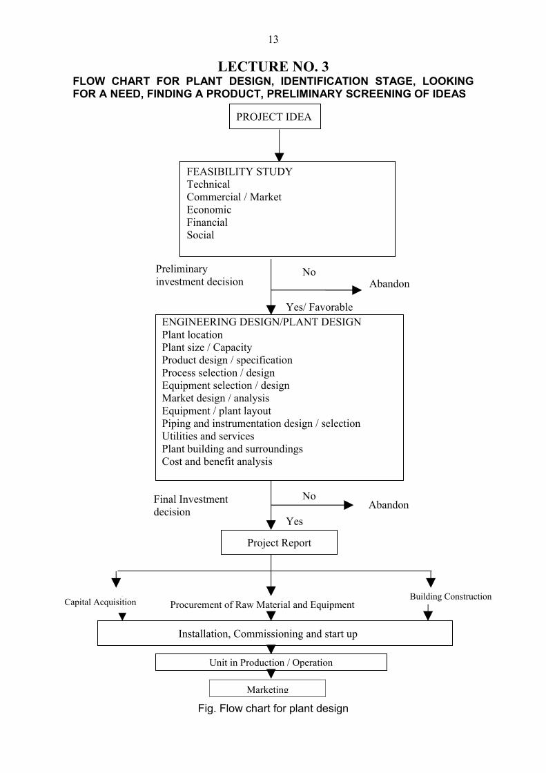
LECTURE NO. 3FLOW CHART FOR PLANT DESIGN, IDENTIFICATION STAGE, LOOKING FOR A NEED, FINDING A PRODUCT, PRELIMINARY SCREENING OF IDEAS
Fig. Flow chart for plant design
FEASIBILITY STUDY Technical Commercial / Market Economic Financial Social
AbandonNo
Yes/ Favorable
Preliminary investment decision
ENGINEERING DESIGN/PLANT DESIGN Plant location Plant size / CapacityProduct design / specification Process selection / design Equipment selection / design Market design / analysis Equipment / plant layout Piping and instrumentation design / selection Utilities and services Plant building and surroundings Cost and benefit analysis
PROJECT IDEA
AbandonNo
Yes
Final Investment decision
Project Report
Procurement of Raw Material and EquipmentBuilding Construction
Installation, Commissioning and start up
Unit in Production / Operation
13
Capital Acquisition
Marketing
FEASIBILITY STUDY
The basis for the success of the design of any food processing plant is a
comprehensive feasibility study and evaluation. The feasibility study involves an
analysis and evaluation of the design concept from all the relevant angles. The
study provides an immediate indication of the probable success of the enterprise
and also shows what additional information is necessary to make a complete
evaluation. It gives an insight in to: requirements of human, financial and material
resources; plant and machinery, technology; and economic gains or profitability of
the proposed venture.
The feasibility analysis involves a certain number of stages during which
various elements of the plant design are prepared and examined to arrive at
appropriate decision. The feasibility study can, therefore, be seen as a series of
activities culminating in the establishment of a certain number of study elements
and documents, which permit decision making. Identification stages, preliminary
selection stage, analysis stage and evaluation and decision stage are the
important stages.
Identification Stage
Once a product idea occurs, the starting point of analysis is the
establishment of the objectives to be attained. The objective may be to prove that
it is possible and desirable to manufacture a certain product or group of products,
to add a piece of equipment to the existing plant or to utilize certain resources.
The ideas for new products or diversification can be generated in an
informal and spontaneous manner from customers, distributors, competitors,
sales people, and others, or the entrepreneur can rely on a systematic process of
idea generation.
Two key approaches for product identification and selection could be:
i) Look for a need and then the product to satisfy that need, or
ii) Find a product idea and then determine the extent of the need.
Looking for a need
Venture ideas can be stimulated by information which indicates possible
need. This approach requires access to data and considerable analysis. However,
if the perceived need is real, the product idea has a better than average chance of
leading to a successful venture. The need may be one now being served
inefficiently at high cost, or it may be presently unserved. The second implies that
14
a considerable amount of creative design and development may be required to
arrive at a product that appears to satisfy the need. The following is suggested for
identification of the need.
• study existing industries for backward and forward product integration to
indicate input and output needs
• analyze population trends and demographic data for their affect on the
market
• study development plans and consult development agencies for
development needs and venture opportunities
• examine economic trends in relation to new market needs and
opportunities .
• analyze social changes
• study the effects of new legislations in relation to creation of new
opportunities
Finding a product
Each of the preceding suggestions for idea generation centers on the
recognition of a need in order to arrive at a product idea. The suggestions that
follow are product oriented. They are intended to stimulate product ideas which
may meet one or more of the criteria previously discussed. Their use should result
in a large number of ideas which can be subsequently examined with regard to
need. The following list should be useful in conducting such an exercise.
• investigate local materials and other resources for their current utilization
pattern, utilization potential and convertibility into more value added
products
• examine import substitutions for indigenous production
• study local skills for production and marketing of value added products
• study implications of new technologies for improvement of existing
products or to create / produce new ones
• study and analyze published sources of ideas
Preliminary Screening of Ideas
By following the above approaches, it should be possible to develop a long
list of potential venture opportunities. Obviously, it would not be realistic to
conduct a detailed feasibility analysis for each idea. What is needed is a
15
preliminary screening to eliminate the many ideas that have little or no hope for
success and to provide, if possible, a rank-ordering of the remaining few. The
screening can be conducted as two-phase process. In the first phase venture
ideas are eliminated on a go/no-go basis. A "Yes" response to any of the following
should eliminate the idea from further consideration.
• Are the capital requirements excessive?
• Are environmental effects contrary to Government regulations?
• Is venture idea inconsistent with national policies, goals and restrictions?
• Will effective marketing need expensive sales and distribution system?
• Are there restrictions, monopolies, shortages, or other causes that make
any factor of production unavailable at reasonable cost?
16
LECTURE NO. 4
COMPARATIVE RATING OF PRODUCT IDEAS: PRESENT MARKET,
MARKET GROWTH POTENTIAL, COSTS, RISKS
Comparative Rating of Product Ideas
After elimination of unattractive venture ideas, it is desirable to choose the
best of those remaining for further analysis. Various comparative schemes have
been proposed for rating venture ideas. In this section factors that should be
considered and some possible ranking methods are examined. For a product idea
to lead to a successful venture, it must meet the following four requirements:
1. An adequate present market
2. Market growth potential
3. Competitive costs of production and distribution
4. Low risk in factors related to demand, price, and costs
1. Present Market:- The size of the presently available market must provide the
prospect of immediate sales volume to support the operation. Sales estimates
should not be based solely on an estimate of the number of potential customers
and their expected individual capacity to consume. Some factors that effect sales
are:
• Market size (number of potential customers)
• Product's relation to need
• Quality-price relationship compared to competitive products
• Availability of sales and distribution systems and sales efforts required
• Export possibilities
2. Market Growth Potential: There should be a prospect for rapid growth and
high return on invested capital. Some indicators are:
• Projected increase in need and number of potential customers
• Increase in customer acceptance
• Product newness
• Social, political and economic trends (favorable for increasing
consumption)
3. Costs (Competitive costs of production and distribution): The costs of
production factors and distribution must permit an acceptable profit when the
17
product is priced competitively. The comparative rating process should consider
factor likely to result in costs higher than those of competitive producers should:
• Costs of raw material inputs
• Labor costs
• Selling and distribution costs
• Efficiency of production processes
• Patents and licenses
4. Risks : Obviously it is impossible to look into the future with certainty, and the
willingness to assume risk is the major characteristic that sets the entrepreneur
apart. However, unnecessary risk is foolhardy and, while it may be difficult or
impossible to predict the future, one can examine, with considerable confidence,
the possible effect of unfavorable future events on each of venture ideas. The
following factors should be considered.
• Market stability in economic cycles
• Technological risks
• Import competition
• Size and power of competitors
• Quality and reliability risks (unproven design)
• Initial investment cost
• Predictability of demand,
• Vulnerability of inputs (supply and price)
• Legislation and controls
• Time required to show profit
• Inventory requirements
For purposes of preliminary screening, these factors can be subjectively
evaluated.
18
LECTURE NO. 5
PRE SELECTION / PRE FEASIBILITY STAGE, ANALYSIS STAGE: MARKET
ANALYSIS, SITUATIONAL ANALYSIS RELATED TO MARKET
Pre selection / Pre feasibility Stage
The preliminary screening may have several ideas which appear to be
worthy of further study. Since a complete feasibility study is time consuming and
expensive, it may be desirable to perform a pre feasibility analysis in order to
further screen the possible ideas. The purpose of a pre feasibility study is to
determine.
• Whether the project seems to justify detailed study
• What matters deserve special attention in the detailed study (e.g. market
analysis, technical feasibility, investment costs)
• An estimate of cost for the detailed study
For many ideas the pre-feasibility analysis may provide adequate evidence
of venture profitability if certain segments are more carefully verified. Emphasis
depends on the nature of the product and the area of greatest doubt. In most
cases market aspects and materials receive primary emphasis. The pre-feasibility
study may include some or all of the following elements.
1. Product description. The product's characteristics should be briefly described,
along with possible substitutes which exist in the market place. Also, allied
products should be identified, which can or should be manufactured with the
product under study.
2 Description of market. The present and projected potential market and the
competitive nature of the market should be delineated.
• Where is the product now manufactured?
• How many plants exist and how specialized are they?
• What are the national production, imports, and exports?
• Are there government contracts or incentives?
• What is the estimated product longevity or future consumption?
• What is the price structure?
3. Outline of technological variants. The technology choices that exist for the
manufacture of the product should be described briefly. Also, the key plant
location factors should be identified.
19
4. Availability of main production factors. Production factors such as raw
materials, water, power, fuel and labor skills should be examined to ensure
availability.
5. Cost estimates. Estimates should be made of the necessary investment costs
and costs of operation.
6. Estimate of profit. The data gathered should include estimates of profits of
firms manufacturing similar products or, if the preliminary data are extensive, an
actual estimated profit for the project under study.
7. Other data. In certain cases, local attitudes toward industry; educational,
recreational and civic data; and availability of local sites, may be the most
important in the evaluation of the suitability of a proposed product, especially in
the case of the establishment of a new firm.
Thus pre feasibility study can be viewed as a series of steps culminating in
a document which permits determination of whether or not a complete detailed
feasibility study should be made. It does not possess the depth the detailed study
is expected to have, and the data usually are gathered in an informal manner.
Analysis Stage
At the analysis stage various alternatives in marketing, technology and
capital availability need to be studied. The analysis can be conducted at different
levels of effort with respect to time, budget and personnel, depending on the
circumstances. The complete study is referred to as techno-economic feasibility
study. In some cases such a detailed study is not necessary. For example, if the
product has an assured market, in-depth market analysis is not required. In some
cases, a partial study of the market or of the technologies satisfies the data
requirements for decision making. The detailed analysis should include the
following.
Market analysis / study
Market analysis can serve as a tool for screening venture ideas and also as a
means of evaluating the feasibility of a venture idea in terms of the market. It
provides:
• understanding of the market
• information on feasibility of marketing the product
• analytical approach to the decision making
In addition, it assists in analyzing the decisions already taken. Market analysis
answers questions about.
20
• size of market and share anticipated for the product in terms of volume and
value
• pattern of demand
• market structure
• buying habits and motives of buyers
• past and future trends
• price which will ensure acceptance in the market
• most efficient distribution channels,
• company's strong points in marketing
Market analysis involves systematic collection, recording, analysis, and
interpretation of information on:
• existing and potential markets
• marketing strategies and tactics
• interaction between market and product
• marketing methods
• current or potential products
In collecting the market data, for whatever size market or type of product, it
is helpful to follow an orderly procedure.
The initial step is to put down in writing a preliminary statement of
objectives in as much detail as possible. A good procedure is to structure the
objectives in question form. When setting objectives, always keep in mind as to
how the information will be used when it is obtained. This helps in eliminating
objectives that would not make a contribution to the market analysis.
Situational analysis related to Market
The situational analysis of the market involves analyzing the product's
relationship to its market by using readily available information. The information
reviewed and each question asked will give the analyst a feel for the situation
surrounding the product. The state involves an informal investigation which
includes talking to people in wholesale market, brokers, competitors, customers
and other individuals in the industry. If this informal investigation produces the
sufficient data to measure the market adequately, the analysis need not proceed
further. Also, in some instances, where time is critical or where budget is a
problem, the data gathered during the informal market analysis may be all that is
available on which to base decisions.
21
Seldom do the data obtained during the situational analysis answer all the
necessary questions. The informal analysis provides the basis for revision of the
objectives and frequently indicates the most fruitful methods by which market can
be studied. This also helps in preparing a comprehensive programme of market
study. Such a programme should include a description of the tasks and methods
by which each type of information is to be gathered. It should include not only the
time schedule for each task, but also an estimate of costs likely to be incurred.
Basic steps involved in a market study for a new enterprise are outlined
below:
• Define objectives of the study and specify information required
• Workout details of the study as under:
-identify sources of information (both secondary and primary)
-time and cost involvement
-methodology and action plan
• Select samples and decide contacts and visits
• Prepare the questionnaire as the survey instrument and field test the same
• Conduct the survey and analyze information
• Prepare the report with findings and interpretations
The analysis should generally contain:
• A brief description of the market including the market area, methods of
transportation existing rates of transportation, channels of distribution, and
general trade practices
• Analysis of past and present demand including determination of quantity
and value of consumption, as well as identification of the major consumers
of the product
• Analysis of past and present supply broken down as to source, information
on competitive position of the product such as selling prices, quality, and
marketing practices of the competitors
• Estimate of future demand of the product
• Estimate of the project’s share of the market considering all above factors
22
LECTURE NO. 6
TECHNICAL ANALYSIS, FINANCIAL ANALYSIS, SENSITIVITY AND RISK
ANALYSIS, FEASIBILITY COST ESTIMATES
Technical analysis:
The technical analysis must establish whether or not the identified venture
is technically feasible and, if so, make tentative choices among technical
alternatives and provide cost estimates in respect of:
(i ) fixed investment,
(ii) manufacturing costs and expenses, and
(iii) start-up costs and expenses.
In order to provide cost estimates, tentative choices must be made among
technical alternatives such as:
(i) level of product / manufacturing technology,
(ii) raw material inputs,
(iii) equipment,
(iv) methods,
(v) organization, and
(vi) facilities location and design.
The analysis should incorporate:
• Description of the product, including specifications relating to its physical,
mechanical, and chemical properties as well as the uses of the product
• Description of the selected manufacturing process showing detailed flow
charts as well as presentations of alternative processes considered and
justification for adopting the one selected
• Determination of plant size and production schedule, which includes the
expected volume for a given time period, considering start-up and technical
factors
• Selection of machinery and equipment, including specifications, equipment
to be purchased and origin, quotations from suppliers, delivery dates, terms
of payment, and comparative analysis of alternatives in terms of costs,
reliability, performance and spare parts availability .
• Identification of plant's location and assessment of its desirability in terms
of its distance from raw material sources and markets. For a new project
23
this part may include a comparative study of different sites, indicating the
advantages and disadvantages of each.
• Design of a plant layout and estimation of the costs of erection of the
proposed types of buildings and land improvements
• Study of availability of raw materials and utilities, including a description of
physical and chemical properties, quantities, needed, current and
prospective costs, terms of payment, source of supply and their location
and continuity of supply
• Estimate of labor requirements including a breakdown of the direct and
indirect labor supervision required for the manufacture of product
• Determination of the type and quantity of waste to be disposed of,
description of the waste disposal method, its costs and necessary
clearance from the authorities
• Estimation of the production cost for the product
The elimination of inappropriate technology alternatives for producing the
identified product can be done on the basis of side effects. The factors which may
be considered as side effects include:
• contribution to employment
• requirements for scarce skills
• energy requirements
• capital requirements
• need for imported equipment
• support of indigenous industry
• multiplier effect of the venture operation
• environmental effects.
• safety and health hazards,
Information concerning manufacturing processes and equipment, which
may facilitate the selection and decision making, may be obtained from: (i)
existing manufacturers of the product, (ii) trade publications, (iii) trade
associations and organizations, and (iv) equipment manufacturers.
Financial analysis
The financial analysis emphasizes on the preparation of financial
statement, so that the venture idea can be evaluated in terms of commercial
profitability and the magnitude of financing required. It requires the assembly of
24
the market and the technical cost estimates into various proforma statements. If
more information on which to base an investment decision is needed, a sensitivity
analysis or, possibly, a risk analysis can be conducted. The depth of analysis
would depend, to a certain extent, on the venture idea and the overall objectives
of the feasibility analysis.
The financial analysis should include:
• For existing companies-audited financial statements, such as balance
sheets, income statements and cash flow statements
• For new companies-statements of total project costs, initial capital
requirements and cash flows relative to the project time table
• For all projects-financial projections for future time periods, including
income statements, cash flows and balance sheets
• Supporting schedules for financial projections, stating assumptions used as
to collection period of sales, inventory levels, payment period of purchases
and expenses, elements of product costs, selling, administrative and
financial expenses
• financial analysis showing return on investment, return on equity, break-
even volume and price analysis
• Sensitivity analysis to identify items that have a large impact on profitability
or possibility of risk analysis
The analyst may obtain profitability measures for the venture being studied
in several ways. Common non-time value approaches to measure profitability are
the pay back period and financial statement (accounting) rates of return. These
rates of return are based on some net income figure divided by some investment
base. Frequently used profitability measure of this type are: net income to assets,
first-year earnings to initial investment, average net income to initial investment,
and average net income to average investment.
Profitability measures, which consider the time value of money, that is,
discounted cash flow methods, are net present value (NPV), internal rate of return
(IRR), and the discounted benefit / cost ratio. When profitability measures other
than financial statement rates of return are used as the investment decision
criteria, the analyst needs estimates of the following:
• the net investment, which is gross capital less any capital recovered from
the sale or trade of existing assets;
25
• the operating cash flows, which are the after-tax cash flows resulting from
the investment;
• the economic life of the venture, defined as the time period during which
benefits can be obtained from the venture; and
• the appropriate discount rate.
With the relevant cash flows computed for the venture, the next step is to
decide which investment decision criterion to use for the acceptance or rejection
of ventures as well as their ranking. Theoretically, the net present value criterion is
the best measure of profitability of the investment decision criteria used to
evaluate new venture ideas, the internal rate of return appears as the technique to
be of prime importance. The payback period is used primarily as a supplementary
technique.
Sensitivity and risk analysis
Recognizing that the venture profitability forecast hinges on future
developments whose occurrence can not be predicted with certainty, the decision-
maker may want to probe further. The analyst may want to determine the impact
of changes in variables such as product price, raw material costs, and operating
costs on the overall results. Sensitivity analysis and risk analysis are the
techniques that allow the analyst to deal with such problems.
The purpose of sensitivity analysis is to identify the variables that most
affect the outcome of a venture. Sensitivity analysis is useful for determining
consequences of a stated percentage change in a variable such as product price.
It involves specifying the possible range for the variable, such as price, and
calculating the effect of changes in this variable to profitability. With such a
calculation, the analyst can determine the relative importance of each of the
variables to profitability. However, only risk analysis can provide any indication of
the likelihood that such events (change in product price) will actually occur.
Risk analysis takes into account the recognized fact that variables, such as
product price, depend on future events whose occurrence can not be predicted
with certainty. Hence, investment decision situations can be characterized with
respect to certainty, risk and uncertainty. Since certainty seldom exists for future
returns on investment, only risk and uncertainty are of interest. Uncertainty is
used to refer to an event, such as technological breakthrough resulting in
obsolescence, that is expected to take place although the probability
26
of its occurrence cannot be forecasted during the venture's lifetime. Risk refers to
a situation in which a probability distribution of future returns can not be
established for the venture. The riskiness of the venture can be defined as the
variability or dispersion of its future returns. In practice, there are usually several
variables and the aggregate risk of the venture can not be determined easily
because it is composed of numerous risks. The purpose of risk analysis is to
isolate the risks and to provide a means by which various venture outcomes can
be reduced to a format from which a decision can be made. A more detailed
coverage can be found under profitability analysis.
Feasibility cost Estimates
A lot of guess work goes into feasibility cost estimate. Attempts are always
made to collect and update historical figures with additions for escalation / inflation
and local factors, based on statistics and guess work. In such a situation what is
expected is a rule of thumb or an order of magnitude estimate. The order of
magnitude estimate is derived from the cost reports of completed ventures.
Probability of this estimates accuracy is generally between +25, and 40 percent.
Preliminary control estimate is often used in the feasibility report.
This is prepared, generally, after the completion of the process design and
major equipment listing. Accuracy of this estimate may vary between + 15 and 25
percent. Endeavour is usually made to achieve a +20 percent accuracy in the
feasibility report estimates. For a rule of thumb, the following are the percentages
of the venture cost factors:
-Project development and detailed project report (DPR) preparation - 2 %
-Engineering and design - 13 %
-Brought out materials and equipment-55 %
-Fabrication and construction- 30 %
Depending on the type of venture, sector and complexity, these can vary on either
side.
27
LECTURE NO. 7
BREAK EVEN ANALYSIS: INTRODUCTION, BREAK-EVEN CHART, FIXED
COSTS, VARIABLE COSTS, BREAK EVEN POINT CALCULATION
Break-Even Analysis
Introduction
Break-even analysis is a technique widely used by production management
and management accountants. It is based on categorizing production costs
between those which are "variable" (costs that change when the production output
changes) and those that are "fixed" (costs not directly related to the volume of
production).
Total variable and fixed costs are compared with sales revenue in order to
determine the level of sales volume, sales value or production at which the
business makes neither a profit nor a loss (the "break-even point").
“A breakeven analysis is used to determine how much sales volume your
business needs to start making a profit.”
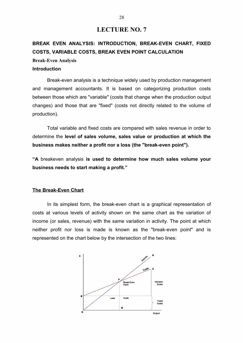
The Break-Even Chart
In its simplest form, the break-even chart is a graphical representation of
costs at various levels of activity shown on the same chart as the variation of
income (or sales, revenue) with the same variation in activity. The point at which
neither profit nor loss is made is known as the "break-even point" and is
represented on the chart below by the intersection of the two lines:
28
In the diagram above, the line OA represents the variation of income at
varying levels of production activity ("output"). OB represents the total fixed costs
in the business. As output increases, variable costs are incurred, meaning that
total costs (fixed + variable) also increase. At low levels of output, Costs are
greater than Income. At the point of intersection, P, costs are exactly equal to
income, and hence neither profit nor loss is made.
Fixed Costs
Fixed costs are those business costs that are not directly related to the
level of production or output. In other words, even if the business has a zero
output or high output, the level of fixed costs will remain broadly the same. In the
long term fixed costs can alter - perhaps as a result of investment in production
capacity (e.g. adding a new factory unit) or through the growth in overheads
required to support a larger, more complex business.
Examples of fixed costs:
- Rent and rates
- Depreciation
- Research and development
- Marketing costs (non- revenue related)
- Administration costs
Variable Costs
Variable costs are those costs which vary directly with the level of output.
They represent payment output-related inputs such as raw materials, direct
labour, fuel and revenue-related costs such as commission.
Break Even Point Calculation
Calculation of BEP can be done using the following formula :
)( VCUPSUP
TFCBEP
−=
where ,
BEP = break-even point (Units of production)
TFC = total fixed costs
29
VCUP = variable costs per unit of production
SUP = Selling price per unit of production
For example, suppose that fixed costs for producing 100,000 widgets were
$30,000 a year. Variable costs are $2.20 materials, $4.00 labour, and $0.80
overhead, for a total of $7.00. If selling price was chosen as $12.00 for each
widget, then: Break even point will be $30,000 divided by ($12.00 - 7.00) equals
6000 units.This is the number of widgets that have to be sold at a selling price of
$12.00 before business will start to make a profit.
Advantages of Break Even Analysis
It explains the relationship between cost, production volume and returns.
The major benefit to using break-even analysis is that it indicates the lowest
amount of business activity necessary to prevent losses.
Limitations of Break-even -Analysis
It is best suited to the analysis of one product at a time
30
LECTURE NO. 8
PLANT LOCATION: INTRODUCTION, LOCATION DECISION PROCESS,
FACTORS INVOLVED IN THE PLANT LOCATION DECISION
Introduction
Plant location decisions are strategic, long term and non-repetitive in
nature. Without sound and careful location planning in the beginning itself, the
new plant may pose continuous operating disadvantages. Location decisions are
affected by many factors, both internal and external to the organization’s
operations.
Internal factors include the technology used, the capacity, the financial
position, and the work force required.
External factors include the economic, political and social conditions in the
various localities.
Most of the fixed and some of the variable costs are determined by the
location decision. The efficiency, effectiveness, productivity and profitability of the
plant are also affected by the location decision. Location decisions are based on a
host of factors, some subjective, qualitative and intangible while some others are
objective, quantitative and tangible.
When Does a Location Decision Arise?
The impetus to embark upon a plant location study can be attributed to
reasons as given below:
• It may arise when a new plant is to be established.
• In some cases, the plant operations and subsequent expansion are
restricted by a poor site, thereby necessitating the setting up of the facility
at a new site.
• The growing volume of business makes it advisable to establish additional
facilities in new territories.
• Decentralization and dispersal of industries reflected in the industrial policy
resolution so as to achieve an overall development would necessitate a
location decision at a macro level.
• It could happen that the original advantages of the plant have been
outweighed due to new developments.
• New economic, social, legal or political factors could suggest a change of
location of the existing plant.
31
Some or all the above factors could force a firm or an organization to
question whether the location of its plant should be changed or not.
Whenever the plant location decision arises, it deserves careful attention
because of the long-term consequences. Any mistake in selection of a proper
location could prove to be costly. Poor location could be a constant source of
higher cost, higher investment, difficult marketing and transportation, dissatisfied
and frustrated employees and consumers, frequent interruptions of production,
abnormal wastage, delays and substandard quality, denied advantages of
geographical specialization and so on. Once a plant is set up at a location, it is
very difficult to shift later to a better location because of numerous economic,
political and sociological reasons.
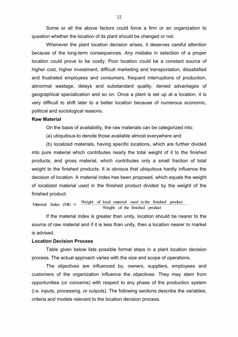
Raw Material
On the basis of availability, the raw materials can be categorized into:
(a) ubiquitous-to denote those available almost everywhere and
(b) localized materials, having specific locations, which are further divided
into pure material which contributes nearly the total weight of it to the finished
products, and gross material, which contributes only a small fraction of total
weight to the finished products. It is obvious that ubiquitous hardly influence the
decision of location. A material index has been proposed, which equals the weight
of localized material used in the finished product divided by the weight of the
finished product.
product finished theofWeight product finished in the used material local ofWeight
(MI)Index Material =
If the material index is greater than unity, location should be nearer to the
source of raw material and if it is less than unity, then a location nearer to market
is advised.
Location Decision Process
Table given below lists possible formal steps in a plant location decision
process. The actual approach varies with the size and scope of operations.
The objectives are influenced by, owners, suppliers, employees and
customers of the organization influence the objectives. They may stem from
opportunities (or concerns) with respect to any phase of the production system
(i.e. inputs, processing, or outputs). The following sections describe the variables,
criteria and models relevant to the location decision process.
32
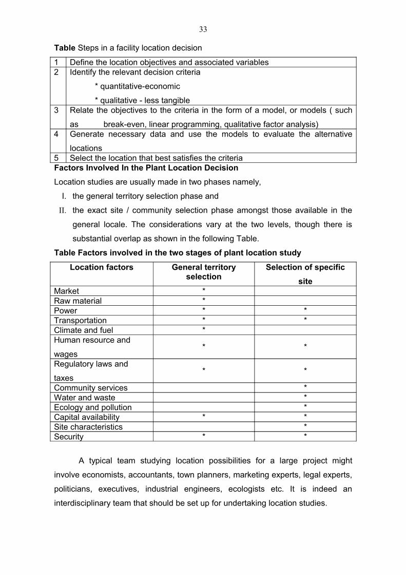
Table Steps in a facility location decision
1 Define the location objectives and associated variables2 Identify the relevant decision criteria
* quantitative-economic
* qualitative - less tangible3 Relate the objectives to the criteria in the form of a model, or models ( such
as break-even, linear programming, qualitative factor analysis) 4 Generate necessary data and use the models to evaluate the alternative
locations5 Select the location that best satisfies the criteriaFactors Involved In the Plant Location Decision
Location studies are usually made in two phases namely,
I. the general territory selection phase and
II. the exact site / community selection phase amongst those available in the
general locale. The considerations vary at the two levels, though there is
substantial overlap as shown in the following Table.
Table Factors involved in the two stages of plant location study
Location factors General territory selection
Selection of specific
siteMarket *Raw material *Power * *Transportation * *Climate and fuel *Human resource and
wages* *
Regulatory laws and
taxes* *
Community services *Water and waste *Ecology and pollution *Capital availability * *Site characteristics *Security * *
A typical team studying location possibilities for a large project might
involve economists, accountants, town planners, marketing experts, legal experts,
politicians, executives, industrial engineers, ecologists etc. It is indeed an
interdisciplinary team that should be set up for undertaking location studies.
33
LECTURE NO. 9TERRITORY SELECTION AND SITE/ COMMUNITY SELECTION
Territory Selection
For the general territory / region / area, the following are some of the
important factors that influence the selection decision.
1. Markets: There has to be some customer / market for the product. The market
growth potential and the location of competitors are important factors that could
influence the location. Locating a plant or facility nearer to the market is preferred
if promptness of service is required particularly if the product is susceptible to
spoilage. Also if the product is relatively inexpensive and transportation costs add
substantially to the cost, a location close to the market is desirable.
2. Raw materials and supplies: Sometimes accessibility to vendors/suppliers of
raw materials, equipment etc. may be very important. The issue here is
promptness and regularity of delivery and inward freight cost minimization.
If the raw material is bulky or low in cost, or if it is greatly reduced in bulk
viz. transformed into various products and by-products or if it is perishable and
processing makes it less so, then location near raw material source is important. If
raw materials come from a variety of locations, the plant / facility may be situated
so as to minimize total transportation costs. The costs vary depending upon
specific routes, mode of transportation and specific product classifications
3. Transportation facilities: Adequate transportation facilities are essential for
the economic operation of production system. For companies that produce or buy
heavy bulky and low value per ton commodities, water transportation could be an
important factor in location plants.
4. Manpower supply: The availability of skilled manpower, the prevailing wage
pattern, living costs and the industrial relations situation influence the location.
5. Infrastructure: This factor refers to the availability and reliability of power,
water, fuel and communication facilities in addition to transportation facilities.
6. Legislation and taxation: Factors such as financial and other incentives for
new industries in backward areas or no-industry-district centers, exemption from
certain state and local taxes, octroi etc. are important.
Site / Community Selection
Having selected the general territory / region, one would have to go in for
site / community selection. Some factors relevant for this are:
34
1. Community facilities: These involve factors such as quality of life which in
turn depends on availability of facilities like education, places of worship, medical
services, police and fire stations, cultural, social and recreation opportunities,
housing, good streets and good communication and transportation facilities.
2. Community attitudes: These can be difficult to evaluate. Most communities
usually welcome setting up of a new industry especially since it would provide
employment opportunities to the local people directly or indirectly. However, in
case of polluting industries, they would try their utmost to locate them as far away
as possible. Sometimes because of prevailing law and order situation, companies
have been forced to relocate their units. The attitude of people as well as the state
government has an impact on location of polluting and hazardous industries.
3. Waste disposal: The facilities required for the disposal of process waste
including solid, liquid and gaseous effluent need to be considered. The plant
should be positioned so that prevailing winds carry any fumes away from
populated areas and that the waste may be disposed off properly and at
reasonable costs.
4. Ecology and pollution: These days, there is a great deal of awareness
towards maintenance of natural ecological balance. There are quite a few
agencies propagating the concepts to make the society at large more conscious
of the dangers of certain available actions.
5. Site size: The plot of land must be large enough to hold the proposed plant and
parking and access facilities and provide room for future expansion.
6. Topography: -The topography, soil structure and drainage must be suitable. If
considerable land improvement is required, low priced land might turn out to be
expensive.
7. Transportation facilities: The site should be accessible preferably by road
and rail. The dependability and character of the available transport carriers,
frequency of service and freight and terminal facilities is also worth considering.
8. Supporting industries and services: The availability of supporting services
such as tool rooms, plant services etc. need to be considered.
9. Land costs: These are generally of lesser importance, as they are non-
recurring and possibly make up a relatively small proportion of the total cost of
locating a new plant.
Generally, the site will be in a city, suburb or country location. In general,
the location for large scale industries should be in rural areas, which helps in
35
regional development also. It is seen that once a large industry is set up (or even
if a decision to this effect has been taken), a lot of infrastructure develops around
it as a result of the location decision. As for the location of medium scale
industries is concerned, these could be preferably in the suburban / semi-urban
areas where the advantages of urban and rural areas are available. For the small-
scale industries, the location could be urban areas where the infrastructural
facilities are already available. However, in real life, the situation is somewhat
paradoxical as people, with money and means, are usually in the cities and would
like to locate the units in the city itself.
Some of the industrial needs and characteristics that tend to favour each of
this location are.
Requirements governing choice of a city location are:
• Availability of adequate supply of labour force
• High proportion of skilled employees
• Rapid public transportation and contact with suppliers and
customers
• Small plant site or multi floor operation
• Processes heavily dependent on city facilities and utilities
• Good communication facilities like telephone, telex, post
offices
• Good banking and health care delivery systems
Requirements governing the choice of a suburban location are:
• Large plant site close to transportation or population centre
• Free from some common city building zoning (industrial
areas) and other restrictions
• Freedom from higher parking and other city taxes etc.
• Labour force required to reside close to the plant
• Community close to, but not in large population centre
• Plant expansion easier than in the city
Requirements governing the choice of a rural location are:
• Large plant site required for either present demands or
expansion
• Dangerous production processes
• Lesser effort required for anti-pollution measures
36
• Large volume of relatively clean water
• Lower property taxes, away from Urban Land Ceiling Act
restrictions
• Protection against possible sabotage or for a secret process
• Balanced growth and development of a developing or
underdeveloped area
• Unskilled labour force required
• Low wages required to meet competition
37
LECTURE NO. 10
SUBJECTIVE, QUALITATIVE AND SEMI-QUANTITATIVE TECHNIQUES,
EQUAL WEIGHTS METHOD, VARIABLE WEIGHTS METHOD, WEIGHT-CUM-
RATING METHOD, ANOTHER WEIGHT-CUM-RATING METHOD
Subjective, Qualitative and Semi-Quantitative Techniques
Three subjective techniques used for facility location are Industry
Precedence, Preferential Factor and Dominant Factor. In the industry precedence
subjective technique, the basic assumption is that if a location was best for similar
firms in the past, it must be the best for the new one now. As such, there is no
need for conducting a detailed location study and the location choice is thus
subject to the principle of precedence - good or bad.
However, in the case of the preferential factor, the location decision is
dictated by a personal factor. It depends on the individual whims or preferences
e.g. if one belongs to a particular state, he / she may like to locate his / her unit
only in that state. Such personal factors may override factors of cost or profit in
taking a final decision. This could hardly be called a professional approach though
such methods are probably more common in practice than generally recognized.
However, in some cases of plant location there could be a certain dominant
factor (in contrast to the preferential factor) which could influence the location
decision. In a true dominant sense, mining or petroleum drilling operations must
be located where the mineral resource is available. The decision in this case is
simply whether to locate or not at the source.
For evaluating qualitative factors, some factor ranking and factor weight
rating systems may be used. In the ranking procedure, a location is better or
worse than another for the particular factor. By weighing factors and rating
locations against these weights a semi-quantitative comparison of location is
possible. Let us now discuss some specific methods.
Equal Weights Method
Assign equal weights to all factors and evaluate each location along the
factor scale. For example, a manufacturer of fabricated foods selected three
factors by which to rate four sites. Each site was assigned a rating of 0 to 10
points for each factor. The sum of the assigned factor points constituted the site
rating by which it could be compared to other site.
38
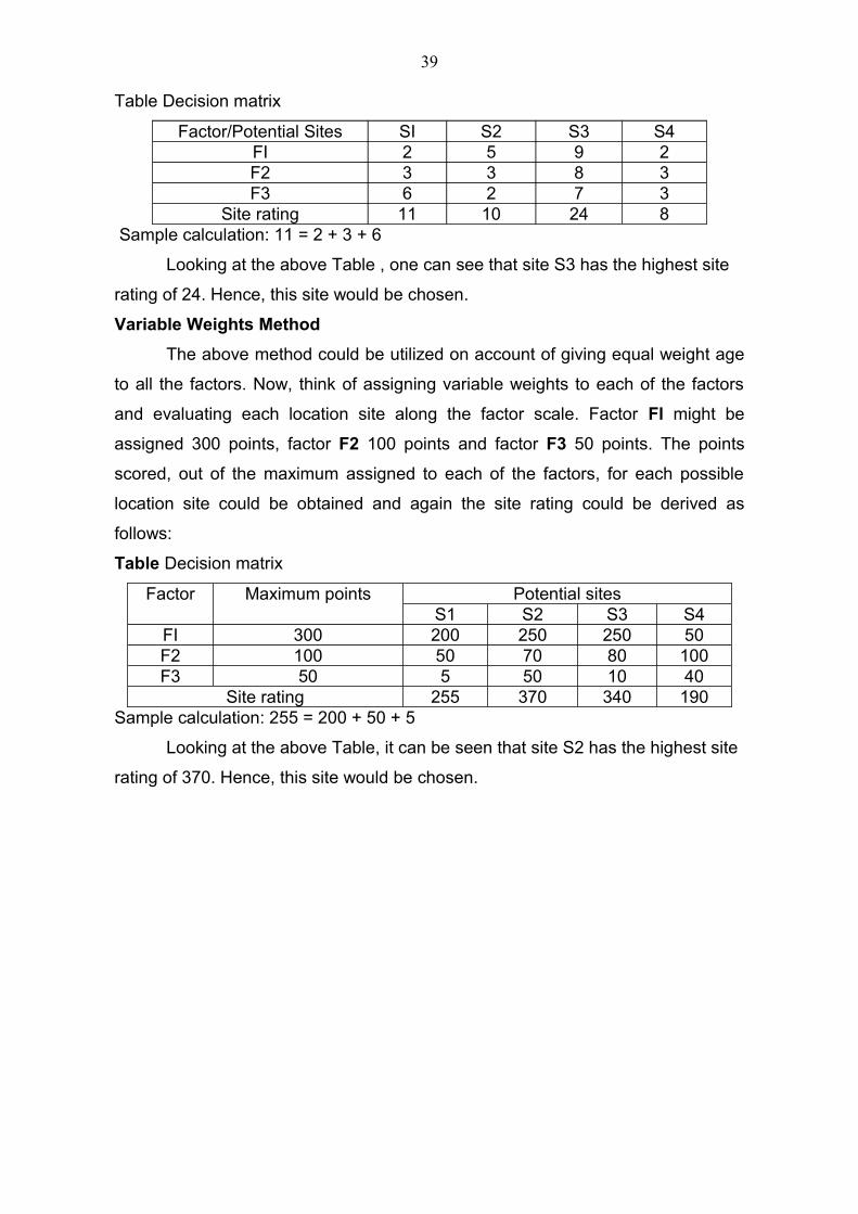
Table Decision matrix
Factor/Potential Sites SI S2 S3 S4FI 2 5 9 2F2 3 3 8 3F3 6 2 7 3
Site rating 11 10 24 8 Sample calculation: 11 = 2 + 3 + 6
Looking at the above Table , one can see that site S3 has the highest site
rating of 24. Hence, this site would be chosen.
Variable Weights Method
The above method could be utilized on account of giving equal weight age
to all the factors. Now, think of assigning variable weights to each of the factors
and evaluating each location site along the factor scale. Factor Fl might be
assigned 300 points, factor F2 100 points and factor F3 50 points. The points
scored, out of the maximum assigned to each of the factors, for each possible
location site could be obtained and again the site rating could be derived as
follows:
Table Decision matrix
Factor Maximum points Potential sitesS1 S2 S3 S4
FI 300 200 250 250 50F2 100 50 70 80 100F3 50 5 50 10 40
Site rating 255 370 340 190Sample calculation: 255 = 200 + 50 + 5
Looking at the above Table, it can be seen that site S2 has the highest site
rating of 370. Hence, this site would be chosen.
39
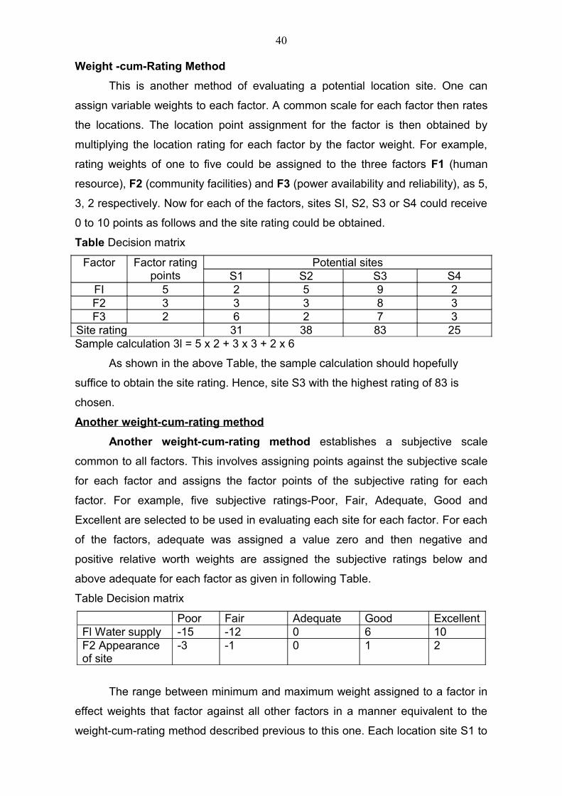
Weight -cum-Rating Method
This is another method of evaluating a potential location site. One can
assign variable weights to each factor. A common scale for each factor then rates
the locations. The location point assignment for the factor is then obtained by
multiplying the location rating for each factor by the factor weight. For example,
rating weights of one to five could be assigned to the three factors F1 (human
resource), F2 (community facilities) and F3 (power availability and reliability), as 5,
3, 2 respectively. Now for each of the factors, sites SI, S2, S3 or S4 could receive
0 to 10 points as follows and the site rating could be obtained.
Table Decision matrix
Factor Factor rating points
Potential sitesS1 S2 S3 S4
FI 5 2 5 9 2F2 3 3 3 8 3F3 2 6 2 7 3
Site rating 31 38 83 25Sample calculation 3l = 5 x 2 + 3 x 3 + 2 x 6
As shown in the above Table, the sample calculation should hopefully
suffice to obtain the site rating. Hence, site S3 with the highest rating of 83 is
chosen.
Another weight-cum-rating method
Another weight-cum-rating method establishes a subjective scale
common to all factors. This involves assigning points against the subjective scale
for each factor and assigns the factor points of the subjective rating for each
factor. For example, five subjective ratings-Poor, Fair, Adequate, Good and
Excellent are selected to be used in evaluating each site for each factor. For each
of the factors, adequate was assigned a value zero and then negative and
positive relative worth weights are assigned the subjective ratings below and
above adequate for each factor as given in following Table.
Table Decision matrix
Poor Fair Adequate Good ExcellentFl Water supply -15 -12 0 6 10F2 Appearance of site
-3 -1 0 1 2
The range between minimum and maximum weight assigned to a factor in
effect weights that factor against all other factors in a manner equivalent to the
weight-cum-rating method described previous to this one. Each location site S1 to
40
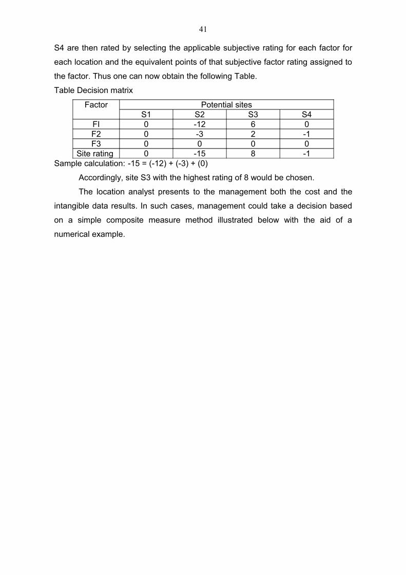
S4 are then rated by selecting the applicable subjective rating for each factor for
each location and the equivalent points of that subjective factor rating assigned to
the factor. Thus one can now obtain the following Table.
Table Decision matrix
Factor Potential sitesS1 S2 S3 S4
FI 0 -12 6 0F2 0 -3 2 -1F3 0 0 0 0
Site rating 0 -15 8 -1Sample calculation: -15 = (-12) + (-3) + (0)
Accordingly, site S3 with the highest rating of 8 would be chosen.
The location analyst presents to the management both the cost and the
intangible data results. In such cases, management could take a decision based
on a simple composite measure method illustrated below with the aid of a
numerical example.
41
LECTURE NO. 11
COMPOSITE MEASURE METHOD, LOCATIONAL BREAK-EVEN ANALYSIS
Composite Measure Method
The steps of the composite measure method are:
• Develop a list of all relevant factors
• Assign a scale to each factor and designate some minimum
• Weigh the factors relative to each other in light of importance towards
achievement of system goals. .
• Score each potential location according to the designated scale and
multiply the scores by the weights.
• Total the points each location and either (a) use them in conjunction with a
separate economic analysis, or (b) include an economic factors in the list of
factors and choose the location on the basis of maximum points.
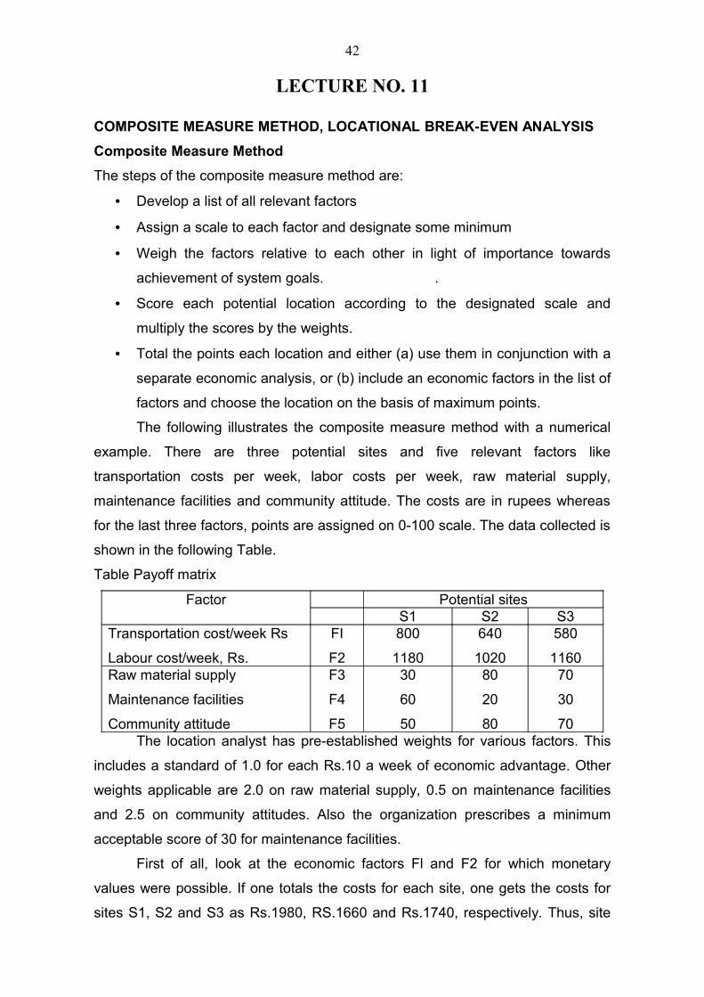
The following illustrates the composite measure method with a numerical
example. There are three potential sites and five relevant factors like
transportation costs per week, labor costs per week, raw material supply,
maintenance facilities and community attitude. The costs are in rupees whereas
for the last three factors, points are assigned on 0-100 scale. The data collected is
shown in the following Table.
Table Payoff matrix
Factor Potential sitesS1 S2 S3
Transportation cost/week Rs
Labour cost/week, Rs.
FI
F2
800
1180
640
1020
580
1160Raw material supply
Maintenance facilities
Community attitude
F3
F4
F5
30
60
50
80
20
80
70
30
70The location analyst has pre-established weights for various factors. This
includes a standard of 1.0 for each Rs.10 a week of economic advantage. Other
weights applicable are 2.0 on raw material supply, 0.5 on maintenance facilities
and 2.5 on community attitudes. Also the organization prescribes a minimum
acceptable score of 30 for maintenance facilities.
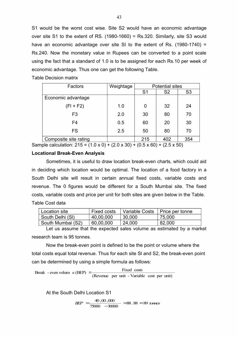
First of all, look at the economic factors Fl and F2 for which monetary
values were possible. If one totals the costs for each site, one gets the costs for
sites S1, S2 and S3 as Rs.1980, RS.1660 and Rs.1740, respectively. Thus, site
42
S1 would be the worst cost wise. Site S2 would have an economic advantage
over site S1 to the extent of RS. (1980-1660) = Rs.320. Similarly, site S3 would
have an economic advantage over site SI to the extent of Rs. (1980-1740) =
Rs.240. Now the monetary value in Rupees can be converted to a point scale
using the fact that a standard of 1.0 is to be assigned for each Rs.10 per week of
economic advantage. Thus one can get the following Table.
Table Decision matrix
Factors Weightage Potential sitesS1 S2 S3
Economic advantage
(Fl + F2)
F3
F4
FS
1.0
2.0
0.5
2.5
0
30
60
50
32
80
20
80
24
70
30
70
Composite site rating 215 402 354Sample calculation: 215 = (1.0 x 0) + (2.0 x 30) + (0.5 x 60) + (2.5 x 50)
Locational Break-Even Analysis
Sometimes, it is useful to draw location break-even charts, which could aid
in deciding which location would be optimal. The location of a food factory in a
South Delhi site will result in certain annual fixed costs, variable costs and
revenue. The 0 figures would be different for a South Mumbai site. The fixed
costs, variable costs and price per unit for both sites are given below in the Table.
Table Cost data
Location site Fixed costs Variable Costs Price per tonne South Delhi (Sl) 40,00,000 30,000 75,000 South Mumbai (S2) 60,00,000 24,000 82,000
Let us assume that the expected sales volume as estimated by a market
research team is 95 tonnes.
Now the break-even point is defined to be the point or volume where the
total costs equal total revenue. Thus for each site Sl and S2, the break-even point
can be determined by using a simple formula as follows:
unit)per cost Variable -unitper (Revenue
costs Fixed (BEP) eeven volum-Break =
At the South Delhi Location S1
tonnesBEP 8988.883000075000
000,00,40 ==−
=
43
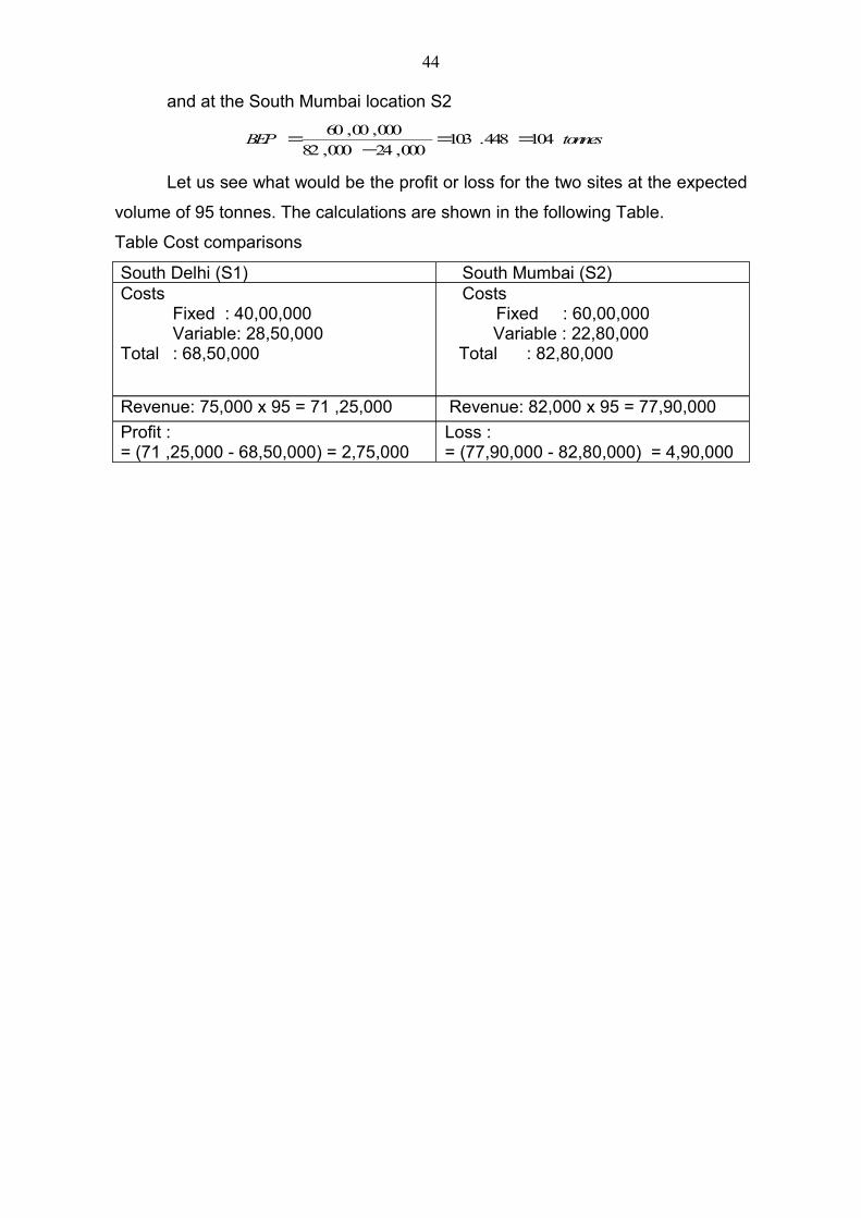
and at the South Mumbai location S2
tonnesBEP 104448.103000,24000,82
000,00,60 ==−
=
Let us see what would be the profit or loss for the two sites at the expected
volume of 95 tonnes. The calculations are shown in the following Table.
Table Cost comparisons
South Delhi (S1) South Mumbai (S2) Costs
Fixed : 40,00,000Variable: 28,50,000
Total : 68,50,000
CostsFixed : 60,00,000
Variable : 22,80,000 Total : 82,80,000
Revenue: 75,000 x 95 = 71 ,25,000 Revenue: 82,000 x 95 = 77,90,000
Profit := (71 ,25,000 - 68,50,000) = 2,75,000
Loss : = (77,90,000 - 82,80,000) = 4,90,000
44
LECTURE NO. 12
FOOD PLANT UTILITIES: PROCESS WATER, STEAM, ELECTRICITY, PLANT
EFFLUENTS
FOOD PLANT UTILITIES
The principal plant utilities in a food plant are process water, process
steam, electric power for motors and lighting, and fuel.
Process Water
Process water is required for washing the raw materials and for various
cooling operations. In fruit and vegetable processing plants, water may be used
for transportation (fluming) of the raw materials from receiving to processing
areas. Water used in steam boilers may require ion exchange treatment to reduce
its hardness. Total water requirement in fruit and vegetable processing may range
from 5 to 15 m3 / ton of raw material.
2. Steam
Steam boilers are needed in most food processing plants to provide
process steam, used mainly in various operations, such as heating of process
vessels, evaporators and dryers, sterilization, blanching, and peeling. A medium
size food plant (80 tons / day raw material) may require a boiler producing about
10 tons/h of steam at 18 bar pressure.
Two principal types of steam boilers are used in the food processing
industry, i.e. the fire-tube and the water-tube boilers. The fire tube boilers operate
at relatively lower pressure (1–24 bar) and produce cleaner steam. The water-
tube units operate at higher pressures (100–140 bar) and they are suited for co-
generation, i.e. electrical power and exhaust steam of lower pressure for process
heating. Co-generation is economical in large food plants, requiring large amounts
of low-pressure steam, e.g., beet sugar plants.
A standby steam boiler of proper capacity may be necessary to provide
process steam during any boiler failure or breakdown.
Steam boilers are rated in Btu/h, kW or boiler HP (1 Btu/h = 0.293 W, 1
boiler HP = 9.8 kW). The heat flux in the boiler heating surface is about 0.75 k W/
m2. The boiler efficiency is about 85% with most of the thermal losses in the dry
gases and the moisture. Steam generation is about 1.4 t/h per MW.
45
In order to maintain the concentration of accumulated dissolved solids in
steam boilers below 3500 ppm, periodic discharge of hot water (blow down) is
practiced.
Fuel is used in food plants mostly for generating process steam and
process drying. Natural gas and liquefied propane (LPG) are preferred fuels in
food processing, because their combustion gases are not objectionable in direct
contact with food products. Fuel oil and coal can be used for indirect heating, i.e.
through heat exchangers.
Culinary steam of special quality is used when steam is injected in food
products. The steam must be free of objectionable chemicals used in boilers,
which may be carried into the food being heated. Culinary steam is usually
produced from potable water in a secondary system of a heat exchanger heated
with high pressure industrial steam.
3. Electricity
Electrical power in food processing plants is needed for running the motors
of the processing, control, and service equipment, for industrial heating, and for
illumination. For a medium size food plant processing about 100 tons/day raw
materials, the power requirement may of the order of 500 kW. A standby power
generator of about 200 k VA is recommended for emergency operation of the
main plant, in case of power failure or breakdown.
Single-phase or three-phase alternating current (AC) of 110 V (60 cycles)
or 220 V (50 cycles) is used in food processing plants. The electrical motors are
either single-phase or three-phase squirrel cage.
Energy-efficient electrical motors should be used in various food
processing operations. A measure of the efficiency of electrical power is the
power factor (pf), defined as pf = VAk
Wk , which should be equal or higher than
0.85.
Illuminating (lighting) of industrial food plants should utilize fluorescent
lamps, which can save significant amounts of energy.
4. Plant Effluents
46
Plant effluents consisting mainly of wastewater, but including solids and
gas wastes require special handling and treatments to comply with the local laws
and regulations.
Food plants should be designed and operated so that a minimum pollution
is caused to the environment. The Environmental Protection Agency (EPA) in the
US has issued codes and regulations that ensure the quality of natural water
bodies is not damaged by effluent discharges from industrial plants. Similar
regulations apply to atmospheric emissions of objectionable gases and dust.
Environmental information needed to comply with EPA regulations for wastewater
includes testing for pH, temperature, biochemical oxygen demand (BOD), fats oil
and grease (FOG), and total suspended solids (TSS).
Large amounts of waste are produced in the processing of fruits and
vegetables, as in canning, freezing, and dehydration operations. Smaller waste
volumes are produced in dairy plants (with the exception of cheese and milk
powder), and in dry-processing (milling) of grain (e.g., wheat flour).
A medium size fruit or vegetable processing plant handling about 100
ton/day of raw materials may discharge about 1000 m3/day of waste water.
Treatment of food waste water may involve one or more of the following
operations:
1. Simple screening out of the suspended solids,
2. Gravel filtration,
3. solids settling in sedimentation tanks,
4. biological oxidation (aeration),
5. spray irrigation,
6. discharge into the local public sewer, and
7. discharge into a waterway.
Liquid wastes (waste water) can be disposed to the local waste (sewage)
treatment plants, after removing some objectionable components, such as fat, oil,
and grease to an acceptable level, e.g., lower than 1000 mg/L. Pollution loads
higher than 200 mg/L are common in food plant liquid wastes. It is more
economical to pay pollution surcharges to the local sewage plant, whenever
possible, than to build an expensive wastewater treatment facility.
Food preservation plants, located away from municipal sewage systems,
dispose the process water to large storage ponds (lagoons), where a slow natural
47
bio-oxidation of the organic waste takes place. The treated lagoon wastewater
can be discharged to the land adjoining the plants.
Some solid food wastes can be sold at relatively low prices for animal
feeds, either unprocessed or dried, e.g., solid citrus or sugar beet wastes. Some
solid food wastes can be diverted to the land (grape pomace to vineyard), while
some other can be mixed with the soil (composting).
The sanitary sewage of food plants, depending on the number of
employees, should be treated in a different system than the process wastewater.
It can be discharged to the local sewage system, if available. Otherwise, it is
treated in septic tanks constructed near the food plant.
Relatively small amounts of gas wastes (odorous VOC) are generated by
some food industries, such as bakeries (ethanol), fishmeal dryers, and edible oil
refining plants. Also, odors from coffee and cocoa roasting may require some form
of treatment. Treatment of objectionable gas wastes involves gas absorption
equipment, such as wet scrubbers.
The design of treatment facilities for industrial wastewater, and solids/gas
wastes requires the expertise of environmental engineers who are familiar with
the local laws and regulations concerning environmental pollution.
48
LECTURE NO. 13
PLANT SIZE AND FACTORS
Plant size / capacity for any food-processing unit refers to the planned rate
of production of the identified product(s). It can be expressed in terms of either
volume or weight or number produced per unit time of the product. The time
unit for expressing the plant size could be taken as hour or a shift or a day or a
year. It is always useful to take a decision about the size/capacity in the beginning
of the plant design.
Knowledge of the plant size may help in:
• assessing the type and size of the plant and machinery needed
• assessing the size and caliber of the work force needed
• determining the requirements of total land area and covered space for
the plant
• deciding the type of layout
• assessing the other physical facilities needed
• determining the type of sales efforts and distribution system
• financial or economic viability calculations
The size/capacity of the plant will depend on a number of factors such as:
• raw material availability :
• market demand
• degree and nature of the market competition
• economic considerations i.e. acceptable return on investment /
profitability
The interaction of each of the above factor with plant size can be assessed
on the basis of information collected as part of the market study. Therefore, a
comprehensive market study is a must.
Raw Material Availability
There may be adequate or unlimited demand for the product in the market
with little or no competition, but the entrepreneur may not get adequate supplies
of the raw material to produce the product in quantities one wishes. This would
limit the size.
Market Demand
Market demand for any product is the total volume that will be bought by a
defined customer group in defined geographical area in a defined time period
49
and in a defined environment. It is possible that the raw material is available in
abundance. One can get as much raw material as one wishes. But one can not
sell all that one can produce. The demand for the product is limited. In this
case, it is the market demand, which will determine the plant size.
Degree and Nature of the Market Competition
There is no restriction on raw material availability. It is available in
abundance. Also, there is enough demand for the product in the market.
However, there exist a large number of manufacturers / processors for the
product who are expected to provide stiff competition. In this case, the plant size
may be restricted to a limit governed by the share of the market, which the
entrepreneur may capture. Depending on the product, a 10 - 15% market share is
considered to be adequate. The competition may involve price or quality or timely
delivery or a combination of such features. To study the competition, the
entrepreneur needs to have a list of major competitors, details of their product
range, product features, output, market share and pricing.
Economic Considerations
Many times plant size is determined by the financial resources available
with the entrepreneur as also by the degree of risk the entrepreneur is prepared to
take. Sometimes it is also advisable to find the popular plant size of existing
enterprises engaged in manufacturing/processing the product of choice.
In cases where the availability of raw material, market demand and the
financial resources are not a problem, the entrepreneur may look for the size
which will ensure him / her a minimum acceptable return/profit. This size is
called the minimum economically viable plant size. However, when situation
permits a plant size larger than the minimum economically viable size, a size,
which will maximize profits, is selected.
The minimum acceptable return/profit viewed in two ways. In one case
larger share of the capital investment may consist of the equity (entrepreneur's
own capital) while in another case it may consist of the borrowed capital. In case
of the former, the return/profit must be greater than the amount of interest earned
if the entire capital of the entrepreneur was invested as fixed deposit in a
scheduled bank. In case of the later, the return/profit must be greater than the
interest paid on the borrowed capital.
While deciding the plant size/capacity one should also remember the
following:
50

• Specify the number of days for which the proposed plant will work in a
year. In general, it is customary to presume 300 working days. However, if
the enterprise is to handle the seasonal product, it may work for less than
300 days.
• One shift consists of 8 hours. One shift working is the most popular pattern
among small enterprises. Two and three shift working is largely limited to
continuous enterprises and the medium and large-scale enterprises.
51
LECTURE NO. 14
THE ENTERPRISE AND ITS ENVIRONMENT, THE TOTAL REVENUE
FUNCTION, THE TOTAL COST FUNCTION
The Enterprise and Its Environment
Imagine a food processing enterprise that competes with several others.
The enterprise produces a single product, has some control over the price it will
charge and is primarily devoted to making a profit. Imagine further that the major
characteristics of the market, the competitors, and enterprises own internal
technology are well known to management and essentially static in time. Under
these conditions one may explore some of the major economic decisions that
might be made. One may start with the environment in which the enterprise exists
and work inward, eventually reaching the level of decisions at which the analyst
often works.
In studying the enterprise's environment one might wish to study in detail
the customers, competitors, suppliers, and the legal, political, social and
geographic factors which bear upon its operations. To avoid some of the chaos
this might involve, it is assumed that all these things can be expressed by the
demand curve of the enterprise. The demand curve expresses a part of the
relationship of the enterprise with its market by simply giving the amount of
product that can be sold as a function of the price charged for it. In this simple
model, price is taken to be the major determining factor in the amount the
enterprise can sell; and such obvious other factors as quality, advertising, sales
effort, reputation, and service are left out of the picture. Thus the relationship
between the price and the amount of product that can be sold is given by:
P = a – b D for 0 ≤ D ≤ a/b
= 0 otherwise
Here P is the unit price, D is the amount of product sold, and a and b are
positive constants. It is assumed that the amount of product, D, is a continuous
variable. The straight-line example, which has been given, might have been a
curve; but the point is that one usually expects large volume to be associated with
low price, and small volume to be associated with high price (Figure 1).
The analyst who knows the demand curve may then decide what price one
will charge, and the curve will tell how much one can sell; or, one may decide
52
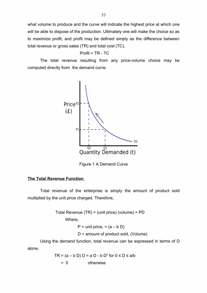
what volume to produce and the curve will indicate the highest price at which one
will be able to dispose of the production. Ultimately one will make the choice so as
to maximize profit, and profit may be defined simply as the difference between
total revenue or gross sales (TR) and total cost (TC),
Profit = TR - TC
The total revenue resulting from any price-volume choice may be
computed directly from the demand curve.
Figure 1 A Demand Curve
The Total Revenue Function
Total revenue of the enterprise is simply the amount of product sold
multiplied by the unit price charged. Therefore,
Total Revenue (TR) = (unit price) (volume) = PD
Where,
P = unit price, = (a – b D)
D = amount of product sold, (Volume)
Using the demand function, total revenue can be expressed in terms of D
alone,
TR = (a – b D) D = a D - b D2 for 0 ≤ D ≤ a/b
= 0 otherwise
53
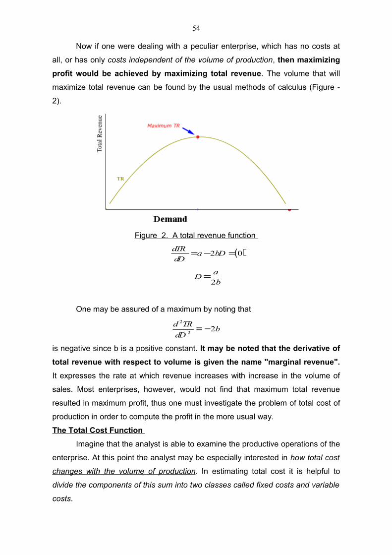
Now if one were dealing with a peculiar enterprise, which has no costs at
all, or has only costs independent of the volume of production, then maximizing
profit would be achieved by maximizing total revenue. The volume that will
maximize total revenue can be found by the usual methods of calculus (Figure -
2).
Figure 2. A total revenue function
( )02 =−= bDadD
dTR
b
aD
2=
One may be assured of a maximum by noting that
bdD
TRd2
2
2
−=
is negative since b is a positive constant. It may be noted that the derivative of
total revenue with respect to volume is given the name "marginal revenue".
It expresses the rate at which revenue increases with increase in the volume of
sales. Most enterprises, however, would not find that maximum total revenue
resulted in maximum profit, thus one must investigate the problem of total cost of
production in order to compute the profit in the more usual way.
The Total Cost Function
Imagine that the analyst is able to examine the productive operations of the
enterprise. At this point the analyst may be especially interested in how total cost
changes with the volume of production. In estimating total cost it is helpful to
divide the components of this sum into two classes called fixed costs and variable
costs.
54
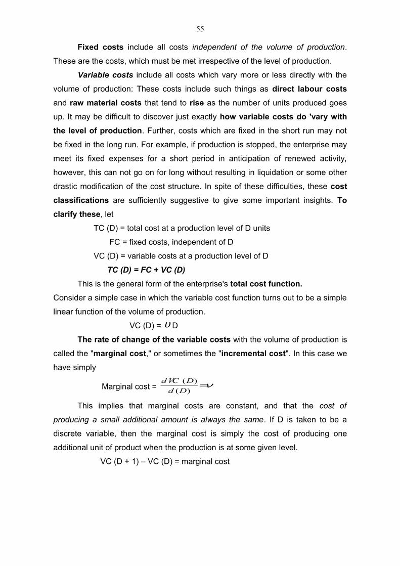
Fixed costs include all costs independent of the volume of production.
These are the costs, which must be met irrespective of the level of production.
Variable costs include all costs which vary more or less directly with the
volume of production: These costs include such things as direct labour costs
and raw material costs that tend to rise as the number of units produced goes
up. It may be difficult to discover just exactly how variable costs do 'vary with
the level of production. Further, costs which are fixed in the short run may not
be fixed in the long run. For example, if production is stopped, the enterprise may
meet its fixed expenses for a short period in anticipation of renewed activity,
however, this can not go on for long without resulting in liquidation or some other
drastic modification of the cost structure. In spite of these difficulties, these cost
classifications are sufficiently suggestive to give some important insights. To
clarify these, let
TC (D) = total cost at a production level of D units
FC = fixed costs, independent of D
VC (D) = variable costs at a production level of D
TC (D) = FC + VC (D)
This is the general form of the enterprise's total cost function.
Consider a simple case in which the variable cost function turns out to be a simple
linear function of the volume of production.
VC (D) = υ D
The rate of change of the variable costs with the volume of production is
called the "marginal cost," or sometimes the "incremental cost". In this case we
have simply
Marginal cost = ν=)(
)(
Dd
DVCd
This implies that marginal costs are constant, and that the cost of
producing a small additional amount is always the same. If D is taken to be a
discrete variable, then the marginal cost is simply the cost of producing one
additional unit of product when the production is at some given level.
VC (D + 1) – VC (D) = marginal cost
55
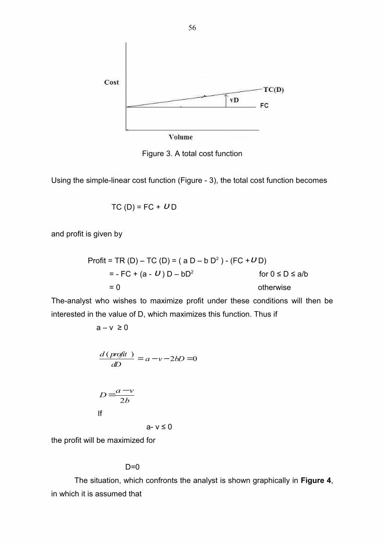
Figure 3. A total cost function
Using the simple-linear cost function (Figure - 3), the total cost function becomes
TC (D) = FC + υ D
and profit is given by
Profit = TR (D) – TC (D) = ( a D – b D2 ) - (FC +υ D)
= - FC + (a - υ ) D – bD2 for 0 ≤ D ≤ a/b
= 0 otherwise
The-analyst who wishes to maximize profit under these conditions will then be
interested in the value of D, which maximizes this function. Thus if
a – v ≥ 0
02)( =−−= bDva
dD
profitd
b
vaD
2
−=
If
a- v ≤ 0
the profit will be maximized for
D=0
The situation, which confronts the analyst is shown graphically in Figure 4,
in which it is assumed that
56
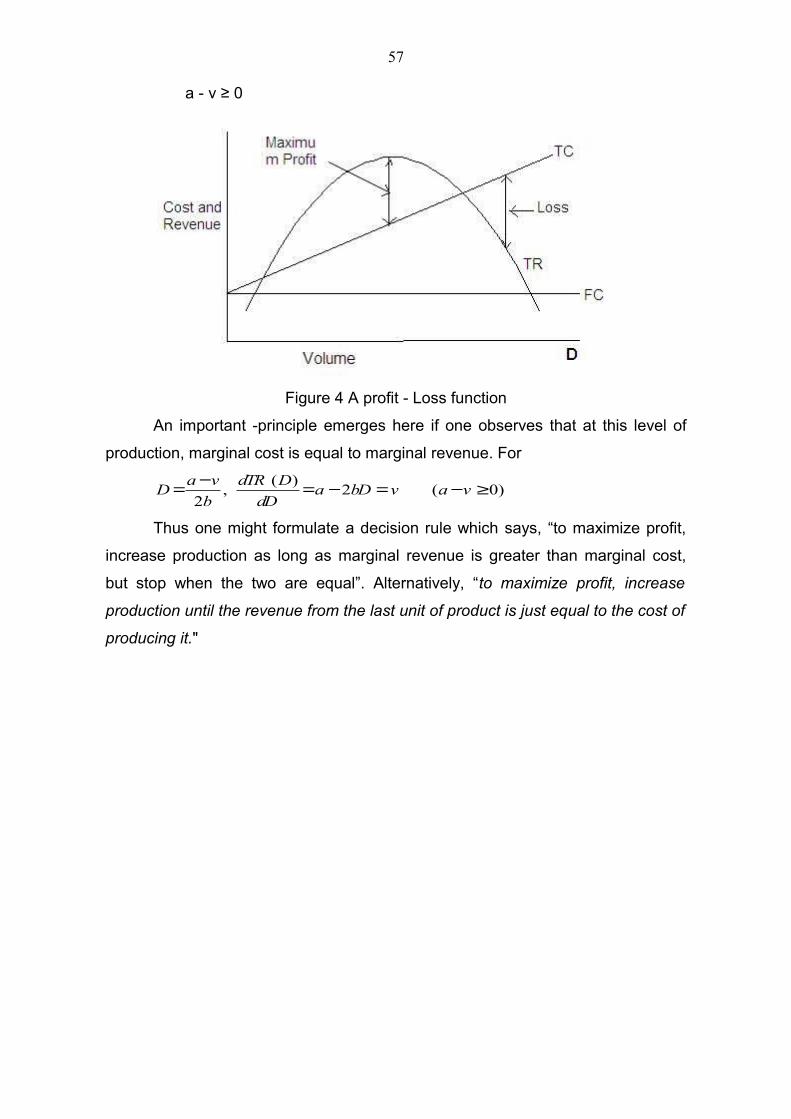
a - v ≥ 0
Figure 4 A profit - Loss function
An important -principle emerges here if one observes that at this level of
production, marginal cost is equal to marginal revenue. For
)0(2)(
,2
≥−=−=−= vavbDadD
DdTR
b
vaD
Thus one might formulate a decision rule which says, “to maximize profit,
increase production as long as marginal revenue is greater than marginal cost,
but stop when the two are equal”. Alternatively, “to maximize profit, increase
production until the revenue from the last unit of product is just equal to the cost of
producing it."
57
LECTURE NO. 15
BREAK-EVEN AND SHUTDOWN POINTS, PRODUCTION, ECONOMICS OF
MASS PRODUCTION, PRODUCTION MANAGEMENT DECISION
Break-Even and Shutdown Points
From Figure 4 certain other insights may be obtained. There are two points
at which total revenue is equal to total cost, and thus profit is zero. These points
are called the break- even points. Between the break-even points the enterprise
will make a profit, but outside of these it will suffer a loss. The lower or left-hand
break-even point is of special interest to the analysts since this is the level of,
production that must be reached to get the enterprise out of the red. Many of the
decisions of the enterprise about its activities depend heavily on the answer to the
question; "Will the venture be able to operate at or above its break-even point?"
Another decision that may confront the analyst is whether or not to cease
production entirely when conditions force volume down below the lower break-
even point. This decision might be studied using the model, although this is not
essential. Suppose the analyst finds that the enterprise is forced to produce at
some level lower than the break- even point; one then has the following
alternatives:
al = stop production
a2 = continue production at some level D1 below the break-even point
Assuming that no uncertainty or risk is involved in the analysis of this
decision, one could compute the profit associated with each alternative:
Profit
a1 — FC
a2 TR (D1) – TC (D1)
The profit for a2 may be computed as follows:
TR (D1) – TC (D1) = TR (D1) – (FC + vD1)
Alternative a2 will be preferred if
TR (D1) - (FC + vD1) > - FC
TR (D1) > vDl
Thus one has the decision rule, "so long as total revenue exceeds variable
costs, do not stop production." This rule must obviously apply in the short run,
since the enterprise cannot go on sustaining a loss for very long.
58
PRODUCTION
The problems and decisions discussed so far are largely the concern of top
management, since they are in the realm of major company policy. The analyst at
least early in the career, is more likely to be associated with decisions specifically
related to the methods of production and operation employed. Thus one may be
concerned with alternative production processes, alternative designs for the
product, alternative operating procedures, and so on.
Ideally all the decisions should be studied from the overall viewpoint of the
enterprise, with the aim of perhaps maximizing total profit as was previously
shown. For obvious practical reasons, not every decision can be approached
immediately from this viewpoint and thus one uses other, more immediate criteria.
Typically much effort is devoted to reducing costs through the improvement of the
product, the process, or the operating procedures. Although sometimes it may be
true that if costs are reduced by a rupee, profit will increase by a rupee, things are
usually not so simple. Suppose, for example, the analyst can show that by
refusing to disrupt production in order to push through "rush" orders, costs can be
reduced. Clearly profits may not be increased by an equal amount, since the
customers may take their business elsewhere. In practice many decisions are
approached from the viewpoint of minimizing costs because it may be difficult to
measure profit directly, and good judgment indicates that higher profits are likely
to result.
ECONOMIES OF MASS PRODUCTION
Suppose that management is confronted with the following decision. If the
production process and equipment are kept substantially the same, what volume
of production will minimize the average unit cost of production? This is the
question of the economic operating level for a plant. If we assume that under
these conditions the plant's costs are given by a linear total cost function, as in
Figure 1, then the average unit cost is simply given by
vD
FC
D
vDFC
D
DTCDAC +=+== )(
)(
59
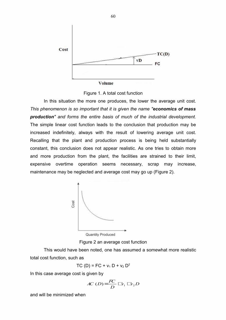
Figure 1. A total cost function
In this situation the more one produces, the lower the average unit cost.
This phenomenon is so important that it is given the name "economics of mass
production" and forms the entire basis of much of the industrial development.
The simple linear cost function leads to the conclusion that production may be
increased indefinitely, always with the result of lowering average unit cost.
Recalling that the plant and production process is being held substantially
constant, this conclusion does not appear realistic. As one tries to obtain more
and more production from the plant, the facilities are strained to their limit,
expensive overtime operation seems necessary, scrap may increase,
maintenance may be neglected and average cost may go up (Figure 2).
Figure 2 an average cost function
This would have been noted, one has assumed a somewhat more realistic
total cost function, such as
TC (D) = FC + v1 D + v2 D2
In this case average cost is given by
DvvD
FCDAC 21)( ++=
and will be minimized when
60
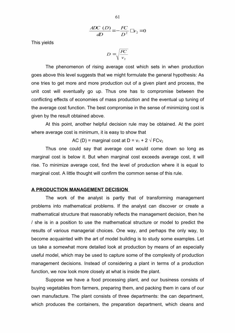
0)(
22=+−= v
D
FC
dD
DADC
This yields
2v
FCD =
The phenomenon of rising average cost which sets in when production
goes above this level suggests that we might formulate the general hypothesis: As
one tries to get more and more production out of a given plant and process, the
unit cost will eventually go up. Thus one has to compromise between the
conflicting effects of economies of mass production and the eventual up tuning of
the average cost function. The best compromise in the sense of minimizing cost is
given by the result obtained above.
At this point, another helpful decision rule may be obtained. At the point
where average cost is minimum, it is easy to show that
AC (D) = marginal cost at D = v1 + 2 √ FCv2
Thus one could say that average cost would come down so long as
marginal cost is below it. But when marginal cost exceeds average cost, it will
rise. To minimize average cost, find the level of production where it is equal to
marginal cost. A little thought will confirm the common sense of this rule.
A PRODUCTION MANAGEMENT DECISION
The work of the analyst is partly that of transforming management
problems into mathematical problems. If the analyst can discover or create a
mathematical structure that reasonably reflects the management decision, then he
/ she is in a position to use the mathematical structure or model to predict the
results of various managerial choices. One way, and perhaps the only way, to
become acquainted with the art of model building is to study some examples. Let
us take a somewhat more detailed look at production by means of an especially
useful model, which may be used to capture some of the complexity of production
management decisions. Instead of considering a plant in terms of a production
function, we now look more closely at what is inside the plant.
Suppose we have a food processing plant, and our business consists of
buying vegetables from farmers, preparing them, and packing them in cans of our
own manufacture. The plant consists of three departments: the can department,
which produces the containers, the preparation department, which cleans and
61
cooks the vegetables, and the packing department, which fills and labels the cans.
At the moment, farmers are offering both peas and tomatoes, either of which
could be processed in our plant. Our total cost and revenue structure is so simple
that we can say each can of peas yields us a profit of Rs. 5.00 and each can of
tomatoes yields a profit of Rs. 8.00. These profits are the same no matter what
level of production for either vegetable we decide on if we are planning for the
coming week, then our profit for the week will be (in Rupees).
TPoft 85Pr +=
where, P is the number of cans of peas we turn out and T is the number of cans of
tomatoes. At this point it may appear that since tomatoes are more profitable, we
should entirely forsake peas and turn out all the tomatoes possible. However,
usually things are not as simple as-that. First of all, we discover that the farmers in
the area will have available no more than the equivalent of 20,000 cans of
tomatoes and no more than the equivalent of 25,000 cans of peas. Thus our
choices of P and T are limited by the availability of vegetables. It must be that
P ≤ 25,000 T ≤ 20,000
Next, we note that the capacity of our departments is also limited. Suppose
both vegetables are packed in the same type of can, and the can department has
a capacity of 30,000 cans per week. This puts another restriction on our
production program.
P + T ≤ 30,000
The preparation department, which operates 40 hours per week, requires
0.001 hours to process enough peas to fill a can and 0.002 hours to process a
can of tomatoes. We then have a processing department restriction that says
0.001 P + 0.002 T ≤ 40
or
P + 2T ≤ 40,000
The packing department has a capacity of 50,000 cans of either type for
the week, giving
P + T ≤ 50,000
One might go on adding restrictions and conditions to make the problem
more and more realistic, but at this point the decision about a production program
is sufficiently complicated to suggest the difficulties that might be encountered.
62
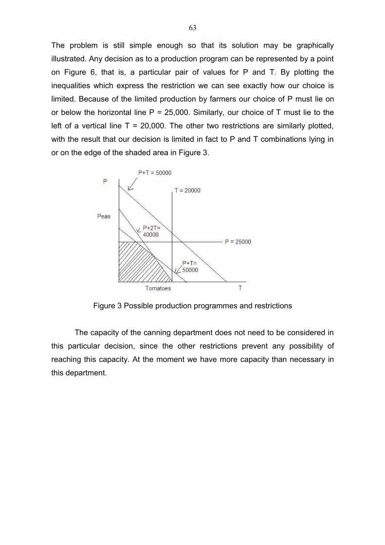
The problem is still simple enough so that its solution may be graphically
illustrated. Any decision as to a production program can be represented by a point
on Figure 6, that is, a particular pair of values for P and T. By plotting the
inequalities which express the restriction we can see exactly how our choice is
limited. Because of the limited production by farmers our choice of P must lie on
or below the horizontal line P = 25,000. Similarly, our choice of T must lie to the
left of a vertical line T = 20,000. The other two restrictions are similarly plotted,
with the result that our decision is limited in fact to P and T combinations lying in
or on the edge of the shaded area in Figure 3.
Figure 3 Possible production programmes and restrictions
The capacity of the canning department does not need to be considered in
this particular decision, since the other restrictions prevent any possibility of
reaching this capacity. At the moment we have more capacity than necessary in
this department.
63
LECTURE NO. 16
PLANT LAYOUT: IMPORTANCE, FLOW PATTERNS
Importance and Function
Plant layout refers to an optimum arrangement of different facilities
including human resource, plant and machinery, material etc. Since a layout
once implemented cannot be easily changed and costs of such a change are
substantial, the plant layout is a strategic decision. A poor layout will result in
continuous losses in terms of higher efforts for material handling, more waste and
rework, poor space utilization etc. Hence, need to analyze and design a sound
plant layout can hardly be over emphasized. It is a crucial function that has to be
performed both at the time of initial design of any facility, and during its growth,
development and diversification.
The problem of plant layout should be seen in relation to overall plant design
which includes many other functions such as product design, sales planning,
selection of the production process, plant size, plant location, building,
diversification etc. The layout problem occurs because of many developments
including:
• change in product design
• introduction of new product
• obsolescence of facilities
• changes in demand
• market changes
• competitive cost reduction
• frequent accidents
• adoption of new safety standards
• decision to build a new plant
Plant layout problem is defined by Moore (1962) as follows: “plant layout is a
plan of, or the act of planning, an optimum arrangement of facilities, including
personnel, operating equipment storage space, materials handling equipment,
and all other supporting services, along with the design of the best structure to
contain these facilities”.
64
Objectives and advantages
Some of the important objectives of a good plant layout are as follows:
• Overall simplification of production process in terms of equipment
utilization, minimization of delays, reducing manufacturing time, and better
provisions for maintenance
• Overall integration of man, materials, machinery, supporting activities
and any other considerations in a way that result in the best
compromise.
• Minimization of material handling cost by suitably placing the facilities in
the best flow sequence
• Saving in floor space, effective space utilization and less congestion /
confusion,
• Increased output and reduced in-process inventories
• Better supervision and control
• Worker convenience and worker satisfaction
• Better working environment, safety of employees and reduced hazards
• minimization of waste and higher productivity
• avoid unnecessary capital investment
• higher flexibility and adaptability to changing conditions
Types of layout Problems
The plant layout problems can be classified into four types as follows:
• Planning completely new facility
• Expanding or relocating an existing facility
• Rearrangement of existing layout
• Minor modifications in present layout
Flow Patterns
According to the principle of flow, the layout plan arranges the work area
for each operation or process so as to have an overall smooth flow through the
production / service facility. The basic types of flow patterns that are employed in
designing the layout are I-flow, L-flow, U- flow, S-flow and O - flow as shown in
Figure 1. These are briefly explained below:
65
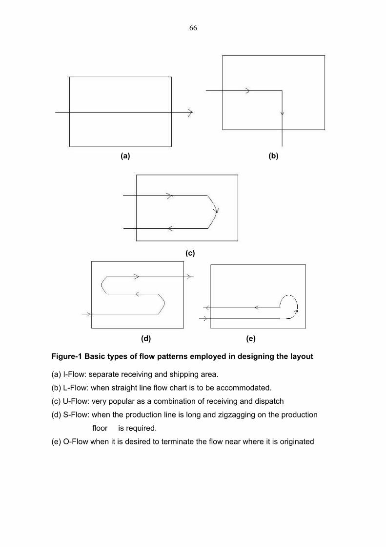
(a) (b)
(c)
(d) (e)
Figure-1 Basic types of flow patterns employed in designing the layout
(a) I-Flow: separate receiving and shipping area.
(b) L-Flow: when straight line flow chart is to be accommodated.
(c) U-Flow: very popular as a combination of receiving and dispatch
(d) S-Flow: when the production line is long and zigzagging on the production
floor is required.
(e) O-Flow when it is desired to terminate the flow near where it is originated
66
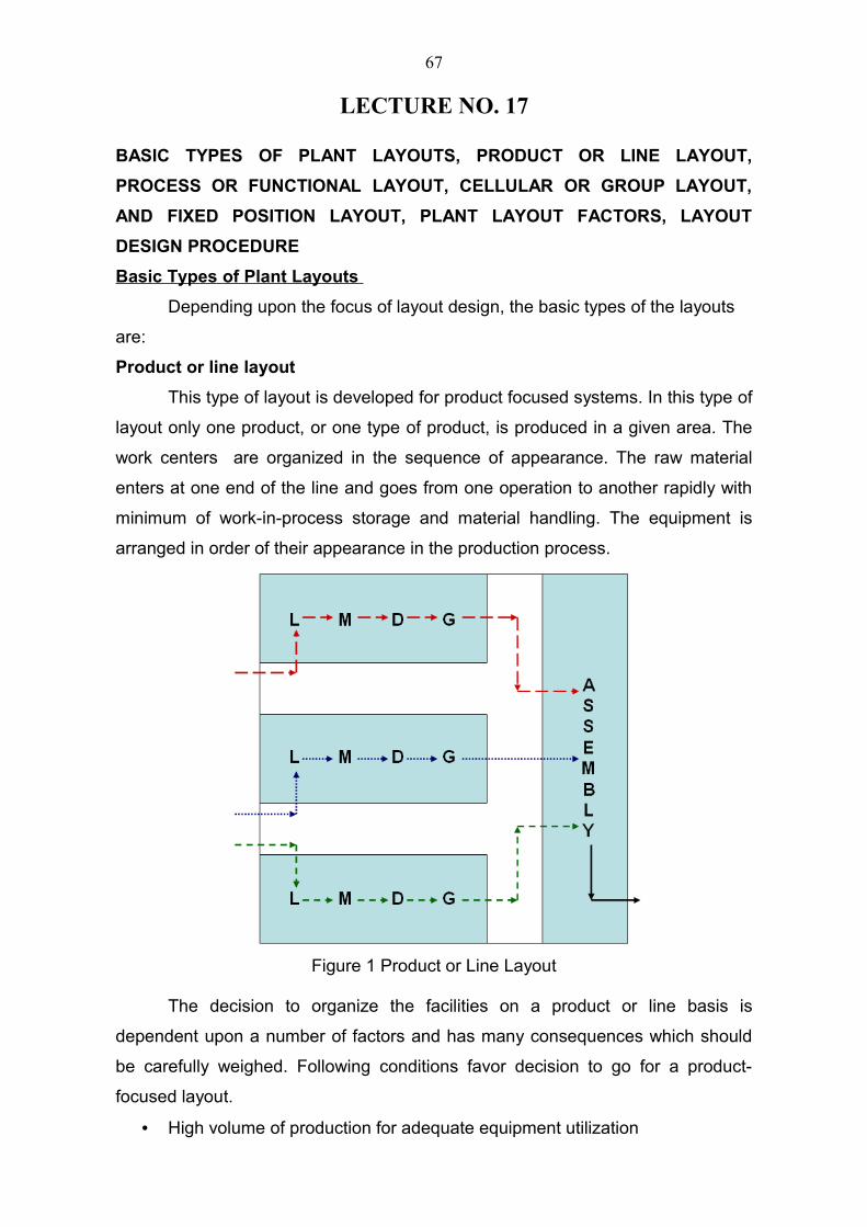
LECTURE NO. 17
BASIC TYPES OF PLANT LAYOUTS, PRODUCT OR LINE LAYOUT,
PROCESS OR FUNCTIONAL LAYOUT, CELLULAR OR GROUP LAYOUT,
AND FIXED POSITION LAYOUT, PLANT LAYOUT FACTORS, LAYOUT
DESIGN PROCEDURE
Basic Types of Plant Layouts
Depending upon the focus of layout design, the basic types of the layouts
are:
Product or line layout
This type of layout is developed for product focused systems. In this type of
layout only one product, or one type of product, is produced in a given area. The
work centers are organized in the sequence of appearance. The raw material
enters at one end of the line and goes from one operation to another rapidly with
minimum of work-in-process storage and material handling. The equipment is
arranged in order of their appearance in the production process.
Figure 1 Product or Line Layout
The decision to organize the facilities on a product or line basis is
dependent upon a number of factors and has many consequences which should
be carefully weighed. Following conditions favor decision to go for a product-
focused layout.
• High volume of production for adequate equipment utilization
67
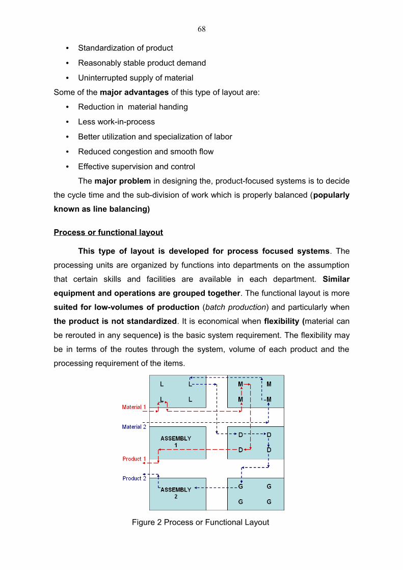
• Standardization of product
• Reasonably stable product demand
• Uninterrupted supply of material
Some of the major advantages of this type of layout are:
• Reduction in material handing
• Less work-in-process
• Better utilization and specialization of labor
• Reduced congestion and smooth flow
• Effective supervision and control
The major problem in designing the, product-focused systems is to decide
the cycle time and the sub-division of work which is properly balanced (popularly
known as line balancing)
Process or functional layout
This type of layout is developed for process focused systems. The
processing units are organized by functions into departments on the assumption
that certain skills and facilities are available in each department. Similar
equipment and operations are grouped together. The functional layout is more
suited for low-volumes of production (batch production) and particularly when
the product is not standardized. It is economical when flexibility (material can
be rerouted in any sequence) is the basic system requirement. The flexibility may
be in terms of the routes through the system, volume of each product and the
processing requirement of the items.
Figure 2 Process or Functional Layout
68
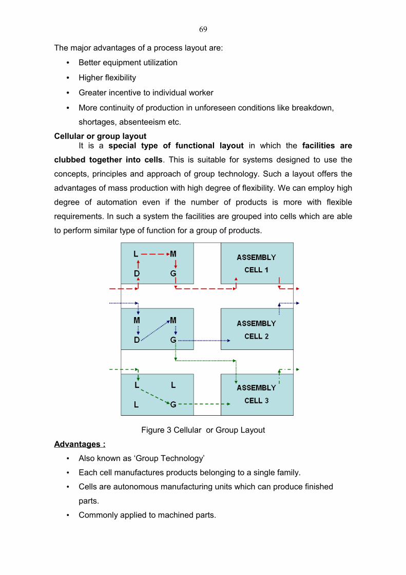
The major advantages of a process layout are:
• Better equipment utilization
• Higher flexibility
• Greater incentive to individual worker
• More continuity of production in unforeseen conditions like breakdown,
shortages, absenteeism etc.
Cellular or group layoutIt is a special type of functional layout in which the facilities are
clubbed together into cells. This is suitable for systems designed to use the
concepts, principles and approach of group technology. Such a layout offers the
advantages of mass production with high degree of flexibility. We can employ high
degree of automation even if the number of products is more with flexible
requirements. In such a system the facilities are grouped into cells which are able
to perform similar type of function for a group of products.
Figure 3 Cellular or Group Layout
Advantages :
• Also known as ‘Group Technology’
• Each cell manufactures products belonging to a single family.
• Cells are autonomous manufacturing units which can produce finished
parts.
• Commonly applied to machined parts.
69
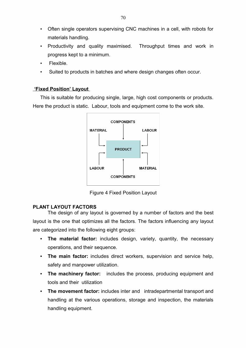
• Often single operators supervising CNC machines in a cell, with robots for
materials handling.
• Productivity and quality maximised. Throughput times and work in
progress kept to a minimum.
• Flexible.
• Suited to products in batches and where design changes often occur.
‘Fixed Position’ Layout
This is suitable for producing single, large, high cost components or products.
Here the product is static. Labour, tools and equipment come to the work site.
Figure 4 Fixed Position Layout
PLANT LAYOUT FACTORS The design of any layout is governed by a number of factors and the best
layout is the one that optimizes all the factors. The factors influencing any layout
are categorized into the following eight groups:
• The material factor: includes design, variety, quantity, the necessary
operations, and their sequence.
• The main factor: includes direct workers, supervision and service help,
safety and manpower utilization.
• The machinery factor: includes the process, producing equipment and
tools and their utilization
• The movement factor: includes inter and intradepartmental transport and
handling at the various operations, storage and inspection, the materials
handling equipment.
70
• The waiting factor: includes permanent and temporary storage and delays
and their locations.
• The service factors: include service relating to employee facilities such as
parking lot, locker rooms, toilets, waiting rooms etc.; service relating to
materials in terms of quality, production control, scheduling, dispatching,
waste control; and service relating to machinery such as maintenance.
• The building factor: includes outside and inside building features and
utility distribution and equipment.
• The change factor: includes versatility, flexibility and expansion
Each of the above mentioned factors comprise a number of features and
the layout engineer must review these in the light of his problem. Usually the
layout design process is a compromise of these various considerations to meet
the overall objectives in the best possible manner.
LAYOUT DESIGN PROCEDURE
The overall layout design procedure can be considered to be composed of
four phases Viz.,
Phase I: Location
Phase II: General Overall Layout
Phase III: Detailed layout
Phase IV: Installation
Some important guidelines that help in the layout design are:
• Plan from whole to details
• First plan the ideal and then move to the practical aspects
• Material requirements should be central to the planning of process and
machinery .
• modify the process and machinery by different factors to plan the layout
Though there is always an overlap in the different phases of layout design the
major steps that have to be followed in the layout design are outlined as
follows:
• state the problem in terms of its objective, scope and factors to be
considered
71
• Collect basic data on sales forecasts, production volumes, production
schedules, part lists, operations to be performed, work measurement,
existing layouts, building drawing etc.
• Analyze data and present it in the form of various charts
• Plan the production process and its arrangement
• Plan the material flow pattern and develop the overall material-handling
plan
• Estimate plant and machinery requirements
• Select material handling equipment
• Determine storage requirements
• Design and plan activity relationships
• Plan auxiliary and service facilities including their arrangement
• Determine space requirements and allocate activity areas
• Develop plot plan and block plan i.e. integrate all plant operations
• Develop detailed layouts and plan building along with its arrangement
• Evaluate, modify and check the layouts
• Install layouts and follow up
The Systematic Layout Planning (SLP) procedure as presented by Francis
and White (1974) is shown in Figure-5. We see that once the appropriate
information is gathered, a flow analysis can be combined with an activity analysis
to develop the relationship diagram. Space considerations when combined with
the relationship diagram lead to the construction of the space relationship
diagram. Based on the space relationship diagram modifying considerations and
practical limitations, a number of alternative layouts are designed and evaluated.
Data collection The development of any layout is dependent on the quality and quantity of
facts that we have about the various factors influencing it. The data collection
phase is not a one-time effort but an ongoing function. The data for overall plan is
to be collected at initial stages where as the data for detailed layouts may be
obtained at a later stage, the facts have to be obtained regarding various
materials and processes, the flow routing and sequencing, space requirements
and different activities and relationships.
72
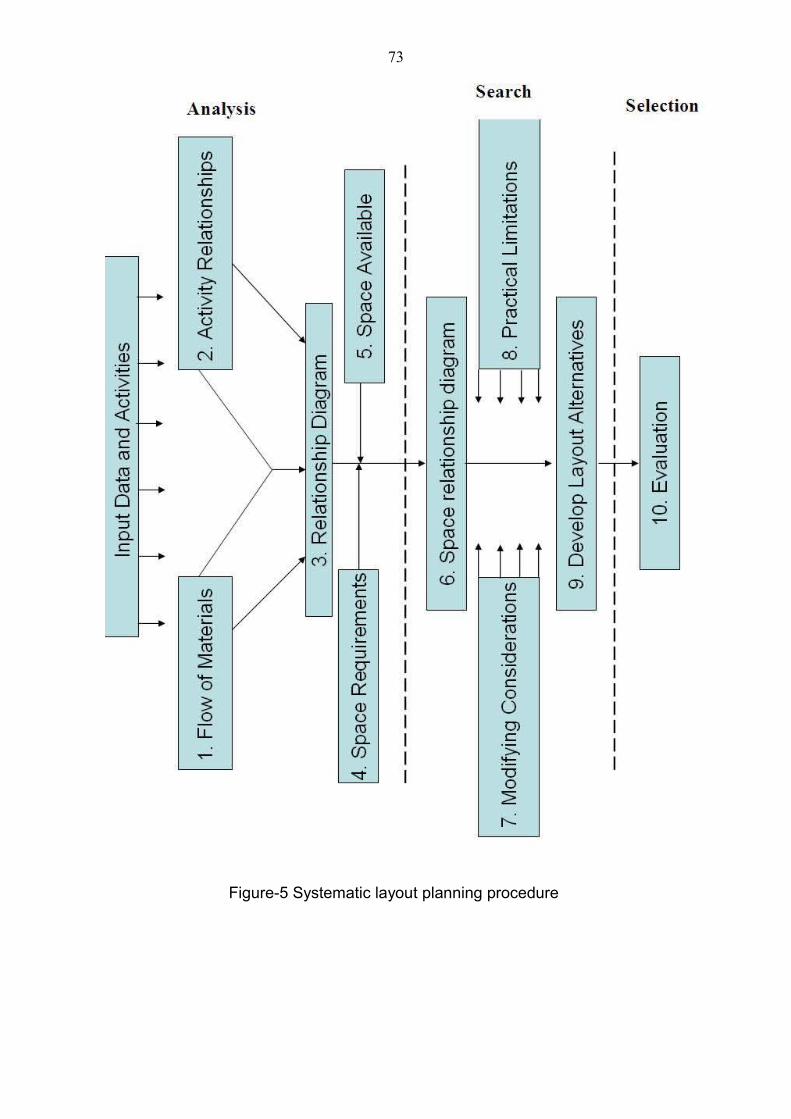
Figure-5 Systematic layout planning procedure
73
LECTURE NO. 18
GENERAL GUIDE LINES FOR PLANT LAYOUT, TYPICAL CLEARANCES,
AREAS AND ALLOWANCES, PLANT LAYOUT, LAYOUT OF EQUIPMENT,
SPACE DETERMINATION
General Guidelines / considerations
Site layout: A good site layout provides safe and economical flow of materials and
personnel. A material sheet for the site is therefore prepared which then allows
the various processes to be positioned relative to one another. The services (e.g.
boiler house, effluent plant etc.) are then added in the most convenient positions.
The central buildings (administration, canteen, laboratories etc.) are placed in
such a manner that the distances traveled by personnel to use them are
minimized. Finally the road and rail systems are marked in. Typical sizes and
clearances for the site layout are given in Tables 1 to 3. Having established site
constraints and standards, a more detailed site layout can be made. The site
layout thus prepared should then be considered to see whether the layout is
consistent with safety requirements and that it assists action in any emergency as
also the constraints and standards have not been violated.
Broad guidelines for preparation of the site layout are given below:
• Minimize the distance that materials have to travel to or from stores or
during processing
• Separate the raw material unloading and finished product loading
facilities
• Isolate the hazardous operations
• Locate storage areas close to unloading and loading facilities
• locate boiler room, power station, cooling towers, water pumping station
etc. on periphery but adjacent to the area of largest use
• The usual clearances between pipes including flanges and lagging and
between pipes and other objects should be 25 mm but this should be
increased if hot pipes run near plastic pipes, cables etc.
• Steam and water mains, electricity and telephone cables etc. should, in
general, run parallel to the road system and should avoid going through
plant area
74
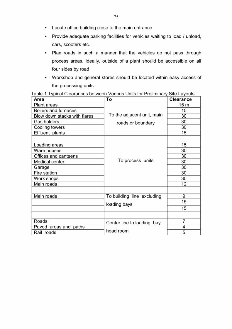
• Locate office building close to the main entrance
• Provide adequate parking facilities for vehicles waiting to load / unload,
cars, scooters etc.
• Plan roads in such a manner that the vehicles do not pass through
process areas. Ideally, outside of a plant should be accessible on all
four sides by road
• Workshop and general stores should be located within easy access of
the processing units.
Table-1 Typical Clearances between Various Units for Preliminary Site Layouts Area To ClearancePlant areas
To the adjacent unit, main
roads or boundary
15 mBoilers and furnaces 15Blow down stacks with flares 30Gas holders 30Cooling towers 30Effluent plants 15
Loading areas
To process units
15Ware houses 30Offices and canteens 30Medical center 30Garage 30Fire station 30Work shops 30Main roads 12
Main roads To building line excluding
loading bays
91515
Roads Center line to loading bay
head room
7Paved areas and paths 4Rail roads 5
75
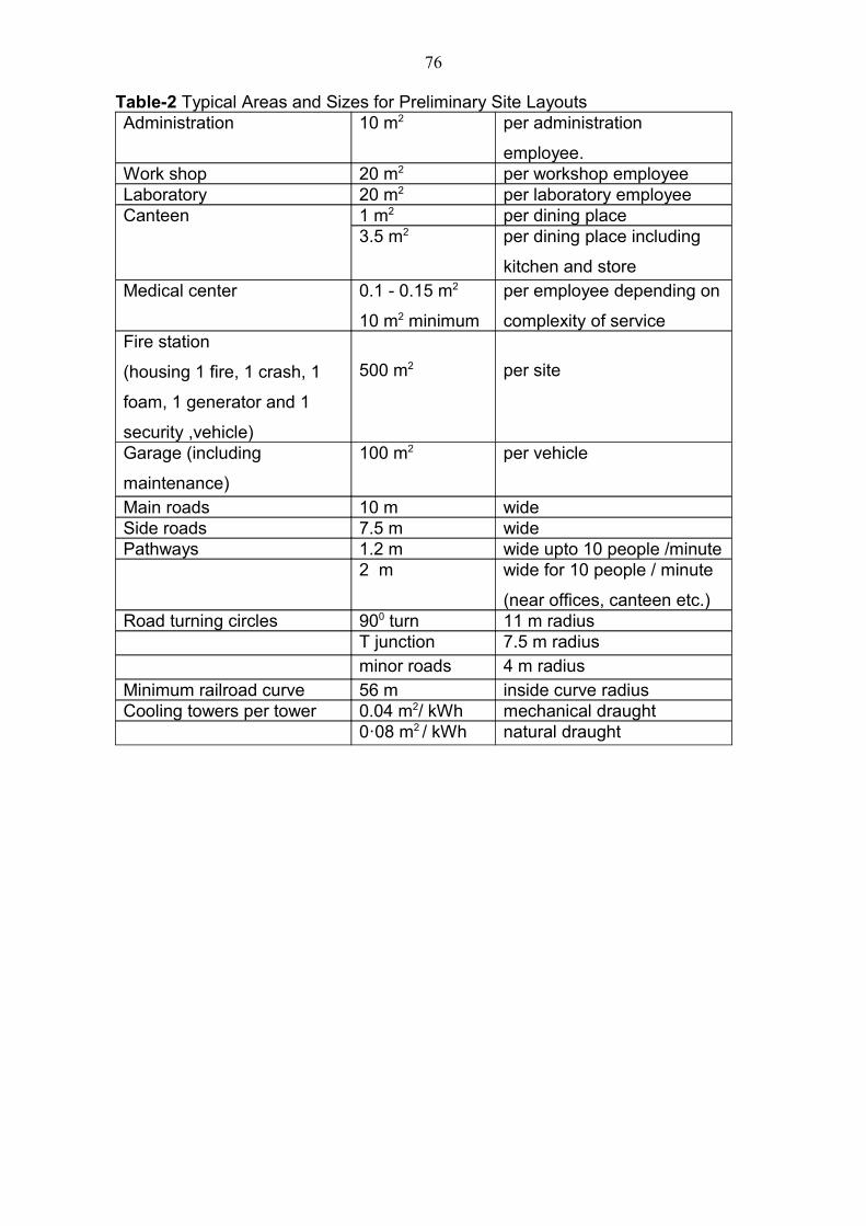
Table-2 Typical Areas and Sizes for Preliminary Site Layouts Administration 10 m2 per administration
employee. Work shop 20 m2 per workshop employee Laboratory 20 m2 per laboratory employee Canteen 1 m2 per dining place
3.5 m2 per dining place including
kitchen and store Medical center 0.1 - 0.15 m2
10 m2 minimum
per employee depending on
complexity of service Fire station
(housing 1 fire, 1 crash, 1
foam, 1 generator and 1
security ,vehicle)
500 m2 per site
Garage (including
maintenance)
100 m2 per vehicle
Main roads 10 m wideSide roads 7.5 m widePathways 1.2 m wide upto 10 people /minute
2 m wide for 10 people / minute
(near offices, canteen etc.) Road turning circles 900 turn 11 m radius
T junction 7.5 m radius minor roads 4 m radius
Minimum railroad curve 56 m inside curve radius Cooling towers per tower 0.04 m2/ kWh mechanical draught
0·08 m2 / kWh natural draught
76
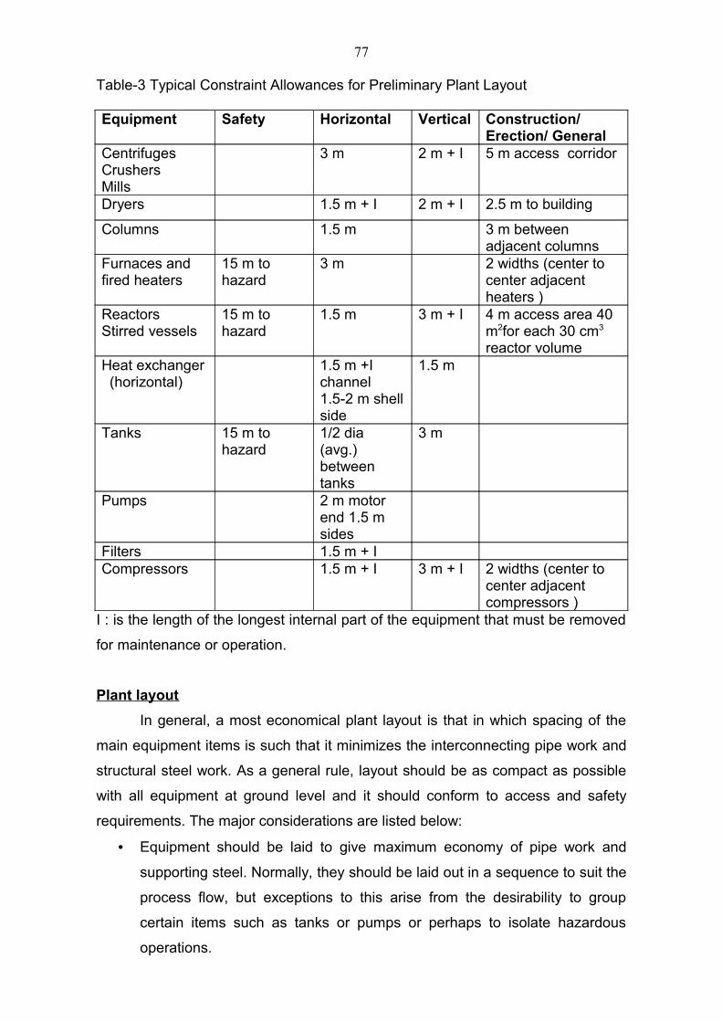
Table-3 Typical Constraint Allowances for Preliminary Plant Layout
Equipment Safety Horizontal Vertical Construction/Erection/ General
Centrifuges CrushersMills
3 m 2 m + I 5 m access corridor
Dryers 1.5 m + I 2 m + I 2.5 m to building
Columns 1.5 m 3 m between adjacent columns
Furnaces and fired heaters
15 m to hazard
3 m 2 widths (center to center adjacent heaters )
ReactorsStirred vessels
15 m to hazard
1.5 m 3 m + I 4 m access area 40 m2for each 30 cm3
reactor volumeHeat exchanger (horizontal)
1.5 m +I channel1.5-2 m shell side
1.5 m
Tanks 15 m to hazard
1/2 dia(avg.) between tanks
3 m
Pumps 2 m motor end 1.5 m sides
Filters 1.5 m + ICompressors 1.5 m + I 3 m + I 2 widths (center to
center adjacent compressors )
I : is the length of the longest internal part of the equipment that must be removed
for maintenance or operation.
Plant layout
In general, a most economical plant layout is that in which spacing of the
main equipment items is such that it minimizes the interconnecting pipe work and
structural steel work. As a general rule, layout should be as compact as possible
with all equipment at ground level and it should conform to access and safety
requirements. The major considerations are listed below:
• Equipment should be laid to give maximum economy of pipe work and
supporting steel. Normally, they should be laid out in a sequence to suit the
process flow, but exceptions to this arise from the desirability to group
certain items such as tanks or pumps or perhaps to isolate hazardous
operations.
77
• In general, high elevation should only be considered when ground space is
limited or where gravity flow of materials is desired.
• Equipment items which are considered to be a source of hazard should be
grouped together and wherever possible should be located separately from
other areas of the plant.
• Provide sufficient clear space between critical and mechanically dangerous
or high temperature equipment to allow safety of operating or maintenance
personnel.
• The equipment needing frequent internal cleaning or replacement of
internal parts should be laid out for ease of maintenance.
• Elevation to the underside of the pipe bridges and racks over paved areas
should be at least 4 m.
Layout of equipment
Thought should be given to the location of equipment requiring frequent
attendance by operating personnel and the relative position the control room to
obtain the shortest and most direct routes for operators when on route operation.
However, the control room should be in a safe area. Some important
considerations involved in locating a few key equipment items are listed below:
• Mixing vessels can be laid out in a straight line, in pairs or staggered.
• In evaporators using barometric leg type condensers, barometric leg
should be at least 10 mm from the vessel base. This is usually situated on
the ground floor. For multiple effect evaporators, place the individual effects
as close as possible to minimize vapor lines. Vapor liquid separator is
accommodated without increasing the distance between effects. The layout
requirements for crystallizers are similar to those for evaporators.
• Furnaces should be located at least 15 m away from other equipment.
Ample room need to be provided at the firing front for the operation of the
burner and burner control panel.
• Where there are a large number of heat exchangers, they are often put
together in one or more groups. Location should provide a layout, which is
convenient to operate and maintain. Horizontal clearance of at least 1.5 m
should be left between exchangers or exchangers and piping. Floating
head heat exchangers require an installation length of at least 2.5 times the
78
tube length. Air cooled exchangers are located adjacent to the plant section
they serve.
• Pumps in general should be located close to the equipment from which
they take suction. Changes in direction of the suction line should be at least
0.6 m from the pump. As far as possible, clearances and piping should
provide free access to one side of the motor and pump. Clearances
between pumps or pumps and piping should be at least 1.2 m for small
pumps (18 kW) and 1.5 m to 2 m for large pumps. Pumps handling hot
liquid (60 °C) should be at least 7.5 m from pumps handling volatile liquids.
Space Determination In the layout planning process the space is allotted to different activities.
The theoretical minimum space, a plant can occupy, is the total volume of its
various components. Various constraints prevent the attainment of this minimum.
Such constraints include allowing adequate clearances for access during
operation and maintenance and to allow safe operation. While determining the
space consideration should be given to the following.
• Operating equipment • Storage • Service facilities • Operators/workers
Allowance must be made for space between adjacent equipment/machines
for movement of the worker, work-in-process, maintenance personnel etc.
79
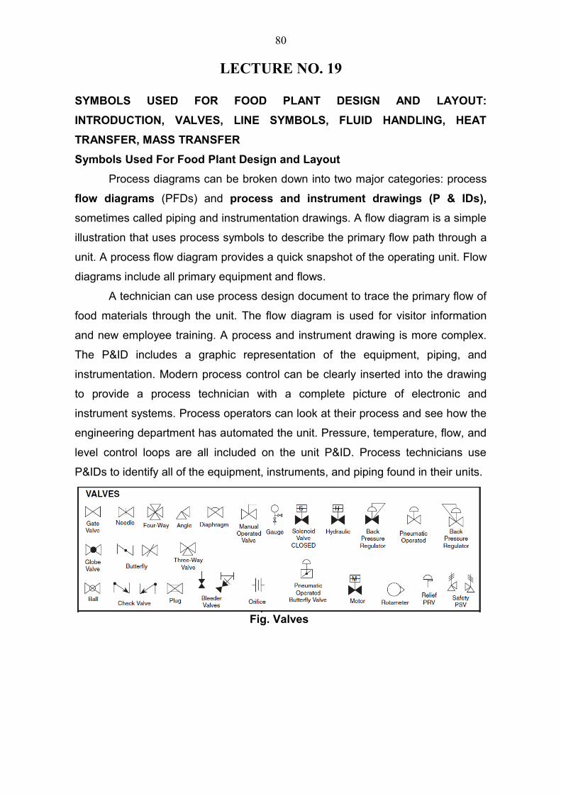
LECTURE NO. 19
SYMBOLS USED FOR FOOD PLANT DESIGN AND LAYOUT:
INTRODUCTION, VALVES, LINE SYMBOLS, FLUID HANDLING, HEAT
TRANSFER, MASS TRANSFER
Symbols Used For Food Plant Design and Layout
Process diagrams can be broken down into two major categories: process
flow diagrams (PFDs) and process and instrument drawings (P & IDs),
sometimes called piping and instrumentation drawings. A flow diagram is a simple
illustration that uses process symbols to describe the primary flow path through a
unit. A process flow diagram provides a quick snapshot of the operating unit. Flow
diagrams include all primary equipment and flows.
A technician can use process design document to trace the primary flow of
food materials through the unit. The flow diagram is used for visitor information
and new employee training. A process and instrument drawing is more complex.
The P&ID includes a graphic representation of the equipment, piping, and
instrumentation. Modern process control can be clearly inserted into the drawing
to provide a process technician with a complete picture of electronic and
instrument systems. Process operators can look at their process and see how the
engineering department has automated the unit. Pressure, temperature, flow, and
level control loops are all included on the unit P&ID. Process technicians use
P&IDs to identify all of the equipment, instruments, and piping found in their units.
Fig. Valves
80
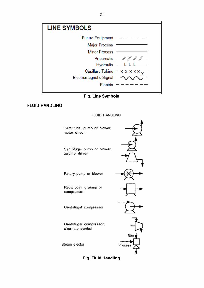
Fig. Line Symbols
FLUID HANDLING
Fig. Fluid Handling
81
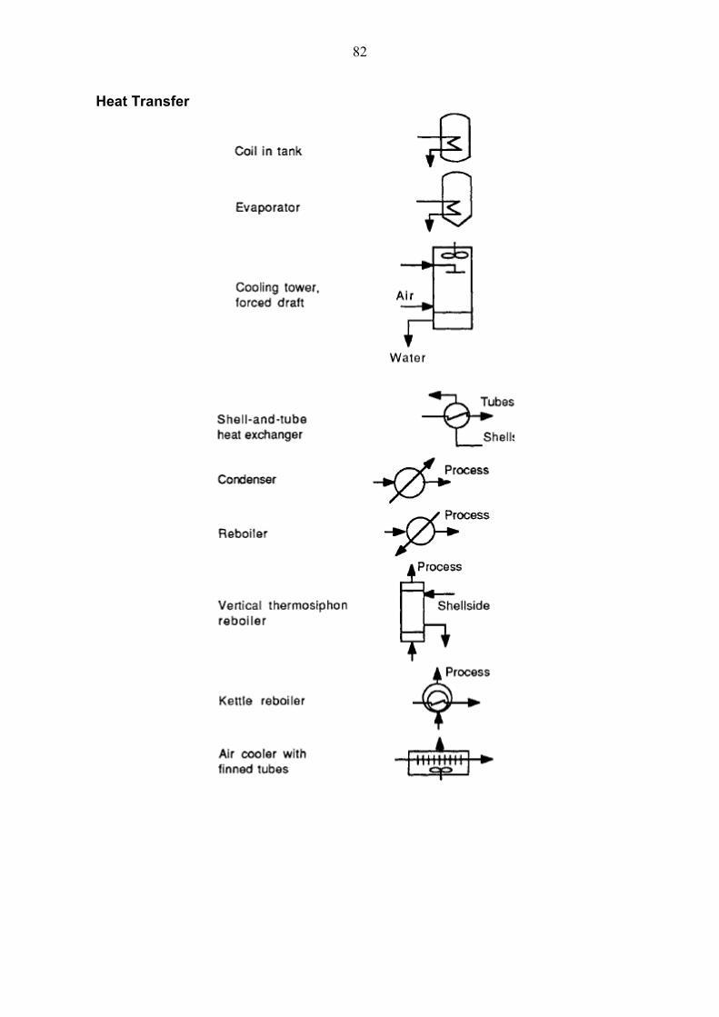
Heat Transfer
82
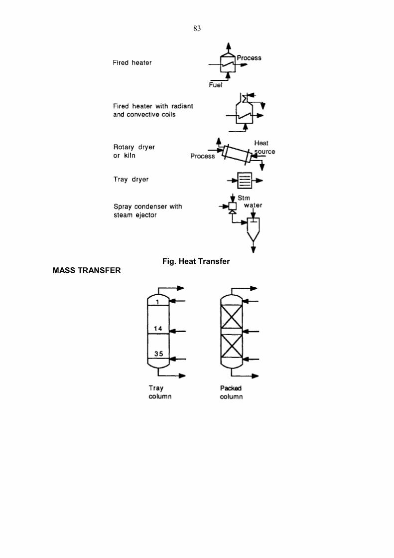
Fig. Heat TransferMASS TRANSFER
83
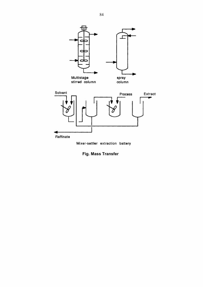
Fig. Mass Transfer
84
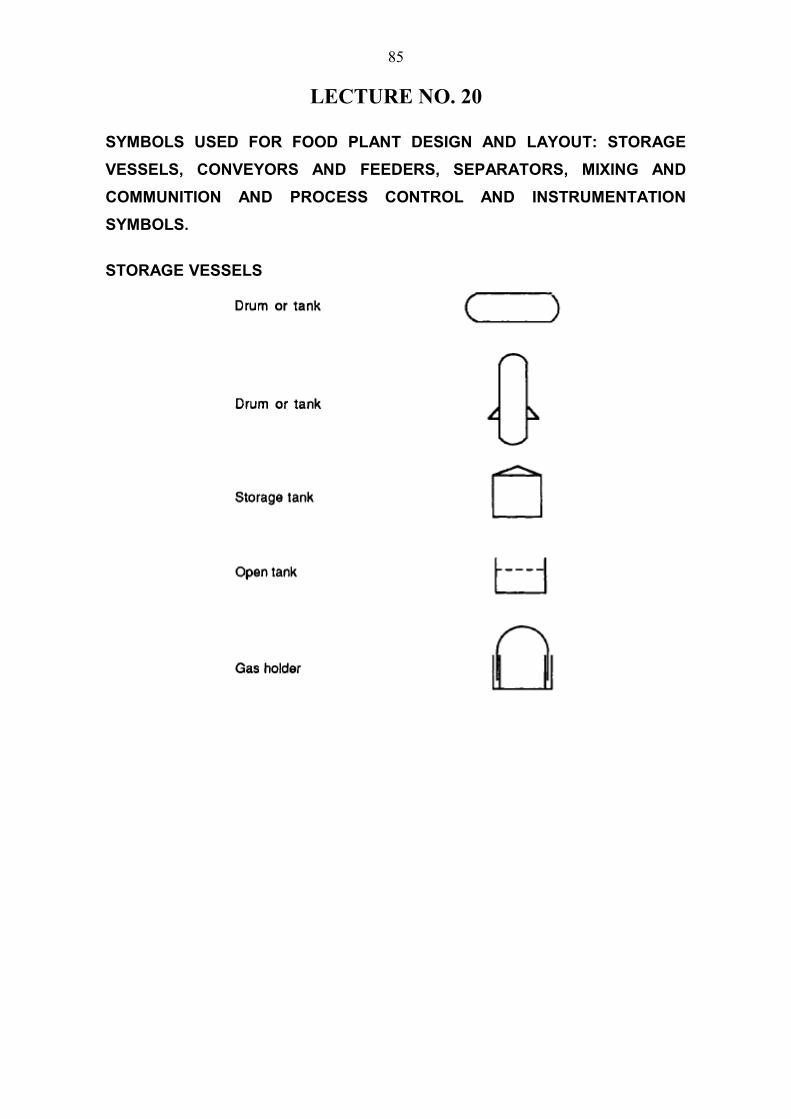
LECTURE NO. 20
SYMBOLS USED FOR FOOD PLANT DESIGN AND LAYOUT: STORAGE
VESSELS, CONVEYORS AND FEEDERS, SEPARATORS, MIXING AND
COMMUNITION AND PROCESS CONTROL AND INSTRUMENTATION
SYMBOLS.
STORAGE VESSELS
85
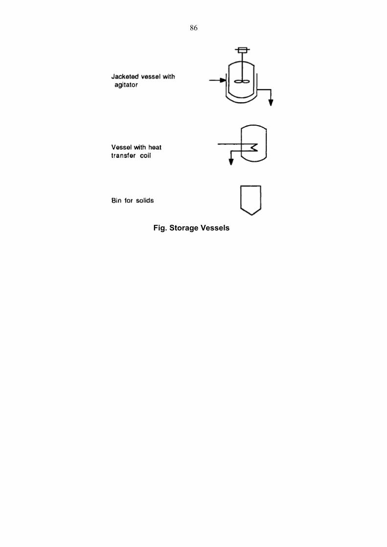
Fig. Storage Vessels
86
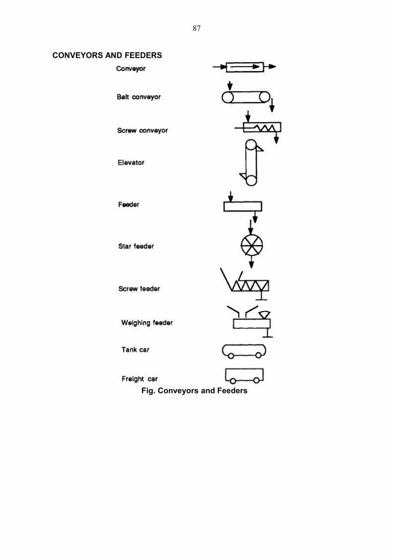
CONVEYORS AND FEEDERS
Fig. Conveyors and Feeders
87
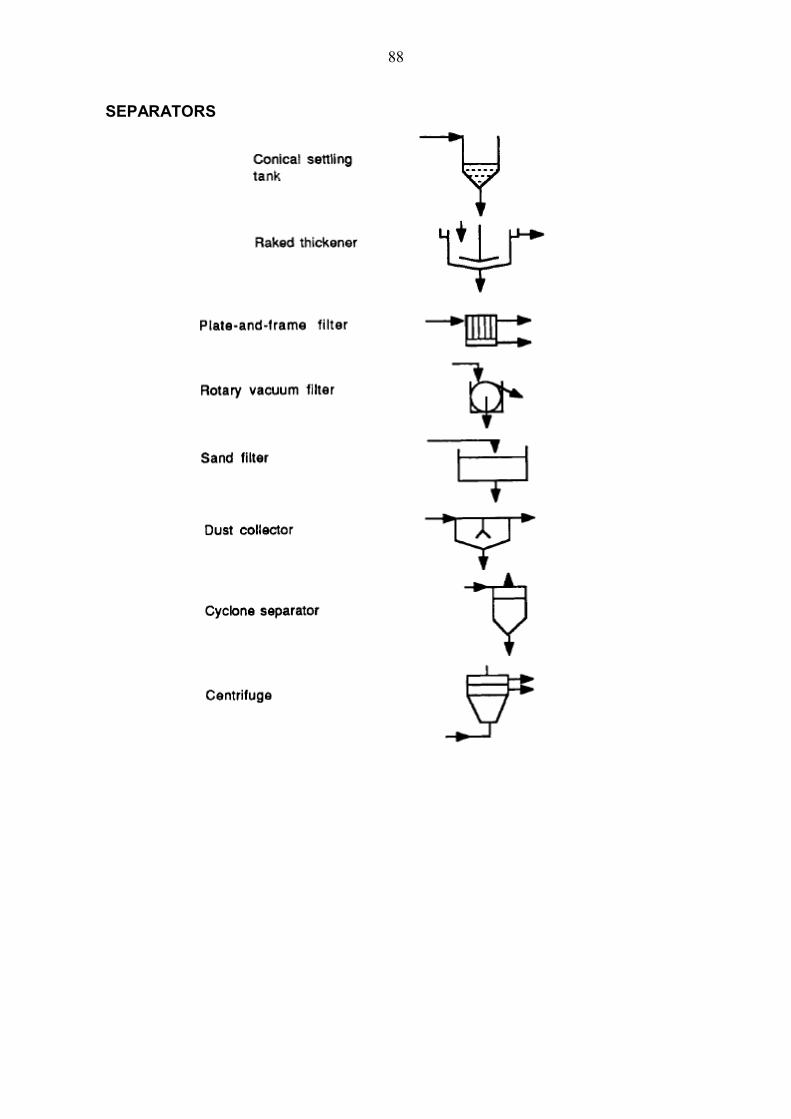
SEPARATORS
88
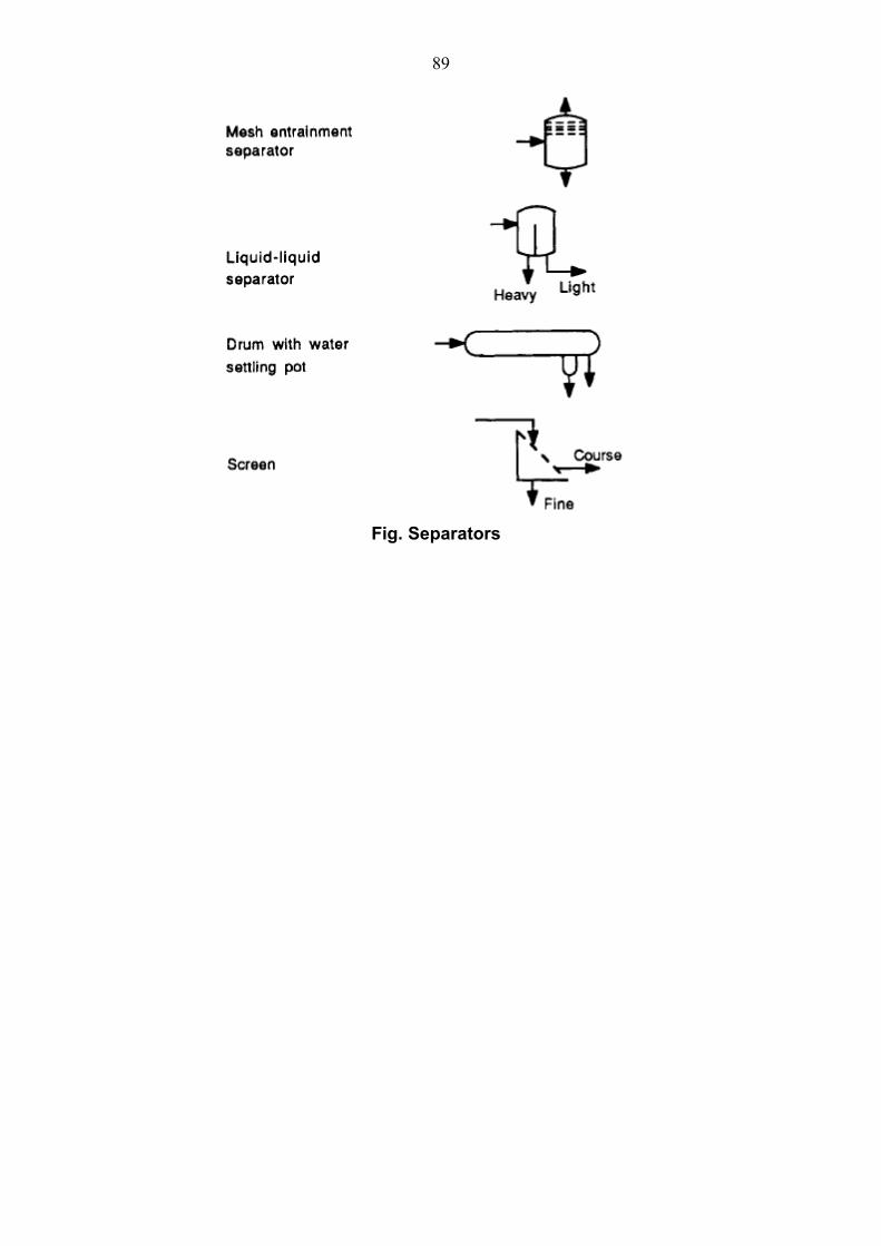
Fig. Separators
89
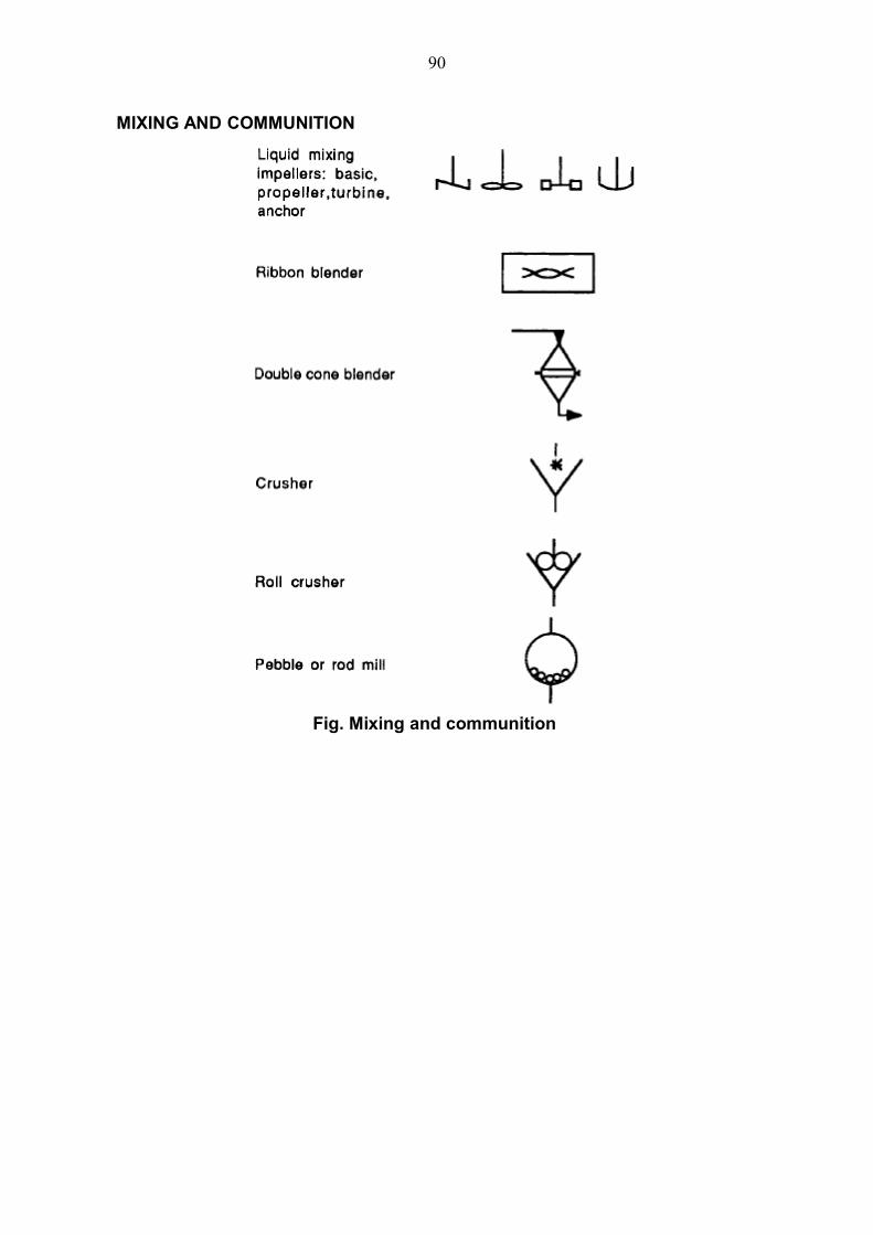
MIXING AND COMMUNITION
Fig. Mixing and communition
90
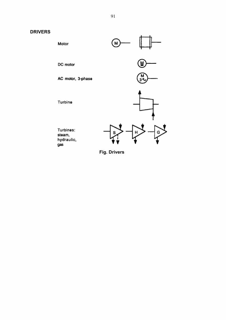
DRIVERS
Fig. Drivers
91
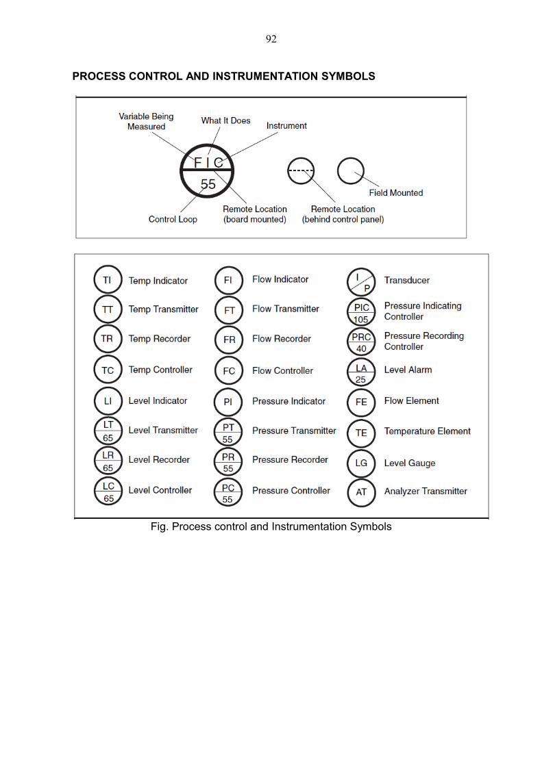
PROCESS CONTROL AND INSTRUMENTATION SYMBOLS
Fig. Process control and Instrumentation Symbols
92
LECTURE NO. 21
EXPERIMENTATION IN PILOT LAYOUT: SIZE AND STRUCTURE OF THE
PILOT PLANT, MINIMUM AND MAXIMUM SIZE, TYPES AND APPLICATIONS
Experimentation in Pilot Plant
The pilot plant is a physical model and should be a “copy” of the
corresponding industrial unit, with equipment scaled down in size to approximately
1/100 – 1/10 of the modeled unit.
Pilot plant experiments serve to obtain more information and data in the
following areas:
1. Market survey: A determined new product amount can be produced in the pilot
plant, to test its acceptance and to decide whether it would be economically
profitable.
2. Design data: The behavior of a given operation or unit process can be found
under conditions impossible to duplicate in the laboratory.
3. Products and raw materials: A pilot plant is usually needed to characterize
food products and to evaluate the development of certain raw materials into
specific products.
4. Optimization data of a running plant.
SIZE AND STRUCTURE OF THE PILOT PLANT
Basic Principles of Scaling
The most important criterion in determining the size and form of a pilot
plant is the principle of similarity, a principle first formulated by Newton.
If, fluids are handled in the pilot plant, three types of similarities involved in
fluid dynamics must be included:
1. Geometric similarity. Both the pilot plant and food processing plant
should have the same physical form or at least the same geometric
dimension relationships.
2. Kinematic similarity. The same velocity relationships should exist in both
the pilot and food processing plants.
3. Dynamic similarity: In both the pilot and food processing plants, the same
force relationships should exist. For example, the turbulence regime should be
similar on both scales when fluids are handled.
93
If the process simulated in a pilot plant involves chemical the following
similarities apply:
1. Thermal similarity.
2. Chemical and biochemical similarity.
Minimum and Maximum SizeSeveral factors can affect the size of a pilot plant. In general, the minimum
size is set by the minimum product amount required for quality analytical control.
The maximum size of the pilot plant is set by the amount of processed
product needed in order to test market acceptance.
Types and ApplicationsWhen product production in amounts large enough to conduct market
acceptance tests is required, the pilot plant is called a semi-commercial plant.
Applications
The most common applications of a pilot plant are as follows:
1. Product studies
• Quality characterization
• Influence of process conditions on product quality
• Development of new products
• Studies of market acceptance
2. Raw material studies
• Raw material characterization
• Evaluation of aptitude for industrialization of different raw materials
3. Process technology and engineering studies
• Setting the most suitable process conditions from an economic
point of view (cost minimization) and a product quality point of view
(to obtain a product of given quality). Process technology is
optimized.
• Study of process equipment alternatives to carry out given food
processing steps or unit operations.
• Development of new process technology.
• Development of new process engineering or process equipment.
4. Auxiliary system requirement studies
• Reliable evaluation of mass and energy balances and food
physical properties
• Study of energy recovery possibilities in process systems
• Improvement and evaluation of alternatives for control systems
94
LECTURE NO. 22
ENGINEERING ECONOMY : INTRODUCTION, TERMS: TIME VALUE OF
MONEY, INFLATION, INTEREST, INTEREST RATE, COMPOUND INTEREST,
RATE OF RETURN, PAYMENT, RECEIPT , CASH FLOW, PRESENT VALUE,
EQUIVALENCE, SUNK COSTS, OPPORTUNITY COSTS, ASSET, LIFE OF AN
ASSET, DEPRECIATION, BOOK VALUE OF AN ASSET, SALVAGE VALUE,
RETIREMENT, REPLACEMENT, DEFENDER AND CHALLENGER.
Introduction
Engineering Economy is the study of quantitative techniques
for the evaluation of engineering alternatives based upon financial criteria.
In production systems engineering, economic choices are required when
(a) phasing-in of new products and services, and phasing-out of existing
products and services,
(b making a choice between alternative production technologies,
(c) choosing plant location and layout, and
(d) when deciding about the questions of equipment replacement etc.
Important terms of Engineering Economy
(i) Time Value of Money: Time value of money is defined as the time
dependent value of money stemming both from changes in the purchasing power
of money (inflation or deflation) and from the real earning potential of alternative
investments over time.
The following are reasons why Rs.1000 today is “worth” more than
Rs.1000 one year from today.
1. Inflation, 2. Risk, and 3. Cost of money
(ii) Inflation: It is the decrease in the purchasing power of a given sum of money
with time due to complex national and international economic factors.
(iii) Interest: It is the money paid for the use of borrowed money. A production
concern borrows money from individuals, commercial banks, insurance
companies and government, and pays interest on the borrowed money.
(iv) Interest Rate: It is the ratio of the amount of interest paid at the end of a
period or time, usually one year, to the sum of money borrowed at the beginning
95
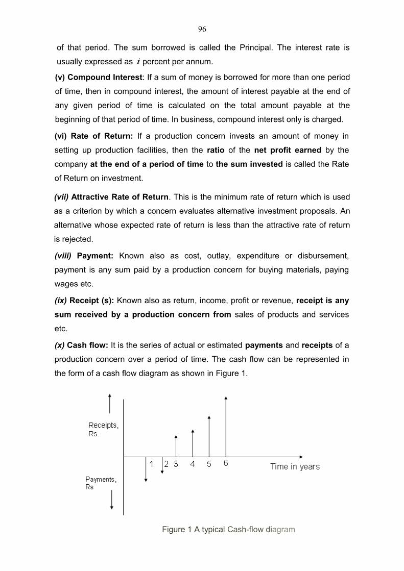
of that period. The sum borrowed is called the Principal. The interest rate is
usually expressed as i percent per annum.
(v) Compound Interest: If a sum of money is borrowed for more than one period
of time, then in compound interest, the amount of interest payable at the end of
any given period of time is calculated on the total amount payable at the
beginning of that period of time. In business, compound interest only is charged.
(vi) Rate of Return: If a production concern invests an amount of money in
setting up production facilities, then the ratio of the net profit earned by the
company at the end of a period of time to the sum invested is called the Rate
of Return on investment.
(vii) Attractive Rate of Return. This is the minimum rate of return which is used
as a criterion by which a concern evaluates alternative investment proposals. An
alternative whose expected rate of return is less than the attractive rate of return
is rejected.
(viii) Payment: Known also as cost, outlay, expenditure or disbursement,
payment is any sum paid by a production concern for buying materials, paying
wages etc.
(ix) Receipt (s): Known also as return, income, profit or revenue, receipt is any
sum received by a production concern from sales of products and services
etc.
(x) Cash flow: It is the series of actual or estimated payments and receipts of a
production concern over a period of time. The cash flow can be represented in
the form of a cash flow diagram as shown in Figure 1.
Figure 1 A typical Cash-flow diagram
96
(xi) Sunk costs: Engineering economic analysis is concerned with making
choices between engineering alternatives. For this purpose all past payments or
receipts (called Sunk Costs) 'concerning the alternatives are irrelevant, and
are therefore ignored. (sunk = done for)
(xii) Opportunity Costs: If a company invests certain sum of money into a
certain venture (or proposal) with an element of risk, that sum is no longer
available for investing in any other alternative venture. The profits or returns
lost as a result of not investing in a particular alternative is called the
Opportunity Cost.
(xiii) Asset: An asset of a production concern is a valuable like land, building,
machine, material etc. owned by the concern.
(xiv) Life of an Asset: The life of an asset can be considered in three ways,
(a) Actual or Technological Life of an asset is the duration during which it can
fulfill its required functions. It is determined from technological considerations. (b)
Accounting Life of an asset is the duration during which the investment made
in acquiring the asset is to be recovered from gross profits in the form of
depreciation.
(c) Economic life of an asset is the duration during which an asset performs its
technological function economically. The asset is actually used by the production
concern during its economic life only.
(xv) Depreciation: A company invests in assets expecting to earn profits by
making use of those assets. However, net profits would accrue only after the
investment made in acquiring the assets is recovered. Depreciation is systematic
procedure of recovering every year a portion of investment made on an asset
during its accounting life. Income tax during a year is chargeable only on the net
profit obtained by deducting the amount of depreciation from gross profits.
(xvi) Book Value of an Asset: At any time during the accounting life of an
asset, its book value is equal to its cost price minus the total amount of
depreciation charged on it by that time.
(xvii) Salvage Value: It is the actual or estimated value of an existing asset at
which it can be sold now or at a certain date in the future.
97

(xx) Retirement: It is the disposal of an existing asset through sales or
abandonment as scrap.
(xviii) Replacement: It means acquiring a new asset through purchase or lease
to perform the same or extended service which had so far been performed by
another asset which has been retired.
(xix) Defender and Challenger: When an economic analysis
is made to decide whether or not to replace an existing asset with another, the
existing asset is referred to as the Defender and the proposed replacement as the
Challenger.
98
LECTURE NO. 23
METHODS OF ECONOMIC EVALUATION OF ENGINEERING ALTERNATIVES
1. UNDISCOUNTED CASH FLOW METHODS -PAY BACK PERIOD METHOD
2. DISCOUNTED CASH FLOW METHODS
A) NET PRESENT VALUE METHOD
B) EQUIVALENT ANNUAL METHOD
C) RATE OF RETURN METHOD
3. COST- BENEFIT ANALYSIS, SOCIAL COSTS, SOCIAL BENEFITS
Methods of Economic Evaluation of Engineering Alternatives
There are basically two kinds of methods of economic evaluation of
engineering alternatives,
1. Undiscounted Cash Flow Methods and
2. Discounted Cash Flow Methods.
1. Undiscounted Cash Flow Methods: In such methods future payments and
receipts are not discounted. In other words: the discount rate is considered as
zero. Because in most business world, interest is charged, these methods must
be considered only as approximate and rough. However, because of their
simplicity they are often used as a first screening of alternatives before applying
the discounted cash flow methods. The most popular undiscounted
cash-flow method is the Pay-back Period method.
Pay-back Period Method. In this method, the time period during which the
undiscounted future profits will just equal the original investment is calculated.
That alternative is considered to be the best corresponding to which the payback
period is the smallest.
2. Discounted Cash Flow Methods. In these methods, future payments and
receipts are discounted. In other words these methods take into account the time
value of money. There are three methods belonging to this category. However, all
the three methods are equivalent and provide identical evaluation if investments in
the various alternatives under consideration are equal.
(A) Net Present Value Method : This is also known as the Net Present Worth
method. In this method, we find the net present worth (value) of all estimated
receipts and payments associated with a given alternative using a discount rate
equal to what the company considers an attractive rate of return. If the net present
99
value of an alternative is positive, it means that the likely rate of return obtainable
from the given alternative is greater than the attractive rate of return or vice-versa.
That alternative is considered the best whose net present value is algebraically
the
maximum.
(B) Equivalent Annual Cost Method: In this method, the equivalent annual cost
of each alternative cash flow is calculated. The equivalent annual cost of a given
cash flow is that uniform series of end-of-year payments whose net present value
is equal to the net present value of all the payments (and receipts) of the given
ash flow, using a given attractive rate of return. That alternative is considered as
the best whose equivalent annual cost is the smallest.
(C) Rate of Return Method: In this method, the expected rates of return of the
various alternatives are calculated. That alternative is the best whose expected
rate of return is the largest. To find the rate of return, it is usual to adopt a trial and
error procedure. In this procedure, the net present value of the given alternative is
calculated using a particular assumed value of discount rate. If the net present
value is positive, it means that the expected rate of return is larger than the
assumed discount rate, and vice-versa. Accordingly in the next trial, a larger
discount rate is used if the previous net present value was positive, and vice-
versa. The procedure is terminated when the net present value is sufficiently
small.
Cost-Benefit Analysis
This is employed for calculating feasibility of engineering alternatives of large
government projects, for example, setting up new steel plants, airports, nuclear or
thermal power stations etc. In such projects, it is necessary to consider social
instead of purely financial criteria. During cost-benefit analysis, that alternative is
selected which is expected either
(a) to result in the largest net social benefit based on a given social rate of
return (usually small) which is given by
Net social benefit =
Present worth of all social benefits - Present worth of all social costs
100
or (b) to provide the largest rate of return considering the value
of all social benefits and all social costs.
Social Costs: They include not only the cost of direct investments made by the
government but also costs incurred by every affected member of the community.
For example, if there are specific alternative sites being evaluated for setting up a
steel plant, not only the costs of land, buildings, equipment, roads and railway
lines are relevant, but also the cost of displacement, rehabilitation and hardship of
families whose homes and farms have to be requisitioned, and costs of ecological
deterioration caused by large scale human encroachment--for example, loss of
wild life and picnic spots etc.
Social Benefits: The benefits include not only the revenues accruing to the
government but also to all direct and indirect beneficiaries in the community as a
whole. For example, the benefits of a steel plant include not only the income from
sales of steel and steel products, but also increased employment to the
local community, growth of ancillary industry, improvement of rail, road and
communications, and modernization of the community etc.
Procedure:
(i) Identify the various project alternatives. Then for each proposal, carry out the
following steps.
(ii) Identify all categories of relevant social benefits and social costs which may be
expected to result from the proposal. Ideally the costs and benefits should be all
inclusive, i.e. every possible cost and benefit should be found for every possible
member of the community. However, practicability limits the numbers of persons
considered.
(iii) Evaluate each item of cost and benefit on a common scale, usually money.
The estimates of costs and benefits should be prepared for each year of the
project’s economic life.
(iv) Prepare a cash flow diagram based on the above estimates and calculate the
net social benefit using a social rate of return, or preferably the expected rate of
return.
(v) The alternative that yields the largest net social benefit or the largest expected
rate of return is the best.
101

102
LECTURE NO. 24
PROCESS SCHEDULING
Scheduling is an important tool for manufacturing and engineering, where
it can have a major impact on the productivity of a process. In manufacturing, the
purpose of scheduling is to minimize the production time and costs, by telling a
production facility when to make, with which staff, and on which equipment.
Production scheduling aims to maximize the efficiency of the operation and
reduce costs.
Production scheduling tools greatly outperform older manual scheduling
methods.
Companies use backward and forward scheduling to allocate plant and
machinery resources, plan human resources, plan production processes and
purchase materials.
Forward scheduling is planning the tasks from the date resources become
available to determine the shipping date or the due date.
Backward scheduling is planning the tasks from the due date or required-
by date to determine the start date and/or any changes in capacity required.
The benefits of production scheduling include:
• Process change-over reduction
• Inventory reduction, leveling
• Reduced scheduling effort
• Increased production efficiency
• Labor load leveling
• Accurate delivery date quotes
• Real time information
Productivity
Productivity is the relation between quantity of inputs and quantity of
output.
103
Inputs
Inputs are plant, labor, materials, tooling, energy and a clean environment.
Outputs
Outputs are the products produced in factories either for other factories or
for the end buyer. The extent to which any one product is produced within any one
factory is governed by transaction cost.
Within the factory
The output of any one work area within the factory is an input to the next
work area in that factory according to the manufacturing process. For example the
output of the cutting room is an input to the sewing room.
For the next factoryBy way of example, the output of a paper mill is an input to a print factory.
The output of a petrochemicals plant is an input to an asphalt plant, a cosmetics
factory and a plastics factory.
For the end buyer
Factory output goes to the consumer via a service business such as a
retailer or an asphalt paving company.
Resource allocation
Resource allocation is assigning inputs to produce output. The aim is to
maximize output with given inputs or to minimize quantity of inputs to produce
required output.
Scheduling Algorithms
Production scheduling can take a significant amount of computing power if
there are a large number of tasks. Therefore a range of short-cut algorithms
(heuristics) (also known as dispatching rules) are used:
Stochastic Algorithms
• Economic Lot Scheduling Problem
• Economic production quantity
104

Heuristic Algorithms
• Modified due date scheduling heuristic
• Shifting bottleneck heuristic
105
LECTURE NO. 25
LINEAR PROGRAMMING: INTRODUCTION, SALIENT FEATURES OF LINEAR
PROGRAMMING (TERMINOLOGY)
Definition of Operations Research
The Operational Research Society of India:
Operations Research is the attack of modern science on complex problems
arising in the direction and management of large systems of men, machines,
materials and money in industry, business, government and defense.
A classical definition of Operations Research (Ackoff and Arnoff):
Operations Research is the application of scientific methods, techniques
and tools to problems involving the operations of systems so as to provide those
in control of the system with optimum solutions to the problem".
Characteristics or Significant Features of Operations Research
The significant features of operations research can be stated as:
1. Decision Making Tool
2. Scientific Approach.
3. Inter-disciplinary Team Approach
4. System Approach
5. Operations Research largely depends on Digital Computer.
6. Objective.
MODELS IN OPERATIONS RESEARCH
Operations research expresses a problem by a model: A model is a
theoretical abstraction (approximation) of a real-life problem. It can also be
defined as a simplified representation of an operations or a process in which only
the basic aspects or the most important features of a typical problem under
investigation are considered. The object of the models is to provide means for
analyzing the behavior of the system for the purpose of improving its
performance.
TECHNIQUES USED IN OPERATIONS RESEARCH
1. Linear Programming. It is used in the solution of problems concerned with
assignment of personnel, blending of materials, transportation and distribution,
facility planning, media selection, product mix etc.
106
2. Dynamic Programming.
3. Queueing Theory. It is used in solving problems concerned with traffic
congestion,
servicing machines subject to breakdown, air traffic scheduling, production
scheduling, determining optimum number of repairment for a group of machines.
4. Inventory theory
5. CPM and PERT Techniques.
6. Game Theory (Competitive Models).
7. Replacement Models.
8. Sequencing Models
9. Decision Analysis Models.
10. Simulation.
INTRODUCTION to Linear Programming
Linear programming is one of the operations research techniques. It has its
early use for military applications but it is employed widely for business problems.
Definition:
Linear programming is a mathematical technique for the purpose of
allocating the limited resources in an optimum manner (i.e., either maximum or
minimum) to achieve the objectives of the business, which may be maximum
overall profit or minimum overall cost. The word "linear" means that the
relationships handled are those which can be represented by straight lines, i.e.,
the relationships are of the form y = ax + b and the word "programming" means
"taking decisions systematically".
In other words, linear programming is the optimization (either maximization
or
minimization) of a linear function of variables subject to constraint of linear
inequalities.
Thus, linear programming involves the planning of activities to obtain an
"optimal" result i.e., a result that reaches the specified goal best (according to the
mathematical model) among all feasible alternatives.
(i) It attempts to maximize .or minimize a linear function of decision
variables.
107
(ii) The values of the decision variables are selected in such a way that they
satisfy a set of constraints, which are in the form of linear inequality.
SALIENT FEATURES OF LINEAR PROGRAMMING (TERMINOLOGY)
Linear programming is based on the following basic concepts:
1. Decision Variables (Activities). Decision variables are the variables whose
quantitative values are to be found from the solution of the model so as to
minimize or maximize the objective function. For example, decision variables in a
product mix manufacturing, represents the quantities of the different products to
be manufactured by using its limited resources, such as men, machines,
materials, money etc. The decision variables are usually denoted by x1, x2,
……,xn.
2. Objective Functions. It states the determinants of the quantity either to be
maximized or to be minimized. For instance, profit is a function to be maximized
or cost is a function to be minimized. An objective function must include all the
possibilities with profit or cost coefficient per unit of output. For example, for a firm
which produces four different products A, B, C and D in
quantities Q1 , Q2, Q3 and Q4 respectively, the objective function can be stated as
:
Minimise C = QI CI + Q2 C2 + Q3 C3 + Q4 C4,
where C is the total cost of production, and C1, C2, C3 and C4 are unit costs of
products A, B, C and D respectively.
3. Constraints (Inequalities). These are the restrictions imposed on decision
variables. These may be in terms of availability of raw materials, machine hours,
man hours etc. Suppose each of the above items A, B, C and D requires tl, t2, t3
and t4 machine hours respectively. The total machine hours are T hours, and this
is a constraint.
Therefore it can be expressed as:
Q1 t1 + Q2 t2 + Q3 t3 + Q4 t4 ≤ T
4. Non-Negative Condition. The linear programming model essentially seeks
that the values for each variable can either be zero or positive. In no case it can
be negative. For the products A, B, C and D the non-negative conditions can be :
Q1 ≥ 0 t1 ≥0Q2 ≥ 0 t2 ≥0Q3 ≥ 0 and also t3 ≥0Q4 ≥ 0 t4 ≥0
108
This implies that quantity produced can be at the most zero and not below
that. Similarly, the machine hours expended for each unit A, B, C and D can be at
the most zero and in no case it can be negative.
5. Linear Relationship. It implies straight line or proportional relationship among
the
relevant variables. It means change in one variable produces proportionate
change in other variables.
6. Process and its Level. Process represents to produce a particular output. If a
product can be produced in two different ways, then there are two different
processes or decision variables for the purpose of linear programming.
7. Feasible Solution. All such solutions which can be worked out under given
constraints are called "feasible solutions" and region comprising such solution is
called the "feasible region".
8. Optimum Solution. Optimum means either maximum or minimum. The object
of
obtaining the feasible optimum solution may be maximization of profit or
minimization of cost. Optimum solution is the best of all feasible solutions.
109
LECTURE NO. 26
FORMULATION OF LINEAR PROGRAMMING MODEL, ADVANTAGES,
LIMITATIONS AND APPLICATIONS OF LINEAR PROGRAMMING, SOLUTION
OF LINEAR PROGRAMMING PROBLEMS.
Formulation of LP Model. Formulation of LP model refers to translating a
problem into a format of mathematical equation.
Assumptions in Linear Programming
(i) There is a well defined objective function such as maximizing profit or
minimizing cost.
(ii) There are a number of restrictions or constraints (on the amount and extent of
available resources for satisfying the objective function) which can be expressed
in
quantitative terms. These may refer to man-hours, machine hours, raw materials,
storage space, capital etc.
(iii) The parameters are subject to variation in magnitude.
(iv)The relationship expressed by constraints and the objective function are linear.
(v) The objective function is to be optimized w.r.t. the decision variables involved
in the phenomenon. The decision variables are non-negative and represent
real life situation.
Advantages, Limitations and Applications of Linear Programming
Advantages:
(i) Linear programming helps the management to make effective utilization of
limited
production resources.
(ii) Linear programming improves the quality of decision making by replacing
rules of thumb.
(iii) It provides feasibility in analyzing a variety of multi-dimensional problems.
(iv) It highlights the bottlenecks in the production processes.
(v) It helps in re-evaluation of the basic plan to meet changing conditions in the
business (e.g., sales, demand etc.).
110
Limitations:
(i) The assumptions that all relations are linear may not hold good in many real
situations.
(ii) In linear programming all coefficients and constraints are stated with certainty.
(iii) The solution many times is in fractions which may not remain optimal when
rounded-off. .
(iv) When the number of variables or constraints involved are quite large then it be
com necessary to use computers.
(v) It deals with only a single objective problems, whereas in real life situations
there
may be more than one conflicting objectives.
Applications: Some of the applications of linear programming in industry,
business, and other fields are as follows:
1. Product Mix. A company can produce several different products, each of
which
requires the use of limited resources. Linear programming helps to determine
the
quantity of each product to be manufactured in order to maximize profit.
2. Production Planning. Linear programming helps in production planning
(inventory control, manpower, equipment selection, etc.) in order to minimize
total operations costs.
3. Assembly line Balancing. Linear programming techniques help to minimize.
tot
elapse time in assembly process.
4. Blending Problem. When a product can be made from a variety of available
raw
materials, each of which has a particular composition and price, linear
programming technique is used to determine minimum cost blend.
5. Media Selection. Linear programming helps in determining the advertising
media
mix so as to maximize the effective exposure at minimum cost.
6. Traveling Salesman Problem
7. Physical Distribution. It helps in selecting most economical and effective
location for the manufacturing plant and distribution centers.
111
8. Staffing Problem. Linear programming helps to allocate optimum manpower to
a
particular job so as to minimize total over time cost and total manpower.
9. Job Evaluation and Selection. Selection of suitable person for a specified job
and
evaluation of job in organization has been done with the help of linear
programming.
10. Agriculture. To allocate limited resources such as land, labour, water supply and
working capital etc. in the way so as to improve productivity.
11. Military. Military applications include the problem of selecting an effective air
weapon -system against enemy.
12. Routing Problem. To determine the most economic pattern and timings for
flights so as to make the most efficient use of aircraft and crews.
Solution of Linear Programming Problems
Linear Programming Problems can be solved by following methods:
1. Graphical method
2. simplex method
3. Transportation method
4. Assignment models
The graphical method can be used only for two or three variables; where
as the other methods can be used for any number of variables.
Illustrative Problems on Formulation of Linear Programming Model
Example: The manager of an oil refinery must decide on the optimal mix of two
possible blending processes of which the input and output per production run are
given as follows:
Process Input (units) Output
Crude A Crude B Gasoline X Gasoline Y
1 5 3 5 8 2 4 5 4 4
The maximum amount available of crude A and B are 200 units and 150
units, respectively. Market requirements show that at least 100 units of gasoline X
and 80 units of gasoline Y must be produced. Formulate this problem as an linear
112
programming model to maximize profit. The profit per production run
from process 1 and process 2 are Rs. 300 and Rs. 400, respectively.
Linear Programming Model Formulation:
Let,
Decision variables
x1 = number of units of Gasoline from process 1
x2 = number of units of Gasoline from process 2
Objective function, Maximize z =300 x1 + 400 x2
Subject to constraints:
5x1 + 4x2 ≤
200
3x1 + 5x2 ≤
150
5x1 + 4x2 ≤100
8x1+ 4x2 ≤ 80
x1 ≥ 0 and x2 ≥0
113
LECTURE NO. 27
QUEUING THEORY: INTRODUCTION, ELEMENTS OF QUEUING SYSTEM, 1)
INPUT SOURCE, 2) QUEUE
Queuing Theory (Waiting Lines)
INTRODUCTION
The formation of queues or waiting lines is a most common phenomenon in
our every day life. It occurs where the current demand exceeds the current
capacity to provide that service.
Queues are also formed even when the service rate is higher than the arrival
rate due to random pattern of arrival of customers. The examples of the places
where the queues may be formed are barber's shop, ration shop, cinema ticket
window, bus stop, bank counters, railway reservation counters, telephone booth,
doctor’s clinic, repair shops, automobile service centers etc.
Besides these, queues are also formed in manufacturing industry in
situations where in-process goods waits for next operation, or waits for getting
moved to another place, machine waiting for repair parts or components waiting
for assembly in assembly lines, blunt tools waiting for reground, workers waiting at
the tool crib to obtain tools etc. This may increase production cycle duration which
adds to the cost of the product and it may also delay the specified delivery period.
Queues may not be a physical line of customers; it may be merely a list of
customers, units, orders etc. Some specified examples of such type of queues
are: unconnected telephone calls waiting list of passengers for a berth etc.
The most important issue in waiting line problems is to decide the best level
of service the organization should provide. Providing too much service would
involve excessive cost on the other hand inadequate service capacity would
result in long waiting lines which results in dissatisfaction of customers or
sometimes loss of customers. Thus the ultimate goal is to achieve an economic
balance between the cost of service and the cost associated with waiting for
that service.
Queueing theory provides a large number of alternative mathematical
models for describing and solving waiting line problems.
114
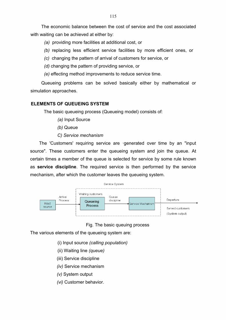
The economic balance between the cost of service and the cost associated
with waiting can be achieved at either by:
(a) providing more facilities at additional cost, or
(b) replacing less efficient service facilities by more efficient ones, or
(c) changing the pattern of arrival of customers for service, or
(d) changing the pattern of providing service, or
(e) effecting method improvements to reduce service time.
Queueing problems can be solved basically either by mathematical or
simulation approaches.
ELEMENTS OF QUEUEING SYSTEM
The basic queueing process (Queueing model) consists of:
(a) Input Source
(b) Queue
C) Service mechanism
The 'Customers' requiring service are ·generated over time by an "input
source". These customers enter the queueing system and join the queue. At
certain times a member of the queue is selected for service by some rule known
as service discipline. The required service is then performed by the service
mechanism, after which the customer leaves the queueing system.
Fig. The basic queuing process
The various elements of the queueing system are:
(i) Input source (calling population)
(ii) Waiting line (queue)
(iii) Service discipline
(iv) Service mechanism
(v) System output
(vi) Customer behavior.
115
1. Input source
Two important characteristics of the input source are:
(i) its size and (ii) the pattern of arrival.
The size is the total number of customers that might require service from
time to time. The size of the input source is generally assumed to be infinite. The
railway reservation system, tax / toll both on highway etc. are the example of
infinite queue.
The arrival of the customers may be either at a constant rate or at random.
Most arrivals in a service system are at random. This is when each arrival is
independent of its previous arrivals. The exact prediction of any arrival in random
system is not possible. Therefore, the number of arrivals per unit time (rate of
arrival) is estimated by Poisson distribution.
2. Queue
A queue is characterized by the maximum permissible number of
customers that it contains. Units requiring service enter the system and join a
queue. In some service systems only a limited number of customers are allowed
in the system and new arrivals are not allowed to join the system unless the
number becomes less than the limiting value.
116
LECTURE NO. 28
QUEUING THEORY: CHARACTERISTICS OF WAITING LINES, SERVICE
DISCIPLINE, SERVICE MECHANISM, SYSTEM OUT PUT, CUSTOMER
BEHAVIOR.
CHARACTERISTICS OF WAITING LINES
The important characteristics required to study the waiting line are:
(i) Waiting time: It is the time that a customer spends in the queue before being
taken up for service.
(ii) Service time: It is the time period between two successive services. It may be
either constant or variable.
(iii) Waiting time in the system: It implies the time spent by the Customer in the
queue system.
Waiting time in the system = Waiting time + Service time
(iv) Queue length: It implies the number of customers waiting in the queue.
(v) System length: System length is equal to the number of customers in the
queue plus those being served.
SERVICE DISCIPLINE
It refers to the order in which the customers waiting in queue are selected for
service. It may be first-come-first-served, random or according to some priority
procedure. The rules governing order of service may be.
(i) FIFO. First-In-First-Out. (i.e., first-come-first-served)
According to FIFO, the customers are served in the order of their arrival.
Examples are bank counters, railway reservation counters etc.
(ii) LIFO. Last-In-First-Out. According to LIFO, the items arriving last are taken out
first. Example, in big godowns the items arrived last are taken out first.
(iii) SIRO. Service In Random Order. (or Random and priority) Sometimes, certain
customers are given priority for service i.e., the arriving customer is chosen for
service ahead of some other customers already in the queue. Example: Serious
patients are given priority for treatment, vital machines are attended to first in the
117
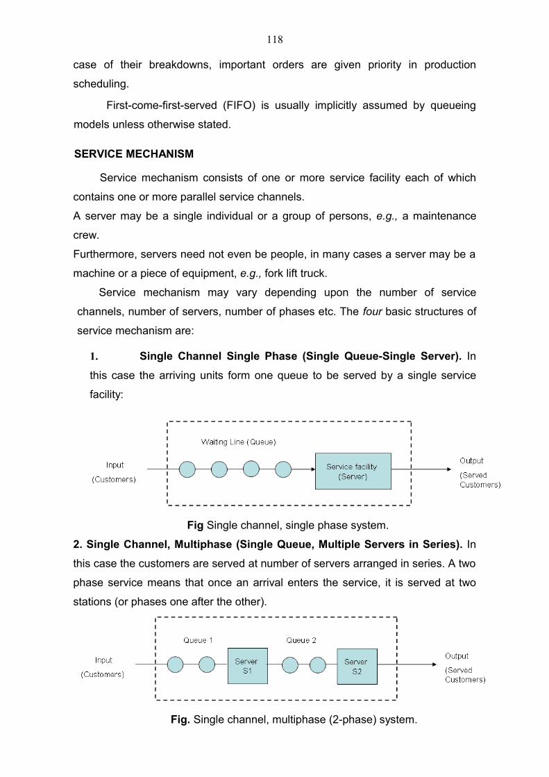
case of their breakdowns, important orders are given priority in production
scheduling.
First-come-first-served (FIFO) is usually implicitly assumed by queueing
models unless otherwise stated.
SERVICE MECHANISM
Service mechanism consists of one or more service facility each of which
contains one or more parallel service channels.
A server may be a single individual or a group of persons, e.g., a maintenance
crew.
Furthermore, servers need not even be people, in many cases a server may be a
machine or a piece of equipment, e.g., fork lift truck.
Service mechanism may vary depending upon the number of service
channels, number of servers, number of phases etc. The four basic structures of
service mechanism are:
1. Single Channel Single Phase (Single Queue-Single Server). In
this case the arriving units form one queue to be served by a single service
facility:
Fig Single channel, single phase system.
2. Single Channel, Multiphase (Single Queue, Multiple Servers in Series). In
this case the customers are served at number of servers arranged in series. A two
phase service means that once an arrival enters the service, it is served at two
stations (or phases one after the other).
Fig. Single channel, multiphase (2-phase) system.
118
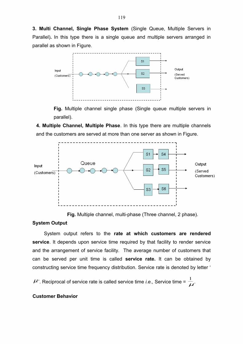
3. Multi Channel, Single Phase System (Single Queue, Multiple Servers in
Parallel). In this type there is a single queue and multiple servers arranged in
parallel as shown in Figure.
Fig. Multiple channel single phase (Single queue multiple servers in
parallel).
4. Multiple Channel, Multiple Phase. In this type there are multiple channels
and the customers are served at more than one server as shown in Figure.
Fig. Multiple channel, multi-phase (Three channel, 2 phase).
System Output
System output refers to the rate at which customers are rendered
service. It depends upon service time required by that facility to render service
and the arrangement of service facility. The average number of customers that
can be served per unit time is called service rate. It can be obtained by
constructing service time frequency distribution. Service rate is denoted by letter ‘
µ ’. Reciprocal of service rate is called service time i.e., Service time = µ1
.
Customer Behavior
119
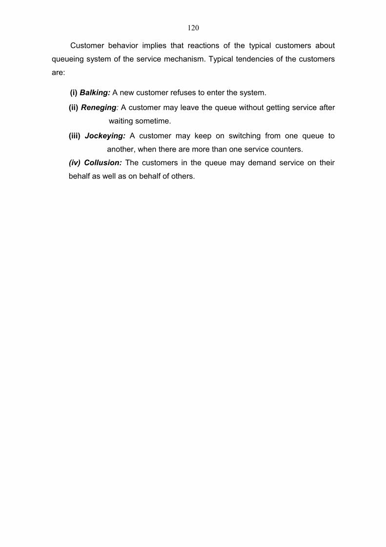
Customer behavior implies that reactions of the typical customers about
queueing system of the service mechanism. Typical tendencies of the customers
are:
(i) Balking: A new customer refuses to enter the system.
(ii) Reneging: A customer may leave the queue without getting service after
waiting sometime.
(iii) Jockeying: A customer may keep on switching from one queue to
another, when there are more than one service counters.
(iv) Collusion: The customers in the queue may demand service on their
behalf as well as on behalf of others.
120
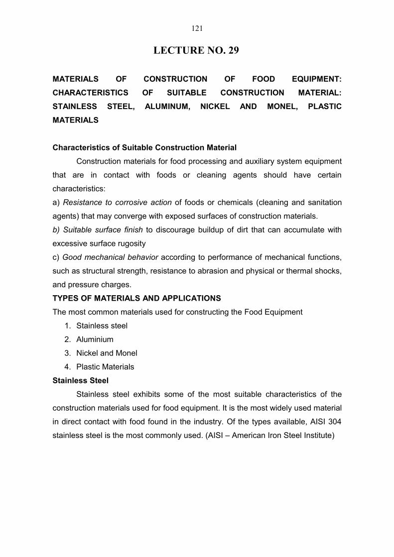
LECTURE NO. 29
MATERIALS OF CONSTRUCTION OF FOOD EQUIPMENT:
CHARACTERISTICS OF SUITABLE CONSTRUCTION MATERIAL:
STAINLESS STEEL, ALUMINUM, NICKEL AND MONEL, PLASTIC
MATERIALS
Characteristics of Suitable Construction Material
Construction materials for food processing and auxiliary system equipment
that are in contact with foods or cleaning agents should have certain
characteristics:
a) Resistance to corrosive action of foods or chemicals (cleaning and sanitation
agents) that may converge with exposed surfaces of construction materials.
b) Suitable surface finish to discourage buildup of dirt that can accumulate with
excessive surface rugosity
c) Good mechanical behavior according to performance of mechanical functions,
such as structural strength, resistance to abrasion and physical or thermal shocks,
and pressure charges.
TYPES OF MATERIALS AND APPLICATIONS
The most common materials used for constructing the Food Equipment
1. Stainless steel
2. Aluminium
3. Nickel and Monel
4. Plastic Materials
Stainless Steel
Stainless steel exhibits some of the most suitable characteristics of the
construction materials used for food equipment. It is the most widely used material
in direct contact with food found in the industry. Of the types available, AISI 304
stainless steel is the most commonly used. (AISI – American Iron Steel Institute)
121
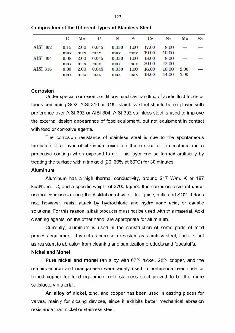
Composition of the Different Types of Stainless Steel
CorrosionUnder special corrosion conditions, such as handling of acidic fluid foods or
foods containing SO2, AISI 316 or 316L stainless steel should be employed with
preference over AISI 302 or AISI 304. AISI 302 stainless steel is used to improve
the external design appearance of food equipment, but not equipment in contact
with food or corrosive agents.
The corrosion resistance of stainless steel is due to the spontaneous
formation of a layer of chromium oxide on the surface of the material (as a
protective coating) when exposed to air. This layer can be formed artificially by
treating the surface with nitric acid (20–30% at 60°C) for 30 minutes.
Aluminum
Aluminum has a high thermal conductivity, around 217 W/m. K or 187
kcal/h. m. °C, and a specific weight of 2700 kg/m3. It is corrosion resistant under
normal conditions during the distillation of water, fruit juice, milk, and SO2. It does
not, however, resist attack by hydrochloric and hydrofluoric acid, or caustic
solutions. For this reason, alkali products must not be used with this material. Acid
cleaning agents, on the other hand, are appropriate for aluminum.
Currently, aluminum is used in the construction of some parts of food
process equipment. It is not as corrosion resistant as stainless steel, and it is not
as resistant to abrasion from cleaning and sanitization products and foodstuffs.
Nickel and Monel
Pure nickel and monel (an alloy with 67% nickel, 28% copper, and the
remainder iron and manganese) were widely used in preference over nude or
tinned copper for food equipment until stainless steel proved to be the more
satisfactory material.
An alloy of nickel, zinc, and copper has been used in casting pieces for
valves, mainly for closing devices, since it exhibits better mechanical abrasion
resistance than nickel or stainless steel.
122
Monel is the preferred material for common salt processing systems since
it exhibits even better corrosion resistance than stainless steel. It is also employed
in pumps that handle alcohol, brines, vegetal oils, and fruit juices.
Plastic Materials
Plastic materials are used in harvesting and transporting agricultural raw
materials to the food processing plant, in food packaging of solid and liquid foods,
and even in food process equipment (mainly processing tanks).
The most important plastics are:
• Polypropylene.• High density polyethylene• Rigid PVC• Polyester• Epoxy resins
123
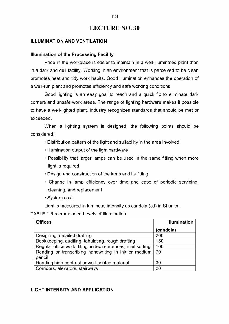
LECTURE NO. 30
ILLUMINATION AND VENTILATION
Illumination of the Processing Facility
Pride in the workplace is easier to maintain in a well-illuminated plant than
in a dark and dull facility. Working in an environment that is perceived to be clean
promotes neat and tidy work habits. Good illumination enhances the operation of
a well-run plant and promotes efficiency and safe working conditions.
Good lighting is an easy goal to reach and a quick fix to eliminate dark
corners and unsafe work areas. The range of lighting hardware makes it possible
to have a well-lighted plant. Industry recognizes standards that should be met or
exceeded.
When a lighting system is designed, the following points should be
considered:
• Distribution pattern of the light and suitability in the area involved
• Illumination output of the light hardware
• Possibility that larger lamps can be used in the same fitting when more
light is required
• Design and construction of the lamp and its fitting
• Change in lamp efficiency over time and ease of periodic servicing,
cleaning, and replacement
• System cost
Light is measured in luminous intensity as candela (cd) in SI units.
TABLE 1 Recommended Levels of Illumination
Offices Illumination
(candela)Designing, detailed drafting 200Bookkeeping, auditing, tabulating, rough drafting 150Regular office work, filing, index references, mail sorting 100Reading or transcribing handwriting in ink or medium pencil
70
Reading high-contrast or well-printed material 30Corridors, elevators, stairways 20
LIGHT INTENSITY AND APPLICATION
124
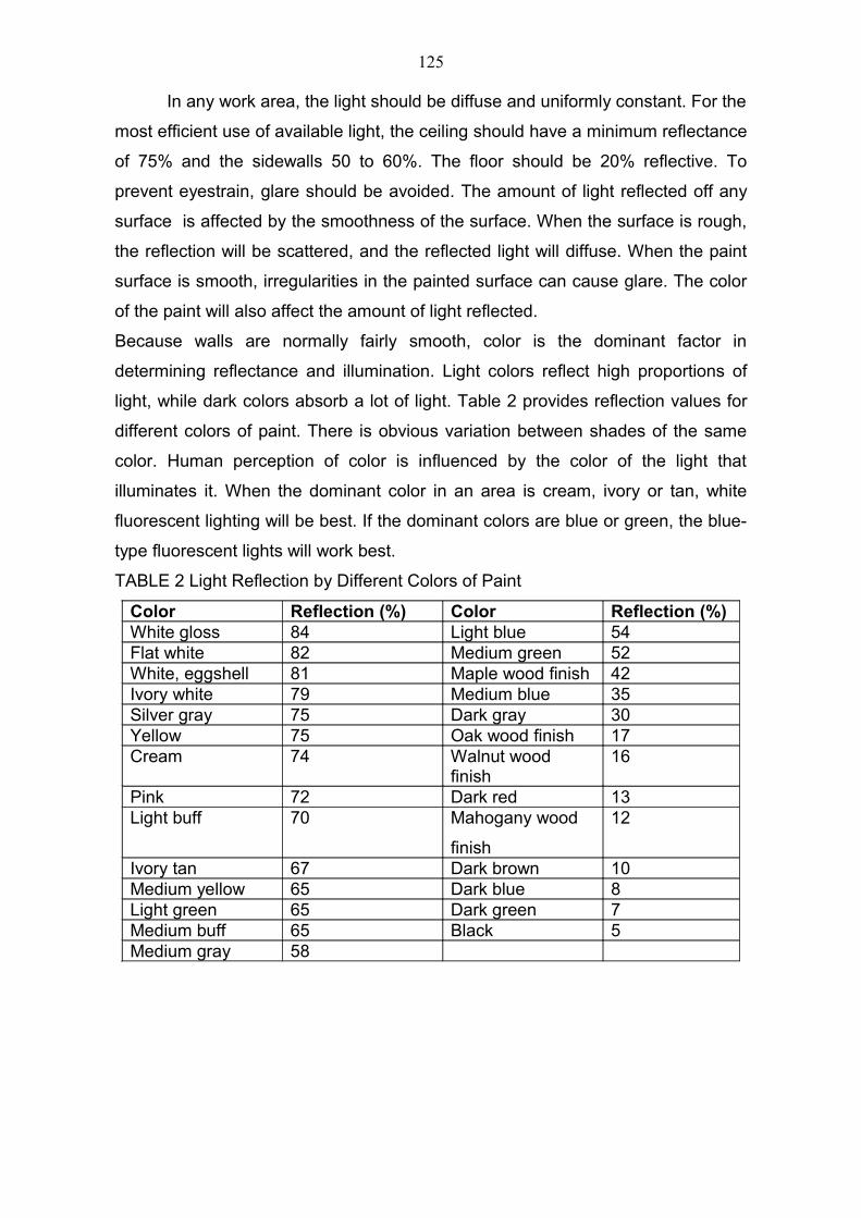
In any work area, the light should be diffuse and uniformly constant. For the
most efficient use of available light, the ceiling should have a minimum reflectance
of 75% and the sidewalls 50 to 60%. The floor should be 20% reflective. To
prevent eyestrain, glare should be avoided. The amount of light reflected off any
surface is affected by the smoothness of the surface. When the surface is rough,
the reflection will be scattered, and the reflected light will diffuse. When the paint
surface is smooth, irregularities in the painted surface can cause glare. The color
of the paint will also affect the amount of light reflected.
Because walls are normally fairly smooth, color is the dominant factor in
determining reflectance and illumination. Light colors reflect high proportions of
light, while dark colors absorb a lot of light. Table 2 provides reflection values for
different colors of paint. There is obvious variation between shades of the same
color. Human perception of color is influenced by the color of the light that
illuminates it. When the dominant color in an area is cream, ivory or tan, white
fluorescent lighting will be best. If the dominant colors are blue or green, the blue-
type fluorescent lights will work best.
TABLE 2 Light Reflection by Different Colors of Paint
Color Reflection (%) Color Reflection (%)White gloss 84 Light blue 54Flat white 82 Medium green 52White, eggshell 81 Maple wood finish 42Ivory white 79 Medium blue 35Silver gray 75 Dark gray 30Yellow 75 Oak wood finish 17Cream 74 Walnut wood
finish16
Pink 72 Dark red 13Light buff 70 Mahogany wood
finish
12
Ivory tan 67 Dark brown 10Medium yellow 65 Dark blue 8Light green 65 Dark green 7Medium buff 65 Black 5Medium gray 58
125
TYPES OF LAMPS
Many types of lamps are used in processing areas. In most cases,
fluorescent lamps are favored because they have about 2.5 times the efficiency of
incandescent lamps. They also give soft diffused light without glare. Fluorescent
lamps are best suited in areas where the lamp stays on for long periods of time. In
places where lamps are frequently switched on and off, fluorescent light should
not be used. Frequent on and off service not only results in a short lifespan of the
lighting element but places an extra load on the starting transformer. Fluorescent
lamps can be used for about 2500 to 4000 h before they need to be replaced.
Incandescent lamps must be replaced every 800 to 1000 h.
Most installations use fluorescent lighting in all areas possible. In some
high moisture areas, including cold rooms and where explosive vapors may be
present, incandescent light fittings with vapor-proof fixtures are required. In the
cereal industry, cereal dust can be very explosive when mixed with the right
amount of air. In these cases, light bulbs and all fittings are completely enclosed
and water tight.
At loading docks, large warehouses and outside areas, where extensive
coverage is required, mercury vapor lamps are used. Mercury vapor lamps are
several times more efficient than fluorescent lighting.
Incandescent lamps radiate more long-wave radiation in the yellow and red
ranges, while fluorescent lighting is bluer. Incandescent lamps produce light and
heat. This is an obvious drawback in cold storage areas. If fluorescent lighting is
used in cold rooms, the tubes must be rated to operate at temperatures below
5ºC.
The installation cost for fluorescent lighting is considerably greater than the
cost for incandescent lighting. The energy savings will pay for this additional
expense over time. All light bulbs should be replaced at regular intervals.
Replacing them only if they are broken means that there will be one or two lights
out at any given time. Lights have an average lifespan and should be replaced
before they break.
VENTILATION
Ventilation is the supply of fresh, conditioned air to replace unwanted air.
Conditioning can include alteration of moisture content, change of temperature,
and filtering to remove particulates and organisms.
126
Within the processing area, ventilation will remove obnoxious odors,
moisture, and heat and replace it with air that is free from contaminants and air
that will increase the comfort level of workers. The amount of air is calculated as a
replacement volume. Depending upon the production processes, the air can be
replaced from 6 to 20 times per hour. It is also advisable to keep the processing
area under a slight positive pressure. This will ensure that processing area air
flows out when a door is opened.
Special air is required in areas where baby formula is handled or where
aseptic operations take place. In these cases, air will be filtered through special
filters that will remove organisms. The processing area must be under positive
pressure at all times so that no organisms can enter from adjacent processing
areas.
127
LECTURE NO. 31
CLEANING & SANITIZATION
Cleaning and sanitation should be considered an integral part of food
process design and food processing operations. The food processing equipment
should be designed to facilitate the removal and draining of all the process
effluents (steam condensate, waste solids, e.g., peels). All dead ends in tanks,
containers, and piping should be eliminated.
Fouling is particularly important in heat exchangers and other installations
involving fluid flow (evaporators, filters, cyclones, etc.). The food processing
equipment must be cleaned easily either by quick dismantling and cleaning the
parts, or by Cleaning-In-Place (CIP) techniques. The equipment of small food
processing plants is usually cleaned by periodic dismantling of the principal units,
such as pumps, plate heat exchangers, filters etc. Quick dismantling and re-
assembling of process piping is facilitated by various hand opening clumps.
The design and installation of CIP systems in large food processing plants
requires specialized experience in pipe flow, sanitation, processing operations,
and process control.
The CIP system involves the following sequential operations: 1) Pre-rinsing
with cold (soft) water; 2) alkali wash (supplemented with sodium hypochlorite); 3)
intermediate water rinse; 4) acid rinse; 5) final water rinse; and 6) rinse with
sanitizing solution (sodium hypochlorite) or flushing with hot (90 °C) water.
The CIP system is actually a chemical cleaning operation, in which the
chemical solution is brought into contact with all soiled surfaces. Addition of
surface active substances, reducing substantially the surface tension of water,
facilitates the penetration of water and aqueous cleaning solutions into crevices of
the equipment. The required tanks, pumps, pipes, valves and heaters (heat
exchangers or steam injection devices) are used either as single-use or re-use
(re-circulation) systems. Air-operated piston or diaphragm-type pumps are used to
feed the chemical solutions. For safety reasons, the pumps and the chemical
supply containers are enclosed in a separate compartment of the processing
plant.
Ball spray devices are used to clean process and storage tanks. Cylindrical
and rectangular tanks are cleaned using liquid feed rates of 8-12 L/min m2 internal
surface, while vertical silos require liquid rates of 25-35 L/min m tank
128
circumference. Adequate inclination (slope) of piping and process vessels is
essential for self-draining of process and cleaning liquids.
Usually, food equipment must be cleaned daily, after a processing period.
However, when different products are processed in the same equipment, cleaning
depends also on the frequency of product changes.
Effective CIP requires automation of the whole system. Microprocessor
controllers (PLC) are used in connection with on-line sensors for temperature,
level, flow rate, pressure, and valve position. The concentration of cleaning agents
and organic effluents can be measured with pH meters, redox potential meters,
and optical density meters. The degree of surface contamination can be
determined by pressure drop measurements in the pipeline.
Definition of SanitationThe word sanitation comes from the Latin word sanitas, which means
"health." In the food industry, sanitation means creating and maintaining hygienic
and healthful conditions. Scientific principles are used by healthy food handlers in
a hygienic environment to produce wholesome food. Sanitation can reduce the
growth of microorganisms on equipment and dirt on food. This can reduce
contamination of food by microorganisms that cause food borne illness and food
spoilage. Sanitation is more than just cleanliness. Food or equipment can be free
of visible dirt and still be contaminated with microorganisms or chemicals that can
cause illness or food spoilage.
129
LECTURE NO. 32
MAINTENANCE OF FOOD PLANT BUILDING: SAFETY COLOR CODE, ROOF
INSPECTION, CARE OF CONCRETE FLOORS
Maintenance
Painting: The task of keeping a plant and its equipment properly painted is
expensive but important. Proper painting and color selection will increase
plant efficiency. Employee morale can be improved by making the working
environment more attractive. Paint, properly applied, will extend the life of most
materials; wooden surfaces, structural steel, and sheet metal especially should be
kept painted.
There are special paints for cement blocks, gypsum blocks, and concrete
floors. Equipment paint should have rust-inhibitive qualities and a high degree
of moisture impermeability. Where the surface is exposed to ammonia fumes or
acids or alkalis, chemical-resistant paints should be applied. Particularly useful
in this respect are paints with a rubber base. To prevent mold growth or mildew
on damp surfaces, copper-8-quinolinolate (sold in a solubilized form as Cunilate)
has been found effective.
No interior painting or finishing should be done until the building has been
thoroughly dried out by artificial heat. It is important that new plaster and
concrete be allowed to age from 60 to 90 days under good drying conditions
before painting. New and unfinished wood should be covered with three coats. All
holes and cracks should be puttied after the first coat is dry.
For best appearance, pleasing color combinations should be selected.
Building interiors should be painted in light colors, and eyestrain with its
consequent fatigue is reduced by using those that are free from glare. Sharp color
contrasts should be avoided except where they are used to improve safety
conditions by making some projection or object conspicuous.
Ceilings should be painted white. Walls may be painted light green,
light gray, cream, or ivory with the trim in a darker shade. Exterior walls should
be painted in light colors with darker trim to match. For equipment, aluminum and
medium gray, dark green and maroon paints have proved highly satisfactory.
White is difficult to maintain. For floors, tile red or dark gray is desirable.
130
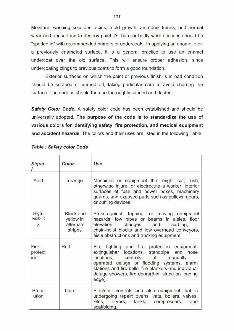
Moisture, washing solutions, acids, mold growth, ammonia fumes, and normal
wear and abuse tend to destroy paint. All bare or badly worn sections should be
"spotted in" with recommended primers or undercoats. In applying an enamel over
a previously enameled surface, it is a general practice to use an enamel
undercoat over the old surface. This will ensure proper adhesion, since
undercoating clings to previous coats to form a good foundation.
Exterior surfaces on which the paint or previous finish is in bad condition
should be scraped or burned off, taking particular care to avoid charring the
surface. The surface should then be thoroughly sanded and dusted.
Saf e ty Colo r C o d e. A safety color code has been established and should be
universally adopted. The purpose of the code is to standardize the use of
various colors for identifying safety, fire protection, and medical equipment
and accident hazards. The colors and their uses are listed in the following Table.
Table : Safety color Code
Signal
Color Use
Alert orange Machines or equipment that might cut, rush, otherwise injure, or electrocute a worker: interior surfaces of fuse and power boxes, machinery guards, and exposed parts such as pulleys, gears, or cutting devices.
High-visibilit
y
Black and yellow in alternate stripes
Strike-against, tripping, or moving equipment hazards: low pipes or beams in aisles, floor elevation changes and curbing, chain-hoist blocks and low overhead conveyors, aisle obstructions and trucking equipment.
Fire-protection
Red Fire fighting and fire protection equipment: extinguisher locations, standpipe and hose locations, controls of manually operated deluge or flooding systems, alarm stations and fire bells, fire blankets and individual deluge showers, fire doors(8-in. stripe on leading edge).
Precaution
blue Electrical controls and also equipment that is undergoing repair: ovens, vats, boilers, valves, kilns, dryers, tanks, compressors, and scaffolding.
131
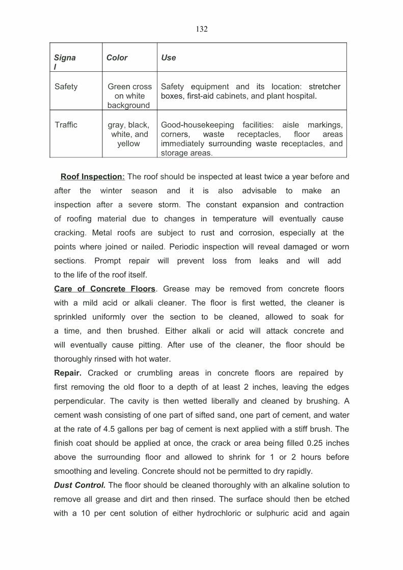
Signal
Color Use
Safety Green cross on white
background
Safety equipment and its location: stretcher boxes, first-aid cabinets, and plant hospital.
Traffic gray, black, white, and
yellow
Good-housekeeping facilities: aisle markings, corners, waste receptacles, floor areas immediately surrounding waste receptacles, and storage areas.
Roof Inspection : The roof should be inspected at least twice a year before and
after the winter season and it is also advisable to make an
inspection after a severe storm. The constant expansion and contraction
of roofing material due to changes in temperature will eventually cause
cracking. Metal roofs are subject to rust and corrosion, especially at the
points where joined or nailed. Periodic inspection will reveal damaged or worn
sections. Prompt repair will prevent loss from leaks and will add
to the life of the roof itself.
Care of Concrete Floors. Grease may be removed from concrete floors
with a mild acid or alkali cleaner. The floor is first wetted, the cleaner is
sprinkled uniformly over the section to be cleaned, allowed to soak for
a time, and then brushed. Either alkali or acid will attack concrete and
will eventually cause pitting. After use of the cleaner, the floor should be
thoroughly rinsed with hot water.
Repair. Cracked or crumbling areas in concrete floors are repaired by
first removing the old floor to a depth of at least 2 inches, leaving the edges
perpendicular. The cavity is then wetted liberally and cleaned by brushing. A
cement wash consisting of one part of sifted sand, one part of cement, and water
at the rate of 4.5 gallons per bag of cement is next applied with a stiff brush. The
finish coat should be applied at once, the crack or area being filled 0.25 inches
above the surrounding floor and allowed to shrink for 1 or 2 hours before
smoothing and leveling. Concrete should not be permitted to dry rapidly.
Dust Control. The floor should be cleaned thoroughly with an alkaline solution to
remove all grease and dirt and then rinsed. The surface should then be etched
with a 10 per cent solution of either hydrochloric or sulphuric acid and again
132

rinsed. Finally, a floor-hardening compound such as a dilute solution of sodium
silicate should be applied.
133