Instructions for use

Title A Theoretical Study on Multiscale Reaction Network Extracted from Single Molecule Time Series

Author(s) SULTANA, Tahmina

Issue Date 2014-03-25

DOI 10.14943/doctoral.k11402

Doc URL http://hdl.handle.net/2115/55711

Type theses (doctoral)

File Information Tahmina_Sultana.pdf

Hokkaido University Collection of Scholarly and Academic Papers : HUSCAP

A Theoretical Study on MultiscaleReaction Network Extracted from

Single Molecule Time Series

Tahmina Sultana

A thesis submitted for the degree of

Doctor of Philosophy (PhD)

2014

1. Reviewer: Prof. Tamiki Komatsuzaki

2. Reviewer: Prof. Makoto Demura

3 Reviewer: Prof. Masataka Kinjyo

4. Reviewer: Prof. Akimasa Fukui

5. Reviewer: Prof. Hiroshi Teramoto

6. Reviewer: Prof. Chun-Biu Li

Day of the defense:

Signature from head of PhD committee:

ii

Abstract

Ensemble experiments can access only average characteristics of biomolecular systems, thus, the

individual behavior of single molecules cannot be distinguished. In contrast, single molecule (SM)

experiments manifest the detailed complexity in kinetics and dynamics of these multiscale biological

processes at the single molecule level. The complex dynamics of single molecules, such as the On/Off

blinking of nano-particles, the opened/closed gating of ion channels, the bound/unbound kinetics in cell

signaling processes, are often probed experimentally in the form of time series with finite discrete levels.

The main goal of SM experiments is to extract kinetics and dynamical information from the observable

time series. However, how one can extract such information from an observed one-dimensional time

series is still an unresolved question.

In the analysis of SM time series, hidden Markov models (HMM) are often used to provide insights

on the complex mechanism of molecular machinery. To derive HMM from SM time series that incor-

porates non-exponential kinetics and molecular memory is one of the most contemporary and intriguing

subjects in the analysis of single molecule biology. In this thesis, I reviewed a recently developed math-

ematical approach which provides not only interpretation of the complex kinetics but also new insights

into biological function buried in ensemble measurements. This method, based on information theory,

is free from any a priori assumption, such as local equilibrium, detailed balance, or number of states.

Mathematically, it is proved that its scheme is the simplest representation that can predict the future

outcome maximally. This approach is known as State Space Network (SSN). The SSN is a type of

HMM that takes into account both multiple states buried in the measurement and memory effects in the

process of the observable whenever they exist. The states of SSN depend not only on the present value

of the observable but also on the past values along the course of time evolution so that the state-to-state

transitions are Markovian even though dynamical correlation may exist in the time series.

The scheme of SSN was based on the assumption that a given time series is stationary and long

enough. Time series obtained from SM experiments always suffer from as an insufficient number of

data points and sometimes may be non-stationary. To overcome these difficulties, a generalization of

SSN was developed by using a multiscale decomposition scheme based on discrete wavelet transforms

in our laboratory (1). The main drawback to apply this decomposition scheme to time series is that

it depends on the choice of wavelet basis function. Instead of wavelet decomposition, I introduced a

simple but efficient skipping step method (SSM) to decompose the original time series into a set of time

series at different timescales. The SSM can deal with the nature of multiscale nature and nonstationarity

for a discrete time series in the framework of SSN.

Previously, in an in vitro reconstituted system of the recognition process between epidermal growth

factor receptor (EGFR) on the plasma membrane and its adaptor protein Ash/Grb2 (2), non-exponential

iv

kinetics in the association and dissociation processes were found. In addition, the association kinetics

abnormally depends on the concentration of Grb2 owing to reaction memory concealed in the confor-

mation of EGFR. Two extreme reaction schemes for the association process were proposed (3); one of

them is called defect diffusion model in which, the system visits many dissociated states with different

rate constants to reach a specific target state for association. The other is called multiple-reaction chan-

nel model where all (dissociated) states with different association rate constants directly connected to

the associated state independently. However, they could not identify the actual, most plausible kinetic

scheme that reflects the observed kinetics objectively.

To demonstrate the versatility of my scheme, I investigated the time series of the EGFR-Grb2 sys-

tem. It was found that a newly-derived analytical expression of autocorrelation function from SSN

combined with SSM successfully reproduce the autocorrelation for a wide range of timescale up to the

timescale that loses the memory, 3 s. It was found that the underlying SSNs are in between the de-

fect diffusion model and multiple-reaction channel model and change their topographical structure as a

function of the timescale: while the corresponding SSN is simple at the short timescale (0.033 s to 0.1

s), the SSN at the longer timescales (0.1 s to 3 s) becomes rather complex in order to capture multiscale

kinetics emerging at longer timescales.

The Y1068F mutant of EGFR replaced tyrosine (Y) 1068 in EGFR (whose phosphorylation has been

reported to construct the primary strong Grb2 binding site) for analyzing the exponential properties and

memory effects in association and dissociation kinetics. The SSNs for the mutant (Y1068F) EGFR

are simpler than the wild type EGFR, indicating the existence of non-Markovian nature in the wild

type more than the mutant (Y1068F) EGFR. In addition, the SSN can capture the heterogeneity of the

memory in the process depending on each state. By looking into splitting patterns as an increase of

the history length for the shortest time scale SSN of the wild type EGFR at low concentration of Grb2,

it was found that visiting the unbound form of the wild EGFR-Grb2 system approximately resets all

information of history or memory of the process.

To implement the direct relationship between the states in the multiscale SSNs and the underlying

high-dimensional conformation of the system, it is necessary to construct a series of SSNs in terms of a

set of different single-molecule time series data from systematic mutations of amino-residues. I expect

that one may identify which amino residues perform to yield non-Markovian kinetics by monitoring the

morphological changes of the network. This may be regarded as ϕ value analysis of protein folding

kinetics to infer the energy landscape in the framework of SM biology.

v

vi

To my son Aydin Arushanyan Zaman

Acknowledgements

There are many people who have related to my life throughout this four and half years in

Japan. First and foremost I would like to thank my advisor, Prof. Tamiki Komatsuzaki. He

has been a phenomenal mentor, provided inspiration, kept me motivated and taught me in

countless ways with allowing me personal and intellectual freedom. I was surprised when

I found that he was working for me even in holidays. His personalities impressed me so

much that I want to be a teacher like him in the near future.

I wish to express my deep gratitude to Prof. Chun-Biu Li for his invaluable guidance, con-

stant encouragement, priceless suggestions, supports and share his rich experiences during

the progress meeting in our group. He always dealt with me as an independent researcher.

It was difficult to understand him at beginning, but somehow he has taught me in a right

way so that I could improve myself. His comments, suggestions, and advices will be with

me forever.

I am truly thankful to Dr. Hiroshi Teramoto for his direct and indirect help during my work.

He is the kindest person in the world I ever met. All students in our group love him so much

his friendly behavior and kindness. I have many happy memories with him.

I would like to thank my experimental collaborators Dr. Hiroaki Takagi in Department

of Physics, Nara Medical University, Dr. Miki Morimatsu in WPI Immunology Frontier

Research Center (WPI-IFReC),Osaka university, and Chief director, Dr. Yasushi Sako in

Cellular Informatics Laboratory, RIKEN. Without them my work could not be fulfilled.

Dr. Taylor, Dr. Nishimura and Dr. Kawai in our group have helped me to understand my

research deeply. Their comments about my research improved my study.

I am very glad that I had a chance to meet friends in my laboratory, especially I want to

mention the following names Sei, Itoh, Baba, Asfaw, Liu, Miyagawa, Nagahata, Chiba,

Kikuchi, Nag, Ibe, Niikura, Tsuda and Wang. They gave me a joyful life in Japan.

I like to thank our previous and present secretaries Ms. Kayo Abe and Ms. Maiko Mu-

ramoto for their kind supports in my student life in Japan.

Last but not the least, my family and the one above all of us, the omnipresent God (Al-

lah), for answering my prayers for giving me the strength to plod on despite my feeling of

resignation I sometimes got, which would make me give up and throw in the towel.

Thank you so much Dear Allah.

iv

Contents

List of Figures vii

List of Tables xi

1 Introduction 1

2 Theory 9

2.0.1 A brief description of how to construct State Space Network (SSN) . . . . . . 9

2.0.1.1 The Deterministic Properties of the Constructed SSN . . . . . . . . 12

2.0.2 Derivation of Time Autocorrelation Function . . . . . . . . . . . . . . . . . . 13

2.0.3 Expression for Dwell Time Distribution: . . . . . . . . . . . . . . . . . . . . . 16

2.0.4 Skipping Step Method (SSM) . . . . . . . . . . . . . . . . . . . . . . . . . . 18

3 Result and Discussion 23

3.1 An Illustration of our Construction Scheme of Multiscale SSNs for a Three-State Marko-

vian Network . . . . . . . . . . . . . . . . . . . . . . . . . . . . . . . . . . . . . . . 23

3.1.1 Application to Recognition Kinetics between EGFR and Grb2 . . . . . . . . . 28

3.1.1.1 A Brief Description of an in vitro Reconstituted Receptor-Adapter

Recognition Experiment . . . . . . . . . . . . . . . . . . . . . . . . 28

3.1.2 Correlations in Recognition Kinetics and the Underlying SSNs . . . . . . . . . 29

3.1.3 Heterogeneity of Non-Markovian Property Buried in SSNs . . . . . . . . . . . 35

3.2 Meassure to quantify the possibility of Dwell time distribution . . . . . . . . . . . . . 36

4 Conclusion 41

4.1 Conclusion and Perspectives . . . . . . . . . . . . . . . . . . . . . . . . . . . . . . . 41

v

CONTENTS

5 Appendix 45

5.0.1 Overview of EGFR and EGFR family . . . . . . . . . . . . . . . . . . . . . . 45

5.0.2 Grb2 . . . . . . . . . . . . . . . . . . . . . . . . . . . . . . . . . . . . . . . 47

5.1 Persistence of Markovian state with different skipping times . . . . . . . . . . . . . . 47

5.1.1 Result of Lpast and significance Level . . . . . . . . . . . . . . . . . . . . . . 50

5.1.2 Results of autocorrelation of the wild type and the Y1068F mutant at 10 and

100 nM Grb2 . . . . . . . . . . . . . . . . . . . . . . . . . . . . . . . . . . . 52

5.1.3 The Visualization of the underlying SSNs of the wild type and the Y1068F

mutant at 10 and 100 nM Grb2 and their lifetime constants . . . . . . . . . . . 56

References 57

vi

List of Figures

1.1 Dissociation kinetics: Cumulative histograms of the OFF dwell times for each concentration of

Grb2 were fitted with a single (green) and a sum of two (blue) or three (red) exponential functions.

Time constants are from fitting with the three exponential functions. Numbers in the parentheses

are percentages of each fraction. The time constants (for major component) were not inversely

proportional to the Grb2 concentration. This figure was published from (2). . . . . . . . . . . 4

1.2 The brief procedure to extract the underlying multiscale SSNs from the observed fluorescence

intensity time series of EGFR and Grb2 association process. (a) a schematic picture of the in

vitro reconstituted system of signal processing in a single cell. The time duration of the bind-

ing between EGFR and Grb2 can be monitored from the duration of high fluorescence intensity

from Cy3 attached to Grb2 detected using total internal reflection fluorescence microscope. In

the in vitro experiment, repeated binding and release of fluorescent spots at the same position

on the glass surface were observed up to a sufficiently long period (18 min). These correspond

to the interaction between Cy3- Grb2 and phosphorylated EGFR in the plasma membrane frag-

ments attached to the glass coverslip. Because simultaneous binding or release of multiple spots

at the same position on the glass surface were hardly detected, EGFR is considered to exist in

the monomer form (2). (b) the fluorescence intensity time trace reflecting the bound (ON) and

unbound (OFF) forms of Grb2 to EGFR. In the data analysis, the time series were transformed

into binary time series, from which the SSNs are constructed. (c) autocorrelation function and

the associated SSNs for different timescales. The solid line and different color dots denote the

autocorrelation obtained from the discrete time series, and the analytical evaluation based on the

SSNs, respectively. . . . . . . . . . . . . . . . . . . . . . . . . . . . . . . . . . . . . . 6

vii

LIST OF FIGURES

2.1 An illustrative example of the SSN construction procedure as a function of Lpast by using a binary

time series . . .UBUUBBUBUBB . . . where B and U denote, e.g., two distinct conformations. (a)

Lpast = 0. (b) Lpast = 1. (c) Lpast = 2. (d) Lpast = 3. The state is represented by a circle. The

directed links between the states is represented by a label with the next symbol to be generated by

the transitions and the corresponding transition probabilities inside the parenthesis for the link. . 11

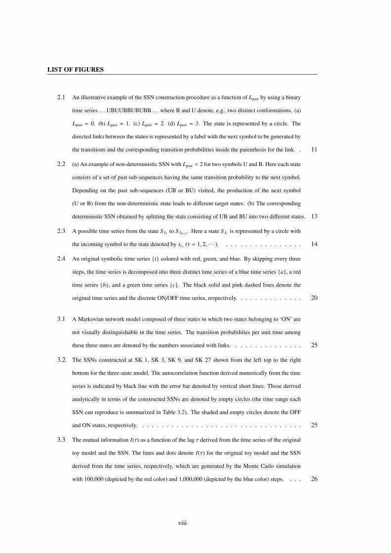
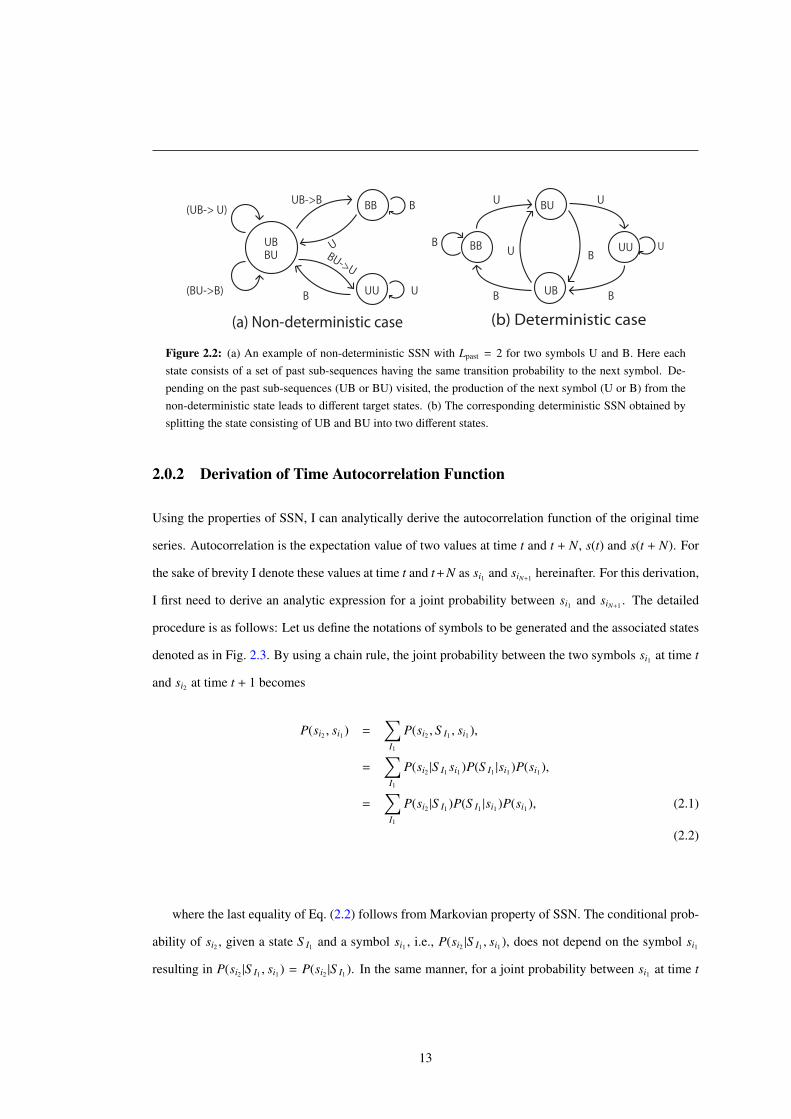
2.2 (a) An example of non-deterministic SSN with Lpast = 2 for two symbols U and B. Here each state

consists of a set of past sub-sequences having the same transition probability to the next symbol.

Depending on the past sub-sequences (UB or BU) visited, the production of the next symbol

(U or B) from the non-deterministic state leads to different target states. (b) The corresponding

deterministic SSN obtained by splitting the state consisting of UB and BU into two different states. 13

2.3 A possible time series from the state S I1 to S IN+1 . Here a state S Iτ is represented by a circle with

the incoming symbol to the state denoted by siτ (τ = 1, 2, · · · ). . . . . . . . . . . . . . . . . 14

2.4 An original symbolic time series {i} colored with red, green, and blue. By skipping every three

steps, the time series is decomposed into three distinct time series of a blue time series {a}, a red

time series {b}, and a green time series {c}. The black solid and pink dashed lines denote the

original time series and the discrete ON/OFF time series, respectively. . . . . . . . . . . . . . 20

3.1 A Markovian network model composed of three states in which two states belonging to ‘ON’ are

not visually distinguishable in the time series. The transition probabilities per unit time among

these three states are denoted by the numbers associated with links. . . . . . . . . . . . . . . 25

3.2 The SSNs constructed at SK 1, SK 3, SK 9, and SK 27 shown from the left top to the right

bottom for the three-state model. The autocorrelation function derived numerically from the time

series is indicated by black line with the error bar denoted by vertical short lines. Those derived

analytically in terms of the constructed SSNs are denoted by empty circles (the time range each

SSN can reproduce is summarized in Table 3.2). The shaded and empty circles denote the OFF

and ON states, respectively. . . . . . . . . . . . . . . . . . . . . . . . . . . . . . . . . . 25

3.3 The mutual information I(τ) as a function of the lag τ derived from the time series of the original

toy model and the SSN. The lines and dots denote I(τ) for the original toy model and the SSN

derived from the time series, respectively, which are generated by the Monte Carlo simulation

with 100,000 (depicted by the red color) and 1,000,000 (depicted by the blue color) steps. . . . 26

viii

LIST OF FIGURES

3.4 The third-order correlation functions C(τ1, τ2) as a function of τ1 with some fixed values of τ2,

derived numerically from the time series generated by the original model (indicated by the solid

lines) and that by the SSN (dots). Different colors mean the different values of τ2, i.e., τ2 = 0

(red), 2 (green), 4 (light blue), 6 (black), 8 (dark blue), and 10 (purple). The total Monte Carlo

step is 100,000. . . . . . . . . . . . . . . . . . . . . . . . . . . . . . . . . . . . . . . . 27

3.5 A schematic picture of the in vitro reconstituted system of signal processing. The time duration

of the binding between EGFR and Grb2 can be monitored from the duration of high fluorescence

intensity from Cy3 attached to Grb2 detected using total internal reflection fluorescence micro-

scope. These correspond to the interaction between Cy3-Grb2 and phosphorylated EGFR in the

plasma membrane fragments attached to the glass coverslip. . . . . . . . . . . . . . . . . . . 29

3.6 Autocorrelation for the ON/OFF time series of the association and dissociation processes between

the wild type and the Y1068F mutant at 1nM concetnration of Grb2. The autocorrelation function

derived numerically from the time series is indicated by black line in the wild type and gray line in

the mutant with the error bar denoted by vertical short lines. Those derived analytically in terms

of the constructed SSNs are denoted by open circles. . . . . . . . . . . . . . . . . . . . . . 31

3.7 The SSNs of the wild type and the Y1068F mutant at 1 nM concentration of Grb2 for different

skipping steps. The horizontal axis reflects the mutual proximity of the transition probability dis-

tributions associated with the individual states in arbitrary unit (a.u.) (See the text in detail). The

choice of vertical axis is arbitrary. Open (gray colored) circles denote the ON (OFF) states. The

states enclosed by the dashed curve in SK 9 for mutant emphasize that their transition probabili-

ties are almost identical. The size of the circle is proportional to the logarithm of the residential

probability of the state: the bigger the circle is, the longer the system resides in that particular state

(for visualization of the states whose area is less than 0.005 a.u.2, I introduced the minimum size

of 0.005 a.u.2). The red (black) colored links assign as producing next symbol ‘0’ (‘1’) (whose

destination is either of the OFF (ON) states). The weight of the links reflects the state-to-state

transition probabilities. . . . . . . . . . . . . . . . . . . . . . . . . . . . . . . . . . . . 33

3.8 The state splitting as increasing Lpast at 1 nM for the recognition reaction between the wild type

and the Y1068F mutant EGFR, and Grb2. (a) Lpast=1, (b) Lpast=2, (c) Lpast=3, (d) Lpast=4 and (e)

Lpast=5. The meaning of state, links and their colors are the same as in Fig. 3.7. . . . . . . . . 40

ix

LIST OF FIGURES

5.1 Basic Structure of EGFR demonstrating relevant domains. (I) The extracellular region consists

of four domains ( two of them are rich in cysteine). (II) Transmembrane domains. (III) The in-

tracellular domains:(1) juxtamembrane domain; (2) tyrosine kinase domain; (3) regulatory region

domain. The phosphorylation of several substrates by the tyrosine kinase domain of the EGFR

receptor is responsible for activating the various signaling cascades that are shown in the tail of

the EGFR in the cytosol. This figure was published from Refs. (4, 5). . . . . . . . . . . . . . 46

5.2 Very simple schematic example of intracellular signaling pathway activated EGFR and receptor

tyrosine kinases. EGFRs dimerize in response to ligand binding. The ligand response is trig-

gered into tyrosine kinase at which docking protein Grb2, which contains a domain that binds to

the phosphotyrosine residues of the activated receptor. Then complex Grb2-SOS promotes the

removal of GDP from a member of the Ras subfamily. Ras can then bind GTP and become ac-

tive. After then activated Ras activates the protein kinase activity of RAF kinase. RAF kinase

phosphorylates and switch on MEK (MEK1 and MEK2). MEK phosphorylates and operates a

mitogen-activated protein kinase (MAPK) and finally activate nucleus or DNA (6). . . . . . . . 48

5.3 The statistical complexity versus Lpast for different significance levels α in the Kolmogorov-

Smirnov test for SK 1, with α = 0.1, 0.05, 0.01, 0.005 and 0.001 for both (a) the three states

model (Sec. 3.1) and the association and dissociation reaction between the wide type EGFR and

Grb2 at (b) 1 nM, (c) 10 nM, and (d) 100 nM. Different colors correspond to different values of α:

red 0.1, green 0.05, pink 0.01, black 0.005, and blue 0.001. In (a) Lpast = 2 results in a converged

SSN for the three states model. In the wild type EGFR case, Lpast = 3 was chosen to yield the

approximate (local) convergent network for (b) 1 nM, (c) 10 nM and (d) 100 nM. . . . . . . . 51

5.4 Autocorrelation for the ON/OFF time series of the association and dissociation processes between

the wild type and the Y1068F mutant at 10 nM concentration of Grb2. See the caption of Fig. 3.6. 52

5.5 Autocorrelation for the ON/OFF time series of the association and dissociation processes between

the wild type and the Y1068F mutant at 100 nM concentration of Grb2. See the caption of Fig. 3.6. 53

5.6 The SSNs of the wild type (right) and the Y1068F mutant (left) at 10 nM concentration of Grb2

for different skipping steps (SK 1, 3, 9, and 27 from the top to the bottom). See also the caption

of Fig. 5.6 in the main text. . . . . . . . . . . . . . . . . . . . . . . . . . . . . . . . . . 54

5.7 The SSNs of the wild type (right) and the Y1068F mutant (left) at 100 nM concentration of Grb2

for different skipping steps (SK 1, 3, 9, and 27 from the top to the bottom). See also the caption

of Fig. 5.6. . . . . . . . . . . . . . . . . . . . . . . . . . . . . . . . . . . . . . . . . . 55

x

List of Tables

3.1 The residential probabilities of the three-state model and the corresponding SSN. The SSN is

constructed with the significance level α = 0.01, Lpast = 2 and the skipping step one. The state S 0

contains subsequences 11, the state S 1 01, and the state S 2 10 and 00, respectively. . . . . . . . 24

3.2 The time region for which each SSN constructed for different skipping step 1, 3, 9, and 27 re-

produces the autocorrelation. Note that the increment of the intervals is different with each other

dependent on the SK m, and the total step length is 100,000. . . . . . . . . . . . . . . . . . . 24

3.3 The time intervals for which the autocorrelation is reproduced by each SSN constructed for each

different skipping step at three different concentration of Grb2 for the wild type EGFR. Note again

that the increment of the time intervals is different with each other dependent on the SK m: 0.033

s, 0.1 s, 0.3 s, and 0.9 s for m =1, 3, 9, and 27, respectively. The unit of time is in second. . . . 34

3.4 The time intervals for which the autocorrelation is reproduced by each SSN constructed for each

different skipping step at three different concentration of Grb2 in the case of the Y1068F mutant

EGFR. See also the caption in Table 3.3. . . . . . . . . . . . . . . . . . . . . . . . . . . . 34

5.1 The lifetime constants of the wild type EGFR at all concentration of Grb2 for each state space

network. The lifetime constants are calculated from Eq. (5) (in the main text) and their weights

are shown in parentheses. . . . . . . . . . . . . . . . . . . . . . . . . . . . . . . . . . . 56

5.2 The lifetime constants of the Y1068F mutant EGFR at all concentration for each state space

network (The unit is of second). See also the caption of Table 5.1. . . . . . . . . . . . . . . . 56

xi

LIST OF TABLES

xii

1

Introduction

Protein-protein interactions play a vital role in biomolecular system of living cells, such as cell signaling

in a cell which is comprised of a series of protein molecules and their interactivities. These protein

interactions often involve in complex mechanisms and that show inhomogeneous dynamics, because of

the significant conformational changes in proteins. Moreover, the dynamics may be different from time

to time for the same individual molecules (7, 8, 9, 10, 11, 12, 13, 14, 15). These protein interactions

even at single molecule level are amplified along the signaling pathways. So it is crucially important to

study the underlying mechanism of protein interaction at both ensemble and single levels to extract the

root of protein interactions in the cell signaling.

There are several well known techniques such as gel filtration, Western blotting, nuclear magnetic

resonance (NMR), X-ray crystallography etc, by which one can get information about proteins and their

reactions. In gel filteration method one obtained information about macroscopic level of protein such

as the molecular weight distribution etc. NMR and X-ray crystallography are used to investigate highly

dynamic, partial inhomogeneous molecules and complexes. Recently NMR static and ensemble struc-

tural studies of protein complexes indicate that protein interaction sites or domains undergo dramatic

conformational changes from disordered to ordered states upon complex formation (16). However, in-

homogeneity and complexity of protein conformational (structural) changes are extremely difficult to

be identified and analyzed in an ensemble measurement e.g., NMR, X-ray clystrallography etc, because

they can access only averaged characteristics, thus the individual behavior of single molecules cannot

be characterized. Therefore, to characterize inhomogeneous, static and dynamic disorder (13, 14, 17),

memory landscapes (18) of enzymatic reactions, as well as dynamic polymorphisms of protein struc-

tures (19, 20), single-molecule (SM) experiments are useful because they remove the inhomogeneity

and manifest the detailed complexity in dynamics of these multiscale protein-protein process by study-

1

1. INTRODUCTION

ing one molecule at a time (2, 21). SM experiments have allowed researchers to explore small scale

systems with high spatial and temporal resolution. Main advantage of this type of experiment is the re-

moval of ensemble averaging by creating the actual distribution of values for an experimental observed

parameter (e.g. wavelength, intensity etc) (2). It is able to reveal and diagnose the events of extremely

low probability i.e., repeatedly excitation of one molecule or measuring hundreds of different molecules

and identify previously unknown reaction intermediates (22).

The complex dynamics of a single-molecule systems, such as the ON/OFF blinking of nano-particles

(23), the opened/closed gating of ion channels (24, 25), the bound/unbound kinetics (2) in cell signaling

processes, are often probed experimentally in the form of time series with finite discrete levels, and such

time traces contain detailed dynamic information. The main goal of SM measurement is to extract the

kinetics and dynamical information from such direct observable time trace (2, 15, 18, 21, 22, 23, 26, 27,

28, 29, 30, 31, 32). It obviously comes to mind that, what information and how can one learn from such

one dimensional time series? How to identify the pattern buried in SM time series? How many states

exist on this time series? How are they connected?. Those are very regular questions for analyzing time

series. So, it is necessary to establish a firm theoretical modeling method of the underlying mechanism

of molecular machinery from observed SM time series to explore single molecule dynamics. From

this perspective, it is useful to introduce a computational, data- or hypothesis- driven approaches in an

effort to facilitate the discovery of the kinetics in the process. There are many conventional data-driven

techniques in terms of interpreting and analyzing SM measurements, such as multi-parametric networks

based on Monte Carlo simulation (33), reaction diffusion model with photon statistics (34), hidden

Markov model (1, 35, 36, 37, 38, 39, 40, 41, 42, 43, 44, 45), aggregated markov model (46, 47, 48), semi-

Markovian kinetic scheme (49), kinetic network model (50), and also Bayesian approach (51). Markov

process is very commonly used to interpret kinetics because of its useful and convenient properties even

though the observable data may not be a Markov chain.

In the analyses of SM time series, Hidden Markov Model (HHM) are often used to provide insights

on the complex mechanism of molecular machinery (1, 35, 36, 37, 38, 39, 40, 41, 42, 43, 44, 45).

However, to derive HMM from single molecule time series that incorporates non-exponential behavior

and molecular memory of the process and, to assign the physical correspondence of the constructed

states are yet one of the most contemporary and intriguing subjects to be resolved. Moreover, most

existing methods (for mathematical modeling) depend on a huge amount of fitting parameters, e.g.,

algorithms using maximum likelihood estimator to obtain the parameters of the HMM (22). These

methods, in general, require the initial assumption of model parameters, such as network structure and

number of states.

2

Recently a novel data-driven modeling was developed to naturally derive the underlying multiscale

state space network (SSN) from single molecule time series based on information theory (1, 39, 40, 52,

53, 54). The SSN is regarded as a certain type of HMM that represents the complex kinetics such as non-

exponentiality and the molecular memory of the process, and identifies the physical correspondence.

The states of SSN depend not only on the present value of the observable but also on the past information

along the course of time evolution so that the state-to-state transitions are Markovian even dynamical

correlation may exist in the time series. In addition, most conventional methods (e.g. HMM) are state-

labeled i.e., producing a symbol when a state is visited. On the other hand, the SSN is edge-labeled

i.e., producing a symbol when a transition is made. I newly derive an analytic expressions of kinetic

properties such as autocorrelation function and dwell time distribution of a given discrete time series in

terms of the intrinsic properties of SSNs.

The original idea of the SSN was developed in 1980s (52, 53, 54) aiming at discovering the pattern

or module of dynamical features buried in a given stationary time series. Time series obtained from

SM experiments always suffer from the problem of insufficient number of data points and sometimes

may be non-stationary. To overcome these difficulties, a generalization of SSN has been developed

in our laboratory by using a multiscale decomposition scheme based on discrete wavelet transforms to

decompose the time series into components at different scales (1, 39, 40). It has been reported (1, 39, 40)

in a single-molecule electron transfer experiment of the NADH: flavin oxidoreductase(Fre) complex (55)

that the topographical features of the SSN change as a function of timescales to capture the transition

from abnormal to normal diffusion observed in the protein fluctuation. The main drawback to apply

this decomposition scheme to the time series is that it depends on the choice of wavelet basis function.

Instead of wavelet decomposition, here I introduced a simple, but efficient skipping step method (SSM)

to decompose the original time series into a set of time series at different timescales. The SSM can deal

with the nature of multiscale and nonstationarity for a discrete time series in the framework of SSN.

To demonstrate my methods, I analyzed the time series measured in an in vitro reconstituted system

(by Morimatsu et al.) of the recognition process between epidermal growth factor receptor (EGFR)

on the plasma membrane and its adaptor protein Ash/Grb2 (2). EGFR is a single membrane spanning

protein, which associates with EGF at the extracellular matrix of the cell, the association between them

induces conformational changes in the extracellular domain of EGFR that transmit the external signal

into the cytoplasm. Thus Grb2 (is one of the adapter protein of EGFR) links activated EGFR to down-

stream signaling molecules to induce functional changes in cells (See Appendix for more detail) (2).

To understand the signal flows in the cells comprehensibly, it is important to clarify the association and

dissociation kinetics between EGFR and whole molecules of Grb2, as it is the initial key stage inside the

3

1. INTRODUCTION

cell. Previously, it has been studied only dissociation process of this system using surface plasmon res-

onance (56, 57) and tryptophan fluorescence (58). Morimatsu et al.(2) first time studied the association

and dissociation kinetics between EGFR and Grb2 at the single molecule level. In the SM experiments

(2), they observed the repeated binding and release of fluorophore Grb2-Cy3 at different concentra-

tion of Grb2. They measured the durations from the onset of association to the dissociation of Grb2

molecules and from the dissociation of Grb2 molecule to the association of the next Grb2 molecule.

Dissociation and association kinetics between EGFR and Grb2 were analyzed by the distribution of

ON dwell times(=waiting time for dissociation) and OFF dwell times(=waiting time for association).

It was found that dissociation and association process between EGFR and Grb2 showed non-single ex-

ponential kinetics, and the association kinetics depend nonlinearly on the concentration of Grb2. This

non-single exponential properties and concentration dependency of Grb2 were suggesting the existence

of molecular memory in the signaling process (2) (See Fig. 1.1).

Figure 1.1: Dissociation kinetics: Cumulative histograms of the OFF dwell times for each concentration ofGrb2 were fitted with a single (green) and a sum of two (blue) or three (red) exponential functions. Timeconstants are from fitting with the three exponential functions. Numbers in the parentheses are percentagesof each fraction. The time constants (for major component) were not inversely proportional to the Grb2concentration. This figure was published from (2).

4

For analyzing multiple-exponential kinetics in association process, two extreme reaction schemes

were proposed (3);

• Defect diffusion model: In this model, the system visits many unbounded (dissociated) states to

reach a specific target state for association, but the rate constants from one state to another state

are not unique. The main problem arises from this model is that only one special path exists for

the association that is not always possible in the real system. In addition, there is no path between

the associated state and the dissociated state.

• Multiple-reaction channels with different association rate constants: In this system, many un-

bound (dissociated) states exist and each of them are connected to associate state with different

association rate constants. Moreover, these dissociated states are independent from each other.

Likewise, there is no path from the associated state to the dissociated state.

However, they could not identify the actual, most plausible kinetic scheme that reflects the observed

kinetics objectively. Without any initial assumption of model parameters or more detailed information

about the correlation between reactions, one cannot reach a constructive conclusion from their investi-

gations.

In this thesis, I presented a data-driven HMM model (termed as SSN) with generalization to non-

stationary time series, which best balances all conflict arising in this system. In the SSN construction,

encoded past information in the state, SSNs are able to represent the complex kinetics such as non-

single exponential properties and molecular memories, and identify the physical correspondence of

EGFR-Grb2 process.

The objective of this research is to extract the most plausible kinetics properties of the recognition

between EGFR and Grb2 from one dimensional time series free from a priori assumption. This objective

will be completed by demonstrating two proposed schemes to EGFR-Grb2 process as well as describing

the association and dissociation kinetics between EGFR and Grb2 (2) from the properties of constructed

SSNs.

The overall outline of the thesis is schematically shown in Fig. 3.5: I extract SSNs at different

timescales that capture the association and dissociation process between EGFR and Grb2 from the ob-

served time series (2). It was found that the underlying SSNs are in between the defect diffusion model

and multiple-reaction channel model.

This thesis is organized as follows:

5

1. INTRODUCTION

ONOFF

Inte

nsi

ty

Time Step

(b)

Aut

ocor

rela

tion

(c)

Time(s)

P

P

P

P

P P

P

P

P

P P

P

P

P

P

EGF

EGFR

Plasma membrane

Grb2

Cy3association dissociation

OFF

(a)

0

0.2

0.4

0.6

0.8

1.0

1.2

0 10 20 30 40 50 60

intensity

symbolized intensity

ON

OFF

111

001

011

111

110

010001

101011

000

100

000

100

110

0.020

0.015

0.010

0.005

0.1 0.2 0.5 1.0 2.0 5.0

Figure 1.2: The brief procedure to extract the underlying multiscale SSNs from the observed fluorescenceintensity time series of EGFR and Grb2 association process. (a) a schematic picture of the in vitro reconstitutedsystem of signal processing in a single cell. The time duration of the binding between EGFR and Grb2 canbe monitored from the duration of high fluorescence intensity from Cy3 attached to Grb2 detected usingtotal internal reflection fluorescence microscope. In the in vitro experiment, repeated binding and releaseof fluorescent spots at the same position on the glass surface were observed up to a sufficiently long period(18 min). These correspond to the interaction between Cy3- Grb2 and phosphorylated EGFR in the plasmamembrane fragments attached to the glass coverslip. Because simultaneous binding or release of multiplespots at the same position on the glass surface were hardly detected, EGFR is considered to exist in themonomer form (2). (b) the fluorescence intensity time trace reflecting the bound (ON) and unbound (OFF)forms of Grb2 to EGFR. In the data analysis, the time series were transformed into binary time series, fromwhich the SSNs are constructed. (c) autocorrelation function and the associated SSNs for different timescales.The solid line and different color dots denote the autocorrelation obtained from the discrete time series, andthe analytical evaluation based on the SSNs, respectively.

6

• In Sec. 2: I briefly describe the construction procedure of the state space network (SSN) with its

one of the most important properties. Next I newly present an analytical expression of autocorre-

lation by using the general properties of the SSN. I also implement the dwell time distribution by

the previous manner. Owing to the lack of sample points and non-stationarity of the time series, I

introduce a simple scheme called skipping step method (SSM) to derive the underlying SSNs at

different timescales.

• In Sec. 3.1 : To illustrate my proposed methods, I applied both the theoretical methods to a

three-state Markovian network. It was found that, successfully constructed SSNs reproduce au-

tocorrelation function of three states Markovian network. The structure of SSNs of this model

changes as a function of number of time steps. When time step equals to nine, the SSN becomes

Markovian (which depends only on present time step) implying that, with more than nine steps

the system does not depend on the past. Finally I applied my SSN analysis combined with the

SSM to analyze fluorescence intensity time trace of the binding and unbinding processes between

EGFR and Grb2 under different concentrations of Grb2 in an in vitro reconstituted system (2).

The autocorrelation function from SSN combined with SSM successfully reproduce the autocor-

relation up to timescales that loses the memory. The SSNs change their topographical properties

as a function of timescale and the existence of multistate in this process and their connectivities

are newly established. In addition, the constructed SSN can capture the heterogeneity of the mem-

ory in the process depending on each state. By looking into splitting patterns as an increase of

the history length for the shortest time scale SSN of the wild type EGFR and the Y1068F mutant

of EGFR, I marked out the memory effects on association and dissociation kinetics (59) in this

thesis.

• In Sec. 4.1: In this section, I briefly describe the conclusion of my reseach including some

prospective futures works.

• In Appendix. 5.1: I reviewed some previous studies of EGFR and its family. Also I have showed

some important properties of the SSN and SSM.

7

1. INTRODUCTION

8

2

Theory

2.0.1 A brief description of how to construct State Space Network (SSN)

Here I present the brief procedure for constructing state space network (SSN) (53). If the underlying

kinetics have some memories (or information from the past events), the states in the SSN are defined

not only by the present value of the observable but also by the past subsequence(s) of the values (with a

specific range). In short, the range of the past subsequence denoted by Lpast hereinafter, corresponds to

the characteristic timescale of correlation of the event. This method starts from discretizing a continuous

time series x = {x(t1), x(t2) · · · , x(tN)} into a symbolic time series s = {s(t1), s(t2) · · · , s(tN)}. One does

not require the system in question to be locally equilibrated or satisfy detailed balance. The choice

of a suitable symbolization scheme and the number of symbols depend on the nature of time series,

experimental setup, signal-to-noise ratio, and so forth (40, 60, 61).

The second step is to evaluate the transition probabilities from different subsequences (called past

subsequences) to the future symbols, e.g., the transition probability P(si|s2s1) for any symbol si (i=1,...,

the total number of symbols) to appear at a time, say t, followed by a particular subsequence s2s1 in

which one observes a specific value s1 at time t − 1 and s2 at time t − 2 by tracing the whole time series.

Similarly, the transition probabilities for all other past subsequences s jsk with past length two will be

evaluated. The suitable value of Lpast depends on the nature of the underlying dynamics of the time

series: Lpast roughly corresponds to the characteristic timescale of correlation and Lpast is unity when

the process (the time series) is Markovian. The actual value of Lpast was taken to be the minimal value

at which the structural property of the constructed SSN does not change even when increasing the value

of Lpast (1) (See Appendix in detail).

The third step is to derive states in the network by using the transition probabilities for the past

subsequences. The transition probabilities for past subsequences whose length is optimal in capturing

9

2. THEORY

memory in the process provide all information required to predict the future. Then the question is this:

can I define a state by not the single instant value but the past subsequences along the time series?

Another feature to be desired for the kinetic scheme is to be simplest while maintaining the predictable

power. Therefore, states are defined as follows: for a given Lpast, if the transition probabilities are

regarded as the same, I group them together into a set called a “state” (denoted by S I hereinafter). This

is because all composite past subsequences in the “state” generate the same future symbols associated

with the same probabilities, implying that the grouping does not lose any predictable power while the

grouping simplifies and reduces the possible number of the states.

The final step is to link the states with each other to form a network. The transition probability

from a state S I to another state S J producing symbol s j, denoted by P(S J s j|S I), yields the weight of

the transition from S I to S J in the network with the generated s j. Here, the next state S J is uniquely

determined by the current state S I and the next symbol s j (see the next Sec. 2.0.1.1 for the special

case). Because all memory effects are encoded in the definition of states, the transition from S I to S J is

Markovian.

Now I demonstrate the above procedure by considering a simple binary time series . . .UBUUBBUBUBB . . .,

where B and U denote, for example, the bound and the unbound forms between a substrate and a re-

ceptor protein, respectively. Let us start to investigate the transition probability of zero length Lpast = 0.

This corresponds to the residential probability of each form U or B. Suppose that I have these values as

P(U|null) = 0.77 and P(B|null) = 0.23. Here the number of states is set to be one, and the prediction of

the future will be performed without any information of the current value of the time series and the past

subsequence (See Fig. 2.1(a)). Then I increase the value of Lpast by one and check if the network changes

by the increment in Lpast. Suppose again that I have P(U|U) = 0.91, P(B|U) = 0.09, P(U|B) = 0.33, and

P(B|B) = 0.67.

Since the transition probabilities from the given symbols U and B are different, I must have, at

least, more than two states (See Fig. 2.1(b) with Lpast = 1). If the transitions actually require only the

information of the current values, i.e., Markovian process in the time series, this SSN would be the

desired one. In order to confirm if this is the case, the process needs to continue by increasing Lpast

and check if the topological feature of the SSN does not change. For Lpast = 2, there are four possible

past subsequences {UU,UB,BB,BU} and imagine that their corresponding transition probabilities are

P(U|UU) = 0.90, P(B|UU) = 0.10, P(U|UB) = 0.21, P(B|UB) = 0.79, P(U|BU) = 0.90, P(B|BU) =

0.10, P(U|BB) = 0.39 and P(B|BB) = 0.61, respectively.

Since I group BU and UU but differentiate BB and UB as the individual states according to the rule

as in Fig. 2.1(c), the topology of the SSN changes from that with Lpast = 1. This implies that the SSN

10

BUB(0.23) U

B B

B U B

U U B

(0.77)U B

U U

B U

U B U U U

U B U

B B U

B U U

B B B

U B B

U(0.91)

B(0.09)

B(0.67)

U(0.33)

U(0.90)B(0.10)

U(0.21)

B(0.79)

B(0.61)

U(0.39)B(0.79)

B(0.61)

B(0.10)

U(0.21)

U(0.39)

U(0.90)

(a) (b)

(c) (d)

Figure 2.1: An illustrative example of the SSN construction procedure as a function of Lpast by using a binarytime series . . .UBUUBBUBUBB . . . where B and U denote, e.g., two distinct conformations. (a) Lpast = 0.(b) Lpast = 1. (c) Lpast = 2. (d) Lpast = 3. The state is represented by a circle. The directed links between thestates is represented by a label with the next symbol to be generated by the transitions and the correspondingtransition probabilities inside the parenthesis for the link.

11

2. THEORY

with Lpast = 1 is not the converged one and the process of the time series is not Markovian. Fig. 2.1(d)

shows the corresponding SSN with Lpast = 3. I find that the topographical features of the SSN is the

same as that with Lpast = 2. Therefore Lpast = 2 is regarded as the optimal Lpast yielding the converged

SSN. Once I refer to the one step forward in time from the current time for the prediction of the future

(Lpast = 2), the process of the “state”-to-“state” transitions becomes Markovian in nature although the

process of the “observable”-to-“observable”, i.e., time series of the observable itself, is non-Markovian

(Actually this binary time series in this example was generated from a three-states Markovian model

whose transition probabilities are taken from Fig.2.1(c)).

In practice, the convergence of the topographical nature of the SSN is thoroughly examined by

using the information amount (Shannon entropy for the residential probabilities of states in SSN) and

mathematically the converged SSN is regarded as the minimal but the most predictable model to capture

all the statistical information of a given time series. Readers who are interested in the mathematical

details can refer to the reviews (40, 53, 62).

2.0.1.1 The Deterministic Properties of the Constructed SSN

In the algorithm to construct the SSN from time series (62), the length of the future sequences, Lfuture,

is chosen to be one and only the length of the past subsequences, Lpast, is varied. The use of Lfuture = 1

aims to obtain a better statistical sampling of the transition probabilities, but on the other hand, the non-

deterministic situation can occur: a SSN is called deterministic if the current state with a next symbol

to be produced can uniquely identify the next state to be visited, otherwise called non-deterministic.

The advantage of the deterministic network is that there is a one-to-one correspondence between the

symbolic sequences (i.e., the time series) and the state sequences that are generated by the SSN. This

allows us to keep track of the time evolution of the states by referring to the time series.

Non-deterministic SSN can occur when Lpast > Lfuture. To guarantee the constructed SSN to be

deterministic, a simple procedure was employed in which non-deterministic states are made to split until

they become deterministic as illustrated in Fig. 2.2. In Fig. 2.2 (a), suppose that the state containing the

sequences UB and BU are combined together because their transition probabilities for future symbols

are regarded as the same. Nevertheless their target state to be visited is not uniquely fixed for a given

future symbol, e.g. the sequence BU links to the state containing the sequence UU by producing the

symbol U, whereas the sequence UB has a self-link to the same state by producing the same symbol U.

In this non-deterministic situation, we may not uniquely generate the corresponding state sequence from

the given time series. In such cases I split the sequences BU and UB from one state into two different

states to obtain the deterministic network as shown in Fig. 2.2(b).

12

UBBU

UU

BB

UU

BU

UB

BBB U

B

U B

U U

B

(UB-> U)

(BU->B)

UB->B

U

B

B

BU->U

U

(a) Non-deterministic case (b) Deterministic case

Figure 2.2: (a) An example of non-deterministic SSN with Lpast = 2 for two symbols U and B. Here eachstate consists of a set of past sub-sequences having the same transition probability to the next symbol. De-pending on the past sub-sequences (UB or BU) visited, the production of the next symbol (U or B) from thenon-deterministic state leads to different target states. (b) The corresponding deterministic SSN obtained bysplitting the state consisting of UB and BU into two different states.

2.0.2 Derivation of Time Autocorrelation Function

Using the properties of SSN, I can analytically derive the autocorrelation function of the original time

series. Autocorrelation is the expectation value of two values at time t and t + N, s(t) and s(t + N). For

the sake of brevity I denote these values at time t and t+N as si1 and siN+1 hereinafter. For this derivation,

I first need to derive an analytic expression for a joint probability between si1 and siN+1 . The detailed

procedure is as follows: Let us define the notations of symbols to be generated and the associated states

denoted as in Fig. 2.3. By using a chain rule, the joint probability between the two symbols si1 at time t

and si2 at time t + 1 becomes

P(si2 , si1 ) =∑

I1

P(si2 , S I1 , si1 ),

=∑

I1

P(si2 |S I1 si1 )P(S I1 |si1 )P(si1 ),

=∑

I1

P(si2 |S I1 )P(S I1 |si1 )P(si1 ), (2.1)

(2.2)

where the last equality of Eq. (2.2) follows from Markovian property of SSN. The conditional prob-

ability of si2 , given a state S I1 and a symbol si1 , i.e., P(si2 |S I1 , si1 ), does not depend on the symbol si1

resulting in P(si2 |S I1 , si1 ) = P(si2 |S I1 ). In the same manner, for a joint probability between si1 at time t

13

2. THEORY

0 1 1

1 2

12

-13

-1

Figure 2.3: A possible time series from the state S I1 to S IN+1 . Here a state S Iτ is represented by a circle withthe incoming symbol to the state denoted by siτ (τ = 1, 2, · · · ).

and si3 at time t + 2,

P(si3 , si1 ) =∑I2i2I1

P(si3 , S I2 , si2 , S I1 , si1 ),

=∑I2i2I1

P(si3 |S I2 )P(S I2 si2 |S I1 )P(S I1 |si1 )P(si1 ),

=∑I2i2I1

P(si3 |S I2 )T (i2)I2I1

P(S I1 |si1 )P(si1 ),

=∑I2I1

P(si3 |S I2 )(∑

i2

T (i2)I2I1

)P(S I1 |si1 )P(si1 ),

=∑I2I1

P(si3 |S I2 )TI2I1 P(S I1 |si1 )P(si1 ).

(2.3)

Here the transition probability P(S I2 si2 |S I1 ) is denoted by T (i2)I2I1

and, for the sake of simplicity, we

introduce a notation TI2I1 to represent TI2I1 =∑

i2 T (i2)I2I1

. To extend Eq. (2.3) for time t + 3 I get

P(si4 , si1 )

=∑

I3,i3,I2,i2,I1

P(si4 , S I3 , si3 , S I2 , si2 , S I1 , si1 ),

=∑

I3,i3,I2,i2,I1

P(si4 |S I3 )P(S I3 si3 |S I2 )P(S I2 si2 |S I1 )

P(S I1 |si1 )P(si1 ),

=∑

I3,i3,I2,i2,I1

P(si4 |S I3 )T (i3)I3I2

T (i2)I2I1

P(S I1 |si1 )P(si1 ),

=∑I3,I1

P(si4 |S I3 )

∑I2

TI3I2 TI2I1

P(S I1 |si1 )P(si1 ),

=∑I3I1

P(si4 |S I3 )(T2)I3I1 P(S I1 |si1 )P(si1 ).

(2.4)

14

Finally I get the expression for the joint probability between si1 at time t and siN+1 at time (t + N) as

follows:

P(siN+1 , si1 )

=∑

IN ,IN−1,··· ,I1

P(siN+1 |S IN )TIN IN−1 TIN−1IN−2 · · ·

TI3I2 TI2I1 P(S I1 |si1 )P(si1 ),

=∑IN I1

P(siN+1 |S IN )(TN−1)IN I1 P(S I1 |si1 )P(si1 ).

(2.5)

I factorize this transition matrix T into T = QΛQ−1 where Q means the square matrix (n × n) (n

is number of states in SSN) whose column is the eigenvector of the transition matrix, Λ the diagonal

matrix whose diagonal elements are the corresponding eigenvalues of the transition matrix, and Q−1 the

inverse matrix of Q, respectively. By using the factorization, Eq. (2.5) can be written as

P(siN+1 , si1 )

=∑IN I1

P(siN+1 |S IN )[(QΛQ−1)N−1

]IN I1

P(S I1 |si1 )P(si1 ),

=∑IN I1

P(siN+1 |S IN )(QΛN−1Q−1)IN I1

P(S I1 |si1 )P(si1 ),

=∑

C

∑IN

P(siN+1 |S IN )QINC

λN−1C∑

I1

Q−1CI1

P(S I1 |si1 )P(si1 )

,=∑

C

AC BCλN−1C ,N ≥ 1

(2.6)

where λC is the C-th diagonal element ofΛ and AC =∑

INP(siN+1 |S IN )QINC and BC =

∑I1

Q−1CI1

P(S I1 |si1 )P(si1 ).

Since T is a probability matrix, it always has one eigenvalue equal to unity.

The timescale(s) of correlation (called lifetime(s) tC) of the process can be calculated straightfor-

wardly by

tC = −1

log λC. (2.7)

15

2. THEORY

In the analysis of signal process, autocorrelation function is often used without normalization, that is,

without subtraction of the mean and division by the variance (63). Since my SSN behaves as a stationary

process at least for a timescale for which the SSN is constructed, I can define the autocorrelation function

as the expectation value of the two symbols s(t + τ) and s(t) without normalization, i.e.,

C(τ) = E[s(t + τ)s(t)]

=∑iτ+1i1

siτ+1 si1 P(siτ+1 , si1 )

=∑

C

∑iτ+1i1

siτ+1 si1 AC BCλτ−1C . (2.8)

2.0.3 Expression for Dwell Time Distribution:

Here I derive an analytical expression of dwell time distribution for a binary time series such as “· · · 111011100111000 · · · ”

where, for example, the symbol ‘1’ and ‘0’ correspond to ON and OFF level, respectively. Since I aim

to develop the probability distribution of PON(t) and POFF(t), I can write the ON level probability distri-

bution as:

PON(t) =P(0, 1, · · · , 1, 0)

P(0, 1, 0) + P(0, 1, 1, 0) + · · · + P(0, 1, · · · , 0),

=P(01t0)∑∞

t′=1 P(01t′0)

(2.9)

and∑∞

t=1 PON(t) = 1. Now I demonstrate it in terms of SSNs as follows: If the length of ON event is 1

P(0, 1, 0) =∑I1I2

P(0, S I2 , 1, S I1 , 0),

=∑I1I2

P(0|S I2 )P(S I2 1|S I1 )P(S I1 |0)P(0),

=∑I1I2

P(0|S I2 )T (1)I2I1

P(S I1 |0)P(0).

(2.10)

16

If the length of ON event is 2,

P(0, 1, 1, 0) =∑I1I2I3

P(0, S I3 , 1, S I2 , 1, S I1 , 0),

=∑I1I2I3

P(0|S I3 )P(S I3 1|S I2 )P(S I2 1|S I1 )

P(S I1 |0)P(0),

=∑I1I2I3

P(0|S I3 )T (1)I3I2

T (1)I2I1

P(S I1 |0)P(0),

=∑I1I3

P(0|S I3 )(T (1))2I3I1

P(S I1 |0)P(0).

(2.11)

So, if the length of ON event is t,

P(0, 1t, 0) =∑

I1···It+1

P(0|S It+1 )T (1)It+1It

T (1)It It−1· · ·

T (1)I2I1

P(S I1 |0)P(0),

=∑I1It+1

P(0|S It+1 )(T (1))tIt+1I1

P(S I1 |0)P(0).

(2.12)

Finally I can write the ON level probability as follows:

PON(t) =

∑I1It+1

P(0|S It+1 )(T (1))tIt+1I1

P(S I1 |0)P(0)∑∞t′=1 P(01t′0)

,

=

∑I1It+1

P(0|S It+1 )(T (1))tIt+1I1

P(S I1 |0)P(0)∑∞t′=1∑

I1It′+1P(0|S It′+1 )(T (1))t′

It′+1I1P(S I1 |0)P(0)

.

(2.13)

For more simplification the numerator can be written as following,∑I1It+1

P(0|S It+1 )(T (1))tIt+1I1

P(S I1 |0)P(0)

=∑I1It+1

P(0|S It+1 )(HΛ′H−1)tIt+1I1

P(S I1 |0)P(0),

=∑I1It+1

P(0|S It+1 )HIt+1c(λ′c)tH−1cI1

P(S I1 |0)P(0),

=∑

c

Lc(λ′c)tKc,

(2.14)

where Lc =∑

It+1P(0|S It+1 )HIt+1c and Kc =

∑I1

H−1cI1

P(S I1 |0)P(0).

17

2. THEORY

In above, I factorize the transition matrix T (1) into three matrices; H is the square matrix (n × n) (n

is number of states in SSN) whose column is the eigenvector of the transition matrix, Λ′ is the diagonal

matrix whose diagonal elements are the corresponding eigenvalues of the transition matrix, and H−1 is

the inverse matrix of H. I have T = HΛ′H−1 by diagonalization. For the denominator of Eq. 2.13, since

It′+1 and I1 are dummy variables, I can simply replace them by I′ and I respectively. The denominator

in Eq. 2.13 becomes

∞∑t=1

∑I′I

P(0|S I′ )(T (1))tI′I P(S I |0)P(0)

=

∞∑t=1

∑I′I

P(0|S I′ )(HΛ′H−1)tI′I P(S I |0)P(0),

=∑

c

Lc

∞∑t=1

(λ′c)tKc,

=∑

c

Lcλ′c

1 − λ′cKc.

(2.15)

After combining Eq. 2.14 and Eq. 2.15, I have

PON(t) =

∑c Lc(λ′c)tKc∑c Lc

λ′c1−λ′c Kc

. (2.16)

Using the same procedure I can derive the OFF state probability distribution.

2.0.4 Skipping Step Method (SSM)

For the application of SSN to SM time series obtained experimentally, there are two related obstacles:

one is a problem of insufficient sampling in constructing the transition probabilities in the SSN proce-

dure, and the other is the possible nonstationarity of the time series. The latter is a problem because the

original SSN scheme was developed for stationary data. The former problem may be inherent to SM

measurements such as Fluorescence Resonance Energy Transfer (FRET) measurement especially when

the fluorophores (dye) used in the experiment suffer from photobleaching, which shortens the lifetime

of the fluorophores and, thus, the length of the time series available.

The latter, nonstationarity problem occurs in two different situations. One is that a given time series

is intrinsically nonstationary irrespective of the length of time series. The other one is: if all finite

characteristic timescales of the system are sufficiently shorter than the length of the time series observed

by a measurement, the time series in the experiment should be stationary at equilibrium. However, the

time series is regarded as nonstationary even at equilibrium if there exists characteristic timescales of

18

the system comparable or longer than the length of time series monitored. To analyze nonstationary

time series, the original algorithm presented in Sec. 2.0.1 cannot be applied straightforwardly because

it is formulated for stationary time series.

To overcome these problems, a generalization of SSN was developed by a multiscale decomposition

scheme based on discrete wavelet transforms (1, 39, 40). In the scheme, first, the original nonstationary

time series is decomposed into a set of time series at different timescales in a hierarchical manner. Time

series that are much longer than their transition timescales are expected to be stationary. It was found

for single molecule electron transfer experiment of the NADH:flavin oxidoreductase (Fre) complex that

the time series constructed at each timescale shows stationary behavior for a time region shorter than the

individual timescales (1, 39, 40). The original SSN construction scheme may be applied to the stationary

time series components, and the set of SSNs constructed for the stationary time series components are

combined to get a single SSN covering a wide range of the original time series.

Possible drawbacks for this scheme developed for continuous time series are: First, the result of

the wavelet decomposition depends on the choice of wavelet basis function. For example, most wavelet

basis functions result in the so-called Gibbs phenomenon (64) when applied to discrete time series. That

is, a finite sum of the Fourier series has artificially large oscillations near a discontinuous jump, and a

huge number of Fourier components is required to approximate the discontinuous jumps (A similar

situation should meet for most wavelet basis functions). Second, in the wavelet decomposition, as

timescales of wavelet components become longer, the number of ‘independent’ samples at the long

timescales becomes fewer (known as down sampling problem). One may obtain almost the same number

of samples at all different timescales by shifting the time origin along the original time series. However,

the more the timescale increases, the less the generated time series become independent. This is because

the wavelet basis function operates on segments of time series which are overlapping despite the shifting

of the time origin.

In turn, the SSM proposed in this article does not need to specify any basis function and is free from

the Gibbs phenomenon. Every possible skipping step yields an independent skipped step time series,

thus it is free from the downsampling problem. On the other hand, the properties of SSN (as an HMM)

do not disappear even in non-convergent SSN by using SSM. Regardless of the skipping step used

and the convergence of the SSN with respect to the past subsequence length (Lpast), the SSN remains

minimal in state complexity and predictivity (at least up to Lpast). First, since different past subsequences

with the same transition probabilities to the future are grouped to the same state, the state complexity

attains its minimum for a given Lpast. In other words, all other ways of grouping for the same Lpast

necessarily result in a higher state complexity. Second, this grouping of subsequences to construct the

19

2. THEORY

0

0.2

0.4

0.6

0.8

1

1.2

0 10 20 30 40 50 60

0

0

0

0

1

1

1

1

1

1

1

1

0

0

0

0

0

0

0

0

0

0

0

0

0

0

1

1

1

1

1

1

1

1

1

1

0

0

0

0

0

0

1

1

1

1

1

1

0

0

0

0

0

0

0

0

0

0

0

0

1

1

1

1

0

0

0

0

0

0

0

0

0

0

0

0

0

0

0

0

0

0

1

1

1

1

1

1

0

0

0

0

1

1

1

1

1

1

1

1

1

1

1

1

1

1

1

1

1

1

0

0

0

0

0

0

1

1

Step

Inte

nsi

ty

{i}

{a}{b}{c}

Figure 2.4: An original symbolic time series {i} colored with red, green, and blue. By skipping every threesteps, the time series is decomposed into three distinct time series of a blue time series {a}, a red time series{b}, and a green time series {c}. The black solid and pink dashed lines denote the original time series and thediscrete ON/OFF time series, respectively.

20

SSN together with its Markovian state-to-state transition probabilities preserves the joint probability of

the observable sequences and, therefore, is as predictive as the situation where all details of the original

past subsequences are kept up to the given Lpast (62). Therefore, SSNs constructed from the skipped

step time series make it possible to capture kinetics with timescale corresponding to the skipping step.

As the size of the skipping step increases, the resultant SSN is expected to describe slower kinetics.

However, the skipped time series do not contain any data in between the skipping steps and this might

make it difficult to relate the results of the SSM to some of experimentally detectable quantities such as

the dwell time distributions (The mathematical derivation for dwell time distribution will be published

elsewhere).

Here I explain the SSM in the case of skipping step three (SK 3). For SK 3, the original time

series is decomposed into three time series, each of which is constructed by sampling from the original

time series every three steps. Let the original time series be s = {s(t1), s(t2) · · · , s(tN)} and let N =

3m + 1, (m is an integer), for simplicity. Then, the three time series are s1 = {s(t1), s(t4) · · · , s(tN)} ,

s2 = {s(t2), s(t5) · · · , s(tN−2)} and s3 = {s(t3), s(t6) · · · , s(tN−1)}, respectively. In Fig. 2.4 I show the

decomposition of the original symbolic time series into three symbolic time series. Combining these

three time series s1, s2 and s3, I can obtain the original time series s.

The structure of SSN constructed from the skipped time series reflects dynamics at the timescale

that corresponds to the skipping step. Time series of complex process can have various correlation

timescales. If the time series involves (a) longer correlation timescale(s) than the skipped step, the

transition probabilities along the skipped time series may depend on the subsequences (resampled every

skipped step), reflecting their histories or memories. Contrastingly, if the time series involves (a) shorter

correlation timescale(s) than the skipped step, the subsequences of the skipped time series are expected

to have no memory and their future symbol distributions do not depend on these subsequences. These

subsequences are grouped into one state in the SSN within the skipped step resolution. Therefore, as the

skipping step increases, the SSN tends to have fewer states (unless the system experiences a wider region

on the underlying state space than the region scanned by the shorter skipping step). If the timescale of

the skipping step becomes longer than the characteristic timescale of correlation, all the subsequences

of the skipping step time series lose their memory and are merged into a single state.

The SSM is useful to examine long time memory. Suppose that I am restricted solely on the original

time series (i.e., the time series of the skipping step one). If the topographical feature of SSNs con-

structed for the time series does not converge when Lpast increases, it indicates that the time series has

longer memory than Lpast, which requires us to examine long time memory existing in the time series.

21

2. THEORY

However, when Lpast increases, the number of the samples (the length of the time series) required to es-

timate the transition probabilities increases exponentially (the number of possible subsequences grows

like NLpasts where Ns denotes the number of symbols) and roughly Lpast cannot exceed the logarithm of

the length of the time series divided by the logarithm of the number of symbols Ns (62). Therefore, the

examination of long time memory at looking by the change in the topographical property of SSN con-

structed for the original time series with respect to Lpast might become erroneous. Contrastingly, with

the idea of skipping step, as the skipping step m increases, the number of samples to be required does

not increase at all because, as an increase of SK m, the number of the decomposed time series increases

as well, which compensates the lack of independent sampling moderately. Therefore, the SSM does not

suffer from the lack of sampling and the scrutiny of the topographical properties of SSNs as a function

of m makes it possible to examine long time memory buried in the time series.

22

3

Result and Discussion

3.1 An Illustration of our Construction Scheme of Multiscale SSNsfor a Three-State Markovian Network

In this subsection I illustrate our method by using a simple model system that consists of a receptor

protein A and a substrate B (See Fig. 3.1). Suppose that the protein A has two conformations A1 and

A2, and when the protein A binds to the substrate B there exists two distinct bound forms denoted by

A1 B and A2 B. The other state corresponds to the unbound form denoted by A+B. The former two

bound states are assigned as ON states whereas the latter the unbound state as an OFF state (indicated

by gray circle in Fig. 3.1). For this model, with generating a binary time series of length 100, 000

using Monte Carlo method (ON and OFF levels are represented by “1” and “0”), let us construct the

underlying SSNs by using the procedure presented in Sec. 2.0.1. The SSNs converged at each skipping

step with Lpast ≤ 2 are shown in Fig. 3.2, and the residential probabilities of the states of the SSN of

skipping step one are given, with those of the three-state model, in Table 3.1. One can see that the SSN

at the skipping step one has the same number of states as the three-state model does: one corresponds

to the OFF state whereas the other two correspond to the ON state although the residential probabilities

in the ON states S 0 and S 1 are different from those of A1B and A2B. The reason for this discrepancy

between the network structure of the model and that of the SSN is as follows: In general, depending

on the topological features of the underlying network, e.g., some networks may have some redundancy,

the underlying network may not be the simplest model to generate the time series, and therefore the

converged SSN constructed is not necessarily the same to the underlying network. This is because the

SSN scheme deals with only a time series, and is designed to construct the simplest but most predictive

network by capturing all statistical and kinetic information buried in the one-dimensional time series.

23

3. RESULT AND DISCUSSION

It is noted that the statistical complexity (which quantifies how complex the network model is) of the

underlying network is larger than that of the constructed SSN for the three-state model, implying that

the constructed SSN is indeed a simpler representation of the process (i.e., statistical complexity is 0.796

for the constructed SSN but 0.980 for the original three-state model).

Fig. 3.2 shows the SSNs constructed at skipping step 1 (SK 1), 3 (SK 3), 9 (SK 9) and 27 (SK 27)

with the autocorrelation computed numerically by the formula C(τ) = 1N−τ∑N−τ

i=1 sisi+τ (where si and

N are the value at time i and the total length of time series), and the comparison to the autocorrelation

computed analytically in terms of the obtained SSNs. These different SSNs can reproduce autocorrela-

tion function at different timescales corresponding to their skipping step. At SK 1, we have three states

whereas at SK 3 there are two states. At nine steps, the autocorrelation almost converges to the asymp-

totic value(

1N∑N

i=1 si

)2, implying that, with the increment of more than nine steps, the next outcome

does not ‘remember’ or ‘refer to’ the current outcome. Hence, the SSN becomes the same as that from

a simple coin toss at SK 9. The network constructed at SK 27 turns out to be the same as at SK 9, which

means that the SSNs up to SK 9 are enough to capture all autocorrelation of the system.

Table 3.1: The residential probabilities of the three-state model and the corresponding SSN. The SSN isconstructed with the significance level α = 0.01, Lpast = 2 and the skipping step one. The state S 0 containssubsequences 11, the state S 1 01, and the state S 2 10 and 00, respectively.

Three-state model SSN

ON P(A1B)=0.20 P(S 0)=0.69P(A2B)=0.57 P(S 1)=0.08

OFF P(A + B)=0.23 P(S 2)=0.23

For comparison, I superimpose an autocorrelation function calculated directly from the ON/OFF

time series on the autocorrelation function evaluated analytically by the SSNs at different skipping steps

in Fig. 3.2. These two autocorrelation functions coincide within the error bar of the autocorrelation

function. Table 3.2 presents the time intervals for which the autocorrelation is reproduced by each

SSN constructed for each different skipping step. Note that for this three-state model the generated time

series is perfectly stationary and the SSN at SK 1 can reproduce correlations at all time ranges.

Table 3.2: The time region for which each SSN constructed for different skipping step 1, 3, 9, and 27 repro-duces the autocorrelation. Note that the increment of the intervals is different with each other dependent onthe SK m, and the total step length is 100,000.

SK 1 SK 3 SK 9 SK 27

0 ∼ 100, 000 3 ∼ 99, 999 9 ∼ 99, 999 27 ∼ 99, 981

24

3.1 An Illustration of our Construction Scheme of Multiscale SSNs for a Three-State MarkovianNetwork

A B

A B

1

A+B

ON OFF

0.15

0.33

0.52

0.08

0.29

0.63

0.14

0.360.50

2

Figure 3.1: A Markovian network model composed of three states in which two states belonging to ‘ON’ arenot visually distinguishable in the time series. The transition probabilities per unit time among these threestates are denoted by the numbers associated with links.

0.60

0.62

0.64

0.66

0.68

2 5 10 20 50

011(0.811)

0(0.189)

0(0.362)

1(0.638)

0

1 0

1Au

toco

rre

lati

on

Time step

0(0.102)

1(0.898)0(0.640)

1(0

.36

0) 0

(0.1

46

)

1(0.854)

10

00

01

11

0(0.229)

0(0.229)1(0.771)

1(0.771)

Figure 3.2: The SSNs constructed at SK 1, SK 3, SK 9, and SK 27 shown from the left top to the right bottomfor the three-state model. The autocorrelation function derived numerically from the time series is indicatedby black line with the error bar denoted by vertical short lines. Those derived analytically in terms of theconstructed SSNs are denoted by empty circles (the time range each SSN can reproduce is summarized inTable 3.2). The shaded and empty circles denote the OFF and ON states, respectively.

25

3. RESULT AND DISCUSSION

To further demonstrate that the constructed SSN can capture not just solely (secon order) autocor-

relation function but all statistical information buried in the time series si (i = 1, . . . ,N), I illustrate the

other quantities, mutual information, and third-order correlation function. The mutual information I(τ)

between values at different times i and i + τ, si and si+τ, is defined as follows (65):

I(τ) =∑si,si+τ

p(si, si+τ) logp(si, si+τ)

p(si)p(si+τ), (3.1)

which quantifies the amount (in bits) of the future (current) information si+τ (si) learned by the current

(future) information si (si+τ). The third-order correlation function C(τ1, τ2) is defined by

C(τ1, τ2) =1

N −max{τ1, τ2}

N−max{τ1,τ2}∑i=1

sisi+τ1 si+τ2 . (3.2)

Both quantities are computed numerically for the three-state toy model and the obtained SSN by gen-

erating the time series by Monte Carlo simulations with the Park and Miller random number generator

algorithm (66).

0 1 43 52 6τ

I(τ)

0.5

0.4

0.3

0.2

0.1

0.0

(Step)

Figure 3.3: The mutual information I(τ) as a function of the lag τ derived from the time series of the originaltoy model and the SSN. The lines and dots denote I(τ) for the original toy model and the SSN derived fromthe time series, respectively, which are generated by the Monte Carlo simulation with 100,000 (depicted bythe red color) and 1,000,000 (depicted by the blue color) steps.

Fig. 3.3 shows the mutual information I(τ) as a function of τ for the original toy model and the

SSN. Here I generate a set of time series with the total Monte Carlo step of 100,000 (depicted by the

26

3.1 An Illustration of our Construction Scheme of Multiscale SSNs for a Three-State MarkovianNetwork

red) and that with the total step of 1,000,000 (indicated by the blue) from the SSN (dots) and the three-

state toy model (lines). The difference between mutual information curves for both models calculated

by using 100,000 and 1,000,000 data points are not so significant in this scale, although the greater

number of data points 1,000,000 gives rise to a better coincidence between the original toy model and

the constructed SSN. In Fig. 3.4 the third-order correlation functions C(τ1, τ2) are given for the original

toy model (indicated by the solid lines) and for the obtained SSN (dots) as a function of τ1 at some fixed

values of τ2 using 100,000 Monte Carlo steps. The third-order correlation function with τ2 = 0, C(τ1, 0),

(the red line and the red dots) corresponds to the second order correlation with which the third-order

correlation function with τ2 = k (k = 2, 4, 6, 8, 10), C(τ1, k), intersects or coincides at τ1 = k. For both,

it is found that the mutual information and third-order correlation function are well reproduced by the

obtained SSN. It should be noted that these are just demonstration to exhibit how SSN can capture any

statistical quantities buried in the original model (See the mathematical proof in Ref. (67)).

0.75

0.65

0.60

0.70

0.55

0.50

2 4 6 8 10

C(τ

1 , τ

2)

τ1 0

(Step)

Figure 3.4: The third-order correlation functions C(τ1, τ2) as a function of τ1 with some fixed values of τ2,derived numerically from the time series generated by the original model (indicated by the solid lines) andthat by the SSN (dots). Different colors mean the different values of τ2, i.e., τ2 = 0 (red), 2 (green), 4 (lightblue), 6 (black), 8 (dark blue), and 10 (purple). The total Monte Carlo step is 100,000.

27

3. RESULT AND DISCUSSION

3.1.1 Application to Recognition Kinetics between EGFR and Grb2

3.1.1.1 A Brief Description of an in vitro Reconstituted Receptor-Adapter Recognition Experi-ment

I apply our multiscale decomposition scheme based on skipping step method to the association and

dissociation kinetics between EGFR and Grb2. This interaction serves as a crucial step in signal pro-

cessing in a live cell (2) (See also Fig. 3.5). Here I briefly describe the experimental setting. The plasma

membrane fraction from epithelial carcinoma A431cells was immobilized to the coverslip, and Grb2

labeled with the fluorophore Cy3 were added into the solution. Morimatsu et al. (2) observed “intermit-

tent pulses” repeatedly at the same positions on the glass surface by EB CCD camera equipped with an

MCP image intensifier. The pulse arises from binding and release processes of the Cy3-Grb2 with EGFR

localized at the cytoplasmic side of the membrane fragments. For the sake of simplicity, I abbreviate

Cy3-Grb2 simply as Grb2 hereinafter. The onset of EGFR-Grb2 association results in a fluorescent spot

at the corresponding location on the camera, and conversely, the termination of fluorescence corresponds

to dissociation. Movies of single molecule interactions between EGFR and Cy3-Grb2 were recorded

at the video rate of 1/30 s−1 during 18 min within a given observation field. The effects of bleaching

and blinking of Cy3 on the on- and off-times were expected to be minimal because the decay time for

bleaching was found to be 15s and blinking occurred only once in 147s under the same excitation con-

ditions. These time constants were much longer than those of the on-times (2). Simultaneous binding or

release of multiple spots at the same position on the glass surface were hardly detected, suggesting that

EGFR exists in the monomer form. The SM time series are symbolized as a bound state by symbol ‘1’

(fluorescent) and an unbound state by ‘0’ (nonfluorescent) by introducing an appropriate threshold (2).

Single instantaneous transitions in one frame such as 1 → 0 → 1 and 0 → 1 → 0 were excluded from

the analysis, because two frame averaging was applied to the raw images as a pretreatment in order to

reduce shot noise (2).

Single exponential kinetics were not observed between the bound and unbound forms, indicating that

multiple states exist within both forms. In addition, the association rate does not increase in proportion

to the Grb2 concentration but increases gradually slower than the linear dependence. It was also shown

that non-Markovianity exists in the ON/OFF time series of the recognition kinetics between EGFR and

Grb2. The non-Markovianity could not be simply interpreted in terms of a multistate Markovian model

whose unseen states were solely determined from the individual off-time and on-time distributions (3).

It was thus conjectured that molecular memory exists in the conformational fluctuation of EGFR such

that the EGFR conformation may change upon binding with a Grb2, and after the Grb2 dissociates from

28

3.1 An Illustration of our Construction Scheme of Multiscale SSNs for a Three-State MarkovianNetwork

the EGFR, the EGFR conformation may need to relax to the unbound form that is favored for Grb2

binding.

ONOFFP

P

P

P

P P

P

P

P

P P

P

P

P

P

EGF

EGFR

Plasma membrane

Grb2

Cy3association dissociation

OFF

Figure 3.5: A schematic picture of the in vitro reconstituted system of signal processing. The time durationof the binding between EGFR and Grb2 can be monitored from the duration of high fluorescence intensityfrom Cy3 attached to Grb2 detected using total internal reflection fluorescence microscope. These correspondto the interaction between Cy3-Grb2 and phosphorylated EGFR in the plasma membrane fragments attachedto the glass coverslip.

Y1068F mutant: EGFR has five major tyrosine residues that are actively phosphorylated after ligand

binding. The Y1068F mutant of EGFR replaces tyrosine (Y) 1068 in EGFR (whose phosphorylation has

been reported to construct the primary strong Grb2 binding site (68)) by phenylalanine (F) to prevent

phosphorylation (69). Exponential properties and memory effects in association and dissociation kinet-

ics were analyzed for the Y1068F mutant (2, 3). The Y1068F mutant of EGFR showed non-exponential

features in the dissociation kinetics (i.e., in the dwell time distribution of the bound form) at all con-

centrations, which was the same as the wild type EGFR (2). However, the association kinetics (i.e., the

dwell time distribution of the unbound form) at 1 nM Grb2 concentration showed that it is approximated

by a single exponential kinetics for a wide range of timescales with the loss of correlation (2, 3).

3.1.2 Correlations in Recognition Kinetics and the Underlying SSNs

To uncover the multiplicity of states and molecular memory in the process and its dependence on the

mutation of the Y1068F mutant, I apply the SSN scheme combined with our SSM to the symbolized,

binary SM time series of association and dissociation processes of the wide type EGFR and the Y1068F

mutant at 1 nM concentration of Grb2. The structural property of the SSNs quantified by Shannon

entropy of the states was found to show some locally convergent SSNs at Lpast equal to 2 or 3 while

the entropy continuously increases for a further increase of Lpast. This local convergence indicates the

existence of the timescale separation, i.e., the local convergence of SSN means that the dynamics faster

than the timescale of Lpast = 2−3 can be regarded as randomized and stationary such as being trapped in

some energy basins. However, the longer timescale dynamics is considered to experience nonstationary

29

3. RESULT AND DISCUSSION

basin-hopping processes among different basins. Hence, in this report, I chose Lpast = 3 for all SSNs to

be analyzed (in Appendix) with the skipping step 1, 3, 9, and 27 (corresponding to 0.0333· · · (=1/30),

0.1, 0.3 and 0.9 s) so that Lpast-times of a skipping step is equal to one increment of the next skipping

step timescale.

Fig. 3.6 exemplifies the autocorrelation function of the symbolic time series at 1 nM concentration

of Grb2 for the wild type EGFR and the Y1068F mutant (Also for concentration 10 nM and 100 nM see

Fig. 5.4 and 5.5 in Appendix). The observed autocorrelation function is satisfactorily reproduced by the

analytical formula based on the obtained SSNs covering different time domains by different skipping

steps for all concentration of Grb2. The corresponding time intervals or ranges the SSN can capture

the autocorrelation, constructed at different skipping steps, are given at 1 nM concentration for the wild

type EGFR and the Y1068F mutant in Table 3.3. For example, at 1 nM concentration of Grb2 with

the wild type EGFR, the constructed SSNs can reproduce the autocorrelation function at the timescale

from 0 s to 0.133 s with the skipping step 1, abbreviated as SK 1 (in the unit/increment of 1/30 s), from

0.1 s to 0.3 s with SK 3 (0.1 s), 0.3 s to 0.9s with SK 9 (0.3 s), and 0.9 s to 3.6 s with SK 27 (0.9 s).

Remind that the history lengths automatically built in the SSN (i..e, the timescale of each skipping step

multiplied by a factor of three (Lpast = 3)) are 0.1 s, 0.3 s, 0.9 s, and 2.7 s at SK 1, SK 3, SK 9, and SK

27, respectively. This implies that the SSNs at SK 1 and SK 27 can capture the autocorrelation beyond

the timescale of the history length in the SSN, while those at SK 3 and SK 9 cannot.

In turn, as seen in Table 3.3 in Appendix, compared to the SSNs of the wild type, the SSN of

the Y1068F mutant tends to reproduce longer timescales’ autocorrelation at each skipping step: for

example, the SSNs with SK 27 can capture the correlation from 0.9 s to 4.5 s at all concentration

compare to those for the wild type (ca. 0.9 s to 3.6 s) and 0.9 s to 2.7 s (10, 100 nM)).

Let us now look into the structure of the SSNs, especially the compositions of the ON and OFF

states and their splitting as a function of the skipping step. Fig. 3.7 presents the corresponding SSNs

at each skipping steps for the wild type EGFR and the Y1068F mutant at 1 nM concentration of Grb2.

To visualize which states have mutually similar transition probability distributions, I embed states of all

SSNs of both the wild type and the Y1068F mutant EGFR (70) into the one-dimensional Euclidean space

(the horizontal axis): the more the states have mutually similar transition probability distributions, the

closer they are located. To quantify the similarity between two transition probability distributions, I used

the Hellinger distance (71) defined by D[I, J] = 1√2

√∑si

(√

P(si|S I) −√

P(si|S J))2 where, e.g., P(si|S I)

is the transition probability for producing a next symbol si from the state S I . The position of each

state along the vertical axis is chosen simply for visual clarity. The size of circle reflects the residential

probability of the state; the larger the size of circle, the more the system resides in that state. Hereinafter,

30

3.1 An Illustration of our Construction Scheme of Multiscale SSNs for a Three-State MarkovianNetwork

I call all states where the EGFR and Grb2 are currently bound (i.e., the (rightmost) last symbol appearing

in a subsequence constituting the state is ‘1’) ON state (indicated by white circles). Likewise, I call all

states where they are currently unbound (i.e., the last symbol appearing in a subsequence constituting

the state is ‘0’) OFF state (gray circles). A state corresponds to a series of snapshots of conformations

to end up either in the bound and unbound forms of the EGFR and Grb2.

The numbers of ON and OFF states, wiring pattern, residential and transition probabilities for the

states are dependent on which timescale each SSN represents. It should be noted that this behavior is the

same as observed in the analysis of single-molecule electron transfer experiment of the NADH:flavin

oxidoreductase (Fre) complex (55) in which the topographical features of the SSN change as a function

of timescale in order to recover the hierarchical diffusion property in the protein fluctuation (1, 39, 40).

0.1 0.2 0.5 1.0 2.0 5.0

0.020

0.015

0.010

0.005Au

toco

rre

lati

on

Mutant

Wild type

Time(s)

0.03

Figure 3.6: Autocorrelation for the ON/OFF time series of the association and dissociation processes betweenthe wild type and the Y1068F mutant at 1nM concetnration of Grb2. The autocorrelation function derivednumerically from the time series is indicated by black line in the wild type and gray line in the mutant withthe error bar denoted by vertical short lines. Those derived analytically in terms of the constructed SSNs aredenoted by open circles.

In both the wild type and the mutant, for SK 1 and SK 3, I have only one OFF state whose composite

subsequences of length three are terminated by symbol ‘0’. Note that since time series is binary with

Lpast being three, the maximum numbers of ON states and OFF states are four (22 = 4), respectively, i.e.,

eight in total. At SK 1, one can find that one OFF state and two ON states (the wild type) and one ON

state (the Y1068F mutant) are sufficient to capture the correlation in this timescale. The existence of only

one OFF state implies that irrespective of the paths to reach at the symbol ‘0’, i.e., either 1 → 1 → 0,

31

3. RESULT AND DISCUSSION

1→ 0→ 0, or 0→ 0→ 0, transition probabilities are the same (within a certain significance level). In

the other terms, the transition probabilities only depend on the latest symbol ‘0’. On the contrary, while

only one ON state exists in the Y1068F mutant, the existence of two ON states in the wild type implies

that the next symbol to be generated is dependent on the paths to arrive at the bound form ‘1’ [i.e., either

(1 → 1 → 1, 0 → 1 → 1) or 0 → 0 → 1]. Note that any consecutive paths or links that will end up

with each state produce a series of the symbols ‘0’ and ‘1’ along the path (remind that each link has not

only the transition probability but also the symbol to be generated), which coincides with the symbolic

sequences consisting of the state. Namely, heterogeneous memory effects are encoded in the internal

structure of the states, and equivalently in the topology of the SSN.

As an increase of skipping step to three, i.e., for a time series resampled every three steps over the

original time series, the OFF state still persists as a single state but the ON state splits further. The

number of the ON states reaches at the maximum number of four at the longer skipping timescales SK 9

and SK 27 in the wild type while it changes from four to three as an increase of the skipping timescales

from SK 9 to SK 27 in the Y1068F mutant. In turn, the number of the OFF states does not reach the

maximum number as the skipping steps increase from 1 to 27. It should be noted in Fig. 3.7 that, for

the Y1068F mutant, the center of the two OFF states at SK 9 is almost identical although the two OFF

states at SK 9 for the wild type are located at distinctively different positions (shown with a dash closed

curve in the figure).

Namely, the SSN constructed for the Y1068F mutant is interpreted as effectively having a single

OFF state up to the timescale of 1/30 s × 9 × 3 ∼ 0.9 s, while it splits to two OFF states when the

skipping step increases from 9 to 27.

Compared to the three-state model presented in the previous section, for which the SSN tends to be

simpler as the length of the skipping step increases (i.e., the longer the timescale, the smaller the number

of the states), the state splittings in the OFF and ON states at longer timescales (at least, from SK 9 to

SK 27) suggest that the multiple states are required to capture the kinetic complexity inherent to those

timescales in the EGFR-Grb2 systems. This results from the multiscale, nonstationary nature of the

ON/OFF time series of the recognition kinetics. This is interpreted as follows: for short timescale, the

SSN (SK 1) structures in both the wild type and the mutant are simple since the conformation fluctuation

of the EGFR is more likely to be confined within a single (super) basin on the energy landscape, making

the system behave rather stationary and random. However, for the longer timescales (i.e., SK 9 and SK

27) the EGFRs can perform large conformational changes and, therefore, move between larger (super)

basins on the energy landscape (72), implying the emergence of more complex structure of the SSN in

order to capture the complex kinetics. At 10 nM and 100 nM concentration of Grb2 for the wild type

32

3.1 An Illustration of our Construction Scheme of Multiscale SSNs for a Three-State MarkovianNetwork

000

110

100001

011

111

SK 1

Mutant Wild type

000

110

100

011

111

001

000

110

010

100

111

011

001

101

SK 3

000

100

010

110

111

001

011

101

SK 9

110

000

010

100

001

101

111

011

SK 27

000

110

100

010

111

001

101

011

101

111

001

011

000

100

010

110

110

010

100

000

111

001

011

101

Figure 3.7: The SSNs of the wild type and the Y1068F mutant at 1 nM concentration of Grb2 for differentskipping steps. The horizontal axis reflects the mutual proximity of the transition probability distributionsassociated with the individual states in arbitrary unit (a.u.) (See the text in detail). The choice of vertical axisis arbitrary. Open (gray colored) circles denote the ON (OFF) states. The states enclosed by the dashed curvein SK 9 for mutant emphasize that their transition probabilities are almost identical. The size of the circleis proportional to the logarithm of the residential probability of the state: the bigger the circle is, the longerthe system resides in that particular state (for visualization of the states whose area is less than 0.005 a.u.2, Iintroduced the minimum size of 0.005 a.u.2). The red (black) colored links assign as producing next symbol‘0’ (‘1’) (whose destination is either of the OFF (ON) states). The weight of the links reflects the state-to-statetransition probabilities.

33

3. RESULT AND DISCUSSION

Table 3.3: The time intervals for which the autocorrelation is reproduced by each SSN constructed for eachdifferent skipping step at three different concentration of Grb2 for the wild type EGFR. Note again that theincrement of the time intervals is different with each other dependent on the SK m: 0.033 s, 0.1 s, 0.3 s, and0.9 s for m =1, 3, 9, and 27, respectively. The unit of time is in second.

[Grb2] SK 1 SK 3 SK 9 SK 27

1 nM 0.0 ∼ 0.133 0.1 ∼ 0.3 0.3 ∼ 0.9 0.9 ∼ 3.610 nM 0.0 ∼ 0.133 0.1 ∼ 0.3 0.3 ∼ 0.9 0.9 ∼ 2.7

100 nM 0.0 ∼ 0.133 0.1 ∼ 0.3 0.3 ∼ 0.9 0.9 ∼ 2.7

Table 3.4: The time intervals for which the autocorrelation is reproduced by each SSN constructed for eachdifferent skipping step at three different concentration of Grb2 in the case of the Y1068F mutant EGFR. Seealso the caption in Table 3.3.

[Grb2] SK 1 SK 3 SK 9 SK 27

1 nM 0.0 ∼ 0.20 0.1 ∼ 0.4 0.3 ∼ 1.2 0.9 ∼ 4.510 nM 0.0 ∼ 0.167 0.1 ∼ 0.4 0.3 ∼ 0.9 0.9 ∼ 4.5

100 nM 0.0 ∼ 0.167 0.1 ∼ 0.4 0.3 ∼ 0.9 0.9 ∼ 4.5

EGFR (See Table 3.3 in Appendix), it was found that solely the SSN constructed at SK 1 captures the

autocorrelation function beyond the timescale automatically built in the SSN.

Both at 10 nM and 100 nM, there exists solely a single OFF state at SK 1 and the OFF state splits

into three and four at 10 and 100 nM at SK 3, in contrast to the case at 1 nM where the OFF state still

persists as a single state (See Figs.5.6 and 5.7 in Appendix). This implies that at higher concentration

of Grb2 the next Grb2 molecule encounters the wild type EGFR more frequently compared to the case

of 1 nM after a dissociation of a Grb2 molecule bound to the EGFR. In contrast to 1 nM, the number of

the ON states reaches at the maximum number four at timescales longer than SK 3.

However, it should be also noted worthy that, from the overall tendency of relative positions of the

states at 1 nM concentration of Grb2, the locations of the states (i.e., the center of the circles) tend to

merge all together as an increase of the skipping step from 1 to 27 in both the wild type and the Y1068F

mutant. That is, the longer the skipping step the closer the states’ transition probability distributions

become, implying that the state transitions become less sensitive on the past (remind the three-state

model in Appendix). Moreover, as for the overall tendency, the network topology is also found to be

simpler in the mutant than that in the wild type (i.e., the total number of states for each SSN is equal to

or less than that of the wild type at each skipping step and the number of the OFF states does not reach

34

3.1 An Illustration of our Construction Scheme of Multiscale SSNs for a Three-State MarkovianNetwork

at the maximum of 22 = 4).

I also analyzed the lifetime constants of correlation (Eq. (2.7)) at different skipping steps SK 1, 3,

9, and 27 for the wild type and the Y1068F mutant of EGFR in Appendix (see Table 5.1 and 5.2 in

Appendix)for all concentrations of Grb2. As for the overall tendency, as the skipping step increases

(with longer timescale), the number of (largely) weighted components of lifetime constants increases

more. However, the appearance of lifetime constants with comparable weights is different between the

wild type and the Y1068F mutant. For example, at 1 nM concentration there exists only one major

component (92-100%) up to SK 27 in the mutant. On the contrary, while only one major component

persists to exist up to SK 9 (86-98%), it turns out to be diversified at SK 27 in the wild type. The

diversification of the lifetime constants as the skipping step increases looks more apparent in the wild

type than in the mutant.

3.1.3 Heterogeneity of Non-Markovian Property Buried in SSNs

The most striking consequence of our method is that our method can capture heterogeneity of memory

that depends on the states and, equivalently, on the topological nature of the complex network. Fig. 3.8

presents the corresponding SSNs of Grb2 for the wild type and the Y1068F mutant of EGFR with

Lpast =1, 2, 3, 4 and 5 for SK 1 at 1 nM concentration (the visualization scheme is the same as in

Fig. 3.7). In this thesis, the memory refers to the degree of non-Markovianity of the time series, i.e.,

memory of the process, if it exists, is manifest in the length of the optimal past sequences Lpast used in

defining the states of SSN.

Let us look into the change pattern of SSNs as an increase of Lpast. At Lpast = 2, the state composed

of “10” and “00” subsequences is regarded as the OFF state (denoted by gray color) the system currently

visits the unbound form “0” (i.e., the rightmost symbol is 0). “10” implies that the system visited the

bound form “1” at the previous step and makes a transition to the unbound form, while “00” implies that

the system maintains to reside in the unbound form. Likewise, both the state composed of “11” and that

composed of “01” are regarded as the ON state (i.e., the rightmost symbol is 1) while they are rather

differentiated as distinct states in the wild type EGFR. However, in the Y1068F mutant of EGFR, “11”

and “01” are regarded as the same ON state up to Lpast = 3.

The topographical nature of the SSN with Lpast = 3 is preserved with the SSN constructed with

Lpast = 2 (the SSN converges approximately in such a short timescale from 0.067 s to 0.1 s). However,

as the value of Lpast gets larger, i.e., 4 and 5, the SSN of the wild type and the mutant EGFR changes

gradually in order to capture different kinetics emerging at longer timescales: while the OFF state

persists as a single state for a timescale from 0 s to 0.167 s (=1/30 s × 5), some ON states split with

35

3. RESULT AND DISCUSSION

increasing Lpast while others do not. For example, the ON state (111,011) observed at Lpast = 3 splits

into three distinct states of (1111), (0111), (0011) at Lpast = 4 but the ON state (001) at Lpast = 3 does

not split with longer Lpast, corresponding to (0001) and (10001,00001) at Lpast = 4 and 5, respectively.

I found the similar pattern of splitting for 100 nM concentration of Grb2 for the wild type EGFR. This

splitting arises from the non-Markovian nature of the process. Hence, scrutiny of the splitting pattern

can provide comprehensive understanding of molecular memory in the time domain where the SSNs

are constructed. A simple inspection tells us that, whenever the system once visits the unbound form

“0” (the latest timings in the subsequences belonging to the individual states are indicated by red in

Fig. 3.8), all the path information of how the system reaches at the unbound form are ‘reset’ (i.e., the

transition probability distributions become independent on the history once the system arrives at the

unbound form “0”). When the EGFR-Grb2 system visits the unbound form, the history, or memory, is

approximately reset in the original time series for a length of 0.167 s.

It should be noted, however, that the number of possible subsequences grows very rapidly (∼ 2Lpast ),

which make the sampling statistics worse at larger Lpast. For example, at Lpast = 27, 227 = 134, 217, 728,

the length of the the binary time series observed experimentally is 18 minutes, recorded every 1/30 s,

yielding 32,727 data points. It is apparent that SSN analysis cannot be straightforwardly extended to

large values of Lpast. This is the main reason why I introduce the skipping step algorithm combined with

the original SSN scheme. In principle, if I could increase Lpast large enough, I should end up with a

Markovian network (i.e., the state-to-state transition is Markovian) when the timescale of correlation of

the process is finite. However the state of SSN may not be the underlying actual conformational state on

the (3n−6) dimensional coordinate space (n is the number of all atoms). It is because 1) conformational

dynamics on the (3n−6) dimensional coordinate space can, in general, associate memory or correlation,

and 2) even if the conformational dynamics has no memory effect in high dimension and a Markovian

network is yielded, states constructed from the projected one-dimensional time series cannot be reflected

in full by all hidden (3n − 6) dimensional coordinate space, but are expected to correspond to some

effective conformational states that can be deduced from the projected time series.

3.2 Meassure to quantify the possibility of Dwell time distribution

In this thesis, I used the skipping step method to capture the multiscale kinetics of the recognition

process between EGFR and Grb2. A drawback of the skipping step method is that it is not straight-

forward to relate the multiscale kinetics captured by the SSNs directly to the dwell time distribution.

However, we can quantify the possibility to replicate the dwell time up to a certain skipping step. I

36

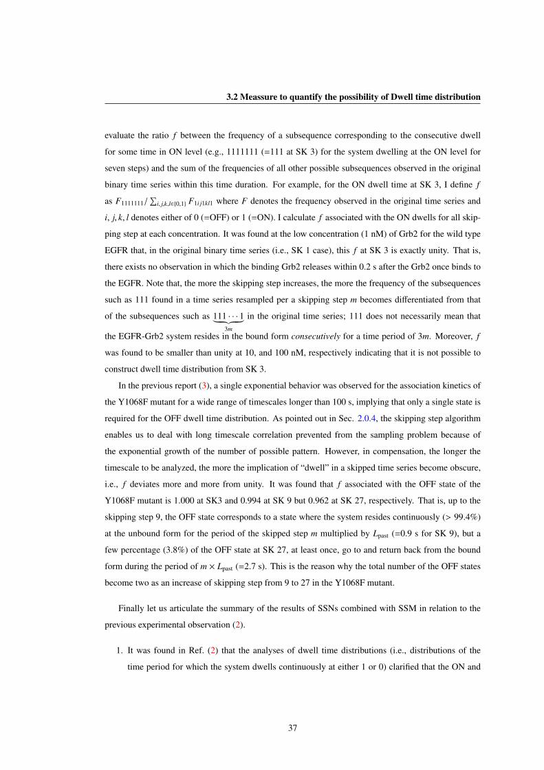
3.2 Meassure to quantify the possibility of Dwell time distribution

evaluate the ratio f between the frequency of a subsequence corresponding to the consecutive dwell

for some time in ON level (e.g., 1111111 (=111 at SK 3) for the system dwelling at the ON level for

seven steps) and the sum of the frequencies of all other possible subsequences observed in the original

binary time series within this time duration. For example, for the ON dwell time at SK 3, I define f

as F1111111/∑

i, j,k,l∈{0,1} F1i j1kl1 where F denotes the frequency observed in the original time series and

i, j, k, l denotes either of 0 (=OFF) or 1 (=ON). I calculate f associated with the ON dwells for all skip-

ping step at each concentration. It was found at the low concentration (1 nM) of Grb2 for the wild type

EGFR that, in the original binary time series (i.e., SK 1 case), this f at SK 3 is exactly unity. That is,

there exists no observation in which the binding Grb2 releases within 0.2 s after the Grb2 once binds to

the EGFR. Note that, the more the skipping step increases, the more the frequency of the subsequences

such as 111 found in a time series resampled per a skipping step m becomes differentiated from that

of the subsequences such as 111 · · · 1︸ ︷︷ ︸3m

in the original time series; 111 does not necessarily mean that

the EGFR-Grb2 system resides in the bound form consecutively for a time period of 3m. Moreover, f

was found to be smaller than unity at 10, and 100 nM, respectively indicating that it is not possible to

construct dwell time distribution from SK 3.

In the previous report (3), a single exponential behavior was observed for the association kinetics of

the Y1068F mutant for a wide range of timescales longer than 100 s, implying that only a single state is

required for the OFF dwell time distribution. As pointed out in Sec. 2.0.4, the skipping step algorithm

enables us to deal with long timescale correlation prevented from the sampling problem because of

the exponential growth of the number of possible pattern. However, in compensation, the longer the

timescale to be analyzed, the more the implication of “dwell” in a skipped time series become obscure,

i.e., f deviates more and more from unity. It was found that f associated with the OFF state of the

Y1068F mutant is 1.000 at SK3 and 0.994 at SK 9 but 0.962 at SK 27, respectively. That is, up to the

skipping step 9, the OFF state corresponds to a state where the system resides continuously (> 99.4%)

at the unbound form for the period of the skipped step m multiplied by Lpast (=0.9 s for SK 9), but a

few percentage (3.8%) of the OFF state at SK 27, at least once, go to and return back from the bound

form during the period of m × Lpast (=2.7 s). This is the reason why the total number of the OFF states

become two as an increase of skipping step from 9 to 27 in the Y1068F mutant.

Finally let us articulate the summary of the results of SSNs combined with SSM in relation to the

previous experimental observation (2).

1. It was found in Ref. (2) that the analyses of dwell time distributions (i.e., distributions of the

time period for which the system dwells continuously at either 1 or 0) clarified that the ON and

37

3. RESULT AND DISCUSSION

OFF states must contain multiple states, though the non-Markovian properties of the EGFR-Grb2

recognition kinetics of ON/OFF time series could not be simply described by the multiple states

whose number was evaluated from the non-single exponential features of the dwell time distribu-

tions. It has been discussed in the experiments (2) that the appearance of multiple states is due to

either the conformational fluctuations of EGFR or the different binding sites between the EGFR

with the Grb2. In our current SSN scheme combined with the SSM, the extraction of the states

is based not on the dwell time distribution but on the pattern buried in the time series, multiple

states are naturally detected for the EGFR-Grb2 system, with encoding memory effects.

2. Our formula reproduces their autocorrelation function for a wide range of timescales up to about

3 s, and the topographical structure of the SSNs changes as an increase of the timescale: while

the corresponding SSN is rather simple at the short timescale (0.033 to 0.1 s), the SSN at the

longer timescales (0.1 s to ∼ 3 s) becomes complex for the elucidation of hierarchically organized

kinetics appearing at the longer timescale in the wild type and the Y1068F mutant of EGFR.

This is interpreted as being captured in some super basin to attain stationary behavior in the short

timescale. One possible scenario to make the SSN more complex as an increase of the timescale

is that partial interactions between the wild type EGFR and the Grb2 occurring faster than the

experimental time resolution (2). Such partial interactions possibly change the conformation of

proteins, and conformational memory produced after dissociation can affect the reduction of the

on-rates, which leads to the structural change of SSNs.

3. It is found that, when the system once visits the unbound form of EGFR· · ·Grb2, the system ap-

proximately loses history or memory. This manifests the existence of heterogeneity of molecular

memory, i.e., dependent on paths or states, the degree to what extent the system possesses the

memory can be different. The interpretation is that the conformational dynamics of the unbound

EGFR relax fast enough before the binding of the next Grb2. On the contrary, the bound states of

the EGFR-Grb2 system keep splitting as L past increases, suggesting slower relaxation dynamics

for the bound EGFR-Grb2 complex. In the Y1068F mutant, the bound state does not split up to

0.133 s (i.e., Lpast = 3) in Fig. 3.8, indicating the dynamics of the bound state relax faster than

those of the wild type.

4. In the experiments, the Y1068F mutant showed non-exponential features in the dissociation ki-

netics at all concentration similarly to the wild type (2). However, the association kinetics (= the

dwell time distribution at the unbound form) at 1 nM concentration showed that it is approximated

by a single exponential kinetics for a wide range of timescales (2, 3). The SSNs for the Y1068F

38

3.2 Meassure to quantify the possibility of Dwell time distribution

mutant is interpreted to reflect such complexity of kinetics: the SSNs for the Y1068F mutant has

effectively a single OFF state up to the timescale of ∼ 1.2 s at 1 nM (See Fig. 3.7), while at 10 nM

the single OFF state found at SK 1 splits into two and more at the larger SK 9 and 27 (See also

Fig. 5.6) in Appendix.

39

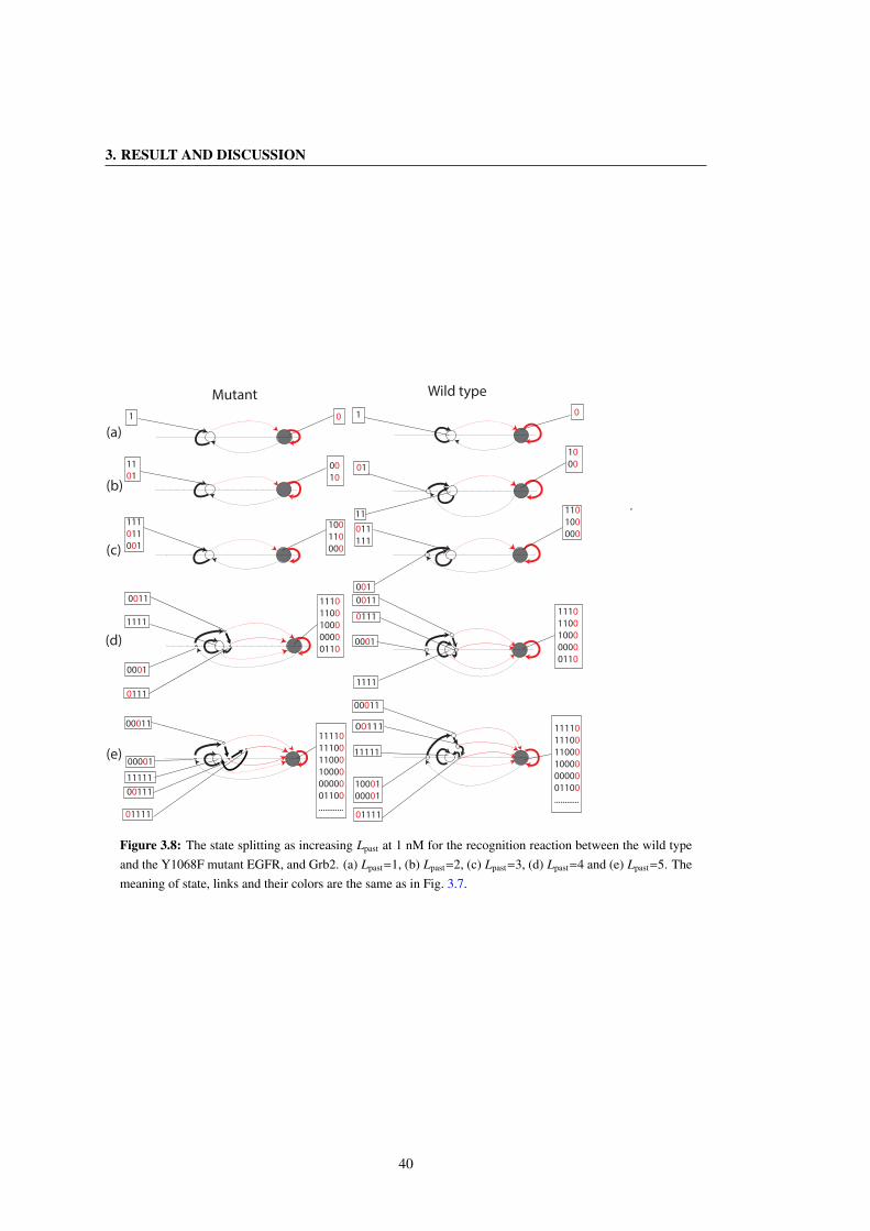
3. RESULT AND DISCUSSION

00001

Mutant Wild type

1 01 0

01

11

10

0000

10

11

01

111

011

001

100

110

000

110

100

000011

111

001

0011

0111

11110

11100

11000

10000

00000

01100

............

00011

11111

01111

10001

00001

00111

1110

1100

1000

0000

01100001

0001

1111

0111

0011 1110

1100

1000

0000

0110

11110

11100

11000

10000

00000

01100

............

11111

00011

00111

01111

1111

(a)

(b)

(c)

(d)

(e)

Figure 3.8: The state splitting as increasing Lpast at 1 nM for the recognition reaction between the wild typeand the Y1068F mutant EGFR, and Grb2. (a) Lpast=1, (b) Lpast=2, (c) Lpast=3, (d) Lpast=4 and (e) Lpast=5. Themeaning of state, links and their colors are the same as in Fig. 3.7.

40

4

Conclusion

4.1 Conclusion and Perspectives

In this thesis I have presented a novel scheme to extract the multiscale state space network that takes

into account multiple nature of the states unseen in measurements and non-Markovianity of the process

solely from SM time series. The crux is the combination of a nonlinear time series analysis recently

developed on the basis of information theory (1, 39, 40, 52, 54, 67) with the SSM. I also derived the exact

formula for the autocorrelation function of the symbolic time series. In this thesis, I demonstrated the

potential of my theory by applying to the ON/OFF SM time series of the recognition kinetics between

the wild type and the Y1068F mutant of EGFR and Grb2 for an in vitro reconstituted system at all

concentrations of Grb2 (2, 3). Mathematically there is no difficulty to generalize this theory into non-

binary time series having more than two symbols. However, as the number of symbols increases much

more than two, the statistical accuracy becomes worse. Improper symbolization may also lose the

essential information to be retrieved.

I have also derived the exact formula for the dwell time distribution for binary time series (the ex-

tension to non-binary time series is straightforward). However, a drawback of SSM is that it is not

straightforward to relate the multiscale kinetics captured by the SSNs directly to the dwell time distri-

bution. So, I have quantified the possibility to replicate the dwell time up to a certain skipping step from

the EGF-Grb2 recognition kinetics of ON/OFF time series. It needs more mathematical study to recover

this problem. One of the possible solution is to combine all networks for different skipping steps and

construct one network.

Appropriate symbolization of time series depends on the experimental setting. In general, the ob-

served time traces are contaminated by several sources of extrinsic and intrinsic noises. It is of crucial

41

4. CONCLUSION

importance to extract the actual time trace of a physical quantity (e.g., interdye distance) desired for the

further analysis from a raw data (e.g., photon arrival times at the donor and acceptor channels) (73).

An accurate assignment of ON/OFF levels is very difficult due to the intrinsic and extrinsic noises in

SM fluorescence measurements. Also, the distribution of on-level depends on the choice of binning

time and threshold level (74). Recently, it was shown that the existence of dynamic disorder of single

enzymatic turnover reactions depends on how one assigns the ON/OFF levels and the most widely used

binning and thresholding approach may yield a misleading interpretation (61). In addition, the choice

of a bin width introduces an artificial time scale to the measurement and raised the possibility of missed

transitions due to information lose in each bin (75) and also a hard threshold is vulnerable to detect of

false transitions of state to state. Yang group applied a change point analysis method, to analyze the

statistics of switching among different levels, which avoids binning the data. Nonetheless, this method

involves various explicit and implicit assumptions. So, in my ongoing project, I am investing raw data to

identify the change point of time series i.e. assigning “on-off” trajectories based on CUSUM and boot-

strap method. These two methods are more flexible in order to deal with low intensity fluctuations at

the background (noise) compared with other existing methods. Furthermore, these methods are simpler

to handle any kind of data set. Since some subsequences involving one step transitions in the ON/OFF

time series were removed from the analyses (2), it is desired to confirm how such removals would affect

in the analyses based on above change point detection method.

Recently, it is found that conformation fluctuations are not only the reasons for concentration depen-

dency on rate constant of association process (47) for this EGFR-Grb2 system. To identify the origin that

may induce Grb2 dependence on this process, it is better to investigate more facts by using appropriate

method, such as flux balance analysis (FBA) (76) by decomposing the transition matrix of SSN.

It should also be noted that the SSN scheme groups a set of past subsequences (into a single state)

whose transition probability distributions are regarded as identical within an error tolerance determined

by the significance level. The grouping and resultant states depend on this significance level and even

if two past subsequences are grouped into a certain state for a specific significance level, it might not

be the case for another significance level. Therefore, a SSN constructed for a certain significance level

may mislead the precise interpretation concerning the underlying SSN. Therefore, the visualization of

the SSN projected onto the metric space that reflects the proximity of transition probability distribution

is very crucial to capture the essence of the network structure.

In the literature, a state is often regarded as a conformation or, a set of conformations or, more

generally, a set of static conformation composed of an energy basin. Importantly, when the process is

non-Markovian, in order to keep such a static concept of states, one needs to introduce the so-called

42

4.1 Conclusion and Perspectives

memory kernel in an ad hoc fashion. In the SSN construction, instead of introducing the memory kernel

whose physical interpretation is absent, the concept of states become “dynamic", i.e., the sequence of

snapshots of conformation changes. From my standpoint, compared to introducing ad hoc memory

kernel which is normally fitted to the experimentally observed autocorrelation, the concept of states in

SSN is regarded as showing a solid connection to conformations (is not static but dynamic fashion).

However, direct connections between the high dimensional protein conformations and states obtained

from the SSN analysis may not be established solely based on the information of a one-dimensional

time series. This limitation is inherent to most of all measurements, but I expect that a systematic survey

of the dependence on several amino acid residue mutations provides more concrete identification of the

state in relation to the identity of the role of amino acid residues. This may be regarded as ϕ value

analysis of protein folding kinetics to infer the energy landscape in the framework of SM biology.

The nonstationary features and the timescale dependence of the constructed networks are the natural

consequence arising from the property of the system in question, whenever states are defined along the

time series. One of the alternative data-driven approaches to construct a network is to utilize dwell-time

time series, which is the series of the consecutive dwell times at the individual levels such as ON and

OFF (46). It is interesting to compare the results of these complimentary approaches as one of the

forthcoming subjects.

43

4. CONCLUSION

44

5

Appendix

5.0.1 Overview of EGFR and EGFR family

Cell signaling is a part of a complex system of communication, governs basic cellular activities and

coordinates cell actions. Cells interact with extracellular stimulus via the membrane bound receptors e.g.

receptor tyrosine kinases (RTKs (See Fig. 5.2)). These receptors for most growth factors like epidermal

growth factor (EGF) transfer signal to tyrosine-specific protein kinases combined with adaptor protein

in cytoplasm. They all follow a critical signaling pathway, which is directed from the cell surface to

the nucleus. The binding of a growth factor (EGF) to its tyrosine kinase receptor (i.e EGFR) protein on

the plasma membrane results as autophosphorylation and activate the Ras/Raf/MAPK cascade (6, 77).

This cascade passes the signal to the nucleus through phosphorylation of transcription factors, leading to

DNA synthesis and cell division (78, 79). The responds of this signal transduction are, in form of robust

functions in the cell such as thermally fluctuation (i.e., chemical reactions in time and space scales),

reordering the environment inside the cell.

A class of RTKs belonging to the family of ErbB plays a pivotal role in cell cycle. ErbB family

consists of four receptors namely ErbB1(which known as EGFR), ErbB2 (HER2), ErbB3 (HER3), and

ErbB4 (HER4) which are variously activated by signal molecules (4). All four members have in common

an extracellular ligand-binding domain, a single hydrophobic transmembrane domain, and a cytoplas-

mic region, which contains a highly conserved tyrosine kinase domain and C-terminal tail (Fig. 5.1).

However, tyrosine kinase of ErbB3 is not active due to the amino acids within the kinase domain (80).

The extracellular domains are less conserved among the four (5).

Dimerization and phosphorylation of the epidermal growth factor (EGF) receptor (EGFR) are the

initial and essential events of EGF-induced signal transduction. EGFRs can form dimer on the cell sur-

face independent of ligand binding (80). It has been reported that the binding of EGF to an EGFR dimer

45

5. APPENDIX

Y 992

Y 1045

Y 1068Y 1143

Y 1173

Ex

tra

cell

ula

r R

eg

ion

Trancemembrane

Juxtamembrane

Tyrosine Kinase

Sites of tyrosine

Phosphorylation

Downstream

signaling molecule

Intr

ace

llu

lar

Re

gio

n

Cell

Cytosol

Cytoplasmic

domain

Cysteine-rich domain

Cysteine-rich domain

165

1

310

480

620

643

685

953

1183

Figure 5.1: Basic Structure of EGFR demonstrating relevant domains. (I) The extracellular region con-sists of four domains ( two of them are rich in cysteine). (II) Transmembrane domains. (III) The intracellulardomains:(1) juxtamembrane domain; (2) tyrosine kinase domain; (3) regulatory region domain. The phospho-rylation of several substrates by the tyrosine kinase domain of the EGFR receptor is responsible for activatingthe various signaling cascades that are shown in the tail of the EGFR in the cytosol. This figure was publishedfrom Refs. (4, 5).

46

5.1 Persistence of Markovian state with different skipping times

is stronger than EGF binding of an EGFR monomer (80). Dimerized EGFR induces autophosphory-

lation of tyrosine residues in the c-terminal of EGFR by its own kinase domain. The resulting phos-

phorylated tyrosine residues serve as binding sites for molecules containing Src homology 2 domains

and initiate intracellular signaling cascades linked to versatile cellular responses, including regulation

of gene expression (4). These dimerized complexes are formed before second EGF molecule binds sug-

gesting bivalent binding of EGF. “Twisting” model was proposed for this dimerization at where dimer

EGFR performed as twister after activated by EGF (22). The cytoplasmic domain of EGFR contains a

long tail of amino acids, and it has been shown that this domain causes a conformational change upon

phosphorylation of tyrosine resides, which could affect interactions with cytoplasmic binding proteins.

5.0.2 Grb2

Adaptor proteins, known as secondary messenger of the signal transdruction, have a variety of protein-

binding modules which link to protein-binding partners together and initiate the larger signaling com-

plexes. There are many types of adaptor proteins in cytoplasm which interact signaling proteins in the

cell signal transduction process. MyD88, Grb2 and SHC1 are famous adaptor proteins of human cell.

Grb2 is an adaptor protein involved in signal transduction for MAPK/ERK pathway (See Fig. 5.2). It

contains one SH2 domain and two SH3 domains. These two SH3 domains direct complex formation

with proline-rich regions of other proteins, and SH2 domain binds tyrosine phosphorylated sequences.

In this thesis, one important issue is to investigate how growth factor receptors (EGFR) interact with

adaptor protein (Grb2) in the cytoplasm and initiate signaling in cells i.e., from the outside of a cell,

receptors activate a different set of cellular signaling leading to different outcome. The conformational

changes in EGFR as a result the kinetic properties between Grb2 and intact EGFR could be complex

and is still not clear (2).

5.1 Persistence of Markovian state with different skipping times

Here we show that if there exists only one unique state for a given symbol at SK 1, then there also exists

only one unique state for the same symbol for arbitrary skipping time. Without loss of generality, we

provide the proof for the case of SK 2. The generalization to the cases with arbitrary skipping time is

straightforward. Mathematically, we show that if we have at SK 1

P(si1 |s∗i0 si−1 si−2 · · · ) = P(si1 |s∗i0 ) = P(si1 |S ∗I0) (5.1)

47

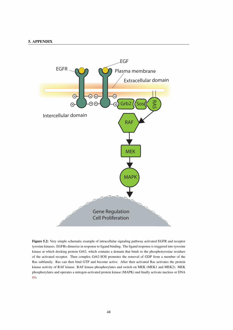
5. APPENDIX

Sos

RA

SGrb2

Intercellular domainP

P P

EGFR

EGF

PP

PP

Plasma membrane

MEK

MAPK

RAF

Extracellular domain

P

Gene Regulation

Cell Proliferation

Figure 5.2: Very simple schematic example of intracellular signaling pathway activated EGFR and receptortyrosine kinases. EGFRs dimerize in response to ligand binding. The ligand response is triggered into tyrosinekinase at which docking protein Grb2, which contains a domain that binds to the phosphotyrosine residuesof the activated receptor. Then complex Grb2-SOS promotes the removal of GDP from a member of theRas subfamily. Ras can then bind GTP and become active. After then activated Ras activates the proteinkinase activity of RAF kinase. RAF kinase phosphorylates and switch on MEK (MEK1 and MEK2). MEKphosphorylates and operates a mitogen-activated protein kinase (MAPK) and finally activate nucleus or DNA(6).

48

5.1 Persistence of Markovian state with different skipping times

where S ∗I0is the only state associated with the given symbol s∗i0 , then for any skipping time, e.g. SK 2,

we also have

P(si2 |s∗i0 si−2 si−4 · · · ) = P(si2 |s∗i0 ) (5.2)

that implies the existence of one unique state containing all the possible subsequences · · · si−4 si−2 s∗i0 for

SK 2. It is noted that Eq. 5.2 and the first equal sign in Eq. 5.1 indicate that once the system visits

the symbol s∗i0 , the transition probabilities to the future symbol becomes Markovian regardless of the

skipping time and therefore “resets” the memory of the system as discussed in the main text.

We first show that if Eq. 5.1 holds, we also have

P(si2 si1 |s∗i0 si−1 si−2 · · · ) = P(si2 si1 |s∗i0 )

= P(si2 si1 |S ∗I0).

(5.3)

This means that the Markovian property also holds in predicting more than one future symbol. By using

the chain rules of the transition probability, we have

P(si2 si1 |s∗i0 si−1 si−2 · · · )

=P(si2 |si1 s∗i0 si−1 · · · )P(si1 |s∗i0 si−1 · · · )

=P(si2 |si1 s∗i0 si−1 · · · )P(si1 |s∗i0 ),

(5.4)

where Eq. 5.1 is used in the last equality. Since both the subsequences · · · si−2 si−1 s∗i0 and s∗i0 can be

represented by the state S ∗I0according to Eq. 5.1, we then have P(si2 |si1 s∗i0 si−1 · · · ) = P(si2 |si1 S ∗I0

) =

P(si2 |si1 s∗i0 ). As a result, Eq. 5.4 becomes

P(si2 si1 |s∗i0 si−1 si−2 · · · )

=P(si2 |si1 s∗i0 si−1 · · · )P(si1 |s∗i0 )

=P(si2 |si1 S ∗I0)P(si1 |s∗i0 )

=P(si2 |si1 s∗i0 )P(si1 |s∗i0 )

=P(si2 si1 |s∗i0 ).

(5.5)

Next by summing over the symbol si1 in Eq. 5.3, we can easily obtain

P(si2 |s∗i0 si−1 si−2 · · · ) = P(si2 |s∗i0 ) (5.6)

49

5. APPENDIX

Now we are ready to show the equality in Eq. 5.2

P(si2 |s∗i0 si−2 si−4 · · · )

=P(si2 s∗i0 si−2 si−4 · · · )P(s∗i0 si−2 si−4 · · · )

=

∑si−1 si−3 ··· P(si2 s∗i0 si−1 si−2 si−3 · · · )

P(s∗i0 si−2 si−4 · · · )

=

∑si−1 si−3 ··· P(si2 |s∗i0 si−1 si−2 si−3 · · · )P(s∗i0 si−1 si−2 · · · )

P(s∗i0 si−2 si−4 · · · )

=

∑si−1 si−3 ··· P(si2 |s∗i0 )P(s∗i0 si−1 si−2 · · · )

P(s∗i0 si−2 si−4 · · · )=P(si2 |s∗i0 )

(5.7)

where Eq. 5.6 is used in the second last equal sign.

5.1.1 Result of Lpast and significance Level

In this work, the construction of SSN from time series is performed by an algorithm developed by

Klinkner and Shalizi (62). In order to assign the past subsequences of a time series to each state, the

algorithm uses the Kolmogorov-Smirnov test (53) to compare the transition probabilities (from the past

subsequences to the future value) up to a desired significance level (α). There is only one physical

parameter required to be determined in the algorithm, namely, the length of the past subsequence, Lpast,

which should be long enough to capture statistical correlation presented in the time series. In general,

one extracts the converged SSNs using the algorithm by checking if the statistical complexity (i.e. the

Shannon entropy of residential probability of the states, −∑I P(S I) log P(S I)) of the SSN converges

with respect to Lpast.

On the other hand, the significance level (α) is the probability that two subsequences are mistakenly

assigned to different states even though they should belong to the same state. The choice of a very small

value of α tends to assign subsequences to different states only when their transition probabilities to the

future values are significantly different and, therefore, results in fewer states. On the other hand, the

assignment of subsequences into different states is less strict if a large value of α is used. In our SSN

construction, we worked with the range of α values in which the subsequences assignment is insensitive

to the change of α.

In Fig. 5.3(a), we show the change of the statistical complexity associated with the time series for

the three states model with SK 1. We can see that the converged SSN is given at Lpast = 2. For time

series with long correlation time which requires a large Lpast to reach the converged SSN, one in general

suffers from the sampling problem since the number of past subsequences grows exponentially with

50

5.1 Persistence of Markovian state with different skipping times

Stat

isti

cal c

om

ple

xity

L

(b)(a)

0 2 4 6 8 100.4

0.5

0.6

0.7

0.8

0.9

1.0

0 2 4 6 8 100.10

0.12

0.14

0.16

0.18

0.20

(d)Lpast Lpast

Lpast Lpast

(c)

0 2 4 6 8 100.30

0.35

0.40

0.45

0.50

2 4 6 8 100.0

0.5

1.0

1.5

Figure 5.3: The statistical complexity versus Lpast for different significance levels α in the Kolmogorov-Smirnov test for SK 1, with α = 0.1, 0.05, 0.01, 0.005 and 0.001 for both (a) the three states model (Sec. 3.1)and the association and dissociation reaction between the wide type EGFR and Grb2 at (b) 1 nM, (c) 10 nM,and (d) 100 nM. Different colors correspond to different values of α: red 0.1, green 0.05, pink 0.01, black0.005, and blue 0.001. In (a) Lpast = 2 results in a converged SSN for the three states model. In the wild typeEGFR case, Lpast = 3 was chosen to yield the approximate (local) convergent network for (b) 1 nM, (c) 10 nMand (d) 100 nM.

51

5. APPENDIX

Lpast. In this case, we resample our time series and apply the skipping step method as discussed in the

main text. In the case of the three states model, we construct the converged SSNs for SK 1, SK 3, SK

9 and SK 27 with Lpast equal to 2, 1, 0 and 0, respectively. In the EGFR case for all concentration, the

statistical complexity increases very slightly and gradually (See, e.g., Fig. 5.3(b)-(d)) and it is difficult to

conclude any convergent Lpast. However, in the case of the wild type and the Y1068F mutant of EGFR

we found some locally convergent network at Lpast equal to 2 or 3. Hence, we chose Lpast = 3 for all

SSNs to be analyzed.

5.1.2 Results of autocorrelation of the wild type and the Y1068F mutant at 10and 100 nM Grb2

Au

toco

rre

lati

on

Time(s)

0.1 0.2 0.5 1.0 2.0 5.0

0.080

0.060

0.040

0.020

Wild type

Mutant

0.03

Figure 5.4: Autocorrelation for the ON/OFF time series of the association and dissociation processes betweenthe wild type and the Y1068F mutant at 10 nM concentration of Grb2. See the caption of Fig. 3.6.

52

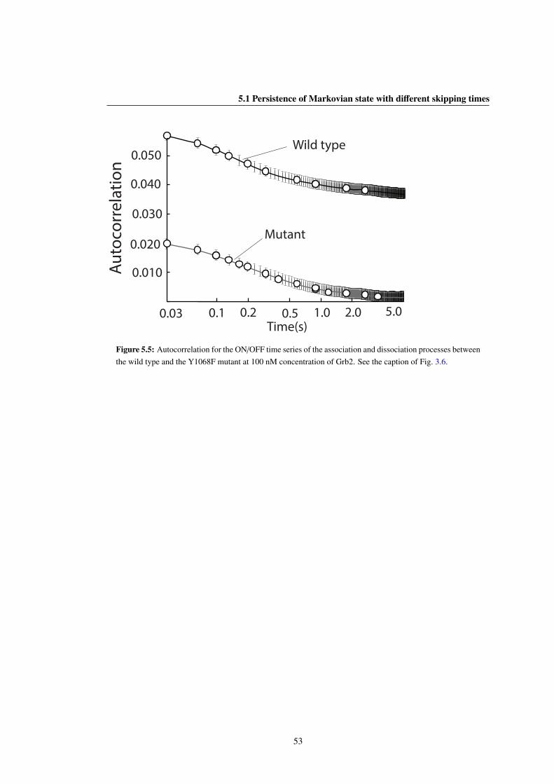
5.1 Persistence of Markovian state with different skipping times

Au

toco

rre

lati

on

Wild type

Mutant

0.1 0.2 0.5 1.0 2.0 5.0Time(s)

0.050

0.040

0.030

0.020

0.010

0.03

Figure 5.5: Autocorrelation for the ON/OFF time series of the association and dissociation processes betweenthe wild type and the Y1068F mutant at 100 nM concentration of Grb2. See the caption of Fig. 3.6.

53

5. APPENDIX

Mutant Wild type

SK 1

SK 3

SK 9

SK 27

000

110

100

011

111

001

000

110

100

111

001

011

000

100111

011

001010

110

101

010

110111

001

011

101

000

100

011

111

001

101110

010

000

100

110

010

111

101

001

100

011000

000

100

010

110

111

001

101

011

111

001

011

101

000

100

010

110

Figure 5.6: The SSNs of the wild type (right) and the Y1068F mutant (left) at 10 nM concentration of Grb2for different skipping steps (SK 1, 3, 9, and 27 from the top to the bottom). See also the caption of Fig. 5.6 inthe main text.

54

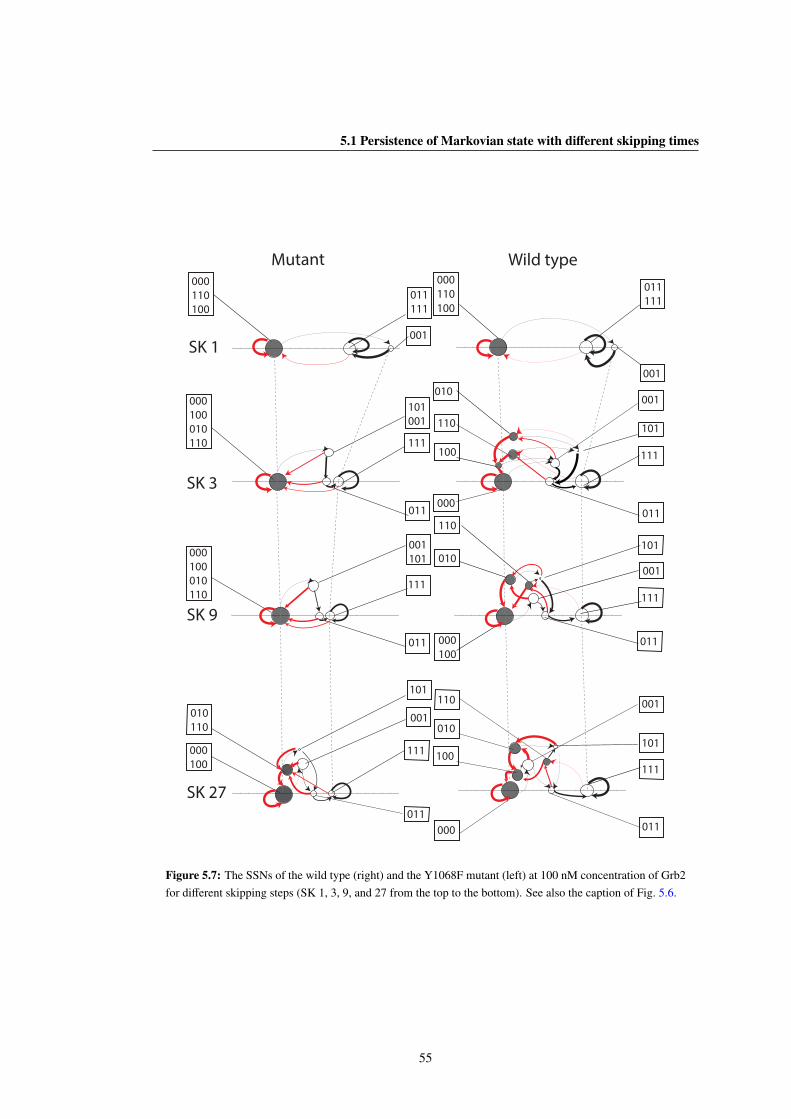
5.1 Persistence of Markovian state with different skipping times

Mutant Wild type

SK 1

SK 3

SK 9

SK 27

000

110

100

011

111

001

000

100

010

110 111

011

101

001

111

011

000

100

010

110

001

101

000

100

011

111

001

101

010

110

000

110

100

011

111

001

010

111

101

001

000

110

011

100

000

100

010

110

001

111

011

101

110

111

001

011000

010

100101

Figure 5.7: The SSNs of the wild type (right) and the Y1068F mutant (left) at 100 nM concentration of Grb2for different skipping steps (SK 1, 3, 9, and 27 from the top to the bottom). See also the caption of Fig. 5.6.

55

5. APPENDIX

5.1.3 The Visualization of the underlying SSNs of the wild type and the Y1068Fmutant at 10 and 100 nM Grb2 and their lifetime constants

Table 5.1: The lifetime constants of the wild type EGFR at all concentration of Grb2 for each state spacenetwork. The lifetime constants are calculated from Eq. (5) (in the main text) and their weights are shown inparentheses.

[Grb2] SK 1 SK 3 SK 9 SK 27

1 nM 0.0037 (2%) 0.028 (14%) 0.15 (14%) 0.023 (1%)0.37 (98%) 0.58 (86%) 1.29 (86%) 0.61 (39%)

0.69 (25%)3.50 (35%)

10 nM 0.007 (8%) 0.06 (1%) 0.14 (0.02%) 0.47 (1%)0.43 (92%) 0.07 (14%) 0.18 (1.18%) 0.59 (2%)

0.69 (85%) 0.28 (26%) 0.92 (33%)0.30 (14%) 1.09 (18%)

2.40 (58.8%) 9.95 (46%)100 nM 0.004 (1%) 0.088 (0.6%) 0.12 (14%) 0.55 (14%)

0.70 (99%) 0.055 (9.2%) 0.3 (6%) 0.62 (14%)0.086 (4.18%) 5.87 (80%) 1.12 (3%)

0.21 (0.02%) 1.14 (5%)1.65 (86%) 21.0 (64%)

Table 5.2: The lifetime constants of the Y1068F mutant EGFR at all concentration for each state spacenetwork (The unit is of second). See also the caption of Table 5.1.

[Grb2] SK 1 SK 3 SK 9 SK 27

1 nM 0.56 (100%) 0.02 (4%) 0.10 (0.97%) 0.42 (6%)0.92 (96%) 0.12 (0.03%) 0.47 (2%)

1.46 (99%) 2.04 (92%)10 nM 0.004 (0.99%) 0.04 (15%) 0.140 (8%) 0.41 (35%)

0.32 (99.01%) 0.05 (2%) 0.145 (5%) 0.42 (35%)0.50 (83%) 1.0 (87%) 0.45 (2%)

2.87 (28%)100 nM 0.004 (1%) 0.03 (6%) 0.27 (13%) 1.30 (8%)

0.29 (99%) 0.42 (94%) 2.43 (87%) 1.40 (26%)7.82 (66%)

56

References

[1] C. B. Li, H. Yang and T. Komatsuzaki, Proc. Natl. Acad. Sci. U.S.A., 2008, 105, 536–541.

[2] M. Morimatsu, H. Takagi, K. G. Ota, R. Iwamoto, T. Yanagida and Y. Sako, Proc .Natl. Acad. Sci.

U.S.A., 2007, 104, 18013–18018.

[3] H. Takagi, M. Morimatsu and Y. Sako, Adv. Chem. Phys., 2012, 146, 195–215.

[4] A. Oyewale, K. F. Mark and S. Ravi, Nat. Clin. Pra. Oncol., 2007, 4, 118–129.

[5] Y. Yarden and Sliwkowski, Nat. Rev., 2001, 2, 127–137.

[6] B. Alberts, D. Bray, K. Hopkin, A. Johnson, J. Lewis, M. Raff, K. Roberts and P. Walter, "Essentail

Cell Biology", NEW YORK AND LONDON: Garland Science, 2004.

[7] R. Zwanzig, Nonequilibrium Statistical Mechanics, Oxford University Press, New York, NY, 2001.

[8] J. Wang and P. Wolynes, Phys. Rev. Lett., 1995, 74, 4317–4320.

[9] S. L. Yang and J. S. Cao, J. Phys. Chem B, 2001, 105, 6536–6549.

[10] Y. J. Jung, E. Barkai and J. R. Silbey, J. Chem. Phys, 2002, 117, 10980–10995.

[11] X. S. Xie, J. Chem. Phys., 2002, 117, 11024–11032.

[12] G. S. Harms, G. Orr, M. Montal, B. D. Thrall, S. D. Colson and H. P. Lu, Biophys. J., 2003, 85,

1826–1838.

[13] H. Lu, L. Xun and X. Xie, Science, 1998, 282, 1877–1882.

[14] X. Tan, P. Nalbant, A. Toutchikine, D. Hu, E. Vorpagel, K. Harn and H. Lu, J. Phys. Chem. B.,

2004, 108, 737–744.

[15] V. Bierbaum and R. Lipowsky, PLOS ONE, 2013, 8, 55366.

57

REFERENCES

[16] P. E. Wrigth and H. J. Dyson, J. Mol. Biol, 2001, 293, 321–331.

[17] O. A. Van, P. Blainey, D. Crampton, C. Richardson, T. Ellenberger and X. Xie, Science, 2003, 301,

1235–1238.

[18] L. Edman and R. Rigler, Proc. Natl. Acad. Sci. U.S.A., 2000, 97, 8266–8271.

[19] X. Zhuang, H. Kim, M. J. B. Pereira, H. P. Babcock, N. G. Walter and S. Chu, Science, 2002, 296,

1473–1476.

[20] Y. Arai, A. Iwane, T. Wazawa, H. Yokota, Y. Ishii, T. Kataoka and T. Yanagida, Biochem. Biophys.

Res. Commun., 2006, 343, 809–815.

[21] X. Michalet, S. Weiss and M. Jaeger, Chem. Rev., 2006, 106, 1785–1813.

[22] Y. Teramura, J. Ichinose, H. Takagi, K. Nishida, T. Yanagida and Y. Sako, EMBO. J., 2006, 25,

4215–4222.

[23] W. Xu, J. S. Kong and P. Chen, PhysChemChemPhys., 2008, 111, 2767–2778.

[24] K. Jacob, Rosenstein, R. Siddharth, R. Jared and L. S. Kenneth, Nano. Lett., 2013, 13, 2682–2686.

[25] B. Hille, Sinaure Associates: Sunderland, MA, 2001, 13, 2682–2686.

[26] Y. Jai, D. S. Talaga, W. L. Lau, H. S. M. Lu, W. F. DeGrado and R. M. Hochtrasser, Chem. Phys.,

1999, 247, 69–83.

[27] D. S. Talaga, W. L. Lau, H. Roder, J. Y. Tang, Y. W. Jia, W. F. DeGrado and R. M. Hochstrasser,

Proc. Natl. Acad. Sci. U.S.A., 2000, 97, 13021–13026.

[28] D. S. . Talaga, Y. Jia, M. A. Bopp, A. Sytnik, W. A. DeGrado, R. J. Cogdell and R. M. Hochstrasser,

Springer Series in Chemical Physics, 2001, 67, 313–325.

[29] E. Mei, J. Tang, J. M. Vanderkooi and R. M. Hochstrasser, J. Am. Chem. Soc., 2003, 125, 2730–

2735.

[30] B. Schuler, ChemPhyChem., 2005, 6, 1206–1220.

[31] X. S. Xie and J. K. Trautman, Annu. Rev. Phys. Chem., 1998, 49, 441–480.

[32] T. Ha, A. Y. Ting, J. Liang, W. B. Caldwell, A. A. Deniz, D. S. Chemla, P. G. Schultz and S. Weiss,

Proc. Natl. Acad. Sci. U.S.A., 1999, 96, year.

58

REFERENCES

[33] A. S. JR, J. App. Econometr., 1993, 8, 63–84.

[34] S. Kondo and T. Miura, Science, 2010, 329, 1616.

[35] M. Andrec, R. M. Levy and D. S. Talaga, J. Phys. Chem. A., 2003, 107, 7454–7464.

[36] T. C. Messina, H. Kim, J. T. Giurleo and D. S. Talaga, J. Phys. Chem. B., 2006, 110, 16366–16376.

[37] S. A. McKinney, C. Joo and T. Ha, Biophys. J., 2006, 91, 1941–1951.

[38] L. R. Rabiner, Proc. IEEE, 1989, 77, 257–289.

[39] C. B. Li, H. Yang and T. Komatsuzaki, J. Phys. Chem. B., 2009, 113, 14,732–14,741.

[40] C. B. Li and T. Komatsuzaki, Extracting the Uderlying Unique Reaction Scheme from a Single-

Molecule Time Series, Springer Science, 2011.

[41] I. V. Gopich and A. Szabo, J. Chem. Phys., 2006, 124, 154712.

[42] K. A. Merchant, R. B. Best, J. M. Louis, I. V. Gopich and W. A. Eaton, Proc. Natl. Acad. Sci.

U.S.A., 2007, 104, 1528.

[43] I. V. Gopich and A. Szabo, J. Phys. Chem. B, 2005, 109, 17683.

[44] A. Baba and T. Komatsuzaki, Proc. Natl. Acad. Sci. U.S.A., 2007, 104, 19297–19302.

[45] O. Flomenbom and R. J. Silbey, Phys.Rev.E, 2007, 76,.

[46] C. B. Li and T. Komatsuzaki, Phys. Rev. Lett., 2013, 111, 058301–5.

[47] J. Yang and E. P. John, J. Chem. Phys., 2012, 136, 244506.

[48] P. Kienker, Proc. R. Soc., 1989, B 236, 269.

[49] H. Wang and H. Qian, J. Math. Phys., 2007, 48, 013303.

[50] D. Fey, R. Findeisen and E. Bullinger, In: Proceedings of the 17th IFAC World Congres. Interna-

tional Federation of Automatic Control, Seoul, Korea, 2008, 313–318.

[51] R. Prado and M. West, Time Series: Modeling, Computation, and Inference, Chapman Hall, CRC

Press Taylor Francis Group, 2010.

[52] J. P. Crutchfield, Nature Phys., 2012, 8, 17–24.

59

REFERENCES

[53] C. R. Shalizi and J. P. Crutchfield, J. Stat. Phys., 2001, 104, 819–881.

[54] J. P. Crutchfield and K. Young, Phys. Rev. Lett., 1989, 63, 105.

[55] H. Yang, G. Luo, P. Karnchanaphanurach, T. M. Louie, I. Rech, S. Cova, L. Xun and X. S. Xie,

Science, 2003, 302, 262–266.

[56] Y. Chook, G. GD., C. Kay, E. Pai and T. Pawson, J. Biol. Chem., 1996, 271, 30472–30478.

[57] M. Lemmon, J. Ladbury, V. MAndiyan, M. Zhou and J. Schlessinger, J. Biol. Chem., 1994, 269,

31653–31658.

[58] D. Cussac, M. Frech and C. P, EMBO. J., 1994, 13, 4011–4021.

[59] T. Sultana, H. Takagi, M. Morimatsu, H. Teramoto, C. B. Li, Y. Sako and T. Komatsuzaki, J. Chem.

Phys., 2013, 139,.

[60] L. P. Watkins and H. Yang, Biophys. J., 2004, 86, 4015.

[61] T. Terentyeva, H. Engelkamp, A. Rowan, T. Komatsuzaki, J. Hofkens, C. B. Li, K. Blank and L. P.

Watkins, ACS Nano, 2012, 6, 346–354.

[62] C. R. Shalizi, http://www.cscs.umich.edu/∼crshalizi/CSSR/, 2003.

[63] P. F. Dunn, "Measurement and Data Analysis for Engineering and Science", New York: Mc-

GrawHill, 2005.

[64] S. E. Kelly, Applied and Computational Harmonic Analysis, 1996, 3, 72–81.

[65] D. I. A. Henry, Analysis of Observed Chaotic Data, Springer, New York, USA., 1996.

[66] S. Teukolsky, W. Vetterling and B. Flannery, Numerical Recipes in Fortran 90, Cambridge Univer-

sity Press, England, 1996.

[67] C. R. Shalizi, K. L. Klinkner and J. P. Crutchfield, Technical Report, Santa Fe Institite,

http://arxiv.org/abs/cs.LG/0210025, 2002.

[68] J. Downward, P. Parker and M. D. Waterfield, Nature, 1984, 311, 483–485.

[69] R. Iwamoto, K. Hanada and E. Mekada, J. Bio. Chem., 1999, 274, 25906–25912.

[70] T. F. Cox and M. A. A. Cox, Multidimensional Scaling, Chapman Hall, London, UK, 2001.

60

REFERENCES

[71] W. J. Krzanowski, J. App. Stat., 2003, 30, 743–750.

[72] Y. Matsunaga, K. S. Kostov and T. Komatsuzaki, J. Phys. Chem. A., 2002, 106, 10898–10907.

[73] L. P. Watkins, H. Chang and H. Yang, J. Phys. Chem. A., 2006, 110, 5191–5203.

[74] H. C. Catherine, S. Orion, X. Wu, R. Purcell, C. Q. M. Drndic and M. Pelton, Nano Lett., 2010,

10, 1692–1698.

[75] L. P. Watkins and H. Yang, J. Phys. Chem. B., 2005, 109, 617–628.

[76] K. Raman and N. Chandra, Brief. Bioinform, 2009, 4, 435–449.

[77] M. H. Cobb, Prog. Biophys. Mol. Biol., 1999, 71, 479–500.

[78] J. Plumpe, Am. J. Physiol. Gastrointest. Liver Physiol., 2000, 278, 173–183.

[79] F. X. Pimentel-Muinos and B. Seed, Immunity, 1999, 11, 783–793.

[80] A. Wells, International Journal of Biochemistry Cell Biology, 1999, 31, 637–643.

iv, 2, 3, 9, 19, 31, 41

61