Instructions for use

Title Spatio-temporal assessment and trend analysis of surface water salinity in the coastal region of Bangladesh

Author(s) Shammi, Mashura; Rahman, Md. Mostafizur; Islam, Md. Atikul; Bodrud-Doza, Md.; Zahid, Anwar; Akter, Yeasmin;Quaiyum, Samia; Kurasaki, Masaaki

Citation Environmental science and pollution research, 24(16): 14273-14290

Issue Date 2017-06

Doc URL http://hdl.handle.net/2115/70649

Rights The final publication is available at Springer via http://dx.doi.org/10.1007/s11356-017-8976-7

Type article (author version)

File Information ESPR_R2 Final Submission.pdf

Hokkaido University Collection of Scholarly and Academic Papers : HUSCAP

1

Spatio-temporal assessment and trend analysis of surface water salinity in the coastal 1

region of Bangladesh 2

Mashura Shammi1,2, Md. Mostafizur Rahman1,3*, Md. Atikul Islam4, Md. Bodrud-Doza1, Anwar 3

Zahid5, Yeasmin Akter6, Samia Quaiyum7, Masaaki Kurasaki3 4

5

1Department of Environmental Sciences, Jahangirnagar University, Dhaka-1342, Bangladesh 6

2Department of Environmental Pollution and Process Control, Xinjiang Institute of Ecology and 7

Geography, Chinese Academy of Sciences, Urumqi-830011, Xinjiang, PR China 8

3Graduate School of Environmental Science, Hokkaido University, Sapporo 060-0810, Japan 9

4Department of Chemistry, Hajee Mohammad Danesh Science and Technology University, 10

Dinajpur-5200, Bangladesh 11

5Ground Water Hydrology, Bangladesh Water Development Board, 72 Green Road, Dhaka 12

1205, Bangladesh 13

6Department of Chemistry, University of Chittagong, Chittagong-4331, Bangladesh 14

7 Dept. of Natural History and Science Faculty of Science, Hokkaido University, Sapporo, Japan 15

16

*Corresponding Author: rahmanmm@juniv.edu Graduate School of Environmental Science,

Hokkaido University, Sapporo 060-0810, Japan

2

Abstract 17

The study was designed to collect water samples over two seasons- wet-monsoon season (n=96) 18

(March-April) and dry-monsoon season (n=44) (September-October) to understand the seasonal 19

variation in anion and cation hydrochemistry of the coastal rivers and estuaries contributing in 20

the spatial trend in salinity. Hydrochemical examination of wet-monsoon season primarily 21

revealed Ca–Mg–HCO3 type (66%) and followed by Na–Cl type (17.70%) water. In the dry-22

monsoon season the scenario reversed with primary water being Na-Cl type (52.27%) followed 23

by Ca–Mg–HCO3 type (31.81%). Analysis of Cl/Br molar ratio vs. Cl (mg/L) depicted sampling 24

area affected by seawater intrusion (SWI). Spatial analysis by Ordinary Kriging method 25

confirmed approximately 77% sample in the dry-monsoon and 34% of the wet-monsoon season 26

had shown SWI. The most saline intruded areas in the wet-monsoon seasons were extreme 27

south-west coastal zone of Bangladesh, lower Meghna River floodplain and Meghna estuarine 28

floodplain and South-eastern part of Chittagong coastal plains containing the districts of 29

Chittagong and Cox’s Bazar adjacent to Bay of Bengal. In addition, mid-south zone is also 30

affected slightly in the dry-monsoon season. From the analyses of data, this study could further 31

help to comprehend seasonal trends in the hydrochemistry and water quality of the coastal and 32

estuarine rivers. In addition, it can help policy makers to obligate some important implications 33

for the future initiatives taken for the management of land, water, fishery, agriculture and 34

environment of coastal rivers and estuaries of Bangladesh. 35

Keywords: seawater intrusion (SWI), estuary, spatial salinity trend, non-parametric test, electric 36

conductivity (EC), Na/Cl molar ratio, Cl/Br molar ratio. 37

38

3

1. Introduction 39

Coastal zones are transition environments, forming the interface between continent and ocean. 40

The effects of human activity on coastal water resources usually reduce the flows of freshwater 41

to estuaries; modifying estuarine mixing processes and extending marine influences further 42

inland (Loitzenbauer and Mendes 2012). Bangladesh is considered as one of the most climate 43

vulnerable countries in the world. In the southern part, it has approximately 710 km coastal line 44

with highly susceptible areas to sea level rise. The coastal area in the southern part covers about 45

32% of total land area of the country (MoWR 2005) and are particularly vulnerable to climate 46

change effects (Bhuiyan and Dutta 2012). Water salinity is regular hazards for many parts of 47

southern Bangladesh. For example, Batiaghata Upazila, Khulna District in south-west coastal 48

region of Bangladesh is the mostly saline affected area, where agriculture activities are mainly 49

dependent on rainfall (Shammi et al. 2016). Previous study on groundwater in south-west part of 50

Bangladesh confirmed the area was dominantly of Na–Cl type brackish water (Halim et al. 2010) 51

due to the seawater influence and hydrogeochemical processes (Bahar and Reza 2010). 52

Anthropogenic and bio-physical factors (e.g., upstream withdrawal of freshwater, cyclones) 53

operating outside the geographical boundary of coastal region of Bangladesh contribute to 54

increasing salinization in the southwest coastal area (Shameem et al. 2014). 55

Nevertheless, it is very difficult to get the actual scenario of hydrochemistry of the coastal river 56

and estuaries due to dynamic mixing. Estuary provides a unique experimental site to understand 57

the effect of monsoonal river discharge on freshwater and seawater mixing (Ghosh et al. 2013). 58

The estuaries that are typically characterized by gradients of ionic strength, pH and 59

concentrations of the suspended particulate matter; provide an ideal environment to study the 60

nature and extent of solute-particle interaction, and the resultant modification of the elemental 61

4

and isotopic fluxes from the rivers to the oceans (Samanta and Dalai 2016). Seawater intrusion 62

(SWI) is a global issue (Werner et al. 2013) in coastal aquifers all over the world and 63

predisposed to the influences of sea level rise and climate change. Surface water such as rivers 64

and canals are impacted similarly by intruding seawater. Here, salinity refers to the total 65

concentration of dissolved inorganic ions in water (Williams and Sherwood 1994) and often 66

measured as electrical conductivity (EC) siemens/meter (Canedo-Arguelles et al. 2013). 67

Temporal and spatial status of water salinity condition in Kumar-Modhumoti River in Gopalganj 68

district showed that during the start of wet-monsoon months (March–April), the conductivity of 69

river water was high due to low rainfall and upstream discharge. Conductivity ranged from 3.5 70

dS/m to 4.0 dS/m, while in the late wet-monsoon months (August−September), the conductivity 71

of river water decreased (0.3–0.4 dS/m) (Shammi et al. 2012). Correlation of river discharge data 72

of Gorai-Madhumati and conductivity of Madhumati River confirmed that salinity level was 73

higher when upstream river inflow was below 500 m3/S (Shammi et al. 2012). 74

In addition, trend analysis provides a view for meteorological, hydrological and climatological 75

variables in past and future time’s changes (Kisi and Ay 2014). The main idea of trend analysis 76

is to detect whether values of data are increasing, decreasing or stable over time. Detection of 77

trend is a complex subject because of characteristics of data (Kisi and Ay 2014). In general, there 78

are different parametric and nonparametric statistical techniques to check the existence or 79

absence of trend in time series analysis and climate change studies but the nonparametric 80

methods are used relatively wider in hydro-meteorological studies (Takeuchi et al. 2003). 81

Nonparametric methods are appropriate for the series that have a significant skew and cannot be 82

fitted with statistical distributions (Niazi et al. 2014). Since then, many nonparametric statistical 83

tests have been developed to determine trends in data series. Mann–Kendall (Mann 1945; 84

5

Kendall 1975) test is one of the best trend detecting methods. This method is suitable for the 85

nonnormal and is not sensitive to observed values. This test has been recommended for detecting 86

trends in environmental time series data by the World Meteorological Organization (Niazi et al. 87

2014). On the otherhand, the Sen’s slope method (Sen 1968) uses a linear model to estimate the 88

slope of the trend (Salmi et al. 2002) with the extent of magnitude at a satisfactory significant 89

level. 90

It is important to determine the possible impacts of sea level rise on salinity to devise suitable 91

adaptation and mitigation measures and reduce impacts of salinity intrusion in coastal cities 92

(Bhuiyan and Dutta 2012). Nevertheless, till to date, there are no studies depicting the actual 93

hydrochemistry related to the salinity condition in the coastal rivers and estuarine waters of 94

Bangladesh. Therefore, this study was designed to collect water samples over two seasons- wet-95

monsoon season and dry-monsoon season, to understand the seasonal variation in anions and 96

cations hydrochemistry of the coastal rivers and esutaries contributing in the spatial trend in 97

salinity. The study was further trailed by time-series analysis of salinity data using Mann–98

Kendall and Sen’s slope test for 13 south-west zone rivers to find salinity trend in of southern 99

regions of Bangladesh followed by existing policy analysis for the management of salinity 100

affected areas. 101

2. Landform and hydromorphological settings 102

Bangladesh occupies an area of 143,998 km2 and has a subtropical humid climate. 103

Geographically, it extends from 20°34′N to 26°38′N latitude and from 88°01′E to 92°41′E 104

longitude. Except the hilly southeast, most of the country is a low-lying plain land (Shahid 2010). 105

The topography of the region is rather flat, and gently sloping towards the Bay of Bengal 106

(Bhuiyan and Dutta 2012). The original morphology and hydrogeology of many low-lying 107

6

coastlands worldwide have been significantly modified over the last century through river 108

diversion, embankment built-up, and large-scale land reclamation projects. This led to a 109

progressive shifting of the groundwater–surface water exchanges from naturally to 110

anthropogenically driven (Da Lio et al. 2015). Hydrology of the coastal plains of Bangladesh 111

presents a complicated interaction of fresh water flow from the upstream, the tides and tidal 112

flows from the Bay of Bengal, tropical cyclones, storm surge and other meteorological effect 113

from the sea and the physiography of the coastal plains (FAO 1985). Understanding the mixing 114

between salt/fresh surface water and groundwater in coastlands is an issue of paramount 115

importance considering the ecological, cultural, and socio-economic relevance of the coastal 116

plains (Da Lio et al. 2015). Low-lying parts of four regions further inland Ganges River 117

floodplain, Old River floodplain comprising Arial Bil and Gopalganj Bil (low-lying lakes), lower 118

Meghna River floodplain and Meghna estuarine floodplain lie sufficiently close to the coast that 119

they could be affected by a rising sea-level at an early date (Brammer 2014a). 120

The physical geography of Bangladesh’s coastal area is more diverse and dynamic than is 121

generally recognised. Failure to recognise this has led to serious misconceptions about the 122

potential impacts of a rising sea-level on Bangladesh with global warming (Brammer 2014b). 123

Estuaries are a transition zone between continental and marine environments and record the 124

complex interaction of these two discrete environments in terms of physical phenomena (e.g. 125

mixing of fresh and saline water, tidal and wave action, sediment transport) and chemistry. They 126

play an important role in understanding the continental input via rivers to the oceans (Ghosh et al. 127

2013). Sea salinity intrusion is a major concern in the southern part of the river system, as the 128

rivers are affected by tides and is an important issue in these rivers. Most of the area is protected 129

with polders against river flooding (Bhuiyan and Dutta 2012). The coastal zone is exposed to the 130

7

risk of tropical cyclones in the wet-monsoon and dry-monsoon seasons, with the associated risk 131

of storm surges in areas close to the coast (Brammer 2014b). 132

133

3. Methodology 134

3.1. Study area 135

The study area for surface water encompasses the coastal south part of the Bengal Basin. The 136

sampling area were selected in the southern part of Bangladesh taking into account the south-east 137

coastal zone to south-west zone of Bangladesh. Geographically, sampling points extended from 138

20°34'N to 23°40'N latitude and from 88°01'E to 92°41'E longitude (Figure 1). Most part of the 139

sampling points lied on the Ganges and Meghna River and their many tributaries and 140

distributaries except south-east part of Chittagong coastal plains and Bay of Bengal. 141

3.2. Description of the available data 142

A various multidisciplinary data are highly needed for the study of sea water intrusion (SWI) to 143

provide reliable results (Trabelsi et al. 2016). Surface water samples were collected in 500 ml 144

plastic bottle for two different seasons March-April 2012, wet-monsoon season (n=96) and 145

September-October 2012, dry-monsoon (n=44) to broadly cover the seasonal variation following 146

the standard guidelines (APHA, 1998). However, due to seasonal drying up of the rivers, similar 147

points that were covered in the wet-monsoon season could not be covered in the dry-monsoon 148

season due to inaccessibility by waterways. The chemical analysis was carried out following the 149

procedure as described by Islam et al. (2016). The samples were collected followed by filtering 150

through 0.45 µm membranes. Temperature (°C), pH, electrical conductivity (EC) and total 151

dissolved solid (TDS) were measured in-situ by Portable Multi-Meter (Hach, sensION+ 152

8

MM150). Chemical components such as EC, TDS, major cations and anions were used to 153

identify seawater intrusion (Trabelsi et al. 2016). 154

Major anions such as chloride (Cl−), nitrate (NO3−), sulfate (SO4

2−), phosphate (PO43−) and 155

fluoride (F−) were measured by ion chromatography. Carbonate (CO32−) and bicarbonate 156

(HCO3−) were determined by titration with HCl. Major cations, calcium (Ca2+), magnesium 157

(Mg2+), sodium (Na+) and potassium (K+), were determined by using AAS (Varian 680FS). The 158

trace elements, manganese (Mn), iron (Fe), boron (B), iodine (I), bromine (Br), and silicon 159

dioxide (SiO2) were determined by using Spectrophotometer (DR 2800). Overall data 160

reproducibility for ions was within ±10 %. Cation and anion charge balance (<10 %) was an 161

added proof for the precision of the data. Chemical analyses were carried out in Bangladesh 162

Council of Scientific and Industrial Research (BCSIR) and Bangladesh University of 163

Engineering and Technology (BUET) laboratory, Dhaka. 164

3.3. Geostatistical modelling of EC of the study area 165

To understand the area-wide distribution of salinity occurrences over two seasons in the study 166

area ordinary Kriging (OK) method for spatial analysis of EC were adopted. The OK method, 167

which is referred to as partial spatial estimation or interpolation, is a method to estimate the 168

value of regionalized variables at unsampled location based on the available data of regionalized 169

variables and structural features of a variogram (Webster and Oliver 2001). The OK estimates 170

are determined by Eq. (i). 171

01

ˆ( ) ( )n

i ii

z x z xλ=

=∑… … (i)

172

where z is the estimated value of an attribute at the point of interest 0x , z is the observed value 173

at the sampled point ix , λi is the weight assigned to the sampled point, and n represent the 174

9

number of sampled points used for the estimation (Webster and Oliver 2001). The attribute is 175

usually called the primary variable, especially in geostatistics. To ensure that the estimates are 176

unbiased, the sum of the weights λi must be equal to one. The spatial distribution maps of EC and 177

Na/Cl ratio in surface water was done by ArcGIS version 10.1. 178

179

3.4. Statistical analysis 180

Pearson Correlation matrix was performed with 2-tailed test of significance at standard α = 0.05. 181

Principal component analysis (PCA) is one of the most commonly used multivariate statistical 182

methods in natural sciences, which was developed by Hotelling (1933) in the thirties from 183

original work of Pearson Correlation matrix (Jiang et al. 2015). The main objective of this 184

method is to simplify data structure by reducing the dimension of the data (Jiang et al., 2015). 185

Total 13 variables containing pH, EC, TDS, Ca2+, Mg2+, Na+, K+, Cl−, CO3²−, HCO3−, NO3

−, 186

SO42− and PO4

3− were chosen for Correlation matrix and PCA analysis mainly because of their 187

contribution to salinity and dominance in natural waters. The statistical analysis was done by 188

Origin 9.0 software package of OriginLab (USA) and also used for subsequent calculations. 189

After the application of PCA, a varimax normalized rotation was applied to minimize the 190

variances of the factor loadings across variables for each factor. In this study, all principal factors 191

with eigen values which are greater than 1 were taken into account. The first three factors were 192

able to account for were. 193

3.5. Hydrochemistry analysis 194

To understand the hydrochemistry of the sampling water, GW Chart Software (USGS) was used 195

and to classify water types in both seasons the Piper trilinear analysis was done via generating 196

the Piper diagram (Piper 1953). 197

10

3.6. Historical Trend analysis by Mann-Kendall 198

The nonparametric MK test (Mann 1945; Kendall 1975) has been commonly used to assess the 199

significance of monotonic trends in climatological, meteorological and hydrological data time 200

series (Kisi and Ay 2014). The rank-based non-parametric Mann-Kendall method is adopted to 201

study trends in the annual series. The choice of this method is based on the fact that it has the 202

advantage of being less sensitive to outliers over the parametric method (Otache et al., 2008). 203

The MK test statistic (S) is calculated in the following Eqs 204

𝑆𝑆 = � � 𝑠𝑠𝑠𝑠𝑠𝑠(𝑥𝑥𝑗𝑗 − 𝑥𝑥𝑖𝑖

𝑛𝑛

𝑗𝑗=𝑖𝑖+1

𝑛𝑛−1

𝑖𝑖=1

)

… … …(ii) 205

𝑠𝑠𝑠𝑠𝑠𝑠�𝑥𝑥𝑗𝑗 − 𝑥𝑥𝑖𝑖� = �+1 𝑥𝑥 > 00 𝑥𝑥 = 0−1 𝑥𝑥 < 0

… … …(iii) 206

Where, where 𝑥𝑥𝑖𝑖 and 𝑥𝑥𝑗𝑗 are the data values at times i and j, and n indicates the length of the data 207

set. While a positive value of s indicates an increasing trend, negative of s indicates a decreasing 208

trend. The following expression, as an assumption, is used for the series where the data length 209

n>10 and data are approximately normally distributed (variance (σ2 = 1) and mean (l = 0) value) . 210

𝑉𝑉𝑉𝑉𝑉𝑉 (𝑆𝑆) =𝑠𝑠(𝑠𝑠 − 1)(2𝑠𝑠 + 5) − ∑ 𝑡𝑡𝑖𝑖(𝑡𝑡𝑖𝑖 − 1)(2𝑡𝑡𝑖𝑖 + 5)𝑝𝑝

𝑖𝑖=118

… … …(iv) 211

In this equation, P is the number of tied groups, and the summary sign (Ʃ) indicates the 212

summation over all tied groups. 𝑡𝑡𝑖𝑖 is the number of data values in the Pth group. If there are not 213

the tied groups, this summary process can be ignored. After the calculation of the variance of 214

11

time series data with Eq. (ii), the standard Z value is calculated according to the following Eq. 215

(v). 216

𝑍𝑍 =

⎩⎪⎨

⎪⎧

𝑠𝑠 − 1�𝑣𝑣𝑉𝑉𝑉𝑉(𝑠𝑠)

, 𝑖𝑖𝑖𝑖 𝑆𝑆 > 0

0, 𝑖𝑖𝑖𝑖 𝑆𝑆 = 0𝑠𝑠 − 1

�𝑣𝑣𝑉𝑉𝑉𝑉(𝑠𝑠), 𝑖𝑖𝑖𝑖 𝑆𝑆 < 0

… … …(v) 217

The calculated standard Z value is compared with the standard normal distribution table with 218

two-tailed confidence levels (α = 10%, α = 5% and α = 1%). If the calculated Z is greater |Z| > 219

|𝑍𝑍1−𝛼𝛼 |, then the null hypothesis (H0) is invalid. Therefore, the trend is statistically significant. 220

Otherwise, the H0 hypothesis is accepted that the trend is not statistically significant, and there is 221

no trend in the time series (trendless time series) (Kisi and Ay 2014). 222

3.7. Trend analysis by Sen’s Test 223

True slope in time series data (change per unit time) is estimated by procedure described by Sen 224

(1968) in case the trend is linear. The method requires a time series of equally spaced data 225

(Shahid 2010). The magnitude of trend is predicted by the Sen’s slope estimator (Qi). The 226

magnitude of trend is predicted by the Sen’s slope estimator (Qi). 227

(𝑄𝑄𝑖𝑖) =𝑥𝑥𝑗𝑗 − 𝑥𝑥𝑘𝑘𝐽𝐽 − 𝐾𝐾

228

For i=1, 2, …..N… … …(vi) 229

Where, 𝑥𝑥𝑗𝑗 and 𝑥𝑥𝑘𝑘 are data values at times j and k (j > k) respectively. The median of these N 230

values of Qi is represented as Sen’s estimator. 𝑄𝑄𝑚𝑚𝑚𝑚𝑚𝑚 = 𝑄𝑄(𝑁𝑁+1)2

if N is odd, 231

12

And 𝑄𝑄𝑚𝑚𝑚𝑚𝑚𝑚 = �𝑄𝑄𝑁𝑁2

+ 𝑄𝑄(𝑁𝑁+2)2

� /2 if N is even. Positive value of Qi indicates an increasing trend 232

and negative value of Qi shows decreasing trend in time series. 233

234

3.8. Toolkit used for Mann-Kendall and Sen’s slope test 235

To investigate the salinity trend of coastal rivers of Bangladesh annual data series of 13 rivers of 236

Gorai-Madhumati River networks were taken into justification. Average salinity data of each 237

months EC data were calculated following the annual average of the calender year (2004-2011). 238

Missing value were calculated using interpolation techniques. To analyse historical trend of river 239

salinity, two freeware tool kits were used. One is GSI Mann-Kendall excel tool kit developed by 240

GSI Environmental Inc. based on the methodology of Aziz et al (2003) and was used for 241

constituent salinity trend analysis of the southern rivers of Bangladesh over a period of times. 242

Annual average value was calculated from the monthly data of the rivers. The Mann-Kendall test 243

for trend analysis, as coded in GSI Toolkit, relies on three statistical metrics (Aziz et al. 2003): 244

The ‘S’ Statistic: Indicates whether concentration trend of salinity vs. time is generally 245

decreasing (negative S value) or increasing (positive S value). The Confidence Factor (CF): The 246

CF value modifies the S Statistic calculation to indicate the degree of confidence in the trend 247

result, as in ‘Decreasing” vs. “Probably Decreasing” or “Increasing” vs. “Probably Increasing.” 248

Additionally, if the confidence factor is quite low, due either to considerable variability in 249

concentrations vs. time or little change in concentrations vs. time, the CF is used to apply a 250

preliminary “No Trend” classification, pending consideration of the Coefficient of Variation 251

(COV). The COV is used to distinguish between a “No Trend” result (significant scatter in 252

concentration trend vs. time) and a “Stable” result (limited variability in concentration vs. time) 253

for datasets with no significant increasing or decreasing trend (e.g. low CF). 2nd toolkit used in 254

13

this study was the MAKESENS 1.0 Excel template freeware program developed by Finnish 255

Meteorological Institute, Helsinki, Finland (Salmi et al. 2002). Mann–Kendall test and Sen’s 256

slope estimating trends in the time series of annual values were calculated following equations 257

described in section 3.5 and 3.6. 258

4. Results 259

4.1. Physico-chemical properties of coastal rivers and estuarine waters in the study area 260

Summary of the hydro-chemical properties of coastal rivers and estuarine waters collected from 261

of the study areas during wet-monsoon and dry-monsoon period are given in Table 1. It is 262

revealed from the table that wide ranges and large standard deviations were observed for most 263

parameters, indicating chemical composition of coastal river water was affected by various 264

processes. During wet-monsoon pH of the water ranged from minimum 6.20 to maximum 8.24 265

with an average value of 7.72±0.58. The dry-monsoon pH value ranged from a minimum of 7.20 266

to maximum of 11.00 with an average value of 8.24±0.82. These results suggested that during 267

wet-monsoon the water was slightly acidic to slightly alkaline, while during dry-monsoon the 268

water pH fell in neutral to more alkaline. Nevertheless, the average pH revealed that the water 269

was overall slightly alkaline in both seasons due to the variation of mixing river water and 270

seawater, which was typical to estuary. However, to this date there are no previous reports on 271

downstream estuarine river condition in Bangladesh. 272

The ocean’s influence on continental waters can be monitored by their salinity, since where this 273

influence is greater, so is the salinity. Similarly, the effects of freshwater discharged from 274

hydrographic basins can be observed in the ocean in terms of reduced salinity through dilution 275

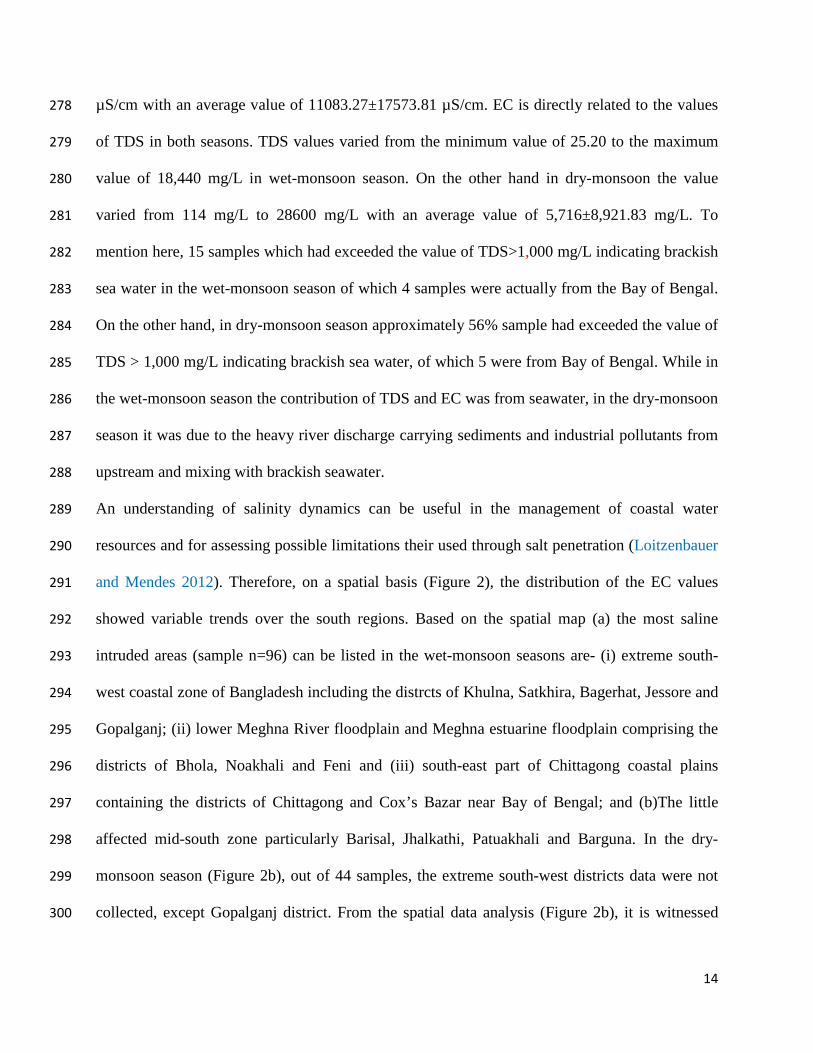
(Loitzenbauer and Mendes, 2012). EC values during wet-monsoon and dry-monsoon range from 276

65.90 to 34,800 µS/cm with an average value of 2,168.59±5,753.56 µS/cm and 228 to 57,300 277

14

µS/cm with an average value of 11083.27±17573.81 µS/cm. EC is directly related to the values 278

of TDS in both seasons. TDS values varied from the minimum value of 25.20 to the maximum 279

value of 18,440 mg/L in wet-monsoon season. On the other hand in dry-monsoon the value 280

varied from 114 mg/L to 28600 mg/L with an average value of 5,716±8,921.83 mg/L. To 281

mention here, 15 samples which had exceeded the value of TDS>1,000 mg/L indicating brackish 282

sea water in the wet-monsoon season of which 4 samples were actually from the Bay of Bengal. 283

On the other hand, in dry-monsoon season approximately 56% sample had exceeded the value of 284

TDS > 1,000 mg/L indicating brackish sea water, of which 5 were from Bay of Bengal. While in 285

the wet-monsoon season the contribution of TDS and EC was from seawater, in the dry-monsoon 286

season it was due to the heavy river discharge carrying sediments and industrial pollutants from 287

upstream and mixing with brackish seawater. 288

An understanding of salinity dynamics can be useful in the management of coastal water 289

resources and for assessing possible limitations their used through salt penetration (Loitzenbauer 290

and Mendes 2012). Therefore, on a spatial basis (Figure 2), the distribution of the EC values 291

showed variable trends over the south regions. Based on the spatial map (a) the most saline 292

intruded areas (sample n=96) can be listed in the wet-monsoon seasons are- (i) extreme south-293

west coastal zone of Bangladesh including the distrcts of Khulna, Satkhira, Bagerhat, Jessore and 294

Gopalganj; (ii) lower Meghna River floodplain and Meghna estuarine floodplain comprising the 295

districts of Bhola, Noakhali and Feni and (iii) south-east part of Chittagong coastal plains 296

containing the districts of Chittagong and Cox’s Bazar near Bay of Bengal; and (b)The little 297

affected mid-south zone particularly Barisal, Jhalkathi, Patuakhali and Barguna. In the dry-298

monsoon season (Figure 2b), out of 44 samples, the extreme south-west districts data were not 299

collected, except Gopalganj district. From the spatial data analysis (Figure 2b), it is witnessed 300

15

that in the dry season the district was affected by salinity. The above mentioned lower Meghna 301

River floodplain and Meghna estuarine floodplain comprising the districts of Bhola, Noakhali 302

and Feni and South-east part of Chittagong coastal plains containing the districts of Chittagong 303

and Cox’s Bazar near Bay of Bengal showed higher salinity concentration than that was in the 304

wet-monsoon season. Even mid-south zone particularly Barisal, Jhalkathi, Patuakhali, Pirojpur 305

and Barguna have been found to be affected. 306

In principle, salinity can refer to any inorganic ions, while in practise it is mostly the result of the 307

following major ions: Na+, Ca2+, Mg2+, K+, Cl−, SO42−, CO3

2− , and HCO3− (Williams 1987). 308

River water of the study area was clearly dominated by Na+, Mg2+, Ca2+, Cl−, HCO3−, and 309

SO42−during both of the seasons. During wet-monsoon and dry-monsoon seasons approximately 310

68.63% and 82.9% of the total cations and anions contributing to salinity were from Cl− which is 311

prevalent from the pie chart analysis (Figure 3a-b). In the wet-monsoon season the orders of 312

salinity contributing anions and cations were in the order of Cl−>HCO3−> SO4

2−>Na+ > 313

Ca2+>Mg2+>CO32¯. In the dry- monsoon season the order was Cl−>Na+> SO4

2−>HCO3−>Ca2+> 314

K+>Mg2+>CO32−. Increased load of Cl−, Na+, SO4

2−, HCO3− in the dry-monsoon season may 315

depict the opposite view due to landward movement of seawater. With respect to TDS and EC 316

samples of wet-monsoon and dry-monsoon seasons had shown the abundance of the major ions 317

is in the following order: Na+> Ca2+> K+> Mg2+ and Cl−> SO42−> HCO3

−> NO3−> CO3

2−. The 318

severe anions and cations variation in the dry-monsoon season may be attributed to the reduction 319

of flows of freshwater through increased upstream abstraction and increases of intrusion from 320

sea to land. The greater the penetration of marine influence into the land, the lower is the 321

availability of freshwater, which becomes brackish through its mixture with saline waters 322

(Loitzenbauer and Mendes 2012). 323

16

It was observed from the sample analysis that mean value of NO3− varied with the season from 324

0.1 mg/L to 43 mg/L in wet-monsoon season and 0.09 mg/L to 6.95 mg/L in the dry monsoon 325

season. The reason for seasonal nitrogen variation may be attributed to the nonpoint run off of 326

agricultural input of fertilizers and pesticides. Rainfall-runoff increased NO3− load in the wet-327

monsoon season while in dry-monsoon the load was reduced. Variation of PO43− remained 328

identical in both seasons with an average value of 0.31±0.80 mg/L. In addition, fluoride, iodide 329

and bromide all three anions were found to be higher in wet-monsoon season. In the wet-330

monsoon season concentration of fluoride, iodide and bromide varied from minimum 0 mg/L to 331

3.51 mg/L, 0 to 20.35 mg/L and 0 to 12.66 mg/L, respectively. Moreover, in the dry-monsoon 332

season the values of fluoride, iodide and bromide varied from 0 to 2.43 mg/L, 0.02 to 3.55 mg/L 333

and 0 to 2.24 mg/L respectively. Likewise all other anions and cations concentration, there was 334

colossal deviation of Fe concentration in both seasons. Concentration of Fe varied from a 335

minimum value of 0.05 to maximum value of 52.3 in the wet-monsoon season. While in the dry 336

monsoon season the minimum value started at 0.02 mg/L to maximum value of 37.60 mg/L. 337

Correspondingly B and Mn concentration in the wet-monsoon season accounted for 0.28 mg/L 338

and 0.14 mg/L on an average, whereas in dry-monsoon season the values accounted for 0.51 339

mg/L and 0.70 mg/L, respectively. The rise in the metal concentration might be related to the 340

upstream sediment carrying the metals rising in the dry-monsoon. 341

To find out more on the interrelations among various anions and cations in respect to EC and 342

TDS, Pearson's correlation matrix was prepared for wet-monsoon season (Table 2) and dry-343

monsoon season (Table 3) taking into account of 13 hydrochemical variables including pH, EC, 344

TDS, Ca2+, Mg2+, Na+, K+, Cl−, CO3²−, HCO3−, NO3

−, SO42− and PO4

3−. According to Table 2, 345

statistically positive significant correlations were found between EC and TDS (r = 0.99). 346

17

Subsequently, TDS and EC showed strong significant correlation with K+(r= 96 and 97), Cl¯ 347

(r=99 and 99) and SO42¯ (r=95 and 96). Other strong correlation that were observed from the 348

matrix were K+ and Cl− (r=97) and K+ and SO42−(r= 0.96). Moreover, Mg2+, Ca2+, Na+, K+, Cl−, 349

CO3²− and SO42− all had shown a weak but significant correlation with EC and TDS. The results 350

may be attributed to the high salinity nature of coastal river water along with precipitation and 351

heavy discharge from upstream. In addition, pH was negatively correlated with Mg2+ and CO32− 352

anion. Likewise in the dry-monsoon season statistically positive significant correlations were 353

found between EC and TDS (r = 0.99) (Table 3). Successively, TDS and EC showed strong 354

significant correlation with Cl¯ (r=99) and K+ (r= 96 and 97). Mg2+, Ca2+, Na+, K+, Cl−, HCO3− 355

and SO42− all showed weak but significant correlation with EC and TDS. This was further 356

confirmed by Principle component analysis (PCA) (Table 4, Figure 4a-b). 357

PCA is a multivariate statistical method complementary to classical approaches of 358

hydrogeochemical research (Morell et al. 1996). PCA provides a quick visualization and shows 359

correlation among different water quality variables. PCA was applied by considering 13 360

variables containing pH, EC, TDS, Ca2+, Mg2+, Na+, K+, Cl−, CO3²−, HCO3−, NO3

−, SO42− and 361

PO43−. For wet monsoon season PCA on the combined datasets provided three factors with 362

eigen value>1 that can explain approximately 67.84% of the variability of the data (PC 1 363

variance of 42.11% and PC 2 variance of 15.37%) (Table 4). From the biplot analysis of PCA, 364

when two variables are far from the centre and close to each other, then the variables are said to 365

be significantly and positively correlated (r=1). In the wet-monsoon season coefficients of PC1 366

which were related to the salinity of the river water closely related to EC, TDS, Cl−, K+ and 367

SO42− (Figure 4a). PC 2 which might be related to the inorganic carbon content of the river 368

HCO3− and CO3

2− in a weak relation to Na+, Mg2+ and Ca2+. On the other hand, for dry- 369

18

monsoon season PCA on the combined datasets provided four factors with eigenvalue >1 that 370

could explain approximately 54.97% of the variability of the data (PC 1 variance of 38.40% and 371

PC 2 variance of 16.58%) (Table 4). From the biplot analysis of PCA in dry-monsoon season, 372

coefficients of PC1 was related to the salinity of the river water unlike wet-monsoon season. The 373

closely related variables of EC and TDS to Cl− and K+ are shown in Figure 4(b). However, unlike 374

PCA of wet-monsoon season it was challenging to find out the second set of component (PC 2) 375

as there was not any strong relationship among the variables to support the assumptions. 376

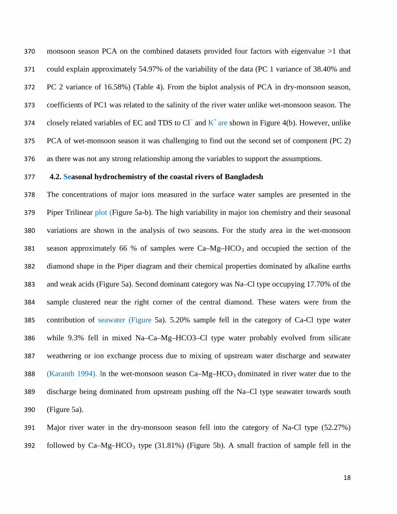
4.2. Seasonal hydrochemistry of the coastal rivers of Bangladesh 377

The concentrations of major ions measured in the surface water samples are presented in the 378

Piper Trilinear plot (Figure 5a-b). The high variability in major ion chemistry and their seasonal 379

variations are shown in the analysis of two seasons. For the study area in the wet-monsoon 380

season approximately 66 % of samples were Ca–Mg–HCO3 and occupied the section of the 381

diamond shape in the Piper diagram and their chemical properties dominated by alkaline earths 382

and weak acids (Figure 5a). Second dominant category was Na–Cl type occupying 17.70% of the 383

sample clustered near the right corner of the central diamond. These waters were from the 384

contribution of seawater (Figure 5a). 5.20% sample fell in the category of Ca-Cl type water 385

while 9.3% fell in mixed Na–Ca–Mg–HCO3–Cl type water probably evolved from silicate 386

weathering or ion exchange process due to mixing of upstream water discharge and seawater 387

(Karanth 1994). In the wet-monsoon season Ca–Mg–HCO3 dominated in river water due to the 388

discharge being dominated from upstream pushing off the Na–Cl type seawater towards south 389

(Figure 5a). 390

Major river water in the dry-monsoon season fell into the category of Na-Cl type (52.27%) 391

followed by Ca–Mg–HCO3 type (31.81%) (Figure 5b). A small fraction of sample fell in the 392

19

category of Ca-Cl and mixed type. In the dry-monsoon season Na–Cl type sea-water dominates 393

over Ca–Mg–HCO3 type due to limited river water discharge from upstream and pushing the 394

salinity front towards north. 395

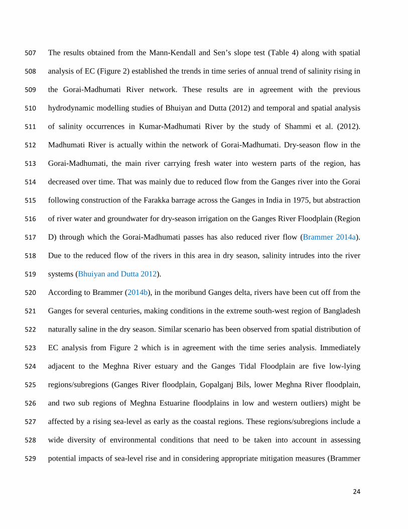
4.3. Analysis of molar ratio to identify seawater intrusion 396

Constant records of pre and dry-monsoon hydrochemistry are important to study the coastal river 397

water salinity and its fluctuation trends. Moreover ionic ratios reveal information about processes 398

in water bodies more visibly than concentrations (Siebert et al. 2014). In this paper Cl/Br molar 399

ratio, Na/Cl molar ratio, K/Cl molar ratio, Mg/Ca molar ratio were used to distinguish seawater 400

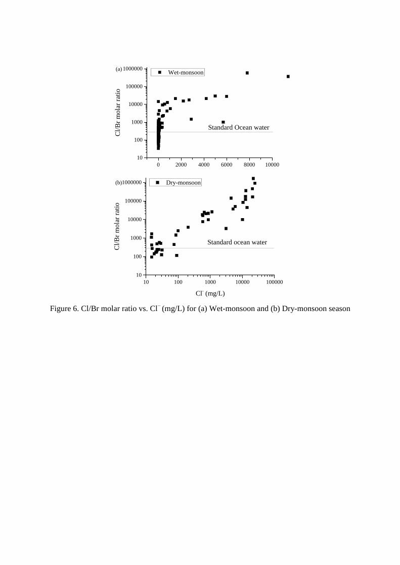
intrusion. The Cl/Br molar ratio can be obtained by multiplying mass ratio by 2.254. The 401

variation in Cl/Br molar ratio in sea water is about 290±4 (Katz et al. 2011). A Cl/Br molar ratio 402

vs. Cl (mg/L) depicts the sample affected by seawater intrusion (Figure 6). Approximately 77% 403

sample in the dry-monsoon had crossed the Cl/Br molar ratio of sea water at 290 compared to the 404

wet-monsoon season affected by approximately 34% sample. From Figure 6 it is clear that 405

seawater was affecting the salinity trend of the river water more in dry-monsoon compared to the 406

wet-monsoon season. In the wet-monsoon season Na/Cl molar ratio varied from minimum value 407

of 0 to 39.42 with average value 1.28±4.09. On the other hand, dry-monsoon season it varied 408

from 0.01 to 3.83 with average value 0.76±0.75 (Table 5). Approximately 23% sample collected 409

in the wet-monsoon season and 40% sample collected in the dry-monsoon had Na/Cl ratio above 410

0.86 indicating seawater intrusions. The spatial distribution of Na/Cl ratio for both seasons is 411

depicted in Figures 7a-b by utilizing ordinary kriging (OK) method. It was clear from the spatial 412

distribution map that dry-monsoon season was highly saline affected in the common sampling 413

points in the sapling point areas. Moreover, from Br/Cl molar ratio, it was found that in the wet-414

monsoon season approximately 62% and in dry-monsoon approximately 90% sample had molar 415

20

ratio above >0.0015 (Table 5). In wet-monsoon season Mg/Ca molar ratio varied from minimum 416

value of 0.001 to 32.36 with an average value of 1.69 while in dry-monsoon season it varied 417

from 0.08 to 93.66 with an average value of 4.37. However, only 3 samples in wet-monsoon and 418

dry-monsoon seasons had shown Mg/Ca molar ratio >5. Therefore, from the above data analysis 419

it was perceived that the existence of seasonal variation in anions and cations over time in 420

respect to salinity occurrences due to seawater intrusion and low upstream water flow in the river. 421

422

4.4. Fluctuation of salinity trends in the coastal rivers of Bangladesh 423

Understanding the dynamics of salinity gives a useful instrument for environmental monitoring 424

in an estuarine zone (Loitzenbauer and Mendes 2012). Therefore, it is also very important to 425

understand annual trends of time-series data of salinity in the rivers. In this context, trends of 426

salinity variation are very important for the surface water quality of coastal Bangladesh which 427

was investigated by traditional hydrochemistry parameter electrical conductivity (EC) data of 428

different rivers using Mann–Kendall and Sen’s slope test statistics. The results obtained from the 429

Mann-Kendall test was used to establish the trends in time series of annual salinity trends in the 430

13 river stations belonging to the Gorai River network of south-west zone of Bangladesh whether 431

they were increasing, decreasing, stable or trendless over time. Sen’s slope test was also used to 432

identify the significant level of increasing or decreasing trend and a comparison of their value is 433

presented in Table 6. 434

435

Findings from Mann-Kendall test also obtained the annual trend of salinity rising in the 436

Madhumati River significantly (confidence factor 98.9%). Other rivers which showed increasing 437

trend of salinity are Rupsa River, Khulna; Kakshiali River, Satkhira; Morichan River, Satkhira; 438

21

and Shibsha River, Khulna with confidence factor 96.9− 99.9%. The result is also in agreement 439

with the spatial analysis of EC (Figure 2). Similar result of increasing salinity trend has been 440

found in the MAKESENS tool kit for Madhumati River at 0.1 level of significance; Kakshiali 441

River, Satkhira at 0.001 level of significance; Morichan River, Satkhira at 0.01 level of 442

significance and Shibsha river, Khulna at 0.05 level of significance (Table 6). However, one 443

river Panguchi River, Bagerhat found to be decreasing in salinity trend in both tool kit analyses 444

at 0.1 level of significance in MAKESENS and 98.9% confidence factor in GSI toolkit analysis. 445

Two rivers Pasur River, Bagerhat and Vadra River, Khulna showed “Probably increasing” trend 446

with confidence interval 91.1% and 94.6%, respectively in GSI tool kit analysis. Although 447

seasonal variations in the EC was found higher during trend analysis, overall annual analysis of 448

the salinity trend was found to be “stable” over time for Kapotaksha River, Satkhira. Moreover, 449

five rivers showed “no trend” in the analysis. The rivers are Daratana River, Bagerhat; Shailmari 450

River, Khulna; Betna River, Satkhira; Kazibachha River, Khulna and Shibsha Rivers, Khulna. 451

The causes of the variability in salinity trends in the above mentioned rivers are likely related to 452

the local hydrogeologic condition, tidal effects from the Bay of Bengal, local rainfall-runoff 453

condition, and climatic events. Besides these extreme western parts of rivers are actually parts of 454

the moribund Ganges Delta. 455

5. Discussions 456

It is evident from our result that there is a marked seasonal variation exists in the hydrochemistry 457

of coastal rivers in Bangladesh. There is a significant variation in anions and cations contributing 458

to the salinity variation may be associated to at the Ganges-Brahmaputra-Meghna (GBM) River 459

discharge as well as inland rainfall-runoff. Seasonal variation of anions and cations were 460

significantly marked from the results. It was particularly evident in the nitrate variation in the 461

22

surface water. In Bangladesh the rainfed aman rice cultivation is widespread along the coastal 462

areas (Shelley et al. 2016). It was apparent that wet-monsoon season NO3− indicated agricultural 463

source and fertilizers application of transplanted aman (t. aman) production. NO3− containing 464

fertilizer such as urea is applied 24 kg/3330m² in t. aman production (FAO 2017). Seeding time 465

of aman rice is between March and April and transplanted between July and August during wet-466

monsoon period. The crop is harvested from November through December (Shelley et al. 2016) 467

during the start of dry-monsoon period. 468

The up scaled monthly discharge of GBM river mouths produced for oceanographic 469

investigations exhibited a marked seasonal and inter annual variability (Papa et al. 2012). The 470

impact of Farakka Dam on the Lower Ganges River flow was calculated by comparing threshold 471

parameters for the pre-Farakka period (from 1934 to 1974) and the post-Farakka period (1975–472

2005). In a normal hydrological cycle, rivers in Bangladesh suffer from low flow conditions 473

when there is no appreciable rainfall runoff. The discharge of river is 80,684 m3/s during the 474

flood or wet-monsoon season while during the dry-monsoon season when the inflow is very low, 475

discharge can be as low as 6041 m3/s (Ahmed and Alam 1999). The results demonstrate that due 476

to water diversion by the Farakka Dam, various threshold parameters, including the monthly 477

mean of the dry season (December–May) and yearly minimum flows have been altered 478

significantly. The ecological consequences of such hydrologic alterations include the increase of 479

salinity in the southwest coastal region of Bangladesh (Gain and Giupponi 2014). 480

This further validates the seasonal shifting of Na-Cl dominated salinity front and molar ratio of 481

Na/Cl, Br/Cl Mg/Ca. Seawater has distinct ionic and isotopic ratios such as Na/Cl=0.86, 482

Br/Cl=0.0015, Mg/Ca=5.2 (Vengosh et al. 1999; Vengosh and Rosenthal 1994). A Na/Cl ratio of 483

0.86 was thought to indicate sea water intrusion (Bear et al. 1999). The Na/Cl molar ratio could 484

23

reach unity due to the mixing of seawater and freshwater, which had a Na/Cl ratio greater than 485

unity (Vengosh and Rosenthal 1994). Mg/Ca molar ratio greater than 5 is a direct indicator of 486

seawater intrusion (Vengosh and Ben-Zvi 1994). Significant variation was observed during wet-487

monsoon season and dry-monsoon season from the molar ratio study of Na/Cl, Br/Cl Mg/Ca 488

indicating seawater intrusion. Chloride and bromide ions have been used to differentiate among 489

various sources of anthropogenic and naturally occurring contaminants in groundwater (Katz et 490

al. 2011). The elements in the estuaries are typically assessed by making plots of their dissolved 491

concentrations vs. salinity. Several elements are removed from the dissolved phase whereas 492

some elements are also released from the suspended particles (Samanta and Dalai 2016). In the 493

present study significant changes in the values of Cl/Br molar ratio, Na/Cl molar ratio, K/Cl 494

molar ratio, Mg/Ca molar ratio in the dry-monsoon compared to the wet-monsoon season 495

indicate saline water intrusion in the coastal rivers. To support the scenario a similar seasonal 496

changes in δ18O from Hooghly Estuary (India) was observed. The study had identified low 497

salinity and depleted δ18O during monsoon was consistent with increased river discharge as well 498

as high rainfall. This was driven by composition of the freshwater source which was dominated 499

by rainwater during monsoon and rivers during non-monsoon months (Ghosh et al. 2013). 500

Furthermore, presence of seawater was found maximum (31–37%) during February till July and 501

lowest (less than or equal to 6%) from September till November. A temporal offset between 502

Ganges River discharge farther upstream at Farakka and salinity variation at the Hooghly 503

Estuary was observed (Ghosh et al. 2013). Similar situation has been observed from the seasonal 504

changes in hydrochemistry of anions, cations, Na-Cl dominated salinity front and molar ratio 505

study of different anions and cations. 506

24

The results obtained from the Mann-Kendall and Sen’s slope test (Table 4) along with spatial 507

analysis of EC (Figure 2) established the trends in time series of annual trend of salinity rising in 508

the Gorai-Madhumati River network. These results are in agreement with the previous 509

hydrodynamic modelling studies of Bhuiyan and Dutta (2012) and temporal and spatial analysis 510

of salinity occurrences in Kumar-Madhumati River by the study of Shammi et al. (2012). 511

Madhumati River is actually within the network of Gorai-Madhumati. Dry-season flow in the 512

Gorai-Madhumati, the main river carrying fresh water into western parts of the region, has 513

decreased over time. That was mainly due to reduced flow from the Ganges river into the Gorai 514

following construction of the Farakka barrage across the Ganges in India in 1975, but abstraction 515

of river water and groundwater for dry-season irrigation on the Ganges River Floodplain (Region 516

D) through which the Gorai-Madhumati passes has also reduced river flow (Brammer 2014a). 517

Due to the reduced flow of the rivers in this area in dry season, salinity intrudes into the river 518

systems (Bhuiyan and Dutta 2012). 519

According to Brammer (2014b), in the moribund Ganges delta, rivers have been cut off from the 520

Ganges for several centuries, making conditions in the extreme south-west region of Bangladesh 521

naturally saline in the dry season. Similar scenario has been observed from spatial distribution of 522

EC analysis from Figure 2 which is in agreement with the time series analysis. Immediately 523

adjacent to the Meghna River estuary and the Ganges Tidal Floodplain are five low-lying 524

regions/subregions (Ganges River floodplain, Gopalganj Bils, lower Meghna River floodplain, 525

and two sub regions of Meghna Estuarine floodplains in low and western outliers) might be 526

affected by a rising sea-level as early as the coastal regions. These regions/subregions include a 527

wide diversity of environmental conditions that need to be taken into account in assessing 528

potential impacts of sea-level rise and in considering appropriate mitigation measures (Brammer 529

25

2014b). A salinity flux model integrated with an existing hydrodynamic model was applied in 530

order to simulate flood and salinity in the complex waterways in the coastal zone of Gorai river 531

basin with sea level rise (SLR) scenario (Bhuiyan and Dutta 2012). The results of salinity model 532

obtained had indicated the risk and changes in salinity due to sea level rise with increased river 533

salinity as well as the salinity intrusion length in the river. Sea level rise of 59 cm produced a 534

change of 0.9 ppt at a distance of 80 km upstream of river mouth, corresponding to a climatic 535

effect of 1.5 ppt per meter SLR (Bhuiyan and Dutta 2012). The SLR depends not only on 536

changes in the mass and volume of sea water but also on other factors, such as local subsidence, 537

river discharge, sediment and the effects of vegetation (Lee 2013). Moreover, the SLR trend 538

obtained from ensemble empirical mode decomposition (EEMD) was 4.46 mm/yr over April 539

1990 to March 2009, which was larger than the recent altimetry-based global rate of 3.360.4 540

mm/yr over the period from 1993 to 2007 (Lee 2013). It is, therefore, important to determine the 541

impacts of SLR on salinity to devise suitable adaptation and mitigation measures and reduce 542

impacts of salinity intrusion in coastal cities (Bhuiyan and Dutta 2012). 543

The progressive inland movement of the dry-season salt-water limit in south-western rivers has 544

had adverse impacts on soil salinity, crop production and availability of potable domestic water 545

supplies in affected areas (Brammer 2014b). Increased salinity possesses a risk of secondary soil 546

salinization. Secondary soil salinization occurs when surface soil salinity has increased from 547

non-saline to a saline level as a consequence of irrigation or other agricultural practices (Peck 548

and Hatton 2003). The seasonal variation of using drinking water sources in the study area is 549

influenced by the monsoonal precipitation and the success of tube well installation factors 550

(Sarkar and Vogt 2015). Increased salinity of drinking water is likely to have a range of health 551

effects, including increased hypertension rates. Large numbers of pregnant women in the coastal 552

26

areas are being diagnosed with pre-eclampsia, eclampsia, and hyper tension (Khan et al. 2008). 553

The main drinking water sources used in the study area are the tube well, with an average depth 554

of 200 m, and pond, with or without the adjacent filtration facility known as PSF (pond sand 555

filter) (Sarkar and Vogt 2015). 556

Nevertheless, the coastal area of the country is known as one of the highly productive areas of 557

the world (Afroz and Alam 2013). With increasing levels of salinity in the land and freshwater 558

resources, the brackish water aquaculture flourished rapidly on agricultural land. The change in 559

land-use from agriculture to brackish water shrimp aquaculture has further increased the soil and 560

water salinization across the landscape (Shameem et al. 2014). Salinity increases may affect 561

survival of some mangroves and wetland plants, especially in dry season (Suen and Lai 2013). 562

Integrated Coastal Zone Management (ICZM) involves an integrated planning process to address 563

the complex management issues in the coastal area of Bangladesh (Afroz and Alam 2013). It is a 564

blueprint for sustainable coastal development (Afroz and Alam 2013) which is made up of three 565

broad categories of integration: (i) policy integration, (ii) functional integration and (iii) system 566

integration (Thia-Eng 1993). Despite increasing recognition of the need for ICZM strategies, the 567

initiation of the Coastal Zone Policy and ICZM has not contributed any significant improvement 568

in the coastal areas (Rahman and Rahman 2015) of Bangladesh. Introduction of advanced coastal 569

protection models must incorporate the complexity of natural environmental variation, including 570

the influence of both the biotic and abiotic ecosystem (Spalding et al. 2014). A model should be 571

synthesized to optimize conjunctive uses of the water in the affected area based on two questions: 572

“Which water resources to use?” and “When to use which water source?” for the best 573

management of water resources. Introducing water resources information system aims to build a 574

data-bank of water resources and factors influencing their management (Loitzenbauer and 575

27

Mendes 2012). This data bank will provide information of existing and potential water resources 576

for optimum uses of water without compromising the quality of water. 577

The salinity balance of each coastal river basins, including that of the Ganges, Gorai-Madhumati, 578

Meghna, Karnafuli and other river networks should form part of this data-bank, together with the 579

results from modeling the salinity distribution which requires regular trend analysis to combat 580

not only salinity intrusion in the coastal areas but may help to combat other problems including, 581

agricultural-non-point nutrient pollution, hypoxia, eutrophication, sewage pollution, industrial 582

pollution and other problems. It is important to understand and communicate the economic, 583

environmental and social costs of river salinization in order to guide management and restoration 584

efforts. Impacts need to be anticipated and mitigated, and future scenarios of climate change and 585

increasing water demand have to be integrated into the ecological impact assessment (Canedo-586

Arguelles et al. 2013). Consequently, for sustaining the ecosystem integrity of coastal rivers and 587

estuaries, it is very important to restore and maintain minimum environmental flow assessment 588

(EFA) of the major shared rivers with India. In the “Bangladesh: National Programme of Action 589

for Protection of the Coastal and Marine Environment from Land-Based Activities” 590

(DoE/MOEF/GOB 2006) strategy 5 clearly stated assessment of environmental flow requirement 591

and salinity intrusion in the Integrated Coastal Zone Management Plan (ICZMP). In this regard a 592

complete regional water management plan for the Ganges-Brahmaputra-Meghna catchment area 593

is needed along with minimum EFA in the lower estuarine and coastal regions of Bangladesh to 594

maintain ecological integrity of the region. However, to-date, India has not prepared any EFA of 595

the joint rivers to support such a plan or to share hydrological data with Bangladesh (Brammer 596

2004). Moreover, this plan should be carried out with other countries of shared river including 597

Nepal and China. 598

28

6. Conclusions and remarks 599

Trend analysis is one of the most important issues in any regional hydrological variables taking 600

into account the spatial and temporal variable and providing result for present conditions and 601

future scenario from past data analysis. In this context, spatial records of wet- and dry-monsoon 602

salinity levels in the southern coastal rivers and estuary are important to study the level of 603

salinity fluctuation trends of coastal areas of Bangladesh. The differences between wet- and dry-604

monsoon salinity levels, represents the combined effect of salinity scenario in the southern 605

region. The results obtained from the historical trend analysis by Mann-Kendall test and Sen’s 606

slope was used to establish the trends in time series. In this framework, the conclusions and 607

remarks, which can be significant from this study, are: 608

a) EC and TDS is the principal component of salinity along with K+, Cl− and SO42− as observed 609

from both wet-monsoon and dry-monsoon seasonal analysis in relation to the other anions 610

and cations. Moreover, on a spatial basis the distribution of the EC values showed variable 611

trends over the south regions. The most saline intruded areas in the wet-monsoon season is 612

(i) Extreme south-west coastal zone of Bangladesh comprising the distrcts of Khulna, 613

Satkhira, Bagerhat, Jessore and Gopalganj; 614

(ii) Lower Meghna River floodplain and Meghna estuarine floodplain comprising the 615

districts of Bhola, Noakhali and Feni; 616

(iii) South-east part of Chittagong coastal plains containing the districts of Chittagong and 617

Cox’s Bazar near Bay of Bengal; 618

(iv) The little affected mid-south zone particularly Barisal, Jhalkathi, Patuakhali and 619

Barguna which are also being affected in the dry-monsoon season 620

621

29

b) From the hydrochemistry analysis of piper diagram in the wet-monsoon season 622

approximately 66% of samples were Ca–Mg–HCO3 type and second prevailing category was 623

Na–Cl type subjugating 17.70% samples. In the dry-monsoon season foremost water type fell 624

into the category of Na-Cl type (52.27%) followed by Ca–Mg–HCO3 type (31.81%). 625

c) Seawater intrusion was also confirmed by calculated ionic ratios. It was found from Cl/Br 626

molar ratio vs. Cl− that about 42.7% of the collected sample water was affected by salinity in 627

wet-monsoon season compared to the 27% collected in dry-monsoon. Moreover roughly 628

33.33% sample collected in the wet-monsoon season and 38.63% sample collected in the 629

dry-monsoon had Na/Cl ratio above 0.86 indicating sea-water-intrusion. 630

d) From Mann-Kendall and Sen’s slope test analysis it was prevalent that among the 13 river 631

time series analysis of salinity trend, four rivers had shown significantly increasing trend of 632

salinity in the extreme south-west zone of Bangladesh. This also signify the future work 633

analysis of other major rivers affected by salinity particularly in other major rivers 634

particularly in Meghna river estuary and eastern Chittagong coastal plains zones. These 635

outcomes deliver the following perceptions for future mechanisms. 636

637

On equilibrium, the result of this study proves the extent of seawater intrusion in the coastal 638

rivers by using an interdisciplinary approach. Moreover, the hydrochemical data in conjunction 639

with the remote sensing and GIS and statistical methods identified the spatial extent of salinity 640

occurrences in a seasonal basis. With the application of Mann-Kendall and Sen’s slope this 641

research further assessed salinity rising trend in south-west coastal zones of Bangladesh. In order 642

to predict future trends in other rivers, the same method can be utilized to predict future trends of 643

seawater intrusion. This method can be further applied to study other environmental processes to 644

30

assess. The results of this study can also provide important information and a priori assessment 645

to water resource managers, engineers, practitioners and policy makers and environmental 646

scientists of the country to implement structures for the management of important water 647

resources. This study could further help to comprehend seasonal trends in the hydrochemistry 648

and water quality of the coastal and estuarine rivers, and help policy makers to obligate some 649

important implications for the future initiatives taken for the management of land, water, fishery, 650

agriculture and environment of coastal rivers and estuaries of Bangladesh. 651

652

Conflicts of Interest 653

All authors have read the manuscript and declared no conflict of interests. All authors discussed 654

the results and implications and commented on the manuscript at all stages. 655

656

Acknowledgements 657

This work has been supported by the project entitled “Establishment of monitoring network and 658

mathematical model study to assess salinity intrusion in groundwater in the coastal area of 659

Bangladesh due to climate change” implemented by Bangladesh Water Development Board and 660

sponsored by Bangladesh Climate Change Trust Fund, Ministry of Environment and Forest. 661

662

References 663

Afroz T, Alam S (2013) Sustainable shrimp farming in Bangladesh: A quest for an Integrated 664

Coastal Zone Management. Ocean Coast Manage 71: 275-283 665

Ahamed AU, Alam M (1999) Development of Climate Change Scenarios with General 666

Circulation Models. in: Saleemul Huq, Z. Karim, M. Asaduzzaman, and F. Mahtab (eds.) 667

31

Vulnerability and Adaptation to Climate Change for Bangladesh.Kluwer Academic 668

Publishers, Dordrecht, the Netherlands. pp. 13-20. 669

Aziz JJ, Ling M, Rifai HS, Newell CJ, Gonzales JR (2003) MAROS: A decision support system 670

for optimizing monitoring plans. Ground Water 41(3): 355-367 671

Bahar MM, Reza MS (2010) Hydrochemical characteristics and quality assessment of shallow 672

groundwater in a coastal area of Southwest Bangladesh. Environ Earth Sci 61(5): 1065-673

1073 674

Bear J (1999) Seawater intrusion in coastal aquifers: concepts, methods and practices. Boston. 675

Mass: Kluwer Academic. 676

Bhuiyan MJAN, Dutta D (2012) Assessing impacts of sea level rise on river salinity in the Gorai 677

river network, Bangladesh. Estuar Coast Shelf Sci 96: 219-227 678

Brammer H (2004) Can Bangladesh be Protected from Floods? University Press Ltd, Dhaka. 679

Brammer H (2014a) Climate Change, Sea-level Rise and Development in Bangladesh, 680

University Press Ltd, Dhaka. 681

Brammer H (2014b) Bangladesh’s dynamic coastal regions and sea-level rise. Climate Risk 682

Manage 1: 51-62 683

Canedo-Arguelles M, Kefford BJ, Piscart C, Prat N, Schafer RB, Schulz CJ (2013) Salinisation 684

of rivers: an urgent ecological issue. Environ Pollut 173: 157-67 685

DoE/MOEF/GOB (2006)Bangladesh, national programme of action for protection of the coastal 686

and marine environment from land-based activities. Department of Environment, 687

Ministry of Environment and Forests, Government of the People's Republic of 688

Bangladesh, Dhaka. 689

32

Da Lio C, Carol E, Kruse E, Teatini P, Tosi L (2015) Saltwater contamination in the man aged 690

low-lying farmland of the Venice coast, Italy: An assessment of vulnerability. Sci Total 691

Environ 533: 356-69 692

FAO (1985) FAO report on tidal area study. Fisheries resources survey system. FAO/UNDP-693

BGD/79/015.http://www.fao.org/docrep/field/003/ac352e/AC352E00.htm#TOC. 694

Accessed on 15th March 2016 695

FAO (2017) Applying flexible cropping schedules for rice (t. aman) production in 696

Bangladesh. http://teca.fao.org/read/6853. Accessed 30thJanuary 2017 697

Ghabayen SMS, McKee M, Kemblowski M (2006) Ionic and isotopic ratios for identification of 698

salinity sources and missing data in the Gaza aquifer. J Hydrol 318(1-4): 360-373 699

Gain A, Giupponi C (2014) Impact of the Farakka Dam on thresholds of the hydrologic flow 700

regime in the lower Ganges River basin (Bangladesh). Water6(8): 2501-2518 701

Ghosh P, Chakrabarti R, Bhattacharya SK (2013) Short- and long-term temporal variations in 702

salinity and the oxygen, carbon and hydrogen isotopic compositions of the Hooghly 703

Estuary water, India. Chem Geol 335: 118-127 704

Halim MA, Majumder RK, Nessa SA, Hiroshiro Y, Sasaki K, Saha BB, Saepuloh A, Jinno K 705

(2010) Evaluation of processes controlling the geochemical constituents in deep 706

groundwater in Bangladesh: spatial variability on arsenic and boron enrichment. J Hazard 707

Mater 180(1-3): 50-62 708

Islam MA, Zahid A, Rahman MM, Rahman MS, Islam MJ, Akter Y, Shammi M, Bodrud-Doza 709

M, Roy B (2016) Investigation of Groundwater Quality and Its Suitability for Drinking 710

and Agricultural Use in the South Central Part of the Coastal Region in Bangladesh. 711

Expo Health. Doi: 10.1007/s12403-016-0220-z 712

33

Jiang Y, Guo H, Jia Y, Cao Y, Hu C (2015) Principal component analysis and hierarchical 713

cluster analyses of arsenic groundwater geochemistry in the Hetao basin, Inner Mongolia. 714

Chem Erde Geochem 75(2): 197-205 715

Karanth KR (1994) Groundwater Assessment Development and Management, Tata McGraw-716

Hill Publishing Company Limited, New Delhi, (third reprint). 717

Katz BG, Eberts SM, Kauffman LJ (2011) Using Cl/Br ratios and other indicators to assess 718

potential impacts on groundwater quality from septic systems: A review and examples 719

from principal aquifers in the United States. J Hydrol 397(3-4): 151-166 720

Kendall MG (1975) Rank correlation methods. Griffin, London 721

Khan A, Mojumder SK, Kovats S, Vineis P (2008) Saline contamination of drinking water in 722

Bangladesh. Lancet 371(9610): 385 723

Kisi O, Ay M (2014) Comparison of Mann–Kendall and innovative trend method for water 724

quality parameters of the Kizilirmak River, Turkey. J Hydrol 513: 362-375 725

Lee HS (2013) Estimation of extreme sea levels along the Bangladesh coast due to storm surge 726

and sea level rise using EEMD and EVA. J Geophys Res: Oceans 118(9): 4273-4285 727

Loitzenbauer E, Mendes CAB (2012) Salinity dynamics as a tool for water resources 728

management in coastal zones: An application in the Tramandaí River basin, southern 729

Brazil. Ocean Coast Manage 55: 52-62 730

Mann HB (1945) Nonparametric tests against trend. Econometrica 13:245–259 731

MoWR (2005)Coastal Zone Policy (CZPo), Ministry of Water Resources (MoWR) 732

Niazi F, Mofid H, Modares FN (2014) Trend analysis of temporal changes of discharge and 733

water quality parameters of Ajichay River in four recent decades. Water Qual Exp Health 734

6(1-2): 89-95 735

34

Otache M, Bakir M, Zhijia L (2008) Analysis of stochastic characteristics of the Benue River 736

flow process. Chin J Oceanol Limn 26(2): 142-151 737

Papa F, Bala SK, Pandey RK, Durand F, Gopalakrishna VV, Rahman A, Rossow WB (2012) 738

Ganga-Brahmaputra river discharge from Jason-2 radar altimetry: An update to the long-739

term satellite-derived estimates of continental freshwater forcing flux into the Bay of 740

Bengal. J Geophys Res: Oceans117: C11021 741

Peck AJ, Hatton T (2003) Salinity and the discharge of salts from catchments in Australia. J 742

Hydrol 272: 191-202. 743

Piper AM (1944) A graphic procedure in the geochemical interpretation of water analyses. Am 744

Geoph Union Trans 25: 914-923 745

Rahman AM, Rahman S (2015) Natural and traditional defense mechanisms to reduce climate 746

risks in coastal zones of Bangladesh. Weather Climate Extremes 7: 84-95 747

Salmi T, Maata A, Antilla P, Ruoho-Airola T, Amnell T (2002) Detecting trends of annual 748

values of atmospheric pollutants by the Mann–Kendall test and Sen’s slope estimates-the 749

Excel template application MAKESENS. Finnish Meteorological Institute, Helsinki, 750

Finland. 751

Samanta S, Dalai T (2016) Dissolved and particulate Barium in the Ganga (Hooghly) River 752

estuary, India: solute-particle interactions and the enhanced dissolved flux to the oceans. 753

Geochim Cosmochim Acta 195: 1-28 754

Sarkar R, Vogt J (2015) Drinking water vulnerability in rural coastal areas of Bangladesh during 755

and after natural extreme events. Int J Disaster Risk Reduct 14: 411-423 756

Sen PK (1968) Estimates of the regression coefficient based on Kendall’s tau. J Am Stat Assoc 757

63:1379–1389 758

35

Shahid S (2010) Trends in extreme rainfall events of Bangladesh. Theor Appl Climatol 104(3-4): 759

489-499 760

Shameem MIM, Momtaz S,Rauscher R (2014) Vulnerability of rural livelihoods to multiple 761

stressors: A case study from the southwest coastal region of Bangladesh. Ocean Coast 762

Manage 102: 79-87. 763

Shammi M, Bhuiya G, Ibne Kamal A, Rahman M, Rahman M, Uddin M (2012) Investigation of 764

Salinity Occurrences in Kumar-Madhumati River of Gopalganj District, Bangladesh. J 765

Nature Sci Sustainable Technol 6(4): 299-313 766

Shammi M, Karmakar B, Rahman M, Islam M, Rahman R, Uddin M (2016) Assessment of 767

salinity hazard of irrigation water quality in monsoon season of Batiaghata Upazila, 768

Khulna District, Bangladesh and adaptation strategies. Pollution 2: 183-197 769

Shelley I, Takahashi-Nosaka M, Kano-Nakata M, Haque M, Inukai Y (2016) Rice cultivation in 770

Bangladesh: present scenario, problems, and prospects. J Intl Cooper Agric Dev 14: 20-771

29 772

Siebert C, Möller P, Geyer S, Kraushaar S, Dulski P, Guttman J, Subah A, Rödiger T (2014) 773

Thermal waters in the Lower Yarmouk Gorge and their relation to surrounding aquifers. 774

Chem. Erde Geochem. 74(3): 425-441 775

Spalding MD, Ruffo S, Lacambra C, Meliane I, Hale LZ, Shepard CC, Beck MW (2014) The 776

role of ecosystems in coastal protection: Adapting to climate change and coastal hazards. 777

Ocean Coast Manage 90: 50-57 778

Suen J-P, Lai H-N (2013) A salinity projection model for determining impacts of climate change 779

on river ecosystems in Taiwan. J Hydrol 493: 124-131 780

36

Takeuchi K, Xu ZX, Ishidiaira H (2003) Monitoring trend step changes in precipitation in 781

Japanese precipitation. J Hydro 279:144–150 782

Trabelsi N, Triki I, Hentati I, Zairi M (2016) Aquifer vulnerability and seawater intrusion risk 783

using GALDIT, GQISWI and GIS: case of a coastal aquifer in Tunisia. Environ Earth Sci 784

75(8): 1-19 785

Thia-Eng C (1993) Essential elements of integrated coastal zone management.Ocean Coast 786

Manage 21: 81-108 787

Vengosh A, Heumann KG, Juraski S, Kasher R (1994) Boron isotope application for tracing 788

sources of contamination in groundwater. Environ Sci Technol 28 (11): 1968–1974 789

Vengosh A, Spivack AJ, Artzi Y, Ayalon A (1999) Geochemical and Boron, Strontium, and 790

Oxygen isotopic constraints on the origin of the salinity in groundwater from the 791

Mediterranean coast of Israel. Water Resour Res 35(6): 1877–1894 792

Vengosh A, Ben-Zvi A (1994) Formation of a salt plume in the coastal plain aquifer of Israel: the 793

Be’erToviyya region. J Hydrol 160: 21–52 794

Vengosh A, Rosenthal E (1994) Saline groundwater in Israel: Its bearing on the water crisis in 795

the country. J Hydrol 156: 389–430 796

Webster R, Oliver M (2001) Geostatistics for environmental scientists. John Wiley & Sons, Ltd, 797

Chichester, Sussex. 798

Werner AD, Bakker M, Post VEA, Vandenbohede A, Lu C, Ataie-Ashtiani B, Simmons CT, 799

Barry DA (2013) Seawater intrusion processes, investigation and management: Recent 800

advances and future challenges. Adv Water Resour 51: 3-26 801

Williams WD (1987) Salinization of Rivers and streams: an important environmental hazard. 802

Ambio 16: 181-185 803

37

Williams WD, Sherwood J (1994) Definition and measurement of salinity in salt lakes. Int J Salt 804

Lake Res 3(1): 53-63 805

806

Figure file

Figure 1

Figure 2

Figure 3

Figure 4

Figure 5

Figure 6

Figure 7

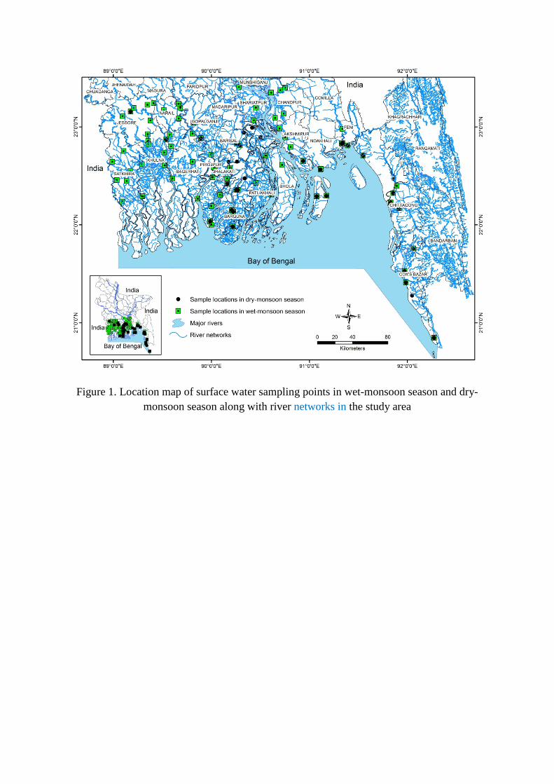
Figure 1. Location map of surface water sampling points in wet-monsoon season and dry-monsoon season along with river networks in the study area

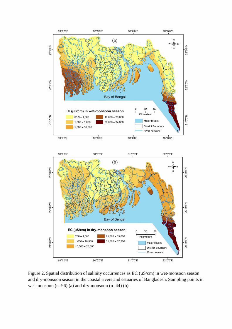
Figure 2. Spatial distribution of salinity occurrences as EC (µS/cm) in wet-monsoon season and dry-monsoon season in the coastal rivers and estuaries of Bangladesh. Sampling points in wet-monsoon (n=96) (a) and dry-monsoon (n=44) (b).

(a)

(b)

11.17%

9.82%

0.06%

68.63%

1.54%5.03%

1.12%2.62%

Ca2+

Mg2+

Na+

K+

Cl-

CO2-3

HCO-3

SO2-4

(a) Wet-monsoon season

5.6%

2.41%0.02%

82.9%

0.92%6.42%

0.75%0.98%

Ca2+

Mg2+

Na+

K+

Cl-

CO2-3

HCO-3

SO2-4

(b) Dry-monsoon season

Figure 3. Seasonal variation of anions and cations contributing to salinity in the major coastal rivers and estuarine water based on average data (a) variation in wet-monsoon season (b) variation in dry-monsoon season

Figure 4. PCA on the combined data sets of anions and cations with other important water parameters to understand seasonal variations of river water (a) Wet-monsoon season and (b) Dry-monsoon season

-2 0 2 4 6 8 10 12 14-4

-3

-2

-1

0

1

2

3

4

5

6-0.5 0.0 0.5 1.0 1.5 2.0 2.5 3.0 3.5 4.0

-0.6

-0.4

-0.2

0.0

0.2

0.4

0.6

0.8

1.0Pr

inci

pal C

ompo

nent

2

Principal Component 1

pH

K+Cl- SO2-

4

Ec TDSPO3-

4

Na+Mg2+Ca2+NO-

3

CO2-3

HCO-3

(a) Wet-monsoon season

0 2-3

-2

-1

0

1

2

3

4

-0.5 0.0 0.5 1.0

-0.6

-0.4

-0.2

0.0

0.2

0.4

0.6

0.8

Prin

cipa

l Com

pone

nt 2

Principal Component 1

NO-3

Na+SO2-4

Mg2+ Ca2+

EcTDSCl-K+

pHPO3-

4

CO2-3

HCO-3

(b) Dry-monsoon season

Figure 5. Piper diagram for major ion contents of surface waters of the study area to determine water types (a) wet-monsoon season and (b) dry-monsoon season. The surface waters are classified into three types; Type I: Ca–Mg–HCO3, Type II: Ca-Cl type, Type III: Na-Cl type, Type IV: Na–HCO3, Type V: mixed type Na–Ca–Mg–HCO3–Cl

0 2000 4000 6000 8000 1000010

100

1000

10000

100000

1000000

10 100 1000 10000 10000010

100

1000

10000

100000

1000000(b)

Wet-monsoon

Cl/B

r mol

ar ra

tioStandard Ocean water

(a)

Dry-monsoon

Cl/B

r mol

ar ra

tio

Cl- (mg/L)

Standard ocean water

Figure 6. Cl/Br molar ratio vs. Cl− (mg/L) for (a) Wet-monsoon and (b) Dry-monsoon season

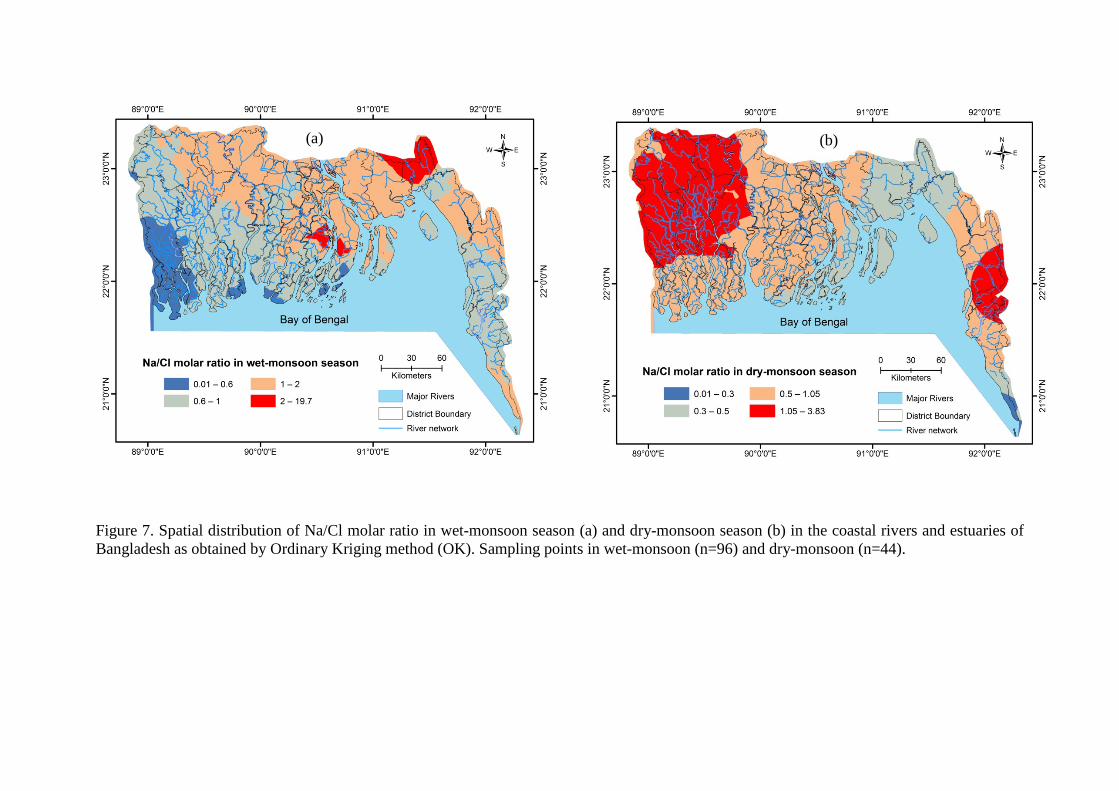
Figure 7. Spatial distribution of Na/Cl molar ratio in wet-monsoon season (a) and dry-monsoon season (b) in the coastal rivers and estuaries of Bangladesh as obtained by Ordinary Kriging method (OK). Sampling points in wet-monsoon (n=96) and dry-monsoon (n=44).

(b) (a)