A Variable-Step Interaction Algorithm for Multidisciplinary Collaborative Simulation Hongwei Wangb,c, Huachao Maoa and Heming Zhanga*

aNational CIMS Engineering Research Centre, Tsinghua University, Beijing, 100084, P.R.ChinabSchool of Engineering, University of Portsmouth, Portsmouth, PO1 3DJ, United KingdomcEngineering Design Centre, Engineering Department, University of Cambridge, Cambridge, CB2 1PZ, United Kingdom

Abstract. Multidisciplinary collaborative simulation is an important technique for the development of complex engineering systems such as aircrafts and automobiles. It emphasizes the synergic collaboration of multidisciplinary computational models, involving the exchange of simulation data generated in parallel at runtime from the numerical integration processes of these models. Current research on the interaction of models in multidisciplinary collaborative simulation is mainly focused on performing data exchange at fixed intervals, i.e. macro time steps, and using interpolation/extrapolation to find out values at the points in time when data are not available. However, the selection of an appropriate size for macro time tends to be complex and iterative. Firstly, it is mostly based on experience rather than the estimation of simulation errors by analyzing the numerical integration processes involved. Moreover, it is hardly possible to select a fixed step size suitable for all the stages of the simulation process. This paper presents a novel variable-step algorithm which is able to adjust the step size automatically at simulation runtime based on the evaluation of truncation errors. This algorithm not only avoids the instability and inaccuracy caused by a fixed large step but also speeds up the simulation by using a smaller step when a large one is not necessary. It is demonstrated in the numerical experiments that the variable-step algorithm can achieve improved simulation performance in terms of both speed and accuracy.

Keywords: product design, collaborative simulation, numerical integration, truncation error estimation, variable-step algorithm

1. Introduction

The design and development of complex engineer-ing systems, e.g. mechatronic products, involves the synergy of multiple disciplines such as mechanical engineering and system control, and thus increasingly entails an integrated and collaborative approach [37]. Information technologies and computational methods have been applied in the resolving of engineering problems [1, 2, 11, 13, 17]. A paradigm shift towards Collaborative Product Development (CPD), there-fore, has been proposed to address the challenges in the information sharing and decision making tasks of geographically and temporally distributed design teams [22]. In addition, the use of virtual reality and computer simulation in complex engineering systems design results in the development of Virtual Proto-typing (VP) technology. One of the advantages of VP

models is their digital nature which, in conjunction with much faster and affordable computer processing power, permits revision and optimization of the func-tionality of the designed parts in a very fast, eco-nomic and efficient manner [45]. Multidisciplinary Collaborative Simulation (MCS) has been identified as a key enabling technology for both CPD and VP, achieving rapid development in recent years due to the wide application of Computer-Aided Engineering (CAE) tools. It emphasizes the synergic collaboration of multidisciplinary models at simulation runtime.

There are two main methods for MCS, namely the centralization method and the distribution method. The former is generally implemented by utilizing the programming interfaces between simulation tools, which uses one of the models as the central model to communicate with all others at runtime via the inter-faces. The latter emphasizes a more general frame-

*Corresponding author. E-mail: hmz@mail.tsinghua.edu.cn

work in which an external program is used to com-municate with all the models and coordinate data ex-change. As the program is not dependent on any sim-ulation tool, this method enables the integration of any model that is created using a tool that provides programming interface for accessing its integration process. Apart from being flexible and scalable, the distribution method also has the advantages of sup-porting model integration in a distributed environ-ment (i.e. good accessibility) and protecting confi-dential model details [36]. A drawback of the central-ization method is that it is only applicable to the cases where the simulations tools involved have in-terfaces between each other. The main challenges in the distribution method include modeling of complex systems, runtime assembly of computational models solved using different numerical integrators, protec-tion of confidential model details and efficiency of data transfer in a distributed environment [43]. Current research on MCS is mainly focused on the development of models wrappers and computer sys-tems [15, 24, 27, 40, 35] to implement MCS model-ing and running in a distributed environment, with little work done on the improvement of simulation performance in terms of speed and accuracy. The data exchanged between computational models at runtime are generated in parallel from different nu-merical integration processes of the models involved, and, therefore, the exchange intervals, i.e. macro time steps, is critical to simulation performance in terms of speed, accuracy and stability. Again, though, most of the current emphasis is on the selection of a fixed macro step and the use of interpolation/extrapolation to find out values at the points of time when data are not available while little work has so far been done on exploiting the integration processes and selecting variable macro steps. The selection of a fixed macro step before a simulation starts largely depends upon experience and can easily involve many times of iter-ation. Compared with the fixed step methods, a vari-able-step interaction method not only eliminates the instability and inaccuracy caused by using a big step but also speeds up the simulation process by using small steps when appropriate. Actually, the division of large-scale Ordinary Differential Equations (ODEs) into several subsystems with moderate scale has been studied in the numerical calculation field, e.g. the multi-rate integration method by Gear et al. [12] and the combinative algorithm by Fei et al. [9], which provides useful findings for understanding the numerical integration problems in MCS. The re-search work presented in this paper aims to address

this research gap by developing a variable-step inter-action algorithm to improve the performance of MCS in a distributed environment.

In the remainder of this paper, related literature is reviewed in Section 2. The formulation of a MCS problem and the discussion on its integration process is given in Section 3. The method for calculating the truncation errors in MCS by understanding the inte-gration process is discussed in Section 4. In Section 5, the development of a variable-step integration al-gorithm for MCS is described. The performance of the variable-step algorithm is analyzed in Section 6 by running a MCS simulation and its evaluation is done by comparing the simulation results with those obtained from other applications. Section 7 discusses the conclusions and future work.

2. Related Work

2.1. Numerical integration methods for MCS

Modeling and simulation has been applied to many engineering problems such as the analysis of non-sto-chastic heterogeneous engineering data [20], distrib-uted visualization for large-scale simulation problems [32] and the optimization of solutions for engineering design and operation management [26]. In this re-search, the literature review mainly covers the appli-cations in the engineering design domain and in par-ticular those involving the solving of multiple models in a distributed environment. Felippa et al. [10] sum-marized a number of numerical integration methods for a MCS system and classified them into three main categories in terms of how the time integrations of its subsystems are performed. The first one is called field elimination in which the model of a specific subsystem is eliminated by integral transformation or model reduction while the remaining models are inte-grated using the same time step. The second method utilizes monolithic or simultaneous treatment, i.e. in-tegrating all the models with the same time step. The third method is called partition treatment in which each model is separately stepped in time and the inte-gration effects are viewed as forcing effects commu-nicated between individual models using techniques such as prediction, substitution and synchronization. The field elimination methods are restricted to spe-cial linear problems that permit efficient decoupling, while the methods falling into the other two cate-gories can be applied to many different kinds of problems as they do not require the elimination of any of the subsystems involved [10].

The monolithic treatment approach can be imple-mented in a number of ways, e.g. by using general-purpose modeling tool such as Matlab-Simulink, by applying unified theories (e.g. bond graph, linear graph, virtual work principle [25]) and by describing a system using unified representation languages such as Modelica. A comprehensive comparison and eval-uation of the unified theories was made by Samin et al. [25] who further proposed two new methods, namely the symbolic modeling method and the nu-merical modeling method. These unified methods es-sentially involves the solving of a MCS problem by deriving equations from the unified representation in the form of block diagrams, graphs or languages, and perform time integrations in a single solver. Com-pared with the monolithic approach, partition treat-ment has advantages such as customization, software reuse and independent modeling [10]. Moreover, the modular approach can provide better support for dis-tributed and collaborative product development [34]. The centralization method and the distribution method can both be classified as partition treatment methods. In this research, the main focus is on imple-menting modular simulation with partition treatment in a distributed environment so as to support inte-grated and collaborative product development.

2.2. Research in distributed MCS

The collaborative and distributed product design and development has recently become an important area of research, and many interesting studies have been undertaken. For instance, Zhang et al. [44] used simulation to study the task scheduling behavior in collaborative product development. Sun et al. [31] proposed a method for the maintenance of Ontology during the development and execution process of dis-tributed simulation applications. The functionalities of CAE tools have been upgrading due to the rapid development of computing power and computational methods. Ryu [24] pointed out that future CAE sys-tems should evolve towards the following directions to have more impact on product development: stan-dard CAE program, integration of CAE tools for MCS, parallel/distributed computing with Intranet/In-ternet, Web-based modeling and model management. Therefore, distributed MCS is a promising technol-ogy for next-generation CAE systems for integrating distributed computational resources and thus support-ing integrated and collaborative product develop-ment. The advantages of developing simulations in the Web-based distributed environment has been

identified [7], including ease of use, collaboration, li-cense and deployment of models, model reuse, cross platform capability, controlled access, wide availabil-ity, integration and interoperability. Nevertheless, Web-based simulation systems also have some disad-vantages, e.g. loss in speed, Graphical User Interface (GUI) limitation, security vulnerability, Web-based simulation application stability [7]. The advances in communication technology also pave the way for the implementation of effective and efficient system integration and group collaboration in the engineering domains [28]. The design and de-velopment of advanced platforms and systems for in-tegrating distributed simulation services has been studied by researchers [15, 24, 27, 35, 40] although much further research is still required. In the authors’ opinion, four key issues are essential to the success-ful application of these systems, namely advanced vi-sualization techniques and Web-based GUIs, a com-putational infrastructure, a high-level modeling scheme to describe complex systems at system levels and from different perspectives and a mechanism for the integration and collaboration of computational models. Advanced visualization techniques are useful for displaying models, results and diagrams in a sim-ple yet efficient way while Web-based GUIs can sup-port the collaborative work of development teams in tasks such as modeling, simulation configuration and post-processing. Although the rapid development of Web technologies greatly eases the development of Web-based systems, it is still a great challenge to de-velop a tool that incorporates these techniques while being able to run effectively and efficiently in the In-ternet distributed environment. A computational infrastructure refers to the hard-ware/software technologies developed to support the data exchange of computational models, implement-ing the technical details of distributed communica-tion and keeping them away from users. Currently, a number of computational infrastructures have been developed and applied to distributed simulation, e.g. the Common Object Request Broker Architecture (CORBA) [27], the High Level Architecture (HLA) [7, 35], and the more recent Web Services technol-ogy [7, 15, 35]. A comprehensive review of the methods and technologies for implementing Web-based distributed simulation is given in [7]. The CORBA enables computational models that are de-veloped using different programming techniques and run on multiple computers to work together [27]. The HLA has an emphasis on the management of discrete event simulation and provides platform-independent

rules, interfaces and data models for designing and developing distributed simulations [43]. Web Ser-vices technology provides platform-independent in-terfaces to improve the interoperability of applica-tions on the Web [15]. Another approach to integrat-ing distributed autonomous models is multi-agent technology which has been applied to the modeling and simulation of complex systems in engineering [28]. For example, Prymek and Horak [19] developed the Rice multi-agent system for power distribution network modeling where agents were created to as-sembly the behavior of real Electric Power Systems (EPS) components. Solanki et al. [30] proposed a de-centralized reconfiguration scheme for power restora-tion. Cristaldi et al. [8] developed a multi-agent based dynamic reconfiguration system for the energy management in complex power electronic systems. Badaway et al. [5] developed an intelligent coordina-tion approach based on multi-agent technology for the control and coordination of the power network with renewable power resources. López-París and Brazález-Guerra [18] proposed an agent-based archi-tecture to provide solutions for monitoring the inter-action between the atmosphere and the ocean. Gutier-rez-Garcia and Sim [14] developed an agent-based cloud workflow execution method. These pieces of work indicate that multi-agent technology can also be used for the dynamic integration of computational models in MCS.

2.3. Runtime integration between computational models

In the mechanical engineering design domain, sub-system models, e.g. control, dynamics and hy-draulics, of a MCS system can generally be modeled using ODEs or Differential Algebraic Equations (DAEs) for complex cases. The modular approach to MCS thus involves solving subsystem equations in parallel and then exchanging simulation data at regu-lar intervals in a synchronous way. Apart from the computational infrastructure, the runtime interaction between models is, as such, also important as it sig-nificantly influences the accuracy and stability of a simulation [10]. Specifically, the runtime interaction concerns two issues, namely the coordination of models with different integration steps (i.e. multi-rate integration) and the data exchange at regular intervals (i.e. macro steps). Some research work has been done to address the former issue. For example, Shome et al. developed a partitioned Runge-Kutta method by combining multi-rate integration (dividing state vari-

ables as high-frequency and low-frequency subsets) and partitioned integration (dividing state variables as stiff and non-stiff subsets) [29]. Arnold [4] studied the multi-rate integration problem in applied dynam-ics and developed solutions for the key issues such as the selection and control of step size, the processing of simulation data, and the treatment of ill-structured models. Kübler and Schiehlen [16] proposed two methods for simulators coupling, namely the iterative and the non-iterative way, and pointed out that the stability of the non-iterative approach for problems with algebraic loops cannot be guaranteed.

The latter issue is especially important for the MCS problems where multiple simulation packages are used and accessing the numerical integration pro-cesses of these packages is difficult. Current research is mainly focused on the communication between models and the way for data exchange. For example, Ambrósio et al. [3] used the memory-sharing method to support the communication between multi-body dynamics and finite element codes. Ryu [24] pro-posed an enhanced glue algorithm for the data ex-change between models in a Web-based distributed simulation system. There are generally two typical ways for data exchange, namely the staggered method and the parallel method [6, 10]. In the for-mer, data generated from one step after the current macro step are also exchanged whereas only data generated in the current macro step are exchanged in the latter method. Both of the staggered and parallel methods require a macro step to be specified before a simulation starts, which is generally dependent upon experience and thus may introduces many numbers of iteration at runtime. Wang and Zhang proposed a cross method which allows each model to perform integration until a time when numerical convergence is achieved and compares this time with those of other models to decide which model will start next [38]. It was demonstrated that, amongst the three methods, the cross method has the best performance while the parallel method has the worst [38]. A big drawback of the cross method is that it requires the simulation packages to provide interfaces for getting the time when numerical convergence is achieved, which is not always possible.

Another relevant area of research is Multidisci-plinary Design Optimization (MDO) in that both MDO and MCS emphasize the interactions between different disciplines. However, the interdisciplinary coupling inherent in MDO tends to present additional challenges, e.g. computational burden which may simply reflect increased size of the MDO problem

[23]. This can be partially solved by developing ap-proximation or metamodeling techniques [33]. An-other challenge is the distributed and collaborative work in complex MDO development [39]. This work, while emphasizing collaborative and distributed de-velopment, supports the integration of simulations in-volving multiple tools and solving methods and thus can be viewed as an enabling technology for MDO.

In summary, MCS is an important enabling tech-nology for integrated and collaborative product de-velopment. A modular approach to MCS is general purpose and thus has the potential to support com-plex applications. The research work that has been done so far has an emphasis on either the computa-tional infrastructures for managing distributed re-sources or the runtime communication between mod-els. However, little work has been done for improv-ing the efficiency of simulation in terms of speed and accuracy. Firstly, current data exchange methods for models created using different tools mainly reply on experience while little analytical work has been done to identify the relationship between macro steps and simulation performance. Secondly, the size of macro step is the key to improving simulation efficiency es-pecially for the MCS applications on the Internet. The work presented in this paper is motivated by this situation and aims to address these gaps.

3. Formulation of MCS problems

3.1. Coupling between models in distributed MCS

Complex engineering systems involve a number of disciplines such as kinematics, multi-body dynamics, control and electronics, and can be modeled as a set of ODEs or DAEs. The numerical analysis under-taken in this work is based on ODEs and DAEs un-less otherwise stated. Generally, multiple Modeling and Simulation (M&S) tools may be used for differ-ent problems from different disciplines. For example, the tool for control algorithm design may involve modeling using block diagrams while a multi-body dynamics package often has 3D modeling capability. The modeling of a MCS system [41] and the estima-tion of truncation errors [42] have been published elsewhere while this paper is focused on the develop-ment of a variable-step algorithm for the distributed and collaborative simulation of MCS systems.

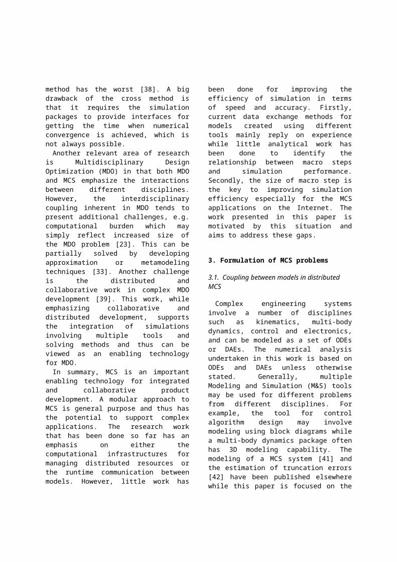
Without lost of generality, Figure 1 shows a cou-pling system with three subsystem models, namely S1, S2, and S3, each of which is created and solved us-

ing a specific M&S engine and runs at different sites. The development of such a system generally involves two key issues [41]. The first issue is the construction of subsystem models, which aims to identify the de-sign variable vectors (z1, z2, and z3) and the system functions (f1, f2, and f3) based on assumptions made for, and physical rules in, each individual discipline. This task can now be well assisted by M&S tools which can transform diagrams or 3D models into DAEs or ODEs. The second issue is to identify the coupling relationships between the models, e.g. Y12

in the figure which denotes the outputs from S1 to S2. The coupling relationships can be vital for the fol-lowing issues that influence the performance of a simulation such as the order of starting the integra-tion processes of the models, the selection of macro time steps, and the methods for eliminating (or miti-gating the effects of) problems such as algebraic loops. Based on the above discussion, a coupling MCS system then can be described using Eq. (1) where z(t) denotes the design variable vectors of the whole system and t denotes time. Thus subsystem models can be obtained by dividing the equation as two or more equations with coupling variables.

(1)

For the sake of simplicity, the coupling and inter-action between two subsystem models are investi-gated throughout this paper while the cases with more than two models can be addressed in the same way as the methods developed are not dependent upon the number of subsystems. The equations for the two subsystem models, namely z1(t) and z2(t), are shown in Eqs. (2) and (3) where y1 and y2 denote the output functions of z1(t) and z2(t). M and N are the size of vectors z1(t) and z2(t) and M+N means the size of vector z(t) in Eq. (1). Similarly, S and T are the size of vectors Y12(t) and Y21(t). Then the solving of the coupled system can be done by performing nu-merical integration for the two models in parallel and exchanging data at regular intervals.

(2)

(3)

Fig. 1. The coupling between subsystem models in MCS

3.2. The numerical integration process of a MCS problem

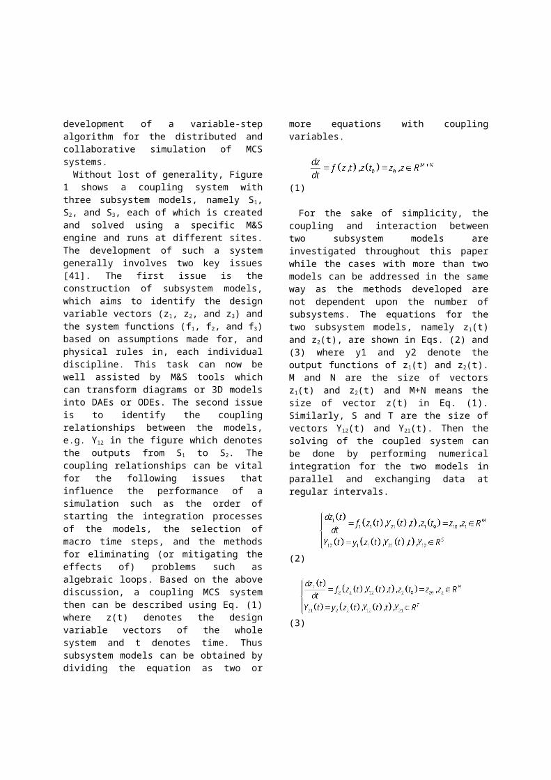
As discussed in Section 3.1, the numerical integra-tion process of a coupled system can be viewed as a process of data exchange between two models de-scribed using Eqs. (2) and (3) which are then solved in parallel using different integration methods with different time steps. This process is illustrated in Fig-ure 2 where subsystems S1 and S2 are solved using two different solvers and the inputs/outputs (i.e. Y12

and Y21) between them are dispatched by a discrete scheduler. Moreover, the discrete scheduler also con-trols the simulation time of the whole system by re-quiring the two models to perform numerical integra-tion for a macro step H, i.e. from ti to ti+1, as shown on the right of Figure 2. Within each macro step, the integration process of each model may involve sev-eral micro steps, i.e. h1j and h2j in the figure, which

are used by the solvers for specific models and there-fore can be different from each other.

Generally, only data at macro steps are exchanged due to two main reasons. Firstly, it is not efficient to perform too many exchanges during the simulation process especially in a distributed environment. Sec-ondly, some M&S tools do not provide the interfaces for accessing simulation data at micro steps. The is-sue of finding the approximations of Y12 and Y21 at micro steps thus arises, which is vital to simulation accuracy. A method for this issue is to use interpola-tion/extrapolation to find data at the current step on the basis of the data obtained from the previous steps. In Figure 2, I(Y21(t)) and I(Y12(t)) are the interpola-tion functions used by each subsystem to calculate the values of Y21 and Y12 at time ti+1 using their values at the previous steps, i.e. Y21k and Y12k (k=0,1,…, i). There are a number of effective interpolation meth-ods and the Lagrange method is the one commonly used. If the Lagrange method is used, the approxi-mated values of Y12 and Y21 can be calculated using Eqs. (4) and (5) where interpolation basis Lk(t) can be calculated using Eq. (6). Figure 3 shows the approxi-mation of Y21 using interpolation where the solid curve consists of the real values and the dashed curve represents the approximated values.

(4)

(5)

(6)

Fig. 2. Runtime interaction between two subsystem models

Two key issues, therefore, need to be addressed to achieve accurate, effective and efficient simulation for MCS. Firstly, an appropriate macro step H needs to be selected to enable a simulation to achieve an ac-ceptable accuracy yet running at a fast speed. Sec-ondly, effective interpolation methods need to be used to find approximated values of input/output data at micro steps. The use of a fixed macro step H for the whole simulation process has two drawbacks. On the one hand, the selection of H largely depends on experience and may involve many numbers of itera-tion. On the other hand, it is not sensible to use a fixed H in terms of simulation efficiency. For exam-ple, it is not necessary to use a big H when the values of design variables only change at a slow pace. It is, therefore, useful to develop a variable-step interac-tion algorithm. An immediate issue raised is the esti-mation of local truncation errors, which holds the key to selecting an appropriate H for the current time step. Moreover, the order of the interpolation meth-ods used needs to be traded off against simulation ef-ficiency and numerical stability. These issues need to be well addressed in the development.

Fig. 3. Interpolation for finding approximated values of Y2

4. Local truncation error estimation

In numerical calculation, a Local Truncation Error (LTE) comes from the finite number of steps in the computation performed by numerical algorithms to obtain approximated values. As discussed above, the estimation of LTE is the key to selecting an appropri-ate macro step H. It is therefore critical to the integra-tion process which is controlled by variable-step al-gorithms for both a single system and MCS. For the former, LTE is mainly determined by the numerical

integration algorithm used for the system while LTEs of the latter depend on both the integration errors and the errors introduced by the interpolation and extrap-olation methods. In this section, the methods for esti-mating the LTEs for both the two cases are dis-cussed.

4.1. LTE for the simulation of a single system

Take the system described in Eq. (1) as an exam-ple, the variable-step integration algorithm for such a system does not need to take into account the interac-tion between subsystem models and the integration step size is solely determined by the errors caused by the numerical integration methods used. Richardson developed a method to solve differential equations by using approximate form of difference equations [21]. This is called the Richardson extrapolation method which can be used for calculating LTEs for a single system in two main steps. Assume z(tk) and z(tk+1) are the real values of vari-able z at time points tk and tk+1, respectively, while zk

and zk+1 denote their approximations obtained using numerical integration. The difference between z(tk+1) and zk+1 is the LTE at time tk+1. Likewise, the differ-ence between z(tk) and zk is the error at time tk. Mark the value of obtained z at step k+1 and calculated us-ing an integration step h as z[h]

k+1 and the one calcu-lated using two h/2 integration steps as z[h/2]

k+1, then the LTE for this case can be calculated using Eqs. (7) and (8), where p is the order of the numerical method used in the integration. Thus LTE can be identified on the basis of different values for h as p can be viewed as a constant which only depends on the spe-cific integration method used. Although this method involves the extra calculation for z[h/2]

k+1, it, however, provides a straightforward LTE calculation method whereby the values for h can be adjusted at runtime according both the specific LTEs of the design vari-ables and the maximum tolerances specified for the whole problem.

(7)

(8)

4.2. LTE for MCS problems

The evaluation of the LTEs for MCS problems is more complex because they also involve the errors caused by the interpolation methods used for obtain-ing the approximations of the data from other mod-els, in addition to the errors from the integration methods. For the sake of brevity, the LTE of a single model will be analyzed in this section and the same process can be applied to other models. Take subsys-tem S1 in Section 3 as an example, its inputs are calculated using Eq. (5) on the basis of the inputs

it gets from subsystem S2. Assume the input vectors for S1 at ti+1, ti, ti-1…ti-n are , , and , respectively, then the error of z1 can be calculated us-ing Eq. (9) where and are the increment func-tions for calculating and . Then, the errors caused by the integration and interpolation methods can be shown as the left-hand sides of Eqs. (10) and (11), respectively. Readers interested in the detailed derivation process of the formulas are referred to [42].

(9)

(10)

(11)

The LTE for S1, thus, can be denoted as Eq. (12) which includes two parts, namely the cumulative in-tegration error generated by the integration method used for S1, and the interpolation error generated by the interpolation method used for calcu-lating on the basis of the inputs from S2.

(12)

In this work, the application of the Richardson ex-trapolation is extended from a single system to a cou-pled system such as MCS to derive the formulas for calculating the errors shown in Eqs. (10) through to (12). The detailed derivation process of the formulas is out of the scope of this paper and has been pub-lished elsewhere [42]. Likewise, the calculation of LTEs for MCS problems also involves two steps of obtaining the results at step H/2 and H, respectively. This paper, mainly focusing on the development of a

variable-step interaction algorithm, only highlights the main findings of the derived formulas without de-tailed discussions on the derivation process, and in-terested readers are referred to [39] for more details. Mark as the order of the integration method and

as the order of the interpolation method, then the LTE of a MCS problem can be calculated in a num-ber of different ways in terms of the various relation-ships between these two parameters:

(1). When , Eq. (13) can be used. This is the situation where the integration error dominates and the influence of the interpolation error can be omitted.

(13)

(2). When , Eq. (14) can be used where Sa and Sb are calculated using Eqs. (15) and (16), re-spectively. This is the situation in which the order of the integration method is very high and its error can therefore be omitted.

(14)

(15)

(16)

The variables Si, Si-1 and their derivations can be calculated using Eqs. (17) through to (19), which de-note the ratio of the current simulation step Hi to the previous simulation steps Hi-1.

(17)

(18)

(19)

(3). When and (this condition can be met if a zero-order interpolation method and an one-order integration method are used, i.e., when

, and ), the formula for the LTE of subsystem S1 can then be calculated using Eq. (20).

(20)

(4). When , and (this condition can be met if the interpolation method’s order is larger than zero), the formula for the LTE of subsys-tem S1 can then be obtained using one of two meth-ods as follows: firstly, dividing the second half of the integration step into two smaller parts for which further calculations will be performed; and secondly, using the other two points within Hi to perform the calculation.

Likewise, the LTEs of subsystem S2 can also be calculated. Thus, the LTEs for different variables in a MCS system can be calculated at simulation runtime and compared with the maximum tolerances. Based on the comparison, the appropriate step sizes can be determined in an automatic and dynamic manner at different points of the simulation process without compromising the accuracy of simulation.

5. A variable-step algorithm for MCS

As discussed in the previous section, LTEs of the design variables in a MCS system are dependent on the simulation step H and the orders (i.e. p1 and q2) of both the integration and the interpolation methods. If the system changes very fast, i.e. the difference be-tween z[H/2]

k+1 and z[H]k+1 is large, then the LTE is large

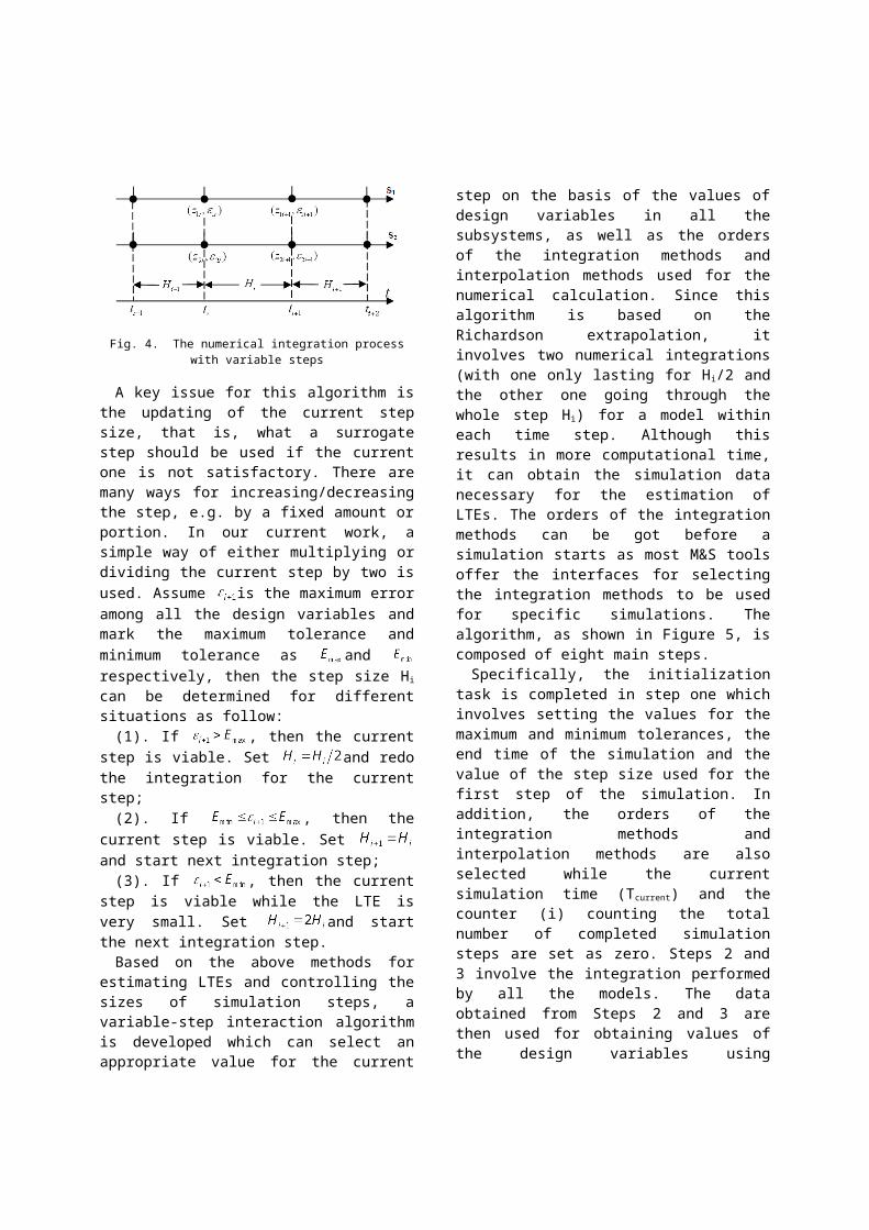
and a small step H is needed. On the other hand, a small step H is not necessarily needed when the sys-tem changes at a slow pace. In the latter circum-stance, the use of a small step results in the increase of the number of total steps of simulation. The ad-verse effects of this increase become more prominent when a MCS runs in a distributed environment, mak-ing the development of a variable-step interaction al-gorithm for distributed MCS a necessity. Figure 4 shows the integration processes of the subsystem models in a MCS problem with variable steps (i.e. Hi-

1, Hi and Hi+1) for data exchange between the models. The size of each step is determined at runtime based on the estimation of LTEs. At the beginning of each step, a provisional step is used first to perform the in-tegration and the resultant LTEs are evaluated. A de-cision will be made on whether to use a surrogate step and this process will be repeated until a satisfac-tory step size is obtained.

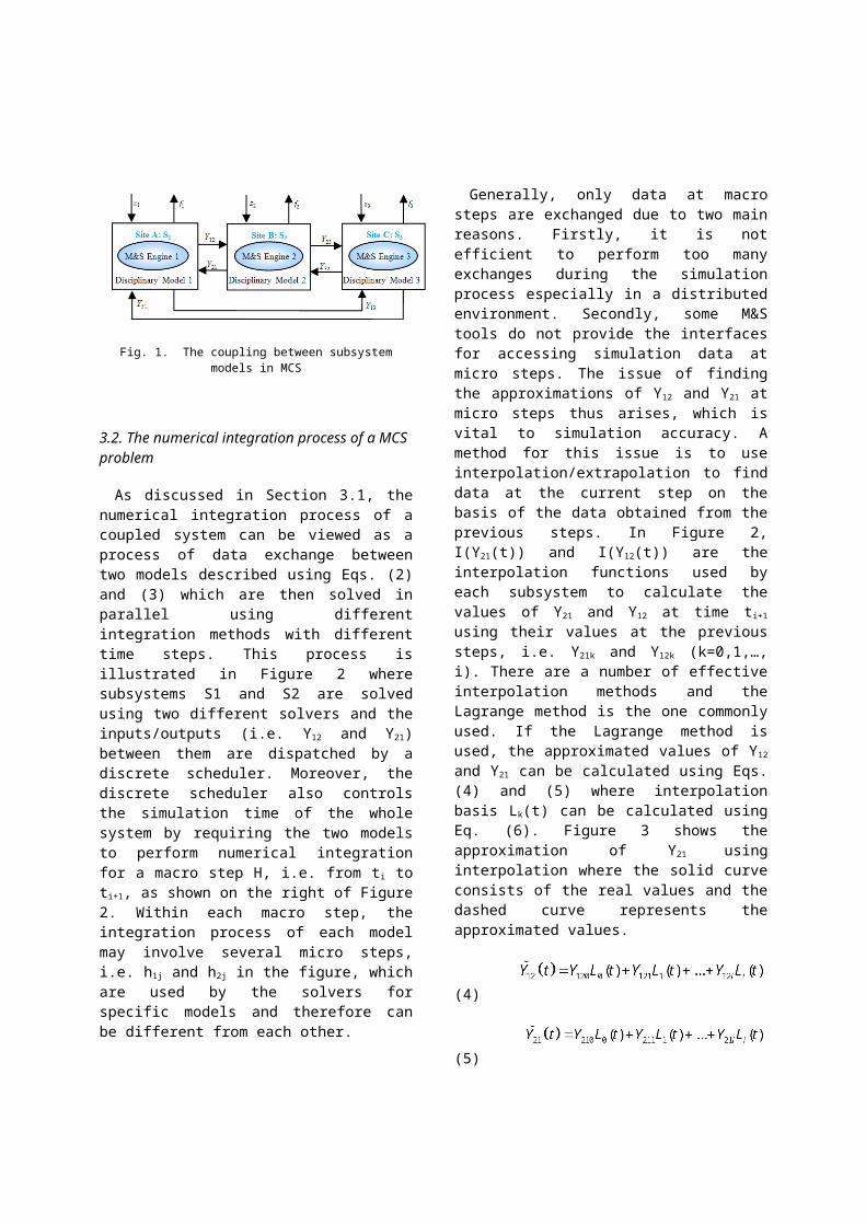
Fig. 4. The numerical integration process with variable steps

A key issue for this algorithm is the updating of the current step size, that is, what a surrogate step should be used if the current one is not satisfactory. There are many ways for increasing/decreasing the step, e.g. by a fixed amount or portion. In our current work, a simple way of either multiplying or dividing the current step by two is used. Assume is the maximum error among all the design variables and mark the maximum tolerance and minimum tolerance as and respectively, then the step size Hi can be determined for different situations as follow:

(1). If , then the current step is viable. Set and redo the integration for the current step;

(2). If , then the current step is vi-able. Set and start next integration step;

(3). If , then the current step is viable while the LTE is very small. Set and start the next integration step.

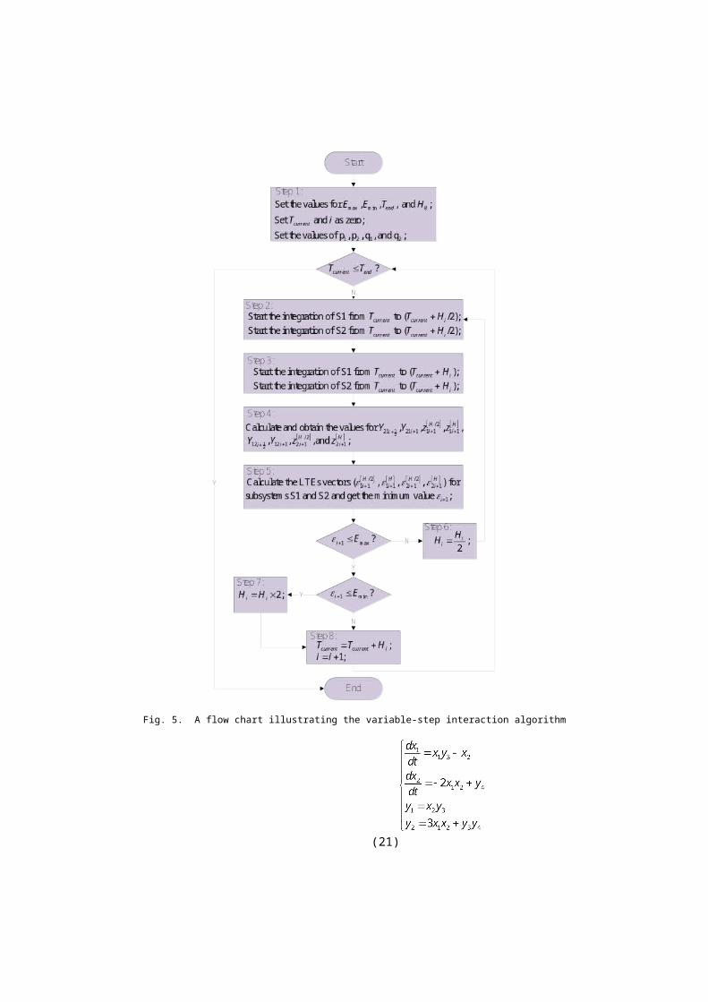
Based on the above methods for estimating LTEs and controlling the sizes of simulation steps, a vari-able-step interaction algorithm is developed which can select an appropriate value for the current step on the basis of the values of design variables in all the subsystems, as well as the orders of the integration methods and interpolation methods used for the nu-merical calculation. Since this algorithm is based on the Richardson extrapolation, it involves two numeri-cal integrations (with one only lasting for H i/2 and the other one going through the whole step H i) for a model within each time step. Although this results in more computational time, it can obtain the simulation data necessary for the estimation of LTEs. The orders of the integration methods can be got before a simu-lation starts as most M&S tools offer the interfaces for selecting the integration methods to be used for specific simulations. The algorithm, as shown in Fig-ure 5, is composed of eight main steps.

Specifically, the initialization task is completed in step one which involves setting the values for the

maximum and minimum tolerances, the end time of the simulation and the value of the step size used for the first step of the simulation. In addition, the orders of the integration methods and interpolation methods are also selected while the current simulation time (Tcurrent) and the counter (i) counting the total number of completed simulation steps are set as zero. Steps 2 and 3 involve the integration performed by all the models. The data obtained from Steps 2 and 3 are then used for obtaining values of the design variables using numerical integration/interpolation (Step 4) and calculating LTEs for the design variables using Eqs. (13) through to (20) (Step 5). The minimum LTE, i.e. εi+1 in the figure, is selected from the LTEs obtained in Step 5, which is subsequently compared with the maximum and minimum tolerances. Steps 6 and 7 deal with the updating of step size on the basis of the different ways discussed above. Step 8 advances the simulation by one time step.

6. Evaluation and Discussion

Two examples are used for evaluating the vari-able-step algorithm, namely a numerical example and an engineering example. The first example is a sim-ple coupled system divided into two subsystems that are modeled using the same M&S tool. The second one involves two models that are created using dif-ferent tools. Both of them involve data exchange at runtime with subsystem models running separately. Evaluation is done by comparing the results obtained from the variable-step algorithm with those obtained from the algorithm (called constant-step algorithm in this paper unless otherwise stated) using a constant step, with the aim of identifying whether the former can outperform the latter in terms of simulation time. The criteria for evaluation include accuracy, total number of steps used and computational stability.

6.1. A numerical example

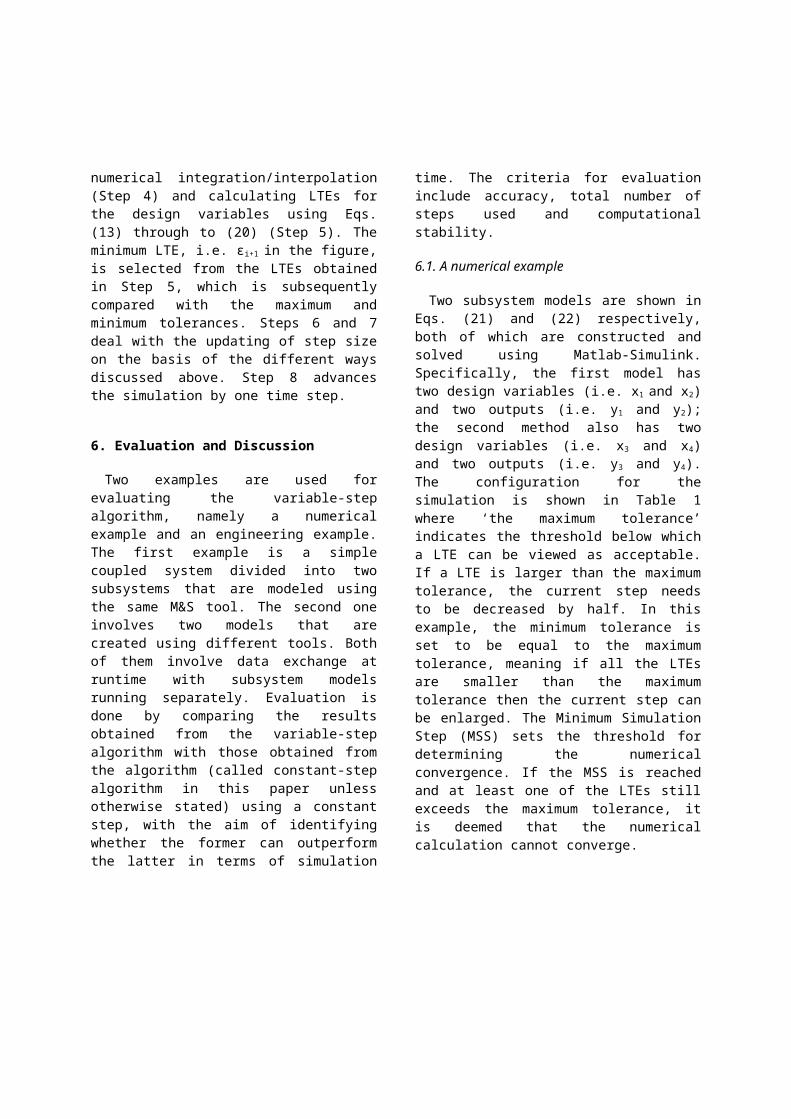
Two subsystem models are shown in Eqs. (21) and (22) respectively, both of which are constructed and solved using Matlab-Simulink. Specifically, the first model has two design variables (i.e. x1 and x2) and two outputs (i.e. y1 and y2); the second method also has two design variables (i.e. x3 and x4) and two out-puts (i.e. y3 and y4). The configuration for the simula-tion is shown in Table 1 where ‘the maximum toler-ance’ indicates the threshold below which a LTE can be viewed as acceptable. If a LTE is larger than the

maximum tolerance, the current step needs to be de-creased by half. In this example, the minimum toler-ance is set to be equal to the maximum tolerance, meaning if all the LTEs are smaller than the maxi-mum tolerance then the current step can be enlarged.

The Minimum Simulation Step (MSS) sets the threshold for determining the numerical convergence. If the MSS is reached and at least one of the LTEs still exceeds the maximum tolerance, it is deemed that the numerical calculation cannot converge.

Fig. 5. A flow chart illustrating the variable-step interaction algorithm

(21)

(22)

Table 1

Simulation configuration for the numerical example

Initial values of variables x1=-1;x2=1;x3=-1;x4=1;y1=-3;y2=6;y3=-3;y4=-3;

Simulation period 0~2 secondsMaximum tolerance 0.01Minimum tolerance 0.01Minimum simulation step 0.001 seconds

Simulation accuracy in this example is evaluated by comparing its results with those (called ‘standard results’ in this paper) obtained from the simulations where a constant-step algorithm is used, as well as with those obtained by performing centralized simu-lation of the whole system in Matlab-Simulink. Specifically, three simulations with different settings are run to evaluate the algorithm under different cir-cumstances where the orders of the integration and interpolation methods are different. It is noteworthy that the orders of the integration and interpolation methods used by a model do not influence the LTEs of other models as they are calculated individually for each model. Therefore, the same integration and interpolation methods are used for the two models in this case. In all the simulations, the variable-step al-gorithm can successfully complete the integration process without encountering numerical instability, and outperform the constant-step algorithms. For the sake of brevity, only the results of variable x3 are an-alyzed for comparison, as shown in Figure 6 where p and q denote the orders of the integration and inter-polation methods respectively.

In the figure, ‘Standard’ means ‘standard results’, ‘Equal’ means the results obtained from a constant-step algorithm and ‘Variable’ means the results ob-

tained from the variable-step algorithm. In all the three simulations, the total numbers of step (the value of ‘step’ in the figure) are nearly the same, which means the total numbers of data exchange are roughly the same. In this case, it is shown that, the variable-step algorithm obtains results comparable to the ‘standard results’ whereas the constant-step algo-rithm gets less accurate results especially in the first two situations. The LTEs of x3 and the values of the variable step for the first model (x3 is one of its design variables) throughout the simulation process are shown in Fig-ure 7 and Figure 8 respectively. For all the cases, the LTEs are always within the maximum limit of 0.01. For the first two cases, the LTEs are generally very big so a big step size (up to 0.08 seconds in simula-tion time) is used by the algorithm where as a small step is mostly used for the third case.

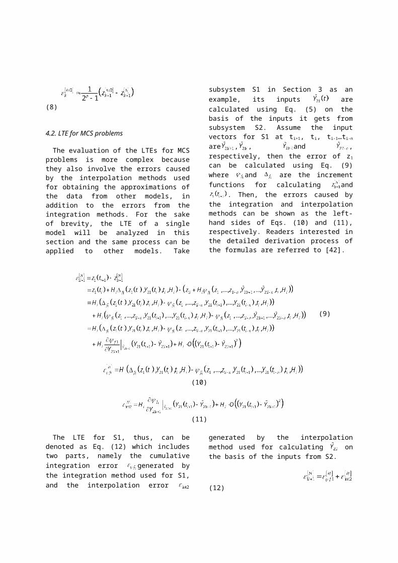
Fig. 6. Comparison of accuracy between the variable-step algo-rithm and a constant-step algorithm

The constant-step algorithm can actually achieve improved accuracy by selecting a smaller size for the constant step. To compare the performance of the two algorithms in terms of the total number of steps involved, a smaller step is used for the constant-step algorithm and the comparison of results for x1 is then shown in Figure 9. It is shown that the variable-step algorithm requires much less number of steps when similar accuracies (the accuracy of the variable-step algorithm is actually still better especially in the third situation) are achieved by the two algorithms. This means a significant saving of total simulation time.

Fig. 7. The LTEs of variable x3 under different circumstances: left (step=49, p=1, q=1), middle (step=75, p=1, q=0), right(step=41,p=4, q=1)

Fig. 8. The variable steps used throughout the simulation process for the three cases

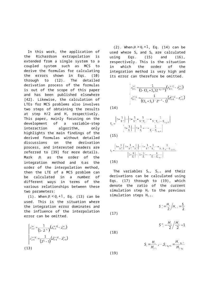
Fig. 9. Comparison of the results for variable x3 when a smaller step is used for the constant-step algorithm

6.2. An engineering example

The engineering example is focused on controlling the tilting process of a satellite with the aim of evalu-ating the variable-step algorithm for the MCS prob-lems involving multiple M&S tools. Specifically, the simulation involves one control model created using Matlab-Simulink and one dynamics model created using MSC.Adams, as shown in Figure 10. The dy-namics model is driven by a control torque applied by the control model and accordingly calculates the resultant azimuth position of the satellite and the ve-

locity of the rotor, both of which are used as the in-puts for the control model. The culmination of the control process is that the satellite is smoothly driven to tilt by a specific angle. An external program is written to control the advancement of the two models and complete the data exchange, implementing the variable-step algorithm. The simulation configuration for this example is shown in Table 2. Three simula-tions, again, are performed for this example under different circumstances where the orders of the inte-gration/interpolation methods are different. As demonstrated in these simulations, the numerical in-tegration processes where the variable-step algorithm is applied are both stable and sufficient. For the sake of brevity, the comparison of the results for control torque is shown in Figure 11. It is demonstrated that the variable-step algorithm outperforms the constant-step algorithm in terms of the total number of steps involved while a comparable accuracy is achieved. The third circumstance with p=4 and q=1, in particu-lar, shows that the variable-step algorithm can save up to 42 steps (about 17%).

Fig. 10: Interaction between subsystem models of a satellite

Table 2

Simulation configuration for the engineering example

Initial values of variables Control_torque = 0.0;Azimuth_position = 0.0;Rotor-Velocity = 0.0;

Simulation period 0~0.25 secondsMaximum tolerance 0.01Minimum tolerance 0.01Minimum simulation step 0.0005 seconds

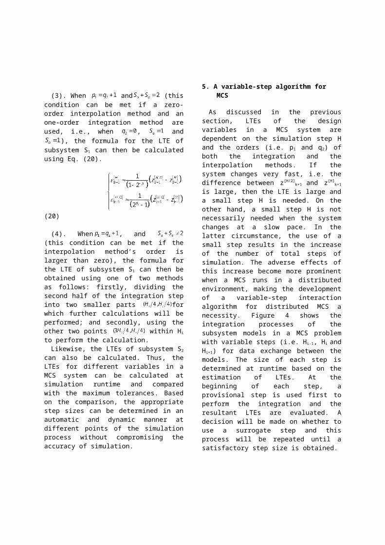
Fig. 11. Comparison of the simulation results for the control torque under different circumstances

6.3. Discussion

As evidenced in both the numerical and engineer-ing examples, the variable-step algorithm is stable, accurate and efficient. Firstly, the step size is selected by the algorithm to ensure LTEs are within the maxi-

mum tolerance, and thus numerical convergence was successfully achieved in all the tests. In this sense, the proposed algorithm is stable. Secondly, the vari-able-step algorithm obtained results with comparable accuracy to the ‘standard results’ while outperform-ing the constant-step algorithms in most cases when a similar number of steps were involved. Therefore, the algorithm is accurate. Thirdly, the variable-step algo-rithm, compared with constant-step algorithms, re-quires less number of steps to complete the running of simulation and thus achieves improved efficiency. For example, the numbers of steps reduced by the variable-step algorithm are 51 (a reduction of 51%), 25 (a reduction of 25%), and 39 (a reduction of 49%) for the three situations (for two of them, similar accu-racies are achieved while for one of them better accu-racy is achieved) in Figure 10, respectively. For the engineering example, the variable-step algorithm also successful reduces the total simulation steps by 16, 12 and 42 respectively, as shown in Figure 12. There-fore, it is shown in all the tests that the proposed al-gorithm has achieved very good performance.

For a distributed MCS, data exchange communi-cation imposes a burden on simulation time as syn-chronizing all subsystems takes a very long time. In this case, the reduction of simulation steps means great saving on the total simulation time and, as such, the advantages of the variable-step algorithm become more prominent. For instance, if it takes 0.5 seconds to complete all the simulation tasks and distributed communication, then nearly a total of 26 seconds can be saved for the situation 1 in Figure 10. This is re-ally a significant improvement to the simulation per-formance. In addition, this algorithm does not require a precise step size to be specified before a simulation starts as the size of steps will be adjusted on the basis of LTE estimation. This makes the configurations of simulations much easier compared with those of con-stant-step algorithms which are error-prone and very much relies on experience.

As the proposed algorithm is for distributed inter-action between computational models, the total simu-lation time is determined by two parts, namely the time taken to complete the simulation of each model and the time taken to complete data exchange com-munication. Generally, the time for initializing M&S engines is much longer than the time for performing numerical integration for a time step, so we can as-sume that the time taken (by a M&S tool) for the nu-merical integration from t to t+H equals that taken (by a M&S tool) for the numerical integration from t to t+H/2. Therefore, the complexity of a constant-

step algorithm can be estimated as a*(ts + tc) where a means the total number of steps taken to complete the whole simulation process and ts and tc represents the time taken to complete numerical integration and data exchange communication, respectively. Like-wise, the complexity of the proposed algorithm can be estimated as b*(2*ts + tc) where b means the total number of steps (ts and tc have the same meanings as the previous expression). The reason ts is multiplied by 2 is because the proposed algorithm involves two times of integrations (to H/2 and to H respectively) in each step.

As mentioned above, in a distributed MCS, tc is much larger than ts and, as such, the complexities ex-pressions for the proposed algorithm and a constant-step algorithm can be marked as a*O(n) and b*O(n), respectively, where n means the total number of sub-systems in a MCS. The variable-step algorithm re-quires less number of simulation steps (i.e. a<b) so in theory it is better in terms of time complexity. More-over, this also indicates the method can be extended to cases with three or more models. The algorithm has been implemented in a working prototype of dis-tributed MCS, on which the engineering example was run. The snapshots of some user interfaces are shown in Figure 12 and currently the system can sup-port distributed MCS and simple post-processing. This further demonstrates that the algorithm is viable and implementable.

Fig. 12. Snapshots of a working prototype

7. Conclusion remarks

In this paper, the development of a variable-step interaction algorithm for MCS in a distributed envi-ronment is presented. This algorithm is aimed at ad-dressing the issues involved in traditional constant-step algorithms, e.g. the selection of an appropriate step and the long simulation time caused by small steps used for achieving numerical stability safely. The selection of a constant simulation step is error-prone and very much replies on experience, and, as such, a safe method is to choose a small one. How-ever, a smaller step means longer running time, which is not acceptable for distributed MCS. There-fore, a variable-step algorithm becomes a necessity and has great potential for improving simulation per-formance.

The key issues involved in the variable-step algo-rithm include the estimation of local truncation error and the strategy for controlling the size of simulation step at runtime. The solutions to these issues are dis-cussed in detail in this paper. Both a numerical exam-ple and an engineering example are used to evaluate the performance of the algorithm. As evidenced in the tests, the variable-step algorithm outperforms constant-step algorithms in terms of both accuracy and efficiency. On the one hand, the algorithm can achieve much better accuracy when the steps used by constant-step algorithms are not big. On the other hand, when constant-step algorithms use very small steps to achieve better accuracy, they will use much more steps than the variable-step algorithm. Little work has been done so far on developing variable-step algorithms for MCS and the current version of the algorithm helps open up such a field which re-quires much further work. In our future work, we will focus on improving the performance of the algo-rithm, e.g. developing better strategy for controlling the size of simulation steps. Also, we will do further simulation experiments to evaluate the stability and robustness of the algorithm.

Acknowledgement

This research is supported by the National Natural Science Foundation of China (Grant Nos. 61074110 and 61374163).

References

[1] H. Adeli and S. Kumar, Distributed Finite Element Analysis on a Network of Workstations - Algorithms, Journal of Struc-tural Engineering, ASCE, 121:10 (1995), pp. 1448-1455.

[2] H. Adeli, and G. Yu, An Integrated Computing Environment for Solution of Complex Engineering Problems Using the Ob-ject-Oriented Programming Paradigm and a Blackboard Ar-chitecture, Computers and Structures, 54:2(1995), pp. 255-265.

[3] J. Ambrósio, J. Pombo, F. Rauter, and M. Pereira, A memory based communication in the co-simulation of multibody and finite element codes for Pantograph-Catenary interaction sim-ulation, Multibody Dynamics, 2008, pp. 231-252.

[4] M. Arnold, Multi-rate time integration for large scale multi-body system models, IUTAM Symposium on Multiscale Problems in Multibody System Contacts, Springer, Nether-lands, 2007, pp. 1-10.

[5] R. Badaway, B. Hirsch, and S. Albayrak, Agent-based coordi-nation techniques for matching supply and demand in energy networks, Integrated Computer-Aided Engineering, 17:4 (2010), 373-382.

[6] A. Bonelli, O.S. Bursi, L. He, G. Magonette, and P. Pegon, Convergence analysis of a parallel interfield method for het-erogeneous simulations with dynamic substructuring, Interna-tional Journal for Numerical Methods in Engineering, 2008, Vol. 75, pp. 800-825.

[7] J. Byrne, C. Heavey, and P. Byrne, A review of Web-based simulation and supporting tools, Simulation Modelling Prac-tice and Theory, 18:3 (2010), 253-276.

[8] L. Cristaldi, F. Ponci, M. Riva, and M. Faifer, Multi-agent systems: an example of power system dynamic reconfigura-tion, Integrated Computer-Aided Engineering, 17:4 (2010), 359-372.

[9] J. Fei, Convergence and convergence order of decomposition methods with interpolations for numerical initial value prob-lems of ordinary differential equations (in Chinese), Numeri-cal Calculation and Computer Application, 12:3 (1994), 209-218.

[10]C.A. Felippa, K.C. Park, and C. Farhat, Partitioned analysis of coupled mechanical systems, Computer Methods in Applied Mechanics and Engineering, 190 (2001), 3247-3270.

[11]A.J. Fougères and E. Ostrosi, “Fuzzy agent-based approach for consensual design synthesis in product configuration,” In-tegrated Computer-Aided Engineering, 20:3(2013), pp. 259-274.

[12]C.W. Gear, D.R. Well, Multirate linear multistep methods, BIT, 24 (1984), 484-502.

[13]M. Grzenda, A. Bustillo, and G. Quintana, and J. Ciurana, “Improvement of surface roughness models for face milling operations through dimensionality reduction,” Integrated Computer-Aided Engineering, 19:2 (2012), 179-198.

[14]J.O. Gutierrez-Garcia and K.M. Sim, Agent-based Cloud Workflow Execution, Integrated Computer-Aided Engineer-ing, 19:1 (2012), 39-56.

[15]B. Johansson, and P. Krus, A Web Service approach for model integration in computational design, Proceedings of the ASME Design Engineering and Technical Conferences & Computers and Information in Engineering Conference (IDETC&CIE 2003), Chicago, USA, September 2003.

[16]R. Kübler and W. Schiehlen, Modular simulation in multibody system dynamics, Multibody System Dynamics 4 (2000), 107-127.

[17]X. Li, F. He, X. Cai, D. Zhang and Y. Chen, “A Method for Topological Entity Matching in the Integration of Heteroge-

neous CAD Systems, Integrated Computer-Aided Engineer-ing, 20:1 (2013), pp. 15-30.

[18]D. López-París, and A. Brazález-Guerra, A new autonomous agent approach for the simulation of pedestrians in urban envi-ronments, Integrated Computer-Aided Engineering, 16:4 (2009), 283-297.

[19]M. Prymek, and A. Horak, Multi-agent approach to power dis-tribution network modelling, Integrated Computer-Aided En-gineering, 17:4 (2010), 291-303.

[20]U. Reuter, A Fuzzy Approach for Modelling Non-stochastic Heterogeneous Data in Engineering Based on Cluster Analy-sis, Integrated Computer-Aided Engineering, 18:3 (2011), 281-289.

[21]L.F. Richardson, The Approximate Arithmetical Solution by Finite Differences of Physical Problems Involving Differential Equations, with an Application to the Stresses in a Masonry Dam, Philosophical Transactions of the Royal Society of Lon-don, Series A 210 (459-470) (1911), 307–357.

[22]K. Rodriguez and A. Al-Ashaab, Knowledge web-based sys-tem architecture for collaborative product development, Com-puters in Industry, 56:1 (2005), 125–40.

[23]J.F. Rodríguez, J.E. Renaud, B.A. Wujek and R.V. Tappeta, Trust region model management in multidisciplinary design optimization, Journal of Computational and Applied Mathe-matics, 124:1-2 (2000), 139-154.

[24]G.S. Ryu, Integration of heterogeneous simulation models for network-distributed simulation, Ph.D. Dissertation, University of Michigan, 2009.

[25]J. Samin, O. Brüls, J. Collard, L. Sass and P. Fisette, Multi-physics modeling and optimization of mechatronic multibody systems, Multibody System Dynamics, 18:3 (2007), 345-373.

[26]J. Sedano, A. Berzosa, J.R. Villar, E.S. Corchado, and E. de la Cal, Optimising operational costs using Soft Computing tech-niques, Integrated Computer-Aided Engineering, 18:4 (2011), 313-325.

[27]N. Senin, D.R. Wallace and N. Borland, distributed object-based modeling in design simulation marketplace, Transaction of the ASME, Journal of Mechanical Design, 125:1 (2003), 2–13.

[28]W. Shen et al., Systems integration and collaboration in archi-tecture, engineering, construction, and facilities management: a review”, Advanced Engineering Informatics, 24:2 (2000), 196-207.

[29]S.S. Shome, E.J. Haug, and L.O. Jay, Dual-rate integration us-ing partitioned Runge-Kutta methods for mechanical systems with interacting subsystems, Mechanics Based Design Of Structures And Machines, 32 (2004), 253-282.

[30]J. Solanki, S.K. Solanki and N. Schulz, Multi-agent-based re-configuration for restoration of distribution systems with dis-tributed generators, Integrated Computer-Aided Engineering, 17:4 (2010), 331-346.

[31]H. Sun, W. Fan, W. Shen, T. Xiao, and Y. Chai, Ontology Maintenance in High Level Architecture Federation Develop-ment and Execution Process, Integrated Computer-Aided En-gineering, 20:1 (2013), 79-94.

[32]G. Vigueras, J.M. Orduna, M. Lozano, and Y. Chrysanthou, A Distributed Visualization System for Crowd Simulations, Inte-grated Computer-Aided Engineering, 18:4 (2011), 349-363.

[33]G.G. Wang and S. Shan, Review of Metamodeling Tech-niques in Support of Engineering Design Optimization, Trans-action of the ASME, Journal of Mechanical Design, 129:4 (2007), 370–380.

[34]H. Wang, A. Johnson and H. Zhang, The assembly of compu-tational models for the collaborative development of virtual prototypes, Proceedings of the ASME Design Engineering and Technical Conferences & Computers and Information in Engi-

neering Conference (IDETC&CIE 2009), San Diego, Califor-nia, USA, September 2009.

[35]H. Wang A. Johnson, H. Zhang and S. Liang, Towards a col-laborative modeling and simulation platform on the Internet, Advanced Engineering Informatics, 24:2 (2010), 208-218.

[36]H. Wang and H. Zhang, A distributed and interactive system to integrated design and simulation for collaborative product development, Robotics and Computer-Integrated Manufactur-ing, 26:6 (2010), 778-789.

[37]H. Wang, and H. Zhang, An integrated and collaborative ap-proach for complex product development in distributed het-erogeneous environment, International Journal of Production Research, 46: 9 (2008), 2345-2361.

[38]H. Wang and H. Zhang, A study on the runtime interaction be-tween distributed computational models in multidisciplinary collaborative simulation, Proceedings of the 2010 IEEE Inter-national Conference on Systems, Man, and Cybernetics (IEEE SMC), Istanbul, Turkey, October 2010.

[39]Y.D. Wang, W. Shen and H. Ghenniwa, WebBlow: a Web/agent-based multidisciplinary design optimization environ-ment, Computers in Industry, 52:1 (2003), 17-28.

[40]H. Zhang, A solution of multidisciplinary collaborative simu-lation for complex engineering systems in a distributed hetero-geneous environment, Science China Information Sciences, 52:10 (2009), 1848-1862.

[41]H. Zhang, P. Cui, C. Zhang and H. Wang, A variable-step nu-merical method for collaborative computation of two coupling models in multidisciplinary engineering systems, Proceedings of the 2011 IEEE International Conference on Computer Sup-ported Cooperative Work in Design (IEEE CSCWD), Lau-sanne, Switzerland, May, 2011.

[42]H. Zhang, S. Liang, S. Song and H. Wang, Truncation error calculation based on Richardson extrapolation for variable-

step collaborative simulation, Science China Information Sci-ences, 54:6 (2011), 1238-1250.

[43]H. Zhang, H. Wang, D. Chen, and G. Zacharewicz, A model-driven approach to multidisciplinary collaborative simulation for virtual product development, Advanced Engineering Infor-matics, 24:2 (2010), 167-179.

[44]X. Zhang, Y. Li, S. Zhang and C.M. Schlick, Modelling and Simulation of the Task Scheduling Behavior in Collaborative Product Development Process, Integrated Computer-Aided Engineering, 20:1 (2013), 31-44.

[45]F. Zorriassatine, C. Wykes, R. Parkin and N. Gindy, A survey of virtual prototyping techniques for mechanical product de-velopment, Proceedings of the Institution of Mechanical Engi-neers, Part B: Journal of Engineering Manufacture, 217:4 (2003), 513-530.