Embed Size (px)
Citation preview

Institutionen för systemteknikDepartment of Electrical Engineering
Examensarbete
State Estimation of UAV using Extended KalmanFilter
Examensarbete utfört i Reglerteknikvid Tekniska högskolan vid Linköpings universitet
av
Thom Magnusson
LiTH-ISY-EX--13/4662--SE
Linköping 2013
Department of Electrical Engineering Linköpings tekniska högskolaLinköpings universitet Linköpings universitetSE-581 83 Linköping, Sweden 581 83 Linköping


State Estimation of UAV using Extended KalmanFilter
Examensarbete utfört i Reglerteknikvid Tekniska högskolan i Linköping
av
Thom Magnusson
LiTH-ISY-EX--13/4662--SE
Handledare: Manon Kokisy, Linköpings universitet
Magnus DegerfalkInstrument Control Sweden
Examinator: Fredrik Gustafssonisy, Linköpings universitet
Linköping, 21 May, 2013


Avdelning, InstitutionDivision, Department
Division of Automatic ControlDepartment of Electrical EngineeringLinköpings universitetSE-581 83 Linköping, Sweden
DatumDate
2013-05-21
SpråkLanguage
Svenska/Swedish Engelska/English
RapporttypReport category
Licentiatavhandling Examensarbete C-uppsats D-uppsats Övrig rapport
URL för elektronisk versionhttp://www.control.isy.liu.se
http://www.ep.liu.se
ISBN—
ISRNLiTH-ISY-EX--13/4662--SE
Serietitel och serienummerTitle of series, numbering
ISSN—
TitelTitle State Estimation of UAV using Extended Kalman Filter
FörfattareAuthor
Thom Magnusson
SammanfattningAbstract
In unmanned systems an autopilot controls the outputs of the vehicle withouthuman interference. All decisions made by the autopilot will depend on estimatesdelivered by an Inertial Navigation System, INS. For the autopilot to take correctdecisions it must rely on correct estimates of its orientation, position and velocity.Hence, higher performance of the autopilot can be achieved by improving its INS.Instrument Control Sweden AB has an autopilot developed for fixed wing aircraft.The focus of this thesis has been on investigating the potential benefits of usingExtended Kalman filters for estimating information required by the control systemin the autopilot. The Extended Kalman filter is used to fuse sensor measurementsfrom accelerometers, magnetometers, gyroscopes, GPS and pitot tubes. The filterwill be compared to the current Attitude and Heading Reference System, AHRS, tosee if better results can be achieved by utilizing sensor fusion.
NyckelordKeywords key1, key2


AbstractIn unmanned systems an autopilot controls the outputs of the vehicle withouthuman interference. All decisions made by the autopilot will depend on estimatesdelivered by an Inertial Navigation System, INS. For the autopilot to take correctdecisions it must rely on correct estimates of its orientation, position and velocity.Hence, higher performance of the autopilot can be achieved by improving its INS.Instrument Control Sweden AB has an autopilot developed for fixed wing aircraft.The focus of this thesis has been on investigating the potential benefits of usingExtended Kalman filters for estimating information required by the control systemin the autopilot. The Extended Kalman filter is used to fuse sensor measurementsfrom accelerometers, magnetometers, gyroscopes, GPS and pitot tubes. The filterwill be compared to the current Attitude and Heading Reference System, AHRS,to see if better results can be achieved by utilizing sensor fusion.
v


Acknowledgments
I would like to send my appreciation to everyone at Instrument Control SwedenAB for providing me with the opportunity to do this master thesis. Thanks toMagnus Degerfalk, supervisor at Instrument Control Sweden AB, for all supportand guidance. I would also like to thank Manon Kok, supervisor at Linköping Uni-versity, for always having time for questions and for providing me with new ideas.I have also had great support from my examiner, Fredrik Gustafsson, LinköpingUniversity, and would like to thank him as well for helping me during this thesis.
vii

Contents
1 Introduction 11.1 Background . . . . . . . . . . . . . . . . . . . . . . . . . . . . . . . 11.2 Motivation . . . . . . . . . . . . . . . . . . . . . . . . . . . . . . . 21.3 Hardware . . . . . . . . . . . . . . . . . . . . . . . . . . . . . . . . 3
2 Coordinate systems 52.1 Earth-Centered, Earth-Fixed . . . . . . . . . . . . . . . . . . . . . 52.2 Local Geodetic Frame . . . . . . . . . . . . . . . . . . . . . . . . . 7
2.2.1 Velocity relations to WGS . . . . . . . . . . . . . . . . . . . 82.3 Body frame . . . . . . . . . . . . . . . . . . . . . . . . . . . . . . . 92.4 Rotation between frames . . . . . . . . . . . . . . . . . . . . . . . . 10
2.4.1 Euler angles . . . . . . . . . . . . . . . . . . . . . . . . . . . 102.4.2 Direction cosine matrix . . . . . . . . . . . . . . . . . . . . 132.4.3 Quaternions . . . . . . . . . . . . . . . . . . . . . . . . . . . 14
3 Sensors 193.1 Gyroscopes . . . . . . . . . . . . . . . . . . . . . . . . . . . . . . . 19
3.1.1 Performance . . . . . . . . . . . . . . . . . . . . . . . . . . 193.1.2 Statistical analysis . . . . . . . . . . . . . . . . . . . . . . . 203.1.3 Calibration . . . . . . . . . . . . . . . . . . . . . . . . . . . 21
3.2 Accelerometer . . . . . . . . . . . . . . . . . . . . . . . . . . . . . . 233.2.1 Performance . . . . . . . . . . . . . . . . . . . . . . . . . . 233.2.2 Statistical analysis . . . . . . . . . . . . . . . . . . . . . . . 233.2.3 Calibration . . . . . . . . . . . . . . . . . . . . . . . . . . . 24
3.3 Magnetometer . . . . . . . . . . . . . . . . . . . . . . . . . . . . . . 253.3.1 Anisotropic Magnetoresistive elements . . . . . . . . . . . . 273.3.2 Measurement errors . . . . . . . . . . . . . . . . . . . . . . 273.3.3 Calibration . . . . . . . . . . . . . . . . . . . . . . . . . . . 293.3.4 Calibration algorithm using least squares . . . . . . . . . . 303.3.5 Calibration results . . . . . . . . . . . . . . . . . . . . . . . 32
3.4 Pressure sensors . . . . . . . . . . . . . . . . . . . . . . . . . . . . 323.4.1 Performance . . . . . . . . . . . . . . . . . . . . . . . . . . 333.4.2 Calibration . . . . . . . . . . . . . . . . . . . . . . . . . . . 33
3.5 GNSS . . . . . . . . . . . . . . . . . . . . . . . . . . . . . . . . . . 34
ix

x Contents
3.5.1 Position estimation . . . . . . . . . . . . . . . . . . . . . . . 343.5.2 Speed and direction estimation . . . . . . . . . . . . . . . . 34
4 Modelling 374.1 Height estimation model . . . . . . . . . . . . . . . . . . . . . . . . 384.2 INS state space models . . . . . . . . . . . . . . . . . . . . . . . . . 39
4.2.1 Measurement equations . . . . . . . . . . . . . . . . . . . . 424.2.2 Gyroscopes . . . . . . . . . . . . . . . . . . . . . . . . . . . 424.2.3 Accelerometers . . . . . . . . . . . . . . . . . . . . . . . . . 424.2.4 Magnetometer . . . . . . . . . . . . . . . . . . . . . . . . . 444.2.5 Pitot tubes . . . . . . . . . . . . . . . . . . . . . . . . . . . 444.2.6 GPS . . . . . . . . . . . . . . . . . . . . . . . . . . . . . . . 45
4.3 Wind estimation model . . . . . . . . . . . . . . . . . . . . . . . . 454.3.1 Measurement equations . . . . . . . . . . . . . . . . . . . . 45
4.4 Models with input signals . . . . . . . . . . . . . . . . . . . . . . . 464.5 Linearization and discretization . . . . . . . . . . . . . . . . . . . . 47
5 Filtering 495.1 Kalman filtering . . . . . . . . . . . . . . . . . . . . . . . . . . . . 49
5.1.1 Kalman filter . . . . . . . . . . . . . . . . . . . . . . . . . . 505.1.2 Extended Kalman filter . . . . . . . . . . . . . . . . . . . . 505.1.3 Iterated Kalman filter . . . . . . . . . . . . . . . . . . . . . 51
5.2 Recursive Least Squares . . . . . . . . . . . . . . . . . . . . . . . . 52
6 Results 556.1 Perturbed magnetic fields . . . . . . . . . . . . . . . . . . . . . . . 55
6.1.1 Electrical disturbances . . . . . . . . . . . . . . . . . . . . . 556.1.2 Small airframes . . . . . . . . . . . . . . . . . . . . . . . . . 566.1.3 Disturbance analysis . . . . . . . . . . . . . . . . . . . . . . 576.1.4 Minimizing electrical disturbances . . . . . . . . . . . . . . 58
6.2 GPS issues . . . . . . . . . . . . . . . . . . . . . . . . . . . . . . . 596.2.1 GPS Modes . . . . . . . . . . . . . . . . . . . . . . . . . . . 596.2.2 Variable latency . . . . . . . . . . . . . . . . . . . . . . . . 616.2.3 GPS conclusions . . . . . . . . . . . . . . . . . . . . . . . . 62
6.3 22 state EKF . . . . . . . . . . . . . . . . . . . . . . . . . . . . . . 626.3.1 Position and Velocity estimation . . . . . . . . . . . . . . . 626.3.2 Attitude estimation . . . . . . . . . . . . . . . . . . . . . . 636.3.3 Bias estimation . . . . . . . . . . . . . . . . . . . . . . . . . 64
6.4 EKF wind estimation . . . . . . . . . . . . . . . . . . . . . . . . . 656.5 RLS parameter estimation . . . . . . . . . . . . . . . . . . . . . . . 66
7 Conclusions and future work 697.1 Conclusions . . . . . . . . . . . . . . . . . . . . . . . . . . . . . . . 697.2 Future work . . . . . . . . . . . . . . . . . . . . . . . . . . . . . . . 70
Bibliography 71

Contents xi
A Linearization 73


Chapter 1
Introduction
1.1 Background
Unmanned Aerial Vehicles, UAV, have been developed since the first world war.At this time they were used as target drones to train anti-air crews and they werecontrolled remotely from the ground. The development of the conventional UAV,as we know it today, was set in motion by United States Air Force, USAF, in1959 to avoid casualties during air surveillance. Since then there has been animmense effort to improve their capabilities. At this time, the components neededto build a UAV were extremely expensive and navigation precision was poor. Inabsence of a Global Navigation Satellite System, GNSS, the UAV had to relyon an Inertial Navigation System, INS, for long range flights. This generated agreat effort in developing an INS, which is using accelerometers and gyroscopes todetermine attitude, velocities and position. Consequently the first generations ofsurveillance UAVs did not succeed in taking photos at the correct locations. Oneof the first navigational improvements was achieved when implementing a Dopplernavigation radar to the UAVs. This type of UAV was flown in 1968.
When the American GNSS, Global Positioning System, GPS, was developedand live feeds from on-board cameras could be transmitted to the ground, themodern UAV as we know it today was developed. At the same time, technologicalimprovements allowed for higher precision UAVs and the price on vital componentssuch as high precision gyroscopes and accelerometers started to drop. This newpossibility of developing cheaper and more effective UAVs has created interest inthe civil market. Today, UAVs are being used in a variety of areas from livestockmonitoring to hurricane research.
These new markets have generated a need for cheap and easy to use UAVs.With the arrival of smaller and cheaper sensors the competition of creating cheap,small and reliable UAVs has grown. Therefore it is now important to developreliable control and navigation systems with commercially available sensors.
1

2 Introduction
Figure 1.1. The ground control station developed by Instrument Control Sweden.
1.2 Motivation
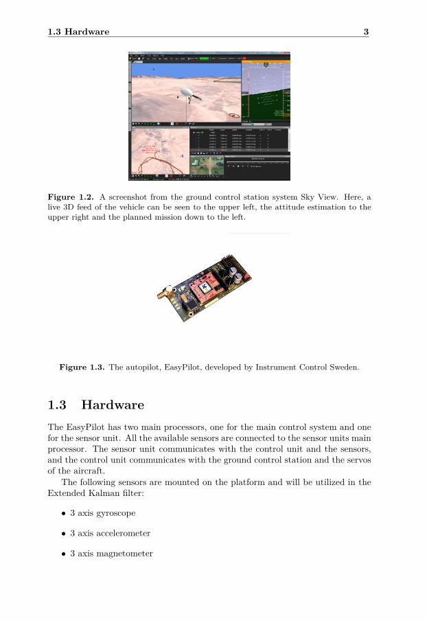
Instrument Control Sweden develops and sells complete solutions for UAV opera-tion with ground control stations, autopilot and high end software. The UnmannedAircraft System, SkyView, allows the user to control and manage several UAVs.The ground control station can be seen in Figure 1.1 and the SkyView user in-terface in Figure 1.2. The autopilot developed by Instrument Control Sweden iscalled EasyPilot and can be seen in Figure 1.3.
It is from SkyView the user decides what the UAV is going to do. From herethe UAV can be controlled in a stabilized mode and mission mode. In stabilizedmode the user controls the UAV directly from the ground station. In this case,EasyPilot controls the aircraft while the user indicates what he wants the aircraftto do. In mission mode a flight path is uploaded to EasyPilot. EasyPilot thencontrols the aircraft to follow the uploaded flight path.
To be able to control the aircraft efficiently, information about attitude, head-ing, position and velocities are required. If incorrect attitude estimations areacquired the performance of the control loops are irrelevant. All this informationis delivered by EasyPilot’s sensor unit. The main goal of this master thesis is toimprove this sensor unit and to enable the control system to work more efficiently.
The main idea is to use an Extended Kalman Filter, EKF, for state estima-tion. An EKF is a powerful way to utilize and merge information from severaldifferent sensors, and still take system dynamics into account. When developingan Extended Kalman filter state dynamics must be derived. Then a mathematicalrelation between sensor measurements and state dynamics are defined. The statedynamics then propagates with time and at every measurement the state dynamicsare updated to minimize the deviation from the true states.
1.3 Hardware 3
Figure 1.2. A screenshot from the ground control station system Sky View. Here, alive 3D feed of the vehicle can be seen to the upper left, the attitude estimation to theupper right and the planned mission down to the left.
Figure 1.3. The autopilot, EasyPilot, developed by Instrument Control Sweden.
1.3 HardwareThe EasyPilot has two main processors, one for the main control system and onefor the sensor unit. All the available sensors are connected to the sensor units mainprocessor. The sensor unit communicates with the control unit and the sensors,and the control unit communicates with the ground control station and the servosof the aircraft.
The following sensors are mounted on the platform and will be utilized in theExtended Kalman filter:
• 3 axis gyroscope
• 3 axis accelerometer
• 3 axis magnetometer

4 Introduction
Figure 1.4. The Spy Owl 100 is a UAV designed for training purposes. It is a rigidconstruction on which the EasyPilot has been developed and evaluated.
• GPS
• Static and dynamic pressure sensors
The current processor mounted on the chip is a fixed point processor at ap-proximately 70MHz. The evaluation of the Extended Kalman filter will be basedon real data from flights using an in-house developed UAV called Spy Owl 100,see Figure 1.4.

Chapter 2
Coordinate systems
In aviation, different coordinate systems are used depending on what informationis to be described. When navigating around the earth, the position must bedescribed in a comprehensive and convenient way. If the locations of the earthare described in a way that allows us to describe positions all over the world,low velocities would be hard to describe relative to this frame. Therefore anothercoordinate system must be used when handling low velocities.
The orientation of a vessel is always relative to another coordinate system.When an aircraft is accelerating straight forward seen from inside the plane, it canbe oriented in way so that it is accelerating north-east and climbing relative tothe earth. Therefore, there must also be a coordinate system fixed to the aircraftbecause it is here all the sensors are mounted.
All the information that is easily described within a coordinate system, willbe described within this coordinate system, thus simplifying calculations. Thenthe information can be transformed between different coordinate systems. Anexample of this is how we describe position using longitude and latitude. Thisis an easy way of describing a position on the earth, but it is rather unusual todescribe velocities as longitudes per second. Another example is when the aircraftis accelerating straight forward, seen from within the aircraft. This informationis not interesting, unless we know in which direction relative to the earth it isaccelerating.
This chapter describes different coordinate systems that are important in avion-ics and how to transform them into other coordinate systems.
2.1 Earth-Centered, Earth-FixedEarth-Centered, Earth-Fixed, ECEF, is a Cartesian coordinate system, (XE , Y E , ZE)(superscript E for earth), with its origin in the earth’s center of mass and withfixed axes with respect to the earth as seen in Figure 2.1. This means that thecoordinate system rotates with the earth. The ZE-axis is aligned with the northpole of the earth and the XE-axis is aligned with the Greenwich Prime. The Y E-axis is defined so that a right handed system is achieved. The (XE , Y E)-plane
5

6 Coordinate systems
Figure 2.1. The Earth Centered Earth Fixed coordinate system, green, relative toconventional longitude and latitude degrees, black.
then defines the equatorial plane.A position on the earth is often decided using a world geodetic system, pre-
senting the data in longitude, latitude and height over sea level. Longitude, (λ), isthe angle between the Greenwich meridian and the position. Latitude, (φ), is theangle between the equatorial plane and the position. The height is defined as theheight over a reference surface, such as WGS84 which is explained in more detailin the next section.
World geodetic system
A world geodetic system, WGS, is a reference that defines a relationship betweenthe Cartesian coordinate system and longitude-latitude. The earth is modelled asa rotationally symmetric ellipsoid with the system’s origin in the earth’s center ofmass and the IERS, International Earth Rotation and Reference Systems Service,reference meridian as zero longitude. In Table 2.1, the parameters defining thereference surface for WGS84 are presented. The flattening is the relationshipbetween the ellipsoid radii, a and b according to
b = a(1− f). (2.1)
Here, the flattening, f , is a measurement of how much the ellipsoid deviates froma sphere.
The conversion from longitude-latitude with height over sea level to ECEF
2.2 Local Geodetic Frame 7
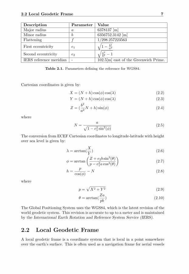
Description Parameter ValueMajor radius a 6378137 [m]Minor radius b 6356752.3142 [m]Flattening f 1/298.257223563First eccentricity e1
√1− b2
a2
Second eccentricity e2
√a2
b2 − 1IERS reference meridian - 102.5[m] east of the Greenwich Prime.
Table 2.1. Parameters defining the reference for WGS84.
Cartesian coordinates is given by:
X = (N + h) cos(φ) cos(λ) (2.2)Y = (N + h) cos(φ) cos(λ) (2.3)
Z = ( b2
a2N + h) sin(φ) (2.4)
where
N = a√1− e2
1 sin2(φ)(2.5)
The conversion from ECEF Cartesian coordinates to longitude-latitude with heightover sea level is given by:
λ = arctan(XY
) (2.6)
φ = arctan(Z + e2b sin3(θ)p− e2
1a cos3(θ)
)(2.7)
h = p
cos(φ) −N (2.8)
where
p =√X2 + Y 2 (2.9)
θ = arctan(Zapb
) (2.10)
The Global Positioning System uses the WGS84, which is the latest revision of theworld geodetic system. This revision is accurate to up to a meter and is maintainedby the International Earth Rotation and Reference System Service (IERS).
2.2 Local Geodetic FrameA local geodetic frame is a coordinate system that is local in a point somewhereover the earth’s surface. This is often used as a navigation frame for aerial vessels

8 Coordinate systems
Figure 2.2. The ENU-frame relative to ECEF coordinate system.
and is fixed in the vessels center of mass. Two axes make up a tangential plane tothe surface of the earth and the third axis is orthogonal to this plane. There aretwo commonly used local frames:
ENU - East,North,Up
NED - North,East,Down
These are both right-handed and the choice of frame depends on the application.The north component in this frame points to the geographical north pole, which isdefined by the earth’s rotational axis, rather than the magnetic north pole which isdefined by the magnetic field generated by the earth’s core. These two differs fromeach other and the magnetic north pole is not constant with time. The down/upcomponent is aligned with the earth’s gravity field and the east component isdefined as east relative to the geographical north pole.
In aviation it is preferred to use a NED-frame due to the fact that positivenumbers are defined down. The ENU-frame can be seen in Figure 2.2 and theNED frame is equivalently constructed.
2.2.1 Velocity relations to WGS
If different coordinate systems are to be used for position, WGS, and velocity,NED, the propagation of the position with respect to NED velocities must be

2.3 Body frame 9
Figure 2.3. The body fixed coordinate system with the rotations defined as φ aroundthe x-axis, θ around the y-axis and ψ around the z-axis.
utilized in the state dynamics. These relationships are given by
λ = VE(Rp + h) cosφ (2.11)
φ = VNRm + h
(2.12)
where Rp and Rm are given by
Rp = a
(1− ε21 sin2 φ)1/2 ≈ a (2.13)
Rm = a(1− ε21)(1− ε21 sin2 φ)3/2 ≈ a. (2.14)
2.3 Body frameThe body frame is fixed to the aircraft’s center of mass where the axes are definedas follow:
x - Straight forward through the nose of the plane.
y - Right of the plane.
z - Down of the plane.
In avionics rotations around these axes are called yaw, pitch and roll. An overviewof the body frame can be seen in Figure 2.3. The angles themselves define theaircraft’s orientation with respect to a local geodetic frame whilst the rotationrates define the aircraft’s motion.

10 Coordinate systems
2.4 Rotation between framesIn a navigation systems, GPS, magnetometers, accelerometers, gyroscopes andpitot tubes are standard sensors. The goal is to estimate position, attitude andheading but the measurements and estimates are in different coordinate systems.To be able to fuse the measurements in a proper manner there must be a mathe-matical connection between measurements and states to be estimated in differentframes. Therefore, some measurements or states must be rotated into anotherframe. Mainly, there are rotations between the body frame and the NED-frame.
There are three common methods to accomplish these rotations:
Euler angles - When using Euler angles to rotate between frames, three separaterotations around single axes are performed. This is an intuitive way ofrotating between frames but is singular when pitch is 90 degrees.
Direction cosine matrix - When using Direction cosine matrix the rotationfrom one frame into another is performed with a single matrix multiplication.This method has no singularities but nine values to keep track of.
Quaternions - When using quaternions to rotate between frames, a single ro-tation is performed around an imaginary vector. This method has no sin-gularities and only four states which is fewer than Direction cosine matrix.The main disadvantage is that there is no intuitive way of interpreting thequaternions.
2.4.1 Euler anglesThe Euler angles are coupled to the notations used in the description of the bodyframe and the NED-frame. These angles themselves represents the attitude of theplane. The Euler angles will be explained using the following notations.
Yaw, (ψ) - The yaw angle is the rotation around the body frame’s z-axis. Theangular difference between the body’s x-axis and the N -axis in the NEDframe is called heading.
Pitch, (θ) - The pitch angle is the angle between the body’s x-axis and the planerepresented by N and E axes in the NED frame.
Roll, (φ) - The roll angle is the rotation around the body’s x-axis. If the planeis flying straight forward but upside down, the roll angle is 180 degrees.
An illustration of the Euler angles can be seen in Figure 2.4.Euler angles are used to describe how a body is oriented with respect to another
frame. When rotating a right handed coordinate system using Euler angles, threesuccessive rotations are done, one on each axis. This can be achieved by:
• Rotate ψ degrees around the body’s z-axis.
• Rotate θ degrees around the body’s y-axis.

2.4 Rotation between frames 11
x
y
- z
ψ
θ
X
φ
z
Figure 2.4. The Euler angles for a rotation between a body frame and the NED frame.
• Rotate φ degrees around the body’s x-axis.
These rotations can be represented as three different rotation matrices [21, 17] asstated in equations (2.15-2.17)
Cψ =
cosψ sinψ 0− sinψ cosψ 0
0 0 1
(2.15)
Cθ =
cos θ 0 − sin θ0 1 0
sin θ 0 cos θ
(2.16)
Cφ =
1 0 00 cosφ sinφ0 − sinφ cosφ
(2.17)
These separate rotations can be put together into one rotation matrix. A rotationfrom the NED frame into the body frame can then be described as
Cbn = CψCθCφ (2.18)
where the notation with subscript n and superscript b means from NED-frame tobody-frame. If (2.18) is calculated using equations (2.15)-(2.17) we get a rotation

12 Coordinate systems
matrix according to:
Cbn =
cos θ cosψ cos θ sinψ − sin θ
sinφ sin θ cosψ− cosφ sinψ
sinφ sin θ sinψ+ cosφ cosψ sinφ cos θ
cosφ sin θ cosψ+ sinφ sinψ
cosφ sin θ sinψ− sinφ sinψ cosφ cos θ
. (2.19)
The fact that,
det(Cψ) = det(Cθ) = det(Cφ) = 1Cψ = CTψ
Cθ = CTθ
Cφ = CTφ
implicates that the rotation matrix is orthonormal as well. The rotation from thebody frame into the NED frame is then given by
Cnb = (Cbn)−1 = (Cbn)T . (2.20)
since Cnb is an orthonormal rotation matrix.
Propagation of Euler angles
The Euler angles are continuously updated through integration of the body’s ro-tation rates, ωx, ωy and ωz. The relationship between body rates and Euler anglespropagation are derived in [21] and is given byωxωy
ωz
=
φ00
+ Cφ
0θ0
+ CφCθ
00ψ
. (2.21)
Solving (2.21) for ψ, θ and φ gives the equations
φ = (ωy sinφ+ ωz cosφ) tan θ + ωx (2.22)θ = ωy cos θ − ωz sinφ (2.23)
ψ = (ωy sinφ+ ωz cosφ) 1cos θ . (2.24)
As seen in (2.24) there is a possibility of division by zero, which results in thesingularity mentioned before. In most ground applications and most helicopterapplications this is not an issue. If a car or equivalent has a pitch of 90, singularityin the Euler angle propagation is probably not the biggest problem. But this canbe used in avionics as well, helicopters for example do not usually fly with 90pitch.
2.4 Rotation between frames 13
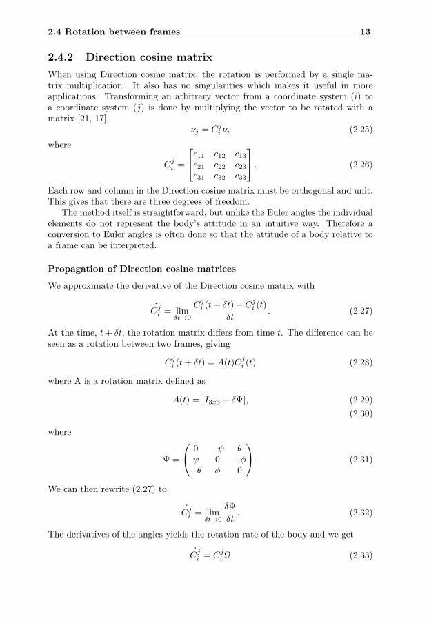
2.4.2 Direction cosine matrixWhen using Direction cosine matrix, the rotation is performed by a single ma-trix multiplication. It also has no singularities which makes it useful in moreapplications. Transforming an arbitrary vector from a coordinate system (i) toa coordinate system (j) is done by multiplying the vector to be rotated with amatrix [21, 17],
νj = Cji νi (2.25)where
Cji =
c11 c12 c13c21 c22 c23c31 c32 c33
. (2.26)
Each row and column in the Direction cosine matrix must be orthogonal and unit.This gives that there are three degrees of freedom.
The method itself is straightforward, but unlike the Euler angles the individualelements do not represent the body’s attitude in an intuitive way. Therefore aconversion to Euler angles is often done so that the attitude of a body relative toa frame can be interpreted.
Propagation of Direction cosine matrices
We approximate the derivative of the Direction cosine matrix with
Cji = limδt→0
Cji (t+ δt)− Cji (t)δt
. (2.27)
At the time, t+ δt, the rotation matrix differs from time t. The difference can beseen as a rotation between two frames, giving
Cji (t+ δt) = A(t)Cji (t) (2.28)
where A is a rotation matrix defined as
A(t) = [I3x3 + δΨ], (2.29)(2.30)
where
Ψ =
0 −ψ θψ 0 −φ−θ φ 0
. (2.31)
We can then rewrite (2.27) to
Cji = limδt→0
δΨδt
. (2.32)
The derivatives of the angles yields the rotation rate of the body and we get
Cji = Cji Ω (2.33)

14 Coordinate systems
where
Ω =
0 −ωz ωyωz 0 −ωx−ωy ωx 0
. (2.34)
The Direction cosine matrix has an advantage over Euler angles due to the factthat it lacks singularities. There are only three degrees of freedom, but there arenine elements to update in every iteration. If a rotation is to be embedded in anExtended Kalman filter this is a big drawback since it is desirable to have as fewstates as possible to reduce complexity.
Relations to Euler angles
When using Euler angles the three consecutive rotations were multiplied togetherto form a single rotation matrix. Since Direction cosine matrix is a rotation per-formed by a single matrix multiplication, this matrix must be equal to the rotationmatrix achieved by using Euler angles according to
Cji,Euler = Cji,DCM. (2.35)
From the Direction cosine matrix we can derive the Euler angles from the rela-tionship
cos θcosψ cos θ sinψ − sin θ
sinφ sin θ cosψ− cosφ sinψ
sinφ sin θ sinψ+ cosφ cosψ sinφ cos θ
cosφ sin θ cosψ+ sinφ sinψ
cosφ sin θ sinψ− sinφ sinψ cosφ cos θ
=
c11 c12 c13c21 c22 c23c31 c32 c33
(2.36)
by comparing the elements and get
φ = arctan(c32
c33
)(2.37)
θ = arcsin (−c31) (2.38)
ψ = arctan(c21
c11
). (2.39)
There exists a singularity at 90 pitch here as well when converting from Directioncosine matrix to Euler angles. In these cases other types of conversions to Eulerangles must be used.
2.4.3 QuaternionsThe theory of quaternions was described by Sir William Rowan in 1843. Theusage of quaternions as a rotation between frames was described by BenjaminOlinde Rodrigues. So the rotation method described in this section is often calledEuler-Rodrigues’ rotation formula. In avionics combined with Kalman filtering,

2.4 Rotation between frames 15
x
y
z
y'
x'
φ
Figure 2.5. Rotation from x, y to x′, y′ is done by rotating φ degrees around z.
this is probably the most common method to rotate between frames. There areno singularities and four states to update, which is fewer than the Direction cosinematrix.
The idea of using quaternions is that we can rotate a three dimensional frameinto another around a vector that is orthogonal to the three dimensional space.This can be exemplified by the rotation of a two dimensional plane. The relation-ship between the two frames, (x, y) and (x′, y′), in Figure 2.5 is a rotation of φdegrees around the z-axis.
A 4-dimensional quaternion is defined as
q = q0 + q1i + q2j + q3k =[q0 q1 q2 q3
] 1ijk
(2.40)
where i, j and k are imaginary components. Multiplication between quaternionimaginary components are similar to ordinary imaginary multiplication. The mul-tiplication rules for quaternions are given by
i · i = −1 i · j = k i · k = −jj · j = −1 j · i = −k j · k = ik · k = −1 k · i = j k · j = −i
. (2.41)
To specify a vector from a body frame, r in a NED frame, the components areredefined as the complex components of a quaternion.
r = ir1 + jr2 + kr3 + 0 (2.42)
where the scalar is set to zero. Then the rotation is defined as [23]
rn = q∗rbq. (2.43)

16 Coordinate systems
q∗ denotes the complex conjugate of q and is defined as a negation of all thecomplex components. For quaternions the complex conjugate is the same as theinverse. The multiplication between two arbitrary quaternions is defined as
q · p =(q0 + q1i + q2j + q3k) · (p0 + p1i + p2j + p3k)=(q0p0 − q1p1 − q2p2 − q3p3) + (q0p1 + q1p0 + q2p3 − q3p2)i
+ (q0p2 − q1p3 + q2p0 + q3 + p1)j + (q0p3 + q1p2 − q2p1 + q3p0)k
=
q0 −q1 −q2 −q3q1 q0 −q3 q2q2 q3 q0 −q1q3 −q2 q1 q0
p0p1p2p3
. (2.44)
Expanding (2.43) according to (2.44) gives the equation:
rn =[0 00 C
]rb (2.45)
C is the rotation matrix, derived in [23], used to rotate a vector between differentframes and is equivalent to the Direction cosine matrix. The difference is whatthe individual elements represents and how they propagate.
C =
q20 + q2
1 − q22 − q2
3 2(q1q2 + q0q3) 2(q1q3 − q0q2)2(q1q2 − q0q3) q2
0 − q21 + q2
2 − q23 2(q2q3 + q0q1
2(q1q3 + q0q2) 2(q2q3 − q0q1) q20 − q2
1 − q22 + q2
3
(2.46)
Propagation of quaternions
The change rate of the quaternion rotation matrix [22] is given by:
q = 0.5q · pbnb (2.47)
where
pbnb =
0ωbxωbyωbz
(2.48)
and ωbi is the rotation rates in the body frame. Expanding this equation accordingto (2.41) gives
q1q2q3q4
= 0.5
q0 −q1 −q2 −q3q1 q0 −q3 q2q2 q3 q0 −q1q3 −q2 q1 q0]
0ωxωyωz
. (2.49)
This can be rewritten as0 −ωx −ωy −ωzωx 0 ωz −ωyωy −ωz 0 ωxωz ωy −ωx 0
q0q1q2q3
=
−q1 −q2 −q3q0 −q3 q2q3 q0 −q1−q2 q1 q0
ωxωyωz
. (2.50)

2.4 Rotation between frames 17
For further use, the following expressions are defined,
q = 12S(ω)q, q = 1
2 S(q)ω (2.51)
where,
S(ω) =
0 −ωx −ωy −ωzωx 0 ωz −ωyωy −ωz 0 ωxωz ωy −ωx 0
(2.52)
S(q) =
−q1 −q2 −q3q0 −q3 q2q3 q0 −q1−q2 q1 q0
. (2.53)


Chapter 3
Sensors
The sensors on EasyPilot belong to the MEMS technology. MEMS stands forMicro-Electro-Mechanical Systems, and it consists of extremely small sensor ele-ments between 0.02[mm] and 1[mm] together with a processing unit. This typeof sensor is common in a strapdown system, where all the sensors are fixed on achip. This is also the case for EasyPilot.
3.1 GyroscopesMEMS gyroscopes measures rotation rate around fixed axes. These are used invarious applications due to their low cost. The autopilot is equipped with a 3-axis analog MEMS gyroscope which measures the roll-rate, pitch-rate and yaw-rate. Gyroscopes are useful from many aspects, they can be integrated to acquireorientation or the rotation rates can be used to suppress external disturbances.The analog sensors are sampled by the processor at approximately 200Hz. Whenlogging from the autopilot, limitations in transfer rates set the sample rate to120Hz. The gyroscopes bandwidth is higher than this and therefore the Nyquistcriteria is not fulfilled, thus yielding limitations in frequency analysis.
3.1.1 PerformanceThere are several factors to consider when evaluating a gyroscope [1], such asScale factors - Since it is an analog sensor the measured voltage from the sensor
must be scaled to rotation rate. This number is often given by the man-ufacturer, but it may vary between components. This factor can also bedependent on temperatures and accelerations.
Non-linearity of scale factors - The scaling factor is not necessarily a constant,it may differ between different rotation rates.
Alignment errors - The axes of the sensor can be non-orthogonal. This meansthat if we rotate the sensor around one of its axes, another axis will sensethe rotation as well.
19

20 Sensors
Bias - If the sensor is laying still and if it has not got zero mean on all axes, abias is present.
Bias and scaling stability - The bias and scaling factor are not always constantover time.
Random drift rate - The noise on the sensor output is often analyzed in termsof Allan variance [2, 25]. This is however not presented here due to the factthat the bandwidth of the gyroscopes is higher than the sample rate, whichmeans that the Nyquist criteria is not fulfilled.
These types of errors can be compensated for by calibration. But there are otherperformance factors that are sensor specific such as resolution, bandwidth, turn-on time and shock resistance. To get a good calibration that takes all errors intoaccount, reliable measurement equipment is needed. During this master thesis nosuch equipment is available. Because of this, the only errors that will be calibratedfor are bias and a constant scaling factor. The change in bias that may occur willbe handled by filtering and is described in Chapter 4 and 5.
3.1.2 Statistical analysisMost information about the gyroscopes can be gathered by collecting data whenthe sensor is placed at stand-still. In this section bias and noise levels will beanalyzed and compared to the sensor datasheet.
In Figure 3.1, measurements from the 3-axis gyroscope is plotted. From thisdataset we can derive bias and variance. Due to limitations in communication thegyroscopes are sampled at approximately 120Hz. The bias is computed simplyby taking the mean of each sensor. The biases for the gyroscopes are presented inthe table below.
Gyroscope Bias [rad/s]Roll −0.1069Pitch −0.1268Yaw −0.0192
The typical rate noise density of the gyroscopes from the datasheet is givenin /s/
√Hz. These are calculated from the same dataset as the biases above.
The rate noise density and variance for the gyroscopes used are given in the tablebelow.
Gyroscope Rate noise density [/s/√Hz] Variance [rad2/s2]
According to manufacturer 0.035 –Roll 0.0873 2.84e− 4Pitch 0.1231 5.65e− 4Yaw 0.0390 5.66e− 5

3.1 Gyroscopes 21
0 1 2 3 4 5 6 7 8−0.2
−0.1
0Static gyroscope measurements
0 1 2 3 4 5 6 7 8−0.2
−0.1
0
[rad
/ s]
0 1 2 3 4 5 6 7 8−0.05
0
0.05
time[s]
Figure 3.1. Gyrscope measurements in [rad/s] from all three gyros, roll, pitch and yaw.
Even though the noise rate densities from the measurements are higher thanthe typical rate noise density from the datasheet, this is not interpreted as a mal-functioning gyroscope. The typical values are given assuming that the gyroscopeis mounted at an ideal position, that the input voltage is good and that thereare no external disturbances. The EasyPilot is however not an ideal mountingposition since there are a lot of components causing local disturbances in powersupply and inducing currents in the gyroscope circuit.
3.1.3 CalibrationThe gyroscopes are calibrated for bias and scaling. The output voltage, U fromthe gyroscope is translated to an angular rate according to
ω = (U − bU ) · k (3.1)
where bU is the bias in voltage and k is the scaling factor. The bias factor can beidentified by sampling the gyroscopes when they are lying still with good precision.To get a good calibration on the scaling factor, a precise known rotation is neededaround a single axis. When using the gyroscopes together with a filter that usesaccelerometer and magnetometer, the scaling factor is not crucial. If a rotationof 90 is performed and the gyroscope is integrated to 85, the accelerometer andmagnetometer will cause the orientation to converge to its correct value. Thisis described in Chapter 5. In this case the calibration algorithm proposed inAlgorithm 1 may be sufficient.

22 Sensors
Algorithm 1 Gyroscope calibration
1. Sample the gyroscope when it is lying still
2. Calculate bias:
For measurement mi, i = 1,2,...,M,
bU = 1M
∑Mi=1 mi
3. Set kold = 1
4. Sample the gyroscope when rotating 360 degrees around its axis
5. Calculate the scaling:
For measurement mi, i= 1,2,...,M, and sampling time Ts
knew = 2π/(Tskold
∑Mi=1 mi
)6. Set kold = knew · kold Repeat from (4) until knew = 1.
7. Repeat from (1) for all gyroscope axes.

3.2 Accelerometer 23
3.2 AccelerometerAn accelerometer measures proper acceleration, that is weight per unit of a testmass. This means that the actual gravity of the earth is measured as well asaccelerations due to motion. Since the gravity vector is known, the accelerometercan be used to estimate both orientation and acceleration. It is however impossibleto distinguish acceleration from orientation if neither is known. The accelerometerused in EasyPilot is an analog 3-axis MEMS accelerometer.
3.2.1 PerformanceThe performance of an accelerometer can be evaluated in roughly the same way asthe gyroscopes. They are both of MEMS technology and will therefore have thesame errors related to MEMS construction. While the accelerometer can be usedto gain long-term stability in orientation, it will only have short term stability innavigation since the position is a double integration. This can be illustrated bysolving the following integral,
v =t∫
0
a(t) + bdt =t∫
0
a(t) dt+ bt (3.2)
where the integral over a(t) is the true velocity and bt is the integrated bias error.A second integral solving the position will cause the bias error to be even larger.And over time, the term bt will be very significant.
More performance criteria and how to measure them are described in Chapter8 in [21]
3.2.2 Statistical analysisIn Figure 3.2 the accelerometer is sampled at 120Hz at stand-still flat oriented,which means that the z-axis accelerometer should measure one negative g in meanand the x- and y-axis should have zero mean. The bias on the x- and y-axis can bederived by just taking the mean of the measurements. The z-axis accelerometermeasures the gravity vector which needs to be taken into account. The bias of thez-axis for N measurements, mz, becomes
bz = 1N
N∑k=1
(mz + g). (3.3)
In the table below the accelerometer biases are presented.
Accelerometer [g]x-axis −0.0475y-axis 0.0562z-axis −0.0406

24 Sensors
0 1 2 3 4 5 6 7 8−0.06
−0.04
−0.02Static accelerometer measurements
0 1 2 3 4 5 6 7 80.04
0.06
0.08
[g]
0 1 2 3 4 5 6 7 8−1.1
−1
−0.9
time[s]
Figure 3.2. Accelerometers measuring acceleration in unit [g]. From top, x-axis, y-axisand z-axis. The accelerometer is laying flat and is not calibrated.
When performing measurements for estimation of accelerometer bias the ori-entation of the sensor is of importance. If the sensor is tilted some degrees thex- or y-axis sensors will measure a small part of the gravity. This must not beinterpreted as a sensor bias.
The noise performance on the sensor is given by the manufacturer is µg/√Hz.
From the dataset presented in Figure 3.2, the mean is removed and noise densityis calculated. The noise ratios of the sensor together with typical values frommanufacturer are presented in the table below.
Accelerometer Noise density µg/√Hz Manufacturer typical value µg/
√Hz
x-axis 193.92 150y-axis 207.62 150z-axis 454.60 300
Here, the noise ratios are higher than the manufacturers typical values. Since thegyroscopes showed the same result this is probably due to external disturbancesas discussed in Section 3.1.2.
3.2.3 CalibrationSome of the errors in the sensor can be calibrated for. In this report a calibrationalgorithm that is compensating for scaling errors and bias in the individual axes

3.3 Magnetometer 25
Figure 3.3. An illustration of the accelerometer calibration as given in Algorithm 2.
are presented in Algorithm 2. An illustration of the calibration algorithm can beseen in Figure 3.3.
Algorithm 2 Accelerometer calibration
1. Collect M1 samples m1,i of accelerometer with an axisaligned with the direction of gravity
2. Collect M2 samples m2,i of accelerometer with the sameaxis aligned with the opposite direction of gravity
3. Calculate the off-set ba according to
ba = 12
(1M1
∑M1i=1 m1,i + 1
M2
∑M2i=1 m2,i
)4. Calculate the scaling factor according to
k = 1/(
1M1
∑M1i=1 m1,i − ba
)5. Repeat from step (1) on all accelerometer axes.
Sometimes the accelerometer axes may be misaligned, non-orthogonal. If themisalignment is significant, or if it is of great importance that no misalignmentexists, this can also be calibrated for. An algorithm for this is presented in [19].
3.3 MagnetometerIn avionics a magnetometer is often used to calculate heading of the vessel. Theheading can be calculated by measuring the strength and direction of the magnetic

26 Sensors
Figure 3.4. A 2D projection of the earth’s magnetic field.
field since the earth’s magnetic field is known. The field strength is measured inWeber per square meter (Wb/m2), which is the same as Tesla (T ), or in Gauss(G) where,
1[G] = 0.0001[T ]. (3.4)The earth’s magnetic field, even though it is known, is very small (from 0.3Gin South Africa to 0.6G near the poles). This means that the sensor will be verysensitive to disturbance fields, such as electric motors, high voltage wires, hard ironmaterials etc. The earth’s magnetic field can be seen in a 2D projection in Figure3.4. Here it can be seen that the angle between the surface and the magnetic fieldincreases as we get closer to the magnetic poles, this is called inclination or dip.The same Figure also illustrates the deviation between the geographic north andmagnetic north. The angle between magnetic north component and the geographicis called the declination. In Linköping the declination is approximately 4 degreesand the inclination 70 degrees. This will result in larger uncertainties in headingestimation since the magnetic component in the horizontal plane is small relativeto the component in the vertical plane.
The EasyPilot is equipped with a tri-axis anisotropic magnetoresistive (AMR)magnetometer. This type of magnetometer is very small and is often used instrapdown applications. In the NED frame the earth’s magnetic field can beseparated into three components. In Linkping these are given by
Component ValueNorth 15.741 [µT]East 1.1304 [µT]Down 48.422 [µT]
In the NED frame this will look like in Figure 3.5. The magnetometer itselfwill measure a rotation of this vector depending on its orientation.

3.3 Magnetometer 27
N
E
D
Earth Magnetic field vector
Figure 3.5. The earth’s magnetic field in Linköping relative to a NED frame.
R+δR
R+δR
R-δR
R-δR
δVmeas V
II
Earth magnetic field
Figure 3.6. Illustration of one of the three wheatstone bridges in an AMR magnetome-ter.
3.3.1 Anisotropic Magnetoresistive elementsThe AMR sensor is constructed by three orthogonally placed magnetic field sen-sors. Each sensor consists of four magnetoresistive elements that are mounted ina square, a so-called wheatstone bridge. A voltage is applied over two oppositecorners of the square and the output voltage is measured over the two others, seeFigure 3.6. That means that the measured output should be half of the appliedvoltage. Due to magnetic interference from external magnetic fields the resistanceof the elements in the wheatstone bridge will change, thus changing the outputvoltage. This change in output voltage is used to calculate the magnetic fieldstrength [16]. In a tri-axis AMR there are three orthogonally placed wheatstonebridges which allow the sensor to sense a magnetic field in three dimensions.
3.3.2 Measurement errorsThere are two types of errors that have to be considered to be able to get goodreadings from the sensors, manufacturing errors and environmental errors. Some

28 Sensors
of these are constant for each sensor and some vary for different environments. Thenext section will describe how these effects are being accounted for. The effectsmentioned below are thoroughly described in [16].
Wheatstone bridge alignment errors
When calculating the magnetic field we use the fact that the output voltage fromthe wheatstone bridge is half of the applied voltage. When an external magneticfield is applied the resistance in the circuit will change. But to get an expectedreading of the output voltages from the tri-axis AMR it is required that the wheat-stone bridges are exactly orthogonal to each other. Due to manufacturing errors,they are not. This misalignment is constant and sensor specific and does not varyover time.
Element sensitivity errors
The elements in the AMR are not linear in respect to applied magnetic field. Acalibration in an environment where the magnetic field strength is 0.6G is notvalid in an environment where it is 0.4G. But since the sensor are to be usedin a known environment there is only a scale factor between output voltage andmagnetic field. This scale factor would not be valid if the AMR is put in a differentenvironment where the strength of the magnetic field is not the same for whichthe scale factor was derived.
Element magnetization errors
Over time the elements in the AMR will be magnetized. This will result in achange of the sensor’s sensitivity axis. This effect is often referred to as cross axissensitivity errors. If the environment provides a constant magnetic field the normof the measured magnetic field would be constant. But when the sensitivity axis ofthe individual elements of the wheatstone bridge differs, this will not be the case.This will result in an illusion that the magnetic field strength of the surroundingschange due to the magnetometers orientation.
Hard iron errors
Hard iron errors have nothing to do with the sensor itself, but rather the platformit is mounted on. Hard iron effects are defined by a magnetic source with aconstant magnetic field, independent of the platform’s orientation. This will causea perturbation of the magnetic field which will manifest itself as a bias in thesensor readings. An example of this is if the magnetometer is mounted near a wiredelivering current. The wire’s orientation relative to the magnetometer will neverchange which means that the disturbance caused by it will be constant.
Soft iron errors
Soft iron deviations are of a more complex nature. These are caused by ferromag-netic materials that are excited by the earth’s magnetic field. Because of this, the
3.3 Magnetometer 29
magnetic field disturbance will change with the platforms orientation.
3.3.3 CalibrationWhen calibrating the magnetometer a compensation for all the effects describedin Section 3.3.2 will be done. Due to the hard and soft iron errors the calibrationmust be done when the sensor is mounted on the desired platform. A measurementmodel including all the errors that are to be compensated for is derived, then aleast squares method [11] is used to estimate the parameters.
Measurement model
If only measurement errors are taken into account the model would look like
h = hs + ε (3.5)
where
h− Measured magnetic fieldhs − Sensor indicated magnetic fieldε−Measurement noise
The sensor indicated magnetic field is however not the same as the earth magneticfield. The hard iron effects can be compensated with a bias term according to,
bhi = [bhix bhix bhix ]T . (3.6)
The effects of soft iron changes the direction of and strength of the sensed field inrespect to how the platform is oriented relative to the earth’s magnetic field. Thiseffect can be modeled by a scaling of the true field with a 3 by 3 matrix,
Asi =
a11 a12 a13a21 a22 a23a31 a32 a33
(3.7)
This means that the field that the sensor is actually measuring is
h = Asi(he − bhi) (3.8)
What is left is to compensate for the measurement errors in the actual sensor. Asdepicted in Section 3.3.2, we must compensate for the wheatstone bridge misalign-ments and the scaling of the current magnetic field. The misalignments are com-pensated for by multiplying the measurement with a 3 by 3 matrix that projectsthe measurements on the orthogonal frame on which the sensor is mounted. Thescaling of the current magnetic field is compensated for by multiplying the mea-surements with a 3 by 3 diagonal matrix and the bias is subtracted from the

30 Sensors
measurement. The following compensation factors are introduced:
M =
m11 m12 m13m21 m22 m23m31 m32 m33
non-orthogonality compensation
S =
s11 0 00 s22 00 0 s33
scaling compensation
bs = [bsx bsx bsx ]T sensor bias compensation
This yields the measurement equation
h = SM(Asihe + bhi) + bs + ε (3.9)
where h is the measured field and he is the earth’s magnetic field in the frameof the sensor and ε is noise. Although there are a lot of factors affecting themeasurement we are not interested in the individual contributions from specificerrors, thus introducing:
h = Ahe + b + ε (3.10)where,
A = SMAsi (3.11)b = SMbhi + bs. (3.12)
Here, A represents all the scalings and rotations and b all the biases.To be able to calculate a vessels orientation we want to know in which direction
the earth magnetic field is oriented with respect to the frame of the vessel. Fromequation (4.28) we can derive the earth magnetic field in the frame that the sensoris mounted,
h = A−1(h− b−ε) (3.13)
3.3.4 Calibration algorithm using least squaresEquation (3.13) cannot be solved directly using least squares since it is not inquadratic form. But h is the earth’s magnetic field in the frame of the sensor, andunder the assumption that the magnitude of the earth’s magnetic field is constantthe following equation is given:
H2m − hTh = 0 (3.14)
where Hm is the magnitude of the earth’s magnetic field. Substituting h in equa-tion (3.14) with (3.13) yields the equation
(h− b)T(A−1)TA−1(h− b)−H2m = 0 (3.15)
which can be expanded to
h(A−1)TA−1h− 2(A−1)TA−1bh + bT(A−1)TA−1b−H2m = 0. (3.16)

3.3 Magnetometer 31
This is a quadratic equation according to
hTQh + uTh + k = 0 (3.17)
where
Q = (A−1)TA−1 (3.18)u = −2Qtb (3.19)k = bTQb−H2
m (3.20)
Q is symmetric due to its definition. Thus we can rewrite (3.17) to obtain,
0 = yTβ (3.21)
where
yT =[(h⊗ h)T hT 1
](3.22)
β = [Q11 Q12 Q13 Q22 Q23 Q33 u1 u2 u3 k]T (3.23)
where ⊗ is the kronecker product. The least squares cost function is definedaccording to
qls(β; h) = (yTβ)2 = βTyyTβ (3.24)
qls is associated with the cost for one measurement. For solving the least squareproblem we formulate
Qls =m∑l
βTy(l)y(l)Tβ = βTΦβ (3.25)
where y(l) is associated with the l’th measurement. There are several ways ofsolving the least squares problem defined in (3.25). Here, (3.25) is minimized bysetting β⊥νi, where νi is the eigenvector associated with the smallest eigenvalueof Φ. β is given by the normalized eigenvector:
β = νi|νi|
(3.26)
Q, u and k can now be reconstructed from β, where the lower triangular of Q isset to the upper triangular of Q. The bias term in (3.13) is solved directly by,
b = −12Q−1u. (3.27)
To acquire A−1 from (3.13), equation (3.18) can be solved using Cholesky de-composition, giving the complete solution for the magnetometer projection on asphere,
h = A−1(h− b). (3.28)

32 Sensors
−0.5
0
0.5
1−0.5 0 0.5 1
−1
−0.5
0
0.5
1
−1
0
1−0.5 0 0.5 1
−1
−0.8
−0.6
−0.4
−0.2
0
0.2
0.4
0.6
0.8
1
Figure 3.7. To the left is the non-calibrated data with normalized amplitude. To theright is the same data but calibrated.
3.3.5 Calibration resultsWhen calibrating the magnetometer the sensor must be mounted in the samesettings as when it is to be used. The magnetometer is fixed to EasyPilot and theEasyPilot is mounted in the aircraft Spy Owl 100. The plane is moved aroundto collect measurements in various orientations. As seen in the left plot in Figure3.7, the magnetometer is in need of calibration. In the right plot the same data iscalibrated and plotted against the same reference sphere.
3.4 Pressure sensorsIn most avionic applications, pressure sensors are used. EasyPilot is equipped withtwo analog MEMS pressure sensors, one to measure the static pressure and oneto measure the stagnation pressure. Stagnation pressure is defined by Bernoulli’sequation
stagnation pressure = static pressure + dynamic pressure. (3.29)
In Figure 3.8 a static source, measuring static pressure, and a pitot tube, measuringstagnation pressure are illustrated for a vessel in motion. When in motion, theair molecules will enter the pitot tubes and press against the inner wall. This willincrease the density of air molecules in the pitot tube. But due to the second lawof thermodynamics the density will only increase to a certain point, equilibrium.Depending on the speed of the vessel, this equilibrium will correspond to differentdensities of air in the pitot tube. The stagnation pressure is the pressure measuredinside this tube.
The static source is used to measure the pressure surrounding the vessel and thedifference between static pressure and stagnation pressure gives dynamic pressure.

3.4 Pressure sensors 33
Figure 3.8. The static source (upper) measures static pressure, the pitot tube (lower)measures stagnation pressure. The dots illustrate the density of air molecules.
Knowing the pressure at ground level the height of the vessel can be derived fromthe static pressure and knowing the dynamic pressure the air speed can be derived.This derivations are described in Section 4.2.5.
3.4.1 Performance
The pressure sensors used are MEMS technology and will have noise and bias.The difference between gyroscopes, accelerometers and magnetometers is that wedo not have a constant reference to determine bias from. To be able to biascompensate we must know the exact pressure in the room where we analyse it.But since the air pressure is not constant, the more attractive option is to calibratean offset, in which the bias is included.
One performance factor that can vary between manufacturers, that is impor-tant in Sweden, is the temperature operation interval. Some manufacturers sup-port down to −40C and some support only down to 0C.
3.4.2 Calibration
When the aircraft is standing still on the ground, the stagnation pressure andstatic pressure should both be the same. In this calibration it is assumed that theground pressure is equal to the standard atmospheric pressure, 101.325[kPa]. Thecalibration of the pressure sensors will therefore only include a bias compensation.The main focus of this calibration is to make sure that the stagnation pressureand static pressure is the same when the aircraft is not moving. If they are not, afalse indication of air speed will be persistent.

34 Sensors
3.5 GNSSGNSS, or Global Navigation Satellite System, is a navigation system based onsatellites with global coverage such as GPS, GLONASS and soon to be operatingGalileo. All satellites within a GNSS have synchronized clocks and transmit theirclock time regularly. A receiver compares time of arrival from several differentsatellites and from this information position can be derived. The American GNSS,GPS, was the first GNSS system to become available for civil use in 1983. At thispoint there were still restrictions for the civil market which were removed in 2000.
There are a lot of receiver manufacturers on the market that treat the signalsfrom the satellites in their own way and they also choose what data to deliver. Themanufacturers usually support most of the data specified in the protocol specifiedby National marine electronics association, NMEA, as given in [18]. When usinga GNSS in a product the user must rather choose from the variety of settingsthe manufacturer provides rather than calibrate it. The most common receiversettings and how they affect performance are thoroughly described in [12].
3.5.1 Position estimationIf the receiver clock is synchronized with the satellite clock and the satellite clockemits its current time, the distance from the satellite can be calculated. This isbecause it will take time for the satellites clock pulse to reach the receiver. Thedifference in time of arrival and the emitted time stamp can be used to calculatethe distance to the satellite according to
d = c∆t (3.30)
where ∆t is the difference between time of emitting and time of arrival. In a 2Dexample this means that the receiver must be located on the circle with radius d,3.9. Since we know that we must be located on the earth (on the circumference ofthe 2D circle) there are only two possible positions to be at, see Figure 3.9. In thesame Figure another satellite is added, which eliminates one of the possibilities,thus yielding the true position of the receiver.
In the real world we have three dimensions, which means that we must addone extra satellite to be able to determine a position. Also, the satellites havesynchronized atomic clocks which the receiver has not. The unknown time bringsan extra dimension in to the problem and therefore four satellites are required todetermine the position in a GNSS [27].
3.5.2 Speed and direction estimationAlthough many receivers use extensive filtering from positioning to acquire speed,modern devices may also track the frequencies of the satellite signals and estimatespeed using the Doppler effect [5]. The Doppler effect is illustrated in Figure 3.10.This principle is based on the experienced wavelength of GPS signals. If a receiveris moving towards a satellite, the wavelength will be experienced as shorter thanif the receiver was moving away from it.

3.5 GNSS 35
Figure 3.9. Illustration of GNSS positioning principle in 2D.
Figure 3.10. The principle of determining speed using the Doppler effect. When theplane moves away from the satellites the experienced frequency of the GPS signal seemslower than if it is moving towards it.


Chapter 4
Modelling
In systems like the autopilot, the measurements given by the sensors themselvesare not what is interesting. In most cases we want to know information about thesystem that has sensors mounted on it. If we want to know how a plane is sideslipping in the wind, there is no sensor to measure this. Therefore, we must relatewhat we can measure to what we want to know.
A measurement model is a mathematical description of what is being measured.This can be exemplified by a gyroscope that measures rotation rate in [rad/s]. Asimple measurement model relating the measurement to [/s] can then be statedas
y = π
180θ (4.1)
where y is the measurement given in [rad/s] by the gyroscope and θ is rotationrate given in [/s].
Virtual measurements can also be created in a similar way. If it is required tohave a measurement in [/s], equation (4.1) can be arranged to
y′ = 180yπ
. (4.2)
This type of manipulation of measurement equation is a simple way of extractinginformation. It can however cause problems since we will always manipulate thenoise of the sensors as well. In reality, what is being measured by the gyroscope is
y = π
180θ + v (4.3)
where v is measurement noise. When the measurement equation is rearranged,the true result becomes
y′ = 180π
( π
180θ + v)
= θ + 180θv. (4.4)
Filters like the Extended Kalman filter do not require manipulation of themeasurement equations. The measurement equation is derived so that the mea-surement is a function of states included in the filter. This gives the possibility to
37

38 Modelling
add measurements that measures a mixture of states. For example, if a sensor ismeasuring wind speed a simple measurement equation could look like
y = vground + vwind. (4.5)
If vground and vwind are included as states in an Extended Kalman filter, thismeasurement can be used as a measurement equation without manipulation.
In the Extended Kalman filter case a model over the system is derived accordingto
x = f(x) (4.6)y = g(x) + v. (4.7)
Here, x is the state of the Extended Kalman filter, f is the function describ-ing the system dynamics, y is the measurements, g is the equation relating themeasurements to the system states and v is the measurement noise.
Each section in this chapter describes required models for a certain type offilter. First system models are presented to give an overview of what is to beestimated. Then the measurement models or virtual measurements that relatesthe system models to the measurements are presented.
4.1 Height estimation modelThe height can be described as a function of pressure, and is derived in [26],
h = K log(Ps0
Ps
)+ h0 (4.8)
where h0 is the height at ground level, Ps0 is the static pressure at ground leveland K is a parameter that depends on temperature.
We can rearrange (4.8) to acquire
h− h0 = K (log(Ps0)− log(Ps)) =[1 − logPs
] [K log(Ps0)K
](4.9)
We now have an equation on the form
y = ψT θ (4.10)
where
ψ =[
1− log(Ps)
], θ =
[K log(Ps0)
K
]. (4.11)
This model is derived under the assumption that the current pressure, Ps, is aknown parameter. The model proposed here is designed so that a parameterestimation using RLS, Recursive Least Squares, with exponential forgetting factorcan be utilized to estimate K in real-time. The RLS algorithm is described in

4.2 INS state space models 39
Section 5.2 The drawback with this method is that the pressure at ground levelcan change, for example due to an incoming low pressure area.
The reason this model is proposed for use together with RLS is due to thedifficulty of performing a calibration, providing K and Ps0. It is more appropriateutilizing information from the GPS to estimate K in real-time, after Ps0 and h0has been set as constants at ground.
4.2 INS state space models
An INS, Inertial Navigation System, is a system that calculates position, velocityand orientation. With the given sensors for EasyPilot, the following four modelsare presented with no input signals. The position is defined in Longitude-Latitude,the velocities and accelerations are described in the NED frame and the quater-nions represent a rotation from a body frame to the NED frame.
The models proposed only includes kinematic relationships between states dueto the fact that the autopilot is to be used in many different air frames. If theautopilot where to be used in a specific airframe, a model over the system couldhave been derived. This would of course result in higher complexity, but mostlikely you could expect better performance.
Model 1
The states we want to estimate is the position, p, velocities, v, and the orien-tation, q. The sensors that we want to utilize are gyroscopes, accelerometers,magnetometers and GPS. If we want to use the accelerometer, which measures thegravity vector as well as acceleration, we must include states for acceleration. Theaccelerometer also has biases, which is why we must add states for this as well.The gyroscopes measures change in orientation which can be used as an input, oras in this case, added as states. The gyroscopes will also measure a bias whichmust be included as separate states. The GPS measures velocities and the magne-tometer measures the magnetic field. Other effects that these sensors might haveare disregarded. It is important to decide what effects to include in a state spacemodel to make the best use of available sensors. For example, the magnetometerhas bias to and the accelerometers and gyroscopes has scaling factors that mayvary. But if to many effects are added, without additional sensors, the model willbe non observable.
40 Modelling
This model can be studied further in [8] and is given by:
pvaqω
bacc
bgyro
=
0 P (p) 0 0 0 0 00 0 I 0 0 0 00 0 0 0 0 0 00 0 0 0 S(ω)/2 0 00 0 0 0 0 0 00 0 0 0 0 0 00 0 0 0 0 0 0
pvaqω
bacc
bgyro
+
0 0 0 00 0 0 0I 0 0 00 0 0 00 I 0 00 0 I 00 0 0 I
va
vω
vb,a
vb,ω.
(4.12)
S(ω) is defined in (2.52) and P (p) is the relationship between NED velocitiesand position given by WGS84 as defined in (2.11) and (2.12). These are non-linear functions, and this is therefore not a proper state space model. To make anapproximation of a state space model, S(ω) and P (p) must be linearized. Thiscan be seen in Appendix A.
Model 2
The second proposed model includes all states as Model 1 to make use of gy-roscopes, accelerometers, magnetometer and GPS. In addition to these sensors,measurements from pitot tubes are to be added. The pitot tube measures the sumof airspeed and ground speed, hence we must add states for the wind to allow thismeasurement.
Model 1 is augmented with the following states,
w =(wNwE
)(4.13)
where the wind has a strength defined in north and east respectively. The second

4.2 INS state space models 41
model is then formed according to:
pvaqω
bacc
bgyro
w
=
0 P (p) 0 0 0 0 0 00 0 I 0 0 0 0 00 0 0 0 0 0 0 00 0 0 0 S(ω)/2 0 0 00 0 0 0 0 0 0 00 0 0 0 0 0 0 00 0 0 0 0 0 0 00 0 0 0 0 0 0 0
pvaqω
bacc
bgyro
w
+
0 0 0 0 00 0 0 0 0I 0 0 0 00 0 0 0 00 I 0 0 00 0 I 0 00 0 0 I 00 0 0 0 I
va
vω
vb,a
vb,ω
vw
(4.14)
Model 3
A simpler model can be stated if only the orientation of the plane is of interest.This model can use gyroscope, magnetometer and accelerometer as measurements.
aqω
bgyro
=
0 0 0 00 0 S(ω)/2 00 0 0 00 0 0 0
aqω
bgyro
+
I 0 00 0 00 I 00 0 I
va
vω
vb,ω
(4.15)
This model includes 13 states which reduces the complexity when applying anExtended Kalman filter to it. Information that would be useful for estimatingacceleration in the body is lost. For this model to work a good and reliablemagnetometer and a well calibrated accelerometer is a must.
Model 4
Another simple model that only holds states for position, speed, heading and windspeed can be formed according to:
pvwθ
=
0 P (p) 0 00 0 0 00 0 0 00 0 0 0
pvwθ
+
0 0 0I 0 00 I 00 0 1
vvvwvθ
(4.16)
where θ is the heading of the plane.Usage of this model demands a GPS, pitot tubes and magnetometer. The
magnetometer is used to calculate an artificial measurement of the heading. If amodel like this is to be used in avionics there must be complementary filters for

42 Modelling
estimation of the body’s orientation. This can still be useful as an alternative toestimate winds and heading.
4.2.1 Measurement equationsIn the previous section, different kinematic models where proposed. It was alsodiscussed briefly why certain states, such as sensor biases, must be included in thestate space model. In this section the measurement equations for the proposedmodels are presented. The measurement equations may be different depending onwhat state space model they are relating to. Here, the measurement equationsproposed relates mainly to Model 1 and Model 2 if not stated otherwise.
4.2.2 GyroscopesThe gyroscopes measure the rotation rate relative to an external frame, whichgives the measurement equation
ygyro =
1 0 00 1 00 0 1
ωxωyωz
+
bgyro,xbgyro,y
bgyro,z
. (4.17)
If the biases are not included in the system model this is not a valid measurement.In that case the measurement would be adjusted as:
ygyro′
= ygyro −
bgyro,xbgyro,y
bgyro,z
(4.18)
This adjusted measurement equation can be used to reduce the system state matrixby 3 dimensions. The big problem with this is that we don’t know if the bias isconstant which implicates we must calculate it somehow, and when to calculate itis a problem too since we don’t know when we are perfectly still. However, if themodel is to complex for a certain application the bias states can be removed fromthe state space model. In this case, a calibration is needed at every start-up todetermine biases.
4.2.3 AccelerometersThe accelerometers that are fixed in the body measures accelerations that are ap-plied. These are not the accelerations we are interested in for the models describedin Section 4.2. The accelerometer output will therefore be rotated from the NEDframe to the body frame, thus the measurement equation
yacc = Cnb (a − g)− bacc + eacc (4.19)
where a is the acceleration on the body in the NED frame. The same reasoningabout the bias’ in Section 4.2.2 applies here as well.

4.2 INS state space models 43
Measurement of attitude using accelerometers and pitot tubes
If the sensor platform has accelerometers and gyroscopes and pitot tubes it wouldbe hard to estimate the orientation and actual movements simultaneously using anEKF. The reason that this is presented here is that in some airframes, on whichthe sensor platform is mounted, there is too much magnetic disturbance whichmakes usage of the magnetometer improper. If this is the case and the GPS signalis lost it is desirable to have a backup filter that can estimate attitude.
First the measurement equation is adjusted. Equation (4.19) is rewritten to:
yacc = Cnb (−g) + ab − bacc (4.20)
where ab is the accelerations in the body frame. The centripetal accelerationsexperienced in the body is derived in [7] and is estimated by
ac = ω × (ω × ρr) (4.21)
where ω is the turn rate, ρ is the curve radius and r is a unit vector that pointsto the center of the turn. The tangential speed is then given by
vtan = ω × ρr (4.22)
If the angle of attack is α, then the air speed measured by the pitot tube is givenby
vair = |vair|
cosα0
sinα
(4.23)
To get an easy calculated approximation, the angle of attack is set to zero in thisapplication thus yielding
ac = ω ×(vair0
)(4.24)
Here ω is the measurements from the gyroscopes. The ordinary accelerationscaused by thrust can be estimated by an Euler forward approximation of thederivatives of the pitot tube measurements. This acceleration is approximated asstraight forward,
ax = vk − vk−1
Ts(4.25)
An assumption that no other accelerations exist in the body will give the equation
ab = ω ×(vair0
)+
ax00
(4.26)
Now an estimate of the rotation can be calculated from
yacc − ab = yacc′
= Cnb g + eacc (4.27)

44 Modelling
4.2.4 MagnetometerThe magnetometer measurements are very similar to the accelerometers. It mea-sures a local magnetic field, BN , that is constant in the NED frame. The mea-surement equation is given by
ymag = Cnb BN + emag (4.28)
where the measurement ymag is the calibrated measurement. This model is onlypersistent under the assumption that BN is constant, which is not the case if theaircraft is moving over large distances. In this case a GPS or accurate INS isrequired together with a model over the earth’s magnetic field must be used tocalculate BN .
4.2.5 Pitot tubesFrom the pitot tube height and speed is calculated to be used as virtual measure-ments. The desired measurements are given by
ypitot =(
hCnb va
)(4.29)
where h is the height over sea level and va is the air speed experienced in the bodyframe. Depending on what model is to be used the latter measurement must beadjusted. This is because when a vehicle is flying in side-winds its direction ofvelocity is not the same as the heading. If the difference between angle of velocityand heading is set to β the equation is adjusted to
ypitot =(
hCnb va cos(β)
)(4.30)
The virtual measurement for height, h, is the same here as in Section 4.1 accordingto
h = K log(Ps0
Ps
)+ h0. (4.31)
The velocity is calculated using two pitot tubes, one that measures the staticpressure, Ps, and one that measures the stagnation pressure, Pt. The second pitottube is oriented in a desired direction where the velocity is to be calculated. If thedensity of the air is ρ, using Bernoulli’s equation the velocity is given by
Pt = Ps
(ρv2a
2
)⇐⇒ (4.32)
va =
√2(Pt − Ps)
ρ(4.33)
As described here, all the parameters, Ps0, h0 and ρ is estimated at start up ofthe vehicle. The parameter K is estimated in real-time as described in Section4.1. A warning should be issued when using this model as well since the pressurereference at ground level may change over time.

4.3 Wind estimation model 45
4.2.6 GPSThe GPS measures the position in longitude and latitude. Since the positions aregiven in longitude and latitude in the filter the measurement equation is given by:
yGPS = p (4.34)
4.3 Wind estimation modelThis model is derived under the assumption that an Extended Kalman Filter isto be used together with measurements from GPS and pitot tube, [3]. Similar toequation (4.32) we can use Bernoulli’s equation by assuming that the square ofthe airspeed is proportional to the dynamic pressure according to
v2pitot = K∆P (4.35)
where ∆P is the dynamic pressure as described in 3.4. If the vehicle is flying withan angle of attack or with side slip, the pitot tube will measure the airspeed, va,according to
vpitot = |va|2 cosα cosβ. (4.36)
We can now solve for v2a,
v2a =
v2pitot
cosα cosβ = K∆Pcosα cosβ = ∆P
Ka. (4.37)
Here, Ka is a scale factor between dynamic pressure and the square of the airspeed.In flight it is not possible to interpret Ka as a constant since it depends side slipand attack angle. This factor must consequently be estimated during flight. Wenow propose the following state space model for use in wind estimation:Ka
˙vwφw
=
0 0 00 0 00 0 0
Ka
vwφw
+
1 0 00 1 00 0 1
vKa
vvw
vφw
(4.38)
In the proposed model, vw, is the wind strength and, φw, is the wind direction.The relation between the velocities can be seen in Figure 4.1.
4.3.1 Measurement equationsWith the pitot tube we can measure the dynamic pressure,
y = ∆P + vp (4.39)vp ∼ N(0, Rp) (4.40)
which we must relate to the wind model. From the wind triangle in Figure 4.1 wecan, using Cosine’s law, derive a relationship according to
v2g + v2
w − 2vgvw cos(φw − φg) = v2a. (4.41)

46 Modelling
Figure 4.1. The different components contributing in a measurement va.
Under the assumption that the GPS velocity and heading are correct at everypitot measurement these can be interpreted as constants. From equation (4.37)and (4.41) we can now formulate
v2g + v2
w − 2vgvw cos(φw − φg) = ∆PKa
⇐⇒ (4.42)
Ka
(v2g + v2
w − 2vgvw cos(φw − φg))
= ∆P . (4.43)
The non linear measurement equation for estimating the wind is given by
y = Ka
(v2g + v2
w − 2vgvw cos(φw − φg))
+ vp (4.44)
4.4 Models with input signalsThe models previously depicted has no input signals. Of course, a model forspecific planes can be modified to hold inputs such as throttle, rudder and so on.How signals like these propagates through an arbitrary system is unknown andwould have to be modelled for every specific aircraft.
However, measurements can be interpreted as input signals to a system. If asensors measures the acceleration and speed according to,
y =(
av
)(4.45)
this can be translated into an input to the system,
p = v (4.46)v = a. (4.47)
This approach can sometimes decrease complexity of the model since it might notbe needed to include extra states to be able to include the measurements.

4.5 Linearization and discretization 47
4.5 Linearization and discretizationSince the main focus of this thesis is to implement an real time extended Kalman fil-ter all equations must be discretized and linearized. The discretization is achievedby euler forward method,
x = xk+1 − xkTs
(4.48)
where Ts is the sampling time. This is a simple approach but it is often suffi-cient. The linearization is done by taking the partial derivative of the states andmeasurement equations,
f(x) = ∂f
∂x
∣∣∣∣x=x0
· x =[∂f
∂x1
∣∣∣∣x=x0
, ∂f
∂x2
∣∣∣∣x=x0
, . . . , ∂f
∂xn
∣∣∣∣x=x0
]x (4.49)
where x0 is the linearization point. In practice when linearizing the states andmeasurement equation, x0 is the last state estimation. This can yield problemswhen initializing the filter with the states x0 and using the linearization aroundthis point to update the filter, since the linearization around the correct stateestimate could be completely different.
All the necessary linearizations of the states and measurement equations givenin this chapter can be found in appendix A.


Chapter 5
Filtering
In this chapter different filter approaches that have been used are presented in theirgeneral form. The filters are then applied to the models described in Chapter 4and the results are presented in Chapter 6.
5.1 Kalman filteringThe Kalman filter was derived 1960 in [13] and is derived using state space modelsaccording to,
xk+1 = Fkxk +Gu,kuk +Gv,kvk (5.1)yk = Hkxk +Dkuk + ek (5.2)
(5.3)Qk = Cov(vk) (5.4)Rk = Cov(ek) (5.5)
where x are the states and y are the measurements. A linear unbiased filter, see[9], is then given by
xk+1 = Fkxk +Kk(yk −Hkxk) (5.6)
as long as yk−Hkxk is a zero mean stochastic variable. The Kalman filter choosesthe gain Kk, called the Kalman gain, optimal to minimize the covariance of
x = x− x, (5.7)
where x are the true states and x are the estimated states. A derivation of theKalman filter can be seen in [9].
The fact that the Kalman filtering requires a system in state space form makesit applicable in many fields. It is also a filter that works well in real time if thereis sufficient computational power.
49

50 Filtering
5.1.1 Kalman filterThe ordinary Kalman filter requires linear system dynamics as given in (5.1). Atevery iteration in the filter there is a measurement update, which adjust the statesaccording to measurements, and a time update that propagates the states accord-ing to the system dynamics. The standard Kalman filter is given in Algorithm 3,where the states, x, and the error covariance, Pk are initialized by,
x1|0 = E(x0) (5.8)P1|0 = Cov(x0) (5.9)
Algorithm 3 The Kalman filter
1. Measurement update:
Kk = Pk|k−1HTk (HkPk|k−1H
Tk +Rk)−1
xk|k = xk|k−1 +Kk(yk −Hkxk|k−1 −Dkuk)Pk|k = Pk|k−1 −KkHkPk|k−1
2. Time update:
xk+1|k = Fkxk|kPk+1|k = FkPk|kF
Tk +Gv,kQkG
Tv,k
5.1.2 Extended Kalman filterIn many applications the state dynamics are non-linear,
xk+1 = f(xk, uk, vk) (5.10)yk = h(xk, uk, ek). (5.11)
In these cases the ordinary Kalman filter cannot be applied since the Kalmangain can not be calculated in a conventional way. The solution is to calculate theJacobians of f(xk, uk, vk) and h(xk, uk, vk) and further assume that the noise isGaussian,
xk+1 = f(xk, uk) + vk (5.12)yk = h(xk, uk) + ek. (5.13)
There is no guarantee that this is an optimal filter, it is not even guaranteedthat it converges or is observable. If there are few non linearities this is oftennot a problem, but with system with lots of non-linearities these effects must beinvestigated carefully. The Extended Kalman filter is given in Algorithm 4.
It is worth to notice that all linear states in the extended Kalman filter ishandled the same way as in the linear Kalman filter.

5.1 Kalman filtering 51
Algorithm 4 The Extended Kalman filter
1. Linearize measurements:
Hk = ∂h(x,u)∂x
∣∣∣x=xk|k−1
2. Measurement update:
Kk = Pk|k−1HTk (HkPk|k−1H
Tk +Rk)−1
xk|k = xk|k−1 +Kk(yk −Hkxk|k−1 −Dkuk)Pk|k = Pk|k−1 −KkHkPk|k−1
3. Linearize dynamics
Fk = ∂f(x,u)∂x
∣∣∣x=xk|k
2. Time update:
xk+1|k = f(xk|k, uk)Pk+1|k = FkPk|kF
Tk +Gv,kQkG
Tv,k
5.1.3 Iterated Kalman filterOne of the problems when implementing a Kalman filters in real time systems isto calculate the inverse,
(HkPk|k−1HTk +Rk)−1. (5.14)
The dimension of the matrix inversion is the same as the number of measurements.Micro controllers used in real time applications are optimized for energy con-
sumption and low cost. As a consequence they have lower clock frequency thancommercial processing units. When implementing a filter on a micro controller,primitive programming languages such as C is often used. This means that thereis a need for fast inversion routines for solving large matrix inversions in real time.
In an iterated Kalman filter, there are two or more sequential measurementupdates, thus decreasing the dimension of the matrix inversion. Measurement up-dates can be done sequentially if the measurements are independent. A derivationand an intuitive proof is given in [8].
If all sensor measurements are independent the matrix inverse can be avoidedall together. This form of the Kalman filter yields great advantages when im-plementing a Kalman filter on a micro controller. Indirectly, this also gives theopportunity to handle information from sensors that delivers data in different fre-quency. When information from a sensor becomes available, the filter is updated

52 Filtering
with all available information followed by a time update step. The iterated Kalmanfilter is given in Algorithm 5.
Algorithm 5 The iterated Kalman filter
1. Measurement update:
For i = 1,2,...,M,
Kik = P i−1
k|k−1(Hik)T (Hi
kPi−1k|k−1(Hi
k)T +Riik )−1
xik|k = xi−1k +Ki
k(yik −Hikx
i−1k −Dkuk)
P ik|k = P i−1k|k−1 −K
ikH
ikP
i−1k|k−1
Then,
xk|k = xMkPk|k = PMk
2. Time update:
xk+1|k = Fkxk|kPk+1|k = FkPk|kF
Tk +Gv,kQkG
Tv,k
The algorithm for the iterated Kalman filter can be adjusted to work as aniterated extended Kalman filter. This is done by adding the linearization stepsfrom algorithm 4 to the algorithm for the iterated Kalman filter.
5.2 Recursive Least SquaresThe Recursive Least Squares is an adaptive filter [9] that minimizes the criteria
θRLS(t) = arg minθ
Vt(θ) (5.15)
Vt(θ) =t∑
k=1λt−k
(y(k)− φT (k)θ
)2 (5.16)
where λ is a forgetting factor that decreases exponentially in time. The forgettingfactor will make sure that old measurements does not affect the parameter estima-tion as much as newer measurements. λ is constrained to [0, 1[ and typical valuesare between 0.9...0.999. The RLS algorithm can be used to estimate parametersin a model that changes over time. If a parameter has a tendency to change muchover time, λ should be around 0.95, and if it is constant over time, λ should beclose to 1.

5.2 Recursive Least Squares 53
Algorithm 6 Recursive Least Squares(RLS)
For a linear regression model, y(t) = φT (t)θ(t) + e(t) TheRLS algorithm for parameter estimation is given by:
θk = θk−1 +Kk(yk − φTk θk−1)Kk = Pk−1φk
λ+φTkPk−1φk
Pk = 1λ
(Pk−1 − Pk−1φkφ
Tk Pk−1
λ+φTkPk−1φk
)λ is a design parameter that decides how much old measurementswill be weighted in to the estimation.
Algorithm 6 describes the algorithm for the Recursive Least Squares and isgiven in [9].


Chapter 6
Results
The main focus was to use an Iterated EKF, as described in Section 5.1.3, withthe 22 state model, Model 1, as presented in Section 4.2, the wind estimation andthe height estimation. The EKF never became fully functional during this thesisand therefore the other models were not evaluated. Probable causes to why it didnot work are presented and suggestions on how to get it running are proposed.
6.1 Perturbed magnetic fieldsTo be able to evaluate the filter, data from flights were needed. The initial flightsshowed that the magnetometer and accelerometer could not be fused. After cal-ibration, the magnetometer and accelerometer were aligned, but when in flightthey were not.
The source of this problem was magnetic fields, generated by the cables pow-ering the motor. In this section, the source of the problem is explained and asolution is proposed.
6.1.1 Electrical disturbancesWhen a high current runs through a wire a magnetic field will be induced asillustrated in Figure 6.1. At each point in the room, the magnetic fields areadditive. This will create problems with the magnetometer reading since theonly magnetic field that is of interest, is the earth’s magnetic field. If the exactmagnitude of the magnetic fields created by wires are unknown there is no way toknow the earth’s magnetic contribution in a given point. A less obvious problem iscaused by induced currents. If B is the magnetic field, H is the magnetizing field,J is the net electrical current and M is the magnetization, Maxwell’s equationstates that
∇× H = J + ∂D
∂t(6.1)
B = µ0(H + M
). (6.2)
55
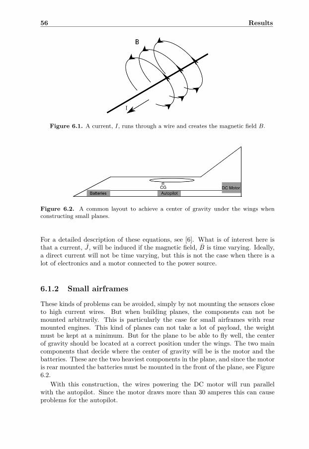
56 Results
Figure 6.1. A current, I, runs through a wire and creates the magnetic field B.
Figure 6.2. A common layout to achieve a center of gravity under the wings whenconstructing small planes.
For a detailed description of these equations, see [6]. What is of interest here isthat a current, J , will be induced if the magnetic field, B is time varying. Ideally,a direct current will not be time varying, but this is not the case when there is alot of electronics and a motor connected to the power source.
6.1.2 Small airframes
These kinds of problems can be avoided, simply by not mounting the sensors closeto high current wires. But when building planes, the components can not bemounted arbitrarily. This is particularly the case for small airframes with rearmounted engines. This kind of planes can not take a lot of payload, the weightmust be kept at a minimum. But for the plane to be able to fly well, the centerof gravity should be located at a correct position under the wings. The two maincomponents that decide where the center of gravity will be is the motor and thebatteries. These are the two heaviest components in the plane, and since the motoris rear mounted the batteries must be mounted in the front of the plane, see Figure6.2.
With this construction, the wires powering the DC motor will run parallelwith the autopilot. Since the motor draws more than 30 amperes this can causeproblems for the autopilot.

6.1 Perturbed magnetic fields 57
0 1 2 3 4 5 6 7 8−1
0
1Magnetometer
0 1 2 3 4 5 6 7 8−1
0
1
Nor
mal
ized
mag
netic
mea
sure
men
t
0 1 2 3 4 5 6 7 8−1
0
1
Time [s]
Figure 6.3. Normalized magnetometer measurements when aircraft is at stand-still withnormal wiring. After two seconds the engine is started.
6.1.3 Disturbance analysis
The effect of disturbances caused by the induced fields by the wires is analyzedby fixating the plane to the ground. The autopilot is mounted parallel to thewires powering the DC motor. In Figure 6.3 it is obvious that the magnetic fieldbecomes severely distorted when the motor starts after 2 seconds. The distortionwill be proportional to the current feeding the DC motor, so this is not a constantfield that can be compensated for in a simple way.
When the motor starts the magnetometer’s z-axis changes from a huge positivenumber to a huge negative number. In Sweden, the downward component of theearth’s magnetic field is the largest one. If it switches sign the magnetometer willindicate that the autopilot is upside down, so it is clear that these readings areuseless whilst the motor is running. As discussed, the magnetic field created by theelectrical current affected the magnetometer reading a lot, we can also see that thenoise level increases. That induced currents affects other MEMS sensors as well,which can be seen in Figure 6.4. When the motor starts after 2 seconds the noiselevel increases dramatically on the accelerometer, and this goes for all the sensors.The difference between the accelerometer and the magnetometer is that a bias isnot introduced, just an increase of noise. This can be understood from (6.1). Theinduced currents is caused by fluctuations in the magnetic field. Since the currentis not held constant in wires delivering power to the DC motor the magnetic fieldwill not be constant either. When the magnetic field temporarily increases it

58 Results
0 1 2 3 4 5 6 7 8−0.2
0
0.2Accelerometer
0 1 2 3 4 5 6 7 8−0.2
0
0.2
[m/s
2 ]
0 1 2 3 4 5 6 7 8−0.2
0
0.2
Time [s]
Figure 6.4. Accelerometer measurements when aircraft is at stand-still with normalwiring. After two seconds the engine is started.
will introduce currents in one direction, when the magnetic field decreases it willintroduce currents in the opposite direction. The output of the MEMS sensors areanalog and converted to digital values by an A/D converter. These fluctuationsin induced currents will cause temporary misreads by the A/D converter, andthis is the cause of the increased noise of the MEMS sensors. In Figure 6.5 thepart of the accelerometer measurement where the motor is running is cut out andplotted in the frequency domain. This gives information about the fluctuation inthe magnetic field caused by the wires in the fuselage. If a relationship betweenthe speed of the motor and the induced fluctuations can be described the noiseproblems can probably be solved by a notch filter. But even if this is successful,the problem with the magnetometer will still exist.
6.1.4 Minimizing electrical disturbancesIf possible, the cables powering the motor should not be placed parallel with theautopilot, if the construction of the aircraft allows this. With small aircraft thismight not be an option. The most obvious way to solve the problem is to useshielded cables.
A very simple way of reducing the noise is to twist the wire that delivers currentto the motor with the wire that connects back to the ground and to shield thecable with a metal foil or with a metal braiding and connect it to ground. Thiswill divert the magnetic field to a path through the foil or braiding so that the

6.2 GPS issues 59
0 10 20 30 40 50 60 700
0.5
1x 10
−4
Frequency [Hz]
Disturbed accelerometer frequenciesΦ
Figure 6.5. Frequency analysis of the electrically disturbed accelerometer.
disturbing magnetic field does not affect the autopilot. In an aircraft there is notrue ground, and therefore the battery’s ground should be used.
The cable constructed for these experiments consists of a braided and twistedcable. The metal braiding is connected to the ground. The same experimentas described in 6.1.3 is performed. How well the disturbing magnetic fields aresuppressed can be seen in Figure 6.6. The motor starts after 2 seconds, but thereis no indications of external magnetic fields. The accelerometer measurements canbe seen in Figure 6.7, and there is no longer an increase in noise levels when themotor starts.
From Section 6.1.3 we can see how important it is to minimize the electricaldisturbances that can be caused by improper wiring. A very simple, but veryeffective, way of improving the measurements that requires no special cables areproposed and should always be done if no shielded power cables to the motor areavailable.
6.2 GPS issuesWhen introducing movement to the system, the accelerometer could not be fusedwith the GPS. During the thesis, it became clear that an arbitrary GPS cannotbe used. In this section, experienced problems with the GPS are explained and asolution is proposed.
6.2.1 GPS ModesA GNSS is desirable to have in many different types of systems, from hand-helddevices to high speed aircraft. These two examples have very different requirementson the GNSS. For example, the pedestrian is not interested in momentary changesin position in velocity but wants to have a smooth position estimate with low noise.The aircraft on the other hand moves very fast and needs to know the momentaryposition. The manufacturers of GNSS chips often provides some kind of filteringin their modules. A typical hand-held device may have one second delay position

60 Results
0 2 4 6 8 10−1
0
1Magnetometer
0 2 4 6 8 10−1
0
1
Nor
mal
ized
mag
netic
mea
sure
men
t
0 2 4 6 8 10−1
0
1
Time [s]
Figure 6.6. Normalized magnetometer measurements when aircraft is at stand-still withshielded wiring. After two seconds the motor is started.
0 2 4 6 8 10−0.2
0
0.2Accelerometer
0 2 4 6 8 10−0.2
0
0.2
[m/s
2 ]
0 2 4 6 8 10−0.2
0
0.2
Time [s]
Figure 6.7. Accelerometer measurements when aircraft is at stand-still with shieldedwiring. After two seconds the motor is started.

6.2 GPS issues 61
0 2 4 6 8 10 1250
60
70
80
Time [s]
Hei
ght [
m]
GPSPitot
0 2 4 6 8 10 1260
80
100
120
Time [s]
Hei
ght [
m]
Comparison of GPS chip latency
GPSPitot
Figure 6.8. Two GPS chips measuring height compared to height derived from staticpressure measured by a pitot tube. The lower is a GPS set in pedestrian mode.
and velocity measurements due to extensive filtering. In this case this is desiredbecause the pedestrian moves slowly in small areas, and one second delay in themeasurements does not matter. On an aircraft moving in over 100m/s this can bedevastating, especially in real time systems, since it will always acquire a positionestimate that is 100m off. If internal filtering is turned off, noise on the positionand speed estimate will increase but the measurement will be up to date. In Figure6.8 two different GPS chips are used. The height from the GPS chips is comparedto the height indicated by a static pressure sensor.
Unfortunately, the latency is not always provided by the manufacturer, nor isit guaranteed.
6.2.2 Variable latencyEven though the mode of the GPS is important, this is something that can beevaluated by studying data sheets and second hand information. A problem thatwas discovered with the GPS used on the EasyPilot was variable latency. Thiswas hard to prove from collected data since the main accelerations in an airframeis during coordinated turns. It is difficult to generate plots that makes sense froma rotating accelerometer and a variable latency GPS.
The manufacturer of the chip provided information and plots that concludedthat there was variable latency on the GPS. These can however not be publisheddue to confidentiality.

62 Results
6.2.3 GPS conclusionsThe choice of GPS is not trivial, especially when GPS data is to be fused with othersensors. The GPS used on EasyPilot was considered not fit for high accelerationturning vehicles. With this said, it is probably not a bad GPS, it is only appliedto the wrong application.
For sensor fusion, low latency and little filtering is desired. If a GPS moduleis using extensive filtering, it will probably suffer in latency and the noise on theoutput is unknown.
The solution to the GPS problems is to replace it. A new GPS suitable for highacceleration applications should be used for EasyPilot to improve the abilities tofuse sensor data in a proper manner.
6.3 22 state EKFIn this section, the results of the 22 state EKF are presented.
6.3.1 Position and Velocity estimationThe position and velocity estimation did not work when adding GPS to the mea-surement equations of the EKF. It is difficult to know for sure why this is the case.When the GPS is added, the accelerometer bias states is estimated incorrectly andthe acceleration states will start to fluctuate. This has a great impact on gyro-scope bias and estimated orientation. From this point it is hard to interpret whatactually went wrong since all states seems to be estimated incorrectly.
There are four probable causes to this problem, or a combination of the three:
GPS latency: As described in Section 6.2, there was a very significant latencyfrom the GPS used on the autopilot. This means that the accelerometer andGPS will feed the filter with contradictory information during accelerationand deceleration.
GPS filtering: The GPS also had a very strange filter providing position esti-mates. It could be smooth for a while and then jump to another value.The inconsistency on the GPS estimates could cause strange behavior in thefilter.
Magnetic field disturbances: If there are magnetic field disturbances, the mag-netometer and accelerometer will feed the filter with contradictory informa-tion, thus causing the acceleration bias to be estimated incorrectly.
Improper tuning: The filter might be tuned incorrectly. It is a difficult task totune an EKF, especially when the cause of the problems are unknown.
During this master thesis, the conclusion that a combination of GPS latencyand internal GPS filtering is the probable cause has been taken. This is becauseit has been shown that the GPS has significant errors and because the filter isworking properly as long as there are no motions present.

6.3 22 state EKF 63
0 20 40 60 80 100 120−100
0
100
200Y
aw
Attitude
0 20 40 60 80 100 120−50
0
50
Pitc
h
0 20 40 60 80 100 120−50
0
50
Time [s]
Rol
l
EKF attitudeCurrent attitude
Figure 6.9. Estimated attitude by the EKF compared with the current attitude esti-mation on the autopilot.
6.3.2 Attitude estimation
Since no external references of the attitude are present, the tests are done in acontrolled environment. First, the autopilot is laying flat and still so that referencesfor gyro biases can be calculated. Then the following motions are performed:
Roll - Roll to 45, then roll back to original position.
Pitch - Pitch to 45, then pitch back to original position.
Yaw - Yaw 120 from original position, then yaw back to original position.
In Figure 6.9 the estimated attitude is presented. There is a good result in pitchand roll, but the yaw angle is converging slowly after the gyroscopes has updatedthe states. This is because there is very little information about the yaw angle fromthe available measurements. The earth’s magnetic field has very high inclinationin Sweden and the gravity is always pointing to the center of the earth. Because ofthis there is very little information in yaw angle. After the gyroscopes has updatedthe quaternions the yaw angle reaches approximately 110, then it takes almost20 seconds for the quaternions to converge.
This calls for careful calibration of the gyroscopes scaling factors. If the gy-roscopes are well calibrated, the other sensors would only need to stabilize theestimates whilst the gyroscopes takes care of the quaternion propagation.

64 Results
0 20 40 60 80 100 120−0.2
−0.1
0
Rol
l bia
s [r
ad/s
]
0 20 40 60 80 100 120−0.2
−0.1
0
Pitc
h bi
as [r
ad/s
]
0 20 40 60 80 100 120−0.06
−0.04
−0.02
0
Yaw
bia
s [r
ad/s
]
Time [s]
Estimated biasCalculated bias
Figure 6.10. Gyroscope biases estimated by the EKF compared with biases calculatedfrom mean.
6.3.3 Bias estimation
In Figure 6.10 the gyroscope biases are presented. These are of great importanceif the gyroscopes are to be used for propagation of the quaternions. The red lineis the calculated mean of the gyroscope measurements when the autopilot is atstand-still. The same discussion as for the attitude angles holds for this resultsto, there is little information from other sensors of the yaw-motion when orientedhorizontal. The bias in roll and pitch angle works fine since the magnetometerand accelerometer measurements does not change.
The accelerometer bias is harder estimate and also to evaluate. The truebias of the accelerometer is unknown, since the accelerometer output is based onorientation. To calculate true biases the exact position of the accelerometer chipmust be known. Unfortunately the accelerometer chip orientation is not known,so the error caused by orientation uncertainties would probably be larger than thebias.
The bias estimated by the filter can be seen in Figure 6.11. Here we cansee that the bias seems to converge to different values depending on orientation.One sensor that is used to estimate the bias in the Extended Kalman filter is themagnetometer. If the magnetometer and accelerometer is misaligned they willdeliver contradictory information about orientation. This conflict is resolved bythe Extended Kalman filter by changing the accelerometer biases. The conclusionfrom Figure 6.11 is that a sensor misalignment calibration might be necessary.

6.4 EKF wind estimation 65
0 20 40 60 80 100 120−0.5
0
0.5A
cc x
bia
s [m
/s2 ]
0 20 40 60 80 100 120−0.5
0
0.5
1
Acc
y b
ias
[m/s
2 ]
0 20 40 60 80 100 120−1
−0.5
0
Acc
z b
ias
[m/s
2 ]
Time [s]
Estimated bias
Figure 6.11. Accelerometer biases estimated by the EKF.
6.4 EKF wind estimationThe Extended Kalman Filter for wind estimation is based on the models derivedin 4.3. The test was performed with the autopilot flying the aircraft in a squareat fixed altitude. In Figure 6.12 we can see the GPS speed and the airspeedmeasured during the flight. The autopilot always flies by airspeed, and in thisflight the airspeed reference was set to 20 [m/s]. The weather information fromthe day of the flight indicated a wind at 5 [m/s].
From Figure 6.12 we can estimate the wind speed and direction by studying therelationship between airspeed and ground speed. When the ground speed is higherthan the indicated airspeed we are flying with tailwind and when the ground speedis lower we have a headwind. By measuring the distance between the valleys andthe peaks in the ground speed we can get a rough estimate of the speed of thewind according to
vw =vmaxg − vmin
g
2 . (6.3)
From the plots in Figure 6.12 we can get an indication that the wind speed issomewhere between 5 and 7 [m/s]. We can also look at interval where the groundspeed has it’s minimum and compare this with the heading. From the plots wecan see that the aircraft has it’s strongest headwind whilst heading 290 − 300.This indicates that we have a north-northwest wind at 5− 7 [m/s].
In Figure 6.13 the result of the Extended Kalman filter is illustrated. The windspeed is estimated to around −6 [m/s] and the heading of the wind is estimated to

66 Results
0 50 100 150 200 250 3000
20
40v a [m
/s]
0 50 100 150 200 250 3000
20
40
v g [m/s
]
0 50 100 150 200 250 3000
200
400
φ g [deg
]
Time [s]
Figure 6.12. Measured wind speed, ground speed from GPS and heading from GPS
around −65. Since north is defined as 0 we can add 360 degrees to our estimate,which gives an estimate of 295. When deriving the wind model we represent thewind as an angle and a speed, see Figure 4.1. This means that a negative windspeed at 295 is a positive wind speed in nort-northwest and this is what we wouldexpect from the flight pattern given in Figure 6.12.
The estimated state, Ka, was defined as a function of the slip angle and angle ofattack. Since this parameter fluctuates a lot the plane must have been flying withside slip or with an angle of attack. This induces uncertainties in the reasoningabout wind speed and wind direction from Figure 6.12 since we can not be surein which direction the plane is actually heading.
6.5 RLS parameter estimationThe RLS parameter estimation is used to estimate the constant, K, from (4.11).The estimation of this parameter is of importance if the GPS and static pressuresensor are to present the same altitude. In Figure 6.14 the GPS height, altitude

6.5 RLS parameter estimation 67
0 50 100 150 200 250 300−10
−5
0
v w [m
/s]
0 50 100 150 200 250 300−200
0
200
φ w [d
eg]
0 50 100 150 200 250 3000
2
4
Ka [m
/s]
Time [s]
Figure 6.13. Estimated parameters for the wind model. vw is the wind speed and φw
the wind direction.

68 Results
0 100 200 300 400 500 60040
60
80
100
120
140
160
180
Time [s]
Hei
ght [
m]
GPS heightStatic pressure without RLSStatic pressure with RLS
Figure 6.14. GPS height compared to height calculated from static pressure.
from the pressure sensor when K is constant and height from pressure sensor whenK is estimated with RLS in flight. As seen in the Figure, the GPS height variesa lot. In this measurement series, the curvature from the pressure sensor is seenas the more reliable of the two. Even though the form of the curvature is correct,it is clear that a constant offset is persistent when flying at cruising altitude. TheGPS does not have this weakness, even if the measurements fluctuates, it will nothave an offset. It is this characteristic from the GPS height that can be utilizedto improve the pressure measurement together with a RLS.
The updates should however be performed with care. After approximately 250seconds in flight, the GPS measurement becomes erroneous, dropping almost 60meters in a few seconds. If we follow the RLS adjusted height measurement, wecan see that after this moment the mean value becomes lower than the GPS height.This error has apparently affected the parameter estimation a lot and it takes timefor the parameter to converge to a correct value again. To avoid this problem, theRLS should not be invoked when the GPS height is considered unreliable.

Chapter 7
Conclusions and future work
7.1 ConclusionsIn this master thesis the goal was to design and evaluate an Extended KalmanFilter for state estimation of an UAV. Complementary filters for wind estimationand for height measurement improvements have been presented as well. The filtershave been implemented in Matlab, C# and C.
A large focus was put into the analysis of the magnetometer since it was con-sidered to be of importance in the Extended Kalman filter. It is a very goodsensor to have if it is working, but if it is not it will cause problems in the stateestimation. Unfortunately, it is also very sensitive to disturbances which means itmay become unreliable in an improper environment.
During the master thesis all work has been done using an existing autopilot withthe sensors mounted. This have caused restriction of the work in some aspects,no sensors could be exchanged and they had to be sampled through the existingAHRS. This meant that software for logging and an extension of the autopilotscommunication protocol had to be developed. With this configuration, the highestdelivery rate of sensor data was limited to 122Hz.
At a late stage of the master thesis data logging was done from actual flights.Around the mounting position of the autopilot there was major electrical andmagnetic disturbances. These problems have also been discussed and solved inthis master thesis.
Another issue that affects the possibilities to design this kind of ExtendedKalman filter is the GPS. When developing a filter of this type, an arbitraryGPS chip will not do. A GPS chip may have all kinds of internal filtering andlatencies. The GPS chip mounted on the used autopilot has increased latencywhen accelerating or decelerating, which means that the GPS and accelerometerwill feed the filter with contradictory information during short periods of time.Another GPS that have been used had a constant latency at over 1s, thus yieldingit useless.
During the beginning of the master thesis, when the sensors was evaluated andcalibration algorithms were derived, a calibration for sensor misalignment should
69
70 Conclusions and future work
have been derived as well. It is hard to confirm that there is a small misalignmenton the mounted sensors, but indications that this might be the case exists.
The attitude estimation of the Extended Kalman filter is not superior to thecurrent filter implemented in the AHRS. But the Extended Kalman Filter alsoestimates other states that is of interest in a controlled manner and eliminates theneed for manual calibration of biases. Although the Extended Kalman filter thathas been designed during this master thesis has a lot of benefits, in the state inwhich it is right now, it cannot compete with the robustness of the current AHRS.The steps required to make the Extended Kalman filter more robust consists offilter tuning, misalignment calibration, better GPS firmware and measurementsshould be audited if they are suitable for updating the filter.
7.2 Future workToday, micro controllers are becoming increasingly faster together with float pre-cision. This creates opportunities for implementing advanced filtering in real timesystem. Extended Kalman filters with complex state space models can now beupdated by many measurement equations in a satisfying frequency. The proposedExtended Kalman filter holds great potential for small UAVs since it is shownthat it is possible to use the filter with commercially available MEMS sensors andpower efficient MCU’s. Future work should be focused on the robustness of theExtended Kalman filter.
Another very interesting competitor to the Extended Kalman filter is the Un-scented Kalman filter. This is a filter that handles the non-linearity problem in abetter way than the Extended Kalman filter. Instead of calculating the Jacobians,the Unscented Kalman filter utilizes the Unscented transform to calculate sigmapoints. These are then propagated through the non-linearities. Since there arenon-linearities in the quaternions the UKF may perform better than the EKF inthis case.

Bibliography
[1] Cenk Acar and Andrei Shkel. MEMS Vibratory Gyroscopes: Structural Ap-proaches to Improve Robustness.
[2] David W. Allan. Statistics of atomic frequency standards. Proceedings of theIeee, 54(2), 1966.
[3] Cho Am, Kim Jihoon, Lee Sanhyo, and Changdon Kee. Wind estimationand airspeed calibration using the uav with a single-antenna gnss receiverand airspeed sensor. Technical report, School of Mechanical and AerospaceEngineering, Seoul National University, Korea, 2006.
[4] Frank J. Centinello III. Analysis of the ned and ecef covariance propaga-tion for the navigational extended kalman filter. International AstronautigalCongress, 58, 2007.
[5] Tom Chalko. High accuracy speed measurement using gps (global positioningsystem). Nujournal, 2007.
[6] K David Cheng. Field and Wave Electromagnetics.
[7] Mark Euston, Paul Coote, Robert Mahoney, Jonghyuk Kim, and TarekHamel. A complementary filter for attitude estimation of a fixed-wing uav.Technical report, Automation and Robotics Laboratory - Aveiro University.
[8] Fredrik Gustafsson. Statistical Sensor Fusion. 1 edition, 2010. ISBN13: 978-91-44-05489-6.
[9] Fredrik Gustafsson, Lennart Ljung, and Mille Millnert. Signal Processing. 1edition, 2010. ISBN13: 978-91-44-05835-1.
[10] Willem J. Hough. Autonomous aerobatic flight of a fixed wing unmannedaerial vehicle. Master’s thesis, Stellenbosch University, 3 2007.
[11] I.Markovsky, A.Kukush, and S.Van Huffel. Consistent least squares fitting ofellipsoids. Numerische Mathematik, 98:177–194, 2004.
[12] Fredrik Johansson and Hugo Kinner. Sensorfusion för reglering av obemannadhelikopter. Master’s thesis, Linköping University, 2011.
71

72 Bibliography
[13] Rudolf E. Kalman. A new approach to linear filtering and prediction problems.Journal of Basic Engineering, 82(Series D), 1960.
[14] J L Marins, E R Bachmann, R B McGhee, and M J Zyda. An extendedkalman filter for quaternion-based orientation estimation using marg sensors.Proceedings 2001 IEEERSJ International Conference on Intelligent Robotsand Systems Expanding the Societal Role of Robotics in the the Next Mil-lennium Cat No01CH37180, 4(2):2003–2011, 2003.
[15] Joao L. Marins. An extended kalman filter for quaternion-based attitudeestimation. Master’s thesis, United States Navy - Naval Postgraduate School,9 2000.
[16] Valérie Renaudin, Muhammad Haris Afzal, and Gérard Lachapelle. Completetriaxis magnetometer calibration in the magnetic domain. Journal of sensors,2010, 10 2010. ID 967245.
[17] Sven Rönnback. Development of a ins/gps navigation loop for an uav. Mas-ter’s thesis, LuleåTekniska Universitet, 2 2000.
[18] Inc. SiRF Technology. NMEA Reference Manual. SiRF Technology, Inc., 2.1edition, February 2007. Part Number: 1050-0042.
[19] Sensors Spectrum and Controls Inc. Compensating for accelerometer mis-alignments. Tech Note 413.
[20] Sherryl H. Stovall. Basic inertial navigation. Technical report, Nav-igation and Data Link Sectionm, Systems Integration Branch, 1997.http://www.fas.org/spp/military/program/nav/basicnav.pdf.
[21] David Titterton and John Weston. Strapdown Inertial Navigation Technol-ogy. The Institution of Electrical Engineers, 2 edition, 2004.
[22] David Törnqvist. Estimation and Detection with Applications to Navigation.PhD thesis.
[23] David Törnqvist. Statistical fault detection with applications to imu distur-bances.
[24] u-blox ag, http://www.u-blox.ch. Datum Transformation of GPS Position, 71999.
[25] Martin Vagner. Mems gyroscope performance comparison using allan variancemethod. Technical report, FEEC BUT.
[26] Clas Veiback. Automatic control of unmanned aerial vehicles. Master’s thesis,Uppsala University, 2010.
[27] Jean-Marie Zogg. Gps, essentials of satellite navigation. Technical ReportGPS-X-02007-D, U-blox AG, 2009.

Appendix A
Linearization
When linearizing model and measurement equation the partial derivative is takenwith respect to all states. The state space used to describe the linearizations hereare Model 2 as depicted in Section 4.2 with 24 states,
x =
pvaqωbabωw
(A.1)
The point of linearization will be denoter x0 throughout this appendix. Only thenon zero parts of the linearization are presented.
Model linearizationThe non linear parts of the model consists of p = P (p)v and q = S(ω)q. Allother states in the presented models are linear.
Position propagation
The position propagation is given by
p = P(p) · v. (A.2)
In matrix form this is λφh
=
0 1(a+h) cosφ 0
1a+h 0 00 0 h
. (A.3)
73

74 Linearization
The partial derivative with respect to p and v is then given byλφh
= (A.4)
0 VE sinφ((a+h) cosφ)2
−VE cosφ((a+h) cosφ)2 0 1
(a+h) cosφ 00 0 −VN
(a+h)21
a+h 0 00 0 0 0 0 −1
∣∣∣∣∣∣∣x=x0
λφhVNVEVD
(A.5)
=[Hp Hv 03×18
]x (A.6)
Quaternion propagation
The quaternion propagation is given by equation (2.50),
q = 12S(ω)q = 1
2 S(q)ω. (A.7)
The linearization parts are given by
Hq = ∂(0.5S(ω)q∂q ) = 0.5S(ω) (A.8)
Hw = ∂(0.5S(q)ω∂ω
) = 0.5S(q). (A.9)
This gives the linearized states as
q =[04×9 S(ω) S(q) 04×8
]x (A.10)
Measurement linearizationThere are three non linear measurement equation presented in Section 4.2.1, ac-celerometer, magnetometer and pitot tubes. The linear equations are not presentedhere and are unchanged from Section 4.2.1 when implementing the filter.
Accelerometer
The measurement equation, as in equation (4.19), is given by
yacc = Cnb (q)(a − g)− bacc + eacc. (A.11)
The rotation matrix Cnb (q) and acceleration a − g is given by
Cnb (q) =
q20 + q2
1 − q22 − q2
3 2(q1q2 + q0q3) 2(q1q3 − q0q2)2(q1q2 − q0q3) q2
0 − q21 + q2
2 − q23 2(q2q3 + q0q1
2(q1q3 + q0q2) 2(q2q3 − q0q1) q20 − q2
1 − q22 + q2
3
(A.12)
a =
aNaE
aD − g
(A.13)

75
Taking the derivative with respect to a, q and bacc respectively gives
Haa = ∂yacc
∂a
∣∣∣∣x=x0
= Cnb (q)|x=x0(A.14)
Haq = ∂yacc
∂q
∣∣∣∣x=x0
=
Haq,1
Haq,2
Haq,3
(A.15)
Hba = I3×3 (A.16)
where
Haq,1 =
q0q3−q2
T a
q1q2q3
T a
−q2q1−q0
T a
−q3q0q1
T a
(A.17)
Haq,2 =
−q3q0q1
T a
q2−q1q0
T a
q1q2q3
T a
−q0−q3q2
T a
(A.18)
Haq,3 =
q2−q1q0
T a
q3−q0−q1
T a
q0q3−q2
T a
q1q2q3
T a
. (A.19)
The linearized measurement equation then becomes
yacc =[03×6 Ha
a Haq 03×3 Hb
a 03×5]x (A.20)
Magnetometer
The measurement equation, as in equation (4.28), is given by
ymag = Cnb (q)Bearth + eacc (A.21)
The magnetic reference field generated by the earth is seen as a constant. Theonly non zero component in the measurement equation is then given by
Hmq = ∂ymag
∂q
∣∣∣∣x=x0
=
Hmq,1
Hmq,2
Hmq,3
(A.22)

76 Linearization
where
Hmq,1 =
q0q3−q2
T B
q1q2q3
T B
−q2q1−q0
T B
−q3q0q1
T B
(A.23)
Hmq,1 =
−q3q0q1
T B
q2−q1q0
T B
q1q2q3
T B
−q0−q3q2
T B
(A.24)
Hmq,3 =
q2−q1q0
T B
q3−q0−q1
T B
q0q3−q2
T B
q1q2q3
T B
. (A.25)
The linearized magnetometer measurement then becomes
ymag =[03×9 Hm
q 03×11]x (A.26)