Charles University in Prague

Faculty of Social Sciences

Institute of Economic Studies

Master Thesis

2012 Jakub Stračina

CHARLES UNIVERSITY IN PRAGUE

FACULTY OF SOCIAL SCIENCES

Institute of Economic Studies

Austrian Business Cycle Theory and the

Recession of 2007-2009 in the US Economy

Master Thesis

Author: Bc. Jakub Stračina

Supervisor: Mgr. Pavel Ryska, MPhil

Academic Year: 2011/2012

I wish to express my gratitude towards Pavel Ryska for his positive approach

and helpful insights. I also wish to thank my parents for their unquestionable

support and understanding of my choices.

Declaration

I hereby declare that I created this master thesis independently, using only the

listed literature and resources.

Prehlásenie

Prehlasujem, že som diplomovú prácu vypracoval samostatne a použil výhradne

uvedené zdroje a literatúru.

Prague, January 9, 2012 .....................................................

Abstract

This paper aims to evaluate merits of the Austrian business cycle theory in explaining the

2001-2009 business cycle in the US economy. The theory postulates that a monetary shock

upsets equilibrium in the market for loanable funds and adversely influences coordination

mechanisms of the economy. The structure of relative prices is distorted and resources are

misallocated as a result. The economy follows an unsustainable investment trajectory

inconsistent with the amount of available resources and with the consumer preferences. When

the inconsistencies are revealed, some of the investments are liquidated and costly correction

follows. After providing exposition of the theory and description of the US economy in 2001-

2009, the theory is confronted with the data. Although some deviations are conceded, mainly

in development of the labor market, analysis presented in the paper supports the Austrian

business cycle theory as a solid theoretical tool for explanation of the economic development

throughout the examined period. The theory exhibits its main strengths in accounting for

development of relative prices and linking them to conditions in the market for loanable

funds.

Abstrakt

Cieľom tejto práce je zhodnotiť význam rakúskej teórie hospodárskeho cyklu pri vysvetlenie

hospodárskeho cyklu rokov 2001-2009 v ekonomike USA. Teória postuluje schopnosť

monetárneho šoku narušiť alokačné mechanizmy v ekonomike. V dôsledku toho dochádza

k deformácii štruktúry relatívnych cien a tomu zodpovedajúcej misalokácii zdrojov.

Ekonómia tak nasleduje neudržateľnú investičnú trajektóriu, ktorá je nekonzistentná

s dostupnosťou zdrojov a preferenciami spotrebiteľov. Pri odhalení nekonzistencii sú niektoré

investície likvidované a nasleduje nákladná korekcia. Práca podáva výklad teórie, stručný

popis ekonomiky USA v období 2001-2009 a konfrontáciu teórie s datami. Napriek

pripusteniu niektorých odchýlok, hlavne vo vývoji pracovného trhu, analýza prezentovaná

v práci podporuje rakúsku teóriu hospodárskeho cyklu ako silný teoretický nástroj

k vysvetleniu ekonomických udalostí skúmaného obdobia. Ako hlavnú silu teórie možno

identifikovať jej schopnosť vysvetľovať vývoj relatívnych cien v súvislosti s podmienkami na

trhu zápožičných fondov.

CONTENTS

1. Introduction ........................................................................................................................1

2. The Theory .........................................................................................................................3

2.1 Origins ..........................................................................................................................3

2.2 Credit Expansion as a Monetary Shock .........................................................................5

2.3 Structure of Production and the Hayekian Triangle .......................................................5

2.4 Economic Growth and the Structure of Production ........................................................7

2.4.1 The Secular Growth ...............................................................................................7

2.4.2 Discount Effect ......................................................................................................9

2.4.3 Increase in Savings and a Sustainable Economic Expansion ................................. 10

2.4.4 Credit Expansion and the Cycle-generating Boom ................................................ 12

2.5 Expansion to Contraction ............................................................................................ 14

2.5.1 Malinvestment and Overconsumption .................................................................. 14

2.5.2 The Reversal ........................................................................................................ 15

2.6 Interest Rates .............................................................................................................. 17

2.6.1 Magnitude of Interest Rates .................................................................................. 18

2.6.2 Liquidity Effect .................................................................................................... 18

2.7 Relative Prices throughout the Business Cycle ............................................................ 19

2.7.1 Dynamics of the Structure of Prices ..................................................................... 20

2.8 Expectations and the ABCT ........................................................................................ 23

2.8.1 The Critique ......................................................................................................... 23

2.8.2 Prisoner’s Dilemma and Irrelevance of Knowledge .............................................. 24

2.8.3 Limits of Knowledge and the Possibility of Correct Expectations ......................... 26

3 Application: US Economy 2001- 2009 ............................................................................... 29

3.1 Propositions ................................................................................................................ 29

3.2 Macroeconomic Description of the Period .................................................................. 31

3.2.1 Gross Domestic Product ....................................................................................... 31

3.2.2 HOUSING MARKET .......................................................................................... 32

3.2.3 Unemployment ..................................................................................................... 34

3.2.4 Federal Reserve’s Policy and Monetary Development .......................................... 35

3.2.5 Consumer Price Inflation ...................................................................................... 41

3.2.6 Stock Market ........................................................................................................ 41

3.3 Credit Expansion and the Market for Loanable Funds ................................................. 42

3.3.1 Investment and Saving ......................................................................................... 43

3.3.2 Proposition 1: Credit Becomes Detached from Savings ........................................ 44

3.3.3 Proposition 2: The Liquidity Effect ...................................................................... 45

3.4 Sectoral Patterns and the Labor Market ....................................................................... 47

3.4.1 Proposition 3: Industrial Activity and the Structure of Production ........................ 50

3.4.2 Proposition 4: Wage Growth ................................................................................ 52

3.4.3 Proposition 5: Job Loss Pattern ............................................................................ 55

3.5. Relative Prices ........................................................................................................... 57

3.5.1 Commodity boom of 2006-2008 ........................................................................... 57

3.5.2 Proposition 6: Consumer and Producer Prices during the Credit Expansion .......... 61

3.5.3. Proposition 7: Prices Along the Structure of Production ...................................... 62

3.5.4 Relative Prices and the Stock Market ................................................................... 66

3.5.5 Proposition 8: Correction of the Distorted Relative Prices .................................... 67

4. Conclusion ....................................................................................................................... 75

References ............................................................................................................................ 77

Appendix .............................................................................................................................. 80

List of Figures

Figure 1: The Hayekian Triangle ............................................................................................6

Figure 2: The Market for Loanable Funds ...............................................................................8

Figure 3: Production Possibility Frontier ................................................................................8

Figure 4: Secular Growth ........................................................................................................9

Figure 5: Discount Effect Example ....................................................................................... 10

Figure 6: Fall in Time Preferences ........................................................................................ 11

Figure 7: Voluntary Increase of Savings ............................................................................... 12

Figure 8: Overconsumption and Malinvestments in the Hayekian Triangle ........................... 13

Figure 9: The Boom and Bust Cycle Trajectory and the PPF................................................. 15

Figure 10: Credit Expansion-induced Boom and Subsequent Bust ........................................ 16

Figure 11: Discounted Marginal Product along the Structure of Production .......................... 21

Figure 12: US Real GDP Annual Growth ............................................................................. 31

Figure 13: Homeowners' Equity and Industrial Activity ........................................................ 33

Figure 14: Unemployment .................................................................................................... 34

Figure 15: Target Policy Rate ............................................................................................... 36

Figure 16: Monetary Aggregates........................................................................................... 37

Figure 17:Federal Reserve Balance Sheet Development........................................................ 38

Figure 18: Fed's Reserve Requirements Policy ($Million) ..................................................... 39

Figure 19: Cumulative Cuts in Total Reserve Requirements ................................................. 40

Figure 20: Reserves and Money Base ................................................................................... 40

Figure 21: CPI Inflation ........................................................................................................ 41

Figure 22: Stock Market ....................................................................................................... 42

Figure 23: Savings and Investment ....................................................................................... 43

Figure 24: Credit Expansion and the Savings Gap ................................................................ 43

Figure 25: Causality between Credit and Savings ................................................................. 44

Figure 26: Yield Curve Slope ............................................................................................... 46

Figure 27: Yield Curve May 2004 ........................................................................................ 46

Figure 28: Yield Curve March 2007 ..................................................................................... 47

Figure 29: Expected Structure of Production ......................................................................... 49

Figure 30: Employment by Sectors ....................................................................................... 51

Figure 31: Industry-specific Impact of Credit........................................................................ 52

Figure 32: Cumulative Wage Growth ................................................................................... 54

Figure 33: Total Wage Growth in the Expansion Period ....................................................... 54

Figure 34: Credit Expansion and Unemployment .................................................................. 55

Figure 35: Cumulative Job Losses by Sectors ....................................................................... 56

Figure 36: Timing of Job Losses by Industry ........................................................................ 56

Figure 37: Total Job Losses by Industry ............................................................................... 56

Figure 38: Commodity Classes ............................................................................................. 58

Figure 39: S&P Goldman Sachs Commodity Index .............................................................. 59

Figure 40: Credit Expansion and Commodity Prices ............................................................. 60

Figure 41: Credit and PPI/CPI Ratio ..................................................................................... 61

Figure 42: Prices at Different Stages of Production (All) ...................................................... 63

Figure 43: Prices at Different Stages of Production (Energy Industry) .................................. 64

Figure 44: Prices at Different Stages of Production (Food Industry)...................................... 65

Figure 45: Dow Jones and Sub-indices (2002=100) .............................................................. 66

Figure 46: Price Differentials 1 (All) .................................................................................... 68

Figure 47: Price Differentials 2 (All) .................................................................................... 69

Figure 48: Price Differentials 3 (All) .................................................................................... 69

Figure 49: Price Differentials 1 (Energy Industry) ................................................................ 70

Figure 50: Price Differentials 2 (Energy Industry) ................................................................ 71

Figure 51: Price Differentials 1 (Food Industry) .................................................................... 71

Figure 52: Price Differentials 2 (Food Industry) .................................................................... 72

Figure 53: Price Differentials 3 (Food Industry) .................................................................... 73

Figure 54: Price Differentials (Summary) ............................................................................. 74

1

1. INTRODUCTION

After the recovery from the recession of 2001, the United States economy saw a period of

robust growth. The growth was associated with decreasing unemployment and vigorous

growth of the stock market. Although asset prices, particularly real-estate, were rapidly

increasing, inflation of consumer prices was seen as reasonably low. After a period of

seemingly favorable and unproblematic development, a sharp recession arrived at the end of

2007. The recession had a strong impact on the household sector through sharp downturn in

the housing market. The financial sector suffered from a series of blows in the form of

defaults, bankruptcies, forced mergers, losses, lack of liquidity and general uncertainty.

The surprising onset of the recession motivated and nourished discussions about its causes.

Different views on the subject and their clashes have drawn more attention. Business cycle

theorizing has become more relevant as a topic in economics and received more attention

even from outside of the economic profession. The present paper is a contribution to the on-

going debate. Its key aim is to examine the business cycle of 2001-2009 and the recession of

2007-2009 in the US economy from perspective of the Austrian business cycle theory.

The theory in its modern version is largely attributed to the works of Ludwig von Mises and

Friedrich von Hayek. It postulates that a monetary shock in the form of credit expansion

unsupported by an adequate level of savings leads to disequilibrium in the market for loanable

funds. Such imbalance in turn distorts interest rates and the structure of relative prices in the

economy. As a result the price signals fail to convey correct information and resources are

misallocated. The economy is sent on an unsustainable growth path, with investment projects

uncoordinated with consumer preferences. Furthermore, due to distorted price signals,

investment decisions are inconsistent with the amount of resources available for completion

of the investment projects. When the inconsistencies are revealed, the corrective reallocation

of resources in the form of recession follows.

After providing a comprehensive exposition of the theory and a brief description of the US

economy during the 2001-2009, the paper will proceed to confront the theory with economic

data from the period. The application is structured into 3 key areas and 8 propositions implied

by the theory. The first area aims at verification of the underlying conditions required by the

theory in order for the business cycle-generating mechanism to be set into motion. The other

two areas focus on particular patterns of economic development in expansion and contraction

phase of the economy.

2

The examined period starts in November 2001, when the National Bureau of Economic

Research declared end of the previous recession and ends in December 2009, a half a year

after the official end of the recession of 2007-2009. The paper focuses on diagnostics of the

business cycle phenomenon. We aim to determine whether the Austrian business cycle theory

provides a valid explanation of the business cycle in question. The present paper doesn’t

elaborate on policy implications in regard to preventing the business cycle or fostering the

economic recovery.

3

2. THE THEORY

Aim of the following section is to provide a comprehensive exposition of the Austrian

business cycle theory (ABCT) and enable better understanding of its application on the US

economy. After a brief overview of its origins, we shall lay out causal mechanism of business

cycle generation as postulated by the theory. In description of the causal chain that leads to

the cycle, we will largely draw on Garrison (2001 and 2004). The main advantage of

Garrison’s exposition is the synthesis of the theory with terminology and diagrams used in

modern macroeconomics, thus largely allowing omission of the terminological discussion.

Other major sources for the exposition of the theory include works of Hayek (1931 and 1975)

and Mises (1963 and 1978). Before proceeding to empirical application on the US economy,

we shall provide overview of rational expectations debate related to the Austrian business

cycle theory at the end of the theoretical chapter, as it has been the single most important

point of criticism.

2.1 ORIGINS

The Austrian Business Cycle Theory (ABCT) can be traced back to several precursors such as

David Hume, Knut Wicksell, David Ricardo, Henry Thorton and the British currency school

in general. Their theorizing began with an observation of the multiplication process; a

banking sector’s capacity to expand credit and induce monetary inflation. Their theoretical

advances consisted in following the effects of the credit expansion on economic activity and

its sustainability.

Ricardo and Thorton were the first economists to develop a monetary based business cycle

theory with some resemblances of the modern ABCT (de Soto 1998). Ricardo focused on

external drain of gold reserves from a country in which there was a significant monetary

expansion, namely expansion of bank notes on the top of gold reserves. Such inflationary

expansion would then lead to outflow of notes to countries where such monetary inflation has

not taken place (or has taken place at lower rate). Notes would then be redeemed for gold,

causing the drain of gold from the inflating country. As the gold reserves decrease relative to

issued paper notes, the money supply becomes top-heavy and volatile, as there is insufficient

gold to satisfy all the redemption requests. In order to decrease the bankruptcy risks, banks

contract credit supply and economic activity reverses.

4

The currency school business cycle theorizing can be seen as an early attempt towards the

ABCT. According to Mises, the currency school “failed to recognize that deposits subject to

check are money-substitutes and, as far as their amount exceeds the reserve kept, fiduciary

media, and consequently no less a vehicle of credit expansion than are banknotes” (Mises

1963, p. 440). A present day version of such fallacy would be to only count printing paper

bank notes as inflating money supply, but to leave out increases in the volume of demand

deposits. Rothbard (1969) views failure to address development of relative prices throughout

the business cycle as a major shortcoming of the currency school.

Wicksell’s contribution consists in focusing on the interest rates. Wicksell devised the term

“natural rate of interest”, referring to the rate that equilibriates the market for loanable funds

or, in other words, savings and investment. He then viewed deviations of the actual interest

rate, which he referred to as “money rate of interest,” from the natural rate as a distorting

phenomenon. If money rate of interest is pushed below the natural rate, credit financed

investments become more profitable and an artificial boom occurs, as banks can grant loans

beyond their saving deposits under the modern fractional reserve banking system. He referred

to the investment pattern following money rate divergence from the natural rate as a

cumulative process. He also alludes at restructuring of the structure of production that occurs

in the boom phase, which is a distinct feature of the ABCT. He however doesn’t draw any

conclusions about business cycle causality from his observations:

“…a mass of circulating capital is transformed into fixed capital, a process which, as I have

said, accompanies every rising business cycle: it seems as a matter of fact to be the one really

characteristic sign, or one in any case which it is impossible to conceive as being absent.”

(Wicksell 1962, p. 9)

Significant theoretical advances, especially with regard to theory of capital, were made by

economists of the early Austrian school, Carl Menger (Principles of Economics, 1871) and

Eugen von Bohm-Bawerk (The Positive Theory of Capital, 1888). The ideas were later

incorporated into ABCT by Mises and Hayek.

The clear link of the relative prices, structure of production and interest rates to the business

cycle phenomenon was first asserted by Mises, particularly in his Theory of Money and Credit

(1921). Notable contributions, especially in the field of relating changes in the structure of

production to the business cycle, were added by Hayek. Monetary Theory and Trade cycle

(1929) and Prices and Production were Hayek’s key contributions to the business cycle

5

theory. Hayek’s Nobel prize of 1974 (jointly awarded to him and Gunnar Myrdal) was

partially a recognition of his business cycle theorizing, "for their pioneering work in the

theory of money and economic fluctuations and for their penetrating analysis of the

interdependence of economic, social and institutional phenomena." (Nobel Committee, 1974)

ABCT’s expositions by Hayek and Mises have become a cornerstone of its further

development. A notable more recent contribution is Garrison’s Time and Money:

Macroeconomics of Capital Structure (2001), as it attempts to present ABCT using

terminology and graphical interpretation of neoclassical economics.

2.2 CREDIT EXPANSION AS A MONETARY SHOCK

ABCT postulates that a monetary shock can trigger a temporary unsustainable expansion. The

economic expansion however results from distorted signals, is incompatible with underlying

fundamentals and will necessarily end in a recession. By a monetary shock, we mean a bank

credit expansion that is not supported by a corresponding supply of saving. If supply of credit

rises due to increase in saving, a monetary shock doesn’t take place. If credit expands as a

result of the money multiplication process under fractional reserve lending, we refer to the

situation as monetary shock, or a credit expansion unsupported by savings. Policy decisions

that can enable or foster such an expansion include changes in reserve requirements, central

bank’s target policy rate setting and shielding commercial banks from the risk associated with

the fractional reserve lending practices (the lender of last resort role). There has been a rich

debate over possibility of bank credit expansion and its extent without such policy

interventions.1 We shall refer to credit expansion unsupported by savings as a policy-induced

boom, as there are clearly identifiable measures that at the minimum add to the extent of the

expansion.

2.3 STRUCTURE OF PRODUCTION AND THE HAYEKIAN TRIANGLE

One of the distinct features of the Austrian approach is disaggregating capital. Viewing

capital as homogeneous stock conceals dynamics of economic growth or, as Hayek put it, the

mechanics of change. The first step towards understanding the structure of production is a

distinction between the consumer goods and the producer goods. Generally speaking,

consumer goods are those that are sold to be consumed and do not represent inputs to any

1 See for example Competition and Currency: Essays on Free Banking and Money by Lawrence White (1989)

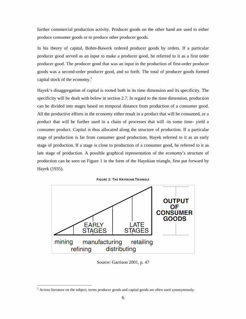
6

further commercial production activity. Producer goods on the other hand are used to either

produce consumer goods or to produce other producer goods.

In his theory of capital, Bohm-Bawerk ordered producer goods by orders. If a particular

producer good served as an input to make a producer good, he referred to it as a first order

producer good. The producer good that was an input in the production of first-order producer

goods was a second-order producer good, and so forth. The total of producer goods formed

capital stock of the economy.2

Hayek’s disaggregation of capital is rooted both in its time dimension and its specificity. The

specificity will be dealt with below in section 2.7. In regard to the time dimension, production

can be divided into stages based on temporal distance from production of a consumer good.

All the productive efforts in the economy either result in a product that will be consumed, or a

product that will be further used in a chain of processes that will -in some time- yield a

consumer product. Capital is thus allocated along the structure of production. If a particular

stage of production is far from consumer good production, Hayek referred to it as an early

stage of production. If a stage is close to production of a consumer good, he referred to it as

late stage of production. A possible graphical representation of the economy’s structure of

production can be seen on Figure 1 in the form of the Hayekian triangle, first put forward by

Hayek (1935).

FIGURE 1: THE HAYEKIAN TRIANGLE

Source: Garrison 2001, p. 47

2 Across literature on the subject, terms producer goods and capital goods are often used synonymously.

7

The height of the triangle represents value of the consumer goods produced in the economy.

Its length corresponds to the length of the longest production process (from resource

extraction to sale of consumer goods to the end consumer). It should be noted that not all

consumer goods are yielded by process with duration equal to the entire triangle’s length.

Production processes create a whole spectrum of durations. Some, such as turning a wild

forest berry into a consumer good by picking it up, require just very little time. Industry labels

under the triangle are examples of production activities along the structure of production.

Height of the triangle at any certain point of time can be seen as cumulative value of output at

that point of time. We shall use the Hayekian triangle as a graphic representation of the

economy’s structure of production, and refer to its stages as (relatively) early and (relatively)

late.

2.4 ECONOMIC GROWTH AND THE STRUCTURE OF PRODUCTION

In order to demonstrate causal chain that leads from a monetary shock to a business cycle, we

shall now examine three possible situations of growth in relation to the economy’s structure

of production.

2.4.1 THE SE C UL A R GR OWTH

The slope of the Hayekian triangle’s hypotenuse represents the distribution of available

investment funds along the time structure of production and reflects, as will be further

explained, the time preferences of lenders and borrowers in the economy. We will start with

unchanged time preferences of economic agents, then focus on their changes. First, as a

proportion of output, saving and consumption are constant.

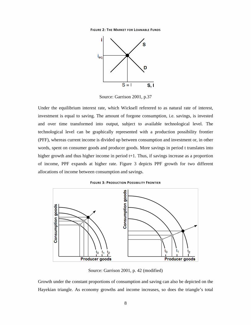
We start from equilibrium in the market for loanable funds (Figure 2). To simplify the

theoretical discussion, we shall abstract from the term structure of interest rates, risk

premiums and inflationary expectations. We shall treat interest rate as a product of time

preferences prevailing among the economic agents, revealed in their decisions to save and

consume certain proportions of present income.

8

FIGURE 2: THE MARKET FOR LOANABLE FUNDS

Source: Garrison 2001, p.37

Under the equilibrium interest rate, which Wicksell referered to as natural rate of interest,

investment is equal to saving. The amount of forgone consumption, i.e. savings, is invested

and over time transformed into output, subject to available technological level. The

technological level can be graphically represented with a production possibility frontier

(PFF), whereas current income is divided up between consumption and investment or, in other

words, spent on consumer goods and producer goods. More savings in period t translates into

higher growth and thus higher income in period t+1. Thus, if savings increase as a proportion

of income, PPF expands at higher rate. Figure 3 depicts PPF growth for two different

allocations of income between consumption and savings.

FIGURE 3: PRODUCTION POSSIBILITY FRONTIER

Source: Garrison 2001, p. 42 (modified)

Growth under the constant proportions of consumption and saving can also be depicted on the

Hayekian triangle. As economy growths and income increases, so does the triangle’s total

9

area. Constant allocation between consumption and saving is reflected in unchanged slope of

the triangle’s hypotenuse. Time preferences are unchanged, both savings and investment

increase at a constant rate and are equilibriated by the same level of interest rate (Figure 4).

FIGURE 4: SECULAR GROWTH

Source: Garrison (2001), p. 54

Garrison (2001) refers to such a steady growth as secular growth:

“Secular growth occurs without having been provoked by policy or by technological advance

or by a change in intertemporal preferences. Rather, the ongoing gross investment is

sufficient for both capital maintenance and capital accumulation.” (p. 54)

2.4.2 D I SC OU NT EF F E C T

Before proceeding with exposition of the theory, we need to establish that changes in interest

rate have an asymmetric impact across the structure of production. Let us demonstrate the

simple fact of long-term projects being more sensitive to discount rate changes on a numerical

example. Figure 5 displays a set of investment projects with a one-off identical initial

investment of 100. Every project has a different duration; from one to five periods. Every

project yields a one-off final pay-off at the end of its duration.

10

FIGURE 5: DISCOUNT EFFECT EXAMPLE

T0 T1 T2 T3 T4 T5 NPV

(d=10%)

NPV

(d=5%)

Project 1 -100 110 - - - - 0 4.54

Project 2 -100 0 121 - - - 0 9.29

Project 3 -100 0 0 133 - - 0 14.26

Project 4 -100 0 0 0 146 - 0 19.48

Project 5 -100 0 0 0 0 161 0 24.94

The final pay-off is set in order to make net present value (NPV) equal zero for the discount

rate of 10%. Thus, we have 5 projects with different durations, identical required initial

investments and identical NPV. Now suppose the discount rate is reduced to 5%. NPV of

every project is increased, however the longer the duration of a project, the greater the

increase.

Changes of NPV resulting from the changed discount rate can be directly related to what

Hayek referred to price margins between products at different stages of production. In the

state of equilibrium, there are no price margins. Resources are directed at investment projects

until the opportunities are equalized in terms of expected profitability. Assuming no

uncertainty, an entrepreneur with 100 to invest is indifferent between the 5 projects from the

example.3 With a change of discount rate, the investment funds will be relocated until the new

equilibrium is established and NPV of available investment projects equalized. In the case of

reduced discount rate, all investment projects become more profitable, but those with

lengthier production periods become relatively more profitable. We shall further elaborate on

this topic in the section on relative prices further below.

2.4.3 INC RE A SE I N SAV IN GS AN D A SUS TAI NA BL E EC O NOMIC EX PAN SI ON

Let us now assume the time preferences fall and the saving rate increases. More funds are

available for investment and less output is consumed, which leads to downward pressure on

investments into late stages of production (those in temporal proximity to consumption).

Preference for the present over future consumption is weakened. Consumption falls.

Relatively more investments are made into earlier stages of production. Moreover, new stages

3 For the sake of simplicity, we abstract from term premiums and assume no hyperbolic discounting

11

of production are realized and the production process lengthens. The change is depicted in

Figure 6.

FIGURE 6: FALL IN TIME PREFERENCES

(1) denotes the decrease in consumption and (2) the increase in investments. Lengthening of

the triangle corresponds to new stages of production. Slope of the triangle’s hypotenuse

decreases with fall of time preferences and therefore interest rates.

Another useful way of looking at this change of the triangle’s slope is one of intertemporal

trade-off. Garrison (2004) uses an example of Robinson who sustains himself by catching

fish. If he catches fish with bare hands, he invests in late stages of fish production (those close

to consumption). He might however choose to invest some of his energies into early stages,

such as designing a net or building a boat. He would have to give up some of the bare-hand

fishing, thus giving up some of his consumable output in the present period. Such choice

would mean lengthening the triangle (lengthening the production period) and lowering height

of the triangle (giving up present consumption). Overall resources, i.e. total area of the

triangle, remain the same.

Figure 7 displays the change we have described on PPF, Hayekian triangle and market for

loanable funds. Slope of the Hayekian triangle changes.

12

FIGURE 7: VOLUNTARY INCREASE OF SAVINGS

Source: Garrison 2001, p. 62

In the market for loanable funds, the change results in lower equilibrium interest rate. Reward

for the choice shall be more overall resources to be allocated across the triangle in future

periods (greater area of the triangle). An increase in time preferences would have resulted in

lower savings rate, upward pressure on interest rates and higher triangle with a steeper

hypotenuse and shorter production length. The mechanics of transition behind the changes we

have just described will be closely examined in the chapter on relative prices below.

What has happened is that the voluntary rise in savings, the result of a change in time

preferences, lead to accelerated output growth. In next section, we will examine growth

acceleration that results from a monetary shock.

2.4.4 CRE DI T EXP AN SI ON AN D THE CYC L E-GE NE RA TI NG BOOM

Let us now consider a situation in which bank credit growth is unsupported by an increase in

savings. Under fractional reserve lending, volume of granted loans can be increased without a

corresponding increase in savings deposits.

Let’s start our discussion at equilibrium in the market for loanable funds. Supply equals

demand (I=S) at the equilibrium interest rate. Let’s suppose that time preferences remain

unchanged and that a positive monetary shock in the form of policy-induced credit expansion

13

takes place. Credit growths by ∆M. Interest rates in the market for loanable funds adjust

downwards. In Wicksell’s terms, the money rate (the actual interest rate) diverged from the

natural rate. The amount of ∆M is now available to increase investment without a

corresponding increase in savings. Moreover, savings can be expected to decrease as a result

of falling interest rates.

In the case of increase in savings, the actual interest rate (money rate) falls simultaneously

with the natural rate and a new equilibrium is established in the market for loanable funds.

Thus, changes in interest rates are in line with changes of the underlying time preferences. In

the case of credit expansion unsupported by savings, the money rate diverges from the natural

rate. The interest rate prevailing in the market for loanable funds does not accurately reflect

the underlying time preferences of the economic agents. Let us now examine how the

situation is reflected in the structure of production.

As already noted, credit expansion boosts supply in the market for loanable funds and puts

downward pressures on interest rates. This triggers another effect: overconsumption. Low

interest rates decrease savings rate. As a result consumption increases. At the same time,

consumers can borrow at lower rates. Due to the discount effect, lower interest rates caused

by the credit expansion lead to more investment, especially at early stages of production. The

decrease in saving led to increase in consumption and stimulates late stages of production

through the derived demand effect. Graphical representation of the corresponding changes to

structure of production can be seen on Figure 8.

FIGURE 8: OVERCONSUMPTION AND MALINVESTMENTS IN THE HAYEKIAN TRIANGLE

(1) corresponds to increase in consumption outlays. (2) represents increased investment,

which takes place in a similar way as if it was supported by an increase in savings. As we

shall see further below, this inconsistency resulting from the monetary shock will temporarily

push the economy beyond its production possibility frontier.

14

Garrison (2001) summarizes the situation:

“Market forces reflecting the preferences of income-earners are pulling in the direction of

more consumption. Market forces stemming from the effect of the artificially cheap credit are

pulling in the direction of more investment...With unduly favorable credit conditions, the

business community is investing as if saving has increased when in fact saving has

decreased.” (p. 70)

Machlup (1933) makes a similar observation saying that the structure of production displays

features of both lengthened production structure and shortened production structure. The

Hayekian Triangle is “broken,” as monetary outlays suggest increase in both consumption and

investment while savings drop. Thus, the economy’s structure of production is set for a

change unsupported by real (as opposed to monetary) resources. This temporary and

unsustainable situation can be illustrated by a combination of investment and consumption

outside the production possibility frontier or, as seen on Figure 8, by shifts in the structure of

production that result in a greater total area of the Hayekian triangle. In terminology of

modern macroeconomics, this situation could be referred to as beyond potential GDP growth.

2.5 EXPANSION TO CONTRACTION

2.5.1 MAL I NVE ST ME NT AND OVE RC O NS U MPT ION

Let us now pay a little attention to explanation of terms used by authors who contributed to

theoretical development of the ABCT. “Forced savings” is a term first used by Wicksell. It

refers to restructuring of the capital structure as if there has been a voluntary rise in savings,

while there has only been money made available via credit expansion. Thus, forced savings is

a disproportionate increase in investments into early stages of production, for which there is

no corresponding increase in forgone consumption. From the point of view of investors, the

increased investments into early stages of production can be referred to as malinvestments.

Malinvestment refers to Hayek (1975) points to the term “forced savings” as unfortunate,

because it actually refers to a particular investment pattern. He puts forward a term

“artificially induced capital accumulation”. Although there has been some confusion on the

precise meaning of the term “forced savings”4 as used by different authors, its meaning is

largely synonymous with the term “malinvestments.” Overconsumption, the increase in

4 fdssd

15

consumption associated with interest rates below the natural rate of interest, stimulates late

stages of production through the derived demand effect.

2.5.2 THE RE V E RS AL

We have already discussed as credit expansion triggers both overconsumption and

malinvestments. Temporarily, economic agents set out to follow plans of consuming and

investing more resources than there are available. Mises (1978) compares it to a situation

where a construction director has only a limited amount of building material, yet builds

foundations of his house too large, not leaving enough material for its completion. This

situation is unsustainable and eventually bound to reverse. Malinvestments are revealed as

erroneously allocated resources. Restructuring the resources and leaving behind the waste of

malinvested fixed capital is the painful process known as recession or depression. Moreover,

the industries that correspond to the stages of production into which a significant amount of

malinvestments have been made will display severe job losses.

Let us now see how the process of boom; overconsumption and malinvestments and the

following bust; the painful restructuring of capital structure and corresponding labor markets,

can be graphically illustrated. As a graphic tool, we shall use PPF on representing sustainable

combinations of savings and investments (Figure 9). Consumption is on the vertical,

investment on the horizontal axis.

FIGURE 9: THE BOOM AND BUST CYCLE TRAJECTORY AND THE PPF

Source: Garrison 2004 (p. 340)

16

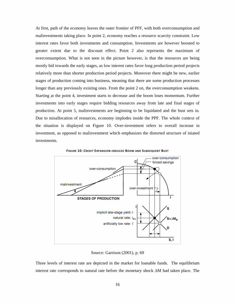
At first, path of the economy leaves the outer frontier of PFF, with both overconsumption and

malinvestments taking place. In point 2, economy reaches a resource scarcity constraint. Low

interest rates favor both investments and consumption. Investments are however boosted to

greater extent due to the discount effect. Point 2 also represents the maximum of

overconsumption. What is not seen in the picture however, is that the resources are being

mostly bid towards the early stages, as low interest rates favor long production period projects

relatively more than shorter production period projects. Moreover there might be new, earlier

stages of production coming into business, meaning that there are some production processes

longer than any previously existing ones. From the point 2 on, the overconsumption weakens.

Starting at the point 4, investment starts to decrease and the boom loses momentum. Further

investments into early stages require bidding resources away from late and final stages of

production. At point 5, malinvestments are beginning to be liquidated and the bust sets in.

Due to misallocation of resources, economy implodes inside the PPF. The whole context of

the situation is displayed on Figure 10. Over-investment refers to overall increase in

investment, as opposed to malinvestment which emphasizes the distorted structure of iniated

investments.

FIGURE 10: CREDIT EXPANSION-INDUCED BOOM AND SUBSEQUENT BUST

Source: Garrison (2001), p. 69

Three levels of interest rate are depicted in the market for loanable funds. The equilibrium

interest rate corresponds to natural rate before the monetary shock ∆M had taken place. The

17

“artificially low rate” is a result of the monetary shock, and corresponds to the combination of

consumption and saving that would support the investment increases from savings, without

the monetary shock. The “implicit late-stage yield” corresponds to a situation when the level

of consumption seen in the boom were not financed by a monetary shock in the form of credit

expansion, but by fall in savings and therefore lower levels of investment.

2.6 INTEREST RATES

Interest rates coordinate time preferences of economic agents with the structure of production.

It coordinates individual plans; plans of consumers to save and consume with plans

entrepreneurs to invest into production. The coordination is inter-temporal; it guides

allocation resources across the structure of production in order to satisfy consumer

preferences reflected in decisions to save and consume. If the interest rates with their

coordination function are distorted, intertemporal equilibrium is upset and the structure of

relative prices becomes distorted. A temporary inconsistency of plans arises, which is

revealed and followed by a costly correction –recession or a depression.

For the sake of simplicity, we focus on distinction between the natural interest rate, i.e. one

that corresponds to equilibrium in the markets for loanable funds, and the actual rate (also

referred to as money rate or loan rate) that temporarily diverges from natural rate as a result of

monetary shock. If the monetary shock is positive, which is the key scenario of ABCT, the

actual rate temporarily diverges downwards.

There have been three main components identified in literature: pure interest rate,

entrepreneurial component and the price component. The fourth that could be added is a

terms-of-trade component, which reflects an accounting distortion that arises from

asymmetric impact of inflation on costs and revenues.5 Pure interest rate (also called originary

interest rate), the one we are most concerned with in the present discussion, reflects solely

time preferences. Mises (2006) explains:

“Time preference manifests itself in the phenomenon of originary interest, i.e., the discount of

future goods as against present goods…Originary interest is a category of human action. It is

operative in any valuation of external things and can never disappear.” (p. 527)

The entrepreneurial component reflects uncertainty and can be seen as synonymous to risk

premium. The price component reflects expectations about future prices. Under stable prices

5 See Rothbard (2008), p.792-798

18

and risk-free world, interest rates prevalent in the market for loanable funds would be equal to

the pure interest rate.

2.6.1 MAG NIT UDE OF INTE RE S T RATE S

In the ABCT, there is a downward divergence of the actual interest rate from the natural rate.

It is important to note that in order for the actual interest rate to diverge from the natural rate,

the actual rate doesn’t necessarily need to rise. If, for example, the natural rate increases

because of expected inflation, increased time preferences or for any other reason, credit

expansion can take place without lowering the actual interest rates, because the natural

interest rate has also been lowered. What is important is the relative movement of the natural

and the actual interest rate. Thus, there can be a divergence of natural rate and the money rate

of interest without the downward movement of the actual interest rates. Rothabrd (1963)

writes:

“To “refute” the Austrian theory of the inception of the boom because interest rates might not

have been lowered in a certain instance, for example, is beside the mark. It simply means that

other forces -perhaps an increase in risk, perhaps expectation of rising prices -were strong

enough to raise interest rates.” (p. 85)

By such standard however, it is problematic not only to refute, but also to confirm the theory.

Just as upward pressures on the interest rates caused by expectations of rising prices or

increase in risk could be strong enough to off-set the downward pressures caused by the credit

expansion, there could be decrease in risk or expectations of lower prices pushing the rate

downward in the absence of the credit expansion-induced boom. Thus, in the absence of

reliable measures of what the natural interest rate is, development of the magnitude of actual

interest rate doesn’t provide a straightforward indication in favor or against the ABCT. When

we talk about decrease in interest rates due to increased savings or due to credit expansion, as

we have when explaining the theory, what we mean is a decrease of the actual rate of interest

relative to the natural rate of interest. Magnitude of the actual rate of interest is not decisive.

There is however a more reliable indication: the liquidity effect.

2.6.2 LI QUI DITY EFF E C T

If the change in interest rates results from a monetary shock rather than falling time

preferences, change in risk conditions or price expectations, a liquidity effect should occur.

This means that the monetary expansion should push the short-term interest rates down to

19

greater extent than the long-term rates, thus making yield curve steeper. The ability of

monetary policy to influence short-term interest rates to greater extent than the long-term

interest rates was explained for example by Romer (2006, p. 503-504). Empirical evidence in

favor of the liquidity effect was put forward by Bernanke and Mihov (1988). Keeler (2001)

used presence of the liquidity effect in empirical data to determine whether interest rates were

affected by a monetary shock. He did so by observing changes in slope of yield curves

throughout eight business cycles in the US economy between 1954 and 1951. The pattern that

would suggest monetary expansion-induced boom includes steep yield curve followed by the

boom, and later transitioning itself into flatter yield curve towards the end of the boom phase

followed by a restructuring phase -recession. We will examine this phenomenon in the

empirical part further below.

2.7 RELATIVE PRICES THROUGHOUT THE BUSINESS CYCLE

In the explanation of the business cycle mechanism, we didn’t fully explain the mechanics of

change behind restructuring of the structure of production. Aim of the following section is to

explain those.

A useful distinction of producer’s goods was coined by von Wieser and later adopted by

Hayek. It is a distinction between specific and non-specific producer’s goods. Specific

producer’s goods enter the production process at some particular stage, or at least at no more

than a few particular stages. They are to large extent fixed to the stage of production they

were designed for and the possibility of their reallocation along the structure of production

according to changes in relative prices is limited. Examples include specialized machinery or

facilities that would lose much of their value upon being employed for some other purpose.

Other examples include materials that require specific processing before they can be passed

further along the production structure. Non-specific producer’s goods on the other hand can

be used at all or many stages of production. Hayek also treated labor and land as non-specific

inputs, although it should be noted that labor itself could be divided into more and less

specific. Hayek referred to labor and land as original means of production. Another example

of nonspecific producer’s goods would be raw materials that require little or no processing

before they can be allocated to different stages of production.

The important feature of the specific vs. non-specific distinction is different extent to which

particular producer’s goods are exposed to competition. Supply of the non-specific producer’s

goods can be competed for by businesses from across the entire structure of production. If

20

products made at some particular stage of production become more expensive to those made

at other stages, the businesses that produce them can bid up the price of the non-specific

inputs and expand, leaving businesses at other stages of production with less and/or more

expensive input resources. Specific producer’s good however, are tied to technology of a

narrow range of production structure and are subject to competition of businesses to lesser

extent than the non-specific producer goods. Furthermore, if specific producer goods at some

particular stage of production are not combined with the needed non-specific producer goods

(complementarity of inputs), they become less productive and their price decreases. As a

result of changing relative prices, the non-specific producer goods move across the stages of

production even in relatively short term, whereas the specific goods first become priced

differently by the markets before their produced quantity changes.

2.7.1 DYNAMIC S OF THE STR UC T URE OF PRICE S

Let’s now focus on the mechanism through which a fall in interest rates is translated into

prolonging of the production structure. If more funds are available for investments, either

from savings or from credit expansion unsupported by savings, this change to the structure of

production manifests itself by increased investments. Under unchanged total income, the area

of the triangle remains the same if investment boom results from increase in savings. In other

words, the economy’s potential has increased and the actual growth followed. If the

investment boom followed a positive monetary shock, the area of Hayekian triangle

temporarily increases as consumption increases. Put differently, the economy grows at a rate

higher than its potential. As the change is not supported by the rise in savings, the hypotenuse

of Hayekian triangle “is broken” and does not have a constant slope (Figure 8). Consumption

does not have to decrease in order to build up more savings. Thus, under a monetary shock-

induced boom, both consumer and producer boom industries can expand at the same time. As

a result of the discount effect, profitability increases to greater extent at early stages of

production. The price increase reflects higher bidding for inputs at the earlier stages, as

depressed interest rates has a higher effect of profitability at early stages. Price changes serve

as a signal for resource reallocation. Prices of producer goods rise relative to prices of

consumer goods, as due to discount effect the early stages are favored to greater extent. An

exception to this overall tendency might be caused by a temporary increase in demand for

consumer goods caused by the overconsumption, which occurs early in the boom (Figure 9).

Similarly, prices of producer goods at earlier stages of production rise relative to prices of

21

products at later stages of production, and new previously unprofitable stages of production

enter the production structure (lengthening of the structure of production).

Hayek used a diagram (Figure 11) to illustrate the impact of changed interest rates on the

structure of production. The five graphs next to each other represent 5 stages of production,

starting with the earliest on the left and the latest on the right.

FIGURE 11: DISCOUNTED MARGINAL PRODUCT ALONG THE STRUCTURE OF PRODUCTION

Source: Hayek (1935), p.80

Curves on each graph represent discounted marginal product of capital (i.e. producer goods)

at a particular stage, measured by the market price at which it can be sold. Shapes of the

marginal productivity curves are identical for each stage. Discounting product at each stage

means a downward shift of the marginal productivity curve and at the same time slightly

changing its slope, as discounting product returned from various invested quantities is not

merely a downward shift, but lowering the undiscounted product by a certain percentage.

There are two discount curves; solid and dotted. The solid curve corresponds to a higher

discount rate and thus assumes a steeper shape. The dotted curve corresponds to a lower

discount rate. Besides the two discount curves, there are two horizontal lines. The one

positioned at the lower level intersects each discounted marginal productivity curve at the

point that marks amount of capital invested under the higher discount rate equilibrium. The

horizontal line positioned at the higher level corresponds to the lower discount rate

equilibrium amount of capital. The equilibrium quantities for each stage are represented with

the distance between intersection of discounted marginal productivity curve and the horizontal

line. The earliest stage is not invested into at all under the higher discount rate. The product

of the latest stage on the very right, where consumer goods are produced is not discounted at

all. A retail store or an online shop with home delivery is a good example of the latest stage,

as no significant amount of time needs to elapse between sale of a product at this stage and its

consumption. When the discount curve shifts from the solid to the dotted as result of

22

depressed interest rates (and hence discount rate), differentials between discounted marginal

products at different stages arise. Prices of products increase most for the earliest stage and

least for the latest stage.

Capital is allocated until the price differentials disappear. Relatively most new investments

occur in the earliest stage that was not in business under the higher discount rate at all. The

second biggest increase occurs in the second earliest stage and so forth. The diagram shows a

fall of invested resources in the late stages. This is the case when under constant income

savings increase and consumption fall. When the fall in interest rates arises from credit

expansion unsupported by savings, there doesn’t have to be any decrease at any stage, only

increase for all stages, but relatively higher for earlier stages of production.

Price changes of producer goods which are products of different stages also depend of the

specificity of the producer good and the marginal productivity, i.e. technology at a particular

stage. These two dimensions are abstracted from in the diagram. Hayek (1935) sums them up:

“The price of a factor which can be used in most early stages and whose marginal

productivity there falls very slowly will rise more in consequence of a fall in the rate of

interest than the price of a factor which can only be used in relatively lower stages of

reproduction or whose marginal productivity in the earlier stages falls very rapidly.” (p.83)

Considerations in this chapter have implications about development of relative prices. With

inception of a credit expansion, there should be a boom with prices development described

above. Input prices at earlier stages of production should be rising relative to those at lower

stages. The earlier a particular stage is positioned in the structure of production the higher

relative growth of input prices it should experience. Industries positioned at earlier stages

should see prices of labor increasing at higher pace as industries positioned at later stages.

Thus, there should be an asymmetric wage growth across the structure of production. Price

changes guide allocation of resources. Thus, industries at early stages should expand more

robustly in the expansion phase of the business cycle.

When the expansion phase comes to an end, a reversal of previous trends should occur.

Distortions created by the credit expansion unsupported by savings should see a correction.

Correction includes a costly abandonment or reduction of production capacities. Industries at

early stages, those that expanded the most, should experience a sharper contraction. Relative

prices should move in the opposite direction. Price differentials that widened in favor of the

early stages of production should be narrowed or eliminated.

23

2.8 EXPECTATIONS AND THE ABCT

2.8.1 THE CRITI QUE

The argument most often brought up in opposition to the ABCT comes from rational

expectation perspective. Supposing that the business cycle follows scenario described by the

theory, why would the theory itself not become a factor in decision making of the business

community? Why can’t the businessmen recognize the policy-induced boom, and adjust their

calculation of the expected profitability of their projects? Moreover, fluctuations in economic

activity appears periodically, so the businessmen can experience it, learn and act accordingly.

Furthermore, the rational expectations objection is not limited to the demand side of the credit

market, i.e. the entrepreneurs. The supply side -the banks, also suffers losses when the boom

ends and loan defaults occur. Had the banks been more conservative in the boom phase and

not participated in the credit expansion (or participated to lesser extent), they could escape the

painful liquidation of debt. The objection from the supply side point of view was also brought

up by Hayek (1933):

“A theory which has to call upon the dues ex machine of a false steps by bankers, in order to

reach its conclusions is, inevitably suspect.” (p. 145)

Tullock (1987) is especially concerned about the repetition of mistakes by the decision

makers implied by the ABCT. He is willing to concede a one-off fooling of the entrepreneurs

by low interest rates. In his comments on Rothbard’s exposition of the theory, Tullock (1987)

states:

“That they [entrepreneurs] would continue unable to figure this out, however, seems

unlikely. Normally, Rothbard and the other Austrians argue that entrepreneurs are well

informed and make correct judgments.” (p. 73)

Wagner (2000) is also suspicious of ABCT’s implication that both the policy-induced credit

expansion as well as the market fundamentals-induced expansion should be met with the same

response by the business planners. He further thinks that even if that could have been an

accurate description of reality in the first half beginning of 20th century, things have changed a

lot ever since:

The central bank’s expansion of credit is treated as indistinguishable from a general increase

in the desire to save. Both instances arrive as surprises, and the two types of surprise are

24

indistinguishable from one another. This situation might have had plausibility when Austrian

cycle theory was initially formulated The collection of economic statistics was

primitive…There was no developed community of financial observers and Fed watchers.

Throughout the postwar period, however, we have become ever increasingly removed from

that earlier time. Statistics, observers, and pundits are everywhere.”(Wagner 2000, p. 14)

Caplan (1997) also rejects the idea of entrepreneurs failing to detect distortions in the market

for loanable funds, especially as they have clear motivation to research the situation and

improve the decision making:

“Given that interest rates are artificially and unsustainably low, why would any businessman

make his profitability calculations based on the assumption that the low interest rates will

prevail indefinitely? No, what would happen is that entrepreneurs would realize that interest

rates are only temporarily low, and take this into account.”6

Responses to the outlined critique come from multiple authors. Generally, they could be

divided into two groups with respect to their approach. The first approach is an application of

the game theory with a conclusion that the expectations are irrelevant; even if they are formed

correctly, decision makers are placed into a prisoner’s dilemma setup which doesn’t change

their decision to participate in the boom. The other approach concedes importance of

expectations. It is founded in insights into accessibility and availability of the kind of

knowledge that could be used to prevent the business cycle.

2.8.2 PRI S ONER ’S DIL E MMA A ND IRRE L E V A NC E OF KNO WL ED GE

One of the possible responses to the objections stated above is to apply game theory, namely

the prisoner’s dilemma.7 This response is a very specific one; it postulates that the knowledge

about mechanisms that generate business cycles is irrelevant and will not change business

decisions so as to avoid the recession.

Carilli and Dempster (2001) build up their prisoner’s dilemma argument by comparing the

hypothetical system of free banking with the system of the banking sector cartelized under the

central bank coupled with monopolized currency issue. The difference that is relevant for the

discussion is a common pool problem that arises from monopoly currency. When banks issue

6 See internet sources list at the end of the paper 7 “The prisoner’s dilemma occurs when the incentive structure is such that the individuals involved in the decision process choose to make decisions that will leave them, collectively, worse off than if each had made a different choice.” (Carilli and Dempster 2001, p. 322)

25

their own money (or money certificates such as cheques, demand deposits etc.), they can

differentiate from other banks by their policy regarding the issue; they can appeal to clients by

being more conservative (keeping higher reserve ratio), and can decide on compatibility with

other banks (transacting other bank’s money with their own clients’ accounts) based on

trustworthiness of other banks’ issue policies. Thus, each bank bears consequences of their

policy, and there is a competition among banks.

When the currency is monopolized however, there is a common pool problem: a single bank

can reap benefits of loose credit policy (keep low reserve ratio, grant more loans and collect

more interest revenue), and at the same time offload the costs of their policy, namely the

liquidity risk, on the entire banking sector. If a bank faces increased demand for credit without

any change in genuine savings, a conservative response (preserving the current reserve ratios)

would be to increase the interest rate. Under common pool monopoly money where banks

share the risks, lowering the reserve ratio is a profit-maximizing strategy. Further elaboration

of this point would be to consider an agreement among banks to be jointly conservative. In

that case however, every single bank has an incentive to break the agreement and undercut

interest rates of other banks; a usual game theory conclusion about cartel instability. Thus, if

we grant that the bankers are familiar with the ABCT and believe it to be correct, game theory

provides an explanation of them taking part in the expansionary lending nevertheless.

We have looked at the supply side of the credit market. If the malinvestment generating credit

expansion is to take place, there must also be willing borrowers, namely business people with

their projects in need of financing. If we concede that the business people correctly determine

that the fall in interest rates is not due to increased savings, but due to credit expansion and

they believe the ABCT to be correct, can the unsustainable investment pattern still emerge?

Prisoner’s dilemma can be applied again. If all the business decision makers refrain from

partaking on projects that would not be expected to generate profit under the natural rate of

interest, the boom-bust cycle could be avoided. For a single firm however, cheaper financing

is a valuable opportunity that should be taken advantage of. In addition to that, any single firm

has no control over other firms’ actions. Thus, the case is similar for supply side and demand

side alike. Garrison (1989) uses following parallel:

“Macroeconomic irrationality does not imply individual irrationality. An individual can

rationally choose to initiate or perpetuate a chain letter—sending one dollar to the person on

26

the top of the list, adding his name to the bottom, and mailing the letter to a dozen other

individuals—even though he knows that the pyramiding is ultimately unsustainable.” (p. 10)

Furthermore, a firm that would like to abstain in taking part in the boom would still have to

compete with those that take part. Such firm would find itself in a position whereas input

resources would be more and more scarce due to demand from businesses that took advantage

of the cheaper credit.

Another point raised by Stanley (2007) pertains to the opportunity costs. If a company passes

on opportunities of cheap credit, it not only cedes market share to competition, but it suffers

from the diminished opportunity costs (i.e. from expected returns from alternatives being

driven down). The risk-free rate declines, and further pressure to participate in the boom is

placed upon the decision-makers.

An important element of knowingly participating in unsustainable boom is timing. Decision

makers do so hoping (or believing) that they would be able to exit before boom turns into

bust. If an investments are exited before any problems become apparent, one can participate

in the boom and avoid bearing the losses. Block (2001) draws on this point:

“The trick, of course, is to get the timing right: to get in while the getting is good, and to

leave someone else holding the bag right before the onset of the downturn in the Austrian

business cycle. But as long as expectations are not perfect and uniform, there is no reason

such a scenario cannot obtain.” (p.66)

This reasoning seems plausible; there is a vast diversity in future forecasts and, more

importantly, very few predictions of economic downturns that turn out correct ex post. This

argument however marks departure from assuming rational expectations, and leads to

discussion of limits of knowledge and possibility of correct expectations, which is another

response to the rational expectations objection directed at ABCT.

2.8.3 LIMI TS OF KNOW LE DGE A ND T HE PO SSI B IL ITY OF CORRE CT EXP E C TATI ONS

We will now look at the rational expectations objection to the ABCT from a different angle.

We shall explore reasons for which, given the ABCT is correct, the decision makers fail to

use it in their planning or fail at applying it in a way conducive to avoiding the boom-bust

cycle.

When evaluating ABCT as a useful tool for business decision making, it is important to

remember the qualitative nature of the theory (as opposed to quantitative). The theory is

27

deductive. It postulates that if the interest rates were pushed bellow their natural level, the

investment projects would be undertaken that under the natural interest rate (one that that

appears under equilibrium in the market for loanable funds) wouldn’t be deemed profitable.

One can deduce the conclusion that the prevailing rate is above or below the natural rate by

exploring the nature of interventions in the credit market. These are the qualitative

considerations.

But is it plausible to expect accurate evaluations on how much the prevailing rates differ

from the hypothetical natural rate? Natural rate is a theoretical rate. Such correctly calculated

magnitude of deviation (quantitative considerations) might help businesses adjust their

planning and thus avoid malinvestments. But interest rate is a price prevailing in the credit

market. If a price of any commodity is fixed bellow (or above for that matter), it’s free-market

level is hard, if not impossible, to determine. These considerations border on the debate over

possibility of calculation in a centrally planned economy, which largely consist of trying to

administratively mimic market prices.8 Theoretical prices which the free market would yield,

the prices that are a result of supply, demand and all the determinants thereof, cannot be

calculated in their absence. Thus the magnitude by which the prevailing interest rates differ

from those undistorted by the monetary policy is impossible to determine. In turn, business

decisions cannot be adjusted accordingly. To use a parallel, “knowing that a signal is jammed

is not the same as knowing what the unjammed signal is.” (Garrison 1986, p. 446)

If businessmen attempted to study places and periods with free market in banking in order to

shed some light on the magnitudes of interest rates under different scenarios, they would find

such periods missing in the modern history. Credit market is a segment notorious for

government intervention. Murphy and Erickson (2005) observe that the major countries have

institutionalized permanent intervention, mostly by establishing central bank and

monopolizing the provision of money supply. That makes successful inquiry into what the

rates could be in absence of such interference even more unrealistic.

Distortion of interest rates also leads to changes in the entire structure of relative prices. These

changes are even more non-traceable. If, for example, a price of commodity X increases by a

particular proportion, there is no way to break down the total change into (i) the impact of

monetary shock and (ii) the changes resulting from market fundamentals, as new money has

an asymmetric impact on prices. Attempts to single out the most significant fundamental

8 See debate on “market socialism” put forward by Oscar Lange and its criticism by FA Hayek

28

determinants of market price, statistically determine magnitudes of their impact on market

prices (based on past data) and claim the residual change in magnitude to be the impact of the

monetary policy would rely wholly on existence of constant relations between statistical

aggregates, which is in itself a problematic proposal.

Hayek’s two kinds of knowledge

In the discussion over nature of knowledge, possibility of aggregating it and making use of it

to centrally plan the economy, Hayek (1945) made a distinction between two kinds of

knowledge. This distinction will serve us as a useful framework in the discussion of

expectations in ABCT. The distinction is as follows:

1) Knowledge of particular circumstances of time and space

2) Scientific knowledge (knowledge about structure of the economy)

The first kind of knowledge is decentralized and arises from a particular activity. If a

businessperson discovers a one-off possibility to purchase some inputs at lower price, they

take advantage without attempting to explain causes of the situation at hand. If demand for the

product rises without any obvious cause, the business person will use up more of existing

capacities and consider expansion long-term, even if the causal chain that led to the situation

escapes their understanding. Existence of this kind of knowledge, as conveyed in price

signals, is the kind of knowledge that led Hayek and Mises to the conclusion of impossibility

of calculation or, more precisely, impossibility of substituting markets by administration in

designing the constantly changing array of relative prices. It is the kind of knowledge specific

to particular business operations which entrepreneurs can reasonably be expected to have.

Scientific knowledge is knowledge about the structure of the economy. This knowledge is

subject to the inquiries of economics as a branch of science. One of the issues that economics

deal with, is the business cycle theorizing. Yet professional economists are far from

agreement over what causes the business fluctuations (Block and Barnett 2005). We cannot

conclude that the conclusive scientific knowledge about the causes of business cycles is held

even by the people who professionally research the subject. Critique that asserts such elusive

knowledge should be used in business planning across the economy thus rests on unrealistic

assumptions. Scientific knowledge, that is knowledge of the structure of economy that is not

generally agreed upon even among economists, cannot be reasonably expected to be

incorporated into decision making across the economy.

29

3 APPLICATION: US ECONOMY 2001- 2009

Callahan and Garrison (2003) as have examined possibilities of explanation of the Dot-Com

boom and bust by the ABCT in the US Economy. Callahan and Garrison focus on

circumstances that lead to channeling of newly created credit into the Dot.com companies and

technological start-ups. Empirical studies of ABCT with praxeological approach include

Rothbard (2008) and Robbins (1934). In both cases, the cycle is treated as a unique

phenomenon with focus on qualitative rather that quantitative grasp of the period. Both works

use ABCT to interpret the Great Depression and preceding boom of the 1920’s. Empirical

works on ABCT with more quantitative approach include Wainhouse (1984), Le Roux (1999)

and Keeler (2001). Wainhouse (1984) derives propositions from ABCT and tests them on the

Great Depression data. Le Roux draws on Wainhouse, applying the same propositions on the

South African business cycle of 1980-1996. Fidings of both Wainhouse and Le Roux are

favorable towards ABCT. Keeler (2001) derives propositions regarding interest rates

development, sectoral capacity utilization and money supply. The propositions are then tested

on 8 business cycles between 1950 and 1991 with largely favorable results, complemented

with discussion of differences across the cycles.

3.1 PROPOSITIONS

In the present paper, we start with a brief macroeconomic description of the period so as to

provide context for further analysis. We will then proceed to apply theory on economic data

from the period. The examined period starts in November 2001, an official end of the

previous recession as announced by the National Bureau for Economic Research. The

examined period ends at the end of 2009, 6 months after NBER announced end of the

recession in June 2009. We shall focus on the sharp downswing and the preceding

expansionary period. The Recovery, outlook and all the related issues are beyond the scope of

this paper. Our analysis will be structured into three major segments. The first segment aims

to establish that the disequilibrium in the market for loanable funds took place, setting stage

for the business cycle mechanism postulated by the ABCT. Two propositions are derived

from the theory and confronted with data under the first segment. The second segment focuses

on sectoral patterns and labor market throughout the boom and bust, with support from three

propositions. Another three propositions regarding development of relative prices are

examined in the third segment. To provide further context, the 8 propositions are

30

complemented with insights to relevant events that took place throughout the period.

Propositions 1,5,6,7 and 8 draw on Wainhouse (1984) and Le Roux (1999), with deviations in

both wording and approach to their verification. Proposition 2 draws on Keeler (2001).

Proposition 3 is a frequently drawn implication of the ABCT and occurs repeatedly in

writings on the subject. Proposition 4 was briefly mentioned as an observation in Rothbard

(2008) without any detailed verification. List of the 8 propositions follows:

Credit Expansion and the Market for Loanable Funds

• Proposition 1: Changes in the supply of savings are independent of changes in the

supply of bank credit, enabling disequilibrium in the market for loanable funds.

• Proposition 2: Liquidity effect, an indication of the monetary shock, takes place as

result of a monetary shock

Sectoral Patterns and the Labor Market

• Proposition 3: Credit expansion stimulates industrial activity at earlier stages of

production to greater extent than at later stages of production

• Proposition 4: Wages at earlier stages of production grow at higher rate than wages at

later stages of production during the expansion period of the cycle.

• Proposition 5: At the end of the upswing, unemployment should increase first and with

greater intensity in industries at early stages of production, and with some lag and

lesser intensity in industries at later stages.

Relative Prices

• Proposition 6: The ratio of producer prices to consumer prices tends to rise after the

initiation of a credit expansion.

• Proposition 7: During the expansion phase, prices of producer goods closest to final

consumption tend to decline relative to the prices of producer goods further away from

the later stages of production.

• Proposition 8: The prices of consumer goods rise relative to the prices of producer

goods, reversing the initial shift in relative prices as credit is contracted towards the

end of the cycle. Similarly, prices of producer goods at later stages will rise relative to

prices of producer goods at earlier stages.

31

3.2 MACROECONOMIC DESCRIPTION OF THE PERIOD

Description of the macroeconomic development during the examined period will provide

context for application of the theory. If not stated otherwise, data used in the text were

obtained from the Federal Reserve Economic Data (FRED) or annual reports of the Board of

Governors of the Federal Reserve System from 2001-2009.

3.2.1 GR OS S DO ME STI C PR OD UC T

GDP growth remained humble throughout 2002. It started to pick up early in 2003, following

FOMC’s reduction of Fed funds rate from 1.75% to 1.25% in November 2002, resulting in

equity market rally as well as increased demand for mortgages. Industrial production and

investor confidence started to turn up in the second half of 2003. By the end of 2003, the real

annual GDP growth rate spiked from around 2% to nearly 4%.

FIGURE 12: US REAL GDP ANNUAL GROWTH

After a slight decrease to 3%, the growth remained steady and lasted until mid 2006, marking

a strong and long expansionary period. The economy was deemed to be in a good shape:

“Over the course of the spring, it became clearer that the expansion was solidifying.

Businesses added appreciably to their payrolls, boosted investment in equipment and

software, and started restocking inventories. While household spending growth softened

somewhat, residential construction expanded rapidly.” (Fed Board of Governors 2004, p. 3)

In 2005, real GDP grew at 3%, with growth slowing down in the 4th quarter as a consequence

of damage inflicted by a series of hurricanes in the Mexican Gulf, most notably Katrina.

32

Household spending grew stronger compared to 2004. The development was largely ascribed

to the wealth effect rather than income effect:

“The rapid gain in real estate values in the past few years, in combination with the rise in

stock prices since 2002, has encouraged households to sustain their spending through a

period of relatively weak growth in real income.” (Fed Board of Governors 2005, p. 3)

Economic expansion as measured by the GDP growth slowed down slightly in 2006, but

gained momentum in the first half of 2007. Growth decelerated sharply in 2007 and GDP

began to contract in the second quarter of 2008. Annual GDP growth remained negative until

the end of 2009.

The second half of 2008 and early 2009 were periods of severe strain in the financial sector,

resulting in failures of several major institutions. In March 2008, Bear Stearns experienced a

liquidity crisis that led to its acquisition by JP Morgan Chase & Co. Similarly, acquisition of

Merryll Lynch by Bank of America was announced in September 2008 and took place in

January 2009. On September 15 2008, Lehman Brothers filed for bankruptcy. In October of

the same year, acquisition of distressed Wachovia by Wells Fargo was announced. Other

notable bankruptcies include the Indy-Mac Federal Bank in July and Washington Mutual in

September 2008.

3.2.2 HOUSING MARKET

The housing market peaked early in 2006 after a long and sustained growth, and declined

slightly throughout 2006. Gains in homeowner’s equity were a major source of consumer

spending, as soaring home equity values created wealth effect and served as collateral for

consumer spending. Rising prices of real-estate, equities and commodities were cited by

FOMC as a reason for the Fed funds rate increases and viewed as potential CPI inflationary

pressures. A slowdown in construction sector as a result of mild correction of prices in 2006

was perceived as a warning sign by the few:

“Although the contraction in homebuilding has been a drag on growth, that restraint seems

likely to diminish over 2007.” (Fed Board of Governors 2006, p. 3)

In the second half of 2006, residential construction continued to plunge. Moreover, a

slowdown in the car manufacturing sector occurred. However, consumer spending and

employment were still growing. Throughout 2007, housing market was rapidly plummeting

after the years of booming:

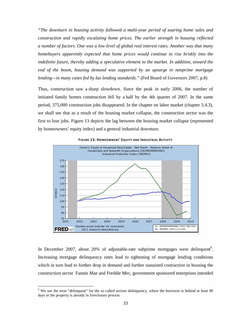
33

“The downturn in housing activity followed a multi-year period of soaring home sales and

construction and rapidly escalating home prices. The earlier strength in housing reflected

a number of factors. One was a low level of global real interest rates. Another was that many

homebuyers apparently expected that home prices would continue to rise briskly into the

indefinite future, thereby adding a speculative element to the market. In addition, toward the

end of the boom, housing demand was supported by an upsurge in nonprime mortgage

lending—in many cases fed by lax lending standards.” (Fed Board of Governors 2007, p.8)

Thus, construction saw a sharp slowdown. Since the peak in early 2006, the number of

initiated family homes construction fell by a half by the 4th quarter of 2007. In the same

period, 375,000 construction jobs disappeared. In the chapter on labor market (chapter 3.4.3),

we shall see that as a result of the housing market collapse, the construction sector was the

first to lose jobs. Figure 13 depicts the lag between the housing market collapse (represented

by homeowners’ equity index) and a general industrial downturn.

FIGURE 13: HOMEOWNERS' EQUITY AND INDUSTRIAL ACTIVITY

In December 2007, about 20% of adjustable-rate subprime mortgages were delinquent9.

Increasing mortgage delinquency rates lead to tightening of mortgage lending conditions

which in turn lead to further drop in demand and further sustained contraction in housing the

construction sector Fannie Mae and Freddie Mec, government sponsored enterprises intended

9 We use the term “delinquent” for the so called serious delinquency, where the borrower is behind at least 90 days or the property is already in foreclosure process

34

to increase mortgage accessibility and boost home ownership, were suffering from sizeable

losses. Their stocks began to plummet in June 2008. Worries that their capital would be

insufficient to cover losses led the Treasury and the Congress to inject more capital into the

two institutions in July and put them under conservatorship in September 2008. In November

2008, sub-prime mortgage delinquency rate stood at 25%. In December, prime mortgage

delinquency reached 3.75%, having doubled over the last year. 2 million homes entered

foreclosure process in 2008 after 1.5 million in 2007. The number never exceeded 1 million

2003-2006. After the sharp downturn, the housing market didn’t show signs of recovery until

the end of 2009, the end of our examined period.

3.2.3 UNE MPL OYME NT

Payroll employment didn’t start to increase until mid 2003 as a result of investors’ low

confidence and unwillingness to expand and hire. Starting in mid 2003, the expansion in

industrial production led to a long-lasting steady drop in unemployment rate. After the

ambiguous 2003, 2004 saw a clear increase in hiring and considerable drop in the

unemployment rate.

FIGURE 14: UNEMPLOYMENT

In 2005, improvement continued with 2 million new jobs created on the net in the economy.

Despite the signs of a slowdown, first in construction and then in car manufacturing, labor

market remained strong and unemployment rate kept decreasing steadily throughout 2006. At

the end of 2006 and beginning of 2007, unemployment rate remained stagnant close to its

35

bottom at about 4.5%. By the end of 2007, it reached 5%. Unemployment was increasing

sharply throughout 2008. Between December 2007 and January 2009, 3.75m private sector

jobs were lost. Civilian unemployment rate stood at 5% at the beginning of the year and

climbed to nearly 8% by the year’s end. The Fed Board of Governors summarized the

situation as follows:

As of February 2009, manufacturing employment has fallen nearly 500,000 over the past

three months and has dropped more than 1 million since December 2007. Layoffs in truck

transportation and wholesale trade, which are closely related to activity in the manufacturing

sector, show a similar pattern. The decline in construction employment, which began in early

2007, has also sped up, in part because the ongoing contraction in homebuilding has been

accompanied more recently by weakness in nonresidential building. In the service-producing

sector, job losses have mounted at retail establishments, providers of financial services, and

professional and business services firms, all of which have been adversely affected by the

downturn in economic activity. A noticeable exception has been the continued brisk hiring by

providers of health services. (Fed Board of Governors 2007, p.16)

The unemployment rate kept increasing until the end of 2009.

3.2.4 FE DE RAL RE S ER VE ’S POLIC Y A ND M ONE TAR Y DE VE L OP ME NT

2002 was still a year of unconvincing recovery. FOMC decided to keep the Fed funds rate at

1.75%. Further deterioration of the labor market situation prompted a rate cut to 1.25% in

November 2002. Uncertain recovery coupled with the beginning of the war in Iraq led the

FOMC to a decision of keeping the Fed funds rate at low levels at their meetings in March

and May 2003. Moreover, the Fed funds rate was lowered by the FOMC in June by 25 basis

points to 1%. FOMC’s cited concerns about low CPI inflation levels as one of the key reasons

for this policy measure. The exceptionally low Fed fund rates were thought to present no

significant danger as labor productivity growth was expected to keep inflationary pressures in

check.

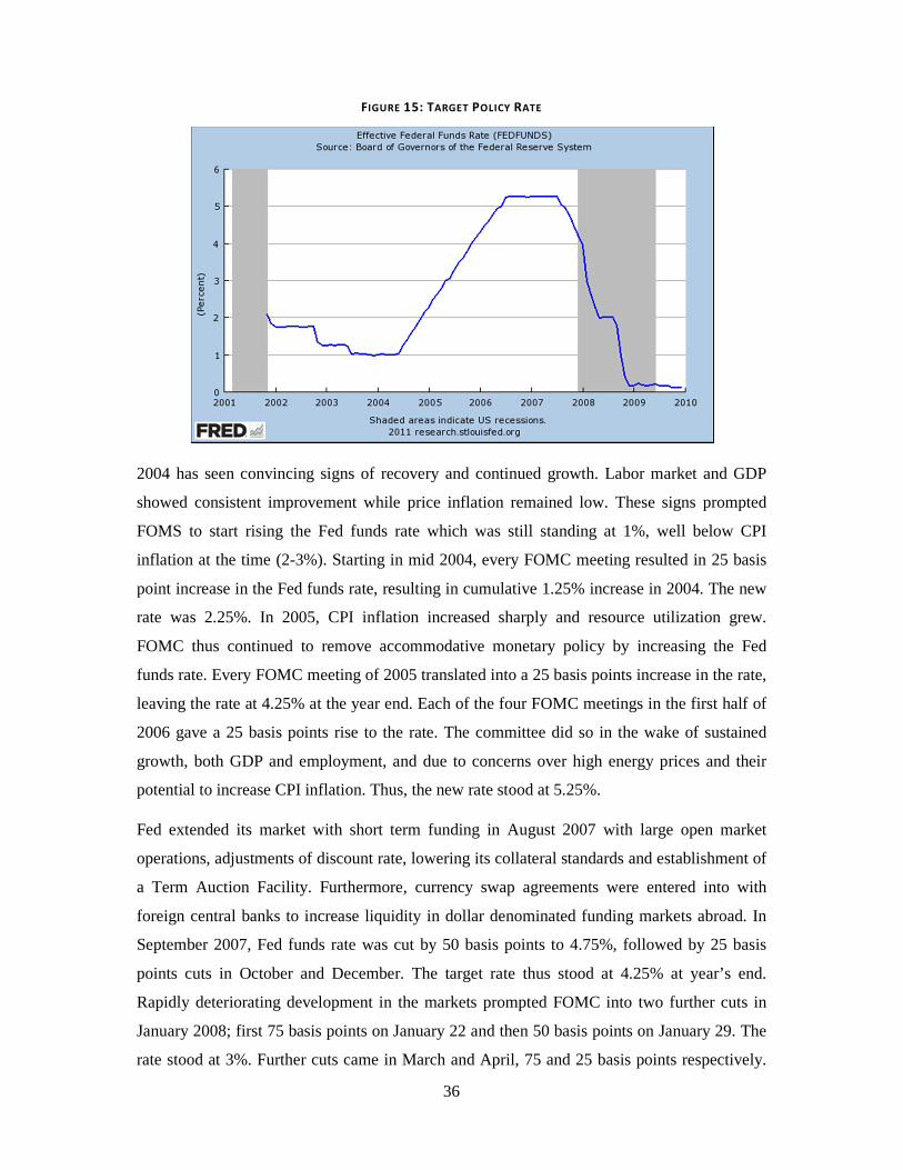
36

FIGURE 15: TARGET POLICY RATE

2004 has seen convincing signs of recovery and continued growth. Labor market and GDP

showed consistent improvement while price inflation remained low. These signs prompted

FOMS to start rising the Fed funds rate which was still standing at 1%, well below CPI

inflation at the time (2-3%). Starting in mid 2004, every FOMC meeting resulted in 25 basis

point increase in the Fed funds rate, resulting in cumulative 1.25% increase in 2004. The new

rate was 2.25%. In 2005, CPI inflation increased sharply and resource utilization grew.

FOMC thus continued to remove accommodative monetary policy by increasing the Fed

funds rate. Every FOMC meeting of 2005 translated into a 25 basis points increase in the rate,

leaving the rate at 4.25% at the year end. Each of the four FOMC meetings in the first half of

2006 gave a 25 basis points rise to the rate. The committee did so in the wake of sustained

growth, both GDP and employment, and due to concerns over high energy prices and their

potential to increase CPI inflation. Thus, the new rate stood at 5.25%.

Fed extended its market with short term funding in August 2007 with large open market

operations, adjustments of discount rate, lowering its collateral standards and establishment of

a Term Auction Facility. Furthermore, currency swap agreements were entered into with

foreign central banks to increase liquidity in dollar denominated funding markets abroad. In

September 2007, Fed funds rate was cut by 50 basis points to 4.75%, followed by 25 basis

points cuts in October and December. The target rate thus stood at 4.25% at year’s end.

Rapidly deteriorating development in the markets prompted FOMC into two further cuts in

January 2008; first 75 basis points on January 22 and then 50 basis points on January 29. The

rate stood at 3%. Further cuts came in March and April, 75 and 25 basis points respectively.

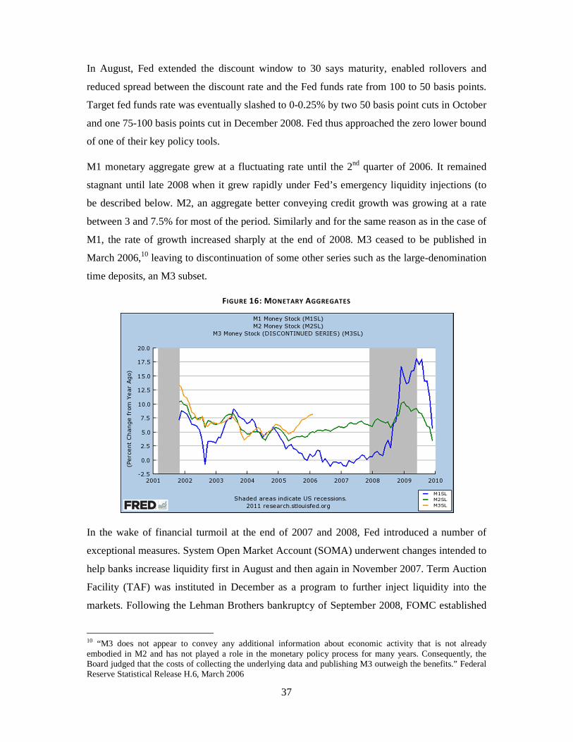
37

In August, Fed extended the discount window to 30 says maturity, enabled rollovers and

reduced spread between the discount rate and the Fed funds rate from 100 to 50 basis points.

Target fed funds rate was eventually slashed to 0-0.25% by two 50 basis point cuts in October

and one 75-100 basis points cut in December 2008. Fed thus approached the zero lower bound

of one of their key policy tools.

M1 monetary aggregate grew at a fluctuating rate until the 2nd quarter of 2006. It remained

stagnant until late 2008 when it grew rapidly under Fed’s emergency liquidity injections (to

be described below. M2, an aggregate better conveying credit growth was growing at a rate

between 3 and 7.5% for most of the period. Similarly and for the same reason as in the case of

M1, the rate of growth increased sharply at the end of 2008. M3 ceased to be published in

March 2006,10 leaving to discontinuation of some other series such as the large-denomination

time deposits, an M3 subset.

FIGURE 16: MONETARY AGGREGATES

In the wake of financial turmoil at the end of 2007 and 2008, Fed introduced a number of

exceptional measures. System Open Market Account (SOMA) underwent changes intended to

help banks increase liquidity first in August and then again in November 2007. Term Auction

Facility (TAF) was instituted in December as a program to further inject liquidity into the

markets. Following the Lehman Brothers bankruptcy of September 2008, FOMC established

10 “M3 does not appear to convey any additional information about economic activity that is not already embodied in M2 and has not played a role in the monetary policy process for many years. Consequently, the Board judged that the costs of collecting the underlying data and publishing M3 outweigh the benefits.” Federal Reserve Statistical Release H.6, March 2006

38

the Asset Backed Commercial Paper Money Market Mutual Fund Liquidity Facility and

Commercial Paper Funding Facility. Money Market Investor Funding Facility was established

in October and Term Asset-Backed Securities Loan Facility in November. Troubled Asset

Relief Program (TARP) was established as a part of the Emergency Economic Stabilization

Act on October 3 2008, leading to Fed purchases of mortgage-backed debt and further

expanding its balance sheet. In November, Fed announced a plan to purchase $100bn in direct

obligations of housing-related government-sponsored enterprises and $500bn in mortgage-

backed securities. The operation was carried out throughout 2009.

FIGURE 17:FEDERAL RESERVE BALANCE SHEET DEVELOPMENT

Source: The Federal Reserve Board of Cleveland

All programs were intended to add liquidity, either by extending credit at emergency

conditions or by accepting assets as collateral that would not have been accepted by the

markets or by outright asset purchases. American International Group (AIG)11, Citigroup and

Bank of America (BoA) were extended special lines of credit, capital injections, guarantees

and special liquidity access facilities throughout the year in order to prevent them from

becoming illiquid. Federal Deposit Insurance Corporation (FDIC) substantially extended its

guarantees under the Temporary Liquidity Guarantee Program.

11 Federal Reserve Board agreed to extend $85bn in emergency loans to AIG on September 16, “In view of the likely spillover effects to other financial institutions of a disorderly failure of AIG and the potential for significant pass-through effects to the broader economy.“ (Fed Board of Governors, 2008)

39

Another area relevant for the discussion is the reserve requirement policy, as it impacts which

the banking sector’s expansionary potential. Throughout the period, required reserve ration

didn’t change. Every depository institution can keep an extension amount on which no

reserves are required. Then there is a low-reserve tranche subject to 3% reserve requirement.

Deposits over the low-tranche amount are subject to 10% reserve requirement.12 Despite the

fact that the reserve ratios were unchanged, effective amount of required reserves can be

changed by changing the exemption amount and the low-reserve tranche amount. These

changes are done at the end of each year, effective for the next year. Impact of the changes on

total required reserves are estimated by the Fed.

FIGURE 18: FED'S RESERVE REQUIREMENTS POLICY ($MILLION)

Exemption Low-reserve Tranche Estimated Impact on

Total Required

Reserves

2001 5.5 42.8 60

2002 5.7 41.3 154

2003 6 42.1 -201

2004 6.6 45.4 -689

2005 7 47.6 -506

2006 7.8 48.3 -369

2007 8.5 45.8 146

2008 9.3 43.9 57

2009 10.3 44.4 -270

Based on Fed Board of Governors data

Changes to the exemption and the low-tranche amount were predominately inflationary. Total

amount of required reserves rose somewhat in 2001 and 2002. Between 2003 and 2006, the

amount of required reserves was decreasing. Most notable decreases came in 2004-2006,

$689m, $506m and $369m respectively. Cumulative cuts of required reserves can be seen in

Figure 19.

12 The low-reserve tranche rate was set to 3% and the exemption amount was introduced under the Garn-St Germain Depository Institutions Act of 1982, the reserve ratio for amount beyond the low-reserve tranche was last change in 1992 from 12% to 10%

40

FIGURE 19: CUMULATIVE CUTS IN TOTAL RESERVE REQUIREMENTS

Based on Fed Board of Governors data

Although the approximately $1.5bn cuts in required reserves is small relative to aggregates

such as total investment and saving (both in thousand of billions), what is important is that the

absolute required reserves were decreasing while the monetary base was steadily increasing.

At the same time, banks were fully loaned up, keeping their voluntary reserve very close to

zero, as displayed by the Figure 20.

FIGURE 20: RESERVES AND MONEY BASE

-500

-

500

1,000

1,500

2,000

2000 2001 2002 2003 2004 2005 2006 2007 2008 2009

Estimated

Cumulative Cuts

in Total Required

Reserves

2001-2009,

$million

41

3.2.5 CO NS U ME R PRIC E INFL ATI ON

Gradual increases in CPI inflation between 2002 and 2005 were mostly caused by rising

energy prices, which in turn were caused by rising prices of crude oil. As price of crude oil

has a big impact on the structure of relative prices, it shall be discussed in a section on relative

prices below. The CPI inflation spiked sharply in 2007, following a further increase in energy

prices. Moreover, food prices saw the largest rise in almost two decades (energy and food

prices will be discussed in more detail in the chapter on relative prices, section 3.5.3).

FIGURE 21: CPI INFLATION

CPI inflation kept accelerating well into 2008 following the commodity boom, in particular

boom of agricultural commodities and crude oil. CPI inflation rate peaked shortly before mid

2008 at 5.5%, then plunged sharply following the collapse of commodity prices.

3.2.6 STOC K MA RK E T

Especially in the first half of 2002, equities plunged after a mild post recession recovery.

Cited reasons include uncertainty about future economic climate due to elevating suspicions

of corporate malpractice after the Enron bankruptcy and concerns about geopolitical situation

in Iraq. The fears of corporate malpractice gradually weakened as no new cases occurred. The

geopolitical concerns nevertheless persisted and grew stronger as civil war in Venezuela

broke out and tensions appeared in Korean Peninsula. The stock market bottomed out early in

2003 and rallied with minor fluctuations until late 2007. Strong gains in stock prices went on

even after the mortgage delinquencies surfaced and investors began to doubt validity of

42

valuations of multiple other asset classes. In turn, instruments backed with asset classes whose

value came into doubt also became suspicious and couldn’t be used as collateral in private

lending market. Liquidity was severely reduced. The Stock market peaked in October 2007.

Since its bottom in February 2003 to the peak, S&P 500 gained 84% in value (average annual

growth of 13.9%) and Dow Jones Industrial Average gained 76% (average annual gains of

12.8%).

FIGURE 22: STOCK MARKET

According to ABCT, monetary shock in the form of credit expansion leads to unsustainable

boom by distorting relative prices and structure of production. Before we proceed to examine

relative prices and sectoral patters throughout the cycle, we need to establish that the

monetary shock had taken place, disequilibriating the market for loanable funds. Due to

additional money in the economy, investments temporarily exceed savings. In order for such

equilibrium to happen, changes in the supply of credit must be independent of the changes in

the supply of savings.

3.3 CREDIT EXPANSION AND THE MARKET FOR LOANABLE FUNDS

In order to examine all the patterns predicted by the theory, we first need to establish that the

prerequisites for the business cycle mechanism postulated by ABCT were in place. In

particular, we need to establish that credit expansion gave rise to unsustainable investment

path by creating disequilibrium in the market loanable funds.

43

3.3.1 INV E STME NT A ND SAVI N G

Disequilibrium in the market for loanable funds is represented by the gap between investment

and saving. The gap can be seen clearly in figure 23. Investment and saving moved together

until early 2004, when they started to diverge. The gap only closed at the beginning of

recession with a sharp decrease in investment coupled with fall in consumption.

FIGURE 23: SAVINGS AND INVESTMENT

Also in line with the theory is the development of the gap with respect to credit growth.

Figure 24 shows gradual build-up of the gap preceded by a sharp increase in the rate of credit

growth. The gap closes and saving outstrips investment after credit growth decelerates.

FIGURE 24: CREDIT EXPANSION AND THE SAVINGS GAP

Based on FRED and Fed Board of Governors data

-2%

0%

2%

4%

6%

8%

10%

12%

-1,500

-1,000

-500

-

500

1,000

Cumulative

Aggregate (I-S),

$bn (left scale)

Annual Credit

Growth,

% (right scale)

44

In order for the gap between savings and investment to occur, credit growth must become

independent of savings.

3.3.2 PR OP OS I TI O N 1: CRE DIT BEC O ME S DE TAC HE D F RO M SAVI N GS

Proposition 1: Changes in the supply of savings are independent of changes in the supply of

bank credit, enabling disequilibrium in the market for loanable funds.

This proposition reflects the discussion of the effects of credit expansion unsupported by

savings, which enables satisfaction of demand in the market for loanable funds to the extent

greater than the available supply of savings. This should manifest itself in banks being able to

grant loans regardless of saving deposits they collect. Thus, an investment pattern divorced

from the time preferences of economic agents can temporarily arise.

The proposition was tested by Le Roux (1999) on South African data. A Granger causality

test can be applied for the test. The idea of the test is to determine whether lagged values of

one variable (up to a particular n-th lag) are useful in determining values of the other variable.

We will do the test both ways. To test the hypothesis, we use FRED monthly data for annual

changes in credit at all commercial banks and for annual changes in aggregate savings

deposits. Figure 25 displays test results.13

FIGURE 25: CAUSALITY BETWEEN CREDIT AND SAVINGS

H0 # of Monthly

Lags

F-statistic P-value

Savings does not Granger-cause Credit 3 1.814 0.153

Credit does not Granger-cause Savings 3 2.355 0.078

Savings does not Granger-cause Credit 5 1.024 0.409

Credit does not Granger-cause Savings 5 1.790 0.124

Based on FRED data

The null hypothesis is absence of causality between credit and savings in both ways. The test

was run taking into account first the last 3 and then the last 5 monthly statistics. On 5%

confidence level, we cannot reject the null hypothesis for either of the tests. With bank growth

credit independent of increases in savings, conditions are set for a disequilibrium in the

market for loanable funds. We thus confirm the proposition 1.

13 See appendix for the regression software outputs

45

3.3.3 PR OP OS I TI O N 2: THE L IQ UIDI TY EFF E C T

Proposition 2: Liquidity effect, a monetary shock indicator, takes place at the beginning of the

expansionary period.

If credit supply increases as a result of monetary policy and not due to changes in market

fundamentals, the interest rate is pushed below its equilibrium or “natural” level. We have

establishes that the difference in magnitude is not a definitive indication, as other causal

forces can exact un upward pressure of interest rates, perhaps outweighing the downward

pressures caused by credit expansion. Furthermore, trying to measure the deviation from the

natural interest rate would leave us with a rather illusive task of devising methods to find out

what the natural rate should be. We will thus not place a great deal of importance on absolute

magnitude of interest rates. Instead, we will turn to a concept of liquidity effect discussed in

the section on interest rates. In order to establish that a monetary shock in the form of credit

expansion has taken place, we shall look for its indicator in the form of liquidity effect.

The liquidity effect can be recognized by observing the development of the slope of the yield

curve. Monetary expansion should depress interest rates across the entire term structure,

however the short term rates should temporarily be depressed to greater extent. So the pattern

we would expect is a temporary increase in slope (=steeper yield curve) as the credit

expansion begins, followed by a decrease in slope as the liquidity effect is only short-term

regardless of continuation of the credit expansion. Keeler (2001) summarizes his findings on

the occurrence of the liquidity effect in 8 business cycles between 1950 and 1991:

“Despite the variation across cycles, a pattern emerges that in the expansion phase, the

short-term rate is low relative to the long-term rate, and late in the expansion and in the

recession, the short-term rate rises relative to the long-term rate.” (Keeler 2001, p. 338)

Thus, we expect the pattern of steep yield curve early in the cycle and then flattening out of

the yield curve either late in the expansion phase or early in recession. We will examine the

yield curve slope development for both private and government debt. For the government

debt, we used monthly data for 10 years constant maturity treasury as a long-term rate and 3

months constant maturity treasury as a short-term rate. For private debt, monthly data for

Bank of America Merryll Lynch 10-15 corporate bonds yield was used as a long-term rate,

and 3 months AA commercial paper rate was used as a short-term rate. Slopes were calculated

using the following formula:

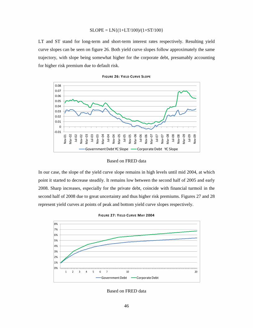
46

SLOPE = LN{(1+LT/100)/(1+ST/100}

LT and ST stand for long-term and short-term interest rates respectively. Resulting yield

curve slopes can be seen on figure 26. Both yield curve slopes follow approximately the same

trajectory, with slope being somewhat higher for the corporate debt, presumably accounting

for higher risk premium due to default risk.

FIGURE 26: YIELD CURVE SLOPE

Based on FRED data

In our case, the slope of the yield curve slope remains in high levels until mid 2004, at which

point it started to decrease steadily. It remains low between the second half of 2005 and early

2008. Sharp increases, especially for the private debt, coincide with financial turmoil in the

second half of 2008 due to great uncertainty and thus higher risk premiums. Figures 27 and 28

represent yield curves at points of peak and bottom yield curve slopes respectively.

FIGURE 27: YIELD CURVE MAY 2004

Based on FRED data

-0.01

0

0.01

0.02

0.03

0.04

0.05

0.06

0.07

0.08

No

v-0

1

Ma

r-0

2

Jul-

02

No

v-0

2

Ma

r-0

3

Jul-

03

No

v-0

3

Ma

r-0

4

Jul-

04

No

v-0

4

Ma

r-0

5

Jul-

05

No

v-0

5

Ma

r-0

6

Jul-

06

No

v-0

6

Ma

r-0

7

Jul-

07

No

v-0

7

Ma

r-0

8

Jul-

08

No

v-0

8

Ma

r-0

9

Jul-

09

No

v-0

9

Government Debt YC Slope Corporate Debt YC Slope

0%

1%

2%

3%

4%

5%

6%

7%

8%

1 2 3 4 5 6 7 10 20

Government Debt Corporate Debt

47

FIGURE 28: YIELD CURVE MARCH 2007

Based on FRED data

The yield curve slope followed the trajectory that corresponds to liquidity effect. Moreover,

with the flattening out of the yield curve, interest rates increased for maturities up to

approximately 7 years. Magnitudes of interest rates changes do not provide conclusive

evidence, as there is no reliable measure of natural interest rates. Development of the yield

curve slope however indicates a liquidity effect which results from a monetary shock.

According to the theory, monetary shock has an impact on term structure of interest rates,

regardless of their observed magnitudes.

3.4 SECTORAL PATTERNS AND THE LABOR MARKET

We shall examine 7 industrial sectors: mining & logging, construction, durable

manufacturing, non-durable manufacturing, utilities, wholesale and retail. What we are

interested in is approximately matching the seven industries with the (temporal) stages of

production. Even every one of the 7 industries is an aggregate that covers a number of sub-

industries and various productive activities. There is no comprehensive data that would match

sectoral activity with temporal distance from delivering the final product. For the purposes of

testing our proposal however, it suffices to arrange the sectors relative to each other, then

examine if the relative impact of credit expansion on activity across the sectors corresponds to

such arrangement.

The two uncontroversial industries are the one closest and the one most distant to delivery of

consumer goods to the end consumer. Retail is generally the last stage of production, through

which consumer goods from other industries make one final step towards the end consumer.

The earliest out of the 7 stages is the mining & logging sector, as it is involved in resource

0%

1%

2%

3%

4%

5%

6%

7%

1 2 3 4 5 6 7 10 20

Government Debt Corporate Debt

48

extraction. Resources are further passed to construction and manufacturing. Thus, in the

spectrum of late-early stages of production, we can expect retail to be a lower bound and

mining & logging to be an upper bound.

Manufacturing is further divided into durables and non-durables. Examination of further sub-

sectoral breakdown reveals that the non-durable manufacturing to a large extent consists of

industries such as foods, beverages textiles and clothing, which are largely channeled through

a small number of further stages to consumer markets. Petroleum and rubber processing are

exceptions from the overall consumer-oriented non-durable manufacturing sector. Durable

manufacturing includes all the material processing except petroleum and rubber, including all

stages of mineral and metal processing. It includes production of all industrial machinery and

equipment, including transportation equipment. Exceptions from the overall producer goods

market orientation of the sector are consumer electronics and furniture manufacturing. We

will thus assume that durable manufacturing sub-sectors are allocated along relatively earlier

stages of production than the non-durable manufacturing subsectors.

Construction sector includes all construction; residential, commercial and industrial.

Construction of commercial and industrial real-estate is a production of producer goods. It

does not directly satisfy consumer demand, instead it produces inputs for production at

different, but relatively later stages. It can include anything from retail mall or office space to

a power plant construction. Construction spending throughout the period of 2002-2009 totaled

$8.926 trillion. Residential construction spending accounted for $3.993 trillion or 44.73% of

total. Non-residential, including commercial and industrial, accounted for $4.933 trillion or

55.27% of total14. Furthermore, only residential units owned and occupied by same agents can

be considered a consumer good, much of them are owned for the purposes of renting them

out, thus using the units as a producer good for service provision. Home ownership rate

during the same period fluctuated between 67.1% and 68.9%, averaging at 68.3%.15 Thus,

about 30.55% of total construction costs were directed at delivering residential units for

consumption purposes. 14.18% produced rental residential units, producer goods at relatively

late stages of production structure, and 55.27% of those costs were directed at producing

producer goods at a wide range of relatively early stages. An important observation about

construction’s position in the structure of production is that most of its non-labor and non-

transportation inputs are supplied by the durable manufacturing; namely industrial machinery

14 FRED database 15 US Census Bureau database

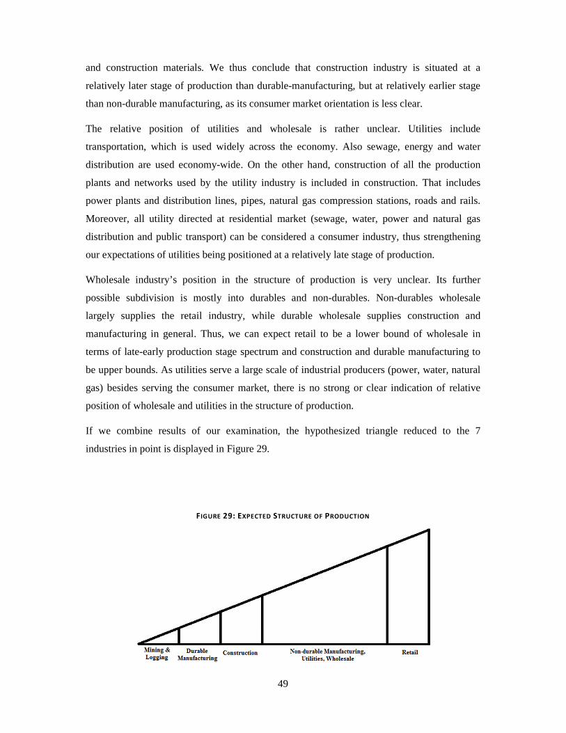
49

and construction materials. We thus conclude that construction industry is situated at a

relatively later stage of production than durable-manufacturing, but at relatively earlier stage

than non-durable manufacturing, as its consumer market orientation is less clear.

The relative position of utilities and wholesale is rather unclear. Utilities include

transportation, which is used widely across the economy. Also sewage, energy and water

distribution are used economy-wide. On the other hand, construction of all the production

plants and networks used by the utility industry is included in construction. That includes

power plants and distribution lines, pipes, natural gas compression stations, roads and rails.

Moreover, all utility directed at residential market (sewage, water, power and natural gas

distribution and public transport) can be considered a consumer industry, thus strengthening

our expectations of utilities being positioned at a relatively late stage of production.

Wholesale industry’s position in the structure of production is very unclear. Its further

possible subdivision is mostly into durables and non-durables. Non-durables wholesale

largely supplies the retail industry, while durable wholesale supplies construction and

manufacturing in general. Thus, we can expect retail to be a lower bound of wholesale in

terms of late-early production stage spectrum and construction and durable manufacturing to

be upper bounds. As utilities serve a large scale of industrial producers (power, water, natural

gas) besides serving the consumer market, there is no strong or clear indication of relative

position of wholesale and utilities in the structure of production.

If we combine results of our examination, the hypothesized triangle reduced to the 7

industries in point is displayed in Figure 29.

FIGURE 29: EXPECTED STRUCTURE OF PRODUCTION

50

The triangle is a simplification. It leaves out industries not included in our analysis. At the

same time, it doesn’t take into account how intertwined subsectors of particular industries are

with each other, which makes strict ordering of the industries across the structure of

production impossible. Some industries will have their subsectors allocated at very differing

stages of production. Those insights are concealed in the statistical aggregates. We will

nevertheless accept the triangle as a useful approximation of general tendencies in the

structure of production with regard to the 7 industries. That will allow us to test the impact of

credit growth on activity and labor market development in industries across the production

structure. As the analysis of the nature of the 7 industries gave us no clear conclusions

regarding order of the non-durable manufacturing, utilities and wholesale, we leave them

unordered and perhaps a subject for future research.

3.4.1 PR OP OS I TI O N 3: IN DUS TRIAL AC TIV ITY A ND THE STRUC T URE O F PR ODUC TI O N

Proposition 3: Credit expansion stimulates industrial activity at earlier stages of production

to greater extent than at later stages of production.

ABCT postulates that credit expansion has an asymmetric impact on industries at various

stages in the structure of production. In the expansion phase, industries whose operations are,

in terms of time, more distant from delivering consumer goods will expand more than the

industries closer to delivery of consumer goods. To measure activity in particular industries,

we have selected monthly data of annual change of employment. An alternative measure of

sectoral activity could be capacity utilization, as suggested by Keeler (2001). Available data

for employment however allow for more detail breakdown of industrial activity. Employment

growth for the 7 sectors is displayed on the figure 30.

51

FIGURE 30: EMPLOYMENT BY SECTORS

In order to determine whether the impact of credit growth on activity was stronger for the

industries at relatively earlier stages than on industries at relatively later stages, we regress the

employment growth data for each sector on credit growth data with a quarterly lag. The

quarterly lag is intended to allow credit flow to take its course and translate into industrial

hiring. In order to account for other influences, we add a general industrial activity index

published by FRED. A test of collinearity between lagged credit growth and industrial index

growth supports inclusion of both variables.16 Other influences include specific circumstances

that lead to exceptionally vigorous pro-cyclical activity in particular sectors. In the 2001-2009

cycle, such circumstances would be for example policies in support of home ownership by

guaranteeing home mortgages or the commodity boom of 2006-2008.17 The regression model

for each industry thus assumes the following specification:

∆ (Employment)t = α + β1 * ∆(Lagged Credit)t + β2 * ∆(Industrial Activity Index)t +ut

Consistent with the hypothesized triangle in figure 29, we expect the coefficient of credit

growth influence to be ordered in magnitude from the low values for industries at late stages,

to high values for industries at early stages. Figure 31 contains the regression results.

16 See appendix for the collinearity test and other regression software outputs 17 See Callahan and Garrison (2003) for discussion of the Dot.com boom in the context of ABCT

52

FIGURE 31: INDUSTRY-SPECIFIC IMPACT OF CREDIT

α SE P-value β1 SE P-value β2 SE P-value Adj.

R2

Retail -1.964 0.230 <10-5 0.192 0.028 <10-5 0.316 0.016 <10-5 89%

Utilities -2.658 0.247 <10-5 0.288 0.030 <10-5 0.316 0.017 <10-5 90%

Non-durables -6.424 0.314 <10-5 0.371 0.037 <10-5 0.198 0.022 <10-5 79%

Wholesale -3.321 0.331 <10-5 0.389 0.040 <10-5 0.346 0.023 <10-5 87%

Construction -4.764 1.122 5x10-5 0.500 0.134 0.0004 0.970 0.077 <10-5 75%

Durables -10.071 0.750 <10-5 0.772 0.090 <10-5 0.525 0.052 <10-5 79%

M&L -9.459 1.349 <10-5 1.457 0.162 <10-5 0.189 0.094 0.047 59%

Based on FRED data

Both explanatory variables are significant for all industries; credit growth at 1% significance

level and industrial activity growth at 5% for every industry. The adjusted R2 measure

suggests good explanatory power of the model, with only equation for mining and logging

being under 60% (59%). Our particular concern is the β1 coefficient for the impact of credit

growth on the employment growth. The credit growth coefficient magnitudes support our

hypothesis. Ordered from low to high, we have 0.192 for retail, 0.288 for utilities, 0.371 for

non-durables, 0.389 for wholesale, 0.5 for construction, 0.772 for durables and 1.457 for

mining & logging. The quantitative interpretation is as follows: a 1% increase in total bank

credit annually leads to 0.192% annual increase in the retail sector employment. Regression

coefficients for the other 6 industries can be interpreted analogically. From the three sectors to

which we didn’t assign order, utilities resulted as the one least credit expansion-sensitive

(0.288) and wholesale the most (0.389), closely followed by non-durable manufacturing

(0.371).

Thus, the relative impact of credit expansion has followed expectations implied by the theory.

Industries at earlier stages of production were more influenced throughout the examined

period, as suggested by the proposition 3. They received a more intense boost in the

expansion period and experienced a stronger downturn as a result of credit contraction.

3.4.2 PR OP OS I TI O N 4: WAGE GR OWT H

Proposition 4: Wages at earlier stages of production grow at higher rate than wages at later

stages of production during the expansion period of the business cycle.

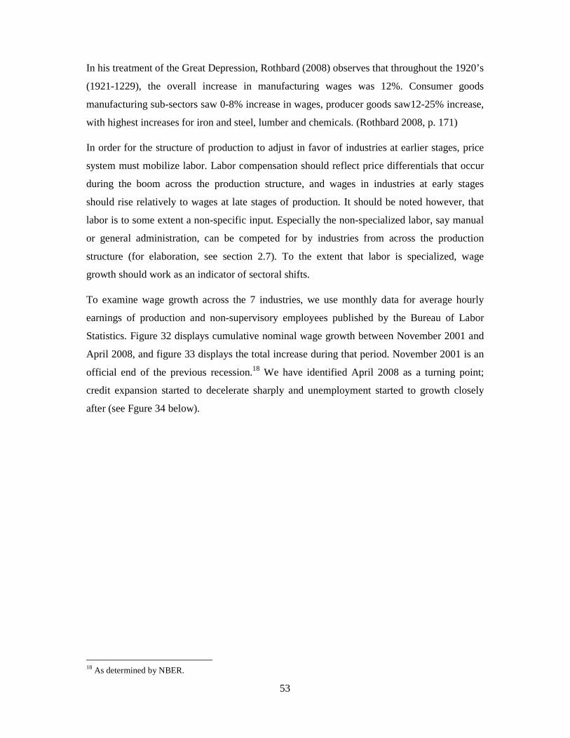
53

In his treatment of the Great Depression, Rothbard (2008) observes that throughout the 1920’s

(1921-1229), the overall increase in manufacturing wages was 12%. Consumer goods

manufacturing sub-sectors saw 0-8% increase in wages, producer goods saw12-25% increase,

with highest increases for iron and steel, lumber and chemicals. (Rothbard 2008, p. 171)

In order for the structure of production to adjust in favor of industries at earlier stages, price

system must mobilize labor. Labor compensation should reflect price differentials that occur

during the boom across the production structure, and wages in industries at early stages

should rise relatively to wages at late stages of production. It should be noted however, that

labor is to some extent a non-specific input. Especially the non-specialized labor, say manual

or general administration, can be competed for by industries from across the production

structure (for elaboration, see section 2.7). To the extent that labor is specialized, wage

growth should work as an indicator of sectoral shifts.

To examine wage growth across the 7 industries, we use monthly data for average hourly

earnings of production and non-supervisory employees published by the Bureau of Labor

Statistics. Figure 32 displays cumulative nominal wage growth between November 2001 and

April 2008, and figure 33 displays the total increase during that period. November 2001 is an

official end of the previous recession.18 We have identified April 2008 as a turning point;

credit expansion started to decelerate sharply and unemployment started to growth closely

after (see Fgure 34 below).

18 As determined by NBER.

54

FIGURE 32: CUMULATIVE WAGE GROWTH

Based on Bureau of Labor Statistics data

FIGURE 33: TOTAL WAGE GROWTH IN THE EXPANSION PERIOD

Retail Non-

durables

Utilities Construction

Durables

Wholesale

M&L

Wage

Growth

11.7% 15.1% 16.4% 18.3% 19.1% 19.5% 26.6%

When ordered from the lowest to the highest cumulative wage growth, we find one mismatch

compared to the expected order of wage growths. In particular, wage growth in wholesale

industry outpaced that of construction and slightly that of durable manufacturing. Other wage

growths are ordered as expected. We might also observe that wages grew slightly faster in

utilities than in non-durable manufacturing, a difference from the order we arrived at by

comparing regression coefficients for credit growth in the previous proposition. Also notable

is the very high wage growth in the mining & logging industry, which also corresponds to the

high regression coefficient of the credit growth variable for this industry. Timing of the sharp

wage increase in the mining & logging industry however coincides with the commodity boom

of 2006 and 2008 (see section 3.5.1. for details), and thus cannot be attributed solely to the

-5%

0%

5%

10%

15%

20%

25%

30%

No

v-0

1

Fe

b-0

2

Ma

y-0

2

Au

g-0

2

No

v-0

2

Fe

b-0

3

Ma

y-0

3

Au

g-0

3

No

v-0

3

Fe

b-0

4

Ma

y-0

4

Au

g-0

4

No

v-0

4

Fe

b-0

5

Ma

y-0

5

Au

g-0

5

No

v-0

5

Fe

b-0

6

Ma

y-0

6

Au

g-0

6

No

v-0

6

Fe

b-0

7

Ma

y-0

7

Au

g-0

7

No

v-0

7

Fe

b-0

8

Non-durables Mining & Logging Retail

Construction Durables Wholesale

Utilities

55

structure of production changes as described by the theory. The magnitude of cumulative

wage growth differentials, especially within the 15.1%-19.5% cluster, over more than 6 years

(figures 32 and 33) do not provide a strong message. Overall, wage growth data don’t

contradict the proposition 4, but fail to support it clearly.

3.4.3 PR OP OSI TI O N 5: JOB LOS S PA TTE R N

Proposition 5: At the end of upswing, unemployment should increase first and with greater

intensity in industries at early stages of production, and with some lag and lesser intensity in

industries at later stages.

When the boom ends and correction follows, we should see an asymmetric impact on labor

market across the stages of production. Although wage growth is a good indicator of

performance in the expansion period, its ability usefulness as a measure of sectoral patterns

becomes more doubtful in the contraction period due to downward wage rigidity. We thus

turn to lay-offs as an indicator of contraction severity across the structure of production.

Industries at early stages should suffer from bigger downturn and greater job losses as a

consequence. April 2008 marked the beginning of the credit growth deceleration. The first

sharp dip in credit growth was closely followed by the beginning of a sustained sharp growth

in unemployment, as seen in figure 34.

FIGURE 34: CREDIT EXPANSION AND UNEMPLOYMENT

We expect the ordering of the seven industries in line with propositions 3 and 4. Figure 35

displays cumulative sectoral job losses from April 2008, when credit growth sharply

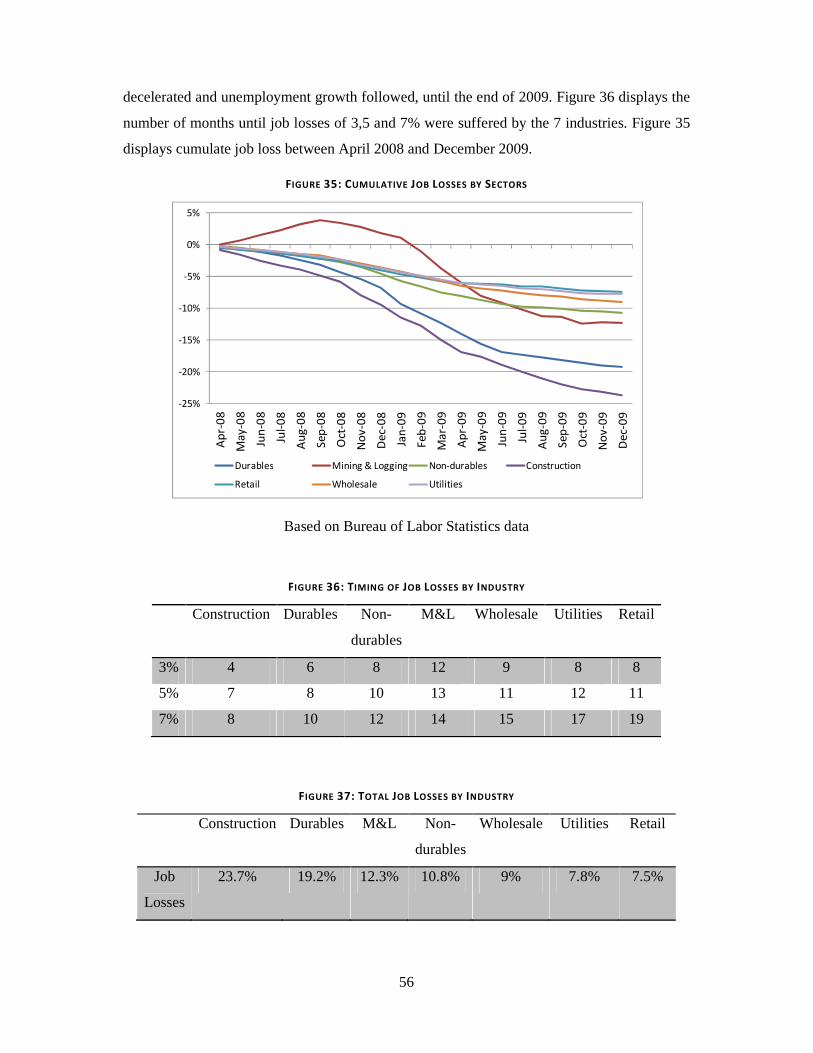
56

decelerated and unemployment growth followed, until the end of 2009. Figure 36 displays the

number of months until job losses of 3,5 and 7% were suffered by the 7 industries. Figure 35

displays cumulate job loss between April 2008 and December 2009.

FIGURE 35: CUMULATIVE JOB LOSSES BY SECTORS

Based on Bureau of Labor Statistics data

FIGURE 36: TIMING OF JOB LOSSES BY INDUSTRY

Construction Durables Non-

durables

M&L Wholesale Utilities Retail

3% 4 6 8 12 9 8 8

5% 7 8 10 13 11 12 11

7% 8 10 12 14 15 17 19

FIGURE 37: TOTAL JOB LOSSES BY INDUSTRY

Construction Durables M&L Non-

durables

Wholesale

Utilities Retail

Job

Losses

23.7% 19.2% 12.3% 10.8% 9% 7.8% 7.5%

-25%

-20%

-15%

-10%

-5%

0%

5%A

pr-

08

Ma

y-0

8

Jun

-08

Jul-

08

Au

g-0

8

Se

p-0

8

Oct

-08

No

v-0

8

De

c-0

8

Jan

-09

Fe

b-0

9

Ma

r-0

9

Ap

r-0

9

Ma

y-0

9

Jun

-09

Jul-

09

Au

g-0

9

Se

p-0

9

Oct

-09

No

v-0

9

De

c-0

9

Durables Mining & Logging Non-durables Construction

Retail Wholesale Utilities

57

The results show that timing and extent of the job losses displays some deviations from what

the expectations based on the theory are. The three industries of earlier stages of production

did lose the most jobs; 23.7% for construction, 19.2% for durable manufacturing and 12.3%

for mining. Their order, both in terms of timing and total losses, is however slightly different.

In particular, the mining & logging industry kept hiring until early 2009, while all the other

sectors were shedding jobs. This phenomenon is attributable to high commodity prices

(section 3.5.1), with crude oil peaking in July 2008 and remaining fairly high until October

2008. After hiring in the mining & logging industry peaked, extent of job losses was large.

Construction and durable manufacturing were fastest to lose jobs, retail and utilities were the

slowest. Construction and durables lost the most jobs, retail and utilities lost the least. Thus,

with an exception of mining & logging attributable to the commodity boom, the expected

pattern emerged and proposition 5 is supported.

3.5. RELATIVE PRICES

In the following sections, we will closely examine the development of relative prices

throughout the business cycle. A phenomenon specific to the period that will be clearly visible

in all the time series for prices at early stages of production analyzed below, was the

commodity boom of 2006-2008. A brief summary of the commodity boom will provide

context and enable better understanding for the propositions 6, 7 and 8 in the section on

relative prices.

3.5.1 CO MM ODITY BO OM OF 2006-2008

Commodity prices were increasing from the beginning of the examined period, however

prices began to increase more sharply in the middle of 2006, after a brief downturn.

Commodity boom peaked in April 2008 for metals and minerals, in June for agricultural

commodities and in July for crude oil. Crude oil peaked at $93/barrel, marking a 94% annual

price increase. Crude oil prices saw the most exuberant development towards the end of the

boom. Agricultural commodities displayed considerably lower price variability than crude oil

and metals.

58

FIGURE 38: COMMODITY CLASSES

Based on World Bank data

Baffes and Haniotis (2010) analyzed development and causes of the commodity boom,

identifying several influences. US dollar, being the key currency in commodity transactions,

was depreciating throughout the observed period, which strengthened the demand from the

non-dollar countries. Another reason, particularly with respect to supply side of non-

agricultural commodities, was the low previous investments into extractive activities. As we

saw above in the section on industrial activity, spiking commodity prices gave a strong boost

to the mining industry, which lasted even after activity began to decline in other sectors.

There are several factors that lead to increase in agricultural commodity prices. First, there

were some unfavorable climate conditions. Firstly, there were three droughts in Australia

between 2002 and 2008. Secondly, worldwide policies of promoting bio fuels diverted some

of the agricultural commodities into energy use, which constitutes a minor demand shock. The

third most quoted explanation is the rising demand from the developing world. There is no

clear agreement over the relative importance of these factors.

Expansionary monetary policies throughout the observed period also supported heavier

investment demand for all commodities. The general trend of bundling commodity into

trading indexes and including them in portfolios is sometimes referred to as financialization of

commodities. Implications of this phenomenon have been examined by Tang and Xiong

(2010) with the following conclusion:

0

100

200

300

400

500

600

700

Oct

-01

Feb

-02

Jun

-02

Oct

-02

Feb

-03

Jun

-03

Oct

-03

Feb

-04

Jun

-04

Oct

-04

Feb

-05

Jun

-05

Oct

-05

Feb

-06

Jun

-06

Oct

-06

Feb

-07

Jun

-07

Oct

-07

Feb

-08

Jun

-08

Oct

-08

Feb

-09

Jun

-09

Oct

-09

Agricultural Commodities Metals & Minerals Crude Oil

59

“As a result of the financialization process, the price of an individual commodity is no longer

simply determined by its supply and demand. Instead, prices are also determined by the

aggregate risk appetite for financial assets and investment behavior of diversified commodity

index investors.” (p. 30)

Thus, the commodity market becomes less segmented and a price increase of one commodity

class can lead to price increases of all commodities to the extent they are correlated and

bundled together in commodity indexes. The crude oil price rally of 2008 could thus have

some impact on the general rise of commodity prices. Two most often quoted commodity

indices are the S&P Goldman Sachs Commodity Index, separately quoted since mid 2006,

and the Dow Jones AIG quoted since late 2007. Figure 39 graphs S&P GSCI Index from the

beginning of its inception. When the commodities peaked after less than two years of its

existence, the index was up 47% since its first quote.

FIGURE 39: S&P GOLDMAN SACHS COMMODITY INDEX

Based on Bloomberg data

Baffes and Haniotis (2010) also identify three major reasons for why investment fund

managers having increasingly turned to commodities. First, existing assets were becoming

increasingly correlated and commodities presented a new diversification opportunity. Second,

diversification away from dollar-denominated financial assets into physical assets. The third

reason is the impact of excess liquidity caused by lax monetary policy on the increasing

inclusion of commodities into investment portfolios.

0

20

40

60

80

100

120

140

160

Jul-

06

No

v-0

6

Ma

r-0

7

Jul-

07

No

v-0

7

Ma

r-0

8

Jul-

08

No

v-0

8

Ma

r-0

9

Jul-

09

No

v-0

9

S&P GSCI

60

The last reason in particular is in line with the ABCT. The theory predicts that a policy

induced credit expansion would fuel investments at early stages of production. Particularly

those commodities that are processed heavily before their further use should increase in price.

Disaggregation of aggregate commodity price statistics and determination of how much

processing particular commodities are subject to would be required to make a more

conclusive quantitative analysis. However, the fact that metals and crude oil have seen a

significantly sharper price increase than agricultural commodities (figure xx) is in line with

the theory, as metals and minerals require a much longer sequence of technological

processing than agricultural commodities do. Intuition suggests that the process of turning a

mountain side deposit of iron ore into an electric shaver is more intricate and time demanding

than turning a plot of arable land into popcorn. If we substitute raw iron for the iron ore

deposit and corn for the arable land, intuition still holds. Thus, metals and minerals can be

considered earlier stages than agricultural commodities.

End of the commodity boom closely follows a first major deceleration in credit growth rate

that took place in April 2008 (figure 40).

FIGURE 40: CREDIT EXPANSION AND COMMODITY PRICES

Based on FRED and Bloomberg data

The last sharp temporary spike upwards before credit growth began its decrease to negative

values corresponds to Federal Reserve’s fund rate reduction from 2% to 1% in October 2008

and introduction of a number of emergency lending facilities described above (section 3.2.4).

61

When source fueling the malinvestment and distorted relative prices started to dry up, a sharp

correction followed.

3.5.2 PR OP OS I TI O N 6: CONS UME R AND PR OD UC E R PRIC E S D URI NG THE CRE DI T

EXPA NSI O N

Proposition 6: The ratio of producer prices to consumer prices tends to rise after the

initiation of a credit expansion.

A sharp increase in the rate of credit growth began during the second quarter of 2002. The

annual growth rate exceeded 5% in September of 2002 and remained above that rate until

August 2008. September 2008 marks a beginning of sharp deceleration in credit growth,

although credit did not contract until September 2009. Figure 41 plots the annual percentage

growth of credit and the annual percentage growth of the ratio of aggregate producer price

index to the consumer price index (PPI/CPI).

FIGURE 41: CREDIT AND PPI/CPI RATIO

Based on FRED data

The credit growth rate made a sharp upward swing from 4 to 7% in August and October 2002,

then retained high levels until April 2008. We can see that PPI/CPI starts growing in October

2002, shortly after the rate of credit growth picks up. The PPI/CPI ratio then grows

throughout the period with a brief exception in the 4th quarter of 2006, it starts to decelerate in

August 2008, shortly after the sharp credit growth deceleration begins. In November 2008, it

began to fall sharply. Relative price development of consumer prices and producer prices

during the credit expansion thus support the proposition 6.

-20%

-15%

-10%

-5%

0%

5%

10%

15%

No

v-0

1

Ma

r-0

2

Jul-

02

No

v-0

2

Ma

r-0

3

Jul-

03

No

v-0

3

Ma

r-0

4

Jul-

04

No

v-0

4

Ma

r-0

5

Jul-

05

No

v-0

5

Ma

r-0

6

Jul-

06

No

v-0

6

Ma

r-0

7

Jul-

07

No

v-0

7

Ma

r-0

8

Jul-

08

No

v-0

8

Ma

r-0

9

Jul-

09

No

v-0

9

dCredit, annual d(PPI/CPI), annual

62

Propositions 7 and 8 will elaborate in more detail on proposition 6. Proposition 7 will be more

focused on the upswing phase of the cycle, while proposition 8 will add the bust-related

correction of relative prices into analysis.

3.5.3. PROPO SITIO N 7: PRIC E S AL ONG T HE ST RUCT URE OF PR ODUC TI O N

Proposition 7: During the expansion phase, prices of producer goods closest to final

consumption tend to decline relative to the prices of producer goods further away from the

later stages of production.

This proposition follows the widening of price differentials across the structure of production.

With the onset of credit expansion, price differentials between products at different stages

arise. The earlier the stage, the greater the magnitude of the price increase should be. When

prices of products at different stages are plotted over time, they should form layers starting

with the earliest stages and ending with the latest stages. At the end of credit expansion, the

price differentials should narrow with the correction being sharper for earlier sages than for

the late stages. We will focus on the reversal in more detail in next proposition.

Apart from the discount effect driving price differentials along the structure of production and

driving investments particularly at the early stages of production, the theory also asserts some

price increases of consumer goods early in the boom. This reflects the both consequences of

credit expansion: malinvestments and over-consumption (see Figure 8). The overconsumption

should take place early in the economy’s business cycle trajectory. After it runs its course,

overinvestment is the dominant phenomenon of the boom (see Figure 9) The

overconsumption phenomenon is less suitable for being formulated into a clear proposition as

it doesn’t imply any particular development. Overconsumption can mean an increase in

consumption that could in short-run be reflected in CPI growth acceleration. On the other

hand, it can mean continuation of the previous levels of consumption in the situation when

equilibrium in the market for loanable funds would require a decrease in consumption.

Nevertheless, we shall also include consumer prices into our analysis and comment on their

development with regard to the overconsumption phenomenon.

Producer price indices (PPI) and the consumer price index (CPI) are the most suitable data to

test this proposition. Available data for the aggregate production enable us to examine price

changes for four stages of production. From the earliest to the latest stage, Figure 42 includes

PPI for crude materials for further processing, PPI for intermediate materials, PPI for finished

goods and the consumer price index (CPI). Price differentials were growing throughout the

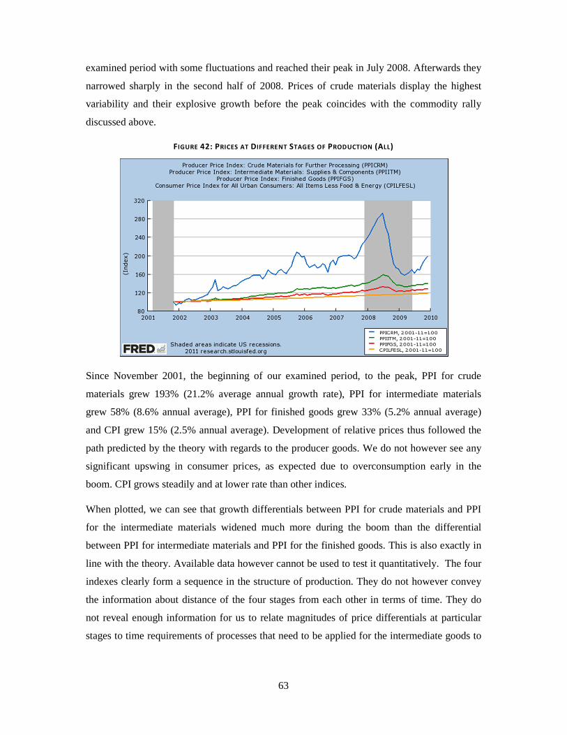
63

examined period with some fluctuations and reached their peak in July 2008. Afterwards they

narrowed sharply in the second half of 2008. Prices of crude materials display the highest

variability and their explosive growth before the peak coincides with the commodity rally

discussed above.

FIGURE 42: PRICES AT DIFFERENT STAGES OF PRODUCTION (ALL)

Since November 2001, the beginning of our examined period, to the peak, PPI for crude

materials grew 193% (21.2% average annual growth rate), PPI for intermediate materials

grew 58% (8.6% annual average), PPI for finished goods grew 33% (5.2% annual average)

and CPI grew 15% (2.5% annual average). Development of relative prices thus followed the

path predicted by the theory with regards to the producer goods. We do not however see any

significant upswing in consumer prices, as expected due to overconsumption early in the

boom. CPI grows steadily and at lower rate than other indices.

When plotted, we can see that growth differentials between PPI for crude materials and PPI

for the intermediate materials widened much more during the boom than the differential

between PPI for intermediate materials and PPI for the finished goods. This is also exactly in

line with the theory. Available data however cannot be used to test it quantitatively. The four

indexes clearly form a sequence in the structure of production. They do not however convey

the information about distance of the four stages from each other in terms of time. They do

not reveal enough information for us to relate magnitudes of price differentials at particular

stages to time requirements of processes that need to be applied for the intermediate goods to

64

pass another stage down the structure of production. Such quantification is concealed in the

statistical aggregates.

Data availability enables exploration of the relative prices across the structure of production

for two particular industries: food and energy. In both cases, the commodity market rally of

2008 had a much greater impact than it had on the total production. Also more visible is a

brief commodity market correction in mid 2006. In case of energy, the differential between

PPI for the crude materials and intermediate goods widens much more than the differential

between PPI for the intermediate goods and PPI for the finished goods.

FIGURE 43: PRICES AT DIFFERENT STAGES OF PRODUCTION (ENERGY INDUSTRY)

The former widens more significantly towards the peak. All three indices peaked in August

2008. Since the beginning of observed period to the peak in July 2008, PPI for the crude

energy materials rose by 372% (average annual growth of 32%), PPI for the intermediate

energy goods grew by 156% (18.3% annually) and PPI for the finished energy goods by

136% (16.7% annually). CPI for energy is not included in the graph, as at the given scale, it

would visually merge with PPI for the finished energy goods. It grew 132% (16.3% annually).

As in the case of economy-wide price indices, CPI did not display any upward swing

attributable to the overconsumption phenomenon. The exceptionally high increase of the

crude materials PPI is largely accounted for by the crude oil price development. As with the

economy-wide prices, the energy industry also display widening of the price differentials

implied by the theory.

65

Prices at different stages of production in the food industry (Figure 44) display one deviation

from difference. The price differentials between products of the earliest stage and the other

stages first widened and then narrowed and essentially disappeared in mid 2006 commodity

price correction. As seen in the Figure 44, this corresponds to a sharp dip of the crude

foodstuff and feedstuff PPI at the end of 2005 and beginning of 2006, only to rebound swiftly

and grow further. This development follows a short-lived but sharp dip of nitrogen fertilizer

prices at the time. After that the price differentials resumed their previous development, one

that the theory predicts. They widen considerably and narrow sharply at boom’s end.19

FIGURE 44: PRICES AT DIFFERENT STAGES OF PRODUCTION (FOOD INDUSTRY)

Since the beginning of the examined period to the peak of July 2008, PPI for the crude

foodstuff was up 75% (10.5% average annual growth), PPI for intermediate foods was up

66% (9.5% annually), PPI for finished foods was up 28% (4.6% annually) and CPI for food

op 23% (3.8% annually). Apart from the sharp decline of the PPI for crude foodstuff

attributable to a decrease of nitrogen fertilizer prices, producer prices development follows the

path suggested by the theory.

Having examined development of relative prices for the economy as a whole and for two

particular industries, we find support for the proposition 7. On the other hand, we found no

clear evidence suggesting overconsumption.

19 See appendix for a nitrogen fertilizer price chart

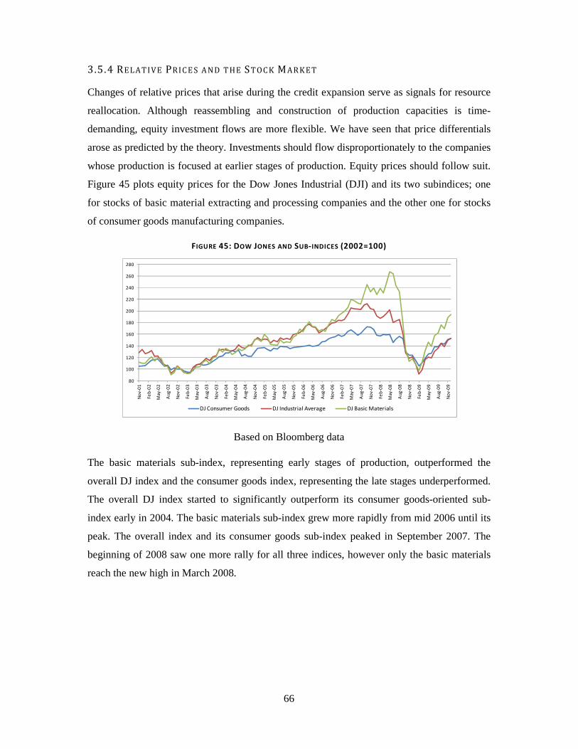
66

3.5.4 RE L ATIVE PRIC E S A ND T HE S TOC K MARK E T

Changes of relative prices that arise during the credit expansion serve as signals for resource

reallocation. Although reassembling and construction of production capacities is time-

demanding, equity investment flows are more flexible. We have seen that price differentials

arose as predicted by the theory. Investments should flow disproportionately to the companies

whose production is focused at earlier stages of production. Equity prices should follow suit.

Figure 45 plots equity prices for the Dow Jones Industrial (DJI) and its two subindices; one

for stocks of basic material extracting and processing companies and the other one for stocks

of consumer goods manufacturing companies.

FIGURE 45: DOW JONES AND SUB-INDICES (2002=100)

Based on Bloomberg data

The basic materials sub-index, representing early stages of production, outperformed the

overall DJ index and the consumer goods index, representing the late stages underperformed.

The overall DJ index started to significantly outperform its consumer goods-oriented sub-

index early in 2004. The basic materials sub-index grew more rapidly from mid 2006 until its

peak. The overall index and its consumer goods sub-index peaked in September 2007. The

beginning of 2008 saw one more rally for all three indices, however only the basic materials

reach the new high in March 2008.

80

100

120

140

160

180

200

220

240

260

280

No

v-0

1

Feb

-02

May

-02

Au

g-0

2

No

v-0

2

Feb

-03

May

-03

Au

g-0

3

No

v-0

3

Feb

-04

May

-04

Au

g-0

4

No

v-0

4

Feb

-05

May

-05

Au

g-0

5

No

v-0

5

Feb

-06

May

-06

Au

g-0

6

No

v-0

6

Feb

-07

May

-07

Au

g-0

7

No

v-0

7

Feb

-08

May

-08

Au

g-0

8

No

v-0

8

Feb

-09

May

-09

Au

g-0

9

No

v-0

9

DJ Consumer Goods DJ Industrial Average DJ Basic Materials

67

3.5.5 PR OP OS I TI O N 8: COR RE C TI ON OF THE D IST ORTE D RE L ATIV E PRIC E S

Proposition 8: The prices of consumer goods rise relative to the prices of producer goods,

reversing the initial shift in relative prices as credit is contracted towards the end of the cycle.

Similarly, prices of producer goods at later stages will rise relative to prices of producer

goods at earlier stages.

Le Roux (1999) follows his version of the proposition into its implications and notes that “the

relative prices of consumer goods to the producer goods will show an increase and the

evaluated prices will, if translated into a graph, assume a parabolic shape.”(p. 27) The same

pattern can be expected with regard to prices of producer goods situated closer to consumer

goods in the structure of production relative to prices of producer goods situated further away

from consumer goods in the structure of production. The theory thus predicts a particular

development of prices along the structure of production. The credit expansion should lead to

widening of price differentials between prices of products at the earlier stages and the later

stages during the expansion and then to narrowing of those stages when the credit expansion

ceases. Differentials between two relatively earlier subsequent stages should widen to greater

extent than margins of two relatively later stages.

To examine whether that was the case, we can use producer price indices for various stages

and consumer price index as a measure of price of products at the latest stage. We take the

price indices from the proposition 7 measuring development of prices from the base of 100 at

the beginning of the observed period and devise ratios of two stages next to each other, first

for the whole economy and then for two particular industries; energy and food. Again, the

choice of industries was to large extent guided by data availability.

The ratios should start rising and remain elevated while the credit expansion lasts. When the

credit growth decelerates, the ratios should start declining. When graphed, the ratios should

resemble a negative-coefficient parabola. Moreover, the magnitude of increase and then

decrease for the ratio of two prices at stages further away from consumption should be greater

than that of two stages closer to consumption. For each ratio graphed over time, we can add a

best fit polynomial in order to determine whether the ratio can be said to have followed a

parabolic trajectory, and if so how good the fit is. The higher the degree of a polynomial, the

more closely it will follow the actual graph. In order for the polynomial to remain some clear

shape while allowing it for a reasonably good fit, we shall use a degree 4 polynomial.

68

The development of the ratio between crude materials PPI and intermediate materials PPI for

the overall economy during the observed period is well represented with a parabolic shape

(Figure 46).

FIGURE 46: PRICE DIFFERENTIALS 1 (ALL)

The price differential is fairly high, with the ratio peaking in May 2008, when the price

increase for the crude materials PPI was a 1.86 multiple of the price increase for the

intermediate materials PPI. The multiple then sharply corrected to as low as 1.19 in March

2009, erasing most of the price differential between products of the two stages.

Price differential between the intermediate PPI and the finished goods PPI is also well

represented with a parabolic shape (Figure 47).

y = -9E-14x4 + 1E-08x3 - 0.0008x2 + 20.364x - 196180

R² = 0.6522

0.9

1.1

1.3

1.5

1.7

1.9

No

v-0

1

Mar

-02

Jul-

02

No

v-0

2

Mar

-03

Jul-

03

No

v-0

3

Mar

-04

Jul-

04

No

v-0

4

Mar

-05

Jul-

05

No

v-0

5

Mar

-06

Jul-

06

No

v-0

6

Mar

-07

Jul-

07

No

v-0

7

Mar

-08

Jul-

08

No

v-0

8

Mar

-09

Jul-

09

No

v-0

9

PPI: Crude / Intermediate

PPI: Crude / Intermediate Best Fit Degree 4 Polynomial

69

FIGURE 47: PRICE DIFFERENTIALS 2 (ALL)

The price differential between products of these two stages was much lower than between the

previous two stages. The ratio peaked at 1.19 in July 2008 and corrected to as low as 1.07 by

June 2009.

Ratio between the finished goods PPI and CPI followed a very similar parabolic shape as the

ratio between the previous two stages, only fluctuating in a slightly narrower band.

FIGURE 48: PRICE DIFFERENTIALS 3 (ALL)

It peaked at 1.16 in July 2008 and corrected to 1.05 by March 2009.

y = -8E-15x4 + 1E-09x3 - 7E-05x2 + 1.659x - 15614

R² = 0.8965

0.98

1.03

1.08

1.13

1.18

No

v-0

1

Mar

-02

Jul-

02

No

v-0

2

Mar

-03

Jul-

03

No

v-0

3

Mar

-04

Jul-

04

No

v-0

4

Mar

-05

Jul-

05

No

v-0

5

Mar

-06

Jul-

06

No

v-0

6

Mar

-07

Jul-

07

No

v-0

7

Mar

-08

Jul-

08

No

v-0

8

Mar

-09

Jul-

09

No

v-0

9

PPI: Intermediate / Finished

PPI: Intermediate / Finished Best Fit Degree 4 Polynomial

y = -7E-15x4 + 1E-09x3 - 6E-05x2 + 1.4558x - 13842

R² = 0.8159

0.98

1.02

1.06

1.1

1.14

No

v-0

1

Mar

-02

Jul-

02

No

v-0

2

Mar

-03

Jul-

03

No

v-0

3

Mar

-04

Jul-

04

No

v-0

4

Mar

-05

Jul-

05

No

v-0

5

Mar

-06

Jul-

06

No

v-0

6

Mar

-07

Jul-

07

No

v-0

7

Mar

-08

Jul-

08

No

v-0

8

Mar

-09

Jul-

09

No

v-0

9PPI: Finished / CPI

PPI Finished / CPI Best Fit Degree 4 Polynomial

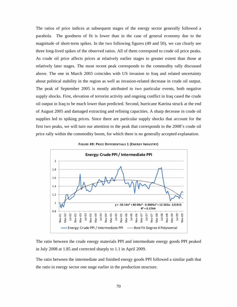
70

The ratios of price indices at subsequent stages of the energy sector generally followed a

parabola. The goodness of fit is lower than in the case of general economy due to the

magnitude of short-term spikes. In the two following figures (49 and 50), we can clearly see

three long-lived spikes of the observed ratios. All of them correspond to crude oil price peaks.

As crude oil price affects prices at relatively earlier stages to greater extent than those at

relatively later stages. The most recent peak corresponds to the commodity rally discussed

above. The one in March 2003 coincides with US invasion to Iraq and related uncertainty

about political stability in the region as well as invasion-related decrease in crude oil output.

The peak of September 2005 is mostly attributed to two particular events, both negative

supply shocks. First, elevation of terrorist activity and ongoing conflict in Iraq cased the crude

oil output in Iraq to be much lower than predicted. Second, hurricane Katrina struck at the end

of August 2005 and damaged extracting and refining capacities. A sharp decrease in crude oil

supplies led to spiking prices. Since there are particular supply shocks that account for the

first two peaks, we will turn our attention to the peak that corresponds to the 2008’s crude oil

price rally within the commodity boom, for which there is no generally accepted explanation.

FIGURE 49: PRICE DIFFERENTIALS 1 (ENERGY INDUSTRY)

The ratio between the crude energy materials PPI and intermediate energy goods PPI peaked

in July 2008 at 1.85 and corrected sharply to 1.1 in April 2009.

The ratio between the intermediate and finished energy goods PPI followed a similar path that

the ratio in energy sector one stage earlier in the production structure.

y = -5E-14x4 + 8E-09x3 - 0.0005x2 + 12.563x - 121915

R² = 0.57640.8

1

1.2

1.4

1.6

1.8

2

No

v-0

1

Mar

-02

Jul-

02

No

v-0

2

Mar

-03

Jul-

03

No

v-0

3

Mar

-04

Jul-

04

No

v-0

4

Mar

-05

Jul-

05

No

v-0

5

Mar

-06

Jul-

06

No

v-0

6

Mar

-07

Jul-

07

No

v-0

7

Mar

-08

Jul-

08

No

v-0

8

Mar

-09

Jul-

09

No

v-0

9

Energy: Crude PPI / Intermediate PPI

Energy: Crude PPI / Intermediate PPI Best Fit Degree 4 Polynomial

71

FIGURE 50: PRICE DIFFERENTIALS 2 (ENERGY INDUSTRY)

The three peaks explained above are also distinctly visible. The price differentials were

however much smaller and kept the ratio in a narrow band. The ratio peaked at 1.08 in July

2008 and corrected to 0.98 in June 2009, not only completely erasing the price differential

between the two stages but also turning it negative.

The ratio between the crude foodstuff PPI and the intermediate foodstuff PPI peaked in

January 2008 at 1.12 and fell to 0.91 in July 2009.

FIGURE 51: PRICE DIFFERENTIALS 1 (FOOD INDUSTRY)

y = -8E-15x4 + 1E-09x3 - 7E-05x2 + 1.7272x - 16498

R² = 0.3557

0.96

1

1.04

1.08

No

v-0

1

Mar

-02

Jul-

02

No

v-0

2

Mar

-03

Jul-

03

No

v-0

3

Mar

-04

Jul-

04

No

v-0

4

Mar

-05

Jul-

05

No

v-0

5

Mar

-06

Jul-

06

No

v-0

6

Mar

-07

Jul-

07

No

v-0

7

Mar

-08

Jul-

08

No

v-0

8

Mar

-09

Jul-

09

No

v-0

9

Energy: Intermediate PPI / Finished PPI

Energy: Intermediate PPI / Finished PPI Best Fit Degree 4 Polynomial

y = -2E-14x4 + 4E-09x3 - 0.0002x2 + 5.3892x - 51727

R² = 0.50840.85

0.9

0.95

1

1.05

1.1

1.15

No

v-0

1

Ma

r-0

2

Jul-

02

No

v-0

2

Ma

r-0

3

Jul-

03

No

v-0

3

Ma

r-0

4

Jul-

04

No

v-0

4

Ma

r-0

5

Jul-

05

No

v-0

5

Ma

r-0

6

Jul-

06

No

v-0

6

Ma

r-0

7

Jul-

07

No

v-0

7

Ma

r-0

8

Jul-

08

No

v-0

8

Ma

r-0

9

Jul-

09

No

v-0

9

Food: Crude PPI / Intermediate PPI

Food: Crude PPI / Intermediate PPI Best Fit Degree 4 Polynomial

72

The parabola makes for a fairly good fit of the ratio’s development. The ratio’s most notable

departure from the parabolic shape was during the temporary sharp decrease of the crude

foodstuff PPI, then quickly rebounded. As discussed in proposition 7, the brief dip and

rebound of the crude foodstuff PPI can be partially attributable to similar development of

nitrogen fertilizer prices.

Ratio between the intermediate foodstuff PPI and the finished goods PPI peaked at 1.29 in

July 2008, then fell to 1.14 April 2009.

FIGURE 52: PRICE DIFFERENTIALS 2 (FOOD INDUSTRY)

Unlike in other observed ratios, the one in point departs significantly from a parabolic shape.

The price differential that arose throughout the boom remained fairly high even after

differentials between other stages we have examine narrowed greatly or even disappeared.

The development of the ratio between finished foods PPI and CPI assumes a parabolic shape,

even though its confinement in a narrow band means that even mild short-term fluctuations

can easily distort the shape It peaked at 1.05 in June 2008, then fell to 0.99 March in 2009.

y = -8E-14x4 + 1E-08x3 - 0.0007x2 + 19.005x - 183588

R² = 0.76310.93

0.98

1.03

1.08

1.13

1.18

1.23

1.28

No

v-0

1

Ma

r-0

2

Jul-

02

No

v-0

2

Ma

r-0

3

Jul-

03

No

v-0

3

Ma

r-0

4

Jul-

04

No

v-0

4

Ma

r-0

5

Jul-

05

No

v-0

5

Ma

r-0

6

Jul-

06

No

v-0

6

Ma

r-0

7

Jul-

07

No

v-0

7

Ma

r-0

8

Jul-

08

No

v-0

8

Ma

r-0

9

Jul-

09

No

v-0

9

Food: Intermediate PPI / Finished PPI

Food: Intermediate PPI / Finished PPI Best Fit Degree 4 Polynomial

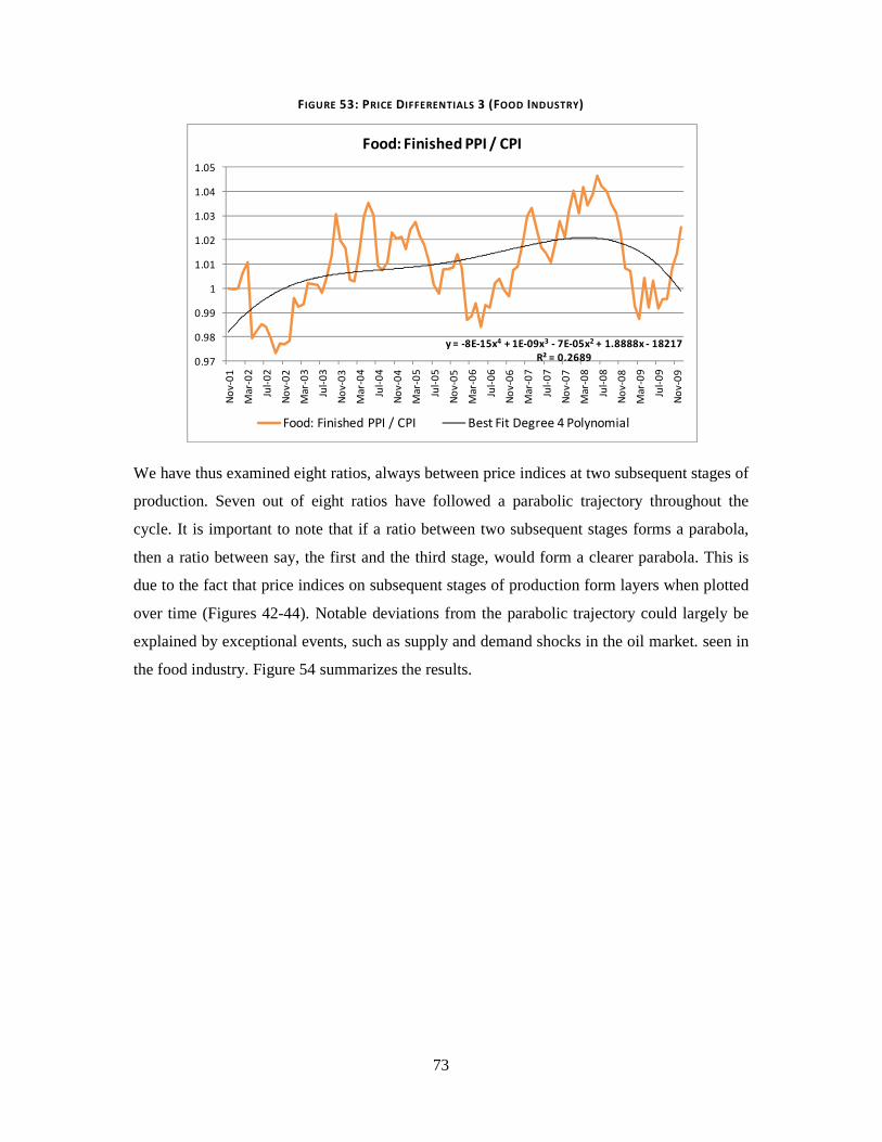
73

FIGURE 53: PRICE DIFFERENTIALS 3 (FOOD INDUSTRY)

We have thus examined eight ratios, always between price indices at two subsequent stages of

production. Seven out of eight ratios have followed a parabolic trajectory throughout the

cycle. It is important to note that if a ratio between two subsequent stages forms a parabola,

then a ratio between say, the first and the third stage, would form a clearer parabola. This is

due to the fact that price indices on subsequent stages of production form layers when plotted

over time (Figures 42-44). Notable deviations from the parabolic trajectory could largely be

explained by exceptional events, such as supply and demand shocks in the oil market. seen in

the food industry. Figure 54 summarizes the results.

y = -8E-15x4 + 1E-09x3 - 7E-05x2 + 1.8888x - 18217

R² = 0.26890.97

0.98

0.99

1

1.01

1.02

1.03

1.04

1.05

No

v-0

1

Mar

-02

Jul-

02

No

v-0

2

Mar

-03

Jul-

03

No

v-0

3

Mar

-04

Jul-

04

No

v-0

4

Mar

-05

Jul-

05

No

v-0

5

Mar

-06

Jul-

06

No

v-0

6

Mar

-07

Jul-

07

No

v-0

7

Mar

-08

Jul-

08

No

v-0

8

Mar

-09

Jul-

09

No

v-0

9

Food: Finished PPI / CPI

Food: Finished PPI / CPI Best Fit Degree 4 Polynomial

74

FIGURE 54: PRICE DIFFERENTIALS (SUMMARY)

RATIO Peak

Differential

Time of

Peak

Bottom

Differential

Time of

Bottom

Parabola R2

Crude/Intermediate

(US Economy)

86% May-08 19% Mar-09 Yes 65%

Intermediate/Finished

(US Economy)

19% Jul-08 7% Jun-09 Yes 90%

Finished/CPI

(US Economy)

16% Jul-08 5% Mar-09 Yes 82%

Crude/Intermediate

(Energy)

85% Jul-08 10% Apr-09 Yes 58%

Intermediate/Finished

(Energy)

8% Jul-08 -2% Jun-09 Yes 36%

Crude/Intermediate

(Food)

12% Jan-08 -9% Jul-09 Yes 51%

Intermediate/Finished

(Food)

29% Jul-08 14% Apr-09 No -

Finished/CPI

(Food)

5% Jun-08 -1% Mar-09 Yes 27%

Peaks of the ratios and their post-correction bottoms coincide for most ratios, suggesting an

economy wide phenomena, rather than sector-specific changes in relative prices. Moreover,

the price differentials between two relatively earlier stages were greater at the peak as

between two relatively later stages, also in line with the theory. With the exception of one

ratio in the food industry, the rations peaked within a one quarter after the first significant

downswing in credit growth. The expected development of relative prices was best seen in the

data for the overall economy. Most ambiguity and less precise fit of parabola, as well as the

only-one non-parabolic shape, was seen in the food industry. Overall, parabolic shape of

examined ratios supports the proposition 8.

75

4. CONCLUSION

As a part of the present paper, we provided a comprehensive exposition of the Austrian

business cycle theory and a brief description of the US economy in the period of 2001-2009.

The key aim of the paper was to apply the Austrian business cycle theory to the economic

cycle of 2001-2009 in the United States economy, when a period of vigorous economic

expansion was followed by a sharp downturn of 2007-2009. In order to determine to what

extent the theory provides a consistent explanation of the observed economic phenomena, we

confronted 8 propositions implied by the theory with economic data. The research was

structured into 3 major areas.

The first research area was focused on credit expansion and the market for loanable funds. In

line with the theory, we established that a disequilibrium in the market for loanable funds

appeared shortly after a monetary shock in the form of significant acceleration in the bank

credit growth. The disequilibrium was represented with a gap between investment and saving

and lasted throughout most of the expansion phase. The phenomenon was reverted after a

sharp deceleration of bank credit growth at the beginning of the economic downturn. We

tested for independence of credit growth and increases in savings, a condition needed for the

described situation to occur, with positive results. Development of slope of the yield curve

throughout the recession also corresponded to presence of a monetary shock in the form of a

bank credit expansion unsupported by increased savings. We thus identified presence of

conditions that the Austrian business cycle theory regards as cycle-generating.

The second research area was focused on sectoral patterns and the labor market. We matched

7 industries with stages along the structure of production as represented by the Hayekian

triangle. In order to determine impact of credit expansion on performance of the 7 industries

throughout the cycle, we used a simple regression model to link growth of sector-specific

employment to credit growth. The results were supportive of the theory as credit expansion

had a greater influence on industries matched with early stages of production. Wage growth

throughout the expansion period displayed more ambiguous results. Although the wage

largely corresponded to the theory, differentials across the sectors were not large and the

wholesale industry emerged as an exception. Its growth during the expansion phase exceeded

those of construction and durable manufacturing, both industries with higher expected growth

based on the theory. Data on depth and timing of job losses across the structure of production

76

in the contraction period approximately followed patterns predicted by the theory, but saw

some deviations. Development in the mining and logging industry can be seen as the most

significant departure from the theory. Timing and depth of job losses in mining and logging

corresponded to industries at approximately middle stages of the structure of production,

while the industry is positioned at the earliest stage in our sample. Sharp and quick downturn

in construction is in line with the theory as well. Nevertheless, the exceptional intensity of the

contraction and the extent of job losses in contraction in the 2007-2009 recession requires an

explanation beyond a general business cycle theory.

Third and the last research area of the paper focused on the structure of relative prices.

Relative prices drive resource allocation, and the theory predicts their specific development in

the course of the business cycle. In line with the theory, producer prices increased relative to

consumer prices following the onset of credit expansion and decreased following the

contraction. In order to disaggregate the price level, we used data specific to individual stages

of production of the US economy in general, and of the energy and food industry in particular.

Such methodology enabled a detailed scrutiny of relative price structure development. Data

was in line with the theory as price differentials between the stages of production opened in

favor of the early stages in the boom phase, then narrowed or closed in the contraction phase.

Significant deviations from the expected trajectory could be largely explained by exceptional

events, such as oil supply shocks. No clear evidence in support of the overconsumption

phenomenon postulated by the theory was found.

Overall, we conclude that the business cycle of 2001-2009 ended with the recession of 2007-

2009 in the US economy can to large extent be explained by the Austrian business cycle

theory. The theory’s weakness was seen in its less satisfactorily ability to account for the

labor market dynamics during the business cycle. On the other hand, the theory exhibits its

main strengths in accounting for development of relative prices and linking them to conditions

in the market for loanable funds.

77

REFERENCES

BAFFES, J., HANIOTIS. T.: Placing the 2006/08 Commodity Price Boom into Perspective,

Policy Research Working Paper #5371, The World Bank Development Prospects Group, 2010

BARNETT, W., BLOCK, W.: Professor Tullock on Austrian Business Cycle Theory, The

Dynamics of Intervention: Regulation and Redistribution in the Mixed Economy, Advances in

Austrian Economics, Volume 8, 2005, p. 431-443

BLOCK, W.: Yes, We Have No Chaff: A Reply to Wagner’s “Austrian Cycle Theory: Saving

the Wheat While Discarding the Chaff”, The Quarterly Journal of Austrian Economics, Vol. 4,

No. 1, Spring 2001, p. 63-73

CALLAHAN, G., GARRISON, R.W.: Does the Austrian Business Cycle Theory Help

Explain the Dot-Com Boom and Bust?, The Quarterly Journal of Austrian Economics, Vol. 6,

No. 2, Summer 2003, p. 67-98

CARILLI, A.M., DEMPSTER, G.M.: Expectations in Austrian Business Cycle Theory: An

Application of the Prisoner’s Dilemma, The Review of Austrian Economics, 14:4, 2001, p.

319-330

DE SOTO, J.H.: Money, Bank Credit and Economic Cycles, Union Editorial Madrid, 1998

(English translation)

GARRISON, R.W.: Time and Money: The Macroeconomics of Capital Structure, Routledge,

2001

GARRISON, R.W.: Overconsumption and Forced Saving in Mises-Hayek Theory of the

Business Cycle, History of Political Economy 36:2, Duke University Press, 2004

GARRISON, R.W.: Hayekian Trade Cycle Theory: A Reappraisal, Cato Journal, Vol. 6, No.

2, 1986

GARRISON, R.W.: The Austrian Theory of the Business Cycle in the Light of Modern

Macroeconomics, Review of Austrian Economics 3: 3-29, 1989

HAYEK, F.A.: The Use of Knowledge in Society, American Economic Review, XXXV, No.

4; September, 1945, p. 519-530

78

HAYEK, F.A.: Individualism and Economic Order, The University of Chicago Press, 1948

HAYEK, F.A.: Monetary Theory and the Trade Cycle, Sentry Press, New York, 1933

HAYEK, F.A.: Prices and Production, Second Edition, Augustus M. Kelly Publishers, New

York, 1935

KEELER J.P.: Empirical Evidence on the Austrian Business Cycle Theory, The Review of

Austrian Economics, 14:4, 2001, p. 331-351

LE ROUX, P.: Capital Structure and the Business Cycle, FMF Monograph, 1999

MACHLUP, F.: Forced or Induced Saving: An Exploration into Its Synonyms and

Homonyms, Essays on Economic Semantics, Englewood, 1943, p. 213–40.

MISES, L. von: Human Action: A Treatise on Economics, Yale University Press, 1963

MISES, L. von: On the Manipulation of Money and Credit, Liberty Fund, Inc, 1978

ROMER, D.: Advanced Macroeconomics, 3rd edition The McGraw Hill Companies, 2006

ROTHBARD, M.N.: America’s Great Depression, BN Publishing, 2008

ROTHBARD, M.N.: Man, Economy and State, Mises Institute, Auburn (2000)

SALERNO, J.T.: Comment on Tullock’s “Why Austrians Are Wrong About Depressions”,

The Review of Austrian Economics, Vol. 3, No. 1, 1989, p. 141-145

TANG, K., XIONG, W.: Index Investment and Financialization of Commodities, NBER

working paper #16385, Cambridge 2010

TULLOCK, G.: Why the Austrians Are Wrong about Depressions, The Review of Austrian

Economics, Vol 2., No. 1, 1987, p. 73-78

WAGNER, R.: Austrian Business Cycle Theory: Saving the Wheat While Discarding the

Chaff, George Mason University, Fairfax, 2000

WICKSELL, K.: Interest and Prices, Royal Economic Society (1962)

79

Internet Sources

CAPLAN, B.: Why I Am Not an Austrian Economist (1997) http://econfaculty.gmu.edu/bcaplan/whyaust.htm ERICKSON, M., MURPHY, R.P.: The Rational Expectations Objection to Austrian Business Cycle Theory: Prisoner’s Dilemma or Noisy Signal? (2005) http://www.la.org.au/ipaper/280710/rational-expectations-objection-austrian-business-cycle-theory-prisoner%E2%80%99s-dilemma-or-n STANLEY, B.J.: Why don’t entrepreneurs outsmart the bysiness cycle? (2007) http://blog.mises.org/7045/why-dont-entrepreneurs-outsmart-the-business-cycle/ The National Bureau of Economic Research: Business Cycle Dates http://www.nber.org/cycles.html Board of Governors of the Federal Reserve System Annual Reports (2001-2009) http://www.federalreserve.gov/publications/annual-report/default.htm Federal Reserve Statistical release H.3: Aggregate Reserves of Depository Institutions and the Monetary Base (2011) http://www.federalreserve.gov/releases/h3/hist/annualreview.htm#fn1 Federal Reserve Statistical release H.6: Discontinuance of M3 (2006) http://www.federalreserve.gov/Releases/h6/discm3.htm Fed Cleveland Board of Governors: Development of the Federal Reserve’s balance sheet http://www.clevelandfed.org/Forefront/2010/04/ff_20100401_11.cfm World Bank Database https://databank.worldbank.org/ Federal Reserve Economic Data (FRED) https://research.stlouisfed.org/fred2/ US Bureau of Labor Statistics Database http://www.bls.gov/data/ US Census Bureau http://www.census.gov/

80

APPENDIX

Proposition 3: Durable and non-durable manufacturing industries under North American

Industry Classification System (NAICS) 2007

Wood Product Manufacturing Non-Metallic Mineral Product Manufacturing Primary Metal Manufacturing Fabricated Metal Product Manufacturing Machinery Manufacturing Computer and Electronic Product Manufacturing Electrical Equipment, Appliance and Component Manufacturing Transportation Equipment Manufacturing Furniture and Related Product Manufacturing Miscellaneous Manufacturing

Food Manufacturing Beverage and Tobacco Product Manufacturing Textile Mills Textile Product Mills Leather and Allied Product Manufacturing Clothing Manufacturing Paper Manufacturing Printing and Related Support Activities Petroleum and Coal Product Manufacturing Chemical Manufacturing Plastics and Rubber Products Manufacturing Source: http://www.statcan.gc.ca/subjects-sujets/standard-norme/special/durable2007-

durables2007/dur-2007-eng.htm

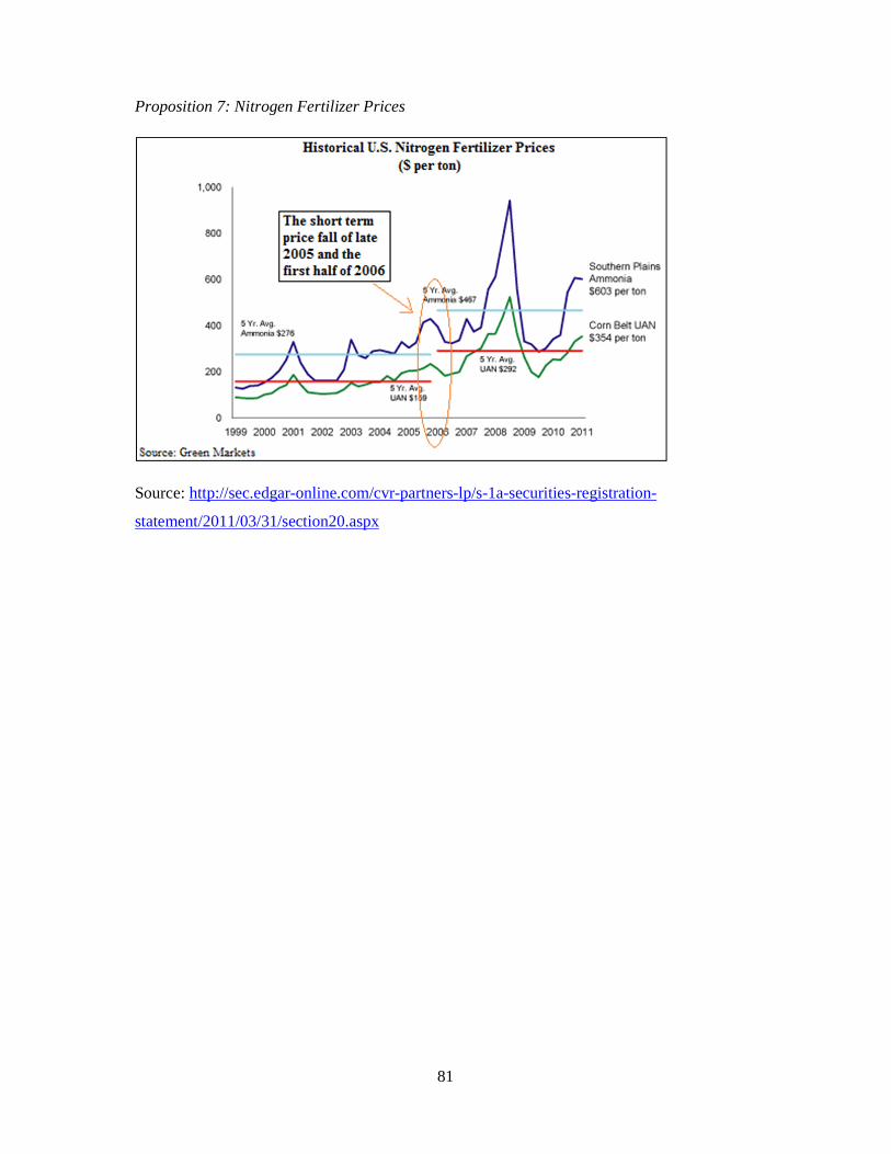
81

Proposition 7: Nitrogen Fertilizer Prices

Source: http://sec.edgar-online.com/cvr-partners-lp/s-1a-securities-registration-

statement/2011/03/31/section20.aspx

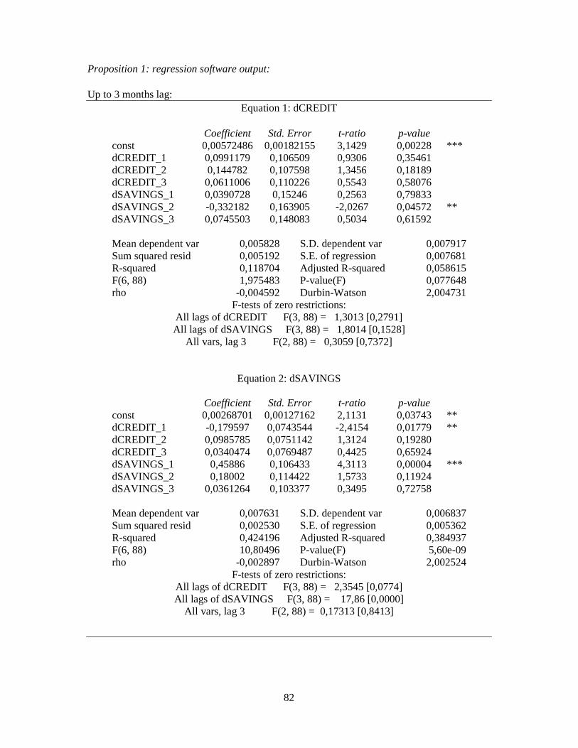
82

Proposition 1: regression software output:

Up to 3 months lag: Equation 1: dCREDIT

Coefficient Std. Error t-ratio p-value const 0,00572486 0,00182155 3,1429 0,00228 *** dCREDIT_1 0,0991179 0,106509 0,9306 0,35461 dCREDIT_2 0,144782 0,107598 1,3456 0,18189 dCREDIT_3 0,0611006 0,110226 0,5543 0,58076 dSAVINGS_1 0,0390728 0,15246 0,2563 0,79833 dSAVINGS_2 -0,332182 0,163905 -2,0267 0,04572 ** dSAVINGS_3 0,0745503 0,148083 0,5034 0,61592

Mean dependent var 0,005828 S.D. dependent var 0,007917 Sum squared resid 0,005192 S.E. of regression 0,007681 R-squared 0,118704 Adjusted R-squared 0,058615 F(6, 88) 1,975483 P-value(F) 0,077648 rho -0,004592 Durbin-Watson 2,004731

F-tests of zero restrictions: All lags of dCREDIT F(3, 88) = 1,3013 [0,2791] All lags of dSAVINGS F(3, 88) = 1,8014 [0,1528]

All vars, lag 3 F(2, 88) = 0,3059 [0,7372]

Equation 2: dSAVINGS

Coefficient Std. Error t-ratio p-value const 0,00268701 0,00127162 2,1131 0,03743 ** dCREDIT_1 -0,179597 0,0743544 -2,4154 0,01779 ** dCREDIT_2 0,0985785 0,0751142 1,3124 0,19280 dCREDIT_3 0,0340474 0,0769487 0,4425 0,65924 dSAVINGS_1 0,45886 0,106433 4,3113 0,00004 *** dSAVINGS_2 0,18002 0,114422 1,5733 0,11924 dSAVINGS_3 0,0361264 0,103377 0,3495 0,72758

Mean dependent var 0,007631 S.D. dependent var 0,006837 Sum squared resid 0,002530 S.E. of regression 0,005362 R-squared 0,424196 Adjusted R-squared 0,384937 F(6, 88) 10,80496 P-value(F) 5,60e-09 rho -0,002897 Durbin-Watson 2,002524

F-tests of zero restrictions: All lags of dCREDIT F(3, 88) = 2,3545 [0,0774] All lags of dSAVINGS F(3, 88) = 17,86 [0,0000]

All vars, lag 3 F(2, 88) = 0,17313 [0,8413]

83

Up to 5 months lag: Equation 1: dCREDIT

Coefficient Std. Error t-ratio p-value

const 0,00592039 0,00217855 2,7176 0,00802 *** dCREDIT_1 0,0972555 0,110363 0,8812 0,38077 dCREDIT_2 0,161395 0,115432 1,3982 0,16583 dCREDIT_3 0,0562436 0,118777 0,4735 0,63710 dCREDIT_4 0,01627 0,116786 0,1393 0,88954 dCREDIT_5 -0,0585937 0,116639 -0,5024 0,61677 dSAVINGS_1 0,0381912 0,157917 0,2418 0,80951 dSAVINGS_2 -0,34345 0,173447 -1,9801 0,05104 * dSAVINGS_3 0,0725985 0,179752 0,4039 0,68735 dSAVINGS_4 0,074849 0,176292 0,4246 0,67226 dSAVINGS_5 -0,0576668 0,155004 -0,3720 0,71083

Mean dependent var 0,005908 S.D. dependent var 0,007982 Sum squared resid 0,005147 S.E. of regression 0,007923 R-squared 0,121798 Adjusted R-squared 0,014700 F(10, 82) 1,137259 P-value(F) 0,345350 rho 0,004292 Durbin-Watson 1,985743

F-tests of zero restrictions: All lags of dCREDIT F(5, 82) = 0,81145 [0,5449] All lags of dSAVINGS F(5, 82) = 1,0243 [0,4089]

All vars, lag 5 F(2, 82) = 0,20981 [0,8112]

Equation 2: dSAVINGS

Coefficient Std. Error t-ratio p-value const 0,00285216 0,00149792 1,9041 0,06041 * dCREDIT_1 -0,183364 0,0758834 -2,4164 0,01790 ** dCREDIT_2 0,105965 0,0793681 1,3351 0,18553 dCREDIT_3 0,0642313 0,0816685 0,7865 0,43385 dCREDIT_4 0,0110227 0,0802996 0,1373 0,89115 dCREDIT_5 -0,106642 0,0801984 -1,3297 0,18729 dSAVINGS_1 0,457577 0,10858 4,2142 0,00006 *** dSAVINGS_2 0,175368 0,119258 1,4705 0,14526 dSAVINGS_3 0,0218121 0,123593 0,1765 0,86035 dSAVINGS_4 -0,0545427 0,121214 -0,4500 0,65392 dSAVINGS_5 0,103708 0,106577 0,9731 0,33337

Mean dependent var 0,007463 S.D. dependent var 0,006796 Sum squared resid 0,002434 S.E. of regression 0,005448 R-squared 0,427351 Adjusted R-squared 0,357516 F(10, 82) 6,119423 P-value(F) 6,71e-07 rho -0,050253 Durbin-Watson 2,099250

F-tests of zero restrictions: All lags of dCREDIT F(5, 82) = 1,7904 [0,1239] All lags of dSAVINGS F(5, 82) = 9,8578 [0,0000]

84

All vars, lag 5 F(2, 82) = 1,2716 [0,2859]

Proposition 3 regression software output: Retail:

Model 1: OLS, using observations 2001:11-2009:12 (T = 98) Dependent variable: Retail

Coefficient Std. Error t-ratio p-value

const -1,96444 0,230257 -8,5315 <0,00001 *** Credit___3_ 0,192498 0,027584 6,9786 <0,00001 *** Industry_Index 0,316465 0,0159606 19,8278 <0,00001 ***

Mean dependent var -0,600314 S.D. dependent var 2,078062 Sum squared resid 44,84887 S.E. of regression 0,687091 R-squared 0,892931 Adjusted R-squared 0,890677 F(2, 95) 396,1403 P-value(F) 8,11e-47 Log-likelihood -100,7542 Akaike criterion 207,5084 Schwarz criterion 215,2633 Hannan-Quinn 210,6451 rho 0,790093 Durbin-Watson 0,359385

Utilities:

Model 2: OLS, using observations 2001:11-2009:12 (T = 98) Dependent variable: Utilities

Coefficient Std. Error t-ratio p-value

const -2,65752 0,246919 -10,7627 <0,00001 *** Credit___3_ 0,288237 0,02958 9,7443 <0,00001 *** Industry_Index 0,316464 0,0171155 18,4898 <0,00001 ***

Mean dependent var -0,544416 S.D. dependent var 2,292056 Sum squared resid 51,57415 S.E. of regression 0,736808 R-squared 0,898793 Adjusted R-squared 0,896662 F(2, 95) 421,8357 P-value(F) 5,59e-48 Log-likelihood -107,6006 Akaike criterion 221,2012 Schwarz criterion 228,9561 Hannan-Quinn 224,3379 rho 0,821886 Durbin-Watson 0,338227

Non-durables: Model 3: OLS, using observations 2001:11-2009:12 (T = 98)

Dependent variable: Non_durables

Coefficient Std. Error t-ratio p-value const -6,42435 0,314055 -20,4561 <0,00001 ***

85

Credit___3_ 0,371071 0,0376227 9,8630 <0,00001 *** Industry_Index 0,198258 0,0217692 9,1073 <0,00001 ***

Mean dependent var -3,610259 S.D. dependent var 2,051062 Sum squared resid 83,43264 S.E. of regression 0,937144 R-squared 0,795541 Adjusted R-squared 0,791236 F(2, 95) 184,8202 P-value(F) 1,79e-33 Log-likelihood -131,1705 Akaike criterion 268,3410 Schwarz criterion 276,0959 Hannan-Quinn 271,4777 rho 0,893847 Durbin-Watson 0,213657

Wholesale:

Model 4: OLS, using observations 2001:11-2009:12 (T = 98) Dependent variable: Wholesale

Coefficient Std. Error t-ratio p-value

const -3,32178 0,331037 -10,0345 <0,00001 *** Credit___3_ 0,389042 0,0396571 9,8101 <0,00001 *** Industry_Index 0,346183 0,0229464 15,0866 <0,00001 ***

Mean dependent var -0,433385 S.D. dependent var 2,729421 Sum squared resid 92,69969 S.E. of regression 0,987819 R-squared 0,871718 Adjusted R-squared 0,869017 F(2, 95) 322,7781 P-value(F) 4,34e-43 Log-likelihood -136,3315 Akaike criterion 278,6629 Schwarz criterion 286,4178 Hannan-Quinn 281,7996 rho 0,860590 Durbin-Watson 0,290003

Durables:

Model 5: OLS, using observations 2001:11-2009:12 (T = 98) Dependent variable: Durables

Coefficient Std. Error t-ratio p-value

const -10,0713 0,750063 -13,4273 <0,00001 *** Credit___3_ 0,77223 0,0898548 8,5942 <0,00001 *** Industry_Index 0,524678 0,0519917 10,0916 <0,00001 ***

Mean dependent var -4,265192 S.D. dependent var 4,843214 Sum squared resid 475,9044 S.E. of regression 2,238196 R-squared 0,790839 Adjusted R-squared 0,786436 F(2, 95) 179,5978 P-value(F) 5,28e-33 Log-likelihood -216,4882 Akaike criterion 438,9764 Schwarz criterion 446,7313 Hannan-Quinn 442,1131 rho 0,906046 Durbin-Watson 0,191835

Construction:

Model 6: OLS, using observations 2001:11-2009:12 (T = 98) Dependent variable: Construction

86

Coefficient Std. Error t-ratio p-value const -4,76379 1,12155 -4,2475 0,00005 *** Credit___3_ 0,495597 0,134357 3,6886 0,00038 *** Industry_Index 0,968931 0,0777418 12,4634 <0,00001 ***

Mean dependent var -1,320862 S.D. dependent var 6,695861 Sum squared resid 1064,045 S.E. of regression 3,346711 R-squared 0,755333 Adjusted R-squared 0,750182 F(2, 95) 146,6414 P-value(F) 9,06e-30 Log-likelihood -255,9144 Akaike criterion 517,8288 Schwarz criterion 525,5837 Hannan-Quinn 520,9655 rho 0,925503 Durbin-Watson 0,146280

Mining & Logging:

Model 7: OLS, using observations 2001:11-2009:12 (T = 98) Dependent variable: MiningNLodging

Coefficient Std. Error t-ratio p-value

const -9,45867 1,34918 -7,0107 <0,00001 *** Credit___3_ 1,45657 0,161627 9,0119 <0,00001 *** Industry_Index 0,188503 0,0935207 2,0156 0,04666 **

Mean dependent var 1,851808 S.D. dependent var 6,280020 Sum squared resid 1539,808 S.E. of regression 4,025979 R-squared 0,597494 Adjusted R-squared 0,589020 F(2, 95) 70,51054 P-value(F) 1,69e-19 Log-likelihood -274,0238 Akaike criterion 554,0476 Schwarz criterion 561,8025 Hannan-Quinn 557,1843 rho 0,923003 Durbin-Watson 0,152086

Collinearity test: Variance Inflation Factors Minimum possible value = 1.0 Values > 10.0 may indicate a collinearity problem Credit___3_ 1,357 Industry_Index 1,357 VIF(j) = 1/(1 - R(j)^2), where R(j) is the multiple correlation coefficient between variable j and the other independent variables Properties of matrix X'X: 1-norm = 8009,3551 Determinant = 1,5292551e+008 Reciprocal condition number = 0,00096701994