IMES DISCUSSION PAPER SERIES

INSTITUTE FOR MONETARY AND ECONOMIC STUDIES

BANK OF JAPAN

2-1-1 NIHONBASHI-HONGOKUCHO

CHUO-KU, TOKYO 103-8660

JAPAN

You can download this and other papers at the IMES Web site:

https://www.imes.boj.or.jp

Do not reprint or reproduce without permission.

Speed Limit Policy and Liquidity Traps

Taisuke Nakata, Sebastian Schmidt, and Paul Yoo

Discussion Paper No. 2018-E-6

NOTE: IMES Discussion Paper Series is circulated in

order to stimulate discussion and comments. Views

expressed in Discussion Paper Series are those of

authors and do not necessarily reflect those of

the Bank of Japan or the Institute for Monetary

and Economic Studies.

IMES Discussion Paper Series 2018-E-6

June 2018

Speed Limit Policy and Liquidity Traps

Taisuke Nakata*, Sebastian Schmidt**, and Paul Yoo***

Abstract

The zero lower bound (ZLB) constraint on interest rates makes speed limit policies

(SLPs)－policies aimed at stabilizing the output growth－less effective. Away

from the ZLB, the history dependence induced by a concern for output growth

stabilization improves the inflation-output tradeoff for a discretionary central bank.

However, in the aftermath of a deep recession with a binding ZLB, a central bank

with an objective for output growth stabilization aims to engineer a more gradual

increase in output than under the standard discretionary policy. The anticipation of

a more restrained recovery exacerbates the declines in inflation and output when

the lower bound is binding.

Keywords: Liquidity Traps; Markov-Perfect Equilibrium; Speed Limit Policy;

Zero Lower Bound

JEL classification: E52, E61

*Board of Governors of the Federal Reserve System (E-mail: taisuke.nakata@frb.gov)

**European Central Bank (E-mail: sebastian.schmidt@ecb.int)

***UNC Kenan-Flagler Business School (E-mail: paul_yoo@kenan-flagler.unc.edu)

This paper was prepared in part while Taisuke Nakata was a visiting scholar at the Institute for

Monetary and Economic Studies, Bank of Japan. The authors thank seminar participants at the

Bank of Japan and the University of Tokyo for comments and suggestions. The authors also

thank Shigenori Shiratsuka, Yoichi Ueno, and an anonymous referee for the IMES Discussion

Paper Series for useful suggestions and Katherine Arnold for editorial assistance. Philip Coyle,

Philipp Lieberknecht, and Jonathan Yu provided excellent research assistance. The views

expressed in this paper are those of the authors and do not necessarily reflect the official views

of the Bank of Japan, the Federal Reserve Board of Governors, the Federal Reserve System, or

the European Central Bank.

1 Introduction

Economists have long studied the efficacies of various monetary policy strategies. Several

studies on the design of monetary policy have emphasized the desirability of central bank

objectives that assign a role to the stabilization of output growth. First and foremost,

a seminal paper by Walsh (2003) demonstrated that, in standard sticky-price models, a

discretionary central bank that is concerned with stabilization of inflation and output growth,

rather than output, improves welfare by creating endogenous inertia in the interest rate

policy that is akin to the inertia observed under the optimal commitment policy. Others

made a similar point by showing that interest rate feedback rules involving an output growth

stabilization term can generate economic outcomes similar to those achieved under optimal

commitment policy in various sticky-price models (Blake (2012); Giannoni and Woodford

(2003); Stracca (2007)). These policies that aim to reduce output growth volatility are

known as speed limit policies (SLPs).

In this paper, we revisit the desirability of SLPs in an economy with an occasionally

binding zero lower bound (ZLB) constraint on nominal interest rates. Following Walsh (2003),

we conduct our analyses in the context of policy delegation where the discretionary central

bank’s objective function is modified to include an output growth stabilization motive.1 Our

model features both demand and cost-push shocks. In the model without the ZLB constraint,

the presence of the cost-push shock makes it desirable to assign a strictly positive weight to

the output growth stabilization motive, as shown by Walsh (2003). The presence of the

demand shock would have no implication for the desirability of SLPs when we abstract from

the ZLB constraint because the demand shock can be fully neutralized by the adjustment in

the policy rate regardless of whether or not the central bank pursues a SLP. However, in the

model with the ZLB, a sufficiently large negative demand shock forces the central bank to

reduce the policy rate to the ZLB, causing inflation and the output gap to decline. In this

case, demand disturbances are no longer inconsequential for the assessment of SLPs.

Our main exercise is to compare the desirability of SLPs in the models with and without

the ZLB constraint. We begin our analysis with a stylized model in which the cost and benefit

of the SLP can be transparently described. We then move on to a richer model calibrated to

match key features of the U.S. economy to examine the quantitative relevance of SLP.

Our main finding is that the optimal weight on the output growth stabilization term is

smaller in the model with the ZLB constraint than in the model that abstracts from the

constraint. The ZLB constraint makes SLPs less desirable because the central bank under a

SLP acts in a way that is almost a polar opposite of what the central bank would do under

the optimal commitment policy. Under the optimal commitment policy, the central bank

1A key insight of the literature on policy delegation is that delegating policy to an agent with a differentobjective function than society can help to solve time inconsistency problems and improve welfare. Prominentexamples in the context of monetary policy include Rogoff (1985), Persson and Tabellini (1993), Walsh (1995),Walsh (2003), and Svensson (1997).

1

keeps the policy rate low for long with the explicit goal of overshooting inflation and the

output gap above their longer-run targets. The overshooting of inflation and the output gap

in the future mitigates the declines in inflation and the output gap while the ZLB is a binding

constraint through improved expectations.

Under the SLP, the central bank has an incentive to raise the policy rate more rapidly in

the aftermath of a crisis than it does under the standard discretionary policy in order to keep

the output gap close to the low level that prevailed during the crisis. Since households and

firms are forward-looking, the expectations of low output gap and low inflation associated

with it amplify the declines in inflation and the output gap at the ZLB constraint.

The extent to which the ZLB constraint reduces the optimal weight on the output growth

stabilization term depends on the specifics of the model under investigation. In the stylized

model, the optimal weight on the output growth term becomes smaller when the ZLB con-

straint is accounted for, but remains strictly positive under all parameter values we consider

in this paper. In the quantitative model calibrated to match key features of the U.S. economy,

we find that the optimal weight is zero in the model with the ZLB, while it is positive in the

model without the ZLB.

This paper builds on previous studies that have examined the desirability of SLPs in

sticky-price models. As mentioned in the introductory paragraph, the benefits of SLPs

arising from its ability to generate desirable history dependence in the policy rate have

been documented by several studies (Blake (2012); Giannoni and Woodford (2003); Stracca

(2007); Walsh (2003)).2 Others have emphasized the desirability of SLP in models where

the target variable—be it the output gap or unemployment gap—is measured with errors.

Examples are Orphanides, Porter, Reifschneider, Tetlow, and Finan (2000), Orphanides and

Williams (2002), and Orphanides and Williams (2007). In such models with measurement

errors, policies aimed at reducing the volatility of the mismeasured target variable can cause

a higher-than-intended volatility in the policy rate, which in turn leads to higher volatilities

of inflation and the output gap. All these papers, however, abstract from the ZLB constraint:

our contribution is to examine the desirability of speed-limit policy in models with the ZLB

constraint.

The message of our paper echoes those of Blake, Kirsanova, and Yates (2013) and Brendon,

Paustian, and Yates (2013) which provide caveats to speed-limit policies in different setups.

Blake, Kirsanova, and Yates (2013) show that, when a persistent endogenous variable—such

as capital—is introduced into an otherwise standard New Keynesian model without the ZLB,

there are multiple equilibria under the standard discretionary policy. They find that SLPs

often improve welfare in one equilibrium, but worsen welfare in another. Brendon, Paustian,

and Yates (2013) examine the desirability of adding an output growth stabilization term in an

interest rate feedback rule in the New Keynesian model with the ZLB constraint. They find

that the combination of SLP and the ZLB constraint can generate belief-driven recessions.

2See Bilbiie (2014) and Bodenstein and Zhao (2017) for more recent contributions.

2

Our analysis is different from Blake, Kirsanova, and Yates (2013) because our result does not

require the presence of any natural endogenous state variables and our analysis features the

ZLB constraint. Our analysis differs from Brendon, Paustian, and Yates (2013) because we

assume the central bank is optimizing, as opposed to following an interest-rate feedback rule,

and we focus on recessions driven by fundamental shocks.

Finally, this paper is related to a set of papers that consider policy delegation approaches

to mitigate the adverse consequences of the ZLB under the discretionary central bank. Nakata

and Schmidt (2014) demonstrate that the appointment of an inflation-conservative central

banker is welfare-improving, as it mitigates the deflationary bias problem facing the discre-

tionary central bank in the economy with occasionally binding ZLB constraint. Billi (2013)

shows that modifying the central bank’s objective function to include a nominal-income

stabilization objective or a price-level stabilization objective can improve welfare, as both

frameworks generate a form of history dependence that is similar to the history dependence

attained under the optimal commitment policy. Finally, Nakata and Schmidt (2016) show

that it is welfare-improving to assign an interest rate smoothing objective to the central

bank, as the desire to smooth the path of interest rates creates a desirable history depen-

dence, leading the central bank to keep the policy rate low for long in the aftermath of a

recession. Our work is a useful reminder that introducing history dependence per se does not

improve welfare; one needs the right kind of history dependence.

As the U.S. economy and monetary policy normalize, there is a growing interest in re-

examining monetary policy strategies when the policy rate is subject to the ZLB (see, for

example, Williams (2017)). Accordingly, a careful re-examination of how policy strategies

known to perform well in the economy without ZLB would perform once the ZLB is taken

into account is as relevant as ever. Although there are a growing number of papers on this

question of how to best conduct monetary policy in the presence of the ZLB constraint, so

far there is no paper examining how SLP performs in the model with ZLB. Thus, our paper

fills in an important gap in the literature.

The rest of the paper is organized as follows. Section 2 describes the stylized model

and formulates the problem or the central bank. Section 3 presents the results on how the

ZLB constraint alters the desirability of SLPs. Section 4 extends the analysis to a calibrated

quantitative model. Section 5 examines the the desirability of SLPs in the context of modified

interest rate feedback rules. Section 6 concludes.

2 The model

This section presents the model, lays down the policy problem of the central bank and defines

the equilibrium.

3

2.1 Private sector

The private sector of the economy is given by the standard New Keynesian structure formu-

lated in discrete time with infinite horizon as described in detail in Woodford (2003) and Gali

(2015). A continuum of identical, infinitely-living households consumes a basket of differen-

tiated goods and supplies labor in a perfectly competitive labor market. The consumption

goods are produced by firms using (industry-specific) labor. Firms maximize profits subject

to staggered price-setting as in Calvo (1983). Following the majority of the literature on the

ZLB, we put all model equations except for the ZLB constraint in semi-loglinear form.

The equilibrium conditions of the private sector are given by the following two equations:

πt = κyt + βEtπt+1 + et (1)

yt = Etyt+1 − σ (it − Etπt+1 − rnt ) , (2)

where πt is the inflation rate between periods t − 1 and t, yt denotes the output gap, it is

the level of the nominal interest rate between periods t and t+ 1, rnt is an exogenous natural

real rate of interest, and et is an exogenous cost-push shock.. Equation (1) is a standard

New Keynesian Phillips curve and equation (2) is the Euler equation. Parameters satisfy

β ∈ (0, 1) and σ, κ > 0.3

We assume that the natural real rate follows a two-state Markov process. In particular,

rnt takes the value of either rnH or rnL where we refer to rnH > 0 as the high (non-crisis) state

and rnL < 0 as the low (crisis) state. The transition probabilities are given by

Prob(rnt+1 = rnL|rnt = rnH) = pH (3)

Prob(rnt+1 = rnL|rnt = rnL) = pL. (4)

pH is the probability of moving to the low state in the next period when the economy is in

the high state today and will be referred to as the frequency of the contractionary shocks.

pL is the probability of staying in the low state when the economy is in the low state today

and will be referred to as the persistence of the contractionary shocks. We will also refer to

high and low states as non-crisis and crisis states, respectively.

We assume that the cost-push shock et follows a three-state Markov process, taking eH ,

eM , and eL. For simplicity, we now assume that the process is independent and the probability

of each state is identical. In other words, Prob(et+1 = ei|et = ej) = 1/3 for any i and j in

{H,M,L}. For simplicity, we also assume the shock is symmetric in size. That is, eH = c,

eM = 0, and eL = −c where c is the magnitude of the cost-push shock. In Appendix A, we

show the robustness of our result in a version of the stylized model in which the demand and

cost-push shocks follow AR(1) processes.

3κ is related to the structural parameters of the economy as follows: κ = (1−α)(1−αβ)α(1+ηθ)

(σ−1 + η

), where

α ∈ (0, 1) denotes the share of firms that cannot reoptimize their price in a given period, η > 0 is the inverseof the elasticity of labor supply, and θ > 1 denotes the price elasticity of demand for differentiated goods.

4

2.2 Society’s objective and the central bank’s problem

We assume that society’s value, or welfare, at time t is given by the expected discounted sum

of future utility flows,

Vt = u(πt, yt) + βEtVt+1, (5)

where society’s contemporaneous utility function, u(·, ·), is given by the standard quadratic

function of inflation and the output gap,

u(π, y) = −1

2

(π2 + λy2

). (6)

This objective function can be motivated by a second-order approximation to the household’s

preferences. In such a case, λ is a function of the structural parameters and is given by

λ = κ/θ.

The value for the central bank is given by

V CBt = uCB(πt, yt, yt−1) + βEtV CB

t+1 . (7)

where the central bank’s contemporaneous utility function, uCB(·, ·), is given by

uCB(πt, yt, yt−1) = −1

2

(π2t + λy2

t + α(yt − yt−1)2). (8)

Note that the central bank’s objective function has the output growth stabilization term

α(yt − yt−1)2 in addition to the inflation and output stabilization terms.4 We assume that

the central bank does not have a commitment technology. When α = 0, the central bank’s

contemporaneous utility function is identical to that of the society. We will refer to the

optimal discretionary policy associated with α = 0 as the standard discretionary policy.

Each period t, the central bank chooses the inflation rate, the output gap, and the nominal

interest rate in order to maximize its objective function subject to the behavioral constraints

of the private sector, with the policy functions at time t+ 1 taken as given. The problem of

the central bank is thus given by

V CBt (rnt , yt−1) = max

πt,yt,ituCB(πt, yt, yt−1) + βEtV CB

t+1 (rnt+1, yt). (9)

subject to the ZLB constraint,

it ≥ 0, (10)

and the private-sector equilibrium conditions (1) and (2) described above.

A Markov-Perfect equilibrium is defined as a set of time-invariant value and policy func-

tions {V CB(·, ·), y(·, ·), π(·, ·), i(·, ·)} that solves the central bank’s problem above, together

4In Walsh (2003), the central bank’s objective function is modified so that the output growth stabilizationterm replaces the output stabilization term. We choose to keep the output stabilization term because, bydoing so, the central bank’s objective function nests the society’s objective function and thus the mechanismis clear.

5

with society’s value function V (·, ·), which is consistent with y(·, ·) and π(·, ·).The main exercise of the paper will be to examine the effects of α on welfare. We quantify

the welfare of an economy by the perpetual consumption transfer (as a share of its steady

state) that would make a household in the economy indifferent to living in the economy

without any fluctuations. This is given by

W := (1− β)θ

κ

(σ−1 + η

)E[V ]. (11)

where the mathematical expectation is taken with respect to the unconditional distribution

of dt and yt−1.

2.3 Parameter values and solution methods

Parameter values for the stylized model are shown in Table 1. The values for the model’s

behavioral parameters are from Woodford (2003). The parameters governing the shock pro-

cesses are chosen to illustrate the key forces of the model in a transparent way. We will

conduct sensitivity analyses with respect to key parameters at the end of Section 3.

Table 1: Parameter Values for the Stylized Model

Parameter Value Economic interpretation

β 0.99 Subjective discount factorσ 1 Interest-rate elasticity of outputκ 0.024 Slope of the Phillips curveλ 0.003 Weight on the output stabilization termrnH 0.01 Natural-rate shock in the high staternL -0.015 Natural-rate shock in the low statepH 0.005 Frequency of contractionary demand shockpL 0.5 Persistence of contractionary demand shock100c 0.15 Magnitude of cost-push shocks

We solve the model by a variant of the standard time-iteration method that is modified to

take it into consideration that the partial derivatives of future policy show up in the system

of nonlinear equations characterizing the model’s equilibrium conditions. The details of the

solution method and the solution accuracy are described in Appendix B and C, respectively.

3 Results

This section describes how the introduction of an output growth objective affects welfare and

the propagation of economic shocks in the models with and without the ZLB.

6

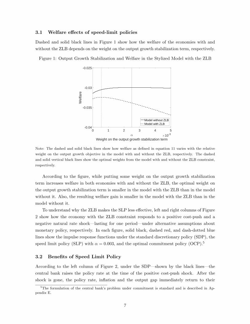
3.1 Welfare effects of speed-limit policies

Dashed and solid black lines in Figure 1 show how the welfare of the economies with and

without the ZLB depends on the weight on the output growth stabilization term, respectively.

Figure 1: Output Growth Stabilization and Welfare in the Stylized Model with the ZLB

0 1 2 3 4 5

α

Weight on the output growth stabilization term×10

-3

-0.04

-0.035

-0.03

-0.025

Welfare

Model without ZLB

Model with ZLB

Note: The dashed and solid black lines show how welfare as defined in equation 11 varies with the relative

weight on the output growth objective in the model with and without the ZLB, respectively. The dashed

and solid vertical black lines show the optimal weights from the model with and without the ZLB constraint,

respectively.

According to the figure, while putting some weight on the output growth stabilization

term increases welfare in both economies with and without the ZLB, the optimal weight on

the output growth stabilization term is smaller in the model with the ZLB than in the model

without it. Also, the resulting welfare gain is smaller in the model with the ZLB than in the

model without it.

To understand why the ZLB makes the SLP less effective, left and right columns of Figure

2 show how the economy with the ZLB constraint responds to a positive cost-push and a

negative natural rate shock—lasting for one period—under alternative assumptions about

monetary policy, respectively. In each figure, solid black, dashed red, and dash-dotted blue

lines show the impulse response functions under the standard discretionary policy (SDP), the

speed limit policy (SLP) with α = 0.003, and the optimal commitment policy (OCP).5

3.2 Benefits of Speed Limit Policy

According to the left column of Figure 2, under the SDP—shown by the black lines—the

central bank raises the policy rate at the time of the positive cost-push shock. After the

shock is gone, the policy rate, inflation and the output gap immediately return to their

5The formulation of the central bank’s problem under commitment is standard and is described in Ap-pendix E.

7

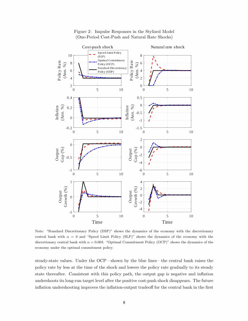
Figure 2: Impulse Responses in the Stylized Model(One-Period Cost-Push and Natural Rate Shocks)

0 5 102

4

6

8

10P

olic

y R

ate

(Ann. %

)

Cost-push shock

Speed-Limit Policy

(SLP)

Optimal Commitment

Policy (OCP)

Standard Discretionary

Policy (SDP)

0 5 100

2

4

6

8

Polic

y R

ate

(Ann. %

)

Natural rate shock

0 5 10-0.2

0

0.2

0.4

Inflation

(Ann. %

)

0 5 10-1.5

-1

-0.5

0

0.5

Inflation

(Ann. %

)

0 5 10-1

-0.5

0

Outp

ut

Gap (

%)

0 5 10-6

-4

-2

0

2

Outp

ut

Gap (

%)

0 5 10

Time

-1

0

1

Outp

ut

Gro

wth

(%

)

0 5 10

Time

-4

-2

0

2

4

Outp

ut

Gro

wth

(%

)

Note: “Standard Discretionary Policy (DSP)” shows the dynamics of the economy with the discretionary

central bank with α = 0 and “Speed Limit Policy (SLP)” shows the dynamics of the economy with the

discretionary central bank with α = 0.003. “Optimal Commitment Policy (OCP)” shows the dynamics of the

economy under the optimal commitment policy.

steady-state values. Under the OCP—shown by the blue lines—the central bank raises the

policy rate by less at the time of the shock and lowers the policy rate gradually to its steady

state thereafter. Consistent with this policy path, the output gap is negative and inflation

undershoots its long-run target level after the positive cost-push shock disappears. The future

inflation undershooting improves the inflation-output tradeoff for the central bank in the first

8

period through expectations. As a result, both the rise in inflation and the fall in the output

gap in the initial period are smaller under the OCP than under the SDP. The benefit of

more stable inflation and output in the first period dominates the less-stabilized inflation

and output afterwards in terms of welfare. This welfare gain from policy commitment in

sticky-price models with a cost-push shock is well known in the literature (Woodford (2003)

and Gali (2015)).

Under the SLP—shown by the red lines—the policy rate path is qualitatively similar to

that under the OCP; the central bank raises the policy rate initially by less than it would

under the standard discretionary policy and lowers it gradually to its steady-state value

afterwards. Output declines less than under the SDP in the first period and gradually returns

to its steady state. This path of the output gap leads to a small temporary undershooting

of inflation from the second period on, with the initial increase in inflation being about

the same as that under the standard discretionary policy. With the inflation path roughly

unchanged from the SDP, but the output gap path substantially more stabilized, the welfare

costs associated with cost-push shocks are smaller under the SLP than under the SDP. This

beneficial effect of the SLP in response to a cost-push shock was first pointed out by Walsh

(2003) and is present in both the model with the ZLB and the model without the ZLB.

3.3 Costs of Speed Limit Policy

We now turn to the right column of Figure 2 which shows how the economy with the ZLB

responds to a negative demand shock. Under the SDP—shown by the black lines—the central

bank keeps the policy rate at the ZLB as long as the crisis shock lasts, and inflation and output

return to their steady-state values immediately after the crisis shock disappears. Under the

OCP—shown by the blue lines—the central bank keeps the policy rate at the ZLB for two

extra periods after the crisis shock is gone, which generates a temporary overshooting of

inflation and output above their long-run targets. Since households and firms are forward-

looking, the anticipation of the overshooting mitigates the declines in inflation and output

while the policy rate is constrained at the ZLB. These dynamics of the economy under the

SDP and the OCP just described have been studied by many, most notably by Eggertsson

and Woodford (2003).

Under the SLP—shown by the blue lines—the policy rate path in the aftermath of a crisis

shock is almost a mirror image of what prevails under the OCP: The central bank under the

SLP raises the policy rate above its steady-state level after the crisis shock disappears in order

to let output return gradually to its steady-state level. As a result, inflation also returns to its

steady state gradually. Through expectations, more gradual returns of inflation and output

exacerbate the initial declines in inflation and output when the ZLB is a binding constraint.

Ironically, in equilibrium, the output growth term is less stabilized under the SLP than under

the SDP, as shown by the bottom-right panel.

Note that, in the absence of the ZLB constraint, output and inflation are fully stabilized

9

in the presence of a demand shock under the SDP, the OCP, and the SLP. Thus, it is the

interaction of the ZLB constraint and a large negative shock that makes SLP undesirable.

3.4 Sensitivity Analysis

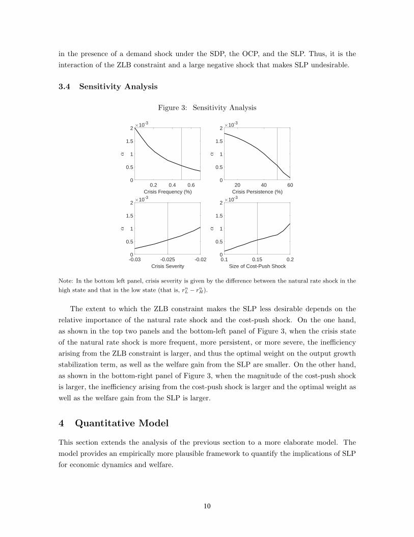
Figure 3: Sensitivity Analysis

0.2 0.4 0.6

Crisis Frequency (%)

0

0.5

1

1.5

210

-3

20 40 60

Crisis Persistence (%)

0

0.5

1

1.5

210

-3

-0.03 -0.025 -0.02

Crisis Severity

0

0.5

1

1.5

210

-3

0.1 0.15 0.2

Size of Cost-Push Shock

0

0.5

1

1.5

210

-3

Note: In the bottom left panel, crisis severity is given by the difference between the natural rate shock in the

high state and that in the low state (that is, rnL − rnH).

The extent to which the ZLB constraint makes the SLP less desirable depends on the

relative importance of the natural rate shock and the cost-push shock. On the one hand,

as shown in the top two panels and the bottom-left panel of Figure 3, when the crisis state

of the natural rate shock is more frequent, more persistent, or more severe, the inefficiency

arising from the ZLB constraint is larger, and thus the optimal weight on the output growth

stabilization term, as well as the welfare gain from the SLP are smaller. On the other hand,

as shown in the bottom-right panel of Figure 3, when the magnitude of the cost-push shock

is larger, the inefficiency arising from the cost-push shock is larger and the optimal weight as

well as the welfare gain from the SLP is larger.

4 Quantitative Model

This section extends the analysis of the previous section to a more elaborate model. The

model provides an empirically more plausible framework to quantify the implications of SLP

for economic dynamics and welfare.

10

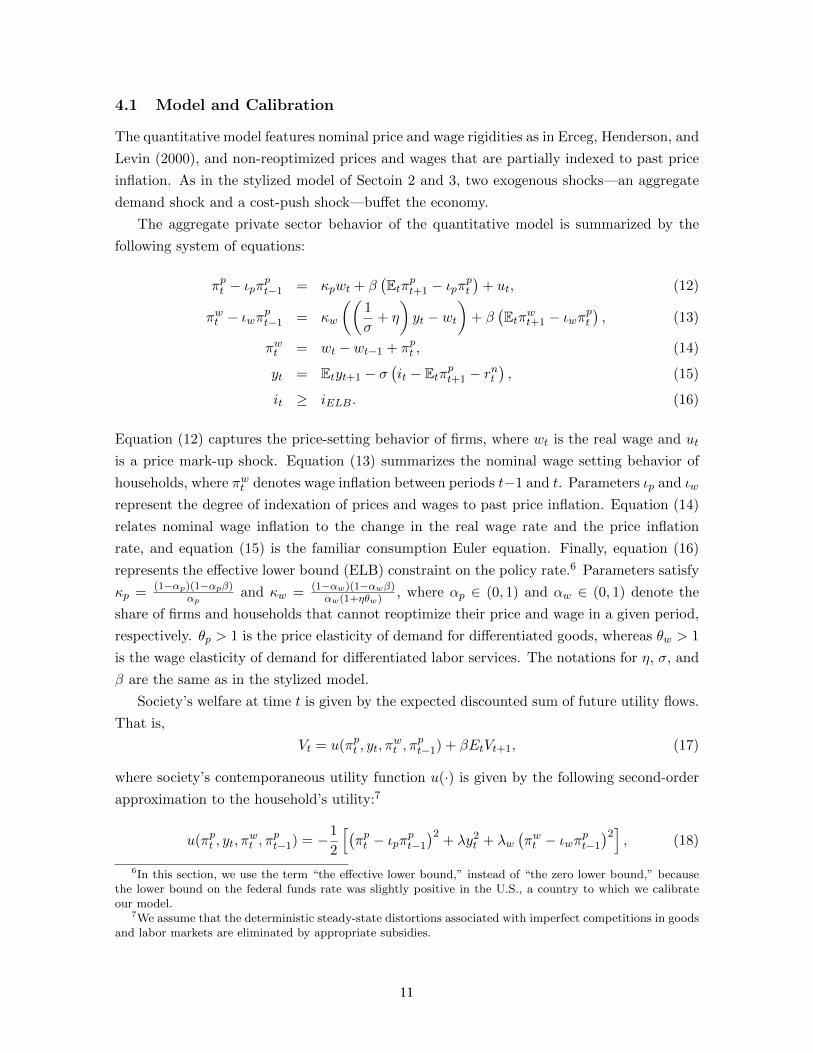
4.1 Model and Calibration

The quantitative model features nominal price and wage rigidities as in Erceg, Henderson, and

Levin (2000), and non-reoptimized prices and wages that are partially indexed to past price

inflation. As in the stylized model of Sectoin 2 and 3, two exogenous shocks—an aggregate

demand shock and a cost-push shock—buffet the economy.

The aggregate private sector behavior of the quantitative model is summarized by the

following system of equations:

πpt − ιpπpt−1 = κpwt + β

(Etπpt+1 − ιpπ

pt

)+ ut, (12)

πwt − ιwπpt−1 = κw

((1

σ+ η

)yt − wt

)+ β

(Etπwt+1 − ιwπ

pt

), (13)

πwt = wt − wt−1 + πpt , (14)

yt = Etyt+1 − σ(it − Etπpt+1 − r

nt

), (15)

it ≥ iELB. (16)

Equation (12) captures the price-setting behavior of firms, where wt is the real wage and ut

is a price mark-up shock. Equation (13) summarizes the nominal wage setting behavior of

households, where πwt denotes wage inflation between periods t−1 and t. Parameters ιp and ιw

represent the degree of indexation of prices and wages to past price inflation. Equation (14)

relates nominal wage inflation to the change in the real wage rate and the price inflation

rate, and equation (15) is the familiar consumption Euler equation. Finally, equation (16)

represents the effective lower bound (ELB) constraint on the policy rate.6 Parameters satisfy

κp =(1−αp)(1−αpβ)

αpand κw = (1−αw)(1−αwβ)

αw(1+ηθw) , where αp ∈ (0, 1) and αw ∈ (0, 1) denote the

share of firms and households that cannot reoptimize their price and wage in a given period,

respectively. θp > 1 is the price elasticity of demand for differentiated goods, whereas θw > 1

is the wage elasticity of demand for differentiated labor services. The notations for η, σ, and

β are the same as in the stylized model.

Society’s welfare at time t is given by the expected discounted sum of future utility flows.

That is,

Vt = u(πpt , yt, πwt , π

pt−1) + βEtVt+1, (17)

where society’s contemporaneous utility function u(·) is given by the following second-order

approximation to the household’s utility:7

u(πpt , yt, πwt , π

pt−1) = −1

2

[(πpt − ιpπ

pt−1

)2+ λy2

t + λw(πwt − ιwπ

pt−1

)2], (18)

6In this section, we use the term “the effective lower bound,” instead of “the zero lower bound,” becausethe lower bound on the federal funds rate was slightly positive in the U.S., a country to which we calibrateour model.

7We assume that the deterministic steady-state distortions associated with imperfect competitions in goodsand labor markets are eliminated by appropriate subsidies.

11

The relative weights are functions of the structural parameters.8

The central bank acts under discretion. The central bank’s contemporaneous utility

function uCB(·) is given by,

uCB(πpt , yt, yt−1, πwt , π

pt−1) = −1

2

{(1− α)

[(πpt − ιpπ

pt−1

)2+ λy2

t + λw(πwt − ιwπ

pt−1

)2]+α(yt − yt−1)2

}, (19)

where α ≥ 0 is the weight on the output growth stabilization term. When α = 0, the central

bank’s objective function collapses to society’s objective function.

Each period t, the central bank chooses the price and wage inflation rate, the output gap,

the real wage, and the nominal interest rate to maximize its objective function subject to the

private-sector equilibrium conditions (equations (12) - (16)) and the ELB constraint, with

the value and policy functions at time t+ 1 taken as given,

V CBt (ut, r

nt , yt−1, π

pt−1, wt−1) = max

πpt ,πwt ,yt,wt,it

uCB(πpt , yt, yt−1, πwt , π

pt−1)

+ βEtV CBt+1 (ut+1, r

nt+1, yt, π

pt , wt). (20)

The first-order necessary conditions are presented in Appendix D.

We quantify the effects of gradualism on society’s welfare by the perpetual consumption

transfer (as a share of its steady state) that would make a household in the artificial economy

without any fluctuations indifferent to living in the economy just described. This welfare-

equivalent consumption transfer is given by

W := (1− β)θpκpE[V ]. (21)

Parameter values, shown in Table 2, are chosen so that the key moments implied by the

model under α = 0 are in line with those in the U.S. economy over the last two decades. The

model-implied standard deviations of inflation, output, and the policy rate are 0.63 percent

(annualized), 2.9 percent, and 2.3 percent. The same moments from the U.S. data are 0.52

percent (annualized), 2.8 percent, and 2.2 percent.9 The model-implied probability of being

at the ELB is about 28 percent, while the federal funds rate was at the ELB constraint 35

percent of the time over the past two decades.

8Specifically, λ = κp(1σ

+ η)

1θp

and λw = λ θwκw( 1

σ+η)

.9Our sample is from 1997:Q3 to 2017:Q2. Inflation rate is computed as the annualized quarterly percentage

change (log difference) in the personal consumption expenditure core price index. The measure of the outputgap is based on the FRB/US model. The quarterly average of the (annualized) federal funds rate is used asthe measure for the policy rate.

12

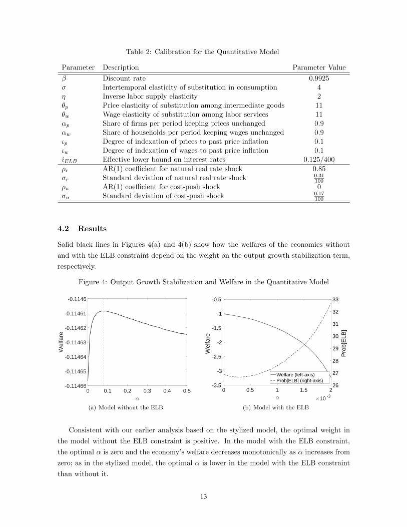
Table 2: Calibration for the Quantitative Model

Parameter Description Parameter Value

β Discount rate 0.9925σ Intertemporal elasticity of substitution in consumption 4η Inverse labor supply elasticity 2θp Price elasticity of substitution among intermediate goods 11θw Wage elasticity of substitution among labor services 11αp Share of firms per period keeping prices unchanged 0.9αw Share of households per period keeping wages unchanged 0.9ιp Degree of indexation of prices to past price inflation 0.1ιw Degree of indexation of wages to past price inflation 0.1iELB Effective lower bound on interest rates 0.125/400

ρr AR(1) coefficient for natural real rate shock 0.85σr Standard deviation of natural real rate shock 0.31

100ρu AR(1) coefficient for cost-push shock 0σu Standard deviation of cost-push shock 0.17

100

4.2 Results

Solid black lines in Figures 4(a) and 4(b) show how the welfares of the economies without

and with the ELB constraint depend on the weight on the output growth stabilization term,

respectively.

Figure 4: Output Growth Stabilization and Welfare in the Quantitative Model

0 0.1 0.2 0.3 0.4 0.5

α

-0.11466

-0.11465

-0.11464

-0.11463

-0.11462

-0.11461

-0.1146

Welfare

(a) Model without the ELB

0 0.5 1 1.5 2

10-3

-3.5

-3

-2.5

-2

-1.5

-1

-0.5

We

lfa

re

26

27

28

29

30

31

32

33

Pro

b[E

LB

]

Welfare (left-axis)

Prob[ELB] (right-axis)

(b) Model with the ELB

Consistent with our earlier analysis based on the stylized model, the optimal weight in

the model without the ELB constraint is positive. In the model with the ELB constraint,

the optimal α is zero and the economy’s welfare decreases monotonically as α increases from

zero; as in the stylized model, the optimal α is lower in the model with the ELB constraint

than without it.

13

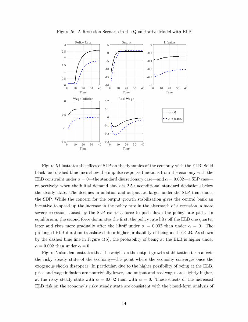
Figure 5: A Recession Scenario in the Quantitative Model with ELB

0 10 20 30 40

Time

0

0.5

1

1.5

2

2.5

3Policy Rate

α = 0

α = 0.002

0 10 20 30 40

Time

-20

-15

-10

-5

0

5Output

0 10 20 30 40

Time

-1

-0.8

-0.6

-0.4

-0.2

0Inflation

0 10 20 30 40

Time

-1.5

-1

-0.5

0Wage Inflation

0 10 20 30 40

Time

-0.3

-0.2

-0.1

0

0.1

0.2Real Wage

Figure 5 illustrates the effect of SLP on the dynamics of the economy with the ELB. Solid

black and dashed blue lines show the impulse response functions from the economy with the

ELB constraint under α = 0—the standard discretionary case—and α = 0.002—a SLP case—

respectively, when the initial demand shock is 2.5 unconditional standard deviations below

the steady state. The declines in inflation and output are larger under the SLP than under

the SDP. While the concern for the output growth stabilization gives the central bank an

incentive to speed up the increase in the policy rate in the aftermath of a recession, a more

severe recession caused by the SLP exerts a force to push down the policy rate path. In

equilibrium, the second force dominates the first; the policy rate lifts off the ELB one quarter

later and rises more gradually after the liftoff under α = 0.002 than under α = 0. The

prolonged ELB duration translates into a higher probability of being at the ELB. As shown

by the dashed blue line in Figure 4(b), the probability of being at the ELB is higher under

α = 0.002 than under α = 0.

Figure 5 also demonstrates that the weight on the output growth stabilization term affects

the risky steady state of the economy—the point where the economy converges once the

exogenous shocks disappear. In particular, due to the higher possibility of being at the ELB,

price and wage inflation are nontrivially lower, and output and real wages are slightly higher,

at the risky steady state with α = 0.002 than with α = 0. These effects of the increased

ELB risk on the economy’s risky steady state are consistent with the closed-form analysis of

14

Nakata and Schmidt (2014) and the numerical analysis of Hills, Nakata, and Schmidt (2016).

Note that the range of α we show in Figure 4(b) is very narrow, ranging from α = 0

to α = 0.002. As α increases, the probability of being at the ELB constraint increases, as

discussed earlier and as shown by the dashed black line in Figure 4(b). In sticky-price models,

no equilibrium exists when the probability of being at the ELB is sufficiently high (Richter

and Throckmorton (2015) and Nakata and Schmidt (2014)). In our quantitative model with

the ELB constraint, the equilibrium ceases to exist for α > 0.002.

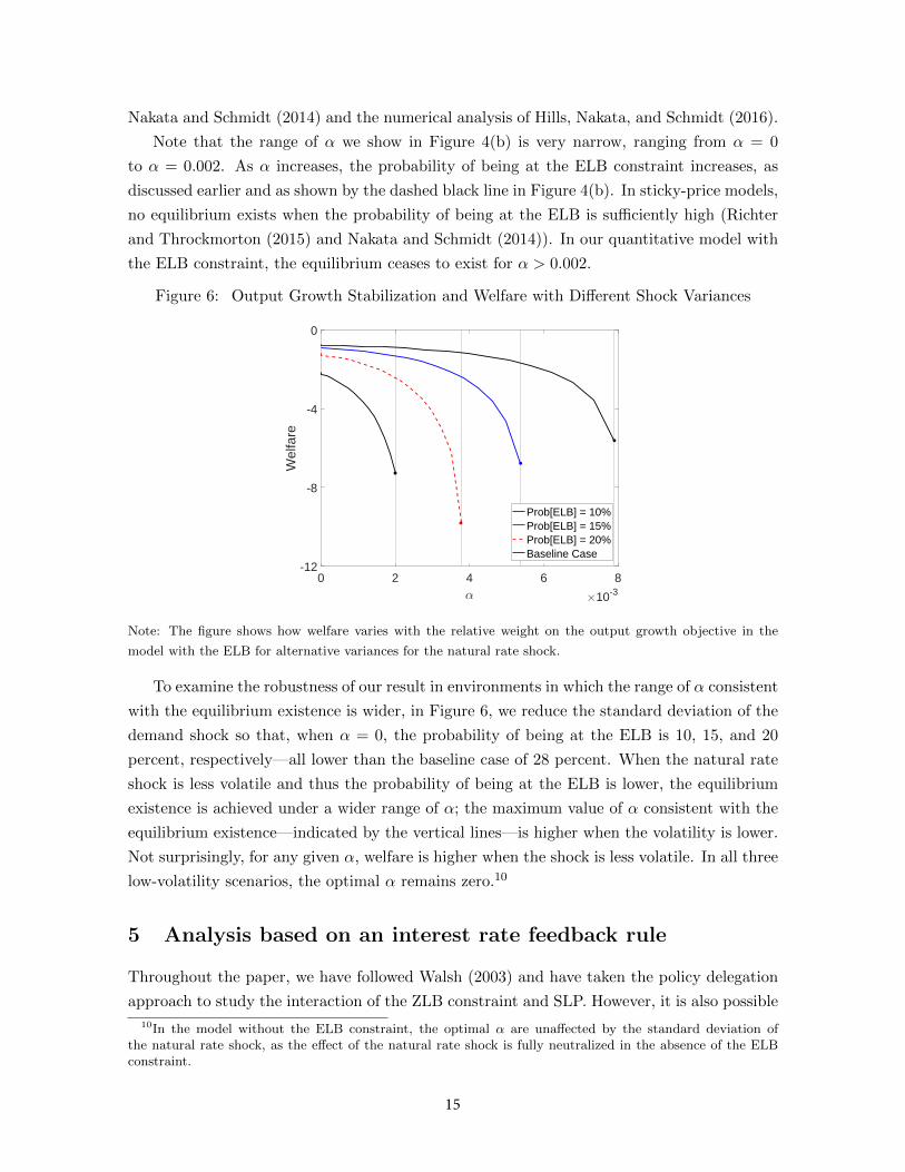
Figure 6: Output Growth Stabilization and Welfare with Different Shock Variances

0 2 4 6 8

α ×10-3

-12

-8

-4

0

Welfare

Prob[ELB] = 10%

Prob[ELB] = 15%

Prob[ELB] = 20%

Baseline Case

Note: The figure shows how welfare varies with the relative weight on the output growth objective in the

model with the ELB for alternative variances for the natural rate shock.

To examine the robustness of our result in environments in which the range of α consistent

with the equilibrium existence is wider, in Figure 6, we reduce the standard deviation of the

demand shock so that, when α = 0, the probability of being at the ELB is 10, 15, and 20

percent, respectively—all lower than the baseline case of 28 percent. When the natural rate

shock is less volatile and thus the probability of being at the ELB is lower, the equilibrium

existence is achieved under a wider range of α; the maximum value of α consistent with the

equilibrium existence—indicated by the vertical lines—is higher when the volatility is lower.

Not surprisingly, for any given α, welfare is higher when the shock is less volatile. In all three

low-volatility scenarios, the optimal α remains zero.10

5 Analysis based on an interest rate feedback rule

Throughout the paper, we have followed Walsh (2003) and have taken the policy delegation

approach to study the interaction of the ZLB constraint and SLP. However, it is also possible

10In the model without the ELB constraint, the optimal α are unaffected by the standard deviation ofthe natural rate shock, as the effect of the natural rate shock is fully neutralized in the absence of the ELBconstraint.

15

to study the interaction of the ZLB and SLP using an interest rate feedback rule with an

output growth term, as some authors have done in the past (Blake (2012); Giannoni and

Woodford (2003); Stracca (2007)).

In this section, we assume that the central bank sets the interest rate according to the

following rule and examines the desirability of SLP by varying the weight on the output

growth term. For both stylized and quantitative model, we assume that the interest rate

feedback rule is given by

it = rnt + φππt + α(yt − yt−1) (22)

in the economy without the ZLB constraint, and

it = max[iELB, i∗t ] (23)

i∗t = rnt + φππt + α(yt − yt−1) (24)

in the economy with the ELB constraint. In the following experiment, the coefficient on

inflation, φΠ, is set to 3, but all the results that ensue are robust to alternative values.

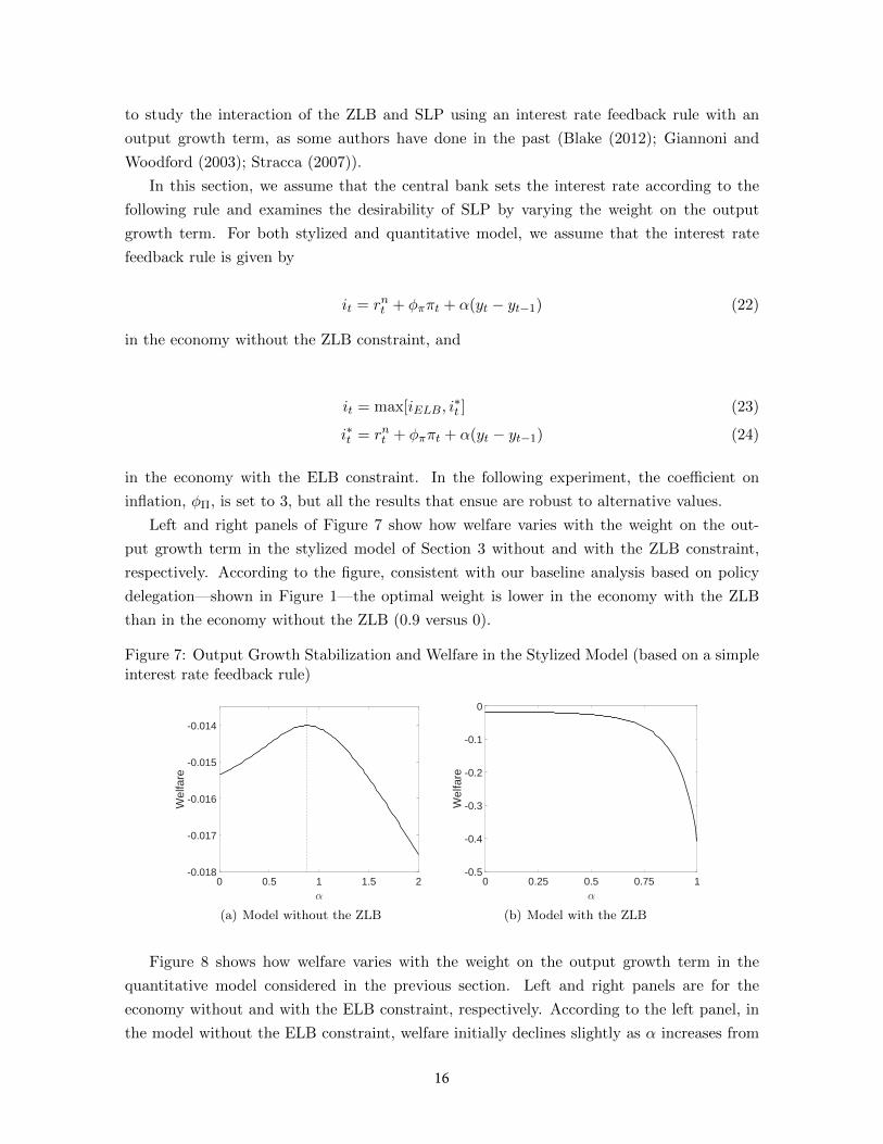
Left and right panels of Figure 7 show how welfare varies with the weight on the out-

put growth term in the stylized model of Section 3 without and with the ZLB constraint,

respectively. According to the figure, consistent with our baseline analysis based on policy

delegation—shown in Figure 1—the optimal weight is lower in the economy with the ZLB

than in the economy without the ZLB (0.9 versus 0).

Figure 7: Output Growth Stabilization and Welfare in the Stylized Model (based on a simpleinterest rate feedback rule)

0 0.5 1 1.5 2

α

-0.018

-0.017

-0.016

-0.015

-0.014

We

lfa

re

(a) Model without the ZLB

0 0.25 0.5 0.75 1

α

-0.5

-0.4

-0.3

-0.2

-0.1

0

Welfare

(b) Model with the ZLB

Figure 8 shows how welfare varies with the weight on the output growth term in the

quantitative model considered in the previous section. Left and right panels are for the

economy without and with the ELB constraint, respectively. According to the left panel, in

the model without the ELB constraint, welfare initially declines slightly as α increases from

16

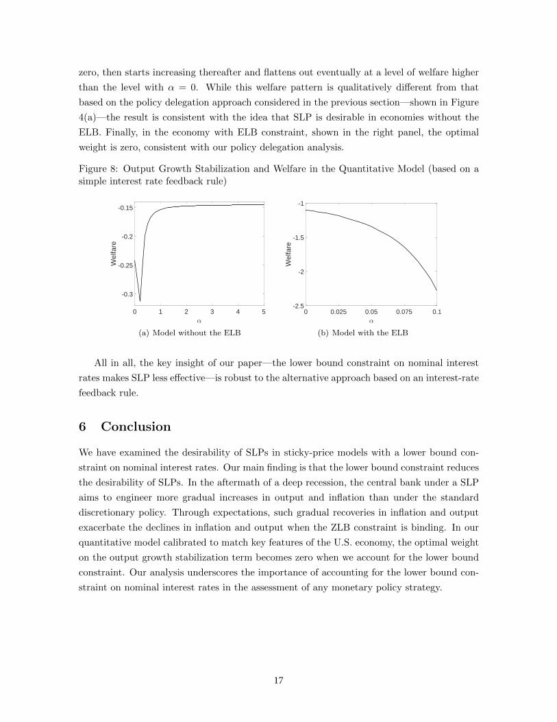
zero, then starts increasing thereafter and flattens out eventually at a level of welfare higher

than the level with α = 0. While this welfare pattern is qualitatively different from that

based on the policy delegation approach considered in the previous section—shown in Figure

4(a)—the result is consistent with the idea that SLP is desirable in economies without the

ELB. Finally, in the economy with ELB constraint, shown in the right panel, the optimal

weight is zero, consistent with our policy delegation analysis.

Figure 8: Output Growth Stabilization and Welfare in the Quantitative Model (based on asimple interest rate feedback rule)

0 1 2 3 4 5

α

-0.3

-0.25

-0.2

-0.15

We

lfa

re

(a) Model without the ELB

0 0.025 0.05 0.075 0.1

α

-2.5

-2

-1.5

-1

Welfare

(b) Model with the ELB

All in all, the key insight of our paper—the lower bound constraint on nominal interest

rates makes SLP less effective—is robust to the alternative approach based on an interest-rate

feedback rule.

6 Conclusion

We have examined the desirability of SLPs in sticky-price models with a lower bound con-

straint on nominal interest rates. Our main finding is that the lower bound constraint reduces

the desirability of SLPs. In the aftermath of a deep recession, the central bank under a SLP

aims to engineer more gradual increases in output and inflation than under the standard

discretionary policy. Through expectations, such gradual recoveries in inflation and output

exacerbate the declines in inflation and output when the ZLB constraint is binding. In our

quantitative model calibrated to match key features of the U.S. economy, the optimal weight

on the output growth stabilization term becomes zero when we account for the lower bound

constraint. Our analysis underscores the importance of accounting for the lower bound con-

straint on nominal interest rates in the assessment of any monetary policy strategy.

17

References

Bilbiie, F. O. (2014): “Delegating Optimal Monetary Policy Inertia,” Journal of Economic

Dynamics and Control, 48, 63–78.

Billi, R. M. (2013): “Nominal GDP Targeting and the Zero Lower Bound: Should We

Abandon Inflation Targeting?,” Working Paper Series 270, Sveriges Riksbank.

Blake, A. P. (2012): “Determining Optimal Monetary Speed Limits,” Economics Letters,

116(2), 269–271.

Blake, A. P., T. Kirsanova, and T. Yates (2013): “Monetary Policy Delegation and

Equilibrium Coordination,” Miemo.

Bodenstein, M., and J. Zhao (2017): “On Targeting Frameworks and Optimal Monetary

Policy,” Finance and Economics Discussion Series 2017-98, Board of Governors of the

Federal Reserve System (U.S.).

Brendon, C., M. Paustian, and T. Yates (2013): “The Pitfalls of Speed-Limit Interest

Rate Rules at the Zero Lower Bound,” Working Paper Series 473, Bank of England.

Calvo, G. A. (1983): “Staggered Prices in a Utility-Maximizing Framework,” Journal of

Monetary Economics, 12(3), 383–398.

Christiano, L. J., and J. D. M. Fisher (2000): “Algorithms for Solving Dynamic Mod-

els with Occasionally Binding Constraints,” Journal of Economic Dynamics and Control,

24(8), 1179–1232.

Eggertsson, G. B., and M. Woodford (2003): “The Zero Bound on Interest Rates and

Optimal Monetary Policy,” Brookings Papers on Economic Activity, 34(1), 139–235.

Erceg, C. J., D. W. Henderson, and A. T. Levin (2000): “Optimal monetary policy

with staggered wage and price contracts,” Journal of Monetary Economics, 46(2), 281 –

313.

Fernandez-Villaverde, J., G. Gordon, P. A. Guerron-Quintana, and J. Rubio-

Ramırez (2015): “Nonlinear Adventures at the Zero Lower Bound,” Journal of Economic

Dynamics and Control, 57, 182–204.

Gali, J. (2015): Monetary Policy, Inflation, and the Business Cycle. Princeton: Princeton

University Press.

Giannoni, M. P., and M. Woodford (2003): “How Forward-Looking is Optimal Monetary

Policy?,” Journal of Money, Credit and Banking, 35(6), 1425–1469.

18

Hills, T. S., T. Nakata, and S. Schmidt (2016): “The Risky Steady State and the

Interest Rate Lower Bound,” Finance and Economics Discussion Series 2016-9, Board of

Governors of the Federal Reserve System (U.S.).

Hirose, Y., and T. Sunakawa (2015): “Parameter Bias in an Estimated DSGE Model:

Does Nonlinearity Matter?,” Mimeo.

Maliar, L., and S. Maliar (2015): “Merging Simulation and Projection Approaches to

Solve High-Dimensional Problems with an Application to a New Keynesian Model,” Quan-

titative Economics, 6(1), 1–47.

Nakata, T., and S. Schmidt (2014): “Conservatism and Liquidity Traps,” Finance and

Economics Discussion Series 2014-105, Board of Governors of the Federal Reserve System

(U.S.).

(2016): “Gradualism and Liquidity Traps,” Finance and Economics Discussion

Series 2016-092, Board of Governors of the Federal Reserve System (U.S.).

Orphanides, A., R. D. Porter, D. Reifschneider, R. Tetlow, and F. Finan (2000):

“Errors in the Measurement of the Output Gap and the Design of Monetary Policy,”

Journal of Economics and Business, 52, 117–141.

Orphanides, A., and J. C. Williams (2002): “Robust Monetary Policy Rules with Un-

known Natural Rates,” Brookings Papers on Economic Activity, 33(2), 63–146.

(2007): “Robust Monetary Policy with Imperfect Knowledge,” Journal of Monetary

Economics, 54(5), 1406–1435.

Persson, T., and G. Tabellini (1993): “Designing Institutions for Monetary Stability,”

Carnegie-Rochester Conference Series on Public Policy, 39(1), 53–84.

Richter, A. W., and N. A. Throckmorton (2015): “The Zero Lower Bound: Frequency,

Duration, and Numerical Convergence,” B.E. Journal of Macroeconomics: Contributions,

15(1), 157–182.

Rogoff, K. (1985): “The Optimal Degree of Commitment to an Intermediate Monetary

Target,” The Quarterly Journal of Economics, 100(4), 1169–89.

Stracca, L. (2007): “A Speed Limit Monetary Policy Rule for the Euro Area,” International

Finance, 10(1), 21–41.

Svensson, L. E. O. (1997): “Optimal Inflation Targets, ‘Conservative’ Central Banks, and

Linear Inflation Contracts,” American Economic Review, 87(1), 98–114.

Walsh, C. E. (1995): “Optimal Contracts for Central Bankers,” American Economic Re-

view, 85(1), 150–67.

19

(2003): “Speed Limit Policies: The Output Gap and Optimal Monetary Policy,”

American Economic Review, 93(1), 265–278.

Williams, J. C. (2017): “Preparing for the Next Storm: Reassessing Frameworks & Strate-

gies in a Low R-Star World,” Remarks to The Shadow Open Market Committee.

Woodford, M. (2003): Interest and Prices: Foundations of a Theory of Monetary Policy.

Princeton: Princeton University Press.

20

Technical Appendix

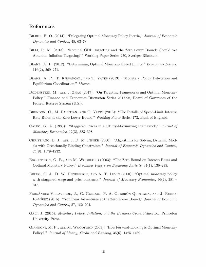
A Stylized model with AR(1) cost-push and natural rate shocks

In the main body of the paper, we have used a stylized model with a two-state Markov natural-rate shock and a three-state Markov cost-push shock to examine how the ZLB constraintaffects the desirability of speed-limit policy. In Figure 9, we conduct the same analysis in thestylized model in which the natural-rate and cost-push shocks both follow AR(1) processes.According to the figure, the optimal weight on the output growth stabilization term is lowerin the economy with the ZLB than in the economy without the ZLB, consistent with theanalysis with two-state and three-state Markov shocks.

Figure 9: Output Growth Stabilization and Welfare in the Stylize Model with AR(1) Shocks

0 1 2 3 4 5

α ×10-3

-0.065

-0.06

-0.055

-0.05

Welfare

Model without ZLB

Model with ZLB

B The Solution Method

We use a time-iteration method to solve stylized and quantitative models. In this section,we illustrate our time-iteration method using the quantitative model. It is straightforwardto apply the method to the stylized model.11

There are total of five state variables, which we denote by St 3 [ut, rnt , π

pt−1, wt−1, yt−1].

The problem is to find a set of policy functions, {πp(St), πw(St), y(St), w(St), i(St), φ1(St),11One simply needs to apply the same method to different equilibrium conditions, recognizing that there

are only three state variables (ut, rnt , and yt−1).

21

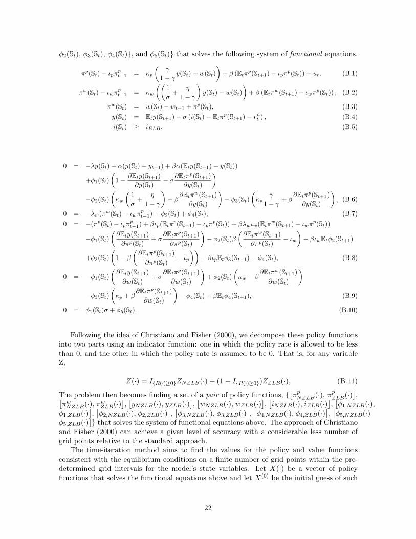
φ2(St), φ3(St), φ4(St)}, and φ5(St)} that solves the following system of functional equations.

πp(St)− ιpπpt−1 = κp

(γ

1− γy(St) + w(St)

)+ β (Etπ

p(St+1)− ιpπp(St)) + ut, (B.1)

πw(St)− ιwπpt−1 = κw

((1

σ+

η

1− γ

)y(St)− w(St)

)+ β (Etπ

w(St+1)− ιwπp(St)) , (B.2)

πw(St) = w(St)− wt−1 + πp(St), (B.3)

y(St) = Ety(St+1)− σ (i(St)− Etπp(St+1)− rnt ) , (B.4)

i(St) ≥ iELB . (B.5)

0 = −λy(St)− α(y(St)− yt−1) + βα(Ety(St+1)− y(St))

+φ1(St)(

1− ∂Ety(St+1)

∂y(St)− σ∂Etπ

p(St+1)

∂y(St)

)−φ2(St)

(κw

(1

σ+

η

1− γ

)+ β

∂Etπw(St+1)

∂y(St)

)− φ3(St)

(κp

γ

1− γ+ β

∂Etπp(St+1)

∂y(St)

), (B.6)

0 = −λw(πw(St)− ιwπpt−1) + φ2(St) + φ4(St), (B.7)

0 = −(πp(St)− ιpπpt−1) + βιp(Etπ

p(St+1)− ιpπp(St)) + βλwιw(Etπw(St+1)− ιwπp(St))

−φ1(St)(∂Ety(St+1)

∂πp(St)+ σ

∂Etπp(St+1)

∂πp(St)

)− φ2(St)β

(∂Etπ

w(St+1)

∂πp(St)− ιw

)− βιwEtφ2(St+1)

+φ3(St)(

1− β(∂Etπ

p(St+1)

∂πp(St)− ιp

))− βιpEtφ3(St+1)− φ4(St), (B.8)

0 = −φ1(St)(∂Ety(St+1)

∂w(St)+ σ

∂Etπp(St+1)

∂w(St)

)+ φ2(St)

(κw − β

∂Etπw(St+1)

∂w(St)

)−φ3(St)

(κp + β

∂Etπp(St+1)

∂w(St)

)− φ4(St) + βEtφ4(St+1), (B.9)

0 = φ1(St)σ + φ5(St). (B.10)

Following the idea of Christiano and Fisher (2000), we decompose these policy functionsinto two parts using an indicator function: one in which the policy rate is allowed to be lessthan 0, and the other in which the policy rate is assumed to be 0. That is, for any variableZ,

Z(·) = I{R(·)≥0}ZNZLB(·) + (1− I{R(·)≥0})ZZLB(·), (B.11)

The problem then becomes finding a set of a pair of policy functions, {[πpNZLB(·), πpZLB(·)

],[

πwNZLB(·), πwZLB(·)],[yNZLB(·), yZLB(·)

],[wNZLB(·), wZLB(·)

],[iNZLB(·), iZLB(·)

],[φ1,NZLB(·),

φ1,ZLB(·)],[φ2,NZLB(·), φ2,ZLB(·)

],[φ3,NZLB(·), φ3,ZLB(·)

],[φ4,NZLB(·), φ4,ZLB(·)

],[φ5,NZLB(·)

φ5,ZLB(·)]} that solves the system of functional equations above. The approach of Christiano

and Fisher (2000) can achieve a given level of accuracy with a considerable less number ofgrid points relative to the standard approach.

The time-iteration method aims to find the values for the policy and value functionsconsistent with the equilibrium conditions on a finite number of grid points within the pre-determined grid intervals for the model’s state variables. Let X(·) be a vector of policyfunctions that solves the functional equations above and let X(0) be the initial guess of such

22

policy functions.12 At the s-th iteration, given the approximated policy function X(s−1)(·),we solve the system of nonlinear equations given by equations (B.1)-(B.10) to find today’sπpt , π

wt , yt, wt, it, φ1,t, φ2,t, φ3,t, φ4,t, and φ5,t at each grid point. In solving the system of

nonlinear equations, we use Gaussian quadrature (with 10 Gauss-Hermite nodes) to discretizeand evaluate the expectation terms in the Euler equation, the price and wage Phillips curves,and expectational partial derivative terms.

The values of the policy function that are not on any of the grid points are interpolatedor extrapolated linearly. The values of the partial derivatives of the policy functions not onany of the grid points are approximated by the slope of the policy functions evaluated fromthe adjacent two grid points. That is, for any variable X and Z,

∂X(δt+1,t )

∂Zt=X(δt+1, Z

′′)−X(δt+1, Z

′)

Z ′′ − Z ′. (B.12)

where Z′

and Z′′

are two adjacent grid points to Zt such that Z′< Zt < Z

′′. When Zt is

outside the grid interval, the partial derivative is approximated by the slope evaluated at theedge of the grid interval.

The system is solved numerically by using a nonlinear equation solver, dneqnf, providedby the IMSL Fortran Numerical Library. If the updated policy functions are sufficientlyclose to the previously approximated policy functions, then the iteration ends. Otherwise,using the former as the guess for the next period’s policy functions, we iterate on this pro-cess until the difference between the guessed and updated policy functions is sufficientlysmall (

∥∥vec(Xs(δ)−Xs−1(δ))∥∥∞ < 1e-12 is used as the convergence criteria). The solution

method can be extended to models with multiple (non-perfectly correlated) exogenous shocksand with multiple endogenous state variables in a straightforward way.

C Solution Accuracy

In this section, we report the accuracy of our numerical solutions for the stylized and empiricalmodels. Following Fernandez-Villaverde, Gordon, Guerron-Quintana, and Rubio-Ramırez(2015) and Maliar and Maliar (2015), we evaluate these residuals functions along a simulatedequilibrium path. The length of the simulation is 100,000.

C.1 Stylized model

For the stylized model, there are three key residual functions of interest. The first two residualfunctions, denoted by R1,t and R2,t, are associated with the sticky-price equation and theEuler equation, respectively (equations (1) and (2)). The last residual function, denoted byR3,t, is associated with the first-order conditions of the central bank’s optimization problemwith respect to price inflation. For each equation, the residual function is defined as theabsolute value of the difference between the left-hand side and the right-hand side of theequation. Table 3 shows the average and the 95th percentile of the six residual functionsover the 100,000 simulations. The size of the residuals are comparable to those reportedin other numerical works on the New Keynesian model with the ELB constraint, such asFernandez-Villaverde, Gordon, Guerron-Quintana, and Rubio-Ramırez (2015), Hills, Nakata,and Schmidt (2016), Hirose and Sunakawa (2015), and Maliar and Maliar (2015).

12For all models and all variables, we use flat functions at the deterministic steady-state values as the initialguess.

23

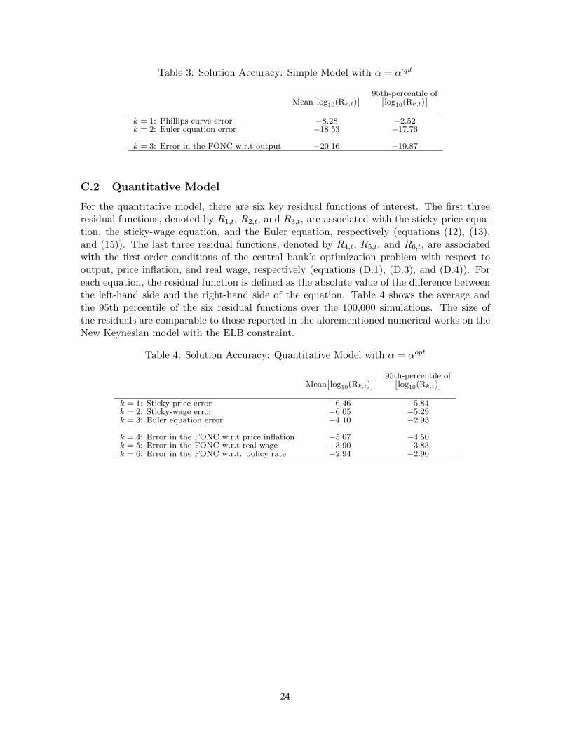
Table 3: Solution Accuracy: Simple Model with α = αopt

95th-percentile ofMean

[log10(Rk,t)

] [log10(Rk,t)

]k = 1: Phillips curve error −8.28 −2.52k = 2: Euler equation error −18.53 −17.76

k = 3: Error in the FONC w.r.t output −20.16 −19.87

C.2 Quantitative Model

For the quantitative model, there are six key residual functions of interest. The first threeresidual functions, denoted by R1,t, R2,t, and R3,t, are associated with the sticky-price equa-tion, the sticky-wage equation, and the Euler equation, respectively (equations (12), (13),and (15)). The last three residual functions, denoted by R4,t, R5,t, and R6,t, are associatedwith the first-order conditions of the central bank’s optimization problem with respect tooutput, price inflation, and real wage, respectively (equations (D.1), (D.3), and (D.4)). Foreach equation, the residual function is defined as the absolute value of the difference betweenthe left-hand side and the right-hand side of the equation. Table 4 shows the average andthe 95th percentile of the six residual functions over the 100,000 simulations. The size ofthe residuals are comparable to those reported in the aforementioned numerical works on theNew Keynesian model with the ELB constraint.

Table 4: Solution Accuracy: Quantitative Model with α = αopt

95th-percentile ofMean

[log10(Rk,t)

] [log10(Rk,t)

]k = 1: Sticky-price error −6.46 −5.84k = 2: Sticky-wage error −6.05 −5.29k = 3: Euler equation error −4.10 −2.93

k = 4: Error in the FONC w.r.t price inflation −5.07 −4.50k = 5: Error in the FONC w.r.t real wage −3.90 −3.83k = 6: Error in the FONC w.r.t. policy rate −2.94 −2.90

24

D First-Order Necessary Conditions for Central Bank’s Prob-lem in the Quantitative Model

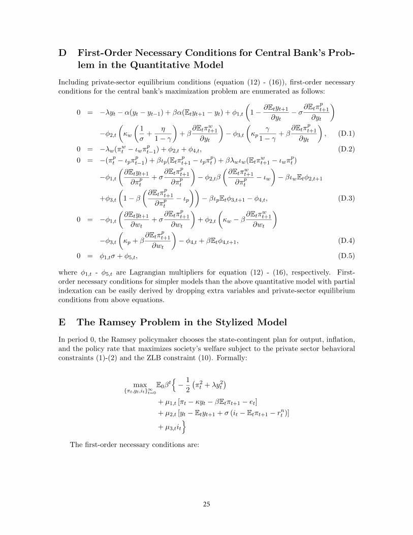
Including private-sector equilibrium conditions (equation (12) - (16)), first-order necessaryconditions for the central bank’s maximization problem are enumerated as follows:

0 = −λyt − α(yt − yt−1) + βα(Etyt+1 − yt) + φ1,t

(1− ∂Etyt+1

∂yt− σ

∂Etπpt+1

∂yt

)−φ2,t

(κw

(1

σ+

η

1− γ

)+ β

∂Etπwt+1

∂yt

)− φ3,t

(κp

γ

1− γ+ β

∂Etπpt+1

∂yt

), (D.1)

0 = −λw(πwt − ιwπpt−1) + φ2,t + φ4,t, (D.2)

0 = −(πpt − ιpπpt−1) + βιp(Etπpt+1 − ιpπ

pt ) + βλwιw(Etπwt+1 − ιwπ

pt )

−φ1,t

(∂Etyt+1

∂πpt+ σ

∂Etπpt+1

∂πpt

)− φ2,tβ

(∂Etπwt+1

∂πpt− ιw

)− βιwEtφ2,t+1

+φ3,t

(1− β

(∂Etπpt+1

∂πpt− ιp

))− βιpEtφ3,t+1 − φ4,t, (D.3)

0 = −φ1,t

(∂Etyt+1

∂wt+ σ

∂Etπpt+1

∂wt

)+ φ2,t

(κw − β

∂Etπwt+1

∂wt

)−φ3,t

(κp + β

∂Etπpt+1

∂wt

)− φ4,t + βEtφ4,t+1, (D.4)

0 = φ1,tσ + φ5,t, (D.5)

where φ1,t - φ5,t are Lagrangian multipliers for equation (12) - (16), respectively. First-order necessary conditions for simpler models than the above quantitative model with partialindexation can be easily derived by dropping extra variables and private-sector equilibriumconditions from above equations.

E The Ramsey Problem in the Stylized Model

In period 0, the Ramsey policymaker chooses the state-contingent plan for output, inflation,and the policy rate that maximizes society’s welfare subject to the private sector behavioralconstraints (1)-(2) and the ZLB constraint (10). Formally:

max{πt,yt,it}∞t=0

E0βt{− 1

2

(π2t + λy2

t

)+ µ1,t [πt − κyt − βEtπt+1 − et]+ µ2,t [yt − Etyt+1 + σ (it − Etπt+1 − rnt )]

+ µ3,tit

}The first-order necessary conditions are:

25

0 = πt − µ1,t + µ1,t−1 +σ

βµ2,t−1 (E.1)

0 = λyt + κµ1,t − µ2,t +1

βµ2,t−1 (E.2)

0 = σµ2,t + µ3,t (E.3)

µ3,t ≥ 0, it ≥ 0 (E.4)

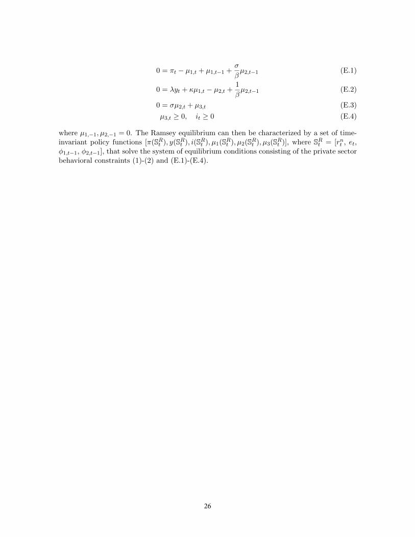
where µ1,−1, µ2,−1 = 0. The Ramsey equilibrium can then be characterized by a set of time-invariant policy functions [π(SRt ), y(SRt ), i(SRt ), µ1(SRt ), µ2(SRt ), µ3(SRt )], where SRt = [rnt , et,φ1,t−1, φ2,t−1], that solve the system of equilibrium conditions consisting of the private sectorbehavioral constraints (1)-(2) and (E.1)-(E.4).

26