Embed Size (px)
Citation preview

1
Innovations Required in Data Reconstruction
Jeffrey A. Fessler
EECS DepartmentUniversity of Michigan
Summit on Management of Radiation Dose in Computerized Tomography:Toward the Sub-mSv Exam
Feb. 15, 2011
http://www.eecs.umich.edu/∼fessler

2
Full disclosure
• Research support from GE Healthcare• Research support to GE Global Research• Work supported in part by NIH grant R01-HL-098686• Research support from Intel
3
Credits
Current students / post-docs
• Jang Hwan Cho
• Wonseok Huh
• Donghwan Kim
• Yong Long
• Madison McGaffin
• Sathish Ramani
• Stephen Schmitt
• Meng Wu
GE collaborators
• Jiang Hsieh
• Jean-Baptiste Thibault
• Bruno De Man
CT collaborators
• Mitch Goodsitt, UM
• Ella Kazerooni, UM
• Neal Clinthorne, UM
• Paul Kinahan, UW
Former PhD students (who did/do CT)
• Se Young Chun, Harvard / Brigham
• Hugo Shi, Enthought
• Joonki Noh, Emory
• Somesh Srivastava, JHU
• Rongping Zeng, FDA
• Yingying, Zhang-O’Connor, RGM Advisors
• Matthew Jacobson, Xoran
• Sangtae Ahn, GE
• Idris Elbakri, CancerCare / Univ. of Manitoba
• Saowapak Sotthivirat, NSTDA Thailand
• Web Stayman, JHU
• Feng Yu, Univ. Bristol
• Mehmet Yavuz, Qualcomm
• Hakan Erdogan, Sabanci University
Former MS students
• Kevin Brown, Philips
• ...
4
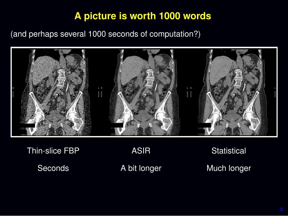
A picture is worth 1000 words
(and perhaps several 1000 seconds of computation?)
Thin-slice FBP ASIR Statistical
Seconds A bit longer Much longer

5
Why statistical methods for CT?
• Accurate physical models◦ X-ray spectrum, beam-hardening, scatter, ...
reduced artifacts? quantitative CT?◦ X-ray detector spatial response, focal spot size, ...
improved spatial resolution?◦ detector spectral response (e.g., photon-counting detectors)
• Nonstandard geometries◦ transaxial truncation (big patients)◦ long-object problem in helical CT◦ irregular sampling in “next-generation” geometries◦ coarse angular sampling in image-guidance applications◦ limited angular range (tomosynthesis)◦ “missing” data, e.g., bad pixels in flat-panel systems
• Appropriate statistical models◦ weighting reduces influence of photon-starved rays
(FBP treats all rays equally)◦ reducing image noise or dose

6
and more...
• Object constraints◦ nonnegativity◦ object support◦ piecewise smoothness◦ object sparsity (e.g., angiography)◦ sparsity in some basis◦ motion models◦ dynamic models◦ ...
Disadvantages?• Computation time (super computer)• Must reconstruct entire FOV• Model complexity• Software complexity• Algorithm nonlinearities◦ Difficult to analyze resolution/noise properties (cf. FBP)◦ Tuning parameters◦ Challenging to characterize performance
7
Flavors of “Statistical” reconstruction
• Image domain• Sinogram domain• Fully statistical (both)• Hybrid methods

8
“Statistical” methods: Image domain
• Denoising methods
sinogramyyy
→ FBP →noisy
reconstructionxxx
→iterativedenoiser
→final
imagexxx
◦ Relatively fast, even if iterative◦ Remarkable advances in denoising methods in last decade
Zhu & Milanfar, T-IP, Dec. 2010, using “steering kernel regression” (SKR) method
Challenges:◦ Typically assume white noise◦ Streaks in low-dose FBP appear like edges (highly correlated noise)

• Image denoising methods “guided by data statistics”
sinogramyyy
→ FBP →noisy
reconstructionxxx
→magicaliterativedenoiser
↑sinogramstatistics?
→final
imagexxx
◦ Image-domain methods are fast (thus practical)◦ ASIR? IRIS? ...◦ The technical details are a mystery...
Challenges:◦ FBP often does not use all data efficiently (e.g., Parker weighting)◦ Low-dose CT statistics most naturally expressed in sinogram domain

10
“Statistical” methods: Sinogram domain
• Sinogram restoration methods
noisysinogram
yyy
→adaptive
or iterativedenoiser
→cleaned
sinogramyyy
→ FBP →final
imagexxx
◦ Adaptive: J. Hsieh, Med. Phys., 1998; Kachelrieß, Med. Phys., 2001, ...
◦ Iterative: P. La Riviere, IEEE T-MI, 2000, 2005, 2006, 2008
◦ Relatively fast even if iterativeChallenges:◦ Limited denoising without resolution loss◦ Difficult to “preserve edges” in sinograms
FBP, 10 mA FBP from denoised sinogramWang et al., T-MI, Oct. 2006, using PWLS-GS on sinogram

11
(True? Fully? Slow?) Statistical reconstruction
• Object model• Physics/system model• Statistical model• Cost function (log-likelihood + regularization)• Iterative algorithm for minimization
“Find the image xxx that best fits the sinogram data yyy according to the physicsmodel, the statistical model and prior information about the object”
ModelSystem
Iteration
Parameters
MeasurementsProjection
Calibration ...
Ψxxx(n) xxx(n+1)
• Repeatedly revisiting the sinogram data can use statistics fully
• Repeatedly updating the image can exploit object properties
• ... greatest potential dose reduction, but repetition is expensive...

12
History: Statistical reconstruction for PET
• Iterative method for emission tomography (Kuhl, 1963)
• Weighted least squares for 3D SPECT (Goitein, NIM, 1972)
• Richardson/Lucy iteration for image restoration (1972, 1974)
• Poisson likelihood (emission) (Rockmore and Macovski, TNS, 1976)
• Expectation-maximization (EM) algorithm (Shepp and Vardi, TMI, 1982)
• Regularized (aka Bayesian) Poisson emission reconstruction(Geman and McClure, ASA, 1985)
• Ordered-subsets EM (OSEM) algorithm (Hudson and Larkin, TMI, 1994)
• Commercial release of OSEM for PET scanners circa 1997
Key factors• OS algorithm accelerated convergence by order of magnitude• Computers got faster (but problem size grew too)• Key clinical validation papers?• Nuclear medicine physicians grew accustomed to appearance of images
reconstructed using statistical methods

13
Five Choices for Statistical Reconstruction
1. Object model
2. System physical model
3. Measurement statistical model
4. Cost function: data-mismatch and regularization
5. Algorithm / initialization
There are challenges with each choice.

14
Choice 1. Object Parameterization
Finite measurements: {yi}Mi=1. Continuous object: f (~r) = µ(~r).
“All models are wrong but some models are useful.”
Linear series expansion approach. Represent f (~r) by xxx = (x1, . . . ,xN) where
f (~r)≈ f (~r) =N
∑j=1
x j b j(~r) ← “basis functions”
Reconstruction problem becomes “discrete-discrete:” estimate xxx from yyy
Challenges• Compact (voxels) versus band-limited (but bigger) blobs• Choice of voxel size (resolution vs computation)• Must cover entire object
One practical compromise: wide FOV coarse-grid reconstruction followedby fine-grid refinement over ROI, e.g., Ziegler et al., Med. Phys., Apr. 2008

15
Global reconstruction: An inconvenient truth
70-cm FOV reconstruction
Thibault et al., Fully3D, 2007
16
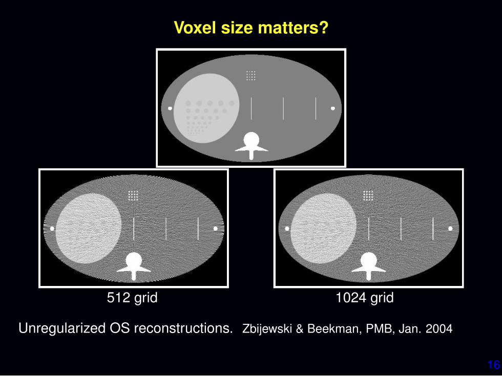
Voxel size matters?
512 grid 1024 grid
Unregularized OS reconstructions. Zbijewski & Beekman, PMB, Jan. 2004

17
Choice 2. System model / Physics model
• scan geometry• source intensity I0
◦ spatial variations (air scan)◦ intensity fluctuations
• resolution effects◦ finite detector size / detector spatial response◦ finite X-ray spot size / anode angulation Inhomogeneous◦ detector afterglow
• spectral effects◦ X-ray source spectrum◦ bowtie filters◦ detector spectra response
• scatter• ...
Challenges• computation time versus accuracy/artifacts/resolution/contrast• dose?

18
Lines versus strips
From (De Man and Basu, PMB, Jun. 2004) MLTR of rabbit heart
Ray-driven (idealized point detector)
Distance-driven (models finite detector width)

19
Projector/back-projector bottleneck
Challenges
• Projector/backprojector algorithm design◦ Approximations (e.g., transaxial/axial separability)◦ Symmetry
• Hardware / software implementation◦ GPU, CUDA, OpenCL, FPGA, SIMD, pthread, OpenMP, MPI, ...
• Further “wholistic” approaches?e.g., Basu & De Man, “Branchless distance driven projection ...,” SPIE 2006
• ...
20
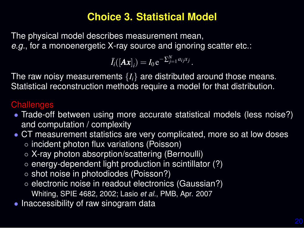
Choice 3. Statistical Model
The physical model describes measurement mean,e.g., for a monoenergetic X-ray source and ignoring scatter etc.:
Ii([AAAxxx]i) = I0 e−∑N
j=1 ai jx j .
The raw noisy measurements {Ii} are distributed around those means.Statistical reconstruction methods require a model for that distribution.
Challenges• Trade-off between using more accurate statistical models (less noise?)
and computation / complexity• CT measurement statistics are very complicated, more so at low doses◦ incident photon flux variations (Poisson)◦ X-ray photon absorption/scattering (Bernoulli)◦ energy-dependent light production in scintillator (?)◦ shot noise in photodiodes (Poisson?)◦ electronic noise in readout electronics (Gaussian?)
Whiting, SPIE 4682, 2002; Lasio et al., PMB, Apr. 2007
• Inaccessibility of raw sinogram data

21
To log() or not to log() – That is the question
Models for “raw” data Ii (before logarithm)
• compound Poisson (complicated) Whiting, SPIE 4682, 2002;
Elbakri & Fessler, SPIE 5032, 2003; Lasio et al., PMB, Apr. 2007
• Poisson + Gaussian (photon variability and electronic readout noise):
Ii ∼ Poisson{Ii}+N(
0,σ2)
Snyder et al., JOSAA, May 1993 & Feb. 1995
• Shifted Poisson approximation (matches first two moments):
Ii ,[
Ii +σ2]
+∼ Poisson
{
Ii +σ2}
Yavuz & Fessler, MIA, Dec. 1998
• Ordinary Poisson (ignore electronic noise):
Ii ∼ Poisson{Ii}
Rockmore and Macovski, TNS, Jun. 1977; Lange and Carson, JCAT, Apr. 1984
• Photon-counting detectors would simplify statistical modeling
All are somewhat complicated by the nonlinearity of the physics: Ii = e−[AAAxxx]i

22
After taking the log()
Taking the log leads to a linear model (ignoring beam hardening):
yi ,− log
(
Ii
I0
)
≈ [AAAxxx]i + εi
Drawbacks:• Undefined if Ii ≤ 0 (e.g., due to electronic noise)• It is biased (by Jensen’s inequality): E[yi]≥− log(Ii/I0) = [AAAxxx]i• Exact distribution of noise εi intractable
Practical approach: assume Gaussian noise model: εi ∼ N(
0,σ2i
)
Options for modeling noise variance σ2i = Var{εi}
• consider both Poisson and Gaussian noise effects: σ2i = Ii+σ2
I2i
Thibault et al., SPIE 6065, 2006
• consider just Poisson effect: σ2i = 1
Ii(Sauer & Bouman, T-SP, Feb. 1993)
• pretend it is white noise: σ2i = σ2
0
• ignore noise altogether and “solve” yyy = AAAxxx
Whether using pre-log data is better than post-log data is an open question.

23
Choice 4. Cost Functions
Components:• Data-mismatch term• Regularization term (and regularization parameter β)• Constraints (e.g., nonnegativity)
Reconstruct image xxx by minimizing a cost function:
xxx , argminxxx≥000
Ψ(xxx)
Ψ(xxx) = DataMismatch(yyy,AAAxxx)+βRegularizer(xxx)
Forcing too much “data fit” alone would give noisy images.
Equivalent to a Bayesian MAP (maximum a posteriori) estimator.
Distinguishes “statistical methods” from “algebraic methods” for “yyy = AAAxxx.”

24
Choice 4.1: Data-Mismatch Term
Standard choice is the negative log-likelihood of statistical model:
DataMismatch =−L(xxx;yyy) =− logp(yyy|xxx) =M
∑i=1
− logp(yi|xxx) .
• For pre-log data III with shifted Poisson model:
−L(xxx; III) =M
∑i=1
(
Ii +σ2)
−[
Ii +σ2]
+log
(
Ii +σ2)
, Ii = I0 e−[AAAxxx]i
This can be non-convex if σ2 > 0;it is convex if we ignore electronic noise σ2 = 0. Trade-off ...
• For post-log data yyy with Gaussian model:
−L(xxx;yyy) =M
∑i=1
wi
1
2(yi− [AAAxxx]i)
2 =1
2(yyy−AAAxxx)′WWW (yyy−AAAxxx), wi = 1/σ2
i
This is a kind of (data-based) weighted least squares (WLS).It is always convex in xxx. Quadratic functions are “easy” to minimize.
• ...

25
Choice 4.2: Regularization
Controlling noise due to ill-conditioning via imposing constraints
Options for regularizer R(xxx) in increasing complexity:• quadratic roughness• convex, non-quadratic roughness• non-convex roughness• total variation• convex sparsity• non-convex sparsity
Challenges• Reducing noise without degrading spatial resolution• Balancing regularization strength between and within slices• Parameter selection• Computational complexity (voxels have 26 neighbors in 3D)• Preserving “familiar” noise texture• Optimizing clinical task performance
Many open questions...

26
Roughness Penalty Functions
R(xxx) =N
∑j=1
1
2∑
k∈N j
ψ(x j− xk)
N j , neighborhood of jth pixel (e.g., left, right, up, down)ψ called the potential function
−2 −1 0 1 20
0.5
1
1.5
2
2.5
3
Quadratic vs Non−quadratic Potential Functions
Parabola (quadratic)
Huber, δ=1
Hyperbola, δ=1
t = x j− xk
ψ(t
)
quadratic: ψ(t) = t2
hyperbola: ψ(t) =√
1+(t/δ)2
(edge preservation)

27
Regularization parameters: Dramatic effects
Thibault et al., Med. Phys., Nov. 2007
“q generalized gaussian” potential function with tuning parameters: β,δ, p,q:
βψ(t) = β
12|t|p
1+ |t/δ|p−q
p = q = 2 p = 2, q = 1.2, δ = 10 HU p = q = 1.1
noise: 11.1 10.9 10.8(#lp/cm): 4.2 7.2 8.2

28
Summary thus far
1. Object parameterization
2. System physical model
3. Measurement statistical model
4. Cost function: data-mismatch / regularization / constraints
Reconstruction Method , Models + Cost Function + Algorithm
5. Minimization algorithms:
xxx = argminxxx
Ψ(xxx)

29
Choice 5: Minimization algorithms
• Conjugate gradients◦ Converges slowly for CT◦ Difficult to precondition due to weighting and regularization◦ Difficult to enforce nonnegativity constraint◦ Very easily parallelized
• Ordered subsets◦ Initially converges faster than CG if many subsets used◦ Does not converge without relaxation etc., but those slow it down◦ Computes regularizer gradient ∇R(xxx) for every subset - expensive?◦ Easily enforces nonnegativity constraint◦ Easily parallelized
• Coordinate descent (Sauer and Bouman, T-SP, 1993)
◦ Converges high spatial frequencies rapidly, but low frequencies slowly◦ Easily enforces nonnegativity constraint◦ Challenging to parallelize
• Block coordinate descent (Benson et al., NSS/MIC, 2010)
◦ Spatial frequency convergence properties depend...◦ Easily enforces nonnegativity constraint◦ More opportunity to parallelize than CD

30
Convergence rates
(De Man et al., NSS/MIC 2005)
In terms of iterations: CD < OS < CG < Convergent OSIn terms of compute time? (it depends...)

31
Ordered subsets convergence
Theoretically OS does not converge, but it may get “close enough,” evenwith regularization.
CD200 iter
OS41 subsets
200 iter
difference0 ± 10HU
display: 930 HU ± 58 HU
(De Man et al., NSS/MIC 2005)
Ongoing saga... (SPIE, ISBI, Fully 3D, ...)
32
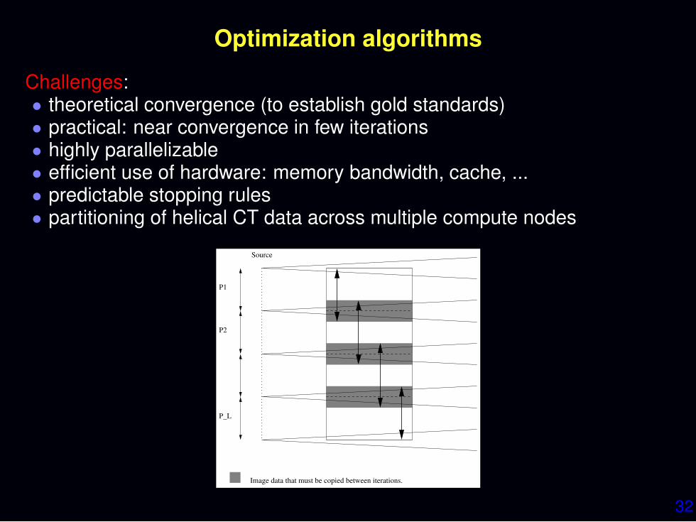
Optimization algorithms
Challenges:• theoretical convergence (to establish gold standards)• practical: near convergence in few iterations• highly parallelizable• efficient use of hardware: memory bandwidth, cache, ...• predictable stopping rules• partitioning of helical CT data across multiple compute nodes
P1
P2
P_L
Source
Image data that must be copied between iterations.
33
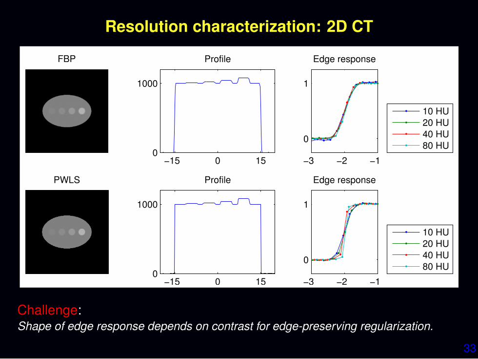
Resolution characterization: 2D CT
FBP
PWLS
−15 0 150
1000
Profile
−15 0 150
1000
Profile
−3 −2 −1
0
1
Edge response
10 HU
20 HU
40 HU
80 HU
−3 −2 −1
0
1
Edge response
10 HU
20 HU
40 HU
80 HU
Challenge:Shape of edge response depends on contrast for edge-preserving regularization.

34
Assessing image quality
Challenges:• Resolution (PSF, edge response, MTF)• Noise• Task-based performance measures
Known-location versus unknown-location tasks• ...
“How low can the dose go” – quite challenging to answer

35
Some open problems
• Modeling◦ Statistical modeling for very low-dose CT◦ Resolution effects◦ Spectral CT◦ Object motion
• Parameter selection / performance characterization◦ Performance prediction for nonquadratic regularization◦ Effect of nonquadratic regularization on detection tasks◦ Choice of regularization parameters for nonquadratic regularization
• Algorithms◦ optimization algorithm design◦ software/hardware implementation◦ Moore’s law alone will not suffice
(dual energy, dual source, motion, dynamic, smaller voxels ...)• Clinical evaluation• ...

36
The CT reconstruction research environment
Challenges• raw sinogram access is very limited (cf. PET, MRI)• CT preprocessing steps are considered highly proprietary• No standard databases of sinogram test data sets (cf. post-processing)• Trainees perceived to be data processors, not CT scientists (cf. MRI)• Commercial solutions largely will have predetermined parameters
Nevertheless, the CT reconstruction revolution will occur, like in PET...
Dr. Thrall: statistical image reconstruction will have the single largest bangfor impacting dose.