Informe no. 673 (Gas Natural): LNG Tank at Taranto (Italy

Ingenieros Consultores

14˚

14˚

16˚

16˚

18˚

18˚

20˚

20˚

38˚ 38˚

40˚ 40˚

42˚ 42˚

44˚ 44˚

Taranto

R = 320 km

LNG PLANT AT TARANTO (ITALY)

SEISMIC HAZARD EVALUATION

Report

to

Gas Natural

Report no. 673 Rev. 1 Project no. P-373

06/05/05

LNG PLANT AT TARANTO (ITALY)

SEISMIC HAZARD EVALUATION

Report

to

Gas Natural

Document ID: P373-INF-673 Revision: 1 Date: 06/05/05

Prepared: Revised: Approved: J. Rodríguez J. Martí F. Martínez

Report no. 673 Rev. 1 P-373 PRINCIPIA

inf22645.doc i

TABLE OF CONTENTS

Page

1. INTRODUCTION.............................................................................................. 1 1.1 Preamble ........................................................................................................ 1 1.2 Object ............................................................................................................ 1 1.3 Scope ............................................................................................................. 2 1.4 Layout of report............................................................................................. 3

2. DESCRIPTION OF THE PROBLEM ............................................................... 5 2.1 Relevant norms.............................................................................................. 5 2.2 General approach........................................................................................... 5 2.3 Seismic information....................................................................................... 7 2.4 Tectonic information ..................................................................................... 8 2.5 Geotechnical site information ....................................................................... 9 2.6 Attenuation laws.......................................................................................... 10 2.7 Other correlations used................................................................................ 11

3. EVALUATION OF THE HAZARD ............................................................... 21 3.1 Description of the methodology.................................................................. 21 3.2 Specification of the kernel function ............................................................ 22 3.3 Effective detection periods.......................................................................... 23 3.4 Seismic hazard at the site ............................................................................ 25

4. DESIGN MOTIONS ........................................................................................ 31 4.1 Design accelerations.................................................................................... 31 4.2 Site specific response spectra ...................................................................... 31 4.3 Matching accelerograms.............................................................................. 33

5. LOCAL SOIL RESPONSE.............................................................................. 48 5.1 Idealised cross-section................................................................................. 48 5.2 Dynamic response of the ground................................................................. 49 5.3 Evaluation of the liquefaction potential ...................................................... 50

6. CONCLUSIONS .............................................................................................. 64


inf22645.doc ii

Appendix I. References ........................................................................................ 66 Appendix II. The computer program KERFRACT.............................................. 70


inf22645.doc iii

LIST OF FIGURES

Page

Figure 2–1 Active stress map and locations of significant recent earthquakes....12 Figure 2–2 Main trends of identified seismogenetic sources...............................13 Figure 2–3 Local tectonic scheme in Taranto ......................................................14 Figure 2–4 Epicentres from the catalogue............................................................15 Figure 2–5 Epicentres with magnitudes greater than 4.0 .....................................16 Figure 2–6 SPT data for tanks and plant area ......................................................17 Figure 2–7 Wave velocities in borehole BH1 ......................................................18 Figure 2–8 Wave velocities in borehole BH5 ......................................................19 Figure 2–9 Attenuation law by Sabetta and Pugliese (1987 and 1996) ...............20 Figure 3–1 Curve-fits for bandwidth....................................................................26 Figure 3–2 Time distribution of magnitudes from year 1000 ..............................27 Figure 3–3 Time distribution of magnitudes from year 1980 ..............................28 Figure 3–4 Spectral acceleration, T = 0 s .............................................................29 Figure 3–5 Sensitivity to the power-law exponent...............................................30 Figure 4–1 Design accelerations ..........................................................................36 Figure 4–2 Hazard map proposed by the Servizio Sismico Nazionale................37 Figure 4–3 Horizontal design spectra...................................................................38 Figure 4–4 Vertical design spectra .......................................................................39 Figure 4–5 SSE horizontal accelerograms ...........................................................40 Figure 4–6 SSE vertical accelerograms................................................................41 Figure 4–7 OBE horizontal accelerograms ..........................................................42 Figure 4–8 OBE vertical accelerograms ..............................................................43 Figure 4–9 Matching spectra for the horizontal SSE ...........................................44 Figure 4–10 Matching spectra for the vertical SSE .............................................45 Figure 4–11 Matching spectra for the horizontal OBE........................................46 Figure 4–12 Matching spectra for the vertical OBE ............................................47 Figure 5–1 Damping and normalised G modulus vs effective strain...................54 Figure 5–2 Liquefaction resistance for sands - SPT ............................................55 Figure 5–3 Liquefaction resistance for sands - CPT ............................................56 Figure 5–4 Corrected values (N1)60 ......................................................................57 Figure 5–5 CPT – Cone penetration resistance....................................................58 Figure 5–6 CPT – Sleeve resistance.....................................................................59 Figure 5–7 CRR for layers 1 and 4.......................................................................60


inf22645.doc iv

Figure 5–8 Seismic demand in terms of CSR ......................................................61 Figure 5–9 Comparison of demand (CSR) and resistance (CRR) .......................62 Figure 5–10 (N1)60 values under Tank 1 compared with requirement .................63


inf22645.doc v

LIST OF TABLES

Page

Table 3–1 Reference years for different event intensities....................................24 Table 5–1 Dynamic properties .............................................................................48 Table 5–2 OBE. Equivalent dynamic properties..................................................49 Table 5–3 SSE. Equivalent dynamic properties...................................................50 Table 5–4 Lower, average and upper values of (N1)60 .........................................51 Table 5–5 Lower, average and upper values of CRR ..........................................52 Table 5–6 Percentile fractions of (N1)60 data below 22........................................53


inf22645.doc 1

1. INTRODUCTION

1.1 Preamble

Gas Natural is planning to construct an import and regasification plant for liquefied natural gas (LNG) at Taranto (Italy), which includes two storage tanks for 150,000 m3 each. The plant installations will provide a regasification capacity of 8 × 109 Sm3/year.

The requirements expressed in section 4-1.3 of NFPA 59-A (National Fire Protection Association, 2001) and in the European Standard EN 1473 (CEN, 1997) make it necessary to determine the seismic hazard at the site prior to designing the facilities.

The present report describes the complete results obtained during the evaluation of seismic hazard conducted in the context of the above requirements and provides the characteristics of the seismic motions to be used in the design of the plant. A summary account of the investigations conducted has already been produced (Principia, 2005).

The work reported here is included in our proposal no. 819 dated 10 September 2004.

1.2 Object

The first objective of the work reported here is the evaluation of the seismic hazard at the site. This hazard is quantified by means of the seismic hazard curve, which expresses the annual probability of exceeding each acceleration level or each earthquake intensity at the site.

Second, based on the corresponding return periods and on the hazard curve obtained, the next objective is to establish the peak acceleration levels for the two design earthquakes: the operating basis earthquake (OBE) and the safe shutdown earthquake (SSE).

Thirdly, site specific response spectra must be adopted for the design. These are primarily governed by the local geotechnical conditions and their shape has to


inf22645.doc 2

comply with the relevant standards and guidelines. Also, synthetic accelerograms matching the design spectra will be generated.

Finally, the local soil response under the design earthquakes must be determined. This involves obtaining strain consistent properties for each of the soil layers and evaluating the liquefaction potential of the granular strata.

1.3 Scope

A relatively recent methodology will be implemented here for determination of the seismic hazard curve. This procedure uses a “zoneless” approach; such an approach overcomes many of the paradoxes and inconsistencies of the traditional methodology, which relies on the construction of seismogenetic zones of uniform activity.

The new zoneless approach has already been implemented by Principia at all LNG sites in Spain: Huelva, Cartagena, Barcelona and Bilbao, as well as some LNG plants abroad like Dahej (India), Damietta (Egypt), Lázaro Cárdenas (Mexico) or Saint John (Canada). Some of the results of that implementation are summarized by Crespo and Martí (2002).

The basic tasks to be carried out in order to fulfil the objectives stated in the previous section are:

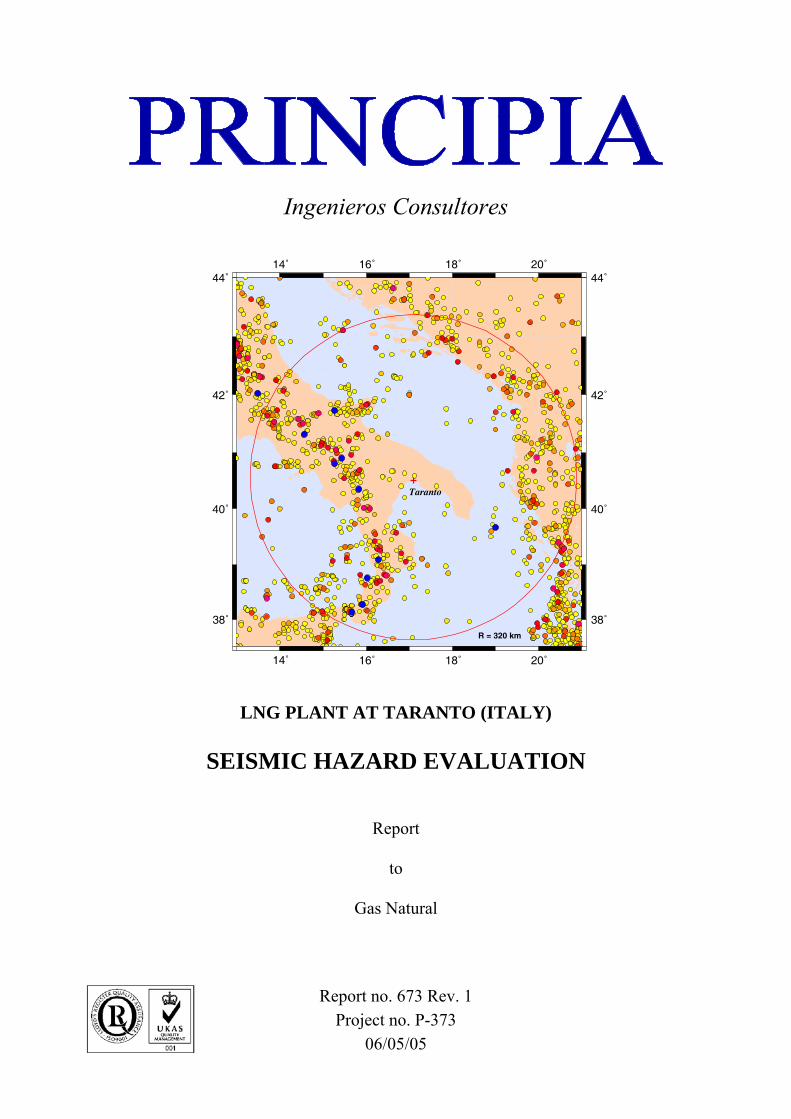
a) Compilation of the earthquake database over an area greater than a circle, centred at the site and with 320 km radius.

b) Compilation of the existing geological and tectonic information in that same area.

c) Selection of attenuation laws and other necessary correlations (i.e. magnitude-intensity) which are applicable under the local conditions.

d) If appropriate, additions to the earthquake catalogue to account for specific geological or tectonic characteristics.

e) Determination of best values for the parameters of the kernel function, responsible for the statistical smoothing of the seismic activity leading to the establishment of an activity rate at each location.


inf22645.doc 3

f) Combination of all local activity rates, using the relevant attenuation laws, to determine the seismic hazard curve. Study of the sensitivity of the results to parametric changes.

g) Determination of the peak accelerations levels, both horizontal and vertical, which are consistent with the OBE and SSE return periods.

h) Construction of site specific response spectra for the horizontal and vertical components of the OBE and SSE design spectra.

i) Generation of synthetic accelerograms matching the design spectra.

The above activities complete the definition of the design motions at the site. However, there is also a need to determine the basic characteristics of the local soil response under the design seismic motions. This involves two additional activities:

j) One-dimensional wave propagation analyses in order to calculate strain consistent properties of the ground, i.e.: the effective shear modulus and the damping ratio.

k) Evaluation of the liquefaction potential of the soil by comparing cyclic demands and cyclic resistances in the layers that may be susceptible to this problem.

1.4 Layout of report

The rest of this report comprises another five chapters and two appendices.

Chapter 2 is concerned with the geotechnical and seismic characteristics of the site and the surrounding region, as relevant for supporting the evaluation of the seismic hazard. Attenuation laws and other necessary correlations are also discussed in this chapter.

The zoneless methodology for evaluation of the seismic hazard is described and applied to the site in chapter 3. Sensitivity analyses are also conducted in order to establish the uncertainty of the results.

Having derived the hazard curve, peak accelerations are assigned in chapter 4 to the OBE and SSE events. Then, the site specific response spectra to be used in


inf22645.doc 4

design are constructed and synthetic accelerograms, matching the various spectra, are also generated in this chapter.

The local soil response is analysed in chapter 5. This includes the determination of strain-consistent properties (stiffness and damping) and evaluating the liquefaction potential of the ground.

Finally, chapter 6 summarily presents the conclusions and recommendations arising from the work conducted.

The first appendix lists the bibliographic and documentary references mentioned in the text of the report. The second one provides a summary description of the program KERFRACT used in the evaluation of the seismic hazard.


inf22645.doc 5

2. DESCRIPTION OF THE PROBLEM

2.1 Relevant norms

The following norms and guidelines have been taken into account when conducting the studies described in the present report:

– “OPCM 2003: Primi Elementi in Materia di Criteri Generali per la Classificazione Sismica del Territorio Nazionale e di Normative Tecniche per le Construzioni in Zona Sismica” (OPCM, 2003).

– “Eurocode 8: Design Provisions for Earthquake Resistance of Structures” (CEN, 1994).

– “EN 1473: Installation and Equipment for Liquefied Natural Gas. Design of Onshore Installations” (CEN, 1997).

– “NFPA 59-A: Production, Storage and Handing of Liquefied Natural Gas” (National Fire Protection Association, 1996).

2.2 General approach

The initially favoured deterministic approach for establishing design earthquakes had to be abandoned relatively soon. It required determining the maximum credible earthquake for each potential seismic source and assuming the occurrence of that event at the closest possible distance to the site. The main reason for abandoning the method was that it is very difficult indeed to determine a maximum credible earthquake, even assuming that such a concept is actually meaningful.

Instead, the seismic hazard is now evaluated using a probabilistic approach. Activity rates are assigned to each point throughout the area which may contribute significantly to the seismic hazard at the site. Attenuation laws can then be used to calculate, for the earthquakes that could occur at each point, the motions that would be felt at the site. The simultaneous consideration of the activity rates throughout the region of influence, together with the appropriate attenuation laws, yields the seismic hazard at the site.


inf22645.doc 6

The assignment of activity rates for each point within the region of influence leads to a seismic generation model. The rates must be derived on the basis of the earthquakes generated before (seismic catalogue), enlightened by the existing geological and tectonic information. The question is how to build a seismic generation model using the earthquakes in the catalogue.

The traditional procedure (Cornell, 1968) has been to use the seismic, geological and tectonic information to construct a series of non-overlapping zones, jointly spanning the region of influence (a 320 km circle). Each one of them is assumed to have a uniform seismicity. The discrete character of the information of the earthquake catalogue is smoothed by uniformly distributing over each zone the contributions to activity implied by each of the past earthquakes which took place within that zone.

This type of procedure seems logical when a strong correlation can be established between known tectonic features and past earthquake history. It also had the advantage of requiring only moderate computational resources, which was a mandatory consideration at the time of its development.

The very large increase in computational capabilities achieved over the years, though, makes it possible to reconsider whether a firm scientific basis exists for uniform seismicity zones; indeed, limited computer power no longer restricts the choice in that respect. And what is found is that the distribution of seismic activity has a far richer underlying structure than allowed by uniform seismicity zones.

Moreover, particularly in regions of moderate and low seismic activity, or with rather incomplete earthquake catalogues, the construction of the seismogenetic zones inevitably incorporates a large subjective component with potentially major implications on the results. This opens the methodology to criticism and introduces considerable uncertainty in the results.

As a consequence of these limitations, a different procedure was created (Woo, 1995, 1996a) which is the one that will be used here. Principia has already used that procedure at all other sites with LNG tanks in Spain (Crespo and Martí, 2002), as well as some LNG plants abroad like Dahej (India), Damietta (Egypt), Lázaro Cárdenas (Mexico) or Saint John (Canada).


inf22645.doc 7

Given an earthquake catalogue with epicentres, magnitudes and effective observation periods for each magnitude, an activity rate function is constructed for each location. This function arises from a statistical smoothing of the data, recognising the probabilistic nature of the discrete sample of historical observations available; the statistical smoothing, though, using kernel functions, does not require assuming a priori the existence of any kind of seismogenetic zones with a prescribed distribution of activity, uniform or otherwise. The only disadvantage of this procedure is the requirement of greater computational power, which today is only a minor drawback. In return, the reliability and objectivity of the results are considerably improved.

Additional details about the zoneless methodology are given in section 3.1 and in the references by Woo mentioned in the previous paragraphs.

2.3 Seismic information

In order to compile the seismic history that is necessary for conducting the hazard calculations, two earthquake databases have been used:

– NT 4.1 Catalogue of the Gruppo Nazionale per la Difensa dai Terremoti (GNDT, 2005). The total number of events recorded is 2488, between the years 1000 and 1992. In this catalogue, the earthquake size is described with the surface wave magnitude Ms.

– Seismic Bulletin (INGV-CNT, 2005) of the Istituto Nazionale di Geofisica e Vulcanologia and the Centro Nazionale Terremoti The total number of events recorded is 50,262, between the years 1983 and 2003. In this catalogue, the earthquake size is described with the local magnitude ML, the duration magnitude MD, or both.

These two databases have been combined in a single one, using the data from NT 4.1 up to 1983 and the Seismic Bulletin after that year. Events without an assigned magnitude have been removed, resulting in a total number of 46,862 in the combined database. Also, the magnitude adopted, referred to as M in this report, corresponds to the surface-wave magnitude Ms when both local magnitude ML and Ms are greater than or equal to 5.5 and corresponds to ML for lower magnitudes. This procedure avoids the saturation effects of ML for the larger earthquakes and coincides with the criteria adopted by Sabetta and Pugliese (1987 and 1996).


inf22645.doc 8

The Taranto site is located in the south of Italy. The site coordinates adopted for the study are:

40º 30’ North

17º 10’ East

Starting from the combined catalogue, the earthquakes selected for further consideration were those with epicentres inside the rectangle comprised between the following geographical coordinates:

– latitude: 37º 30’ to 44º 00’ North

– longitude: 13º 00’ to 21º 00’ East

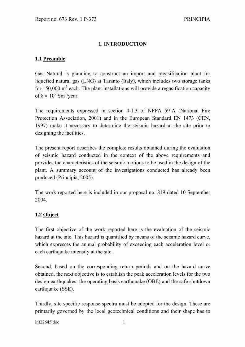
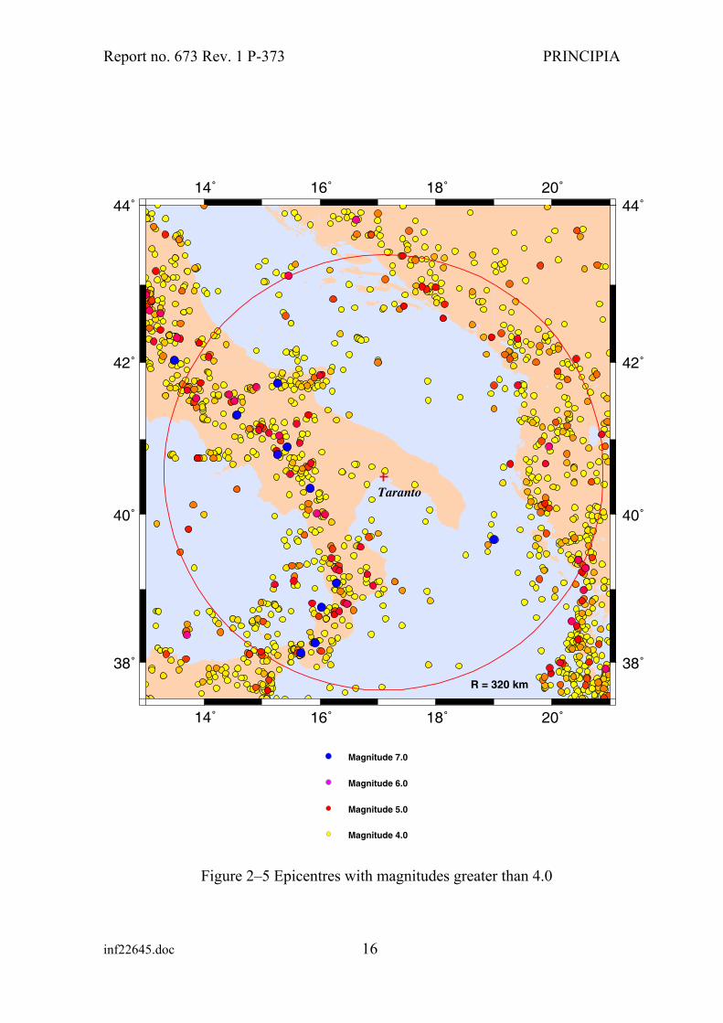
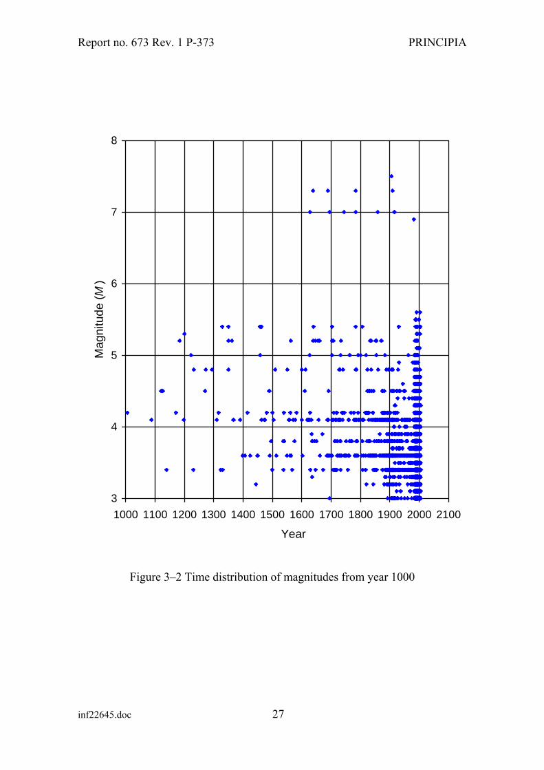
This produced a total of 2,490 earthquakes with magnitude greater than or equal to 3, excluding foreshocks, aftershocks and earthquakes without assigned magnitude or intensity. All these epicentres are shown in Figure 2–4; Figure 2–5 presents the epicentres of earthquakes with magnitude above 4.0.

2.4 Tectonic information

By comparing recent and historical seismicity, using the stress and strain fields gathered from all available data (see Figure 2–1) and the deep structure recovered from seismic tomography, seismologists have been able to set firm constraints on Italy’s active tectonics around the site (Valensise et al, 2003):

– An almost continuous seismic belt follows the buried margin of the Adriatic microplate beneath the Apennines and the Alps, and the boundary between the Ionian lithosphere and the Calabrian arc.

– A relatively narrow belt of seismicity characterizes the southern Apennines, where earthquakes are larger than in the northern arc and individual faults are up to 30-50 km long. Earthquake and active stress data consistently reflect the dominant ongoing NE-SW extension. Conversely, the role of E-W right lateral strike-slip faults revealed by recent moderate-size earthquakes and affecting the Apulian foreland is steel unclear. Such quakes may result from lateral complexities, accommodate different rates of extension, or represent the reactivation of pre-existing major faults dating back to the construction of the Apennines. The southern part of the Apennines is dominated by a detached (or


inf22645.doc 9

possibly less dense) lithographic slab, which could be the engine of the uplift and extension phenomena.

– A narrow seismic zone appears in the Calabrian arc. Shallow earthquakes are recorded inland, whereas intermediate and deep events are observed beneath the southern Tyrrhenian. The subduction zone is only 200 km wide but extends more down-dip. Intriguing features of this deep activity are the geometry of the Ionian slab, which appears to sink passively in the mantle, and the slab’s interior earthquake mechanism, consistently down-dip compression.

A fault segmentation model of Italy was developed by the Istituto Nazionale di Geofisica e Vulcanologia. The model rests on the assumption that seismicity may be approximated by a finite number of potential seismogenetic sources. It was based on available good historical data, findings from instrumental seismicity and the knowledge of active faulting in Italy.

A potential seismogenetic source is the surface projection of an inferred fault which may experience a significant earthquake in the future. Not all potential sources will have earthquakes, and not all earthquakes will necessary occur on identified potential sources, but the list of seismic sources may be useful in hazard estimation. The current release of the segmentation model (Figure 2–2) lists about 250 potential earthquake sources grouped according to their identification criteria and parameters.

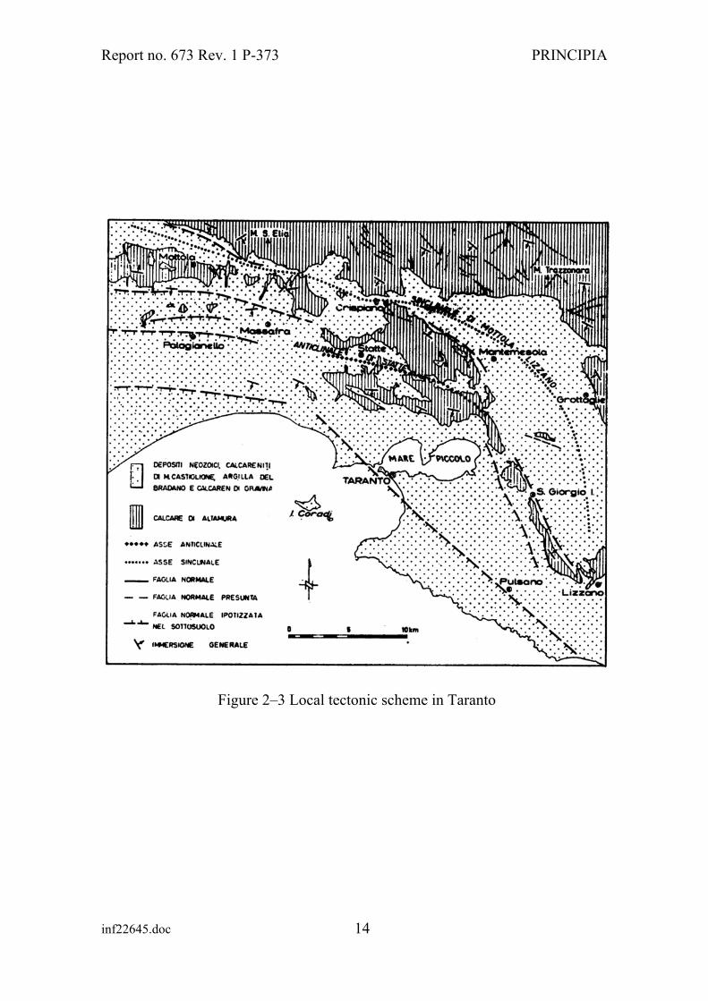
The tectonic scheme in the proximity of Taranto is dominated by a Mesozoic calcareous slab sinking under a Neozoic one. This mechanism produces faults which, even though they may not be apparent at the surface, would exist at greater depths. The local tectonic scheme is shown in Figure 2–3 (Medea, 2004).

2.5 Geotechnical site information

The geotechnical information about the site, as well as preliminary recommendations for foundation design of the onshore terminal, have been provided by Soil (2005).

Briefly, the overall soil profile can be described as follows:


inf22645.doc 10

a) Layer 1: artificial fill, gradually placed in relatively recent years over a previously submerged area. It is formed by “waste” and/or “slags”, very likely produced by adjacent iron factories.

b) Layer 2: it consists of highly overconsolidated, very stiff becoming hard clays.

c) Layer 3: between the above main formations, a layer of medium to dense sand is encountered. Its thickness is variable from 1.5 to 2.5 m.

d) Layer 4: its top part is formed by medium dense sand with silty interlayers. Its lower part is formed by sandy of clayey silt/silty clay, very likely normally consolidated.

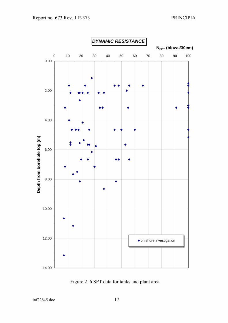
The SPT blowcounts recorded in the first 14 m are shown in Figure 2–6.

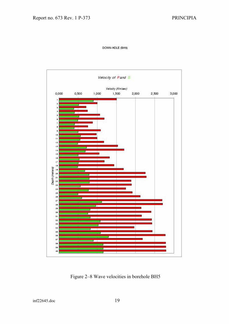
Two down-holes were conducted using boreholes at the centre of each tank base (boreholes BH1 and BH5). The compression (P) and shear (S) wave velocities obtained in the two boreholes are presented in Figure 2–7 and Figure 2–8.

2.6 Attenuation laws

The energy liberated in the focal area of the earthquake will propagate in all directions in the form of waves, which will expand with distance and, consequently, will increase their amplitude.

Besides the geometrical attenuation mentioned, there will be other effects arising from inelasticity of the deforming materials as well as from the geometrical distribution of impedance, which gives arise to reflections, refractions and varying propagation velocities.

Because of all the latter factors, attenuation laws are usually dependent on the earthquake magnitude, hypocentral depth and geological characteristics of the region. Hence, where possible, locally applicable attenuation laws are used, which also take into account the dependence on focal depth and earthquake magnitude.


inf22645.doc 11

For the present evaluation of the seismic hazard, the attenuation law proposed by Sabetta and Pugliese (1987 and 1996) for the Italian region are particularly applicable and have therefore been used. Their law is expressed in terms of the magnitude M explained in section 2.3. The attenuation law is shown in Figure 2–9 and can be written as:

log y = a + bM – log (R2 + h2)½ + eS (2–1)

where y is acceleration

R is the epicentral distance

S = 0 for stiff and deep soil sites and S = 1 for shallow soil sites

a, b, e and h are empirical constants, for which the values obtained by Sabetta and Pugliese have been adopted.

2.7 Other correlations used

In order to carry out the evaluation of the seismic hazard, correlations must be established between the different measures of earthquake magnitude. This is because different magnitude measures are quoted in the earthquake catalogues.

The Ms-ML correlation applied here is the same one used by the NT 4.1 Catalogue of the Gruppo Nazionale per la Difensa dai Terremoti:

Ms = 1.25ML - 1.39 (2–2)

obtained with a sample of 93 events with a standard deviation of 0.27.

In order to develop a correlation between ML and MD, use has been the 27,651 events for which both magnitude measures had an assigned value. Then, a least-square fit of the data has been conducted. The resulting correlation corresponds to the following equation:

ML = 0.979MD - 0.500 (2–3)


Figure 2–1 Active stress map and locations of significant recent earthquakes

inf22645.doc 12


Figure 2–2 Main trends of identified seismogenetic sources

inf22645.doc 13


Figure 2–3 Local tectonic scheme in Taranto

inf22645.doc 14


14˚

14˚

16˚

16˚

18˚

18˚

20˚

20˚

38˚ 38˚

40˚ 40˚

42˚ 42˚

44˚ 44˚

Taranto

R = 320 km

Figure 2–4 Epicentres from the catalogue

inf22645.doc 15


14˚

14˚

16˚

16˚

18˚

18˚

20˚

20˚

38˚ 38˚

40˚ 40˚

42˚ 42˚

44˚ 44˚

Taranto

R = 320 km

Magnitude 7.0

Magnitude 6.0

Magnitude 5.0

Magnitude 4.0

Figure 2–5 Epicentres with magnitudes greater than 4.0

inf22645.doc 16


DYNAMIC RESISTANCE

0.00

2.00

4.00

6.00

8.00

10.00

12.00

14.00

0 10 20 30 40 50 60 70 80 90 100

NSPT (blows/30cm)

Dep

th fr

om b

oreh

ole

top

(m)

on shore investigation

Figure 2–6 SPT data for tanks and plant area

inf22645.doc 17


Figure 2–7 Wave velocities in borehole BH1

inf22645.doc 18


Figure 2–8 Wave velocities in borehole BH5

inf22645.doc 19


0.001

0.010

0.100

1.000

1 10

Distance (km)

Acc

eler

atio

n (g

)

100

Magnitude 3.0Magnitude 4.0Magnitude 5.0

Figure 2–9 Attenuation law by Sabetta and Pugliese (1987 and 1996)

inf22645.doc 20


3. EVALUATION OF THE HAZARD

3.1 Description of the methodology

The zoneless method used follows the ideas proposed by Woo (1995, 1996a). The numerical implementation is that embodied in the computer program KERFRACT (Woo, 1996b). The procedure is the same one already employed for determining the seismic hazard at all other sites with LNG tanks in Spain (Crespo and Martí, 2002).

The basic starting data are the catalogue of past epicentres and their corresponding magnitudes, together with the knowledge of the effective period of observation for each magnitude. This will allow constructing an activity rate for each location and event magnitude.

The estimated activity rate must take into account the probabilistic nature of the discrete sample provided by the catalogue. This is introduced by a statistical smoothing of the data. The activity rate is obtained by adding the individual contributions of all events in the catalogue. The smoothing is achieved by means of a kernel function and takes into account the return period of the event under consideration. More specifically, the activity rate is expressed:

)(

),(),( 1

i

N

ii

T

MKM

x

xxx

∑=

−=λ (3–1)

where M is the magnitude of the event x are the coordinates of the location where the activity rate is being calculated

xi are the coordinates of the epicentre being considered

K is the kernel function

T is the return period associated to the event the contribution of which is being considered

A factorised form of the kernel function is used, which can have an isotropic character or a directional dependence. A Gaussian dependence on distance allows

inf22645.doc 21


incorporating naturally the inevitable uncertainty associated with epicentral locations. However, a power-law dependence is the one that arises from the fractal character of earthquake generation.

Here, an isotropic form of the kernel function, with a power-law dependence on distance, will be used for the evaluation. The kernel function K takes the form:

n

Hr

HnK

−

⎥⎦

⎤⎢⎣

⎡⎟⎠⎞

⎜⎝⎛−−=

2

2 11π (3–2)

where n is the exponent of the power-law

H is a bandwidth for normalising distances

r is the distance to the epicentre

The exponent n depends on proximity between epicenters, increasing with proximity. Its value, which typically lies between 1.5 and 2, has only a moderate influence on the results. Values as low as 1.25 are possible but n cannot be less than 1. The kernel function, as the normalized distance r/H increases, goes to zero with the -2n power of the normalized distance.

The bandwidth H is a function of magnitude. It represents the minimum distance between epicenters of the same magnitude. Its relation with magnitude takes an exponential form:

H = c e dM (3–3)

where c and d are constants to be determined on the basis of the epicentres contained in the catalogue

M is the magnitude employed in the attenuation relation.

3.2 Specification of the kernel function

As has been described, the kernel function is completely defined when the bandwidth and the power-law exponent are specified. The bandwidth is an exponential function of magnitude (see eq. 3–3) which involves two constants (c and d).

inf22645.doc 22


inf22645.doc 23

For the case under consideration, based on the epicentres located within a circle centred at Taranto and with a 320 km radius, the following steps were taken:

a) Events are classified in groups according to their magnitude.

b) For each event, the distance to the nearest epicentre within the same magnitude range is determined.

c) All minimum distances calculated for each magnitude range are averaged.

d) A least-square fit is conducted in order to obtain the two parameters c and d that appear in equation 3–3: c = 0.043 km and d = 1.229.

Figure 3–1 presents the best fit of the catalogue data using a straight line. The line is characterised by its two parameters, which have in this case the values c = 0.043 km and d = 1.229. Since the fit is fairly good, it is not considered necessary to conduct sensitivity analyses with respect to these values. However, the power-law exponent n will be the subject of a sensitivity analysis.

3.3 Effective detection periods

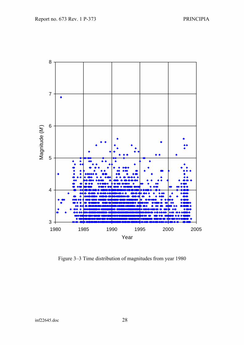
Each event must be assigned a period of observation depending on its magnitude, that is, an effective historical threshold for potentially recording it if it had occurred. A temporal distribution of the events in the catalogue is shown in Figure 3–2 for all events and in Figure 3–3 for the more recent ones.

The procedure by Woo (1996b) requires assigning a reference year to each earthquake; this measures the probability of detecting earthquakes of identical characteristics at different times in history. The reference year depends on the specific characteristics of the earthquake. The following aspects will be taken into account:

– magnitude M

– epicentral location: onshore or offshore

– year of occurrence

Earthquakes sharing the three criteria above will have the same reference year assigned to them.


The magnitude and year of occurrence of each earthquake are taken into account for determining the effective period of the earthquake as follows:

a) History is divided into time intervals as a function of the means of detection available at each time.

b) For each interval with duration Di and each level of magnitude M, a probability of detection pim is estimated based on the possibilities offered by the available technology.

c) A reference year Am is established for each magnitude level:

∑−=i

iim0m DpAA (3–3)

where A0 is the earliest year with records

The process is carried out separately for onshore and offshore epicentres. It is assumed that the latter only became detectable in the instrumental era and have therefore a zero probability of detection before that time.

Having conducted this exercise, the reference years assigned to the various earthquakes appear in Table 3–1.

Onshore earthquakes Offshore earthquakes

Magnitude Reference year Magnitude Reference year

> 5.5 1425 > 5.5 1825

5.0 – 5.5 1650 5.0 – 5.5 1825 4.5 – 5.0 1825 4.5 – 5.0 1855 4.0 – 4.5 1895 4.0 – 4.5 1916 3.5 – 4.0 1916 3.5 – 4.0 1953 3.0 – 3.5 1962 3.0 – 3.5 1974

Table 3–1 Reference years for different event intensities

inf22645.doc 24


inf22645.doc 25

3.4 Seismic hazard at the site

The application of the methodology described in earlier sections yields results, directly in terms of acceleration, for each return period or annual probability of exceedance. The attenuation law used corresponds to the shallow soil type proposed by Sabetta and Pugliese (1987 and 1996), as explained in section 2.6. The accelerations obtained are referred to zero period.

The hazard curve, relating the accelerations to the different probabilities of occurrence, is shown in Figure 3–4. The main assumptions used in its derivation are:

– Exponent in the kernel function: n = 1.75.

– Bandwidth parameters: c = 0.043 km and d = 1.229.

The bandwidth parameters had very little uncertainty and there is therefore little justification for studying the sensitivity of the results to variations in those parameters. The exponent of the power law, however, is slightly more uncertain. Hence, apart from the central value n = 1.75, the calculations were repeated with 1.50 and with 2. The corresponding curves are all plotted together in Figure 3–5; as can be seen, the effects of the variation of the power-law exponent over its probable range are very small, thereby strengthening the reliability of the findings.


1

10

100

2 3 4 5 6 7

Magnitude (M s)

Ban

dwid

th (k

m)

Data

c = 0.043, d = 1.229

Figure 3–1 Curve-fits for bandwidth

inf22645.doc 26


3

4

5

6

7

8

1000 1100 1200 1300 1400 1500 1600 1700 1800 1900 2000 2100

Year

Mag

nitu

de (M

)

Figure 3–2 Time distribution of magnitudes from year 1000

inf22645.doc 27


3

4

5

6

7

8

1980 1985 1990 1995 2000 2005Year

Mag

nitu

de (M

)

Figure 3–3 Time distribution of magnitudes from year 1980

inf22645.doc 28


0.0001

0.0010

0.0100

0.1000

1.0000

0.00 0.05 0.10 0.15 0.20 0.25 0.30

Acceleration (g)

Pro

babi

lity

of e

xcee

danc

e (y

ear -1

)

Figure 3–4 Spectral acceleration, T = 0 s

inf22645.doc 29


0.0001

0.0010

0.0100

0.1000

1.0000

0.00 0.05 0.10 0.15 0.20 0.25 0.30

Acceleration (g)

Pro

babi

lity

(yea

r -1)

n = 1.50n = 1.75n = 2.00

Figure 3–5 Sensitivity to the power-law exponent

inf22645.doc 30


inf22645.doc 31

4. DESIGN MOTIONS

4.1 Design accelerations

The seismic hazard curve for the site was already derived in the previous chapter. For design, though, this information must be combined with the corresponding periods in order to arrive at the peak ground accelerations for the OBE and SSE motions.

The return periods for the two design earthquakes are 475 years for the OBE and 10,000 years for the SSE. This latter period was the one adopted by the NFPA 59–A until 2001 and that EN 1473 still maintains. This period can be considered conservative, since the revised NFPA 59–A reduces it. In any case, a higher rank is assigned to EN 1473 for this project.

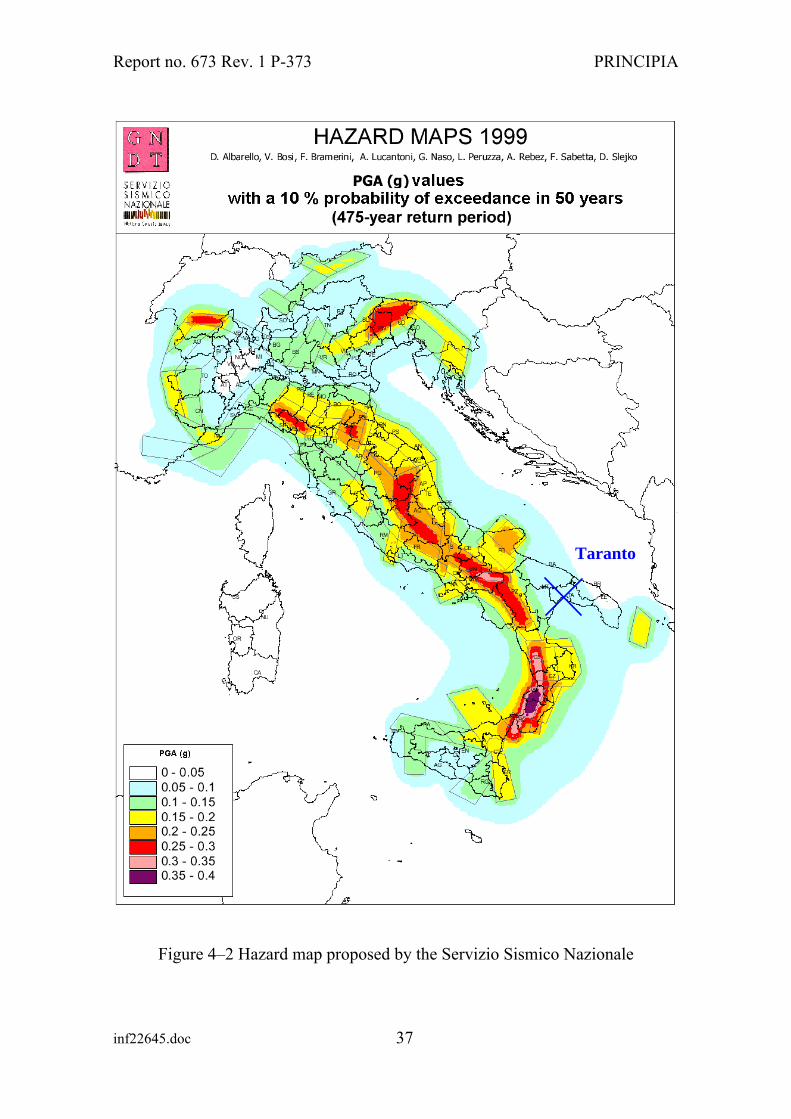
As can be checked in Figure 4–1, the peak ground accelerations consistent with the above return periods are 0.09g for the OBE and 0.29g for the SSE. The acceleration resulting for the 475 year return period is in the range established by the OPCM (2003) for Taranto (code 16073027, zone 3); the Italian norm assigns values comprised between 0.05g and 0.15g for this site. The OBE acceleration is also consistent with the findings of the Servizio Sismico Nazionale presented in Figure 4–2.

4.2 Site specific response spectra

The response spectrum describes the frequency distribution of the ground motion. It is defined as the motion amplification that an elementary oscillator would experience as a function of the frequency to which it was tuned.

OPCM (2003) establishes five soil profiles, characterised in terms of the local values of the shear wave velocity. In this study spectra and matching accelerograms will be developed for a soil classified as type B in OPCM (2003); this decision is consistent with the results of the geotechnical investigation conducted at the site (Soil, 2005), which was already presented succinctly in section 2.5. This soil type consists of deposits of very dense sand, gravel, or very stiff clay, at least several tens of metres in thickness, characterized by a gradual


increase of mechanical properties with depth; the average shear wave velocity in the top 30 meters is between 360 and 800 m/s.

For each soil profile, OPCM (2003) defines the spectral shape by means of four segments. In the present case the four segments of the spectrum are described by the following equations, depending on the period T:

a) for T<TB

)15.2(0.1)(

−⋅⋅+=⋅

ηBg

e

TT

aSTS (4–1)

b) for TB<T<TC

5.2)(

⋅=⋅

ηg

e

aSTS

(4–2)

c) for TC<T<TD

⎟⎠⎞

⎜⎝⎛⋅⋅=

⋅ TT

aSTS C

g

e 5.2)(

η (4–3)

d) for TD<T

⎟⎠⎞

⎜⎝⎛ ⋅

⋅⋅=⋅ 25.2

)(T

TTaSTS DC

g

e η (4–4)

The damping correction factor η(ξ) is expressed as a function of the damping ratio ξ by means of the equation:

ξη

+=

510 (4–5)

and cannot be lower than 0.55.

In the previous expressions, S⋅ag is the maximum acceleration of the soil of the site as is discussed in section 4.1, where the factor S = 1.25 takes into account the soil profile; TB and TC depend on the ground characteristics (in the present case inf22645.doc 32


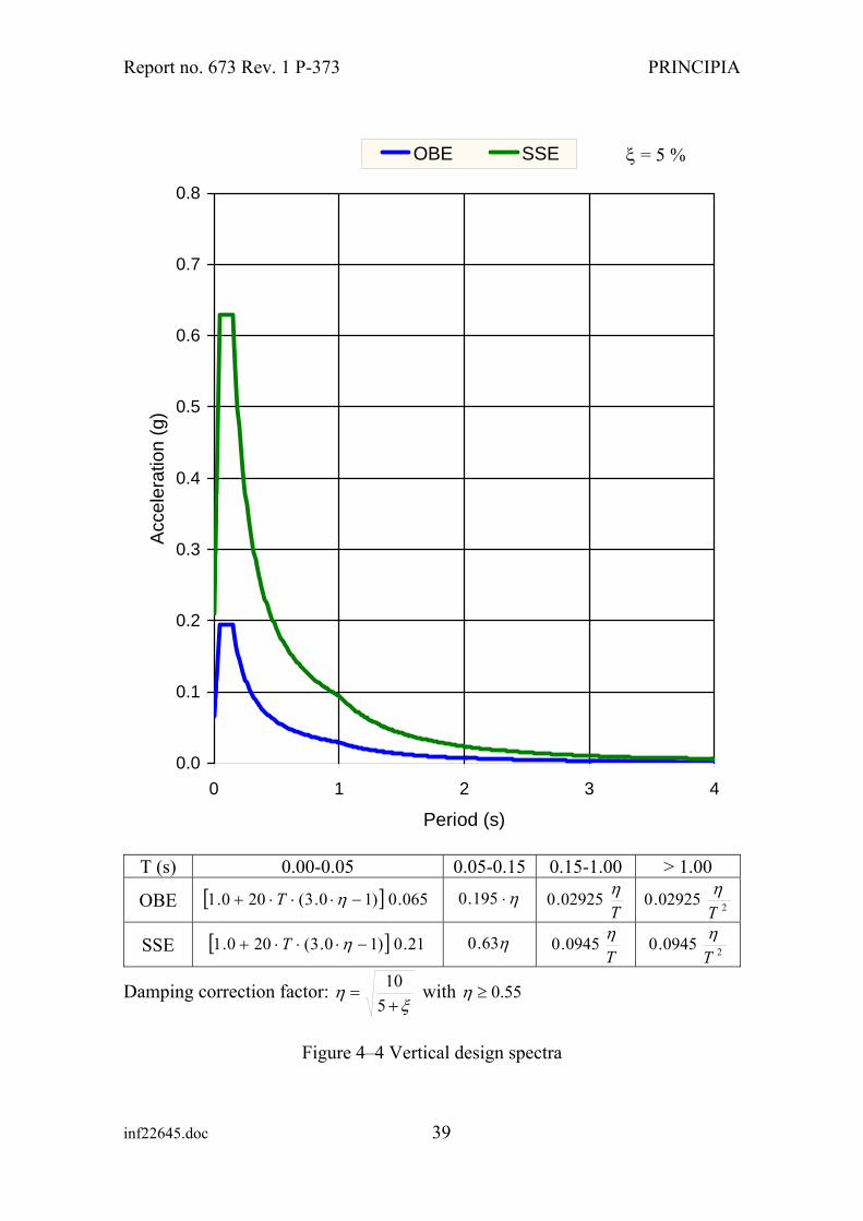
TB = 0.15 s and TC = 0.5 s) and TD = 2 s is the period beyond which the spectrum corresponds to constant displacement. The horizontal spectra for the OBE and SSE with ξ = 5% are presented in Figure 4–3.

The spectrum of the vertical motions is defined in the OPCM (2003) as:

a) for T<TBV

⎥⎦

⎤⎢⎣

⎡−⋅+⋅⋅=

⋅)10.3(0.19.01)(

ηBV

Vg

eV

TTS

SaSTS (4–6)

b) for TBV<T<TCV

0.39.01)(⋅⋅⋅⋅=

⋅ηV

g

eV SSaS

TS

(4–7)

c) for TCV<T<TDV

⎟⎠⎞

⎜⎝⎛⋅⋅⋅⋅⋅=

⋅ TT

SSaS

TS CVV

g

eV 0.39.01)(η

(4–8)

d) for TDV<T

⎟⎠⎞

⎜⎝⎛⋅⋅⋅⋅⋅=

⋅ 20.39.01)(T

TTS

SaSTS DVCV

Vg

eV η (4–9)

In this case SV = 1.0, TBV = 0.05 s, TCV = 0.15 s and TDV = 1.0 s.

The vertical spectra for the OBE and SSE with ξ = 5% are presented in Figure 4–4.

4.3 Matching accelerograms

For the generation of synthetic accelerograms, besides the accelerations and spectra already produced, it is necessary to specify durations. In order to arrive at a duration, the more probable magnitudes an epicentral distances have been found for both the OBE and SSE. The results were:

inf22645.doc 33


inf22645.doc 34

– for the OBE: magnitude 5.5 at 24 km

– for the SSE: magnitude 6.9 at 24 km

Having done that, a number of correlations from the specialised literature were employed to evaluate the more probable durations of the motions. The dispersion of the predictions arising from the various correlations is a reflection of the considerable uncertainty involved in such formulae.

For the total OBE duration, the results produced using the various correlations are:

– Esteva and Rosenblueth (1964): 8 s

– Housner (1965): 9 s

– Dobry et al (1978): 3 s

– Trifunac and Brady (1975): 12 s

For the total SSE duration, the corresponding results follow:

– Esteva and Rosenblueth (1964): 11 s

– Housner (1965): 24 s

– Dobry et al (1978): 14 s

– Trifunac and Brady (1975): 15 s

However, the new Italian norm has a fairly conservative approach to the specification of earthquake durations for small and moderate events, as it prescribes a minimum duration of 25 s for all events. This duration is greater than any of the ones predicted by existing correlations and has therefore been the one adopted for both the OBE and the SSE motions.

The generation of synthetic accelerograms has relied on the use of the following software:

– SIMQKE (Gasparini, 1975), which generates accelerograms that approximately fit the target response spectrum.


inf22645.doc 35

– POSTQUAKE (Woo, 1987), a program based on the methodology proposed by Kaul (1978), which modifies the SIMQKE generated accelerogram to decrease the deviations from the target spectrum to below a specified tolerance (10% in this case).

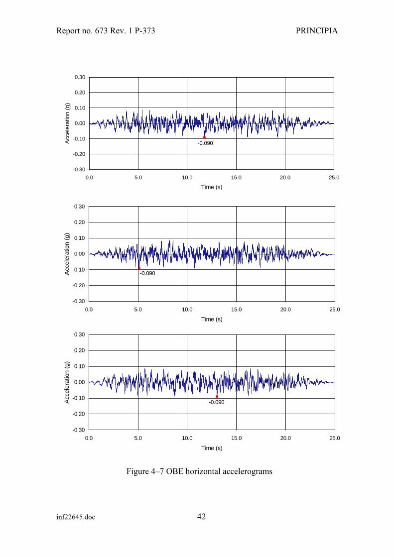
The history of motions must be distributed in three phases: increasing motions (increasing ramp), strong motions (plateau) and decreasing motions (decreasing ramp). The total duration has been distributed in the same fashion for both the OBE and the SSE accelerograms. The durations of each of the three phases mentioned are:

– Increasing ramp: 5.0 s

– Plateau: 12.5 s

– Decreasing ramp: 7.5 s

As requested by the Italian norm, three different accelerograms have been generated for each of the four design spectra presented in Figures 4–3 and 4–4; they appear in Figures 4–5 to 4–6 for the SSE and 4–7 and 4–8 for the OBE. The synthetic accelerograms satisfy the criteria given in ASCE Standard 4-98 (ASCE, 1999).

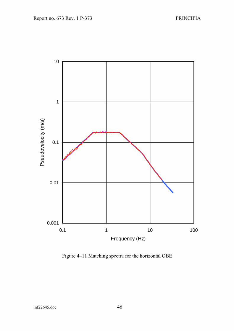
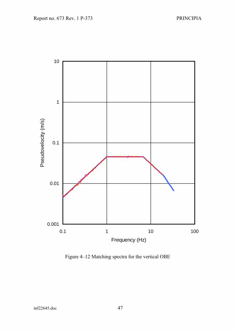
Figures 4–9 to 4–12 superimpose, for each of the four earthquake types of interest, the target spectra and the spectra corresponding to the synthetic accelerograms. It is clear that the spectra of the accelerograms provide in each case a very good fit of the target design spectra.

It should be noticed that the accelerograms generated fit the design spectra for a 5% damping ratio, which is an intermediate value among the structural dampings found in the tank. It is well known that a good fit for a certain damping value does not guarantee that this will be maintained for other values; the approximation usually deteriorates as the damping difference increases. As a consequence, if the damping ratio differs significantly from 5%, the accelerograms provided should not be used without verifying that the approximation to the target spectrum is acceptable for the damping ratio of interest.


inf22645.doc 36


inf22645.doc 36

0.0001

0.0010

0.0100

0.1000

1.0000

0.00 0.05 0.10 0.15 0.20 0.25 0.30

Acceleration (g)

Pro

babi

lity

of e

xcee

danc

e (y

ear -1

)

0.0001

0.0010

0.0100

0.1000

1.0000

0.00 0.05 0.10 0.15 0.20 0.25 0.30

Acceleration (g)

Pro

babi

lity

of e

xcee

danc

e (y

ear -1

)

Figure 4–1 Design accelerations


Figure 4–2 Hazard map proposed by the Servizio Sismico N

inf22645.doc 37

Taranto

azionale


0.0

0.1

0.2

0.3

0.4

0.5

0.6

0.7

0.8

0 1 2 3

Period (s)

Acc

eler

atio

n (g

)

4

OBE SSE ξ = 5 %

T (s) 0.00-0.15 0.15-0.50 0.50-2.00 > 2.00

OBE 09.0)15,2(3

200.1 ⎥⎦⎤

⎢⎣⎡ −+ ηT η225.0

Tη1125.0 2225.0

Tη

SSE 29.0)15,2(3

200.1 ⎥⎦⎤

⎢⎣⎡ −+ ηT η725.0

Tη3625.0 2725.0

Tη

Damping correction factor: ξ

η+

=510 with 55.0≥η

Figure 4–3 Horizontal design spectra

inf22645.doc 38


0.0

0.1

0.2

0.3

0.4

0.5

0.6

0.7

0.8

0 1 2 3

Period (s)

Acc

eler

atio

n (g

)

4

OBE SSE ξ = 5 %

T (s) 0.00-0.05 0.05-0.15 0.15-1.00 > 1.00

OBE [ ] 065.0)10.3(200.1 −⋅⋅⋅+ ηTTη02925.0

inf22645.doc 39

η⋅195.0 202925.0Tη

SSE [ ] 21.0)10.3(200.1 −⋅⋅⋅+ ηTTη0945.0 20945.0

Tη η63.0

Damping correction factor: ξ

η+

=510 with 55.0≥η

Figure 4–4 Vertical design spectra


0.290

-0.30

-0.20

-0.10

0.00

0.10

0.20

0.30

0.0 5.0 10.0 15.0 20.0

Time (s)

Acc

eler

atio

n (g

)

-0.290-0.30

-0.20

-0.10

0.00

0.10

0.20

0.30

0.0 5.0 10.0 15.0 20.0 25.0

Time (s)

Acc

eler

atio

n (g

)

-0.290-0.30

-0.20

-0.10

0.00

0.10

0.20

0.30

0.0 5.0 10.0 15.0 20.0

Time (s)

Acc

eler

atio

n (g

)

Figure 4–5 SSE horizontal accelerograms

inf22645.doc 40


0.210

-0.30

-0.20

-0.10

0.00

0.10

0.20

0.30

0.0 5.0 10.0 15.0 20.0 25.0

Time (s)

Acc

eler

atio

n (g

)

0.210

-0.30

-0.20

-0.10

0.00

0.10

0.20

0.30

0.0 5.0 10.0 15.0 20.0 25.0

Time (s)

Acc

eler

atio

n (g

)

0.210

-0.30

-0.20

-0.10

0.00

0.10

0.20

0.30

0.0 5.0 10.0 15.0 20.0 25.0

Time (s)

Acc

eler

atio

n (g

)

Figure 4–6 SSE vertical accelerograms

inf22645.doc 41


-0.090

-0.30

-0.20

-0.10

0.00

0.10

0.20

0.30

0.0 5.0 10.0 15.0 20.0 25.0

Time (s)

Acc

eler

atio

n (g

)

-0.090

-0.30

-0.20

-0.10

0.00

0.10

0.20

0.30

0.0 5.0 10.0 15.0 20.0 25.0

Time (s)

Acc

eler

atio

n (g

)

-0.090

-0.30

-0.20

-0.10

0.00

0.10

0.20

0.30

0.0 5.0 10.0 15.0 20.0 25.0

Time (s)

Acc

eler

atio

n (g

)

Figure 4–7 OBE horizontal accelerograms

inf22645.doc 42


0.0650

-0.30

-0.20

-0.10

0.00

0.10

0.20

0.30

0.0 5.0 10.0 15.0 20.0 25.0

Time (s)

Acc

eler

atio

n (g

)

OBE vertical

-0.0650

-0.30

-0.20

-0.10

0.00

0.10

0.20

0.30

0.0 5.0 10.0 15.0 20.0 25.0

Time (s)

Acce

lera

tion

(g)

0.0650

-0.30

-0.20

-0.10

0.00

0.10

0.20

0.30

0.0 5.0 10.0 15.0 20.0 25.0

Time (s)

Acc

eler

atio

n (g

)

Figure 4–8 OBE vertical accelerograms

inf22645.doc 43


0.001

0.01

0.1

1

10

0.1 1 10 100

Frequency (Hz)

Pse

udov

eloc

ity (m

/s)

Figure 4–9 Matching spectra for the horizontal SSE

inf22645.doc 44


0.001

0.01

0.1

1

10

0.1 1 10 100

Frequency (Hz)

Pse

udov

eloc

ity (m

/s)

Figure 4–10 Matching spectra for the vertical SSE

inf22645.doc 45


0.001

0.01

0.1

1

10

0.1 1 10 100

Frequency (Hz)

Pse

udov

eloc

ity (m

/s)

Figure 4–11 Matching spectra for the horizontal OBE

inf22645.doc 46


0.001

0.01

0.1

1

10

0.1 1 10 100

Frequency (Hz)

Pse

udov

eloc

ity (m

/s)

Figure 4–12 Matching spectra for the vertical OBE

inf22645.doc 47


inf22645.doc 48

5. LOCAL SOIL RESPONSE

Based on the design movements given in the previous chapter and on the geotechnical characteristics of the ground, strain-compatible dynamic properties have been calculated for the seismic motions of interest.

This information is particularly important when evaluating the dynamic stiffness of the foundation, as required for conducting soil-structure interaction analyses of the tank.

At the same time, the effective stress levels developed in the soil during each earthquake are calculated. The liquefaction potential is then investigated by comparing the calculated stress demands with the soil capacity when subjected to cyclic loads.

5.1 Idealised cross-section

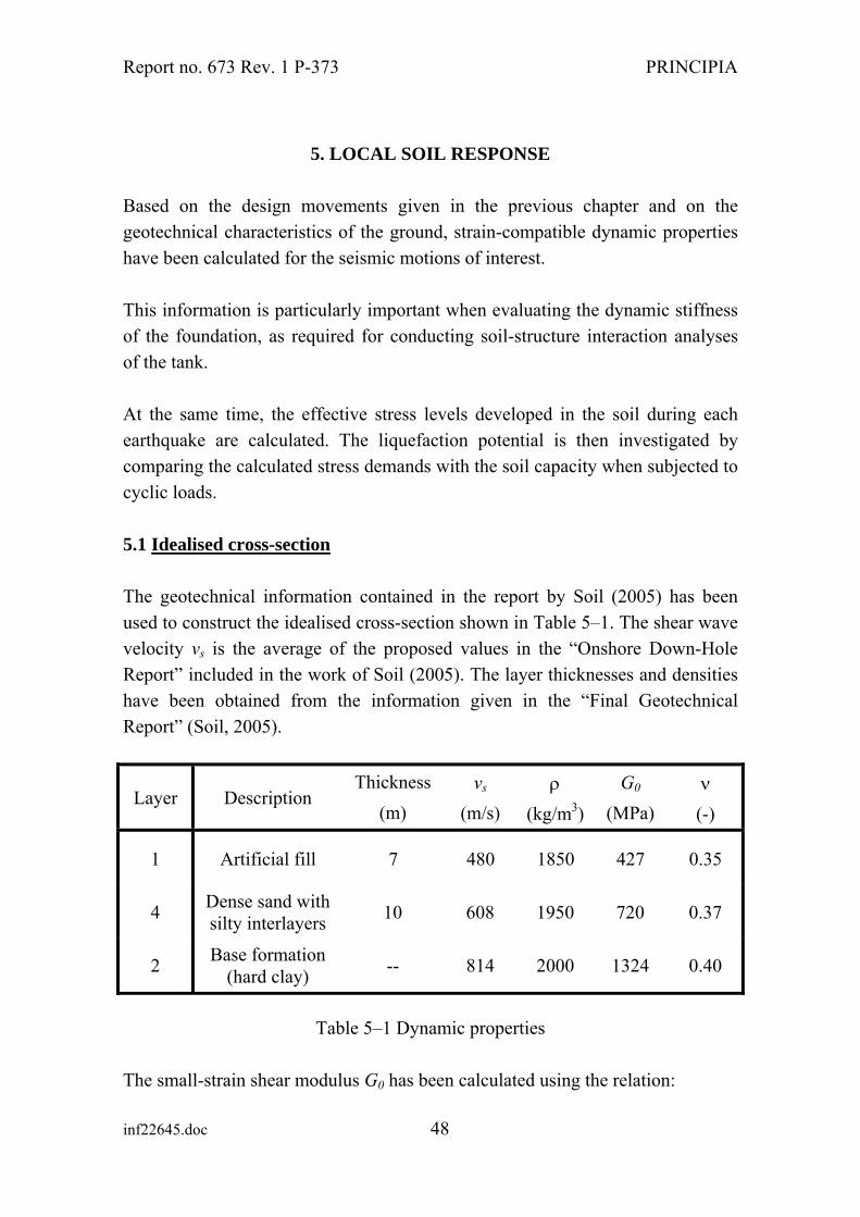
The geotechnical information contained in the report by Soil (2005) has been used to construct the idealised cross-section shown in Table 5–1. The shear wave velocity vs is the average of the proposed values in the “Onshore Down-Hole Report” included in the work of Soil (2005). The layer thicknesses and densities have been obtained from the information given in the “Final Geotechnical Report” (Soil, 2005).

Layer Description Thickness

(m) vs

(m/s) ρ

(kg/m3)

G0

(MPa) ν

(-)

1 Artificial fill 7 480 1850 427 0.35

4 Dense sand with silty interlayers 10 608 1950 720 0.37

2 Base formation (hard clay) -- 814 2000 1324 0.40

Table 5–1 Dynamic properties

The small-strain shear modulus G0 has been calculated using the relation:


2s0 vG ρ= (5–1)

where ρ is the density vs is the shear wave velocity

5.2 Dynamic response of the ground

The evaluations of the dynamic response of the ground were based on a representative soil column, with the thicknesses and shear moduli indicated in Table 5–1.

The analysis of the vertical propagation of shear waves has been carried out with the computer program SHAKE (Schnabel et al, 1972).

The seismic input consisted in each case of the two sets of the 3 accelerograms presented in the previous section, representing the horizontal motions of the OBE and the SSE, respectively. Each of these accelerograms was individually imposed to the soil column.

For the strain dependence of the shear modulus and of the hysteretic damping, the recommendations of ASCE Standard 4-98 (ASCE, 1999) were adopted; they are plotted in Figure 5–1.

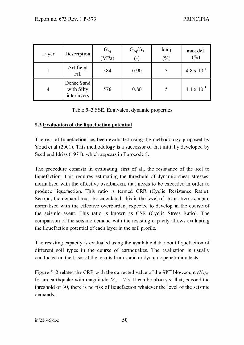
The results of the calculations for the soil profile studied are presented in Table 5–2 for the OBE and Table 5–3 for the SSE. In both cases, the tables show the averages of the results obtained for each of the three accelerograms within the corresponding group.

Layer no.

Layer description

Geq (MPa)

Geq/G0 (-)

damping

(%) max def.

(%)

1 Artificial fill 414 0.97 1.5 1.3 x 10-3

4 Dense sand with silty interlayers

662 0.92 2.5 3.0 x 10-3

Table 5–2 OBE. Equivalent dynamic properties

inf22645.doc 49


inf22645.doc 50

Layer Description Geq

(MPa) Geq/G0

(-) damp (%)

max def. (%)

1 Artificial Fill 384 0.90 3 4.8 x 10-3

4 Dense Sand with Silty interlayers

576 0.80 5 1.1 x 10-3

Table 5–3 SSE. Equivalent dynamic properties

5.3 Evaluation of the liquefaction potential

The risk of liquefaction has been evaluated using the methodology proposed by Youd et al (2001). This methodology is a successor of that initially developed by Seed and Idriss (1971), which appears in Eurocode 8.

The procedure consists in evaluating, first of all, the resistance of the soil to liquefaction. This requires estimating the threshold of dynamic shear stresses, normalised with the effective overburden, that needs to be exceeded in order to produce liquefaction. This ratio is termed CRR (Cyclic Resistance Ratio). Second, the demand must be calculated; this is the level of shear stresses, again normalised with the effective overburden, expected to develop in the course of the seismic event. This ratio is known as CSR (Cyclic Stress Ratio). The comparison of the seismic demand with the resisting capacity allows evaluating the liquefaction potential of each layer in the soil profile.

The resisting capacity is evaluated using the available data about liquefaction of different soil types in the course of earthquakes. The evaluation is usually conducted on the basis of the results from static or dynamic penetration tests.

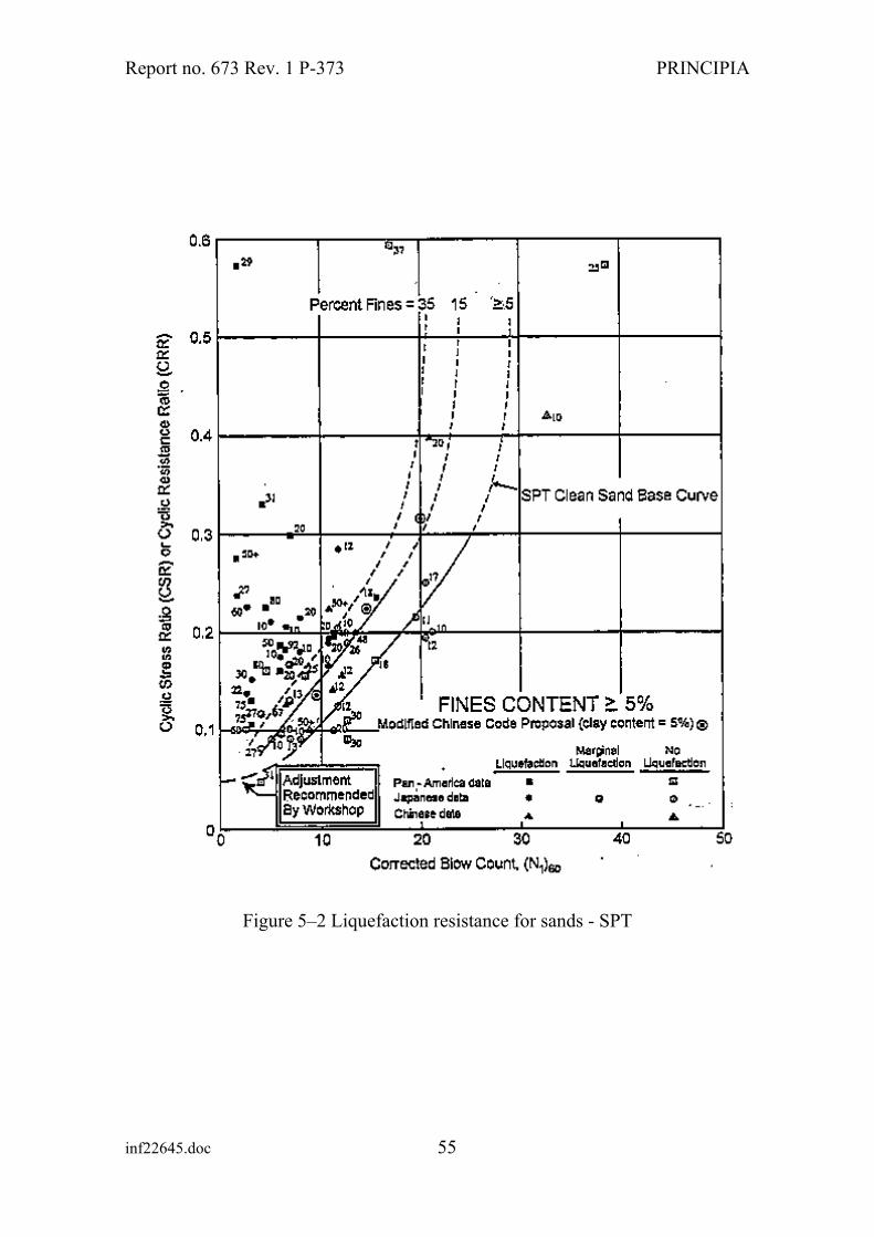
Figure 5–2 relates the CRR with the corrected value of the SPT blowcount (N1)60 for an earthquake with magnitude Mw = 7.5. It can be observed that, beyond the threshold of 30, there is no risk of liquefaction whatever the level of the seismic demands.


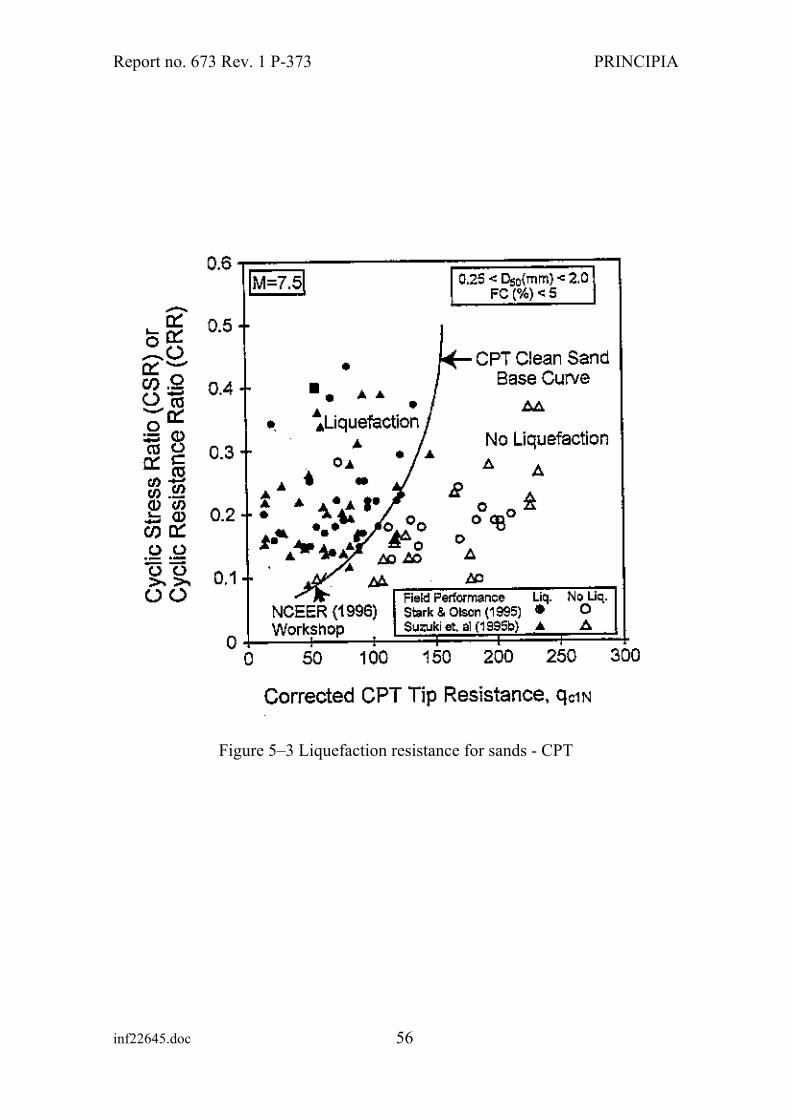
In the present study, use will also be made of the correlation between the CRR and the results of the Cone Penetration Test (CPT), since this is only the available test for layer 4.

The corrected value of (N1)60 is computed using the following expression (Youd et al, 2001):

( )5.0

0'1 ⎟

⎠⎞

⎜⎝⎛=

v

a60

pNNσ

(5–2)

where pa is the atmospheric pressure, approximately 100 kPa is the preexisting vertical effective pressure '

0vσ

The corrections used for the CPT results are too complex and will not be included here. Interested readers are referred to the work by Youd et al (2001).

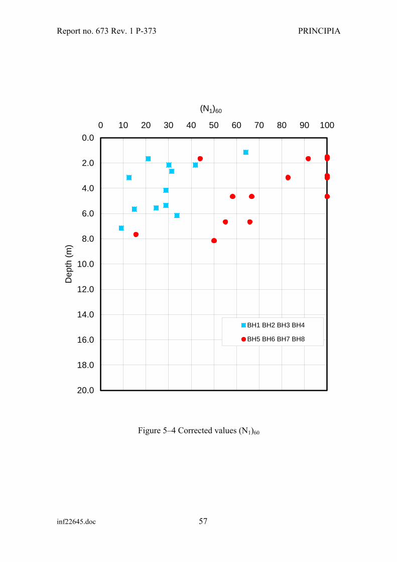
The corrected values of (N1)60 for all boreholes under the two tanks appear in Table 5–4 and have also been plotted in Figure 5–4. Boreholes 1 to 4 correspond to tank 1 and BH 5 to 8 are located under tank 2. It can be noticed that the tendencies are somewhat different below each tank. The table shows the average value of (N1)60 for each tank and for all the borehole data. The lower and upper bounds, also presented in the table, have been obtained by adding and subtracting one standard deviation to the mean value.

Boreholes Lower bound Average Upper

bound

1-4 13 28 43 5-8 50 77 > 100

1-8 23 56 89

Table 5–4 Lower, average and upper values of (N1)60

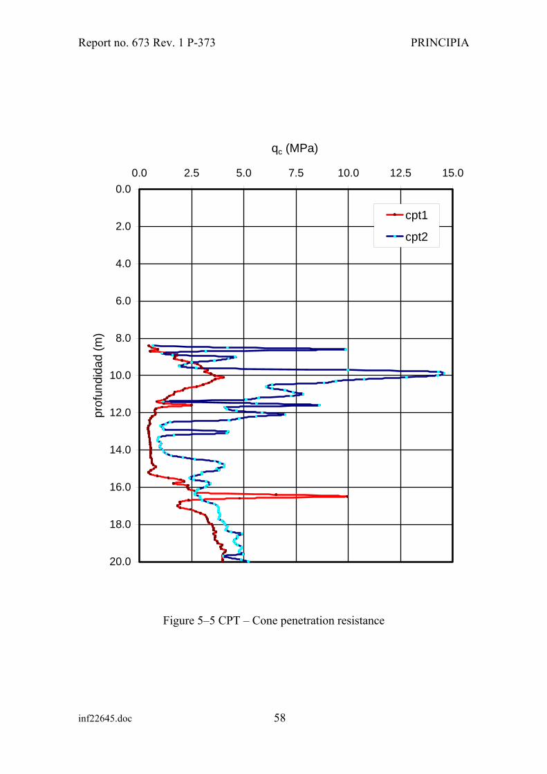
The CPT results, used for the evaluation of the liquefaction potential in Layer 4, are presented in Figures 5–5 and 5–6.

The CRR values corresponding to the (N1)60 data in Table 5–4 are presented in Table 5–5. Values of (N1)60 greater than 30 indicate that the soil is unable to liquefy, hence no value of CRR is quoted in such cases. inf22645.doc 51


inf22645.doc 52

Boreholes Lower bound Average Upper

bound

1-4 0.18 0.48 - 5-8 - - -

1-8 0.32 - -

Table 5–5 Lower, average and upper values of CRR

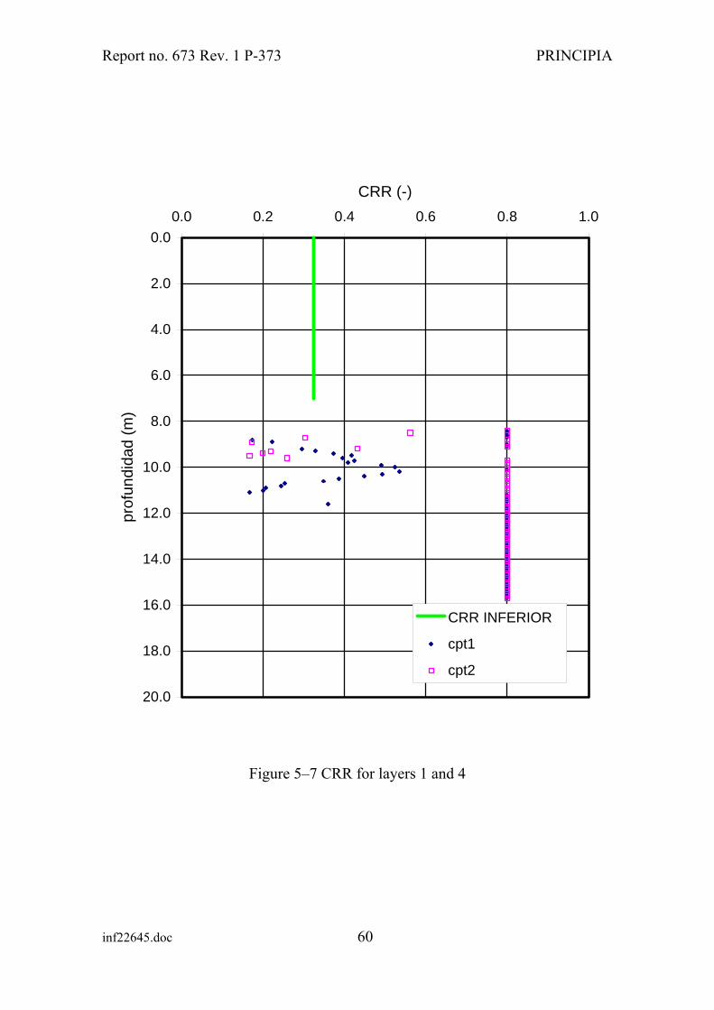
Figure 5–7 presents the lower bound of CRR (the only one numerically quantifiable) when considering all BHs (1 to 8) and the CRR resulting from the CPT data. When deriving the CRR from the CPT results, the nonliquefiable points have been given an arbitrary value of 0.8. This has no physical meaning, but serves to indicate that the majority of the CPT points predict that no liquefaction is possible.

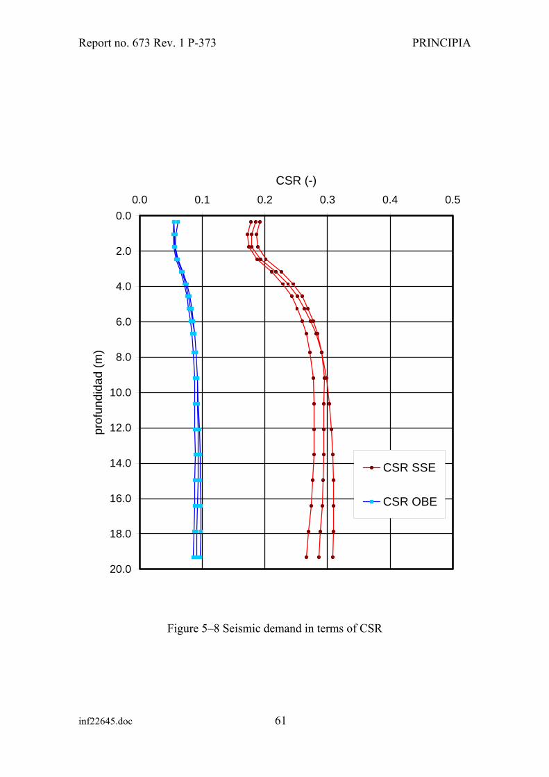
Figure 5–8 presents the seismic demand induced by each of the three earthquakes presented in section 4.3 in terms of CSR as explained at the beginning of this section.

Comparing the seismic demand and the soil capacity (Figure 5–9) it can be seen that the SSE demand in general is lower than the soil capacity. The capacity presented for Layer 1 corresponds to the lower bound when considering BH 1 to 8 (Table 5–5). The average and upper bounds correspond to nonliquefiable situations so they do not have representation in Figure 5–9.

However, if one considers only the CRR values derived from the boreholes under Tank 1 (BH 1 to 4), the SSE demand curve falls between the average and the lower bound (see Table 5–5 and Figure 5–9). The minimum CRR needed for avoiding liquefaction under the SSE is 0.3, which corresponds to a value of (N1)60 of 22.

Table 5–6 shows the percentile fractions that correspond to each set of boreholes, taking into account the distribution of the data at those boreholes. Figure 5–10 shows the lower, average and upper values for (N1)60 under tank 1, together with the one required in order to produce a CRR value greater than the seismic demand.


inf22645.doc 53

Boreholes percentile for (N1)60 = 22

1-4 33 5-8 2

1-8 15

Table 5–6 Percentile fractions of (N1)60 data below 22

In summary, if all the data are taken together, including both tanks, the possibility of liquefaction would have to be ruled out: the lower bound of the resistance (mean minus one standard deviation) is greater than the SSE demands.

However, if the data are considered independently for both tanks, the data at the tank no. 1 location no longer fulfils that condition. The mean resistance still exceeds the demands, but the lower bound of the resistance (mean minus one standard deviation) is lower than the SSE demands. The percentage of data indicating resistances below the demands is about 33%. In this situation, liquefaction cannot be completely discarded and some attention should be paid to that problem.


0.0

5.0

10.0

15.0

20.0

25.0

30.0

1.0E-04 1.0E-03 1.0E-02 1.0E-01 1.0E+00

γeff (%)

ξ (%

)

0.0

0.2

0.4

0.6

0.8

1.0

1.0E-04 1.0E-03 1.0E-02 1.0E-01 1.0E+00

γeff (%)

G/G

0 (-)

Figure 5–1 Damping and normalised G modulus vs effective strain

inf22645.doc 54


Figure 5–2 Liquefaction resistance for sands - SPT

inf22645.doc 55


Figure 5–3 Liquefaction resistance for sands - CPT

inf22645.doc 56


0.0

2.0

4.0

6.0

8.0

10.0

12.0

14.0

16.0

18.0

20.0

0 10 20 30 40 50 60 70 80 90 100

(N1)60

Dep

th (m

)

BH1 BH2 BH3 BH4

BH5 BH6 BH7 BH8

Figure 5–4 Corrected values (N1)60

inf22645.doc 57


0.0

2.0

4.0

6.0

8.0

10.0

12.0

14.0

16.0

18.0

20.0

0.0 2.5 5.0 7.5 10.0 12.5 15.0

qc (MPa)

prof

undi

dad

(m)

cpt1

cpt2

Figure 5–5 CPT – Cone penetration resistance

inf22645.doc 58


0.0

2.0

4.0

6.0

8.0

10.0

12.0

14.0

16.0

18.0

20.0

0.0 0.1 0.1 0.2 0.2 0

fs (MPa)

prof

undi

dad

(m)

.3

cpt1

cpt2

Figure 5–6 CPT – Sleeve resistance

inf22645.doc 59


0.0

2.0

4.0

6.0

8.0

10.0

12.0

14.0

16.0

18.0

20.0

0.0 0.2 0.4 0.6 0.8 1.0

CRR (-)

prof

undi

dad

(m)

CRR INFERIOR

cpt1

cpt2

Figure 5–7 CRR for layers 1 and 4

inf22645.doc 60


0.0

2.0

4.0

6.0

8.0

10.0

12.0

14.0

16.0

18.0

20.0

0.0 0.1 0.2 0.3 0.4 0.5

CSR (-)

prof

undi

dad

(m)

CSR SSE

CSR OBE

Figure 5–8 Seismic demand in terms of CSR

inf22645.doc 61


0.0

2.0

4.0

6.0

8.0

10.0

12.0

14.0

16.0

18.0

20.0

0.0 0.1 0.2 0.3 0.4 0.5 0.6 0.7 0.8 0.9 1.0

CSR (-) , CRR (-)

prof

undi

dad

(m)

CSR SSECRR INFERIOR - CPTCRR - cpt1CRR - cpt2

Figure 5–9 Comparison of demand (CSR) and resistance (CRR)

inf22645.doc 62


0.0

2.0

4.0

6.0

8.0

10.0

12.0

14.0

16.0

18.0

20.0

0 10 20 30 40 50 60 70 80 90 100

(N1)60

Dep

th (m

)

BH1 BH2 BH3 BH4

BH5 BH6 BH7 BH8

(N1)60 = 22 CRR = 0.3

Figure 5–10 (N1)60 values under Tank 1 compared with requirement

inf22645.doc 63


inf22645.doc 64

6. CONCLUSIONS

An evaluation of the seismic hazard has been conducted for the site of the new LNG plant in Taranto (Italy). The evaluation was carried out using modern zoneless procedures, which do not rely on the construction of seismogenetic provinces of uniform generating capacity. The methodology employed is solidly based from a theoretical standpoint and has been applied by Principia in evaluations of the seismic hazard at all LNG sites in Spain and some abroad.

The studies performed lead to a number of conclusions and recommendations, which are summarily listed below:

a) It is recommended that the following values be adopted for the peak horizontal ground acceleration: 0.29g for the SSE and 0.09g for the OBE. The corresponding values for the vertical motions are 0.21g for the SSE and 0.065g for the OBE.

b) Consistent with the provisions of the Italian norm OPCM (2003), site specific design spectra have been developed for both the SSE and the OBE motions. The recommended spectra are those presented in Figure 4–3 for the horizontal motions and Figure 4–4 for the vertical motions.

c) It is recommended that the following accelerograms be adopted for design: those in Figures 4–5 and 4–6 for the horizontal and vertical SSE motions, respectively, and those in Figures 4–7 and 4–8 for the horizontal and vertical OBE motions, respectively. The durations of the accelerograms are 25 s for both the SSE and the OBE, as a consequence of the requirements of the Italian norm.

d) The hazard curve obtained appears to be fairly stable under reasonable changes in the variable parameters, in particular the power-law exponent n of the kernel function. This strengthens the reliability of the design accelerations obtained.

e) It is recommended that strain-compatible soil properties be used in the evaluation of soil-structure interaction effects. The recommended


inf22645.doc 65

equivalent properties are given in Table 5–2 for the OBE and in Table 5–3 for the SSE.

f) Seismically triggered liquefaction is not considered possible under tank 2. Under tank 1, although the mean values again indicate that liquefaction would not occur, the margin does not appear to be adequate: some 33% of the data are consistent with the occurrence of liquefaction under the SSE loads. As a consequence, it is recommended that this problem be studied in more detail by the EPC contractor in order to ensure a proper performance of the tank’s foundation under the loads.


inf22645.doc 66

Appendix I. References


inf22645.doc 67

ASCE – American Society of Civil Engineers (1999) “Standard 4-98. Seismic Analysis of Safety-Related Nuclear Structures and Commentary”.

CEN – European Committee for Standardization (1994) “Eurocode 8: Design Provisions for Earthquake Resistance of Structures”, Experimental European Norm ENV 1998-1-1, October.

CEN – European Committee for Standardization (1997) “Installation and Equipment for Liquefied Natural Gas. Design of Onshore Installations”, European Standard EN 1473.

Cornell, C.A. (1968) “Engineering Seismic Risk Analysis”, Bulletin of the Seismological Society of America, Vol. 58, pp. 1583-1606.

Crespo, M.J. and Martí, J. (2002) “The Use of a Zoneless Method in Four LNG Sites in Spain”, 12th European Conference on Earthquake Engineering, London, September.

Dobry, R., Idriss, I.M. and Ng, E. (1978) “Duration Characteristic of Horizontal Components of Strong Motion Earthquake Records”, Bulletin of the Seismological Society of America, no. 68, pp. 1487-1520.

Esteva, L. and Rosenblueth, E. (1964) “Espectros de Temblores a Distancias Moderadas y Grandes”, Bulletin of the Mexican Society of Seismic Engineering, no. 2, pp. 1-18.

Gasparini, D. (1975) “SIMQKE. A Program for Artificial Motion Generation”, Department of Civil Engineering, Massachusetts Institute of Technology.

GNDT – Gruppo Nazionale per la Difensa dai Terremoti (2005) Webpage: http://emidius.mi.ingv.it/NT/CONSNT.html

Housner, G.W. (1965) “Measures of Severity of Earthquake Ground Shaking”, U.S. National Conference on Earthquake Engineering, Ann Harbor, MI.

INGV–CNT – Instituto Nazionale di Geofisica e Vulcanologia – Centro Nazionale Terremoti (2005) Webpage: ftp://ftp.ingv.it/bollet.

Kaul, K.M. (1978) "Spectrum Consistent Time History Generation", ASCE Journal of the Engineering Mechanics Division, Vol. 104, pp. 781-788.

http://emidius.mi.ingv.it/NT/CONSNT.html

ftp://ftp.ingv.it/bollet


inf22645.doc 68

Medea (2004) “Terminale di Ricezione e Rigassificazione Gas Naturale Liquefatto (GNL). Taranto (Italy). Studio Geologico Preliminare”, Doc. no. 03255-CIV-R-0-003, 24 June.

NFPA – National Fire Protection Association (2001) “NFPA 59-A. Production, Storage and Handling of Liquefied Natural Gas”, Maryland.

OPCM – Ordinanza del Presidente del Consiglio dei Ministri (2003) "Primi Elementi in Materia di Criteri Generali per la Classificazione Sismica del Territorio Nazionale e di Normative Tecniche per le Construzioni in Zona Sismica", Ordinanza n. 3274, 20 March.

Principia (2005) “LNG Plant at Taranto (Italy). Summary of Seismic Hazard Evaluation”, Report no. 674, 19 January.

Sabetta, F. and Pugliese, A. (1987) “Attenuation Law of Peak Horizontal Acceleration and Velocity from Italian Strong-Motion Records”, Bulletin of the Seismological Society of America, Vol. 77, no. 5, October, pp. 1491-1513.

Sabetta, F. and Pugliese, A. (1996) “Estimation of the Response Spectra and Simulation of Nonstationary Earthquake Ground Motions”, Bulletin of the Seismological Society of America, Vol. 86, no. 2, April, pp. 337-352.

Soil (2005) “Italia-Taranto. LNG Terminal. Onshore Terminal and Power Plant”, Final Geotechnical Report to Gas Natural no. 0797-X-TA-RE-002-A-11, 15 February.

Trifunac, M.D. and Brady, A.G. (1975) “A Study on the Duration of Strong Ground Motion”, Bulletin of the Seismological Society of America, no. 65, pp. 581-626.

Valensise, G., Amato, A., Montone, P. and Pantosti, D. (2003) “Earthquakes in Italy: Past, Present and Future”, Episodes, no. 26, 245-249.

Woo, G. (1987) “POSTQUAKE. A Program to Generate Artificial Time Histories Matching Specified Seismic Response Spectra. User’s Guide”, Principia Mechanica Ltd.

Woo, G. (1995) “A Comparative Assessment of Zoneless Models of Seismic


inf22645.doc 69

Hazard”, 5th International Conference on Seismic Zonation, Vol. I.

Woo, G. (1996a) “Kernel Estimation Methods for Seismic Hazard Area Modelling”, Bulletin of the Seismological Society of America, Vol. 86, No. 2, April, pp. 353-362.

Woo, G. (1996b) “Seismic Hazard Program: KERFRACT”, Program Documentation.


inf22645.doc 70

Appendix II. The computer program KERFRACT


inf22645.doc 71

SEISMIC HAZARD PROGRAM KERFRACT

Program Documentation Written by Dr. Gordon Woo

July 1996

1. INTRODUCTION

This documentation is prepared to explain the methodology and usage of the seismic hazard program: KERFRACT which has been written by the author with the aim of making seismic hazard computation more scientific and data-intensive, and reducing the recourse to expert judgement. To many seismologists, the standard Cornell-McGuire procedure for seismic hazard analysis, based on Euclidean zonation, is unnecessarily subjective and ad hoc. Few seismologists have been motivated to transform this standard data-reductive methodology, which was formulated to be computationally efficient 25 years ago, when computing power was still a scarce resource: about 100,000 times as expensive as it is now.

In an article in Terra Nova,Vol.6, the author (1994) originally called attention to some of the fundamental problems with conventional seismic zonation procedures. An outline of a computational approach which circumvents these problems is presented by the author in the Proceedings of the 5th International Conference on Seismic Zonation, Vol.I, (1995), and a more detailed description is published in the Bulletin of the Seismological Society of America (1996).

The essential observation underlying the new approach is the recognition that the geometry of earthquake epicentres hardly ever satisfies the constraints of spatial uniformity, as presumed by the standard Euclidean zonation method, but rather has a far richer, more structured, fractal characterisation. In order to represent this fractal geometry, a seismic source model is most conveniently constructed from the spatial pattern of earthquake epicentres, drawn both from the historical catalogue of earthquakes, and available geological information on neotectonic fault movements. The spatio-temporal distribution of earthquake epicentres


inf22645.doc 72

constitutes an interchangeable currency by which geological data can be converted (through deformation/moment relations) into an equivalent seismological form.

The existing seismological and geological databases, however large and complete, can never provide a full blueprint for future activity. Apart from the inevitable errors in earthquake magnitudes and epicentres, nonlinear dynamical effects on the seismogenic system will cause perturbations in the size and location of future events. These recording errors and irreducible dynamical perturbations require a smoothing operation to be performed on the data, such as can be implemented using statistical kernel techniques. The need for this type of smoothing to be consistent with the fractal geometry of earthquakes, has suggested the name of the seismic hazard program: KERFRACT.

2. PROGRAM ROUTINES

The Program KERGRID is written in FORTRAN, and consists of a main routine, and three subroutines EXCEED, AKER and GAUSS. Compared with zonation software, the program structure is simpler, and the coding shorter, although the demands on computer cpu time are much greater, because many more degrees of freedom in earthquake generation are represented. In order to achieve maximum quality of hazard resolution, the program has been set up to be site-specific, rather than to calculate hazard for a set of sites in a single run. Even for neighbouring sites, minor adjustments in hazard input may be warranted by geological data etc. It is intended that the program should be re-run for each different site. Compared with multiple site analysis in a single run, the benefit of greater accuracy should outweigh the additional computing cost.

The main routine reads in the site Latitude/Longitude coordinates; the kernel parameters; the hazard ground motion values; ground motion attenuation coefficients; regional earthquake depth distribution; earthquake epicentres and magnitudes, with corresponding standard deviations of uncertainties.

The core of the routine is the calculation of activity rate density fields, covering a dense square grid of sites spanning the region around the designated site of interest. The activity rate density fields are magnitude-dependent, and are determined for all magnitudes ranging upwards from the threshold of engineering interest, which is here taken to be 4.0.


inf22645.doc 73

In ascertaining the contribution of each catalogued event to a particular activity rate density field, the estimated event magnitude is smeared over a Normal distribution of values, with the prescribed standard deviation of magnitude error, and the estimated event location is smeared over a bivariate Normal distribution of values, with the standard deviation of location error.

Every event is associated with an ‘effective’ historical threshold date for its observability. The return period for the event is then obtained by subtraction of this historical date from the present date (i.e. 1996). The historical threshold date is qualified as ‘effective’ to allow for the partial observability of the event before the threshold date, and the partial unobservability of the event after it. The formal definition of the return period for a given catalogued event is 100 times the sum of the event detection probabilities in all centuries up to the present.

The characteristic of epicentres to be distributed fractally is represented by the dynamical smearing of the epentre over distance. This smoothing is performed via the Fortran Function AKER (see next section).

By summing over all catalogued events, the cumulative activity rate density is computed for each magnitude ranging from the minimum magnitude of engineering interest, (here taken to be 4.0), up to the highest value represented in the catalogue. For each event, the cumulative activity rate density is updated at each location on the regional grid. Apart from historical earthquakes, the catalogue can be supplemented by events inferred from neotectonic data, and from microtremor data. Neotectonic evidence may, for example, suggest the occurrence of earthquakes with a magnitude range beyond that of the historical catalogue.

Allowance can be made, within KERFRACT, for earthquakes occurring of size up to the regional maximum credible magnitude. A feature of the main routine is that it also includes a facility to superpose a grid of events of higher magnitude, with an activity rate density chosen to be consistent with the broad regional observational data on extreme earthquakes.

2.1 SUBROUTINE EXCEED

For a specified magnitude and for a set of ground motion levels, this routine evaluates the contribution of each grid location to the expected annual number of


inf22645.doc 74

exceedances of ground motion at the designated site. By summing over all regional grid locations, and looping over a weighted regional earthquake depth distribution, the expected annual number of exceedances of ground motion is calculated for the site in question. Assuming that such exceedances are Poisson-distributed, the annual probability of exceedance of ground motion is calculated.

The depth distribution can be made magnitude-dependent, and region-specific, if sufficient quality and quantity of depth observations exist to warrant this refinement.

2.2 FUNCTION AKER

The Function AKER defines the Kernel smoothing function. The free parameters are the power law index PL ( > 1 ), and the bandwidth function H(M) in the formula:

K (M, x ) = [ (n - 1)/Β ] H(M)-2 [1 + r2/H(M)2]-n

The scaling formula for H(M) is set at: c exp(dM)

n is typically in the range from 1.5 to 2.0

The bandwidth parameters a and b may be estimated by regression analysis of the dataset of separation distances of events of varying magnitude. For UK, c = 0.044; d = 1.55.

The above expression for the Kernel function is isotropic, i.e. the smoothing is independent of direction. This is satisfactory in regions where no particular association is discernible between earthquake locations and geological structure. However, in areas where epicentres form identifiable lineaments, some directionality in smoothing may be desirable.

Under these circumstances, an appropriate anisotropic Kernel is used. This has the form:

K (M, x ) = [ (n - 1)/ Β] H(M)-2 N {1 + cos2 Ν} [ 1 + r2/H(M)2]-n

where the normalization factor N = 1/(1 + ∗/2)]


inf22645.doc 75

In this expression, Ν is the angle subtended at x between the intersection of the fault plane with the Earth's surface and the epicentre location. ∗ is a parameter which modulates the degree of anisotropy; a zero value indicates isotropy and a value of 10 indicates significant anisotropy. With the normalization factor above, Ν lies between 0 and 2Β. For each event which requires directionally smoothing, values of ∗ and Ν need to be input.

2.3 FUNCTION GAUSS

The Function GAUSS is a standard mathematical routine which computes the cumulative probability of exceedance of a number of standard deviations for the Normal distribution.

3. PROGRAM INPUT

There are two individual input files for KERFRACT. These are called kfin.d; qkcatin.d;

KFIN.D

The first file kfin.d contains the following lines:

Title card:

Site Latitude and Longitude:

Kernel fractal scaling index : n

Kernel bandwidth parameters: c, d in the expression c exp(dM)

Epicentral error sampling flag: 0 (no sampling, i.e. no allowance for epicentral error), 1 (3 samples of Latitude and 3 of Longitude); 2 (5 samples of Latitude and 5 of Longitude)

Number of grid blocks: spanning a square area around the site.

Grid mesh dimension (kms): i.e. the size of each grid block.


inf22645.doc 76

Number of ground motion values:

Ground motion values: which should be input in increasing order.

Annual exceedance probabilities: for which ground motion values are to be computed.

Attenuation coefficients: as in the formula:

Ln A = C1 + C2*M + C4*R + C3*Ln{R + C5*Exp(C6*M)}

together with the linear regression standard deviation.

Number of depths and values (kms): appropriate for the regional earthquake depth distribution around the site.

In principle, this depth distribution could be made magnitude-dependent; this would require a programming adjustment.

Weights of the selected depth values;

Background seismicity magnitudes: generally covering the range from the highest catalogued magnitude to the maximum credible magnitude, although lower magnitude values may be included to allow for missing events in areas of poor event detectibility.

Frequencies/sq.km./year: based on seismicity statistics for a large seismotectonic region around the site.

QKCATIN.D

The second input file qkcatin.d contains a regional listing of catalogued earthquakes. If the threshold magnitude of practical engineering interest is Mmin, (typically 4.0), then, allowing for magnitude underestimates of events nominally somewhat less than this, the catalogue should include all events of magnitude Mmin - 0.5.

In areas of poor event detectability, (e.g. offshore or deserted areas), where


inf22645.doc 77

magnitude 4 or 5 events have been historically unobservable, some enhancement to the catalogue may be necessary. This is because the instrumentally recorded events of magnitude 4 or 5 may provide too sparse a picture of the potential historical frequency of such events. In this circumstance, qkcatin.d should be supplemented by hypothetical epicentres of magnitude 4 and 5 events, extrapolated from the catalogue of recently recorded events of magnitude 3. The return period of these hypothesized events may be estimated using a local b-value.

A further supplement to qkcatin.d is the addition of synthesized events corresponding to neotectonic information on regional active faulting. Where fault activity is only partially revealed by historical seismic activity, it may represented by a set of synthesized earthquake epicentres with magnitudes and return periods consistent with fault dating measurements and other geological information.

For each event, the following line of input information is required in qkcatin.d:

QKE(I,1) The recorded Latitude of the event

QKE(I,2) The recorded Longitude of the event

ERR(I,1) The standard deviation of the uncertainty in the estimate of epicentre location (kms) [This is the distance discrepancy between the estimated and true epicentres; the discrepancy is assumed to be isotropic]

QKE(I,3) The estimated magnitude of the event

ERR(I,2) The standard deviation of the uncertainty in the estimate of magnitude

IYR(I) The effective historical threshold date for observation of the event (the number of years since this date yields the effective period during which the event would most likely have been detected)

Each event is associated with two parameters which relate to the directionality of seismicity around the event epicentre.


inf22645.doc 78

DL(I) The first parameter is a measure of the strength of the directionality over isotropy; a value of zero implies isotropy, and a value of 10 or more implies significant anisotropy.

TH(I) The second parameter is the angle indicating the direction of an active lineament including the event epicentre. (Such a lineament may be a specific geological structure, or an alignment of earthquake epicentres). The convention for defining the orientation of the lineament is that this angle is measured anti-clockwise from due East. Thus a lineament oriented due East would be associated with a zero angle, and a lineament oriented due West would be associated with an angle of 180 degrees.

4. COMPUTATIONAL ISSUES

The computational demands of KERFRACT are quite high, especially if the catalogue is extensive. To avoid unnecessary use of computer time, events further than 1000 kms from the site are filtered out from consideration.

In summing the hazard contribution associated with different event magnitudes, an increment of 0.1 has been taken.

Error sampling of alternative epicentral values is computer-intensive, so a flag has been included in the input file to allow this sampling to be switched off (0); to be reasonably varied (1); and to be quite dense (2). The intermediate option is generally recommended as a practical compromise.

Other input parameters which affect the speed of computation are identified as follows:

NGRID The number of grid locations spanning the region of interest

GMESH The size of the grid mesh (kms)

These parameters can be adjusted through sensitivity analysis to determine the minimum configuration needed to obtain stable and robust results. A value of GMESH of about 2kms, or perhaps higher, may afford sufficient resolution. Depending on the ground motion frequency of interest, the overall grid span NGRID*GMESH may vary from 200kms to 500kms.

Documents

Informe no. 673 (Gas Natural): LNG Tank at Taranto (Italy