energies

Article

Influence of Various Irradiance Models and TheirCombination on Simulation Results ofPhotovoltaic Systems

Martin Hofmann 1,2,* ID and Gunther Seckmeyer 2 ID

1 Valentin Software GmbH, Stralauer Platz 34, 10243 Berlin, Germany2 Institute for Meteorology and Climatology, Leibniz Universität Hannover, Herrenhäuser Straße 2,

30419 Hannover, Germany; seckmeyer@muk.uni-hannover.de* Correspondence: martin.hofmann@valentin-software.com; Tel.: +49-30-588-4390

Academic Editor: Senthilarasu SundaramReceived: 10 August 2017; Accepted: 31 August 2017; Published: 26 September 2017

Abstract: We analyze the output of various state-of-the-art irradiance models for photovoltaic systems.The models include two sun position algorithms, three types of input data time series, nine diffusefraction models and five transposition models (for tilted surfaces), resulting in 270 different modelchains for the photovoltaic (PV) system simulation. These model chains are applied to 30 locationsworldwide and three different module tracking types, totaling in 24,300 simulations. We showthat the simulated PV yearly energy output varies between −5% and +8% for fixed mounted PVmodules and between −26% and +14% for modules with two-axis tracking. Model quality variesstrongly between locations; sun position algorithms have negligible influence on the simulationresults; diffuse fraction models add a lot of variability; and transposition models feature the strongestinfluence on the simulation results. To highlight the importance of irradiance with high temporalresolution, we present an analysis of the influence of input temporal resolution and simulationmodels on the inverter clipping losses at varying PV system sizing factors for Lindenberg, Germany.Irradiance in one-minute resolution is essential for accurately calculating inverter clipping losses.

Keywords: photovoltaics; simulation; irradiation; BSRN; diffuse; diffuse fraction; irradiance; model;transposition; high resolution; tilted; inclined

1. Introduction

Irradiance models are among the most important elements of the complex model chain forsimulations of photovoltaic systems. In an ideal case, the irradiance incident on the module plane ismeasured beforehand in-situ in high resolution, so that this time series can directly be used as an inputfor the electrical PV simulation. In standard use cases however, only the time series of the globalhorizontal irradiance in one-hour resolution at the nearest location and the location coordinates areavailable as input for time-step simulations. The models have to deliver estimates for the sun position,for the diffuse fraction of the horizontal irradiance and, most importantly, for the global irradiance onthe plane of the module.

The output of the irradiance processor model chain, the global irradiance on the tilted planeof the PV module, is the most important input parameter for the subsequent model chain that isresponsible for the electrical simulation of the modules, as the output current of any PV cell hasan approximately linear dependency from the incident irradiance, while the output voltage showsa dependency that resembles logarithmic functions. Hence, the output power of PV modules isalmost linearly dependent on the irradiance at moderate to high values, which implies a nearly linear

Energies 2017, 10, 1495; doi:10.3390/en10101495 www.mdpi.com/journal/energies

Energies 2017, 10, 1495 2 of 24

dependency of the yearly PV energy yield on the irradiation—as the integral of the irradiance overtime—on the module surface.

In this study, we want to focus on the irradiance model chain as a whole and systematicallyanalyze the interplay of the different models and their influence on the global tilted irradiance (GTI)and the PV energy as the outputs of the model chain. We use high quality global horizontal irradiance(GHI) measurement data from the Baseline Surface Radiation Network (BSRN) [1] of 30 locationsworldwide to estimate the model quality under various conditions. By altering the model chain,we combine all selected models of one category with the all models of the other categories, which leadsto a considerable amount of simulations. With this analysis, we are able to answer questions aboutthe importance of choosing the right sun position algorithm, the required temporal resolution orthe best model for the diffuse fraction. Additionally, we can make statements about the variability ofthe simulation results under given conditions.

2. Methodology

2.1. Input Data

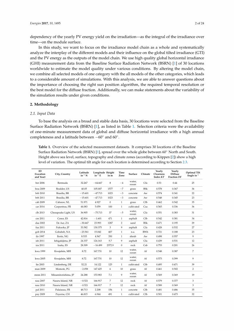
To base the analysis on a broad and stable data basis, 30 locations were selected from the BaselineSurface Radiation Network (BSRN) [1], as listed in Table 1. Selection criteria were the availabilityof one-minute measurement data of global and diffuse horizontal irradiance with a high annualcompleteness and a latitude between −60 and 60.

Table 1. Overview of the selected measurement datasets. It comprises 30 locations of the BaselineSurface Radiation Network (BSRN) [1], spread over the whole globe between 60 North and South.Height above sea level, surface, topography and climate zones (according to Köppen [2]) show a highlevel of variation. The optimal tilt angle for each location is determined according to Section 2.3.

ID(Locationand Year)

City, Country Latitudein N

Longitudein E

Heightin m

TimeZone Surface Climate

YearlyClearnessIndex KT

YearlyDiffuse

Fraction DF

Optimal TiltAngle in

ber 2006 Bermuda 32.267 −64.667 8 −4 water,ocean Cfa 0.53 0.44 25

bou 2009 Boulder, US 40.05 105.007 1577 −7 grass BSk 0.578 0.367 36

brb 2010 Brasilia, BR −15.601 −47.713 1023 −3 concrete Aw 0.574 0.341 22

brb 2011 Brasilia, BR −15.601 −47.713 1023 −3 concrete Aw 0.548 0.345 23

cab 2009 Cabauw, NL 51.971 4.927 0 1 grass Cfb 0.462 0.542 35

car 2014 Carpentras, FR 44.083 5.059 100 1 cultivated Csa 0.565 0.336 36

clh 2013 Chesapeake Light, US 36.905 −75.713 37 −5 water,ocean Cfa 0.551 0.383 31

cnr 2011 Cener, ES 42.816 −1.601 471 1 asphalt Cfb 0.542 0.381 34

daa 2002 De Aar, ZA −30.667 23.993 1287 2 sand BSk 0.671 0.195 29

fua 2011 Fukuoka, JP 33.582 130.375 3 9 asphalt Cfa 0.428 0.532 27

gob 2014 Gobabeb, NA −23.561 15.042 407 1 n.a. BWh 0.721 0.188 23

ilo 1997 Ilorin, NG 8.533 4.567 350 1 shrub Aw 0.498 0.557 9

ish 2011 Ishigakijima, JP 24.337 124.163 5.7 9 asphalt Cfa 0.439 0.531 12

iza 2011 Izaña, ES 28.309 −16.499 2372.9 0 rock Csb 0.753 0.201 26

kwa 1999 Kwajalein, MH 8.72 167.731 10 12 water,ocean Af 0.548 0.387 7

kwa 2005 Kwajalein, MH 8.72 167.731 10 12 water,ocean Af 0.573 0.399 9

lin 2003 Lindenberg, DE 52.21 14.122 125 1 cultivated Cfb 0.495 0.471 39

man 2009 Momote, PG −2.058 147.425 6 10 grass Af 0.461 0.502 2

mnm 2011 Minamitorishima, JP 24.288 153.983 7.1 9 water,ocean Af 0.569 0.369 19

nau 2007 Nauru Island, NR −0.521 166.917 7 12 rock Af 0.579 0.377 3

nau 2010 Nauru Island, NR −0.521 166.917 7 12 rock Af 0.589 0.369 3

pal 2011 Palaiseau, FR 48.713 2.208 156 1 concrete Cfb 0.481 0.486 35

pay 2009 Payerne, CH 46.815 6.944 491 1 cultivated Cfb 0.501 0.473 32

Energies 2017, 10, 1495 3 of 24

Table 1. Cont.

ID(Locationand Year)

City, Country Latitudein N

Longitudein E

Heightin m

TimeZone Surface Climate

YearlyClearnessIndex KT

YearlyDiffuse

Fraction DF

Optimal TiltAngle in

reg 2011 Regina, CA 50.205 −104.713 578 −6 cultivated BSk 0.593 0.401 41

sap 2011 Sapporo, JP 43.06 141.328 17.2 9 asphalt Dfb 0.442 0.549 35

sbo 2009 Sede Boqer, IL 30.905 34.782 500 2 desertrock Cwb 0.665 0.261 27

sov 2001 Solar Village, SA 24.91 46.41 650 3 desert,sand BWh 0.705 0.278 23

tat 2006 Tateno, JP 36.05 140.133 25 9 grass Cfa 0.413 0.558 35

tor 2006 (*) Toravere, EE 58.254 26.462 70 2 grass Dfb 0.481 0.446 41

xia 2006 (*) Xianghe, CN 39.754 116.962 32 8 desert,rock Dwa 0.468 0.576 34

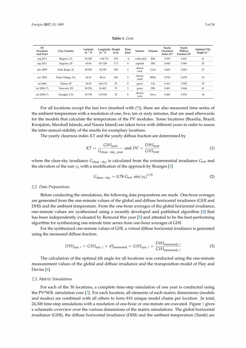
For all locations except the last two (marked with (*)), there are also measured time series ofthe ambient temperature with a resolution of one, five, ten or sixty minutes, that are used afterwardsfor the models that calculate the temperature of the PV modules. Some locations (Brasilia, Brazil;Kwajalein, Marshall Islands; and Nauru Island) are taken twice with different years in order to assessthe inter-annual stability of the results for exemplary locations.

The yearly clearness index KT and the yearly diffuse fraction are determined by

KT =GHIyear

Gclear−sky, yearand DF =

DHIyear

GHIyear(1)

where the clear-sky irradiance Gclear−sky is calculated from the extraterrestrial irradiance Gext andthe elevation of the sun γs with a modification of the approach by Bourges [3]

Gclear−sky = 0.78 Gext sin(γS)1.15 (2)

2.2. Data Preparations

Before conducting the simulations, the following data preparations are made. One-hour averagesare generated from the one-minute values of the global and diffuse horizontal irradiance (GHI andDHI) and the ambient temperature. From the one-hour averages of the global horizontal irradiance,one-minute values are synthesized using a recently developed and published algorithm [4] thathas been independently evaluated by Remund this year [5] and attested to be the best-performingalgorithm for synthesizing one-minute time series from one-hour averages of GHI.

For the synthesized one-minute values of GHI, a virtual diffuse horizontal irradiance is generatedusing the measured diffuse fraction:

DHIsyn, i = GHIsyn, i ∗ d fmeasured = GHIsyn, i ∗DHImeasured, i

GHImeasured, i(3)

The calculation of the optimal tilt angle for all locations was conducted using the one-minutemeasurement values of the global and diffuse irradiance and the transposition model of Hay andDavies [6].

2.3. Matrix Simulations

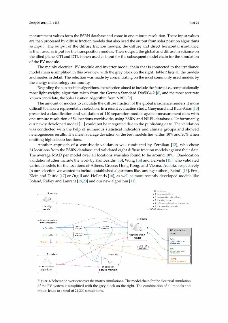
For each of the 30 locations, a complete time-step simulation of one year is conducted usingthe PV*SOL simulation core [7]. For each location, all elements of each matrix dimensions (modelsand modes) are combined with all others to form 810 unique model chains per location. In total,24,300 time-step simulations with a resolution of one-hour or one-minute are executed. Figure 1 givesa schematic overview over the various dimensions of the matrix simulations. The global horizontalirradiance (GHI), the diffuse horizontal irradiance (DHI) and the ambient temperature (Tamb) are

Energies 2017, 10, 1495 4 of 24

measurement values form the BSRN database and come in one-minute resolution. These input valuesare then processed by diffuse fraction models that also need the output from solar position algorithmsas input. The output of the diffuse fraction models, the diffuse and direct horizontal irradiance,is then used as input for the transposition models. Their output, the global and diffuse irradiance onthe tilted plane, GTI and DTI, is then used as input for the subsequent model chain for the simulationof the PV module.

The mainly electrical PV module and inverter model chain that is connected to the irradiancemodel chain is simplified in this overview with the grey block on the right. Table 2 lists all the modelsand modes in detail. The selection was made by concentrating on the most commonly used models bythe energy meteorology community.

Regarding the sun position algorithms, the selection aimed to include the fastest, i.e., computationallymost light-weight, algorithm taken from the German Standard Din5034-2 [8], and the most accurateknown candidate, the Solar Position Algorithm from NREL [9].

The amount of models to calculate the diffuse fraction of the global irradiance renders it moredifficult to make a representative selection. In a recent evaluation study, Gueymard and Ruiz-Arias [10]presented a classification and validation of 140 separation models against measurement data withone-minute resolution of 54 locations worldwide, using BSRN and NREL databases. Unfortunately,our newly developed model [11] could not be integrated due to the publishing date. The validationwas conducted with the help of numerous statistical indicators and climate groups and showedheterogeneous results. The mean average deviation of the best models lies within 10% and 20% whenomitting high albedo locations.

Another approach of a worldwide validation was conducted by Zernikau [12], who chose24 locations from the BSRN database and validated eight diffuse fraction models against their data.The average MAD per model over all locations was also found to lie around 10%. One-locationvalidation studies include the work by Kambezidis [13], Wong [14] and Dervishi [15], who validatedvarious models for the locations of Athens, Greece; Hong Kong; and Vienna, Austria, respectively.In our selection we wanted to include established algorithms like, amongst others, Reindl [16], Erbs,Klein and Duffie [17] or Orgill and Hollands [18], as well as more recently developed models likeBoland, Ridley and Laurent [19,20] and our new algorithm [11].

Energies 2017, 10, 1495 4 of 23

and modes in detail. The selection was made by concentrating on the most commonly used models by the energy meteorology community.

Regarding the sun position algorithms, the selection aimed to include the fastest, i.e., computationally most light-weight, algorithm taken from the German Standard Din5034-2 [8], and the most accurate known candidate, the Solar Position Algorithm from NREL [9].

The amount of models to calculate the diffuse fraction of the global irradiance renders it more difficult to make a representative selection. In a recent evaluation study, Gueymard and Ruiz-Arias [10] presented a classification and validation of 140 separation models against measurement data with one-minute resolution of 54 locations worldwide, using BSRN and NREL databases. Unfortunately, our newly developed model [11] could not be integrated due to the publishing date. The validation was conducted with the help of numerous statistical indicators and climate groups and showed heterogeneous results. The mean average deviation of the best models lies within 10% and 20% when omitting high albedo locations.

Another approach of a worldwide validation was conducted by Zernikau [12], who chose 24 locations from the BSRN database and validated eight diffuse fraction models against their data. The average MAD per model over all locations was also found to lie around 10%. One-location validation studies include the work by Kambezidis [13], Wong [14] and Dervishi [15], who validated various models for the locations of Athens, Greece; Hong Kong; and Vienna, Austria, respectively. In our selection we wanted to include established algorithms like, amongst others, Reindl [16], Erbs, Klein and Duffie [17] or Orgill and Hollands [18], as well as more recently developed models like Boland, Ridley and Laurent [19,20] and our new algorithm [11].

Figure 1. Schematic overview over the matrix simulations. The model chain for the electrical simulation of the PV system is simplified with the grey block on the right. The combination of all models and inputs leads to a total of 24,300 simulations.

Table 2. Overview over the dimensions of the matrix simulation.

Dimension Models/Modes AmountLocations See Table 1 30

Input data/time resolution • 1-min measurement values

3 • 1-min synthesized values [4] • 1-h averaged values

Sun position • Din5034-2 [8]

2 • NREL SPA [9]

Figure 1. Schematic overview over the matrix simulations. The model chain for the electrical simulationof the PV system is simplified with the grey block on the right. The combination of all models andinputs leads to a total of 24,300 simulations.

Energies 2017, 10, 1495 5 of 24

Table 2. Overview over the dimensions of the matrix simulation.

Dimension Models/Modes Amount

Locations See Table 1 30

Input data/time resolution• 1-min measurement values• 1-min synthesized values [4]• 1-h averaged values

3

Sun position • Din5034-2 [8]• NREL SPA [9]

2

Tracking mode

• Fixed tilt at 40, facing south on northern hemisphere,north on southern hemisphere

• Optimal tilt angle for each location, see Table 1• Two-axis tracking with 180 East-West rotation limit

3

Diffuse fraction

• Measurement values• Models

# Reindl reduced [16]# Boland, Ridley and Laurent (BRL) [19]# Boland, Ridley and Laurent 2010 (BRL 2010) [20]# Erbs, Klein and Duffie (EKD) [17]# Orgill and Hollands (OH) [18]# Skartveit [21]# Perez and Ineichen (PI) [22]# Hofmann [11]

9

Transposition models (irradianceon module plane)

• Liu and Jordan [23]• Hay and Davies [6]• Klucher [24]• Perez [25]• Reindl [26]

5

Total 24,300

A multitude of transposition models to calculate the irradiance on tilted surfaces has beendeveloped in the past 60 years, and many validation studies have been presented. The first modelto name is the isotropic approach of Liu and Jordan [23], other well-known and widely used modelsare Hay and Davies [6], Klucher [24], Perez [25] and Reindl [26]. These five models constitute ourchoice for the matrix simulations. There exist a lot more transposition models, where the approachesby Temps and Coulson [27], Muneer [28], Olmo [29], Gueymard [30] and Badescu [31] are probablythe most well-known and validated except the models listed above.

Notable recent validation studies include the work by Yang [32], who lists and compares 26 modelsagainst one-minute measurement data from four locations with two to eight sensor orientations each,see values in brackets: Eugene, OR, USA (3); Oldenburg, Germany (2); Singapore (8); and Golden,CO, USA (5); the normalized MBD was found to lie between −11% and +12% for tilt angles up to 45

and between −45% and +20% for vertical surfaces. Another comprehensive contribution is made byIneichen [33], who validates eight models against one-minute and one-hour data of two locations andthe studies of Loutzenhiser [34], Gueymard [35], Demain [36] and Gulin [37], who compare seven to14 models against the measurement data of one location. In these studies, measurement data were fromGeneva and Duebendorf, Switzerland; Denver and Golden, CO, USA; Uccle, Belgium; and Zagreb, HR.

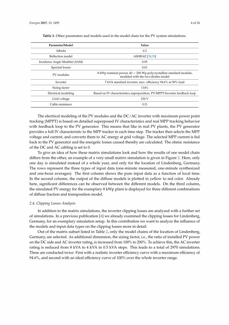
Other parameters and models used in the simulation of the PV system are listed in Table 3.These values and models represent the default setting in most simulation software like PV*SOL.The albedo value of 0.2 represents a ground reflectance of, e.g., sand, grass or asphalt. The reflectionmodel and the Incidence Angle Modifier (IAM) define how much irradiance is reflected on the glasssurface of the PV module. The spectral losses consider the fact that the spectral distribution ofthe irradiance might not be equal to the AM1.5 solar spectrum on which the PV modules are tested.

Energies 2017, 10, 1495 6 of 24

Table 3. Other parameters and models used in the model chain for the PV system simulations.

Parameter/Model Value

Albedo 0.2

Reflection model ASHRAE [38,39]

Incidence Angle Modifier (IAM) 0.95

Spectral losses 0.01

PV modules 8 kWp nominal power, 40 × 200 Wp polycrystalline standard module,modeled with the two-diodes model

Inverter 7 kVA standard inverter, max. efficiency 94.6% at 50% load

Sizing factor 114%

Electrical modeling Based on IV characteristics superposition, PV-MPPT-Inverter feedback loop

Grid voltage 230 V

Cable resistance 0 Ω

The electrical modeling of the PV modules and the DC/AC inverter with maximum power pointtracking (MPPT) is based on detailed superposed IV characteristics and real MPP tracking behaviorwith feedback loop to the PV generator. This means that like in real PV plants, the PV generatorprovides a full IV characteristic to the MPP tracker in each time step. The tracker then selects the MPPvoltage and current, and converts them to AC energy at grid voltage. The selected MPP current is fedback to the PV generator and the energetic losses caused thereby are calculated. The ohmic resistanceof the DC and AC cabling is set to 0.

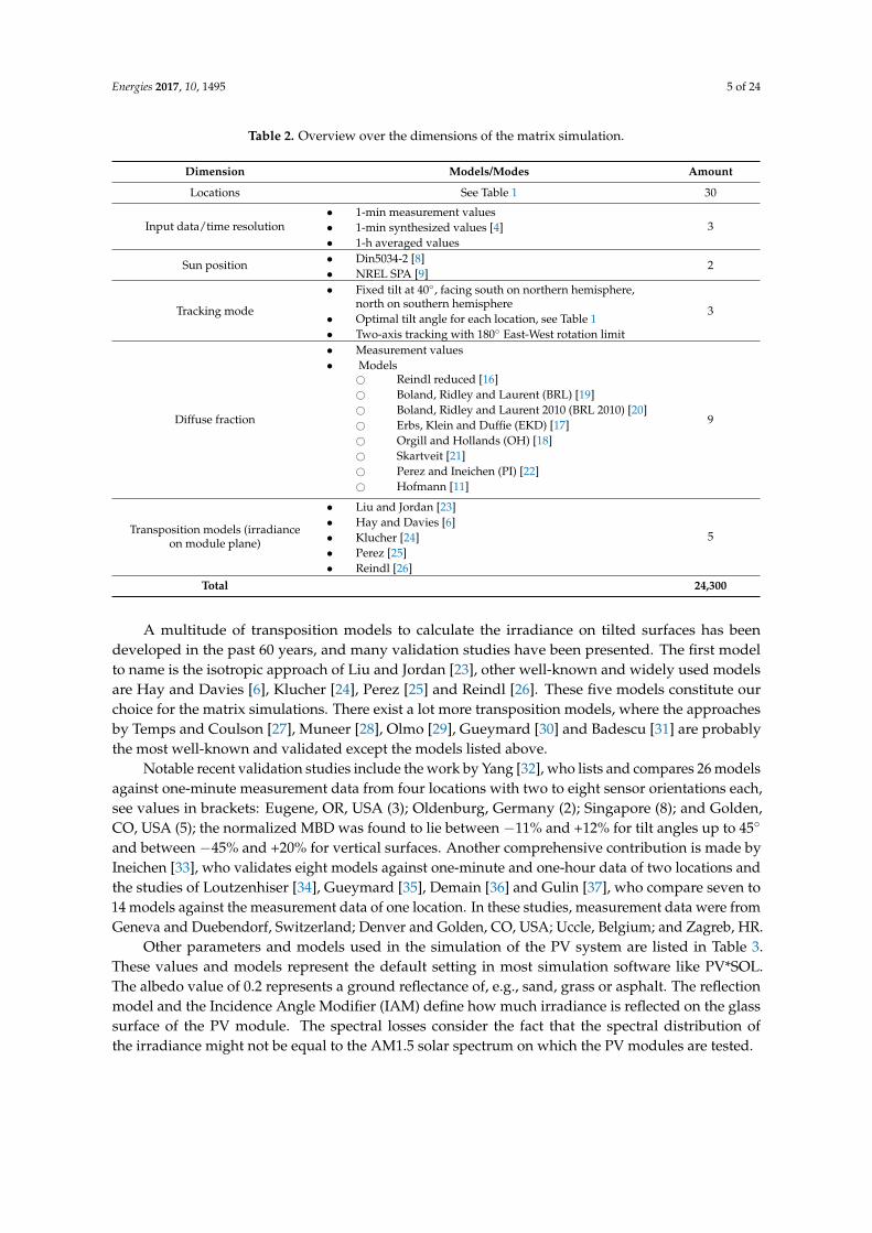
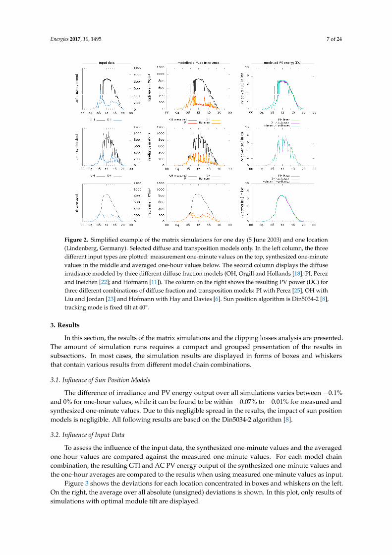
To give an idea of how these matrix simulations look and how the results of one model chaindiffers from the other, an example of a very small matrix simulation is given in Figure 2. Here, onlyone day is simulated instead of a whole year, and only for the location of Lindenberg, Germany.The rows represent the three types of input data (one-minute measured, one-minute synthesizedand one-hour averages). The first column shows the pure input data as a function of local time.In the second column, the output of the diffuse models is plotted in yellow to red color. Alreadyhere, significant differences can be observed between the different models. On the third column,the simulated PV energy for the exemplary 8 kWp plant is displayed for three different combinationsof diffuse fraction and transposition model.

2.4. Clipping Losses Analysis

In addition to the matrix simulations, the inverter clipping losses are analyzed with a further setof simulations. In a previous publication [4] we already examined the clipping losses for Lindenberg,Germany, for an exemplary simulation setup. In this contribution we want to analyze the influence ofthe models and input data types on the clipping losses more in detail.

Out of the matrix subset listed in Table 2, only the model chains of the location of Lindenberg,Germany, are selected. As additional dimension, the sizing factor, i.e., the ratio of installed PV poweron the DC side and AC inverter rating, is increased from 100% to 200%. To achieve this, the AC inverterrating is reduced from 8 kVA to 4 kVA in 0.5 kVA steps. This leads to a total of 2970 simulations.These are conducted twice: First with a realistic inverter efficiency curve with a maximum efficiency of94.6%, and second with an ideal efficiency curve of 100% over the whole inverter range.

Energies 2017, 10, 1495 7 of 24

Energies 2017, 10, 1495 6 of 23

Table 3. Other parameters and models used in the model chain for the PV system simulations.

Parameter/Model ValueAlbedo 0.2

Reflection model ASHRAE [38,39] Incidence Angle Modifier

(IAM) 0.95

Spectral losses 0.01

PV modules 8 kWp nominal power, 40 × 200 Wp polycrystalline standard module, modeled with the

two-diodes model Inverter 7 kVA standard inverter, max. efficiency 94.6% at 50% load

Sizing factor 114% Electrical modeling Based on IV characteristics superposition, PV-MPPT-Inverter feedback loop

Grid voltage 230 V Cable resistance 0 Ω

To give an idea of how these matrix simulations look and how the results of one model chain differs from the other, an example of a very small matrix simulation is given in Figure 2. Here, only one day is simulated instead of a whole year, and only for the location of Lindenberg, Germany. The rows represent the three types of input data (one-minute measured, one-minute synthesized and one-hour averages). The first column shows the pure input data as a function of local time. In the second column, the output of the diffuse models is plotted in yellow to red color. Already here, significant differences can be observed between the different models. On the third column, the simulated PV energy for the exemplary 8 kWp plant is displayed for three different combinations of diffuse fraction and transposition model.

Figure 2. Simplified example of the matrix simulations for one day (5 June 2003) and one location (Lindenberg, Germany). Selected diffuse and transposition models only. In the left column, the three different input types are plotted: measurement one-minute values on the top, synthesized one-minute values in the middle and averaged one-hour values below. The second column displays the diffuse irradiance modeled by three different diffuse fraction models (OH, Orgill and Hollands [18]; PI, Perez and Ineichen [22]; and Hofmann [11]). The column on the right shows the resulting PV power (DC) for three different combinations of diffuse fraction and transposition models: PI with Perez [25], OH with Liu and Jordan [23] and Hofmann with Hay and Davies [6]. Sun position algorithm is Din5034-2 [8], tracking mode is fixed tilt at 40°.

Figure 2. Simplified example of the matrix simulations for one day (5 June 2003) and one location(Lindenberg, Germany). Selected diffuse and transposition models only. In the left column, the threedifferent input types are plotted: measurement one-minute values on the top, synthesized one-minutevalues in the middle and averaged one-hour values below. The second column displays the diffuseirradiance modeled by three different diffuse fraction models (OH, Orgill and Hollands [18]; PI, Perezand Ineichen [22]; and Hofmann [11]). The column on the right shows the resulting PV power (DC) forthree different combinations of diffuse fraction and transposition models: PI with Perez [25], OH withLiu and Jordan [23] and Hofmann with Hay and Davies [6]. Sun position algorithm is Din5034-2 [8],tracking mode is fixed tilt at 40.

3. Results

In this section, the results of the matrix simulations and the clipping losses analysis are presented.The amount of simulation runs requires a compact and grouped presentation of the results insubsections. In most cases, the simulation results are displayed in forms of boxes and whiskersthat contain various results from different model chain combinations.

3.1. Influence of Sun Position Models

The difference of irradiance and PV energy output over all simulations varies between −0.1%and 0% for one-hour values, while it can be found to be within −0.07% to −0.01% for measured andsynthesized one-minute values. Due to this negligible spread in the results, the impact of sun positionmodels is negligible. All following results are based on the Din5034-2 algorithm [8].

3.2. Influence of Input Data

To assess the influence of the input data, the synthesized one-minute values and the averagedone-hour values are compared against the measured one-minute values. For each model chaincombination, the resulting GTI and AC PV energy output of the synthesized one-minute values andthe one-hour averages are compared to the results when using measured one-minute values as input.

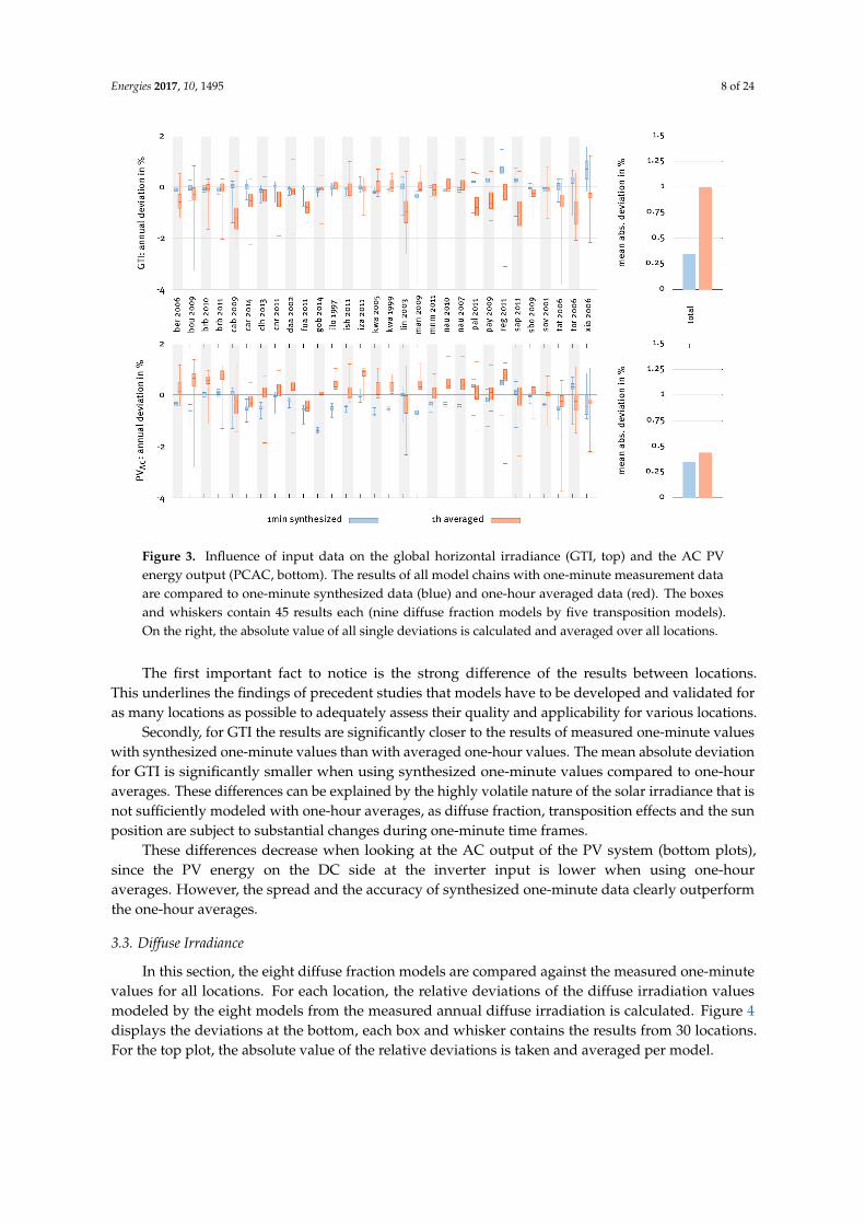
Figure 3 shows the deviations for each location concentrated in boxes and whiskers on the left.On the right, the average over all absolute (unsigned) deviations is shown. In this plot, only results ofsimulations with optimal module tilt are displayed.

Energies 2017, 10, 1495 8 of 24Energies 2017, 10, 1495 8 of 23

Figure 3. Influence of input data on the global horizontal irradiance (GTI, top) and the AC PV energy output (PCAC, bottom). The results of all model chains with one-minute measurement data are compared to one-minute synthesized data (blue) and one-hour averaged data (red). The boxes and whiskers contain 45 results each (nine diffuse fraction models by five transposition models). On the right, the absolute value of all single deviations is calculated and averaged over all locations.

These differences decrease when looking at the AC output of the PV system (bottom plots), since the PV energy on the DC side at the inverter input is lower when using one-hour averages. However, the spread and the accuracy of synthesized one-minute data clearly outperform the one-hour averages.

3.3. Diffuse Irradiance

In this section, the eight diffuse fraction models are compared against the measured one-minute values for all locations. For each location, the relative deviations of the diffuse irradiation values modeled by the eight models from the measured annual diffuse irradiation is calculated. Figure 4 displays the deviations at the bottom, each box and whisker contains the results from 30 locations. For the top plot, the absolute value of the relative deviations is taken and averaged per model.

As recently shown in the presentation of our new diffuse fraction model [11], our approach (Hofmann) is capable of producing mean absolute deviations (MAD) of around 6% for one-minute values (grey). The other models produce MAD of 10% to 16%, which also corresponds to the findings in previous analyses. For synthesized one-minute values the results are similar, the Hofmann model produced the smallest deviation slightly elevated MAD. For one-hour averages, the Hofmann model still produces the smallest MAD, but other models are also featuring MAD of less than 10%.

The bottom part of the plot reveals deeper insight in the quality of the diffuse fraction models and the spread of their results. While, e.g., the “Reindl red.” and the “BRL” model lead to similar MAD in the top plot, the boxes and whiskers in the bottom plot show significant differences. The spread is higher for the “Reindl red.” model, from −12% to +50% but the box remains between −9% and +8% with the median at 0%, i.e., 50% of all simulation results lead to deviations of less than ±10%. The “BRL” model however has its median at −13% with the box only covering the range from −16% to −6% which reveals a systematic underestimation of the diffuse fraction by this model.

Figure 3. Influence of input data on the global horizontal irradiance (GTI, top) and the AC PVenergy output (PCAC, bottom). The results of all model chains with one-minute measurement dataare compared to one-minute synthesized data (blue) and one-hour averaged data (red). The boxesand whiskers contain 45 results each (nine diffuse fraction models by five transposition models).On the right, the absolute value of all single deviations is calculated and averaged over all locations.

The first important fact to notice is the strong difference of the results between locations.This underlines the findings of precedent studies that models have to be developed and validated foras many locations as possible to adequately assess their quality and applicability for various locations.

Secondly, for GTI the results are significantly closer to the results of measured one-minute valueswith synthesized one-minute values than with averaged one-hour values. The mean absolute deviationfor GTI is significantly smaller when using synthesized one-minute values compared to one-houraverages. These differences can be explained by the highly volatile nature of the solar irradiance that isnot sufficiently modeled with one-hour averages, as diffuse fraction, transposition effects and the sunposition are subject to substantial changes during one-minute time frames.

These differences decrease when looking at the AC output of the PV system (bottom plots),since the PV energy on the DC side at the inverter input is lower when using one-houraverages. However, the spread and the accuracy of synthesized one-minute data clearly outperformthe one-hour averages.

3.3. Diffuse Irradiance

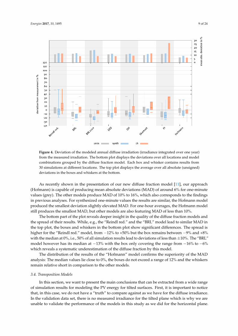
In this section, the eight diffuse fraction models are compared against the measured one-minutevalues for all locations. For each location, the relative deviations of the diffuse irradiation valuesmodeled by the eight models from the measured annual diffuse irradiation is calculated. Figure 4displays the deviations at the bottom, each box and whisker contains the results from 30 locations.For the top plot, the absolute value of the relative deviations is taken and averaged per model.

Energies 2017, 10, 1495 9 of 24Energies 2017, 10, 1495 9 of 23

Figure 4. Deviation of the modeled annual diffuse irradiation (irradiance integrated over one year) from the measured irradiation. The bottom plot displays the deviations over all locations and model combinations grouped by the diffuse fraction model. Each box and whisker contains results from 30 simulations at different locations. The top plot displays the average over all absolute (unsigned) deviations in the boxes and whiskers at the bottom.

The distribution of the results of the “Hofmann” model confirms the superiority of the MAD analysis: The median values lie close to 0%, the boxes do not exceed a range of 12% and the whiskers remain relative short in comparison to the other models.

3.4. Transposition Models

In this section, we want to present the main conclusions that can be extracted from a wide range of simulation results for modeling the PV energy for tilted surfaces. First, it is important to notice that, in this case, we do not have a “truth” to compare against as we have for the diffuse irradiance. In the validation data set, there is no measured irradiance for the tilted plane which is why we are unable to validate the performance of the models in this study as we did for the horizontal plane. However, other studies have analyzed and validated a subset of these transposition models in the past, most notably by Yang [32] and Gueymard [35], for selected locations and tilt angles.

In the absence of validation data, we focus on the analysis of the qualitative differences of the five transposition models and give an idea on their influence on PV system simulations.

In Figure 5, the annual irradiation gains for the tilted modules are plotted over the tilt angle of the module for the five analyzed transposition models. The irradiation gains were calculated with one-hour data of Berlin, Germany, from Meteonorm [40]. Significant differences in the model output can be observed throughout the tilt angle range. While the Klucher model [24] even produces irradiation gains of >0% for horizontal modules due to a term on the diffuse irradiation that is not fully dependent on the tilt angle, the isotropic model by Liu and Jordan [23] calculates the lowest irradiation gains over the whole tilt angle range. For tilt angles for over 28°, the model by Perez [25] produces the highest gains.

Figure 4. Deviation of the modeled annual diffuse irradiation (irradiance integrated over one year)from the measured irradiation. The bottom plot displays the deviations over all locations and modelcombinations grouped by the diffuse fraction model. Each box and whisker contains results from30 simulations at different locations. The top plot displays the average over all absolute (unsigned)deviations in the boxes and whiskers at the bottom.

As recently shown in the presentation of our new diffuse fraction model [11], our approach(Hofmann) is capable of producing mean absolute deviations (MAD) of around 6% for one-minutevalues (grey). The other models produce MAD of 10% to 16%, which also corresponds to the findingsin previous analyses. For synthesized one-minute values the results are similar, the Hofmann modelproduced the smallest deviation slightly elevated MAD. For one-hour averages, the Hofmann modelstill produces the smallest MAD, but other models are also featuring MAD of less than 10%.

The bottom part of the plot reveals deeper insight in the quality of the diffuse fraction models andthe spread of their results. While, e.g., the “Reindl red.” and the “BRL” model lead to similar MAD inthe top plot, the boxes and whiskers in the bottom plot show significant differences. The spread ishigher for the “Reindl red.” model, from −12% to +50% but the box remains between −9% and +8%with the median at 0%, i.e., 50% of all simulation results lead to deviations of less than ±10%. The “BRL”model however has its median at −13% with the box only covering the range from −16% to −6%which reveals a systematic underestimation of the diffuse fraction by this model.

The distribution of the results of the “Hofmann” model confirms the superiority of the MADanalysis: The median values lie close to 0%, the boxes do not exceed a range of 12% and the whiskersremain relative short in comparison to the other models.

3.4. Transposition Models

In this section, we want to present the main conclusions that can be extracted from a wide rangeof simulation results for modeling the PV energy for tilted surfaces. First, it is important to noticethat, in this case, we do not have a “truth” to compare against as we have for the diffuse irradiance.In the validation data set, there is no measured irradiance for the tilted plane which is why we areunable to validate the performance of the models in this study as we did for the horizontal plane.

Energies 2017, 10, 1495 10 of 24

However, other studies have analyzed and validated a subset of these transposition models in the past,most notably by Yang [32] and Gueymard [35], for selected locations and tilt angles.

In the absence of validation data, we focus on the analysis of the qualitative differences ofthe five transposition models and give an idea on their influence on PV system simulations.

In Figure 5, the annual irradiation gains for the tilted modules are plotted over the tilt angleof the module for the five analyzed transposition models. The irradiation gains were calculatedwith one-hour data of Berlin, Germany, from Meteonorm [40]. Significant differences in the modeloutput can be observed throughout the tilt angle range. While the Klucher model [24] even producesirradiation gains of >0% for horizontal modules due to a term on the diffuse irradiation that is not fullydependent on the tilt angle, the isotropic model by Liu and Jordan [23] calculates the lowest irradiationgains over the whole tilt angle range. For tilt angles for over 28, the model by Perez [25] producesthe highest gains.Energies 2017, 10, 1495 10 of 23

Figure 5. Annual tilt irradiation gains for various transposition models, calculated for Berlin, Germany, with one-hour climate data from Meteonorm [40]. The optimum tilt angles calculated by the models lie in the range from 31° to 38°. The Liu and Jordan model [23] produces the lowest irradiance gains while the model by Perez [25] produces the highest gains for tilt angles higher than 28°. Remarkably, the Klucher models [24] produces an irradiation gain of >0% for horizontal modules. It also produces highest gains for tilt angles up to 28°.

The calculated optimum tilt angle ranges between 31° for the Liu and Jordan model [23] (maximum tilt gain of 10%) and 38° for the Perez model [25] (maximum tilt gain of 18%). These significant differences can be observed in similar intensity over the whole tilt angle range: The irradiation loss for vertical modules (90°) ranges from −14% for the Perez model [25] to −23% for the Liu and Jordan model [23].

These results are in good agreement with the results of the reviews by Yadav [41] and Hafez [42] that also find the optimal tilt angle to vary significantly depending on the method used for determining it. The differences in energy gains presented in [41] between optimal yearly, seasonal and monthly tilt angles are found to be in the same range that is perceivable in Figures 5 and 6.

The study of Beringer [43] also compares measurements of tilt angle energy gains with modeled values for Hannover, Germany, and presents variations of the energy gain over the tilt angles that are comparable to the results presented here. The conclusion drawn in that study is fundamentally different, however, as it considers a difference of the annual PV energy yield of up to 6% as negligible.

Figure 6 displays the irradiation gains for all 30 locations over the latitude for three module mounting modes: With a fixed tilt of 40°, with a location-dependent optimum tilt (see Table 1) and with two-axis tracking. Each data point is calculated as the average of all model chains containing the respective transposition model. As expected, a clear dependency of the irradiation gains from the latitude is apparent for all three tracking modes. The longer the distance to the equator, the higher the irradiation gains will be. The small offsets to 0 for locations near the equator (man 2009 and nau 2007/2010) can be explained by reflection losses.

Figure 5. Annual tilt irradiation gains for various transposition models, calculated for Berlin, Germany,with one-hour climate data from Meteonorm [40]. The optimum tilt angles calculated by the modelslie in the range from 31 to 38. The Liu and Jordan model [23] produces the lowest irradiance gainswhile the model by Perez [25] produces the highest gains for tilt angles higher than 28. Remarkably,the Klucher models [24] produces an irradiation gain of >0% for horizontal modules. It also produceshighest gains for tilt angles up to 28.

The calculated optimum tilt angle ranges between 31 for the Liu and Jordan model [23](maximum tilt gain of 10%) and 38 for the Perez model [25] (maximum tilt gain of 18%).These significant differences can be observed in similar intensity over the whole tilt angle range:The irradiation loss for vertical modules (90) ranges from −14% for the Perez model [25] to −23% forthe Liu and Jordan model [23].

These results are in good agreement with the results of the reviews by Yadav [41] and Hafez [42]that also find the optimal tilt angle to vary significantly depending on the method used for determiningit. The differences in energy gains presented in [41] between optimal yearly, seasonal and monthly tiltangles are found to be in the same range that is perceivable in Figures 5 and 6.

Energies 2017, 10, 1495 11 of 24Energies 2017, 10, 1495 11 of 23

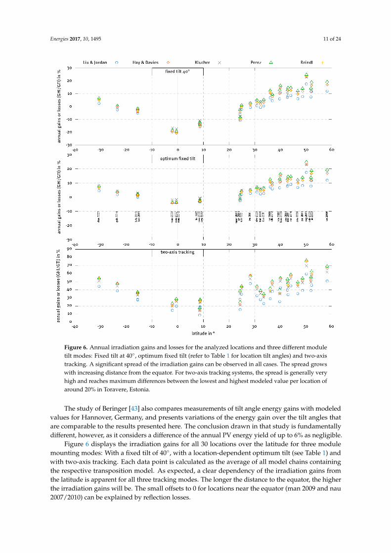
Figure 6. Annual irradiation gains and losses for the analyzed locations and three different module tilt modes: Fixed tilt at 40°, optimum fixed tilt (refer to Table 1 for location tilt angles) and two-axis tracking. A significant spread of the irradiation gains can be observed in all cases. The spread grows with increasing distance from the equator. For two-axis tracking systems, the spread is generally very high and reaches maximum differences between the lowest and highest modeled value per location of around 20% in Toravere, Estonia.

In general, a wide spread between calculated irradiation gains can be observed. The model by Liu and Jordan [23] leads to the lowest gains whereas the models by Klucher [24] and Perez [25] lead to the highest gains depending on the location and tilt mode. The maximum spread between the models is about 20% for two-axis tracking systems in Toravere, Estonia. For two-axis tracking systems in general, a spread of 10% to 15% can be observed.

3.5. Variance of Calculated PV Energy

For systems with a fixed tilt at 40° and optimum tilt the simulated PV energy varies between −5% and +8% (grey boxes and whiskers on the left and middle). For two-axis tracking systems, the results lie between −11% and +12% (left grey box and whisker). For synthesized one-minute values as input (blue), the distribution is of the same quality but shows slightly higher values. One-hour

Figure 6. Annual irradiation gains and losses for the analyzed locations and three different moduletilt modes: Fixed tilt at 40, optimum fixed tilt (refer to Table 1 for location tilt angles) and two-axistracking. A significant spread of the irradiation gains can be observed in all cases. The spread growswith increasing distance from the equator. For two-axis tracking systems, the spread is generally veryhigh and reaches maximum differences between the lowest and highest modeled value per location ofaround 20% in Toravere, Estonia.

The study of Beringer [43] also compares measurements of tilt angle energy gains with modeledvalues for Hannover, Germany, and presents variations of the energy gain over the tilt angles thatare comparable to the results presented here. The conclusion drawn in that study is fundamentallydifferent, however, as it considers a difference of the annual PV energy yield of up to 6% as negligible.

Figure 6 displays the irradiation gains for all 30 locations over the latitude for three modulemounting modes: With a fixed tilt of 40, with a location-dependent optimum tilt (see Table 1) andwith two-axis tracking. Each data point is calculated as the average of all model chains containingthe respective transposition model. As expected, a clear dependency of the irradiation gains fromthe latitude is apparent for all three tracking modes. The longer the distance to the equator, the higherthe irradiation gains will be. The small offsets to 0 for locations near the equator (man 2009 and nau2007/2010) can be explained by reflection losses.

Energies 2017, 10, 1495 12 of 24

In general, a wide spread between calculated irradiation gains can be observed. The model byLiu and Jordan [23] leads to the lowest gains whereas the models by Klucher [24] and Perez [25] lead tothe highest gains depending on the location and tilt mode. The maximum spread between the modelsis about 20% for two-axis tracking systems in Toravere, Estonia. For two-axis tracking systems ingeneral, a spread of 10% to 15% can be observed.

3.5. Variance of Calculated PV Energy

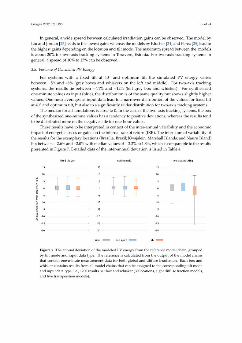
For systems with a fixed tilt at 40 and optimum tilt the simulated PV energy variesbetween −5% and +8% (grey boxes and whiskers on the left and middle). For two-axis trackingsystems, the results lie between −11% and +12% (left grey box and whisker). For synthesizedone-minute values as input (blue), the distribution is of the same quality but shows slightly highervalues. One-hour averages as input data lead to a narrower distribution of the values for fixed tiltat 40 and optimum tilt, but also to a significantly wider distribution for two-axis tracking systems.

The median for all simulations is close to 0. In the case of the two-axis tracking systems, the boxof the synthesized one-minute values has a tendency to positive deviations, whereas the results tendto be distributed more on the negative side for one-hour values.

These results have to be interpreted in context of the inter-annual variability and the economicimpact of energetic losses or gains on the internal rate of return (IRR). The inter-annual variability ofthe results for the exemplary locations (Brasilia, Brazil; Kwajalein, Marshall Islands; and Nauru Island)lies between −2.6% and +2.0% with median values of −2.2% to 1.8%, which is comparable to the resultspresented in Figure 7. Detailed data of the inter-annual deviation is listed in Table 4.

Energies 2017, 10, 1495 12 of 23

averages as input data lead to a narrower distribution of the values for fixed tilt at 40° and optimum tilt, but also to a significantly wider distribution for two-axis tracking systems.

The median for all simulations is close to 0. In the case of the two-axis tracking systems, the box of the synthesized one-minute values has a tendency to positive deviations, whereas the results tend to be distributed more on the negative side for one-hour values.

These results have to be interpreted in context of the inter-annual variability and the economic impact of energetic losses or gains on the internal rate of return (IRR). The inter-annual variability of the results for the exemplary locations (Brasilia, Brazil; Kwajalein, Marshall Islands; and Nauru Island) lies between −2.6% and +2.0% with median values of −2.2% to 1.8%, which is comparable to the results presented in Figure 7. Detailed data of the inter-annual deviation is listed in Table 4.

Figure 7. The annual deviation of the modeled PV energy from the reference model chain, grouped by tilt mode and input data type. The reference is calculated from the output of the model chains that contain one-minute measurement data for both global and diffuse irradiation. Each box and whisker contains results from all model chains that can be assigned to the corresponding tilt mode and input data type, i.e., 1200 results per box and whisker (30 locations, eight diffuse fraction models, and five transposition models).

Table 4. Inter-annual variability of the results for fixed-tilt systems for the locations of Brasilia, Brazil (BRB), Kwajalein (KWA) and Nauru Island (NAU).

Location Deviation Min Q2 Median Q3 Max

BRB (2010 and 2011) devGTI −0.0109 −0.0070 −0.0062 −0.0055 −0.0042 devPV −0.0081 −0.0055 −0.0047 −0.0041 −0.0020

KWA (1999 and 2005)

devGTI −0.0260 −0.0235 −0.0222 −0.0207 −0.0162 devPV −0.0189 −0.0164 −0.0157 −0.0148 −0.0103

NAU (2007 and 2010)

devGTI 0.0150 0.0166 0.0172 0.0176 0.0189 devPV 0.0153 0.0169 0.0175 0.0184 0.0199

For PV system simulations, three main statements can be extracted from these results:

1. Positive: For most of the combinations of models for different locations, the simulated PV energy differs only by a few percent from the reference.

2. Negative: For some combinations, however, the deviation can be as high as −5% to 8% for fixed tilt systems and up to ±12% for two-axis tracking systems.

3. Negative: There is a very high uncertainty of the model quality when using one-hour averages on two-axis tracking systems.

Figure 7. The annual deviation of the modeled PV energy from the reference model chain, groupedby tilt mode and input data type. The reference is calculated from the output of the model chainsthat contain one-minute measurement data for both global and diffuse irradiation. Each box andwhisker contains results from all model chains that can be assigned to the corresponding tilt modeand input data type, i.e., 1200 results per box and whisker (30 locations, eight diffuse fraction models,and five transposition models).

Energies 2017, 10, 1495 13 of 24

Table 4. Inter-annual variability of the results for fixed-tilt systems for the locations of Brasilia, Brazil(BRB), Kwajalein (KWA) and Nauru Island (NAU).

Location Deviation Min Q2 Median Q3 Max

BRB (2010 and 2011)devGTI −0.0109 −0.0070 −0.0062 −0.0055 −0.0042devPV −0.0081 −0.0055 −0.0047 −0.0041 −0.0020

KWA (1999 and 2005)devGTI −0.0260 −0.0235 −0.0222 −0.0207 −0.0162devPV −0.0189 −0.0164 −0.0157 −0.0148 −0.0103

NAU (2007 and 2010)devGTI 0.0150 0.0166 0.0172 0.0176 0.0189devPV 0.0153 0.0169 0.0175 0.0184 0.0199

For PV system simulations, three main statements can be extracted from these results:

1. Positive: For most of the combinations of models for different locations, the simulated PV energydiffers only by a few percent from the reference.

2. Negative: For some combinations, however, the deviation can be as high as −5% to 8% for fixedtilt systems and up to ±12% for two-axis tracking systems.

3. Negative: There is a very high uncertainty of the model quality when using one-hour averageson two-axis tracking systems.

The effect of energy losses on the IRR of a solar power investment is influenced by numerousvariables and has to be analyzed on a case-by-case basis. For a simple grid feed-in PV system in Berlin,Germany, for example, with a feed-in tariff according to the EEG 2017 [44], no loan financing andwithout the consideration of taxes, the IRR decreases by 2.5% for every energy loss of 1%. That meansthat an energy loss of 8%, which is within the scope of the variability, can lead to a reduction of the IRRof 20% and can render a PV project uneconomical.

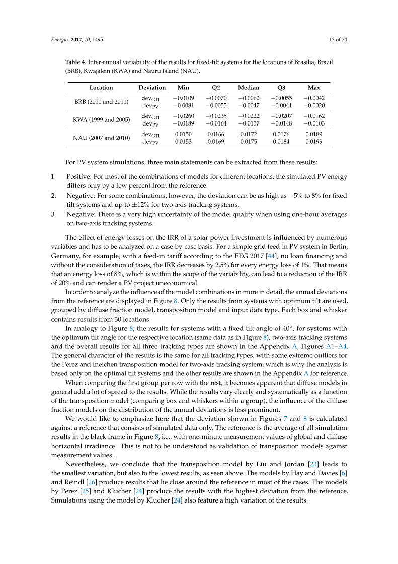
In order to analyze the influence of the model combinations in more in detail, the annual deviationsfrom the reference are displayed in Figure 8. Only the results from systems with optimum tilt are used,grouped by diffuse fraction model, transposition model and input data type. Each box and whiskercontains results from 30 locations.

In analogy to Figure 8, the results for systems with a fixed tilt angle of 40, for systems withthe optimum tilt angle for the respective location (same data as in Figure 8), two-axis tracking systemsand the overall results for all three tracking types are shown in the Appendix A, Figures A1–A4.The general character of the results is the same for all tracking types, with some extreme outliers forthe Perez and Ineichen transposition model for two-axis tracking system, which is why the analysis isbased only on the optimal tilt systems and the other results are shown in the Appendix A for reference.

When comparing the first group per row with the rest, it becomes apparent that diffuse models ingeneral add a lot of spread to the results. While the results vary clearly and systematically as a functionof the transposition model (comparing box and whiskers within a group), the influence of the diffusefraction models on the distribution of the annual deviations is less prominent.

We would like to emphasize here that the deviation shown in Figures 7 and 8 is calculatedagainst a reference that consists of simulated data only. The reference is the average of all simulationresults in the black frame in Figure 8, i.e., with one-minute measurement values of global and diffusehorizontal irradiance. This is not to be understood as validation of transposition models againstmeasurement values.

Nevertheless, we conclude that the transposition model by Liu and Jordan [23] leads tothe smallest variation, but also to the lowest results, as seen above. The models by Hay and Davies [6]and Reindl [26] produce results that lie close around the reference in most of the cases. The modelsby Perez [25] and Klucher [24] produce the results with the highest deviation from the reference.Simulations using the model by Klucher [24] also feature a high variation of the results.

Energies 2017, 10, 1495 14 of 24

Energies 2017, 10, 1495 13 of 23

The effect of energy losses on the IRR of a solar power investment is influenced by numerous variables and has to be analyzed on a case-by-case basis. For a simple grid feed-in PV system in Berlin, Germany, for example, with a feed-in tariff according to the EEG 2017 [44], no loan financing and without the consideration of taxes, the IRR decreases by 2.5% for every energy loss of 1%. That means that an energy loss of 8%, which is within the scope of the variability, can lead to a reduction of the IRR of 20% and can render a PV project uneconomical.

In order to analyze the influence of the model combinations in more in detail, the annual deviations from the reference are displayed in Figure 8. Only the results from systems with optimum tilt are used, grouped by diffuse fraction model, transposition model and input data type. Each box and whisker contains results from 30 locations.

Figure 8. The annual deviation of the modeled PV energy from the reference model chain, grouped by diffuse fraction model, transposition model and input data type. The reference is calculated from the output of the model chains that contain one-minute measurement data for both global and diffuse irradiation (black frame). Each box and whisker contains results from 30 locations. Here, only the results of the optimal tilt mode are displayed. See Appendix A Figures A1–A4 for other tilt modes and overall results.

In analogy to Figure 8, the results for systems with a fixed tilt angle of 40°, for systems with the optimum tilt angle for the respective location (same data as in Figure 8), two-axis tracking systems

Figure 8. The annual deviation of the modeled PV energy from the reference model chain, groupedby diffuse fraction model, transposition model and input data type. The reference is calculated fromthe output of the model chains that contain one-minute measurement data for both global and diffuseirradiation (black frame). Each box and whisker contains results from 30 locations. Here, only the resultsof the optimal tilt mode are displayed. See Appendix A Figures A1–A4 for other tilt modes andoverall results.

3.6. Inverter Clipping Losses

In this section, we present the results of the analysis of the inverter clipping losses for the locationof Lindenberg, Germany, 2003. As described in Section 2.4, the inverter AC rating is decreasedfrom 8 kVA to 4 kVA in steps of 0.5 kVA, which leads to sizing factors that increase from 100% to 200%.The PV plant is simulated with every combination of diffuse fraction and transposition models, and forall three types of input data: one-minute measurement, one-minute synthesized and one-hour averages.

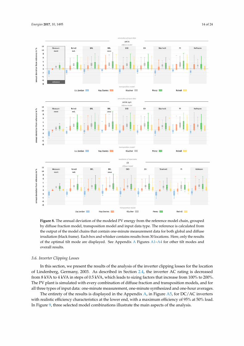
The entirety of the results is displayed in the Appendix A, in Figure A5, for DC/AC inverterswith realistic efficiency characteristics at the lower end, with a maximum efficiency of 95% at 50% load.In Figure 9, three selected model combinations illustrate the main aspects of the analysis.

Energies 2017, 10, 1495 15 of 24

Energies 2017, 10, 1495 14 of 23

and the overall results for all three tracking types are shown in the Appendix A, Figures A1–A4. The general character of the results is the same for all tracking types, with some extreme outliers for the Perez and Ineichen transposition model for two-axis tracking system, which is why the analysis is based only on the optimal tilt systems and the other results are shown in the Appendix A for reference.

When comparing the first group per row with the rest, it becomes apparent that diffuse models in general add a lot of spread to the results. While the results vary clearly and systematically as a function of the transposition model (comparing box and whiskers within a group), the influence of the diffuse fraction models on the distribution of the annual deviations is less prominent.

We would like to emphasize here that the deviation shown in Figures 7 and 8 is calculated against a reference that consists of simulated data only. The reference is the average of all simulation results in the black frame in Figure 8, i.e., with one-minute measurement values of global and diffuse horizontal irradiance. This is not to be understood as validation of transposition models against measurement values.

Nevertheless, we conclude that the transposition model by Liu and Jordan [23] leads to the smallest variation, but also to the lowest results, as seen above. The models by Hay and Davies [6] and Reindl [26] produce results that lie close around the reference in most of the cases. The models by Perez [25] and Klucher [24] produce the results with the highest deviation from the reference. Simulations using the model by Klucher [24] also feature a high variation of the results.

3.6. Inverter Clipping Losses

In this section, we present the results of the analysis of the inverter clipping losses for the location of Lindenberg, Germany, 2003. As described in Section 2.4, the inverter AC rating is decreased from 8 kVA to 4 kVA in steps of 0.5 kVA, which leads to sizing factors that increase from 100% to 200%. The PV plant is simulated with every combination of diffuse fraction and transposition models, and for all three types of input data: one-minute measurement, one-minute synthesized and one-hour averages.

The entirety of the results is displayed in the Appendix A, in Figure A5, for DC/AC inverters with realistic efficiency characteristics at the lower end, with a maximum efficiency of 95% at 50% load. In Figure 9, three selected model combinations illustrate the main aspects of the analysis.

For comparison, the results of simulations with ideal inverters are displayed in the Appendix A, Figure A6.

Figure 9. Inverter clipping losses as a function of the sizing factor of the PV plant, for one-minute measurement and synthesized data and one-hour averages. Three different combinations of diffuse fraction and transposition models as example. The clipping losses at 150% sizing factor for all model combinations are displayed in Figure 10.

In all of the analyzed cases, the clipping losses are significantly higher when using one-minute data compared to one-hour averages. When using one-hour averages as input data, the simulated clipping losses remain at 0% up until sizing factors of 120%, where one-minute data already show significant losses of 1% and more. The underestimation of the inverter clipping losses continues to

Figure 9. Inverter clipping losses as a function of the sizing factor of the PV plant, for one-minutemeasurement and synthesized data and one-hour averages. Three different combinations of diffusefraction and transposition models as example. The clipping losses at 150% sizing factor for all modelcombinations are displayed in Figure 10.

Energies 2017, 10, 1495 15 of 23

rise until around 160% sizing factor, where the simulated losses using one-minute data lie around 8%, with losses using one-hour averages at around 5%, an underestimation of over 60%.

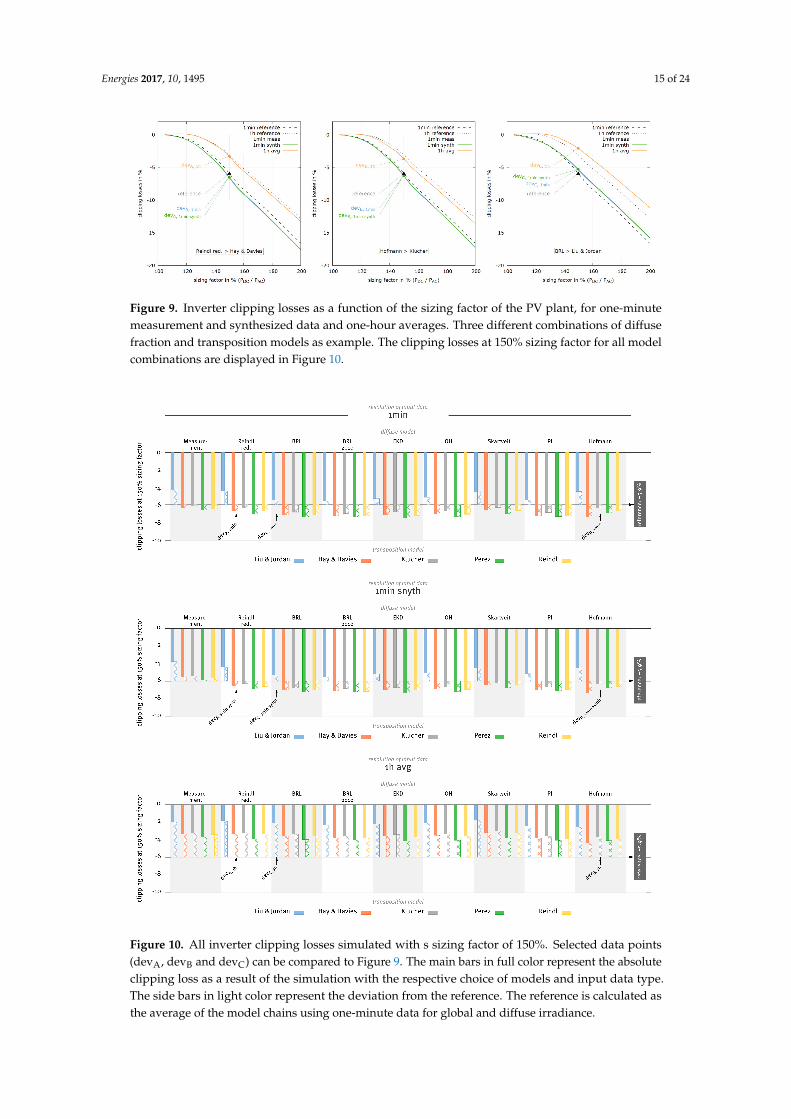
Figure 10. All inverter clipping losses simulated with s sizing factor of 150%. Selected data points (devA, devB and devC) can be compared to Figure 9. The main bars in full color represent the absolute clipping loss as a result of the simulation with the respective choice of models and input data type. The side bars in light color represent the deviation from the reference. The reference is calculated as the average of the model chains using one-minute data for global and diffuse irradiance.

The absolute value of the clipping loss also depends on the selected models for the diffuse fraction and transposition. Figure 10 displays the clipping losses for all model combination and input data types for a sizing factor of 150%. There is no significant difference in clipping losses when using synthesized one-minute data instead of measured (compare top plot against middle plot). When using one-hour averages, the clipping losses lie between 2% and 4%, while the reference calculated from one-minute data of global and diffuse irradiance lies at 5.9%.

The influence of the models for the diffuse fraction cannot be clearly answered again, as the main drivers for simulation differences remain the transposition models. Again, the model by Liu and Jordan [23] leads to underestimated clipping losses, while the model by Klucher [24] leads to the highest values in most of the cases.

Figure 10. All inverter clipping losses simulated with s sizing factor of 150%. Selected data points(devA, devB and devC) can be compared to Figure 9. The main bars in full color represent the absoluteclipping loss as a result of the simulation with the respective choice of models and input data type.The side bars in light color represent the deviation from the reference. The reference is calculated asthe average of the model chains using one-minute data for global and diffuse irradiance.

Energies 2017, 10, 1495 16 of 24

For comparison, the results of simulations with ideal inverters are displayed in the Appendix A,Figure A6.

In all of the analyzed cases, the clipping losses are significantly higher when using one-minutedata compared to one-hour averages. When using one-hour averages as input data, the simulatedclipping losses remain at 0% up until sizing factors of 120%, where one-minute data already showsignificant losses of 1% and more. The underestimation of the inverter clipping losses continues torise until around 160% sizing factor, where the simulated losses using one-minute data lie around 8%,with losses using one-hour averages at around 5%, an underestimation of over 60%.

The absolute value of the clipping loss also depends on the selected models for the diffuse fractionand transposition. Figure 10 displays the clipping losses for all model combination and input datatypes for a sizing factor of 150%. There is no significant difference in clipping losses when usingsynthesized one-minute data instead of measured (compare top plot against middle plot). When usingone-hour averages, the clipping losses lie between 2% and 4%, while the reference calculated fromone-minute data of global and diffuse irradiance lies at 5.9%.

The influence of the models for the diffuse fraction cannot be clearly answered again,as the main drivers for simulation differences remain the transposition models. Again, the modelby Liu and Jordan [23] leads to underestimated clipping losses, while the model by Klucher [24] leadsto the highest values in most of the cases.

To simulate PV plants with sizing factors of more than 110%, one-minute values are needed.This corresponds to the findings by Burger and Rüther [45] and Ransome [46]. If measured values arenot available, the use of synthetic values is highly recommended.

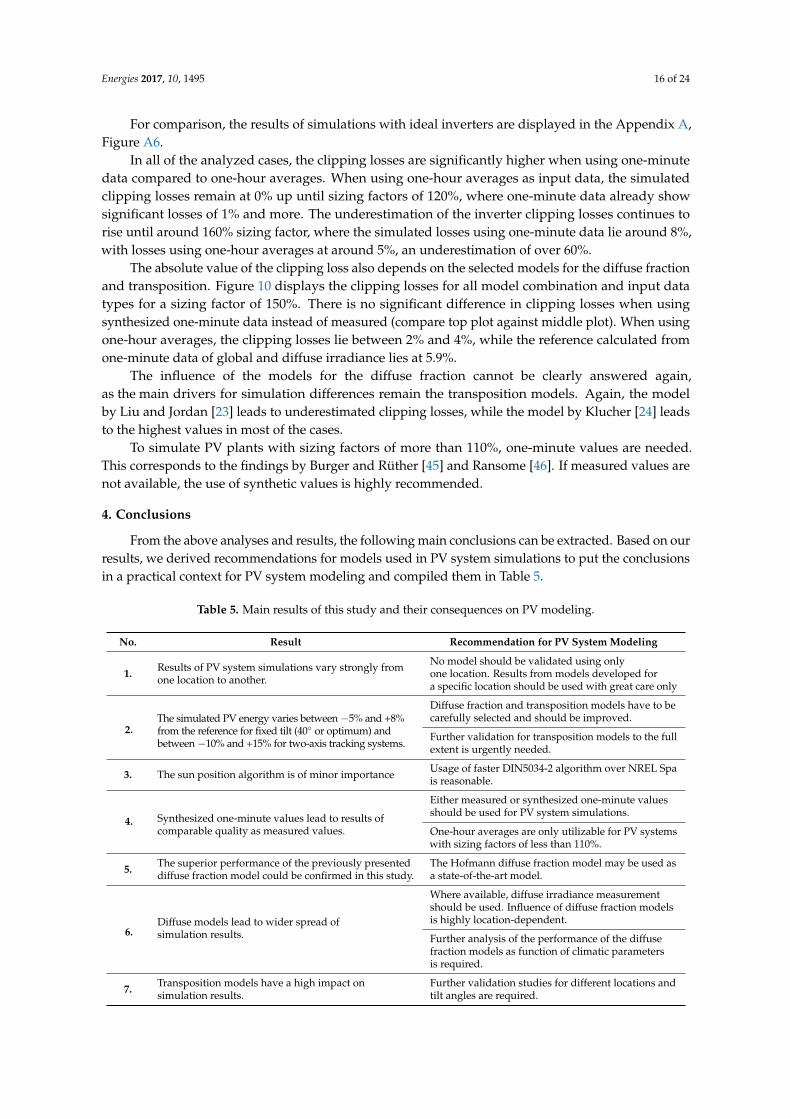
4. Conclusions

From the above analyses and results, the following main conclusions can be extracted. Based on ourresults, we derived recommendations for models used in PV system simulations to put the conclusionsin a practical context for PV system modeling and compiled them in Table 5.

Table 5. Main results of this study and their consequences on PV modeling.

No. Result Recommendation for PV System Modeling

1. Results of PV system simulations vary strongly fromone location to another.

No model should be validated using onlyone location. Results from models developed fora specific location should be used with great care only

2.The simulated PV energy varies between −5% and +8%from the reference for fixed tilt (40 or optimum) andbetween −10% and +15% for two-axis tracking systems.

Diffuse fraction and transposition models have to becarefully selected and should be improved.

Further validation for transposition models to the fullextent is urgently needed.

3. The sun position algorithm is of minor importance Usage of faster DIN5034-2 algorithm over NREL Spais reasonable.

4. Synthesized one-minute values lead to results ofcomparable quality as measured values.

Either measured or synthesized one-minute valuesshould be used for PV system simulations.

One-hour averages are only utilizable for PV systemswith sizing factors of less than 110%.

5. The superior performance of the previously presenteddiffuse fraction model could be confirmed in this study.

The Hofmann diffuse fraction model may be used asa state-of-the-art model.

6.Diffuse models lead to wider spread ofsimulation results.

Where available, diffuse irradiance measurementshould be used. Influence of diffuse fraction modelsis highly location-dependent.

Further analysis of the performance of the diffusefraction models as function of climatic parametersis required.

7. Transposition models have a high impact onsimulation results.

Further validation studies for different locations andtilt angles are required.

Energies 2017, 10, 1495 17 of 24

It should be emphasized that the present study does not reveal the impact of spectral effects,which become more important for tilted surfaces. In addition, we investigate the effect on yearlysums only. Even if this is presently the most relevant feature for PV systems, effects on the diurnalvariation will be become more important for the use of renewable energies in the future in the absenceof large and cheap energy storage systems. One aspect that deserves more attention than was possiblein the scope of this paper is the dependency of the performance of diffuse models on the climaticconditions at a location. This study also highlights the importance to intensify the effort to validatetransposition models in order to minimize the uncertainties of PV system simulations. In the absenceof globally available high-resolution measurement data of the irradiance on tilted planes, however,this task incorporates a complexity that is not to be underestimated. Future work must includethorough meta-study analyses on the topic, data collection of high quality measurement setups andintense validation.

Acknowledgments: The publication of this article was funded by the Open Access Fund of the LeibnizUniversität Hannover.

Author Contributions: Martin Hofmann designed the study, implemented the simulations, analysed the dataand edited the manuscript. Gunther Seckmeyer helped editing the manuscript.

Conflicts of Interest: The authors declare no conflict of interest.

Energies 2017, 10, 1495 18 of 24

Appendix A

Fixed 40:

Energies 2017, 10, x FOR PEER REVIEW 17 of 23

Appendix A

Fixed 40°:

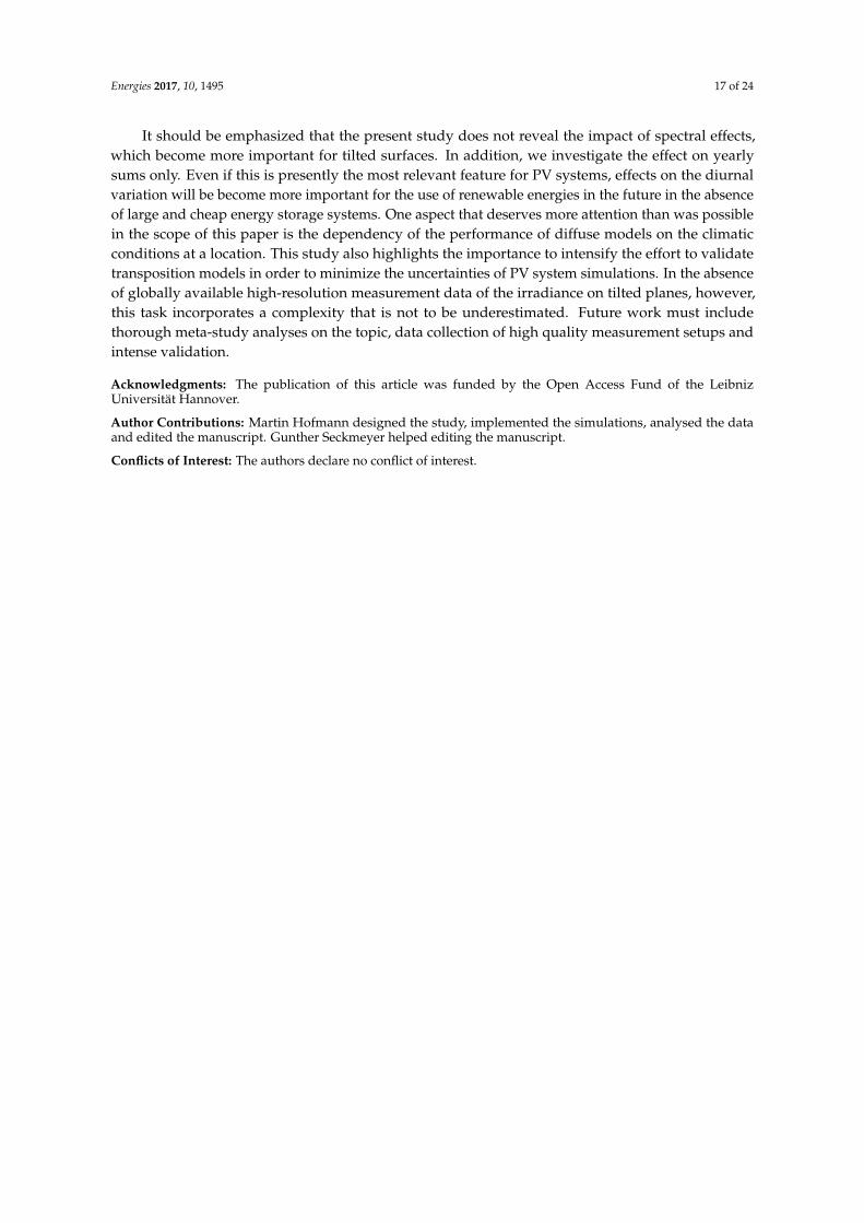
Figure A1. The annual deviation of the modeled PV energy from the reference model chain, grouped by diffuse fraction model, transposition model and input data type. The reference is calculated from the output of the model chains that contain one-minute measurement data for both global and diffuse irradiation (black frame). Each box and whisker contains results from 30 locations.

Figure A1. The annual deviation of the modeled PV energy from the reference model chain, grouped by diffuse fraction model, transposition model and input datatype. The reference is calculated from the output of the model chains that contain one-minute measurement data for both global and diffuse irradiation (black frame).Each box and whisker contains results from 30 locations.

Energies 2017, 10, 1495 19 of 24

Optimum Tilt:Energies 2017, 10, 1495 18 of 23

Optimum Tilt:

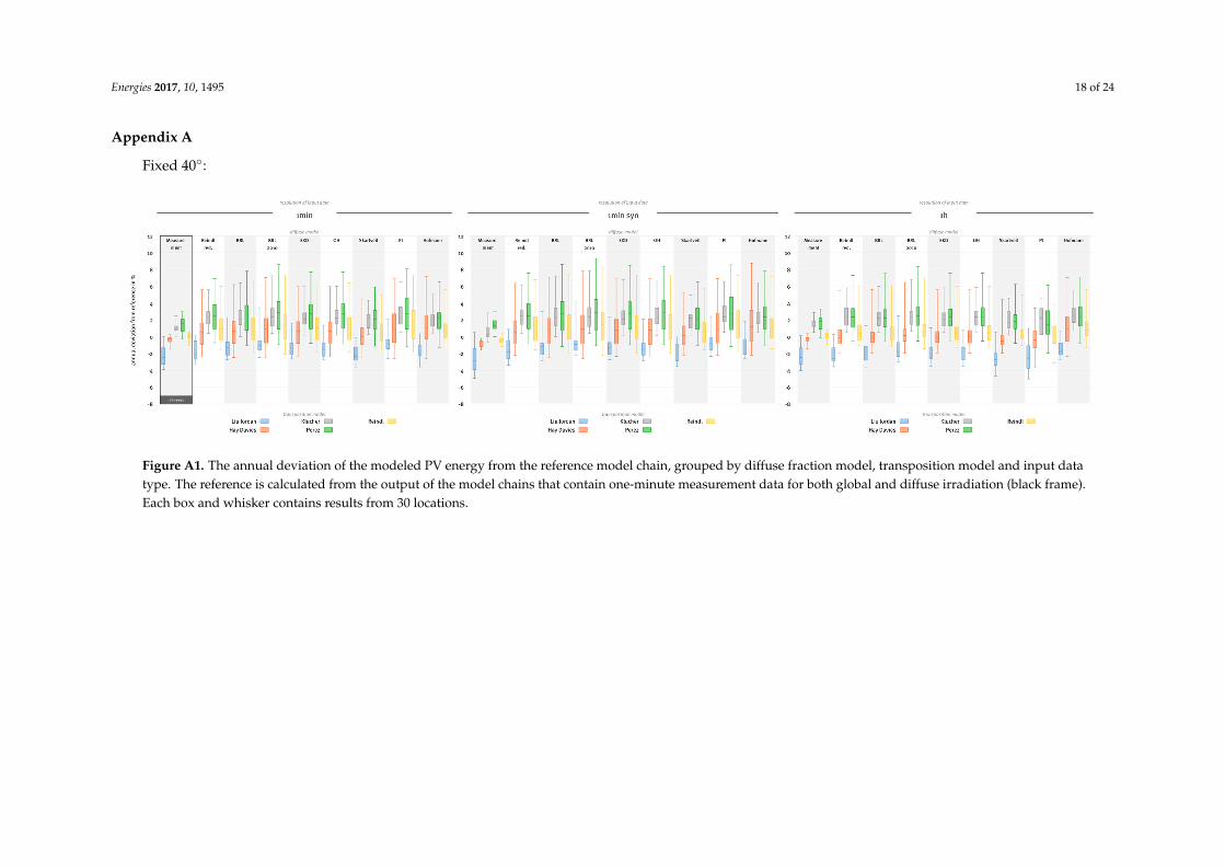
Figure A2. Same plot type as Figure A1, but for modules with optimal tilt. Corresponds to Figure 8.

Two Axis Tracking:

Figure A3. Same plot type as Figure A1, but for modules with two-axis tracking. Note the different y scale in comparison to Figures A1 and A2.

Figure A2. Same plot type as Figure A1, but for modules with optimal tilt. Corresponds to Figure 8.

Two Axis Tracking:

Energies 2017, 10, 1495 18 of 23

Optimum Tilt:

Figure A2. Same plot type as Figure A1, but for modules with optimal tilt. Corresponds to Figure 8.

Two Axis Tracking:

Figure A3. Same plot type as Figure A1, but for modules with two-axis tracking. Note the different y scale in comparison to Figures A1 and A2. Figure A3. Same plot type as Figure A1, but for modules with two-axis tracking. Note the different y scale in comparison to Figures A1 and A2.

Energies 2017, 10, 1495 20 of 24

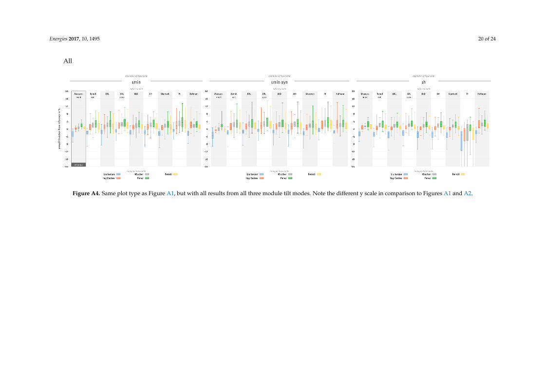
All

Energies 2017, 10, 1495 19 of 23

All

Figure A4. Same plot type as Figure A1, but with all results from all three module tilt modes. Note the different y scale in comparison to Figures A1 and A2. Figure A4. Same plot type as Figure A1, but with all results from all three module tilt modes. Note the different y scale in comparison to Figures A1 and A2.

Energies 2017, 10, 1495 21 of 24Energies 2017, 10, x FOR PEER REVIEW 20 of 23

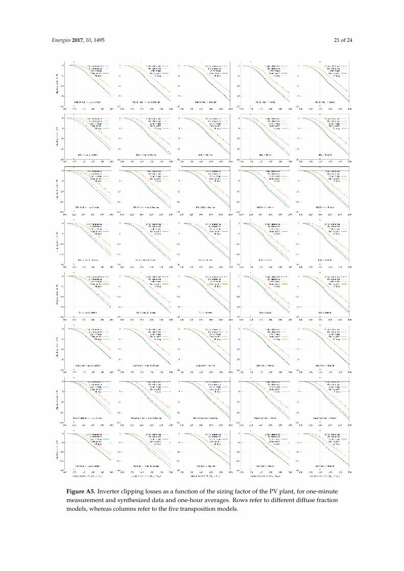
Figure A5. Inverter clipping losses as a function of the sizing factor of the PV plant, for one-minute measurement and synthesized data and one-hour averages. Rows refer to different diffuse fraction models, whereas columns refer to the five transposition models.

Figure A5. Inverter clipping losses as a function of the sizing factor of the PV plant, for one-minutemeasurement and synthesized data and one-hour averages. Rows refer to different diffuse fractionmodels, whereas columns refer to the five transposition models.

Energies 2017, 10, 1495 22 of 24Energies 2017, 10, 1495 21 of 23

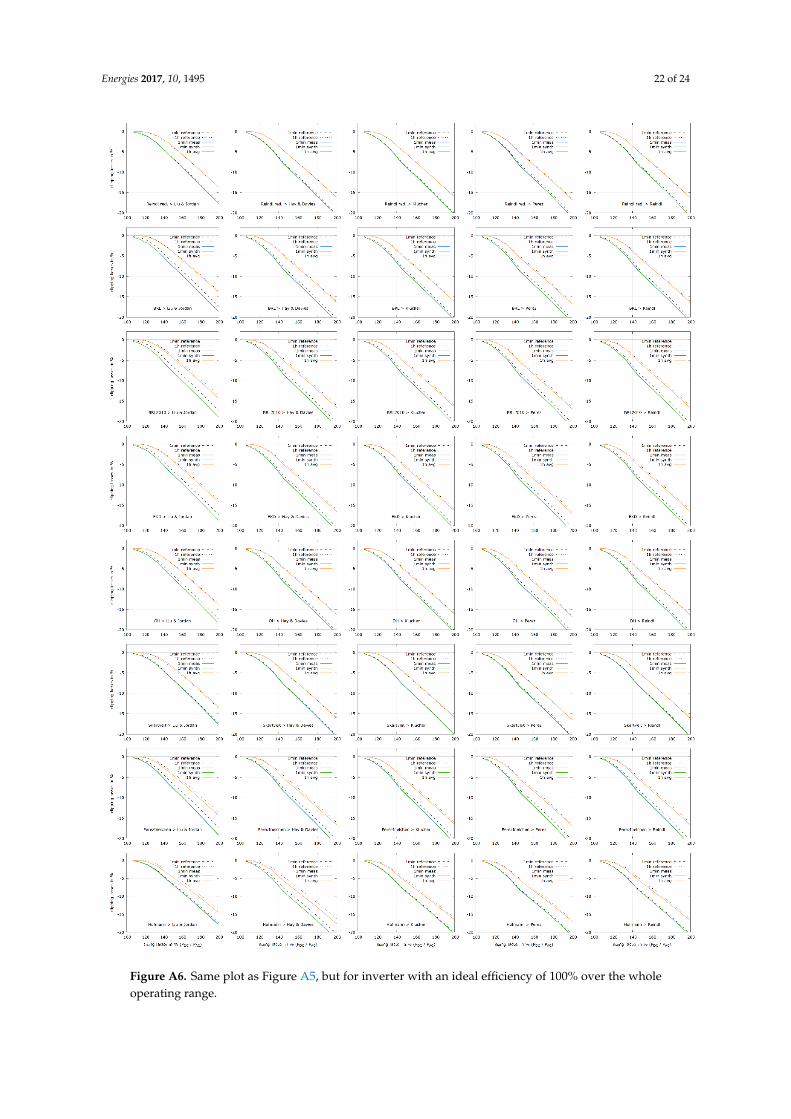
Figure A6. Same plot as Figure A5, but for inverter with an ideal efficiency of 100% over the whole operating range.

Figure A6. Same plot as Figure A5, but for inverter with an ideal efficiency of 100% over the wholeoperating range.

Energies 2017, 10, 1495 23 of 24

References

1. König-Langlo, G.; Sieger, R. Report of the working group BSRN—Baseline Surface Radiation Network.AIP Conf. Proc. 2013, 1531, 668–671.

2. Köppen, W. Klassifikation der Klimate nach Temperatur, Niederschlag und Jahresablauf (Classificationof climates according to temperature, precipitation and seasonal cycle). Petermanns Geogr. Mitt. 1918, 64,193–203.

3. Bourges, B. Improvement in solar declination computation. Sol. Energy 1985, 35, 367–369. [CrossRef]4. Hofmann, M.; Riechelmann, S.; Crisosto, C.; Mubarak, R.; Seckmeyer, G. Improved synthesis of global

irradiance with one-minute resolution for PV system simulations. Int. J. Photoenergy 2014, 2014. [CrossRef]5. Remund, J. Neue Modelle für die Realistische Generierung von Minutenwerten. Available online: https://www.

researchgate.net/publication/315767163_Neue_Modelle_fur_die_realistische_Generierung_von_Minutenwerten(accessed on 25 September 2017).

6. HAY, J.E.; Davies, J.A. Calculation of the Solar Radiation Incident on an Inclined Surface. In Proceedings ofthe First Canadian Solar Radiation Data Workshop, Toronto, ON, Canada, 17–19 April 1978.

7. Hofmann, M.; Hunfeld, R. PV*SOL Simulation Core; Valentin Software: Berlin, Germany, 2017.8. German Institute for Standardisation. Daylight in Interiors; Principles; DIN: Berlin, Germany, 1985.9. Reda, I.; Nrel, A.A. Solar Position Algorithm for Solar Radiation Applications (Revised). Sol. Energy 2004, 76,

577–589. [CrossRef]10. Gueymard, C.A.; Ruiz-Arias, J.A. Extensive worldwide validation and climate sensitivity analysis of direct

irradiance predictions from 1-min global irradiance. Sol. Energy 2016, 128, 1–30. [CrossRef]11. Hofmann, M.; Seckmeyer, G. A New Model for Estimating the Diffuse Fraction of Solar Irradiance for

Photovoltaic System Simulations. Energies 2017, 10, 248. [CrossRef]12. Quaschning, V. Vergleich und Bewertung Verschiedener Verfahren zur Solarstrahlungsbestimmung.

Available online: https://volker-quaschning.de/downloads/Sofo2002_1.pdf (accessed on 25 September 2017).13. Kambezidis, H.D.; Psiloglou, B.E.; Gueymard, C. Measurements and Models for Total Solar Irradiance on

Inclined Surface in Athens, Greece. Sol. Energy 1994, 53, 177–185. [CrossRef]14. Wong, L.T.; Chow, W.K. Solar radiation model. Appl. Energy 2001, 69, 191–224. [CrossRef]15. Dervishi, S.; Mahdavi, A. Computing diffuse fraction of global horizontal solar radiation: A model

comparison. Sol. Energy 2012, 86, 1796–1802. [CrossRef] [PubMed]16. Reindl, D.T.; Beckman, W.A.; Duffie, J.A. Diffuse fraction corrections. Sol. Energy 1990, 45, 1–7. [CrossRef]17. Erbs, D.G.; Klein, S.A.; Duffie, J.A. Estimation of the diffuse radiation fraction for hourly, daily and

monthly-average global radiation. Sol. Energy 1982, 28, 293–302. [CrossRef]18. Orgill, J.F.; Hollands, K.G.T. Correlation equation for hourly diffuse radiation on a horizontal surface.

Sol. Energy 1977, 19, 357–359. [CrossRef]19. Boland, J.; Ridley, B. Models of diffuse solar fraction. In Modeling Solar Radiation at the Earth’s Surface; Springer:

Berlin/Heidelberg, Germany, 2008; pp. 193–219.20. Ridley, B.; Boland, J.; Lauret, P. Modelling of diffuse solar fraction with multiple predictors. Renew. Energy

2010, 35, 478–483. [CrossRef]21. Skartveit, A.; Olseth, J.A. A model for the diffuse fraction of hourly global radiation. Sol. Energy 1987, 38,

271–274. [CrossRef]22. Perez, R.; Ineichen, P.; Seals, R.; Michalsky, J.; Stewart, R. Modeling daylight availability and irradiance

components from direct and global irradiance. Sol. Energy 1990, 44, 271–289. [CrossRef]23. Liu, B.Y.H.; Jordan, R.C. The interrelationship and characteristic distribution of direct, diffuse and total solar

radiation. Sol. Energy 1960, 4, 1–19. [CrossRef]24. Klucher, T.M. Evaluation of models to predict insolation on tilted surfaces. Sol. Energy 1979, 23, 111–114.

[CrossRef]25. Perez, R.; Seals, R.; Ineichen, P.; Stewart, R.; Menicucci, D. A new simplified version of the perez diffuse

irradiance model for tilted surfaces. Sol. Energy 1987, 39, 221–231. [CrossRef]26. Reindl, D.T.; Beckman, W.A.; Duffie, J.A. Evaluation of hourly tilted surface radiation models. Sol. Energy

1990, 45, 9–17. [CrossRef]27. Temps, R.C.; Coulson, K.L. Solar radiation incident upon slopes of different orientations. Sol. Energy 1977,

19, 179–184. [CrossRef]

Energies 2017, 10, 1495 24 of 24

28. Muneer, T. Solar radiation model for Europe. Build. Serv. Eng. Res. Technol. 1990, 11, 153–163. [CrossRef]29. Olmo, F.; Vida, J.; Foyo, I.; Castro-Diez, Y.; Alados-Arboledas, L. Prediction of global irradiance on inclined

surfaces from horizontal global irradiance. Energy 1999, 24, 689–704. [CrossRef]30. Gueymard, C. An anisotropic solar irradiance model for tilted surfaces and its comparison with selected

engineering algorithms. Sol. Energy 1987, 38, 367–386. [CrossRef]31. Badescu, V. 3D isotropic approximation for solar diffuse irradiance on tilted surfaces. Renew. Energy 2002, 26,

221–233. [CrossRef]32. Yang, D. Solar radiation on inclined surfaces: Corrections and benchmarks. Sol. Energy 2016, 136, 288–302.

[CrossRef]33. Ineichen, P. Global Irradiance on Tilted and Oriented Planes: Model Validations; Technical Report;

University Geneva: Geneva, Switzerland, October 2011.34. Loutzenhiser, P.G.; Manz, H.; Felsmann, C.; Strachan, P.A.; Frank, T.; Maxwell, G.M. Empirical validation of

models to compute solar irradiance on inclined surfaces for building energy simulation. Sol. Energy 2007, 81,254–267. [CrossRef]

35. Gueymard, C.A. From Global Horizontal to Global Tilted Irradiance: How Accurate Are Solar EnergyEngineering Predictions in Practice? Available online: http://www.solarconsultingservices.com/Gueymard-Tilted%20radiation%20models%20performance-ASES08.pdf (accessed on 25 September 2017).

36. Demain, C.; Journée, M.; Bertrand, C. Evaluation of different models to estimate the global solar radiation oninclined surfaces. Renew. Energy 2013, 50, 710–721. [CrossRef]

37. Gulin, M.; Vašak, M.; Baotic, M. Estimation of the Global Solar Irradiance on tilted Surfaces. Available online:http://www.apr.fer.hr/old/papers/EDPE2013_solar.pdf (accessed on 25 September 2017).

38. Souka, A.F.; Safwat, H.H. Determination of the optimum orientations for the double-exposure, flat-platecollector and its reflectors. Sol. Energy 1966, 10, 170–174. [CrossRef]

39. Laboratories, S.N. ASHRAE Model—PV Performance Modeling Colaborative. Available online: http://pvpmc.org/modeling-steps/shading-soiling-and-reflection-losses/incident-angle-reflection-losses/ashre-model/(accessed on 25 September 2017).

40. Meteonorm: Irradiation Data for Every Place on Earth. Available online: http://www.meteonorm.com/images/uploads/downloads/broschuere-mn-7.1.pdf (accessed on 25 September 2017).

41. Yadav, A.K.; Chandel, S.S. Tilt angle optimization to maximize incident solar radiation: A review. Renew. Sustain.Energy Rev. 2013, 23, 503–513. [CrossRef]

42. Hafez, A.Z.; Soliman, A.; El-Metwally, K.A.; Ismail, I.M. Tilt and azimuth angles in solar energyapplications—A review. Renew. Sustain. Energy Rev. 2017, 77, 147–168. [CrossRef]

43. Beringer, S.; Schilke, H.; Lohse, I.; Seckmeyer, G. Case study showing that the tilt angle of photovoltaic plantsis nearly irrelevant. Sol. Energy 2011, 85, 470–476. [CrossRef]

44. 2017 German Renewable Energy Law (EEG 2017). Available online: https://www.gesetze-im-internet.de/eeg_2014/BJNR106610014.html (accessed on 10 August 2017).

45. Burger, B.; Rüther, R. Inverter sizing of grid-connected photovoltaic systems in the light of local solar resourcedistribution characteristics and temperature. Sol. Energy 2006, 80, 32–45. [CrossRef]

46. Ransome, S.; Funtan, P. Why Hourly Averaged Measurement Data Is Insufficient to Model PV PerformanceAccurately. Available online: http://www.steveransome.com/PUBS/2005Barcelona_6DV_4_32.pdf (accessed on25 September 2017).

© 2017 by the authors. Licensee MDPI, Basel, Switzerland. This article is an open accessarticle distributed under the terms and conditions of the Creative Commons Attribution(CC BY) license (http://creativecommons.org/licenses/by/4.0/).