DI

SC

US

SI

ON

P

AP

ER

S

ER

IE

S

Forschungsinstitut zur Zukunft der ArbeitInstitute for the Study of Labor

Inequality in Vietnamese Urban-Rural Living Standards, 1993-2006

IZA DP No. 4987

June 2010

Huong Thu LeAlison L. Booth

Inequality in Vietnamese Urban-Rural

Living Standards, 1993-2006

Huong Thu Le Australian National University

Alison L. Booth

University of Essex, Australian National University and IZA

Discussion Paper No. 4987 June 2010

IZA

P.O. Box 7240 53072 Bonn

Germany

Phone: +49-228-3894-0 Fax: +49-228-3894-180

E-mail: iza@iza.org

Any opinions expressed here are those of the author(s) and not those of IZA. Research published in this series may include views on policy, but the institute itself takes no institutional policy positions. The Institute for the Study of Labor (IZA) in Bonn is a local and virtual international research center and a place of communication between science, politics and business. IZA is an independent nonprofit organization supported by Deutsche Post Foundation. The center is associated with the University of Bonn and offers a stimulating research environment through its international network, workshops and conferences, data service, project support, research visits and doctoral program. IZA engages in (i) original and internationally competitive research in all fields of labor economics, (ii) development of policy concepts, and (iii) dissemination of research results and concepts to the interested public. IZA Discussion Papers often represent preliminary work and are circulated to encourage discussion. Citation of such a paper should account for its provisional character. A revised version may be available directly from the author.

IZA Discussion Paper No. 4987 June 2010

ABSTRACT

Inequality in Vietnamese Urban-Rural Living Standards, 1993-2006*

Using data from five waves of the Vietnam Household Living Standard Survey, we find evidence of significant urban-rural expenditure inequality. Urban-rural inequality in Vietnam increased dramatically from 1993 to 1998, and peaked in 2002 before reducing slightly in 2004, and significantly in 2006. The urban-rural gap also monotonically increases across the expenditure distribution. We use a variant of the Oaxaca-Blinder decomposition method, applied to the unconditional quantile regression method of Firpo, Fortin and Lemieux (2009), to explain the components of the per capita expenditure differentials between urban and rural households at selected quantiles of the distribution. We also compare these estimates with those at mean obtained by OLS. Our results show a number of factors contributing significantly to the high urban-rural gap. These include inter-group differences in education, household demographic structure, industrial structure and their related returns. Adjusting the average characteristics of rural households to those of urban households will reduce about a half of the overall urban-rural expenditure gap. A significant part of the remaining unexplained component lies in the intercept differences; that is, the inter-group differences in other factors not captured in the model that favor urban households. JEL Classification: O18, O53, C13 Keywords: urban-rural inequality, Vietnam, unconditional quantile regression,

Oaxaca decomposition Corresponding author: Alison L. Booth Department of Economics University of Essex Wivenhoe Park, CO4 3SQ United Kingdom E-mail: albooth@essex.ac.uk

* We are grateful to Bob Breunig, Nicole Fortin, Tue Gorgens, Ben Jann and Thomas Lemieux for their advice on the estimation method. For other helpful suggestions, we thank Paul Glewwe, Andrew Leigh, Amy Liu, Brian McCaig, Ha Trong Nguyen, Mathias Sinning, as well as seminar and conference participants at the Research School of Economics and the Second Economic Workshop on Vietnam at the Australian National University, the 2010 Pacific Conference for Development Economics at the University of Southern California, the 7th Midwest International Economic Development Conference at the University of Minnesota. Part of this research was funded by the Australian Research Council. Any errors are our own.

1

1. Introduction

Vietnam has experienced continuously high economic growth since the transition from a

centrally planned and controlled economy to a market economy began in 1986. The average

annual growth rate of Gross Domestic Product of Vietnam from 1989 to 2008 is 7.4% (ADB,

2008). Over the period, Vietnam has had one of the fastest improvements in living standards

and the greatest reduction in poverty in the world. With an annual per capita income over

US$1000 in 2008, Vietnam is predicted to become a middle income country by 2010 (World

Bank, 2008).

However, this period of transition and opening up of the economy has seen a widening

of the gap between the rich and the poor, and between urban and rural areas. Closing the urban-

rural gap is now one of the top priorities in the Vietnamese government’s development strategy.

It is at the center of public debates and in the press, and is a major concern of ordinary

Vietnamese people and international donors.1 Establishing what factors contribute to this urban-

rural gap is one of the primary goals of this paper.

Two earlier studies used data from the first two Vietnam Living Standard Surveys

(VLSSs), undertaken in 1992/1993 and 1997/1998, to examine this issue. These papers, by

Nguyen, Albrecht, Vroman and Westbrook (2007) and Le and Fesselmeyer (2008), found a

significant increase in urban-rural expenditure inequality over the period 1993 to 1998, and

showed that urban-rural expenditure inequality plays the most important role in explaining

national inequality. We extend their analysis, using new methods, up to 2006.

First, we use inequality indices and descriptive statistics to establish an overall picture of

urban-rural inequality in Vietnam from 1993 to 2006, and compare urban-rural inequality with

inequality across other characteristics over the period. We also briefly compare urban-rural

1 For example, see To (2008), Rama (2008), Tran (2008), Ngoc (2008).

2

inequality in Vietnam with other countries at the same level of development and with those at a

similar stage of transition. Next, we use the unconditional quantile regression method of Firpo,

Fortin and Lemieux (2009) to estimate the determinants of per capita household expenditure in

urban and rural households. This is done separately for each of five waves of data from 1993 to

2006. Finally, we use a variant of the Oaxaca-Blinder decomposition method, applied to the

unconditional quantile regression method, to explain the components of the real per capita

household expenditure differentials between urban and rural households at selected quantiles of

the distribution, and to explore how these factors changed over time. We also explore the

factors contributing to the increase in expenditure of urban and rural households.

The remainder of the paper is set out as follows. Section 2 summarizes Vietnam’s

transition and urban development, and reviews existing studies on urban-rural inequality in

Vietnam. Section 3 describes the data, while Section 4 provides a profile of urban-rural

inequality from both descriptive statistics and inequality indices analyses. Variables used in our

analysis are described in Section 5, followed in Section 6 by exposition of the Firpo, Fortin and

Lemieux (2009) method of unconditional quantile regression, and our application to it of the

Oaxaca decomposition in section 7. The conclusions and policy implications are given in the

final section.

2. Background

2.1. Vietnam’s transition and urban development

The population of Vietnam, situated in Southeastern Asia and bordering the Pacific, stood at 86

million in 2008. With only 28% of the total population living in urban areas (GSO Vietnam,

2009), the urban population rate of Vietnam is low compared to other countries in the East Asia

region and the world, and reflects the lack of urban development in the country.2 As with many

countries in the region, Vietnam was an agricultural economy prior to 1945, with over 90% of

2 The percentage of East Asian population that is urban is 45%, as compared with 48% for the entire world (UNDP, 2008).

3

the population living in rural areas, where rice was the major crop of cultivation. From 1945 to

1975, Vietnam experienced 30 years of war.3 After the war ended, Vietnam was a centrally

command and control economy. During this period, the urban population was kept stable at

around 19%. By the end of the centrally planned period, Vietnam was one of the poorest

countries in the world.

The transition from a centrally planned economy to a market-oriented economy in

Vietnam started in 1986. Since then, Vietnam has experienced continuously high economic

growth and a significant change in industrial structure. Between 1990 and 2008, the industry

and services share of GDP rose from 68% to 83%, while the agricultural share declined from

32% to 17% (GSO Vietnam, 2009). 4 Along with this significant change in the structure of the

economy, Vietnam is experiencing a high rate of urbanization, with the proportion of

population living in urban areas increasing from 19% in 1986 to 28% in 2008 (UNDP, 2008).

However, there is unbalanced growth between urban and rural areas. The urban areas of

Vietnam are benefiting from their initial advantages of geographical, infrastructure

characteristics and industrial clustering and thus becoming growth centers attracting foreign

investment. In contrast, rural areas are viewed as relatively inefficient and by-passed by

development.5 According to the World Bank (2004), while the urban areas of Vietnam contain

only 25% of the population, they account for up to 70% of national economic growth.6 This

unbalanced growth creates a marked unevenness between urban and rural areas in terms of

employment opportunities and living standard improvements. Therefore, even though the

3 For more details of urban development in Vietnam during the war period from 1945 to 1975, see Boothroyd et al. (2000). 4 See Appendix [1] for more details. 5 For example, see Mundle et al. (1997), Glewwe et al. (2002), Phan (2002), World Bank (2004). 6 According to an estimation of Mekong Economics (2002) from the data of Ministry of Investment and Planning, during the period from 1988 to 2001, foreign direct investment (FDI) in Vietnam focused in certain key industrial areas such as Ho Chi Minh City, Dong Nai, Ba Ria Vung Tau, Binh Duong in the South, and Ha Noi, Hai Duong, Hai Phong, Quang Ninh in the North. These key areas in the North and the South accounted for around 80% of licensed projects and registered capital. The amount of (FDI) to the two biggest cities, Ha Noi and Ho Chi Minh City, alone accounted for 49% of the total FDI in Vietnam. According to General Statistics Office of Vietnam (2008) during the period from 2000 to 2007, FDI continued concentrate in some advantage business regions in the Southeast and Red River Delta. The numbers as well as amount of FDI capital in other regions were few.

4

overall standard of living improved remarkably over the last two decades, poverty remains

widespread and overwhelmingly found in rural areas. For example, in 2004, 25% of rural

people lived in poverty as compared with an urban poverty rate of 3.6% (VASS, 2007). Recent

studies about overall inequality in Vietnam - by the Asian Development Bank (2007) using per

capita expenditure and McCaig (2009) using per capita income - emphasize that this urban-rural

inequality has been the most important contributing factor to overall inequality in Vietnam

between 1993 and 2006.

2.2. Literature review and the contributions of our study

The changes since the transition in 1986, from a centrally planned closed economy to a market-

oriented open economy, make Vietnam an interesting country in which to study inequality.

While a number of studies examine inequality in Vietnam, they focus on issues such as poverty

and inequality, ethnic inequality, and rural inequality and urban inequality examined separately.

Little attention has been given specifically to urban-rural inequality, the focus of the present

paper. As noted above, there are to our knowledge only two studies examining urban-rural

inequality in Vietnam: Nguyen, Albrecht, Vroman and Westbrook (2007) and Le and

Fesselmeyer (2008). Both use data from the first two waves of the VLSS undertaken in 1993

and 1998, but they adopt different estimation techniques to that utilized in this paper.

Nguyen, Albrecht, Vroman and Westbrook (2007) apply the quantile regression based

decomposition proposed by Machado and Mata (2005), while Le and Fesselmeyer (2008) apply

the Dinardo et al. (1996) semi-parametric decomposition method.7 They find that the significant

7 The Dinardo et al. (1996) decomposition and the Machado and Mata (2005) quantile regression based decomposition both rely on the construction of the counterfactual distribution. The Dinardo et al. (1996) method involves first estimating a probit model to find the probability of a household with a given characteristics living in an urban area. The predicted probability is then used to calculate the reweighting factor. Next, the re-weighting factor is used as a new weight to find the counterfactual density of the rural per capita household expenditure, which is the per capita expenditure that rural households would have if they were endowed with the same characteristics as urban households, but received the rural return. The Machado and Mata (2005)‘s quantile regression based decomposition involves first estimating the determinants of per capita household expenditure using a quantile regression for the rural sample. Then the counterfactual distribution for urban sample is constructed from the actual urban characteristics and the estimated rural returns. By replacing the estimated coefficients for each variable, this method can capture the contribution from each factor. However, in both methods, Dinardo et al (1996) and Machado and Mata (2005), the order of decomposition (or, in other words the choice of the counterfactual) is important. Additionally, the method of quantile

5

increase in the urban-rural gap from 1993 to 1998 is the most important factor explaining the

increase in overall expenditure inequality. Nguyen, Albrecht, Vroman and Westbrook (2007)

find that, in 1993 across all points in the expenditure distribution, most of the urban-rural gap

comes from the characteristic gap. As the Vietnamese economy became more marketized in

1998, the returns gap was found to play a more important role in the composition of the overall

urban-rural gap. In addition, the differences in household structure, human capital and ethnicity

are found to be the major contributing factors to the urban-rural gap in 1993 and 1998. The

increase in returns to education plays the most important role in the widening the gap during the

period. The study of Le and Fesselmeyer (2008), using a different decomposition method

comes to the same conclusions as that of Nguyen, Albrecht, Vroman and Westbrook (2007).

Although the methods applied by Nguyen, Albrecht, Vroman and Westbrook (2007) and

Le and Fesselmeyer (2008) allow the authors to investigate the urban-rural inequality at

different points along the distribution, in both methods, the results of decomposition are

sensitive to the choice of the counterfactuals (Firpo et al. 2007). Indeed, Le and Fesselmeyer

(2008) demonstrate that the use of different counterfactuals will give different results.

What are the contributions of our study to the literature on urban-rural inequality in

Vietnam? They are threefold, with the first two being methodological while the last relates to

the extended data window we use.

Our first contribution is to use the new method of unconditional quantile regression of

Firpo, Fortin and Lemieux (2009) to examine the determinants of urban and rural per capita

expenditure at selected percentiles along the distribution. We compare this with OLS at the

mean. The advantage of the unconditional quantile regression over the traditional conditional

quantile regression of Koenker and Bassett (1978) is that its estimated coefficients are

regression based decomposition proposed by Machado and Mata (2005) involves many simulations and thus requires computationally intensive.

6

explained as the impact of changes in the distribution of explanatory variables on the quantiles

of the unconditional distribution of the dependent variable. Therefore, we can apply the Oaxaca

decomposition method directly to the estimation results from the unconditional quantile

regression without having to do many simulations as in the method of quantile regression

decomposition proposed by Machado and Mata (2005). This represents our second contribution

to the literature, since we are the first to apply a variation of the Oaxaca-Blinder decomposition

method to the unconditional quantile regression. This allows us to separate the contribution of

returns and characteristics from each explanatory variable. In addition, we apply the method of

Yun (2005) to transform the estimated coefficients, making our decomposition results

consistent with the choice of omitted groups in the presence of categorical variables. By doing

so, the decomposition results with the new transformed coefficients are equivalent to the

average estimates of returns and characteristics gap with varying reference groups.

Our third contribution is to examine a longer period than previous studies, which have

used the first two waves of the VLSS (1993 and 1998). We extend the period to use five waves

of the Vietnam Living Standard Surveys covering the period 1993 to 2006. 8 As noted above,

this period is important for Vietnam not only because of its continuously high economic

growth, but also because of significant changes in the structure of the economy and its

accelerated integration into the world market. These have led to a marked change in distribution

outcome.

3. Data and Sample

The first two waves of data that we use are from the Vietnam Living Standard Surveys (VLSSs)

undertaken in 1992/1993 and 1997/1998, while the next three waves are from the Vietnam

Household Living Standard Surveys (VHLSS) undertaken in 2002, 2004 and 2006. These are

8 Vietnam resumed relations with the International Monetary Fund and the World Bank in 1992; established political normalization with the United States (US) in 1994; became a member of the Association of Southeast Asian Nations (ASEAN) in 1995, ASEAN Free Trade Area in 1996, Asia-Pacific Economic Cooperation in 1998; signed the Bilateral Trade Agreement with the US in 2000; and joined World Trade Organization in 2006.

7

nationally representative surveys conducted by Vietnam’s General Statistics Office with

technical assistance from the World Bank and UNDP. Although the subsequent VHLSS

questionnaires were simplified compared to the first two waves of VLSS, the question design in

both follows the standard set for the Living Standard Measurement Surveys of the World

Bank.9 As a result, these surveys contain comprehensive and comparable information across

years, thus facilitating welfare analysis at a household level. The sample consists of 4800, 6000,

29530, 9188, and 9189 households in VLSS1993, VLSS 1998, VHLSS 2002, VHLSS 2004 and

VHLSS 2006, respectively. In each wave, there are two sets of questionnaires: a household

questionnaire and a community questionnaire. The household questionnaire contains rich

information on the demography, education, health, employment, expenditures, credit, saving

and poverty reduction participation at the household and individual level. The community

questionnaire collects information on the demographic, health, education and infrastructure of

all rural communities.

There are 4,000 households surveyed in VLSS 1993 who were re-interviewed in 1998.

While there are also panel samples from the last 3 waves - VHLSS 2002, 2004 and 2006 - there

are no households re-interviewed between the VLSS and the VHLSS. For our purpose of

observing the whole period and making our observed sample nationally representative, we

analyze all five waves in separate cross-sections.

The last column of Table [1] indicates the sample size separately, by urban and rural

categories.10 Thus, for example, the 1993 VLSS comprises 1,072 urban and 3,727 rural

9 For more details about the sample designs, such as the units of clustering, stratifications, and weight constructions in each waves, see World Bank (1998), World Bank (2001) and General Statistics Office of Vietnam (2006). 10 The survey samples only cover the registered residence. In VLSS 1993, the total number of surveyed households is 4800, but one household (coded 10301) with data on expenditure exists only for two months and is excluded from the sample, leaving the total number of observations in 1993 at 4799. In VLSS 1998, the total number of households being surveyed in the expenditure sample is 6002, but three households are excluded because two household (coded 1302 and 11916) lack information on some sections and another household (coded 7506) contains only one elderly person who lives alone and has meals with their children’s family so there is a lack of information on food expenditure. Thus, there are 5999 observations left in VLSS 1998 - see World Bank (1998 a. b) World Bank (2001) and GSO Vietnam (2006) for more details.

8

households. Column [2] reports the percentage of urban households in the sample, adjusted by

household weights. These numbers approximate the actual percentage of urban people.

[Table 1 about here]

To compare the difference between urban and rural living standards, we use total real per

capita yearly expenditure (RPCEXP).11 This is calculated by dividing total household

expenditure by the household size. 12 Although income is usually the best indicator for

measuring inequality, expenditure is preferred for developing countries. The reasons are

discussed in depth in Deaton (1997), Van de Walle et al. (2001) and Glewwe et al. (2002).13 We

calculate real per capita expenditure by using the current per capita expenditure adjusted for the

monthly and the regional price indices then converting to the current price of Jan 2006 for

comparative purposes.14

11 The calculation of expenditure follows the formula used in the World Bank Living Standard Measurement Survey. Household total expenditure is the sum of expenditure on food and non-food items. Specifically, food expenditure includes both expenditure on purchased items and home-produced products. The value of consumption from home-produced products is calculated using the total quantity of consumed multiplied by the value of such consumption if it was purchased in the market. Non-food expenditure includes expenditures on daily items, utilities, transportation, entertainment, education, health, the imputed values of household appliances or other consumer durables to be consumed in the year, house rent or, for those who live in their own house, the imputed depreciation value of the house in the year for those who live in their own house. Expenditures on consumer durables, house building, social funds, and the purchase of gold, silver, precious germs, stocks or bonds are excluded. Thus the expenditure calculated from the survey is a relatively good measure of living standard - see World Bank (1998b), Glewwe (2003) and Glewwe (2005) for more details. 12 Households differ in size and in the age of the household members. Theories suggest that larger are likely to be benefit from the economies of scale in household expenditure (i.e., larger households can enjoy the same living standard, with lower per capita expenditure, as smaller households). In addition, adults and children are likely to have different needs and consume a different proportion of the total household expenditure, (see Deaton (1997) for more details about the problem of equivalent scale in calculating household per capita expenditure). By dividing total household expenditure by the number of people in the household, and then using total household per capita expenditure as the measure of welfare for each member of the household, we assume that everyone in the household is identical and has the same needs. 13 Reasons for preferring expenditure over income are: first, income tends to be under-reported in developing countries, whereas questions on expenditure are answered more honestly. Second, a large proportion of people in developing countries are engaged in self-employment - including farm work. Income from self-employment and agriculture activities is seasonal and thus fluctuates. In addition, estimation of income from agricultural activities often suffers from measurement error. For a given period of time, income only raises the living standard if it is consumed. Therefore expenditure is smoother than income for a longer period, and is thus a better indicator of welfare and living standard for a developing country such as Vietnam. 14 The price deflator is computed from the monthly price indexes released by the GSO of Vietnam. See Appendix [2] for more details.

9

4. Overall picture of urban-rural inequality in Vietnam, 1993-2006

4. 1. Urban-rural inequality from inequality indices analysis

This section uses the Gini and Theil indices to provide a comprehensive picture of urban-rural

expenditure inequality in Vietnam during 1993 to 2006 period. Table [2] reports inequality

indices across years for the whole nation as well as by urban-rural sectors. Using the Gini

index, it can be seen that national inequality increased from 1993 to 2002 (the Gini coefficient

increased from 0.34 in 1993 to 0.37 in 2002), remained unchanged from 2002 to 2004 and

decreased from 2004 to 2006 (the Gini coefficient reduced from 0.37 in 2004 to 0.36 in 2006).

How does this compare with other countries with a comparable level of GDP per capita?

Table [3] demonstrates that inequality in Vietnam in 2004 is 0.37, which is lower than

Cambodia (whose Gini was 0.42 in 2004), is equal to that of India, and is a little bit higher than

in Indonesia (whose Gini was 0.34 in 2002). What about other countries at a comparable

transition pattern? While Vietnam has the same pattern of economic transition as China, and is

similar to some extent to Russia and Poland, the Gini index of Vietnam in 2004 is lower. For

example, China had a Gini of 0.47 in 2004; Russia a Gini of 0.40 in 2002; and Poland a Gini of

0.35 in 2002. However, we cannot draw any precise conclusions about the comparative

inequality levels between Vietnam and these last countries because each has different level of

development as measured by per capita GDP. More positively, the trend of inequality in

Vietnam from 2002 to 2006 indicates that it remained stable then reduced slightly during the

recent period of high economic growth.

[Table 2 and 3 about here]

Inequality is higher in urban than rural households in all waves. Furthermore, the

evolution of inequality indices is different in the urban and rural sectors. In the urban sector,

inequality increased from 1993 to 2002 then decreased from 2002 to 2006, with the Gini

increasing from 0.34 in 1993 to 0.35 in 2002 then decreasing to 0.33 in 2004 and remaining

10

stable in 2006. In contrast, in the rural sector, inequality decreased slightly from 1993 to 1998

then increased from 1998 to 2006, with the Gini dropping from 0.28 in 1993 to 0.27 in 1998,

and then increasing steadily to the value of 0.30 in 2006.

While the results based on the inequality indices provide a picture of overall inequality,

they do not enlighten us as to the composition of overall inequality nor indicate the contribution

of between- and within-group differences that are the focus of our interest. Tables 4.a to 4.c

address these issues by using the Theil decomposition to look at the components of between-

and within-group inequality across different characteristics of the households. These show the

following. First, urban-rural between-group inequality makes the largest contribution to overall

inequality. Specifically, the between-group urban-rural inequality accounted for 21% of the

overall inequality in 1993, and this increased rapidly to 31% in 1998, 33% in 2002 and then fell

slightly to 31% in 2004 and decreased to 25% in 2006 (Table 4a and Figure1). Second, consider

ethnicity. Inequality between the majority ethnic group (Kinh) and the minority ones increased

continuously over time from 2% in 1993 to 8% in 2006 (Table 4a). Third, consider education.

Between-groups inequality by household head’s education increased remarkably over time,

from 8% in 1993 to 21% in 2006 (Table 4b). Fourth, turning to the household head’s

employment status, within-group inequality is increasing in households where the head is

working in the private sector, working in the service sector and households where the head is

elderly (Table 4c). Fifth, inequality between groups by other household head characteristics

(such as gender, marital status and age group), is small and rather stable between 1993 and

2006. Finally, it is interesting to observe an opposite trend in inequality within groups of male-

and female-headed households. While inequality within households headed by males increased

steadily from 1993 to 2006, inequality within households headed by females decreased over the

same period.

[Table 4.a, 4.b, 4.c about here]

11

[Figure 1 about here]

Compared with some other countries in the Asian region, such as India, Indonesia and the

Philippines, Vietnam has higher urban-rural inequality. Vietnam has been outperforming China

in terms of having little increase in urban-rural inequality during the economic transition

process.15

The large differences between urban and rural sectors in levels of per capita expenditure

are why (i) overall inequality is higher than inequality in urban or rural sectors alone, and (ii)

between-group inequality by urban-rural sectors makes the largest contribution to the national

inequality.

4.2. Urban-rural inequality from descriptive statistics and

distributional analysis

Table [1] presented expenditure figures at mean and selected percentiles by urban and rural

households, and showed that per capita expenditure is higher in urban than rural areas. This

pattern holds regardless of the time and the method used to measure expenditure. The urban-

rural expenditure ratio at the mean increased from 1.91 in 1993 to 2.36 in 2002, before

declining to 2.24 in 2004 and 2.01 in 2006.

Table [1] also shows that the real per capita expenditure of the top decile of urban

households is four to five times higher than the real per capita expenditure of the bottom decile.

It is seven to nine times higher than the real per capita expenditure of the bottom decile of rural

households. One of the most striking findings from Table [1], as illustrated in Figure [2], is that

in 1993 the value of the top decile of rural expenditure is almost equal to the median urban

expenditure. The value of the top decile of rural expenditure is under the median urban

expenditure for the years 1998, 2002 and 2004. These figures confirm a long lasting

15 Between urban-rural expenditure inequality in China contributed for 27% to the national inequality in 1985, 40% in 1995, and 44% in 2006. See ADB (2007) for more details.

12

Vietnamese saying, “Giau nha que khong bang keo le thanh thi”, meaning the rural rich are not

as wealthy as the urban poor who work in the city street.

[Figure 2 about here]

Additionally, Figure [3] illustrates the evolution of the urban-rural natural log RPCEXP

gap across the distribution. An important deduction from Figure [3] is that the urban-rural gap,

in terms of log per capita expenditure, is monotonically increasing from the poorer to the richer

groups of the expenditure distribution. From 1993 to 1998, the gap increased at all points in the

distribution. From 1998 to 2002, the gap continued to increase in the middle of the distribution

but decreased slightly in the two tails. While most of the decrease in the urban-rural log per

capita expenditure gap at mean from 2002 to 2004 came from the decrease of the urban-rural

gap in the upper half of the expenditure distribution, all of the decrease at mean from 2004 to

2006 came from the decrease of the urban-rural log per capita expenditure gap at all points in

the distribution.

[Figure 3 about here]

Figure [4] illustrates the distribution of the urban and rural real per capita expenditure

from 1993 to 2006. It can be seen that the urban distribution is more dispersed while the rural

distribution is more concentrated, confirming that there is higher inequality within urban than

rural households. In addition, across all points in the distribution, the urban density lies to the

right of the rural one, showing that urban expenditure is consistently higher than the rural

counterpart at all points along the distribution.

[Figure 4 about here]

There are several possible reasons for the lower per capita expenditure of rural than urban

households. Among them are inter-group differences in education, demographic structure, labor

market activity, and geographic location and the like. For example, as shown in Table [5], the

13

heads of urban households have more years of schooling than those of rural households and

living standards are positively associated with the years of schooling of the household heads.

The urban-rural gap in terms of average years of schooling of the household head increases

over time from 2.08 in 1993 to nearly 2.50 in 2006. Furthermore, urban households have more

favorable demographic characteristics. These include smaller household size, a lower

proportion of children and more laborers. Remarkably, there has been a sharp decrease in the

proportion of children from 28% in 1993 to 18% in 2006 in urban households, and from 36% in

1993 to 23% in 2006 in rural ones. In contrast, there has been a rapid increase in the proportion

of laborers rising from 60% in 1993 to 67% in 2006 in urban households, and from 52% in

1993 to 62% in 2006 in rural households.16 Moreover, urban households are more engaged in

services and in manufacturing sectors where the returns are higher, while rural households are

more engaged in agricultural sector where the returns are relatively low. Furthermore, urban

households received more remittances. Moreover urban households are located in areas with

more favorable geographic and infrastructure conditions.

To what extent are per capita expenditures determined by these characteristics in urban

and rural regions? How much of the inter-group expenditure differential is due to the

differences in average characteristics, returns and other factors not captured in the model? Have

the contributions of these factors changed over time from 1993 to 2006? The results of the

regressions and decompositions in the next section will answer these questions.

16 Vietnam had a population boom after the end of the war in 1975. According to Haub et al. (2009), the population increased rapidly (by 22.7%), to around 24 million people between 1979 and 1989. During the 1990s, Vietnam had a sharp decline in the population growth rate. According to General Statistics Office of Vietnam (2009), the annual population growth of Vietnam in the early 1990s is 2%, in 2000 is 1.4% and in 2006 is 1.2%. The population growth rate of Vietnam in 2006 is higher than that of Korea 0.3%, China 0.5%, and Thailand 0.8%; but is lower than that of The Philippines 1.8%, Malaysia 2.0%, and Indonesia 1.3%.

14

5. Variable descriptions

5.1. The dependent variable

Our dependent variable is real per capita yearly total expenditure.17 We take the natural log of

(RPCEXP), to reduce heteroskedasticity. Hence the estimated coefficients give the percentage

change in expenditure in response to a unit change in the explanatory variable.

5.2. The explanatory variables

The paper exploits the rich and comparable information across five waves to construct a set of

explanatory variables reflecting the demographic, education, employment and other attributes

of the household. Table [5] defines variables and provides summary statistics.

[Table 5 about here]

The first set of explanatory variables are the characteristics of the household head namely

sex, ethnicity, marital status, general experience and general experience squared. 18 Following

Nguyen, Albrecht, Vroman and Westbrook (2007), we use average years of schooling of the

more educated household head or spouse as a measure of the household education. This is

because the most educated household head or spouse is likely to have the bigger impact on

household decisions and thus the household welfare.19 We include dummy variables for

employment status, sectors and industries of employment of the household head. Other

demographic variables include household size and the household proportions of children,

laborers, and the elderly.20

17 See footnotes 11, 12 & 13 for more details. 18 General experience is calculated as age minus years of schooling minus six. Six is the age when children start school in Vietnam. 19 We acknowledge that there may be endogeneity problems in the estimated model. For example, there may be a correlation between of years of schooling of the household head and the error term which includes the variation in other variables not being captured in the model. However, we do not have available any appropriate instruments to solve this problem. 20 In Vietnam, at the age of 15 children finish lower secondary school, and then many of them work, especially in rural areas. Article 6 of the Vietnamese Labour Code (1994) regulates that employees are persons at least 15 years old who are able to work and have entered in to a labour contract. So we identify labourers are those who are over 15 to retirement age, currently not at

15

We estimate the impact of per capita remittances from foreign and domestic sources on

household expenditure separately. Finally, we include six dummies to control for seven regional

differences -this is more detailed than the two regions (North –South) as studied in Nguyen,

Albrecht, Vroman and Westbrook (2007). The reason for doing this comes from our results of

the Theil decomposition by North-South and by seven regions. The between North-South

difference contributes a modest percentage to the overall inequality around 3% to 8% across the

years 1993-2006, compared to the between seven regions difference, which is around 13% to

18% across the years 1993-2006, as will be shown later. So our results will be more accurate at

regional levels. Moreover, the inclusion of the six regional dummies allows us to capture a part

of the geographic differences in prices. According to McCaig (2009) the given regional price

indices of the survey may not fully capture the regional price differences for the case of the

urban South East region in the VLHSS for 2002 and 2004.

6. Estimation methods, model specifications and estimation results

6.1. Estimation methods

Our descriptive statistics show that mean expenditure is always higher than the median, that the

shape of the expenditure distribution is right skewed, and that it contains extreme values. These

characteristics suggest that the use of OLS to examine the expenditure at the mean is not

sufficient; an evaluation of the determinants of expenditure at different points in the distribution

is needed. This can be implemented either by using a (conditional) quantile regression, as

introduced by Koenker and Bassett (1978), or an unconditional quantile regression method as

developed by Firpo, Fortin and Lemieux (2009).

The advantage of the unconditional quantile regression of Firpo, Fortin and Lemieux

(2009) over the traditional conditional quantile regression of Koenker and Bassett (1978) is that

school and working. Old people are those who are over the retirement age (currently 60 years for males and 55 years for females).

16

the estimated coefficients from the unconditional quantile regression are explained as the

impact of changes in the distribution of explanatory variables on the quantiles of the

unconditional marginal distribution of the dependent variable. Or more simply, the estimated

coefficient from the unconditional quantile regression is explained similarly to OLS however, it

applies to different quantiles.

The central idea to the unconditional quantile regression proposed by Firpo, Fortin and

Lemieux (2009) is the recentered influence function (RIF). 21 An unconditional quantile

regression can be done through one of three estimation techniques: OLS (called RIF-OLS),

logistic (called RIF-logit) or non parametric (called RIF-nonparametric). The coefficients of

RIF-OLS are estimated as ( )ττβ qYFIRXXX i

N

ii

N

i

Tii ˆ;ˆ.ˆ

1

1

1∑∑

=

−

=

= . This is analogous to the OLS

estimation. Indeed, the only difference is the replacement of the estimated values of RIF at a

given statistic of interest - in our case is quantile τq - as a new dependent variable. If our

statistic of interest is the mean, then the estimation of RIF-OLS for the mean becomes exactly

OLS.

21 For example, let v be a real value function of a distributional statistic of interest such as a given quantile, F is a probability

measure for which v is defined. The influence function ( )IF of v at a point y is defined as:

( ) ( )( ) ( ) ( )( ) ( )00

,,lim, =→ ∂

∂=

−= ε

εεε ε

δε

δ yy FvFvFvyFyvIF where ( ) yFF

yεδεδε +−= 1, is the

mixture model from which an observation has probability ( )ε−1 of being generated by F and a probability ( )ε of being an

arbitrary value yδ , the infinitesimal probability measure determined in any given point y .

Being the first derivative of an estimator ( )IF measures a magnitude of the change of a distribution if we add an additional

observation, thus it can capture the impact of all extreme values. These extreme values, in many cases, are likely to reflect the true information especially needed in inequality analysis (Hampel, 1974).

From the estimation of IF, the RIF is estimated as: ),()(),( vyIFFvvyRIF +=

For a given quantile τq , RIF is estimated as: ( ) { }( )τ

τττ

τqf

qYqqYFIR

Y ˆˆˆ1

ˆˆ,ˆ ≤−+= where: τq is the estimator of the

thτ population quantile and is estimated as in Koenker and Bassett (1978); { }τqY ˆ1 ≤ indicates the dummy variable for

whether the value of y is belowτq ; and ( )τqfY ˆˆ is the kernel density estimator of Y at point τq .

17

6.2. Model specifications and estimation results

In this section we investigate how the relationship between log RPCEXP and a set of

explanatory variables differs between urban and rural areas at the mean and at various quantiles

of the log RPCEXP distribution. We do this by estimating a series of OLS and unconditional

quantile regression of the form:

iiiiii XUUXY εδγβα +∗+++= (1)

where: iY is the natural log of RPCEXP of individual i, iU is the urban dummy, iX is the

vector of explanatory variables for individual i, ii XU ∗ is the interaction between the urban

dummy and the explanatory variables. The vector of coefficients β is the returns to

characteristics, and γ and δ give the intercept and slope differential associated with urban

location.

To begin with, we estimate a restricted version of (1) that includes only the intercept, the

urban dummy and a set of all explanatory variables at the mean using OLS and at selected

quantiles using an unconditional quantile regression. Table [6] reports the estimated coefficients

of urban dummies and their significant levels. It can be seen that most urban dummies are

positive and highly statistically significant. From the estimated coefficient, the percentage of

expenditure of an urban household over a comparable rural one is calculated as:

( )1)ˆexp(100 −β . For example, in 1993, other things being equal, a household living in an urban

area has 3%, 21% and 96% higher per capita expenditure than a comparable household living in

a rural area at the 10th quantile, the median and the 90th quantile, respectively. In 2002, the rate

is 7%, 39% and 125% at the 10th quantile, the median and the 90th quantile, respectively. In

2006, the rate is 1%, 35% and 84% at the 10th quantile, the median and the 90th quantile,

respectively. However, in most years the rate is not significant at the 10th quantile of the

expenditure distribution except in 1998 and 2002. Interestingly, in all years the coefficient of

18

the urban dummy increases monotonically from the bottom to the top of the distribution,

implying that the urban-rural gap is higher among those with higher per capita expenditures.

[Table 6 about here]

Next, we estimate a full specification of (1) including the intercept, the urban dummy, the

set of explanatory variables, plus the interaction terms of the urban dummy with the set of

explanatory variables at the mean using OLS and at various quantiles using unconditional

quantile regression. We carry out an F test for the hypothesis that all the coefficients of urban

interaction terms are equal to zero. The test results reject the null hypothesis, suggesting that

there are indeed significant differences in the return to characteristics between the urban and

rural sectors. 22

We use the OLS and the unconditional quantile regression to estimate the determinants of

expenditure at the mean and at selected percentiles separately for the urban and rural sectors. 23

The estimation results for the years 1993, 1998, 2002, 2004, 2006 are reported in Tables [7],

[8], [9], [10] and [11] respectively. The estimated coefficients of selected variables at selected

quantiles along the distribution of urban and rural sectors in 1993 and 2006 are illustrated in

Figure [5].

[Table 7 to 11 about here]

[Figure 5 about here]

The values of R2 from the regression results imply that the fit of the model is higher at

the mean and at the middle of the distribution than at the two tails. Over years, the explanatory

power of the variables in the model has improved in both urban and rural sectors.

22 The full regression and test results are not reported here for brevity, but are available from the author on request. 23 We suspect that households with higher education may have higher variation of individual per capita expenditure around the mean expenditure value of their education group, or the majority households may have a higher variation of their per capita expenditure around the mean value of their group than do the minority ones. We carried out the Breusch-Pagan test for heteroskedasticity. Our test results reject the null hypothesis of hemoskedasticity in the error distribution. Our estimations are carried out to obtain robust standard error.

19

We now turn to a discussion of the impact of the variables included in the regression.

First, note that education is highly statistically significant in the determination of household

expenditure. Other things being equal, a household with a more highly educated head has a

higher per capita expenditure. This is true across all points in the expenditure distribution in

both urban and rural areas. It is interesting that, in 2006, the returns to education in urban sector

are higher than those in rural sector both at the mean and at other points along the distribution.24

The returns to education increase quickly in the lower part of the expenditure distribution in

both urban and rural sectors over the period from 1993 to 2006.

Second, consider the ethnicity of the household head. In the rural sector, other things

being equal, ethnic households have lower levels of expenditure than the majority in all survey

years from 1993 to 2006. This finding is consistent with Van de Walle et al. (2001) and Baulch

et al. (2002). In the urban sector, ethnic households do not have a lower level of expenditure

than the majority in 1993; however, by 2006 these ethnic households have a significantly lower

expenditure level compared to those households in the lower part of the urban expenditure.

Third, consider the effect of household demographics. Household size and the proportion

of children in the household are both highly statistically significant. The negative coefficients

imply that larger households, or those with more children, have lower per capita expenditure.

Households in rural areas with more elderly people also have a significantly lower expenditure.

Fourth, consider industries. Households with the head working in agriculture have

significantly lower expenditure when compared to households with the head working in the

service sector. Although in the upper part of the expenditure distribution the returns to working

in the agriculture sector improve significantly, the returns in the agriculture sector remain stable

in the lower part of the rural expenditure distribution from 1993 to 2006. Notably, households

24 The estimated coefficient of variable years of schooling in the earning equation is often explained as the return to education. Due to limitations in using the income as discussed in footnote [13], expenditure is used instead of income to measure the urban-rural inequality.

20

with the head working in the agriculture sector are those with the lowest expenditure compared

to those comparable households with the head working in other sectors.

Households with the head working in the manufacturing sector do not have a per capita

expenditure difference when compared to similar urban households with the head working in

the service sector in the urban sector in 1993. However, this situation changes over time as the

economy becomes more industrialized and liberalized. Urban households with the head

working in the service sector now have a significantly higher expenditure than comparable

households with the head working in the manufacturing. An explanation for the results comes

from the fact that some manufacturing industries such as gas, petroleum, mining, motor bike

and car manufacturing are government-protected in the initial period of transition. However, as

Vietnam continues its road to international integration, the protection rates of these

manufacturing industries have been reduced or removed. In addition, light manufacturing

industries such as leather or textile and garment manufacturing developed quickly during the

studied period to take the advantage of Vietnam’s relatively cheap and low-skilled labour

abundance. Returns in these newly developed labour-intensive light manufacturing industries

are low. The removal of protection barriers and the compositional shifts within of

manufacturing industry result in the relative reduction of the manufacturing industry’s return

compared to the service industry’s return.

Fifthly, consider sectors. Households with the head working in the private sector

consistently have lower expenditure than comparable households with the head working as

public servant or in state-owned enterprises (SOE).

In the initial stages of our observed period, households with a self-employed head

working in the informal sector in urban areas had higher expenditure than did households where

the head worked in the formal private sector. However, by 2006, in the upper part of the urban

21

expenditure, households with a self-employed head have lower expenditure compared to

comparable households with the head working in the private sector.

This is consistent with the fact that, during the initial period of economic transition with

the contraction of the state sector, the informal sector developed quickly to take the advantage

of new market opportunities which had previously been restrained during the long period of

centrally planned and controlled economy. However, over our studied period, the labour market

became increasingly formalized. There is a reduction of labourers in the informal sector. Our

estimation shows that the proportion of labourers receiving wages increased from 16% in 1993

to 30% in 2002, and 33% in 2006.

Sixth, consider remittances. Both foreign and domestic remittances are highly

statistically significant, with a positive impact on the household expenditure. A unit of domestic

remittance results in a greater expenditure increase than a unit of foreign remittance. In the

upper range of the expenditure distribution, a unit of remittance increases expenditure more

than it does at the lower end of the distribution.

Finally, consider regions. Both the descriptive and regression results suggest that there

are considerable differences by regions in expenditure of both urban and rural households. The

urban Southeast has the highest living standard, followed by the Red River Delta, the Mekong

River Delta and the South Central Coast. There is no statistical significance for the difference in

the living standard of the urban areas of the Northern Upland and the North Central Coast. In

the rural areas, the Southeast has the highest living standard, followed by the Central Highland

and then the Mekong River Delta, the North Central Coast has the lowest living standard.

22

7. Oaxaca decomposition and results

7.1. Oaxaca decomposition

In this section, we examine the factors contributing to the urban-rural expenditure gap, along

with factors contributing to the urban and rural expenditure increase over the studied period of

1993 to 2006. We do this by using a variation of the Oaxaca-Blinder (1973) decomposition of

the form:

( ) ( ) ( )

−+−+−=−44444 344444 214434421

"exp"

**

"exp"

* ˆˆˆˆˆˆˆ

lainedun

RR

Uu

lained

RuRU XXXXYY βββββ (2)

where: UY and RY are the predicted natural log of RPCEXP of urban and rural households,

uX and RX are vectors of the mean urban and rural characteristics, Uβ and Rβ are vector of the

estimated coefficients in the regression model of log RPCEXP on a set of explanatory variables,

including the constant, of the urban and rural sectors respectively, ∗β is a vector of the

estimated coefficients from the pooled sample with an urban dummy and other explanatory

variables. 25 The first term is the difference in the urban-rural gap due to the difference in

characteristics, and is the ‘explained part’. The second term is that part of the urban-rural

difference in factors other than the observed characteristics – the ‘unexplained part’. 26

25 The reason for including the urban dummy as a group indicator in estimating the reference structure is extensively discussed in Fortin (2008), Jann (2008), and proved in Elder et al. (2010). An example is that, if the average education of urban households is higher than that of rural ones, then the estimated coefficient of return to education of the pooled sample without urban dummy will capture a part of the mean difference in education between the two groups, resulting in the estimated return to education of the pooled sample being higher than the estimated return to education of urban or rural households alone. This phenomenon will understate the unexplained part and overstate the explained part. 26 In this method of decomposition, there is the possibility that the unexplained part captures some of the characteristics differences in other factors which are not captured in the model. Firpo et al. (2007) proposes a method of decomposing the inter groups differences using two step procedures. In the first step, as in Dinardo et al. (1996), the method involves first estimating a probit or logit model to find out the probability of an individual with a given set of characteristics being in urban area, then use the predicted probability to calculate the re-weighting factor. In the second step, the re-weighting factor is used as a new weight in the OLS and the unconditional quantile regression to find out the counterfactual distribution of the rural sample if rural households have the same characteristics as urban households. After that, the Oaxaca-like decomposition is carried out. However, in this method there is an approximation error in balancing the total composition effect (characteristics gap) and structure effect (return gap) getting from the first step with the sum of contributions from each explanatory variables getting from the second step when carrying the Oaxaca-like decomposition.

23

Previously, the limitation of the Oaxaca decomposition method is that it can only apply to

the mean. However, the unconditional quantile regression proposed by Firpo, Fortin and

Lemieux (2009) estimates the marginal impact of a unit of change in an explanatory variable on

the unconditional quantiles of the dependent variables (as discussed in section 6.1). Therefore,

we can apply the Oaxaca decomposition directly to the estimation results of the unconditional

quantile regression without having to do many simulations, as in the method of quantile

regression decomposition proposed by Machado and Mata (2005). This allows us to separate

the contributions made by the returns and the characteristic gaps from each explanatory variable

to the overall urban-rural expenditure gap at any quantile along the distribution.

Additionally, we apply the method of Yun (2005) to have a consistent decomposition

results with the choice of different omitted groups in the presence of category variables. The

rationale for this method is to restrict the sum of the coefficients for a set of dummy variables in

the transformed equation to equal zero. Then the coefficients of the transformed equation are

expressed as the deviation from the mean of the estimated coefficients of the single category.27

By doing so, our decomposition result, using the new transpose coefficients, is equivalent to the

average estimates with varying reference groups. The standard errors and significant levels of

each gap’s components are derived using the method proposed by Jann (2005).

7.2. Decomposition results

7.2. 1 Contributions to urban & rural expenditure increase from 1993 to

2006

Table [12] and [13] provide the decomposition results of the factors contributing to expenditure

increase of urban and rural households over the period. Bootstrapped standard errors (with 500

replications) are given in parentheses. 28

27 See Appendix [9] for more details about the transformation. 28 There is no urban area in the Central High Land in 1993. So we exclude the Central High Land region from our sample of decomposition for the contributing factors to the urban expenditure increase between 1993 and 2006.

24

[Table 12 & 13 about here]

From 1993 to 2006, per capita expenditure increased by 107% for urban households and

98% for rural households. Along the distribution, the rate of increase in urban expenditure is

111%, 114% and 85% at the 10th, 50th and 90th quantiles, respectively. For rural households

the rate of increase is 76%, 101% and 107% at the 10th, 50th and 90th quantiles respectively.

Notice that the lowest 10th quantile in the rural expenditure distribution has the lowest per

capita expenditure and also the lowest rate of expenditure increase over time.

The increase in per capita expenditure comes from both the increase in average

characteristics and the increase in the returns to characteristics. In both urban and rural areas,

the increase in average characteristics contributes more than one third to the total increase in

expenditure, leaving nearly two thirds coming from the increase in the returns to characteristics

and the improvement in other factors not controlled for in the model.

Now consider the contribution of the observed variables. Education plays the most

important role. From 1993 to 2006, the average increase of 2.7 years of schooling for urban

heads contributes 20% to the increase in urban expenditure, and the average increase of 2.21

years of schooling for rural heads contributes 11% to the increase in rural expenditure. On

average, the increase in the return to education in urban area contributes up to 31% to the

increase in urban expenditure. This is in contrast to the increase in the return to education in

rural areas, which modestly contributes 5% to the increase in rural expenditure. The changes in

the average demographic structure of the households (including the decreases in household size

and the proportion of children, and the increase in the proportion of laborers) together increase

household per capita expenditure by 13% and 14% in urban and rural areas, respectively. The

changes in the average industrial structure and their related returns increase average expenditure

by 3% in urban and 5% in rural areas. The increase in household per capita remittance increases

the average household per capita expenditure by 6% in both urban and rural areas. A large part

25

of the contribution to the overall expenditure increase lies in the intercept differences, which

reflects the improvement in other factors not captured in the model (such as infrastructure and

other market conditions).29

7.2. 2 Contributions to the urban-rural expenditure gap, 1993-2006

Tables [14] to [18] report the decomposition results of the factors contributing to the urban-

rural expenditure gap in 1993, 1998, 2002, 2004 and 2006, respectively. 30

[Table 14 to 18 about here]

In 1993, urban households’ per capita expenditure at the mean is 84% higher than their

rural counterparts. Along the distribution, the rate is 49%, 83%, and 122% at the 10th, 50th and

90th quantiles, respectively. In 2006, per capita expenditure at the mean in urban areas is 90%

higher than in rural areas. Along the distribution, the rate is 77%, 92%, and 96% at the 10th,

50th and 90th quantiles, respectively. The overall urban-rural expenditure gap in 2006 is slightly

higher than it was in 1993 at the mean and at the lower and middle of the distribution, but is

lower at the top of the distribution.

In each wave, the inter-group differences in average characteristics explain about a half

of the overall urban-rural expenditure gap. Specifically the rate is 55% in 1993, 49% in 1998,

48% in 2002, 51% in 2004 and 52% in 2006. The unexplained part, which includes the inter-

group differences in the returns to characteristics and other factors not captured in the model, is

45% in 1993 51% in 1998 52% in 2002 49% in 2004 and 48% in 2006. In absolute value, most

29According to Nguyen et al. (2008), during the period from 1995 to 2007, Vietnam spent around 10% of GDP on infrastructure investment. In 2007, this rose to 12% of GDP on infrastructure investment, which is equivalent to 45% to 50% of Vietnam’s state budget. These figures are well above the average level of the world’s developing countries. As a result, as reported in World Bank (2009), the infrastructure system has been significantly improved in both urban and rural areas of Vietnam over the past decades. For example, by the end of 2008, more than 93% of rural households had electricity compared to just over 50% ten years ago. Given the significant improvements in the infrastructure, we would like to capture the impact of infrastructure investment on the expenditure increase in urban and rural but unfortunately the data on infrastructure investment are only at the aggregated province level not segregated by urban-rural. 30 In 1993 and 1998, there was no urban area in the Central High Land, so to allow a comparable comparison between urban and rural areas we exclude the Central High Land region in our sample of decomposition for these years.

26

of the increase in the overall urban-rural gap during the period comes from the increase in the

return gap, which is consistent with the finding of Nguyen et al. (2007).

Regarding the contributions of each variable, the most important factor in explaining the

urban-rural gap is the inter-group difference in education and its related return. For instance, in

1993, increasing the rural sector’s average education of the head to the level of the urban sector

would decrease the overall urban-rural expenditure gap by 14% at the mean, 18% at 10th

quantile, 12% at the median and 17% at 90th quantile. Moreover, in the same year, adjusting

rural sector’s return to education of the head to the level of the urban sector would decrease the

overall urban-rural expenditure gap by 9% at mean, 25% at the 10th quantile, 18% at the median

and 1% at the 90th quantile. In 2006, adjusting the rural sector’s average education of the head

to the level of the urban sector would decrease the overall urban-rural expenditure gap by 21%

at the mean, 25% at the 10th quantile, 18% at the median, 22% at the 90th quantile. Adjusting

the rural sector’s return to education of the head to the level of the urban sector would decrease

the overall urban-rural expenditure gap by 35% at the mean, 48% at the 10th quantile, 34% at

the median and 33% at the 90th quantile. It can be seen that, as the country moved toward more

marketization and opening up the economy from 1993 to 2006, the urban-rural difference - both

in terms of difference in return and characteristics by education - became increasingly

important in explaining the urban-rural expenditure gap.

The second important explanatory factor is the inter-group difference in industrial

structure. In 1993, the urban-rural differences in average characteristics and the returns to

characteristics by industrial structure contribute 15% to the overall urban-rural gap at the mean.

Along the distribution, the rate is 5%, 11% and 25% at the 10th, 50th and 90th quantiles,

respectively. In 2006, the contribution of the inter-group industrial structure differences

between urban and rural households is 7% at the mean. Along the distribution, the rate is 6%,

16% and 11% at the 10th, 50th and 90th quantiles, respectively. From 1993 to 2006, as Vietnam

27

became more industrialized, the part of the urban-rural expenditure gap explained by the inter-

group industrial structure difference reduces at the mean. Across the distribution, the inter-

group industrial structure difference reduces remarkably at the top and increases at the bottom

and the middle of the distribution.

Other factors that also contribute positively to the overall urban-rural gap include the

inter-groups difference by ethnicity, household demographic structure, remittance and region.

For example, urban households are smaller, and comprise a larger proportion of laborers and

smaller proportion of children. Moreover, urban households also receive more per capita

remittances than rural households. Over the period, the reduction in the proportion of ethnic

households in urban areas and the slight increase in the proportion of ethnic households in rural

areas, together with the lower per capita expenditure of the minority in rural areas, results in an

increase in the contribution of urban and rural difference by ethnicity to the overall urban-rural

gap. At the mean, the inter-group differences by ethnicity contribute 1% to the overall urban-

rural gap in 1993. The rate increases to 5% in 2006. Along the distribution, the increase is

especially high at the lowest 10th percentile in the expenditure distribution, rising from 3% in

1993 to 14% in 2006.

As noted earlier, a large part of the unexplained component lies in the intercept, which is

the urban-rural difference in other factors not captured in the model. 31 These are likely to

include infrastructure, geographic conditions and the like, and to favor the urban sector.

8. Conclusions and policy implications

In this paper, we analyzed urban-rural living standard inequality in terms of real per capita

expenditure in Vietnam from 1993 to 2006. This was a period of accelerated transition with

31 The sample stratifications for 2002, 2004 and 2006 allow us to use regional dummies at the provincial level, which was not possible for the first two VLSS. Our estimates using these regional dummies at the provincial level show that urban-rural differences in the constants still account for a significant part of the unexplained component. These estimates are available from the authors on request.

28

restructuring, marketization and international integration. We found that, while the living

standard of all Vietnamese people increased, there is urban-rural expenditure inequality. This is

the most important factor in explaining national inequality in this period. Between group urban-

rural inequalities increased significantly from 1993 to 1998, peaked in 2002, fell slightly in

2004, and then fell quickly in 2006. This is different to China, a comparable country in many

respects. According to Yang (1999) and Lin et al. (2008), China has experienced continuously

increasing urban-rural inequality since its reform in 1978. Recent trends in Vietnam from 2002

to 2006 show signs of reducing overall urban-rural inequality. The results confirm the

assessments of the World Bank (2007), as well as many other international observers, that

Vietnam stood out as an example of a development model that has lifted millions of people

from poverty while ensuring the benefits of its vibrant market economy were evenly distributed

across society.

An important explanation for the recent evolution of Vietnamese urban-rural inequality

relates to migration. 32 In the centrally planned period until the early 1990s (when our analysis

began), the Vietnamese government tightly controlled migration flows. Local government in

the large urban centers set tough barriers for rural people to migrate to cities; for example, in

order to migrate, a migrant must have a house as well as a permanent job in an urban area.

However, in the late 1990s, regulations governing geographic movement became less rigorous,

and the registration procedure for people relocating was progressively relaxed. During the

period of our study, Vietnam’s law on residence was amended twice, first in 2001 and then in

2006.33 Nowadays, rural migrants can access urban education and health insurance, and

purchase a house if they can afford it. These relaxed regulations have created opportunities for

32 In our observed sample, there are 151 households who were registered in a rural area in 2002 and moved to an urban area by 2004, and in 2004 there are 147 households registered in rural areas who moved to an urban area by 2006. Our estimation and decomposition results remain almost the same when we exclude these households from our observed sample. So the expansion of urban areas is not an important explanation for the reduction of the urban-rural gap. 33 According to Vietnam’s Law on Residence, first issued in the Constitution (1992) and amended two times in 2001 and 2006, Vietnamese people have the right to freedom of residence in the territory of Vietnam.

29

laborers to move from low wage to high wage regions - more specifically, from rural to urban

areas, and from low productivity to high productivity provinces. On the one hand, this helps

reduce national inequality and promotes national growth through the productivity increase of

those who migrate. On the other hand, too great a concentration of economic activity and

population in urban centers may have an adverse impact on regional growth, and cause urban

congestion and environmental degradation, thereby directly affecting the quality of urban life.

To ensure sustainable development in the longer term, policy-makers might consider not only

removing migration restrictions but also balancing growth across regions and sectors.

Our results show that education is an important factor in household expenditure

determination. This is consistent with Nguyen, Albrecht, Vroman and Westbrook (2007) and Le

and Fesselmeyer (2008). It is interesting that, in 2006, the return to education is high for the

poor in both urban and rural sectors. Policies facilitating investment in education by the poor

will significantly help to reduce inequality. Moreover, we also found that urban-rural

differences in education of household heads and their related returns make a significant

contribution to the urban-rural expenditure gap. Therefore helping rural people increase their

education will reduce urban-rural inequality.

Over the studied period, as Vietnam became more industrialized and liberalized,

households whose head worked in agriculture have significantly lower living standards than

comparable households with heads working in services or manufacturing. Particularly in the

lower part of the rural expenditure distribution, households whose head worked in agriculture

have seen little improvement in their returns. Across the ownership structure, we find that

households whose head works in the private sector have a significantly lower living standard

than comparable households where the head works in the state-owned enterprise or as public

servant. The private sector plays an increasingly important role in Vietnam, not only in terms of

30

its increasing share in the contribution to total GDP, but also in terms of job creation. Yet most

private enterprises are small scale and labor intensive, so the returns are low.

Our decomposition results show that the inter-group differences between urban and rural

households in education, household demographic structure, industrial structure and remittances

- along with their related returns - are the major causes of the high urban-rural gap in Vietnam

over the period 1993 to 2006. The higher average endowments of urban over rural households

explain about a half of the overall urban-rural expenditure gap. The other half remains

unexplained. A significant part of this unexplained component lies in the intercept differences,

which captures unobserved factors such as geographical, infrastructural characteristics and so

on, that favor urban households.

In both urban and rural areas, the increase in per capita expenditure from 1993 to 2006

arises from both the increase in average characteristics and the increase in return to

characteristics. The increase in average characteristics contributes more than one third to the

increase in expenditure, leaving nearly two thirds coming from the increase in the returns to

characteristics and the improvement in other factors not controlled for in the model.

31

References

Asian Development Bank, 2007. Key Indicators 2007: Inequality in Asia, Manila.

Asian Development Bank, 2008. Vietnam Fact Sheet, Manila.

Baulch, B., Chuyen, T., Haughton, D., and Haughton, J., 2007. Ethnic Minority Development in Vietnam. The Journal of Development Studies 43(7), 1151.

Biewen, M., 2002. Bootstrap Inference for Inequality, Mobility and Poverty Measurement. Journal of Econometrics 108, 317 – 342.

Blinder, A. S., 1973. Wage Discrimination: Reduced Form and Structural Estimates. The Journal of Human Resources 8(4), 436-455.

Boothroyd, P., and Nam, P. X., 2000. Socioeconomic Renovation in Vietnam-The Origin, Evolution and Impact of Doi Moi. Institute of Southeast Asian Studies, Singapore.

Deaton, A., 1997. The Analysis of Household Surveys: A Microeconometric Approach to Development Policy. The Johns Hopkins University Press, Baltimore, MD.

DiNardo, J., Fortin, N. M., and Lemieux, T., 1996. Labor Market Institutions and the Distribution of Wages, 1973-1992: A Semiparametric Approach. Econometrica 64(5), 1001-1044.

Elder, T. E., Goddeeris, J. H., and Haider, S. J., 2010. Unexplained Gaps and Oaxaca-Blinder Decompositions. Labour Economics 17(1), 284-290.

Firpo, S., Fortin, N., and Lemieux, T., 2007. Decomposing Wage Distributions using Recentered Influence Function Regressions, Working paper. Department of Economics, University of British Columbia.

Firpo, S., Nicole, M. F., and Thomas, L., 2009. Unconditional Quantile Regressions. Econometrica 77(3), 953-973.

Fortin, N. M., 2008. The Gender Wage Gap among Young Adults in the United States: The Importance of Money versus People. The Journal of Human Resources 43, 886-920.

General Statistics Office, 2006. Vietnam Household Living Standard Surveys, 2002 and 2004: Basic Information, Hanoi, Vietnam.

General Statistics Office, 2008. Foreign Direct Investment in Vietnam 7 Years at the Beginning of the 21st Century Statistical Publishing House, Ha noi, Vietnam.

General Statistics Office, 2009. Statistical Handbook of Vietnam 2008. Statistical Publishing House, Hanoi, Vietnam.

Glewwe, P., 2003. Procedure for Calculating Nominal, Real Expenditures and Poverty Indicators for The 2002 Viet Nam Household Living Standard Survey, Mimeo.

Glewwe, P., 2005. Mission Report for Trip to Vietnam October 17-25, 2005, Mimeo.

Glewwe, P. P., Gragnolati, M. M., and Zaman, H. H., 2002. Who Gained from Vietnam's Boom in the 1990s? . Economic Development and Cultural Change 50(4).

Hampel, F. R., 1974. The Influence Curve and Its Role in Robust Estimation. Journal of the American Statistical Association 69(346), 383-393.

Haub, C., and Phuong, H. T. T., 2009. An Overview of Population and Development in Vietnam. Populatioin Reference Bureau and the Vietnamese National Committee for Population and Family Planning, Washington, DC.

32

Jann, B., 2005. Standard Errors for the Blinder Oaxaca Decomposition, 3rd Verman Stata Users Group Meeting, Berlin.

Jann, B., 2008. The Blinder-Oaxaca Decomposition for Linear Regression Models. The Stata Journal 8(4), 453-479.

Koenker, R., and Bassett, G., 1978. Regression Quantiles. Econometrica 46(1), 33-46.

Le, K. T., and Fesselmeyer, E., 2008. Rural Urban Gap in Vietnam: Semi-Parametric Decomposition and Urban Bias Policy Analysis, Working paper. Department of Economics, University of Virginia.

Lin, T., Zhuang, J., Yarcia, M., and Lin, F., 2008. Income Inequality in the People's Republic of China and Its Decomposition: 1990-2004. Asian Development Review 25(1 and 2), 119-136.

Machado, J. A. F., and Mata, J., 2005. Counterfactual Decomposition of Changes in Wage Distributions using Quantile Regression. Journal of Applied Econometrics 20(4), 445.

McCaig, B., 2009. The Evolution of Income Inequality in Vietnam, 1993-2006, Working paper. The Australian National University.

Mekong Economics, 2002. A Study of Trade, Foreign Direct Investment, and Labor in Vietnam - An input to the DFID, ESCOR funded project on Globalization, Production, and Poverty : Macro, Meso, and Micro Level Studies, Ha noi, Vietnam.

Mundle, S., and Arkadie, B. V., 1997. The Rural-Urban Transition in Vietnam: Some Selected Issues, Working Paper. Asian Development Bank.

Ngoc, M., 2009. Equality to Every One, Vietnam Investment Review. Ministry of Investment and Planning, Vietnam.

Nguyen, B. T., Albrecht, J. W., Vroman, S. B., and Westbrook, M. D., 2007. A Quantile Regression Decomposition of Urban-Rural Inequality in Vietnam. Journal of Development Economics 83(2), 466-490.

Nguyen, T. X., and Dapice, D., 2008. Vietnam's Infrastructure Constraints, Series on Vietnam's WTO Accession and International Competitiveness Research. Policy Dialogue Papers - UNDP & Harvard Kennedy School

Oaxaca, R., 1973. Male-Female Wage Differentials in Urban Labor Markets. International Economic Review 14(3), 693-709.

Pham, M. H., 2002. Regional Economic Development and Foreign Direct Investment Flows in Vietnam 1988 - 1998. Journal of the Asia Pacific Economy 7(2), 12-202.

Rama, M., 2008. Moving to Middle Income Status: Donors and Vietnam Beyond 2010. The World Bank, Hanoi, Vietnam.

The National Assembly, 1992. The Socialist Republic of Vietnam's Constitution. Ministry of Justice, Vietnam.

The National Assembly, 1994. Labour Code of Socialist Republic of Vietnam. Ministry of Justice, Hanoi, Vietnam.

The National Assembly, 2001. Socialist Republic of Vietnam's Law on Residence, Pursuant to the 1992 Constitution amended 2001, 51/2001/QH10. Ministry of Justice, Vietnam.

The National Assembly, 2006. The Socialist Republic of Vietnam's Law on Residence, Pursuant to the 1992 Constitution which was amended and supplemented under Resolution No.51/2001/QH10, amended 2006. Ministry of Justice, Vietnam.

33

To, R. H., 2008. Agricultural, Peasant and Rural During Transition of Vietnam: Theory and Empirical Evidence Studies on Peasant, Agriculture and Rural in Vietnam, Lessons from Vietnam and China. The Communist Magazine 794(12/2008), 25-32.

Tran, M. V., 2008. Narrowing the Gap Between the Rural and Urban, People's Daily The Central Organ of the Communist Party, Hanoi.

UNDP, 2008. World Urbanization Prospects: The 2007 Revision Population Data Base. United Nations Population Division, New York.

Van de Walle, D., and Gunewardena, D., 2001. Sources of Ethnic Inequality in Viet Nam. Journal of Development Economics 65(1), 177-207.

Vietnam Academy of Social Science, 2007. Poverty Update Report 2006: Poverty and Poverty Reduction in Vietnam 1993-2004, Hanoi, Vietnam.

World Bank, 1998. The Data Set of Vietnam Living Standards Survey 1992-93 (VLSS 92-93). Poverty and Human Resources Division.

World Bank, 1998. Meaning of Variables in the Household Expenditure file, Vietnam Living Standards Survey 1992-93. Poverty and Human Resources Division.

World Bank, 2001. Vietnam Living Standards Survey (VLSS), 1997-98: Basic Information. Poverty and Human Resources Division.

World Bank, 2004. Issues and Dynamics: Urban Systems in Developing East Asia-Vietnam. East Asia Infrastructure Department.

World Bank, 2007. Country Partnership Strategy 2007-2010.

World Bank, 2008. Vietnam Striving to Become Middle Income Country. World Bank, Hanoi.

World Bank, 2009. Powering up Rural Development, IDA at Work: Vietnam, World Bank, Hanoi.

Yang, D. T., 1999. Urban-Biased Policies and Rising Income Inequality in China. The American Economic Review 89(2), 306-310, Papers and Proceeding of the One Hundred Eleventh Annual Meeting of the American Economic Association (May, 1999).

Yun, M.-S., 2005. A Simple Solution to the Identification Problem in Detailed Wage Decompositions. Economic Inquiry 43(4), 766-772.

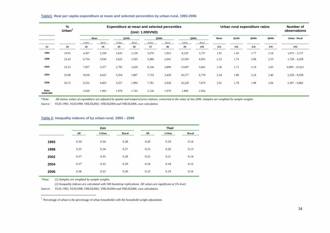
34

Table1: Real per capita expenditure at mean and selected percentiles by urban-rural, 1993-2006

% Urban1

Expenditure at mean and selected percentiles

(Unit: 1.000VND)

Urban rural expenditure ratios Number of observations

Mean Q10th Q50th Q90th Mean Q10th Q50th Q90th Urban - Rural

Urban Rural Urban Rural Urban Rural Urban Rural

(1) (2) (3) (4) (5) (6) (7) (8) (9) (10) (11) (12) (13) (14) (15)

1993 19.91 4,307 2,258 1,635 1,126 3,470 1,953 8,129 3,737 1.91 1.45 1.77 2.18 1,072 – 3,727

1998 22.43 6,754 3,030 2,622 1,503 5,486 2,641 12,503 4,935 2.23 1.74 2.08 2.53 1,730 – 4,269

2002 23.23 7,957 3,377 2,792 1,629 6,336 2,890 15,007 5,662 2.36 1.71 2.19 2.65 6,909 – 22,621

2004 25.80 9,018 4,025 3,354 1,807 7,719 3,450 16,277 6,778 2.24 1.86 2.24 2.40 2,250 – 6,938

2006 26.72 9,252 4,603 3,557 1,994 7,781 3,936 16,220 7,874 2.01 1.78 1.98 2.06 2,307 – 6,882

Ratio 2006/1993 2.029 1.993 1.978 1.743 2.136 1.979 1.898 2.056

*Note: All money values of expenditure are adjusted by spatial and temporal price indexes, converted to the value of Jan 2006. Samples are weighted by sample weights.

Source: VLSS 1993, VLSS1998, VHLSS2002, VHLSS2004 and VHLSS2006, own calculation.

Table 2 : Inequality indexes of by urban-rural, 1993 – 2006

Gini Theil

All Urban Rural All Urban Rural

1993 0.34 0.34 0.28 0.20 0.19 0.14

1998 0.35 0.34 0.27 0.23 0.20 0.13

2002 0.37 0.35 0.28 0.25 0.21 0.14

2004 0.37 0.33 0.29 0.24 0.18 0.15

2006 0.36 0.33 0.30 0.23 0.19 0.16

*Note: (1) Samples are weighted by sample weights.

(2) Inequality indexes are calculated with 500 bootstrap replications. All values are significant at 5% level.

Source: VLSS 1993, VLSS1998, VHLSS2002, VHLSS2004 and VHLSS2006, own calculation.

1 Percentage of urban is the percentage of urban households with the household weight adjustment.

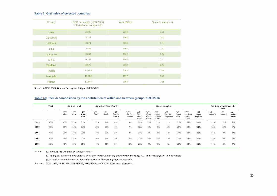
35

Table 3: Gini index of selected countries

Country GDP per capita (US$ 2005) international comparison

Year of Gini

Gini(consumption)

Laos 2,039 2002 0.35

Cambodia 2,727 2004 0.42

Vietnam 3,071 2004 0.37

India 3,452 2004 0.37

Indonesia 3,843 2002 0.34

China 6,757 2004 0.47

Thailand 8,677 2002 0.42

Russia 10,845 2002 0.40

Malaysia 10,882 1997 0.49

Poland 13,847 2002 0.35

Source: UNDP 2008, Human Development Report 2007/2008

Table 4a: Theil decomposition by the contribution of within and between groups, 1993-2006

Total By Urban-rural By region: North-South By seven regions Ethnicity of the household head

WT urban

WT rural

BT urban rural

WT North

WT South

BT North-South

WT Northern Uplands

WT Red River Delta

WT North Central Coast

WT South Central Coast

WT Central Highlands

WT South East

WT Mekong River Delta

BT seven

regions

WT majority

WT minority

BT major- minor

1993 100% 47% 32% 21% 31% 61% 8% 6% 22% 5% 12% 1% 21% 20% 12% 85% 13% 2%

1998 100% 35% 34% 31% 36% 60% 4% 7% 18% 8% 7% 2% 26% 14% 18% 83% 13% 4%

2002 100% 35% 32% 33% 41% 56% 3% 9% 23% 6% 6% 4% 24% 13% 16% 86% 8% 6%

2004 100% 35% 34% 31% 40% 57% 3% 10% 20% 6% 7% 4% 22% 14% 17% 85% 8% 7%

2006 100% 40% 35% 25% 44% 53% 3% 10% 23% 7% 6% 5% 22% 14% 13% 84% 8% 8%

*Note: (1) Samples are weighted by sample weights.

(2) All figures are calculated with 500 bootstrap replications using the method of Biewen (2002) and are significant at the 5% level.

(3)WT and BT are abbreviations for within-group and between-groups respectively.

Source: VLSS 1993, VLSS1998, VHLSS2002, VHLSS2004 and VHLSS2006, own calculation.

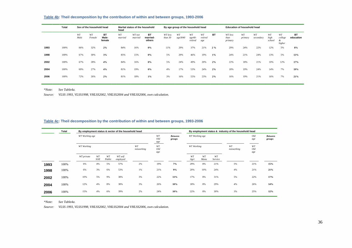
36

Table 4b : Theil decomposition by the contribution of within and between groups, 1993-2006

Total Sex of the household head Marital status of the household head By age group of the household head Education of household head

WT Male

WT Female

BT Male-

female WT

married WT not married

BT married- others

WT less than 30

WT age3040

WT age40-retired

WT retired age

BT WT less than primary

WT primary

WT secondary

WT high school

WT college & higher

BT education

1993 100% 66% 32% 2% 84% 16% 0% 11% 29% 37% 21% 2 % 29% 24% 22% 12% 5% 8%

1998 100% 67% 30% 3% 85% 15% 0% 5% 29% 46% 19% 1% 24% 21% 24% 13% 5% 13%

2002 100% 67% 28% 4% 84% 16% 0% 5% 24% 49% 20% 2% 22% 18% 21% 10% 12% 17%

2004 100% 69% 27% 4% 81% 19% 0% 4% 17% 53% 24% 2% 18% 19% 24% 14% 7% 19%

2006 100% 72% 26% 2% 81% 18% 1% 3% 16% 55% 23% 2% 16% 19% 21% 16% 7% 21%

*Note: See Table4a.

Source: VLSS 1993, VLSS1998, VHLSS2002, VHLSS2004 and VHLSS2006, own calculation.

Table 4c : Theil decomposition by the contribution of within and between groups, 1993-2006

Total By employment status & sector of the household head By employment status & industry of the household head

WT Working age WT Old age

Between groups

WT Working age Old age Between

groups

WT Working WT notworking

WT Old age

WT Working WT notworking

WT Old age

WT private WT SOE

WT Public

WT self employed WT

Agri WT

Manu WT

Service 1993 100% 6% 4% 5% 57% 2% 19% 7% 29% 8% 21% 5% 21% 15%

1998 100% 6% 3% 6% 53% 1% 21% 9% 20% 10% 24% 4% 21% 21%

2002 100% 10% 5% 9% 38% 3% 22% 13% 17% 8% 31% 5% 22% 17%

2004 100% 12% 4% 8% 38% 3% 26% 10% 18% 8% 29% 4% 26% 14%

2006 100% 15% 4% 6% 39% 2% 24% 10% 22% 8% 30% 3% 25% 12%

*Note: See Table4a.

Source: VLSS 1993, VLSS1998, VHLSS2002, VHLSS2004 and VHLSS2006, own calculation.

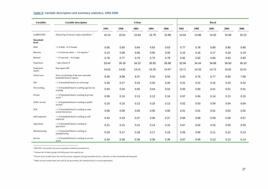
37

Table 5: Variable description and summary statistics, 1993 -2006

Variables Variable description Urban Rural

1993 1998 2002 2004 2006 1993 1998 2002 2004 2006

Ln(RPCEXP) Natural log of real per capita expenditure 2 15.15 15.61 15.64 15.79 15.86 14.54 14.88 14.92 15.09 15.22

Household head:

Male =1 if Male, =0 if Female 0.56 0.60 0.64 0.63 0.63 0.77 0.78 0.80 0.80 0.80

Minority = 1 if minority ethnic, = 0 if majority 3 0.10 0.08 0.06 0.06 0.06 0.15 0.16 0.17 0.18 0.19

Married = 1 if married, = 0 if single 0.78 0.77 0.79 0.79 0.78 0.82 0.82 0.83 0.82 0.83

Experience = age-schyear-6 33.64 35.18 34.22 35.92 35.88 32.94 34.44 34.86 36.50 36.33

Experience square

Exp square/100 14.02 14.81 14.21 15.25 14.97 13.71 14.33 14.72 15.81 15.51

School year Years of schooling of the more educated household head or spouse

8.48 8.96 9.37 9.43 9.55 6.40 6.76 6.77 6.95 7.06

Old = 1 if household head is at retired age 0.25 0.27 0.24 0.26 0.26 0.21 0.22 0.22 0.23 0.22

Not working = 1 if household head in working age but not working

0.03 0.03 0.05 0.04 0.02 0.00 0.00 0.01 0.01 0.01

Private = 1 if household head is working in private sector 4

0.09 0.10 0.13 0.12 0.16 0.07 0.06 0.14 0.13 0.15

Public servant = 1 if household head is working as public servant 5

0.10 0.10 0.13 0.16 0.13 0.02 0.03 0.04 0.04 0.04

SOE = 1 if household head is working in state owned enterprises

0.08 0.08 0.09 0.06 0.06 0.01 0.01 0.01 0.02 0.02

Self-employed = 1 if household head is working as self-employed

0.44 0.43 0.37 0.36 0.37 0.69 0.68 0.59 0.56 0.57

Agriculture = 1 if household head is working in agriculture

0.21 0.15 0.15 0.14 0.15 0.67 0.62 0.53 0.50 0.50

Manufacturing = 1 if household head is working in manufacturing

0.18 0.17 0.18 0.17 0.18 0.05 0.06 0.11 0.12 0.13

Service = 1 if household head is working in service sector

0.34 0.38 0.39 0.39 0.39 0.07 0.09 0.13 0.13 0.14

2 RPCEXP is household total yearly expenditure divided by household size.

3 Vietnam has 54 ethnic groups, the Kinh group is the majority one.

4 Private sector includes those who work for private companies, foreign investment sectors, collectives or other households and being paid.

5 Public servant includes those who work for the government, the communist party or social organizations.

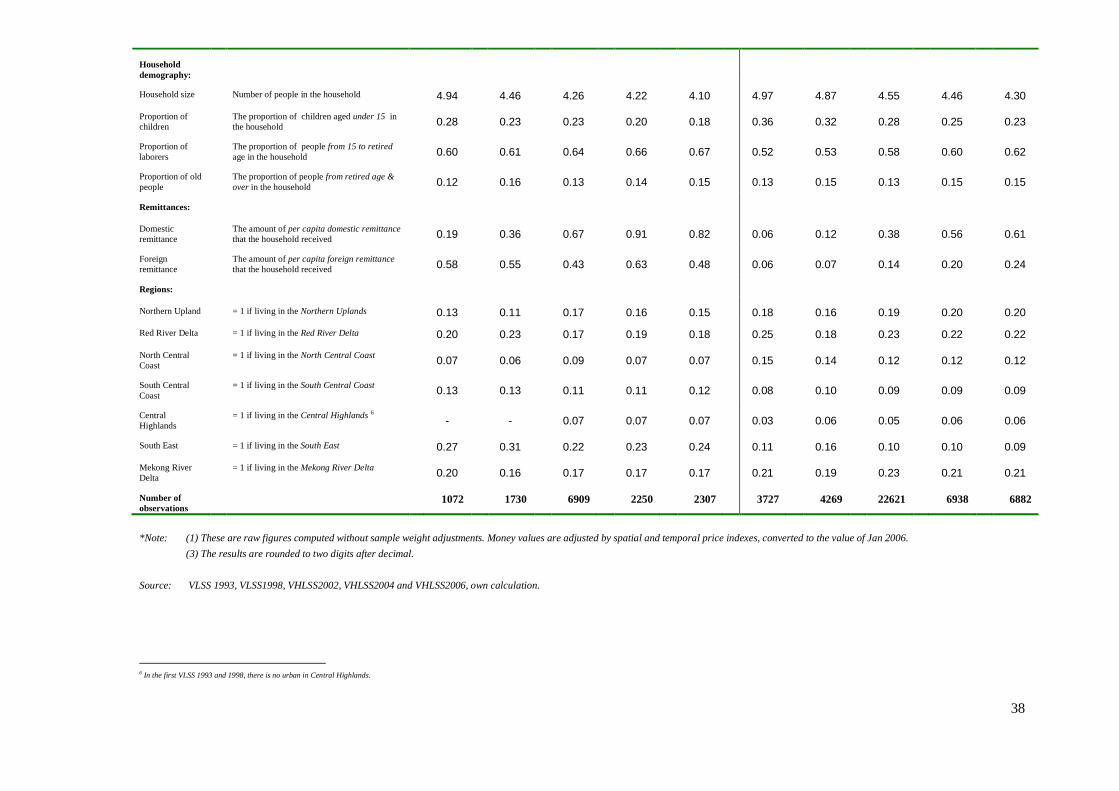
38

Household demography:

Household size Number of people in the household 4.94 4.46 4.26 4.22 4.10 4.97 4.87 4.55 4.46 4.30

Proportion of children

The proportion of children aged under 15 in the household

0.28 0.23 0.23 0.20 0.18 0.36 0.32 0.28 0.25 0.23

Proportion of laborers

The proportion of people from 15 to retired age in the household

0.60 0.61 0.64 0.66 0.67 0.52 0.53 0.58 0.60 0.62

Proportion of old people

The proportion of people from retired age & over in the household

0.12 0.16 0.13 0.14 0.15 0.13 0.15 0.13 0.15 0.15

Remittances:

Domestic remittance

The amount of per capita domestic remittance that the household received

0.19 0.36 0.67 0.91 0.82 0.06 0.12 0.38 0.56 0.61

Foreign remittance

The amount of per capita foreign remittance that the household received

0.58 0.55 0.43 0.63 0.48 0.06 0.07 0.14 0.20 0.24

Regions:

Northern Upland = 1 if living in the Northern Uplands 0.13 0.11 0.17 0.16 0.15 0.18 0.16 0.19 0.20 0.20

Red River Delta = 1 if living in the Red River Delta 0.20 0.23 0.17 0.19 0.18 0.25 0.18 0.23 0.22 0.22

North Central Coast

= 1 if living in the North Central Coast 0.07 0.06 0.09 0.07 0.07 0.15 0.14 0.12 0.12 0.12

South Central Coast

= 1 if living in the South Central Coast 0.13 0.13 0.11 0.11 0.12 0.08 0.10 0.09 0.09 0.09

Central Highlands

= 1 if living in the Central Highlands 6 - - 0.07 0.07 0.07 0.03 0.06 0.05 0.06 0.06

South East = 1 if living in the South East 0.27 0.31 0.22 0.23 0.24 0.11 0.16 0.10 0.10 0.09

Mekong River Delta

= 1 if living in the Mekong River Delta 0.20 0.16 0.17 0.17 0.17 0.21 0.19 0.23 0.21 0.21

Number of observations

1072 1730 6909 2250 2307 3727 4269 22621 6938 6882

*Note: (1) These are raw figures computed without sample weight adjustments. Money values are adjusted by spatial and temporal price indexes, converted to the value of Jan 2006.

(3) The results are rounded to two digits after decimal.

Source: VLSS 1993, VLSS1998, VHLSS2002, VHLSS2004 and VHLSS2006, own calculation.

6 In the first VLSS 1993 and 1998, there is no urban in Central Highlands.

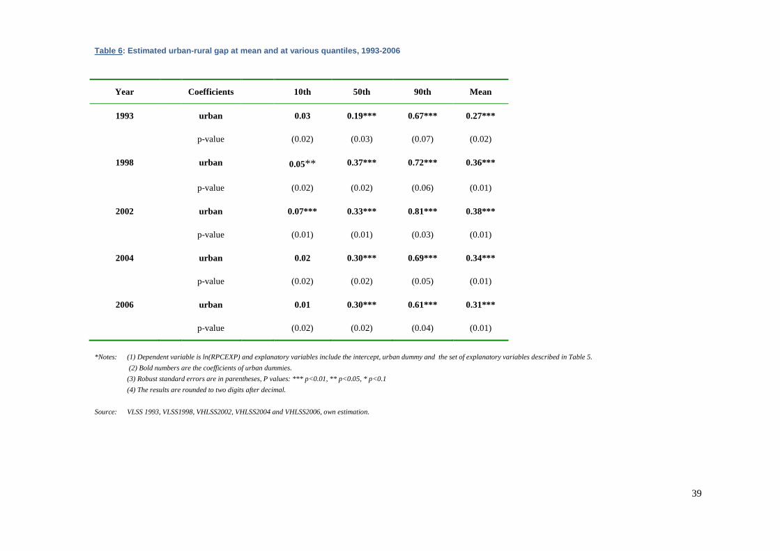
39

Table 6 : Estimated urban-rural gap at mean and at various quantiles, 1993-2006

Year Coefficients 10th 50th 90th Mean

1993 urban 0.03 0.19*** 0.67*** 0.27***

p-value (0.02) (0.03) (0.07) (0.02)

1998 urban 0.05** 0.37*** 0.72*** 0.36***

p-value (0.02) (0.02) (0.06) (0.01)

2002 urban 0.07*** 0.33*** 0.81*** 0.38***

p-value (0.01) (0.01) (0.03) (0.01)

2004 urban 0.02 0.30*** 0.69*** 0.34***

p-value (0.02) (0.02) (0.05) (0.01)

2006 urban 0.01 0.30*** 0.61*** 0.31***

p-value (0.02) (0.02) (0.04) (0.01)

*Notes: (1) Dependent variable is ln(RPCEXP) and explanatory variables include the intercept, urban dummy and the set of explanatory variables described in Table 5.

(2) Bold numbers are the coefficients of urban dummies.

(3) Robust standard errors are in parentheses, P values: *** p<0.01, ** p<0.05, * p<0.1

(4) The results are rounded to two digits after decimal.

Source: VLSS 1993, VLSS1998, VHLSS2002, VHLSS2004 and VHLSS2006, own estimation.

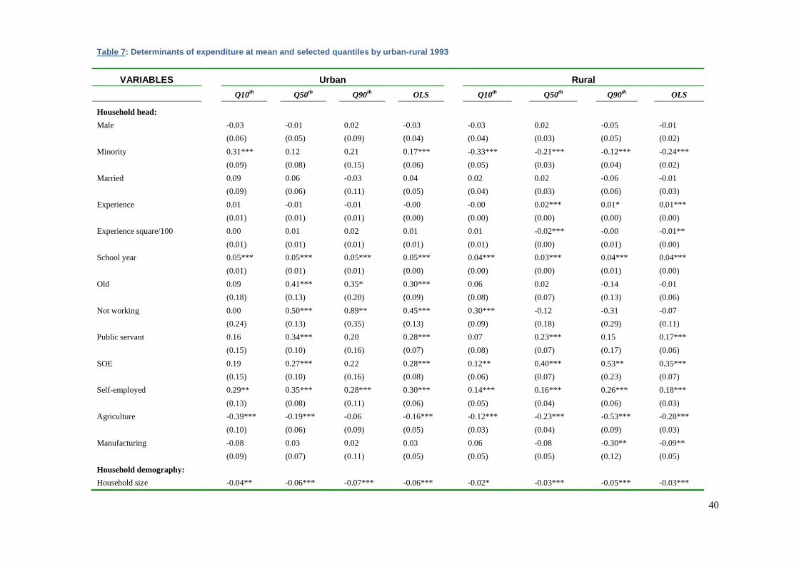
40

Table 7 : Determinants of expenditure at mean and selected quantiles by urban-rural 1993

VARIABLES Urban Rural

Q10th Q50th Q90th OLS Q10th Q50th Q90th OLS

Household head:

Male -0.03 -0.01 0.02 -0.03 -0.03 0.02 -0.05 -0.01

(0.06) (0.05) (0.09) (0.04) (0.04) (0.03) (0.05) (0.02)

Minority 0.31*** 0.12 0.21 0.17*** -0.33*** -0.21*** -0.12*** -0.24***

(0.09) (0.08) (0.15) (0.06) (0.05) (0.03) (0.04) (0.02)

Married 0.09 0.06 -0.03 0.04 0.02 0.02 -0.06 -0.01

(0.09) (0.06) (0.11) (0.05) (0.04) (0.03) (0.06) (0.03)

Experience 0.01 -0.01 -0.01 -0.00 -0.00 0.02*** 0.01* 0.01***

(0.01) (0.01) (0.01) (0.00) (0.00) (0.00) (0.00) (0.00)

Experience square/100 0.00 0.01 0.02 0.01 0.01 -0.02*** -0.00 -0.01**

(0.01) (0.01) (0.01) (0.01) (0.01) (0.00) (0.01) (0.00)

School year 0.05*** 0.05*** 0.05*** 0.05*** 0.04*** 0.03*** 0.04*** 0.04***

(0.01) (0.01) (0.01) (0.00) (0.00) (0.00) (0.01) (0.00)

Old 0.09 0.41*** 0.35* 0.30*** 0.06 0.02 -0.14 -0.01

(0.18) (0.13) (0.20) (0.09) (0.08) (0.07) (0.13) (0.06)

Not working 0.00 0.50*** 0.89** 0.45*** 0.30*** -0.12 -0.31 -0.07

(0.24) (0.13) (0.35) (0.13) (0.09) (0.18) (0.29) (0.11)

Public servant 0.16 0.34*** 0.20 0.28*** 0.07 0.23*** 0.15 0.17***

(0.15) (0.10) (0.16) (0.07) (0.08) (0.07) (0.17) (0.06)

SOE 0.19 0.27*** 0.22 0.28*** 0.12** 0.40*** 0.53** 0.35***

(0.15) (0.10) (0.16) (0.08) (0.06) (0.07) (0.23) (0.07)

Self-employed 0.29** 0.35*** 0.28*** 0.30*** 0.14*** 0.16*** 0.26*** 0.18***

(0.13) (0.08) (0.11) (0.06) (0.05) (0.04) (0.06) (0.03)

Agriculture -0.39*** -0.19*** -0.06 -0.16*** -0.12*** -0.23*** -0.53*** -0.28***

(0.10) (0.06) (0.09) (0.05) (0.03) (0.04) (0.09) (0.03)

Manufacturing -0.08 0.03 0.02 0.03 0.06 -0.08 -0.30** -0.09**

(0.09) (0.07) (0.11) (0.05) (0.05) (0.05) (0.12) (0.05)

Household demography:

Household size -0.04** -0.06*** -0.07*** -0.06*** -0.02* -0.03*** -0.05*** -0.03***

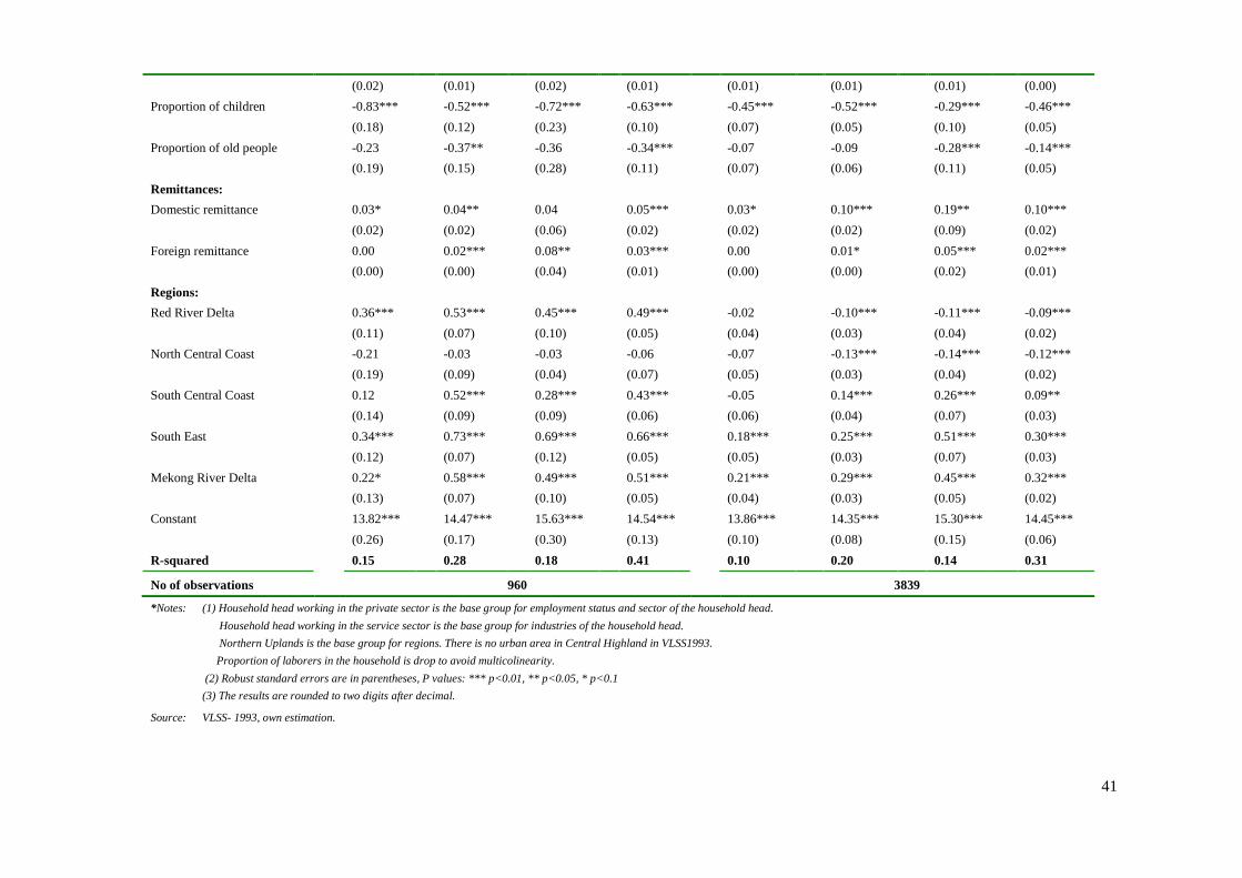
41

(0.02) (0.01) (0.02) (0.01) (0.01) (0.01) (0.01) (0.00)

Proportion of children -0.83*** -0.52*** -0.72*** -0.63*** -0.45*** -0.52*** -0.29*** -0.46***

(0.18) (0.12) (0.23) (0.10) (0.07) (0.05) (0.10) (0.05)

Proportion of old people -0.23 -0.37** -0.36 -0.34*** -0.07 -0.09 -0.28*** -0.14***

(0.19) (0.15) (0.28) (0.11) (0.07) (0.06) (0.11) (0.05)

Remittances:

Domestic remittance 0.03* 0.04** 0.04 0.05*** 0.03* 0.10*** 0.19** 0.10***

(0.02) (0.02) (0.06) (0.02) (0.02) (0.02) (0.09) (0.02)

Foreign remittance 0.00 0.02*** 0.08** 0.03*** 0.00 0.01* 0.05*** 0.02***

(0.00) (0.00) (0.04) (0.01) (0.00) (0.00) (0.02) (0.01)

Regions:

Red River Delta 0.36*** 0.53*** 0.45*** 0.49*** -0.02 -0.10*** -0.11*** -0.09***

(0.11) (0.07) (0.10) (0.05) (0.04) (0.03) (0.04) (0.02)

North Central Coast -0.21 -0.03 -0.03 -0.06 -0.07 -0.13*** -0.14*** -0.12***

(0.19) (0.09) (0.04) (0.07) (0.05) (0.03) (0.04) (0.02)

South Central Coast 0.12 0.52*** 0.28*** 0.43*** -0.05 0.14*** 0.26*** 0.09**

(0.14) (0.09) (0.09) (0.06) (0.06) (0.04) (0.07) (0.03)

South East 0.34*** 0.73*** 0.69*** 0.66*** 0.18*** 0.25*** 0.51*** 0.30***

(0.12) (0.07) (0.12) (0.05) (0.05) (0.03) (0.07) (0.03)

Mekong River Delta 0.22* 0.58*** 0.49*** 0.51*** 0.21*** 0.29*** 0.45*** 0.32***

(0.13) (0.07) (0.10) (0.05) (0.04) (0.03) (0.05) (0.02)

Constant 13.82*** 14.47*** 15.63*** 14.54*** 13.86*** 14.35*** 15.30*** 14.45***

(0.26) (0.17) (0.30) (0.13) (0.10) (0.08) (0.15) (0.06)

R-squared 0.15 0.28 0.18 0.41 0.10 0.20 0.14 0.31

No of observations 960 3839

*Notes: (1) Household head working in the private sector is the base group for employment status and sector of the household head.

Household head working in the service sector is the base group for industries of the household head.

Northern Uplands is the base group for regions. There is no urban area in Central Highland in VLSS1993.

Proportion of laborers in the household is drop to avoid multicolinearity.

(2) Robust standard errors are in parentheses, P values: *** p<0.01, ** p<0.05, * p<0.1

(3) The results are rounded to two digits after decimal.

Source: VLSS- 1993, own estimation.

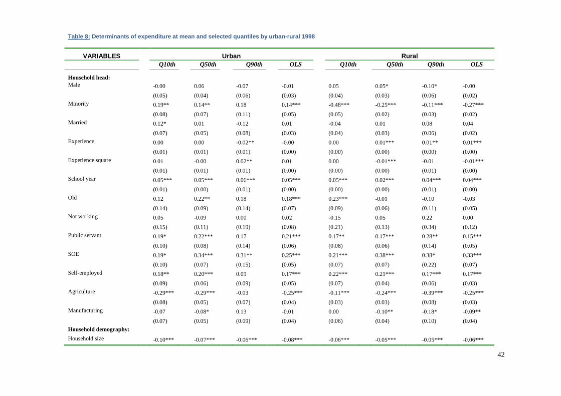
42

Table 8: Determinants of expenditure at mean and selected q uantiles by urban-rural 1998

VARIABLES Urban Rural Q10th Q50th Q90th OLS Q10th Q50th Q90th OLS

Household head:

Male -0.00 0.06 -0.07 -0.01 0.05 0.05* -0.10* -0.00

(0.05) (0.04) (0.06) (0.03) (0.04) (0.03) (0.06) (0.02)

Minority 0.19** 0.14** 0.18 0.14*** -0.48*** -0.25*** -0.11*** -0.27***

(0.08) (0.07) (0.11) (0.05) (0.05) (0.02) (0.03) (0.02) Married 0.12* 0.01 -0.12 0.01 -0.04 0.01 0.08 0.04

(0.07) (0.05) (0.08) (0.03) (0.04) (0.03) (0.06) (0.02)

Experience 0.00 0.00 -0.02** -0.00 0.00 0.01*** 0.01** 0.01***

(0.01) (0.01) (0.01) (0.00) (0.00) (0.00) (0.00) (0.00)

Experience square 0.01 -0.00 0.02** 0.01 0.00 -0.01*** -0.01 -0.01*** (0.01) (0.01) (0.01) (0.00) (0.00) (0.00) (0.01) (0.00)

School year 0.05*** 0.05*** 0.06*** 0.05*** 0.05*** 0.02** * 0.04*** 0.04***

(0.01) (0.00) (0.01) (0.00) (0.00) (0.00) (0.01) (0.00)

Old 0.12 0.22** 0.18 0.18*** 0.23*** -0.01 -0.10 -0.03

(0.14) (0.09) (0.14) (0.07) (0.09) (0.06) (0.11) (0.05)

Not working 0.05 -0.09 0.00 0.02 -0.15 0.05 0.22 0.00 (0.15) (0.11) (0.19) (0.08) (0.21) (0.13) (0.34) (0.12)

Public servant 0.19* 0.22*** 0.17 0.21*** 0.17** 0.17*** 0.28** 0.15***

(0.10) (0.08) (0.14) (0.06) (0.08) (0.06) (0.14) (0.05)

SOE 0.19* 0.34*** 0.31** 0.25*** 0.21*** 0.38*** 0.38* 0.33***

(0.10) (0.07) (0.15) (0.05) (0.07) (0.07) (0.22) (0.07)

Self-employed 0.18** 0.20*** 0.09 0.17*** 0.22*** 0.21*** 0.17*** 0.17***

(0.09) (0.06) (0.09) (0.05) (0.07) (0.04) (0.06) (0.03)

Agriculture -0.29*** -0.29*** -0.03 -0.25*** -0.11*** -0.24*** -0.39*** -0.25***

(0.08) (0.05) (0.07) (0.04) (0.03) (0.03) (0.08) (0.03)

Manufacturing -0.07 -0.08* 0.13 -0.01 0.00 -0.10** -0.18* -0.09**

(0.07) (0.05) (0.09) (0.04) (0.06) (0.04) (0.10) (0.04)

Household demography: Household size -0.10*** -0.07*** -0.06*** -0.08*** -0.06*** - 0.05*** -0.05*** -0.06***

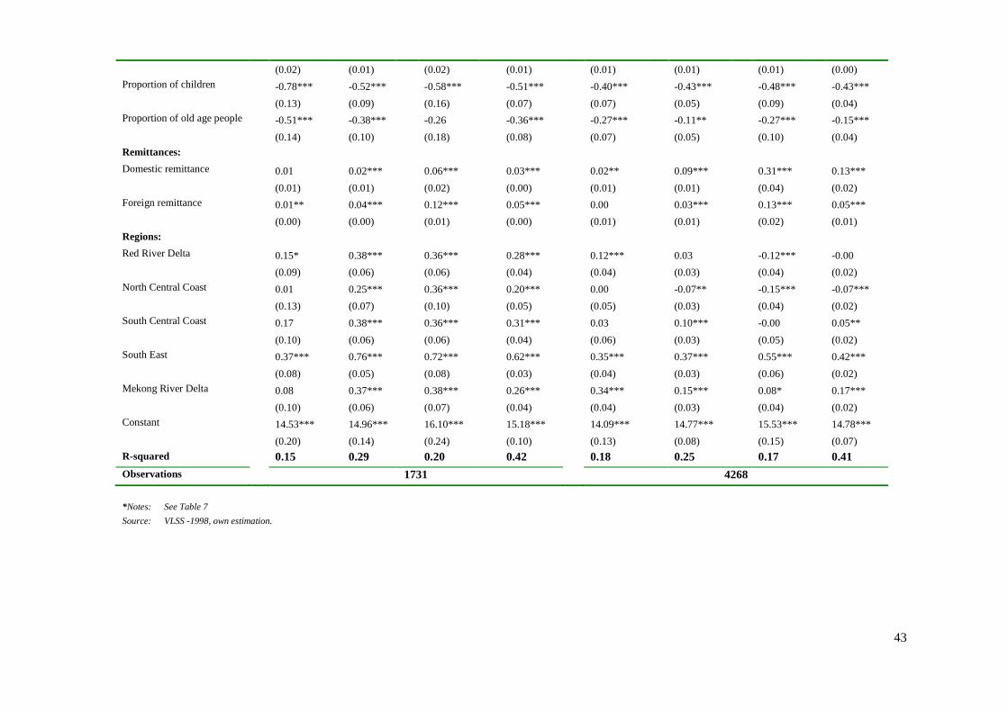
43

(0.02) (0.01) (0.02) (0.01) (0.01) (0.01) (0.01) (0.00)

Proportion of children -0.78*** -0.52*** -0.58*** -0.51*** -0.40*** - 0.43*** -0.48*** -0.43***

(0.13) (0.09) (0.16) (0.07) (0.07) (0.05) (0.09) (0.04) Proportion of old age people -0.51*** -0.38*** -0.26 -0.36*** -0.27*** -0.11** -0.27*** -0.15***

(0.14) (0.10) (0.18) (0.08) (0.07) (0.05) (0.10) (0.04)

Remittances:

Domestic remittance 0.01 0.02*** 0.06*** 0.03*** 0.02** 0.09*** 0.31*** 0.13***

(0.01) (0.01) (0.02) (0.00) (0.01) (0.01) (0.04) (0.02)

Foreign remittance 0.01** 0.04*** 0.12*** 0.05*** 0.00 0.03*** 0.13*** 0.05***

(0.00) (0.00) (0.01) (0.00) (0.01) (0.01) (0.02) (0.01)

Regions:

Red River Delta 0.15* 0.38*** 0.36*** 0.28*** 0.12*** 0.03 -0.12*** -0.00

(0.09) (0.06) (0.06) (0.04) (0.04) (0.03) (0.04) (0.02)

North Central Coast 0.01 0.25*** 0.36*** 0.20*** 0.00 -0.07** -0.15*** -0.07*** (0.13) (0.07) (0.10) (0.05) (0.05) (0.03) (0.04) (0.02)

South Central Coast 0.17 0.38*** 0.36*** 0.31*** 0.03 0.10*** -0.00 0.05**

(0.10) (0.06) (0.06) (0.04) (0.06) (0.03) (0.05) (0.02)

South East 0.37*** 0.76*** 0.72*** 0.62*** 0.35*** 0.37** * 0.55*** 0.42***

(0.08) (0.05) (0.08) (0.03) (0.04) (0.03) (0.06) (0.02)

Mekong River Delta 0.08 0.37*** 0.38*** 0.26*** 0.34*** 0.15*** 0.08* 0.17*** (0.10) (0.06) (0.07) (0.04) (0.04) (0.03) (0.04) (0.02)

Constant 14.53*** 14.96*** 16.10*** 15.18*** 14.09*** 14.77*** 15.53*** 14.78***

(0.20) (0.14) (0.24) (0.10) (0.13) (0.08) (0.15) (0.07)

R-squared 0.15 0.29 0.20 0.42 0.18 0.25 0.17 0.41

Observations 1731 4268

*Notes: See Table 7

Source: VLSS -1998, own estimation.

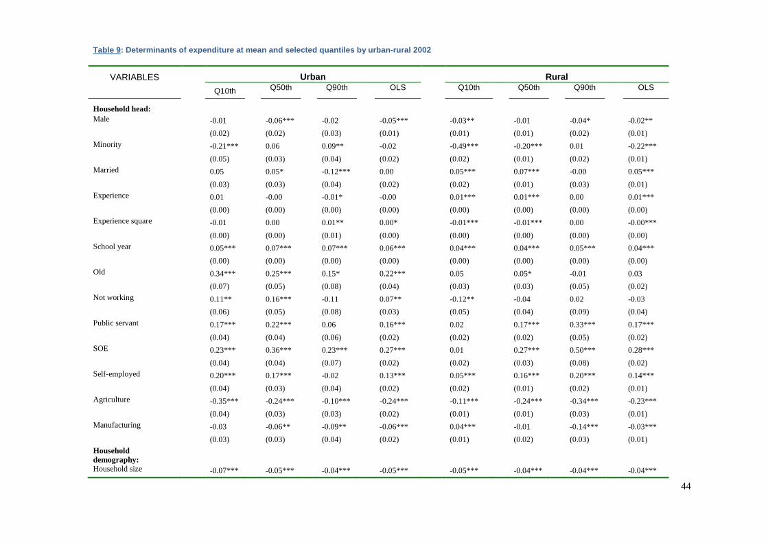
44

Table 9 : Determinants of expenditure at mean and selected quantiles by urban-rural 2002

VARIABLES Urban Rural

Q10th Q50th Q90th OLS Q10th Q50th Q90th OLS

Household head: Male -0.01 -0.06*** -0.02 -0.05*** -0.03** -0.01 -0.04* -0.02** (0.02) (0.02) (0.03) (0.01) (0.01) (0.01) (0.02) (0.01) Minority -0.21*** 0.06 0.09** -0.02 -0.49*** -0.20*** 0.01 -0.22*** (0.05) (0.03) (0.04) (0.02) (0.02) (0.01) (0.02) (0.01) Married 0.05 0.05* -0.12*** 0.00 0.05*** 0.07*** -0.00 0.05***

(0.03) (0.03) (0.04) (0.02) (0.02) (0.01) (0.03) (0.01) Experience 0.01 -0.00 -0.01* -0.00 0.01*** 0.01*** 0.00 0.01*** (0.00) (0.00) (0.00) (0.00) (0.00) (0.00) (0.00) (0.00) Experience square -0.01 0.00 0.01** 0.00* -0.01*** -0.01*** 0.00 -0.00*** (0.00) (0.00) (0.01) (0.00) (0.00) (0.00) (0.00) (0.00) School year 0.05*** 0.07*** 0.07*** 0.06*** 0.04*** 0.04* ** 0.05*** 0.04*** (0.00) (0.00) (0.00) (0.00) (0.00) (0.00) (0.00) (0.00) Old 0.34*** 0.25*** 0.15* 0.22*** 0.05 0.05* -0.01 0.03 (0.07) (0.05) (0.08) (0.04) (0.03) (0.03) (0.05) (0.02) Not working 0.11** 0.16*** -0.11 0.07** -0.12** -0.04 0.02 -0.03 (0.06) (0.05) (0.08) (0.03) (0.05) (0.04) (0.09) (0.04)

Public servant 0.17*** 0.22*** 0.06 0.16*** 0.02 0.17*** 0.33*** 0.17*** (0.04) (0.04) (0.06) (0.02) (0.02) (0.02) (0.05) (0.02) SOE 0.23*** 0.36*** 0.23*** 0.27*** 0.01 0.27*** 0.50*** 0.28*** (0.04) (0.04) (0.07) (0.02) (0.02) (0.03) (0.08) (0.02) Self-employed 0.20*** 0.17*** -0.02 0.13*** 0.05*** 0.16*** 0.20*** 0.14***

(0.04) (0.03) (0.04) (0.02) (0.02) (0.01) (0.02) (0.01) Agriculture -0.35*** -0.24*** -0.10*** -0.24*** -0.11*** -0.24*** -0.34*** -0.23*** (0.04) (0.03) (0.03) (0.02) (0.01) (0.01) (0.03) (0.01) Manufacturing -0.03 -0.06** -0.09** -0.06*** 0.04*** -0.01 -0.14*** -0.03*** (0.03) (0.03) (0.04) (0.02) (0.01) (0.02) (0.03) (0.01)

Household demography:

Household size -0.07*** -0.05*** -0.04*** -0.05*** -0.05*** -0.04*** -0.04*** -0.04***

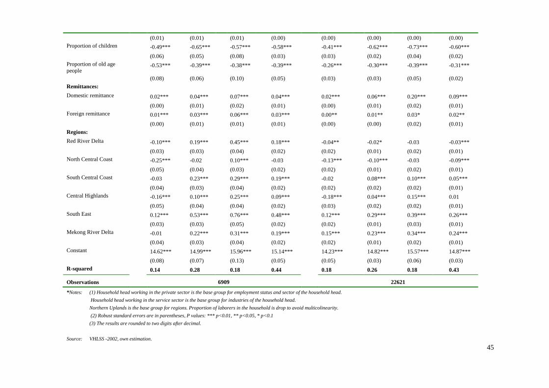
45

(0.01) (0.01) (0.01) (0.00) (0.00) (0.00) (0.00) (0.00) Proportion of children -0.49*** -0.65*** -0.57*** -0.58*** -0.41*** -0.62*** -0.73*** -0.60*** (0.06) (0.05) (0.08) (0.03) (0.03) (0.02) (0.04) (0.02) Proportion of old age people

-0.53*** -0.39*** -0.38*** -0.39*** -0.26*** -0.30*** -0.39*** -0.31***

(0.08) (0.06) (0.10) (0.05) (0.03) (0.03) (0.05) (0.02)

Remittances: Domestic remittance 0.02*** 0.04*** 0.07*** 0.04*** 0.02*** 0.06* ** 0.20*** 0.09*** (0.00) (0.01) (0.02) (0.01) (0.00) (0.01) (0.02) (0.01) Foreign remittance 0.01*** 0.03*** 0.06*** 0.03*** 0.00** 0.01** 0.03* 0.02** (0.00) (0.01) (0.01) (0.01) (0.00) (0.00) (0.02) (0.01)

Regions: Red River Delta -0.10*** 0.19*** 0.45*** 0.18*** -0.04** -0.02* -0.03 -0.03*** (0.03) (0.03) (0.04) (0.02) (0.02) (0.01) (0.02) (0.01) North Central Coast -0.25*** -0.02 0.10*** -0.03 -0.13*** -0.10*** -0.03 -0.09*** (0.05) (0.04) (0.03) (0.02) (0.02) (0.01) (0.02) (0.01) South Central Coast -0.03 0.23*** 0.29*** 0.19*** -0.02 0.08*** 0.10*** 0.05*** (0.04) (0.03) (0.04) (0.02) (0.02) (0.02) (0.02) (0.01) Central Highlands -0.16*** 0.10*** 0.25*** 0.09*** -0.18*** 0.0 4*** 0.15*** 0.01 (0.05) (0.04) (0.04) (0.02) (0.03) (0.02) (0.02) (0.01)

South East 0.12*** 0.53*** 0.76*** 0.48*** 0.12*** 0.29* ** 0.39*** 0.26*** (0.03) (0.03) (0.05) (0.02) (0.02) (0.01) (0.03) (0.01) Mekong River Delta -0.01 0.22*** 0.31*** 0.19*** 0.15*** 0.23*** 0.34*** 0.24*** (0.04) (0.03) (0.04) (0.02) (0.02) (0.01) (0.02) (0.01) Constant 14.62*** 14.99*** 15.96*** 15.14*** 14.23*** 14.82*** 15.57*** 14.87***

(0.08) (0.07) (0.13) (0.05) (0.05) (0.03) (0.06) (0.03)

R-squared 0.14 0.28 0.18 0.44 0.18 0.26 0.18 0.43

Observations 6909 22621

*Notes: (1) Household head working in the private sector is the base group for employment status and sector of the household head.

Household head working in the service sector is the base group for industries of the household head.

Northern Uplands is the base group for regions. Proportion of laborers in the household is drop to avoid multicolinearity.

(2) Robust standard errors are in parentheses, P values: *** p<0.01, ** p<0.05, * p<0.1

(3) The results are rounded to two digits after decimal.

Source: VHLSS -2002, own estimation.

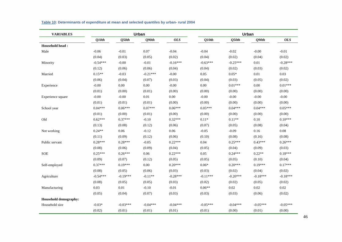
46

Table 10: Determinants of expenditure at mean and selected quantiles by urban- rural 2004

VARIABLES Urban Urban

Q10th Q50th Q90th OLS Q10th Q50th Q90th OLS

Household head :

Male -0.06 -0.01 0.07 -0.04 -0.04 -0.02 -0.00 -0.01

(0.04) (0.03) (0.05) (0.02) (0.04) (0.02) (0.04) (0.02)

Minority -0.54*** -0.00 -0.01 -0.16*** -0.63*** -0.25*** 0.01 -0.28***

(0.12) (0.06) (0.06) (0.04) (0.04) (0.02) (0.03) (0.02)

Married 0.15** -0.03 -0.21*** -0.00 0.05 0.05* 0.01 0.03

(0.06) (0.04) (0.07) (0.03) (0.04) (0.03) (0.05) (0.02)

Experience -0.00 0.00 0.00 -0.00 0.00 0.01*** 0.00 0.01***

(0.01) (0.00) (0.01) (0.00) (0.00) (0.00) (0.00) (0.00)

Experience square -0.00 -0.00 0.01 0.00 -0.00 -0.00 -0.00 -0.00

(0.01) (0.01) (0.01) (0.00) (0.00) (0.00) (0.00) (0.00)

School year 0.04*** 0.06*** 0.07*** 0.06*** 0.05*** 0.04*** 0.04*** 0.05***

(0.01) (0.00) (0.01) (0.00) (0.00) (0.00) (0.00) (0.00)

Old 0.62*** 0.37*** -0.10 0.32*** 0.11* 0.11** 0.10 0.10***

(0.13) (0.08) (0.12) (0.06) (0.07) (0.05) (0.08) (0.04)

Not working 0.24** 0.06 -0.12 0.06 -0.05 -0.09 0.16 0.08

(0.11) (0.09) (0.12) (0.06) (0.10) (0.08) (0.16) (0.08)

Public servant 0.28*** 0.28*** -0.05 0.22*** 0.04 0.25*** 0.43*** 0.26***

(0.08) (0.06) (0.09) (0.04) (0.05) (0.04) (0.09) (0.03)

SOE 0.25*** 0.26*** 0.06 0.22*** 0.05 0.24*** 0.22** 0.18***

(0.09) (0.07) (0.12) (0.05) (0.05) (0.05) (0.10) (0.04)

Self-employed 0.37*** 0.19*** 0.00 0.20*** 0.06* 0.20*** 0.19*** 0.17***

(0.08) (0.05) (0.06) (0.03) (0.03) (0.02) (0.04) (0.02)

Agriculture -0.54*** -0.19*** -0.11** -0.28*** -0.11*** -0.20*** -0.18*** -0.18***

(0.08) (0.05) (0.05) (0.03) (0.02) (0.02) (0.05) (0.02)

Manufacturing 0.03 0.01 -0.10 -0.01 0.06** 0.02 0.02 0.02

(0.05) (0.04) (0.07) (0.03) (0.03) (0.03) (0.06) (0.02)

Household demography:

Household size -0.03* -0.03*** -0.04*** -0.04*** -0.05*** -0.04*** -0.05*** -0.05***

(0.02) (0.01) (0.01) (0.01) (0.01) (0.00) (0.01) (0.00)

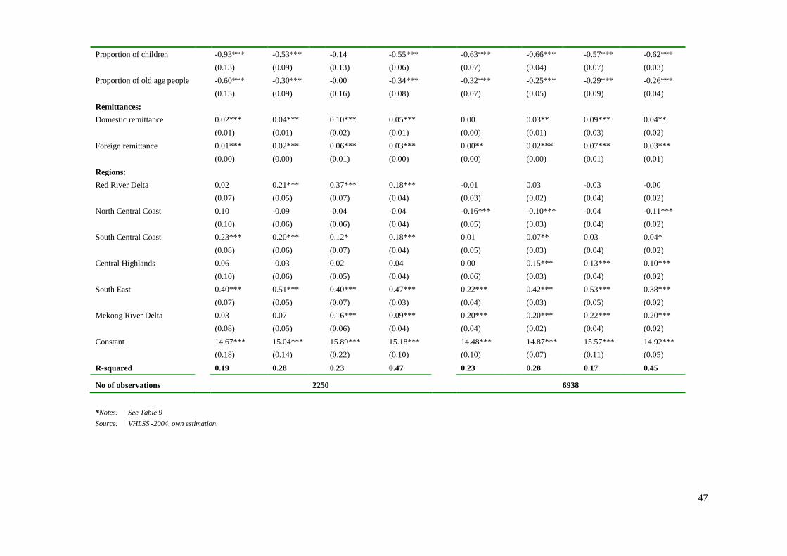
47

Proportion of children -0.93*** -0.53*** -0.14 -0.55*** -0.63*** -0.66*** -0.57*** -0.62***

(0.13) (0.09) (0.13) (0.06) (0.07) (0.04) (0.07) (0.03)

Proportion of old age people -0.60*** -0.30*** -0.00 -0.34*** -0.32*** -0.25*** -0.29*** -0.26***

(0.15) (0.09) (0.16) (0.08) (0.07) (0.05) (0.09) (0.04)

Remittances:

Domestic remittance 0.02*** 0.04*** 0.10*** 0.05*** 0.00 0.03** 0.09*** 0.04**

(0.01) (0.01) (0.02) (0.01) (0.00) (0.01) (0.03) (0.02)

Foreign remittance 0.01*** 0.02*** 0.06*** 0.03*** 0.00** 0.02*** 0.07*** 0.03***

(0.00) (0.00) (0.01) (0.00) (0.00) (0.00) (0.01) (0.01)

Regions:

Red River Delta 0.02 0.21*** 0.37*** 0.18*** -0.01 0.03 -0.03 -0.00

(0.07) (0.05) (0.07) (0.04) (0.03) (0.02) (0.04) (0.02)

North Central Coast 0.10 -0.09 -0.04 -0.04 -0.16*** -0.10*** -0.04 -0.11***

(0.10) (0.06) (0.06) (0.04) (0.05) (0.03) (0.04) (0.02)

South Central Coast 0.23*** 0.20*** 0.12* 0.18*** 0.01 0.07** 0.03 0.04*

(0.08) (0.06) (0.07) (0.04) (0.05) (0.03) (0.04) (0.02)

Central Highlands 0.06 -0.03 0.02 0.04 0.00 0.15*** 0.13*** 0.10***

(0.10) (0.06) (0.05) (0.04) (0.06) (0.03) (0.04) (0.02)

South East 0.40*** 0.51*** 0.40*** 0.47*** 0.22*** 0.42*** 0.53*** 0.38***

(0.07) (0.05) (0.07) (0.03) (0.04) (0.03) (0.05) (0.02)

Mekong River Delta 0.03 0.07 0.16*** 0.09*** 0.20*** 0.20*** 0.22*** 0.20***

(0.08) (0.05) (0.06) (0.04) (0.04) (0.02) (0.04) (0.02)

Constant 14.67*** 15.04*** 15.89*** 15.18*** 14.48*** 14.87*** 15.57*** 14.92***

(0.18) (0.14) (0.22) (0.10) (0.10) (0.07) (0.11) (0.05)

R-squared 0.19 0.28 0.23 0.47 0.23 0.28 0.17 0.45

No of observations 2250 6938

*Notes: See Table 9

Source: VHLSS -2004, own estimation.

48

Table 11: Determinants of expenditure at mean and selected quantiles by urban-rural 2006

VARIABLES Urban Rural

Q10th Q50th Q90th OLS Q10th Q50th Q90th OLS

Household head:

Male -0.03 0.03 0.08 0.01 0.02 0.02 -0.01 0.01

(0.04) (0.03) (0.05) (0.02) (0.03) (0.02) (0.05) (0.02)

Minority -0.34*** -0.01 0.08 -0.07 -0.55*** -0.27*** -0.08*** -0.29***

(0.12) (0.05) (0.07) (0.04) (0.04) (0.02) (0.03) (0.02)

Married 0.15** 0.06 -0.14** 0.01 0.07* 0.08*** 0.04 0.06***

(0.07) (0.04) (0.07) (0.03) (0.04) (0.03) (0.05) (0.02)

Experience -0.00 0.00 -0.00 -0.00 0.00 0.01*** 0.00 0.00***

(0.01) (0.00) (0.01) (0.00) (0.00) (0.00) (0.00) (0.00)

Experience square -0.01 -0.01 -0.00 -0.00 -0.00 -0.01*** -0.01 -0.01***

(0.01) (0.00) (0.01) (0.00) (0.00) (0.00) (0.00) (0.00)

School year 0.08*** 0.06*** 0.06*** 0.07*** 0.06*** 0.04*** 0.04*** 0.04***

(0.01) (0.00) (0.01) (0.00) (0.00) (0.00) (0.00) (0.00)

Old 0.39*** 0.11 -0.07 0.13** 0.02 0.08 0.18** 0.05

(0.13) (0.07) (0.12) (0.06) (0.06) (0.05) (0.07) (0.03)

Not working 0.15 0.15 0.03 0.05 -0.08 0.00 0.17 -0.06

(0.15) (0.10) (0.19) (0.09) (0.11) (0.09) (0.20) (0.09)

Public servant 0.11 0.22*** -0.06 0.14*** 0.02 0.32*** 0.62*** 0.32***

(0.08) (0.05) (0.10) (0.04) (0.05) (0.04) (0.10) (0.03)

SOE 0.25*** 0.31*** 0.17 0.26*** 0.10* 0.24*** 0.44*** 0.24***

(0.09) (0.06) (0.12) (0.04) (0.05) (0.05) (0.11) (0.04)

Self employed 0.28*** 0.06 -0.18*** 0.08** 0.11*** 0.24*** 0.20*** 0.18***

(0.08) (0.04) (0.06) (0.03) (0.03) (0.03) (0.03) (0.02)

Agriculture -0.44*** -0.18*** -0.07 -0.23*** -0.12*** -0.24*** -0.11*** -0.19***

(0.08) (0.04) (0.05) (0.03) (0.02) (0.02) (0.04) (0.02)

Manufacturing -0.11* -0.14*** -0.15** -0.10*** 0.07** 0.00 0.06 0.01

(0.06) (0.04) (0.06) (0.03) (0.03) (0.03) (0.06) (0.02)

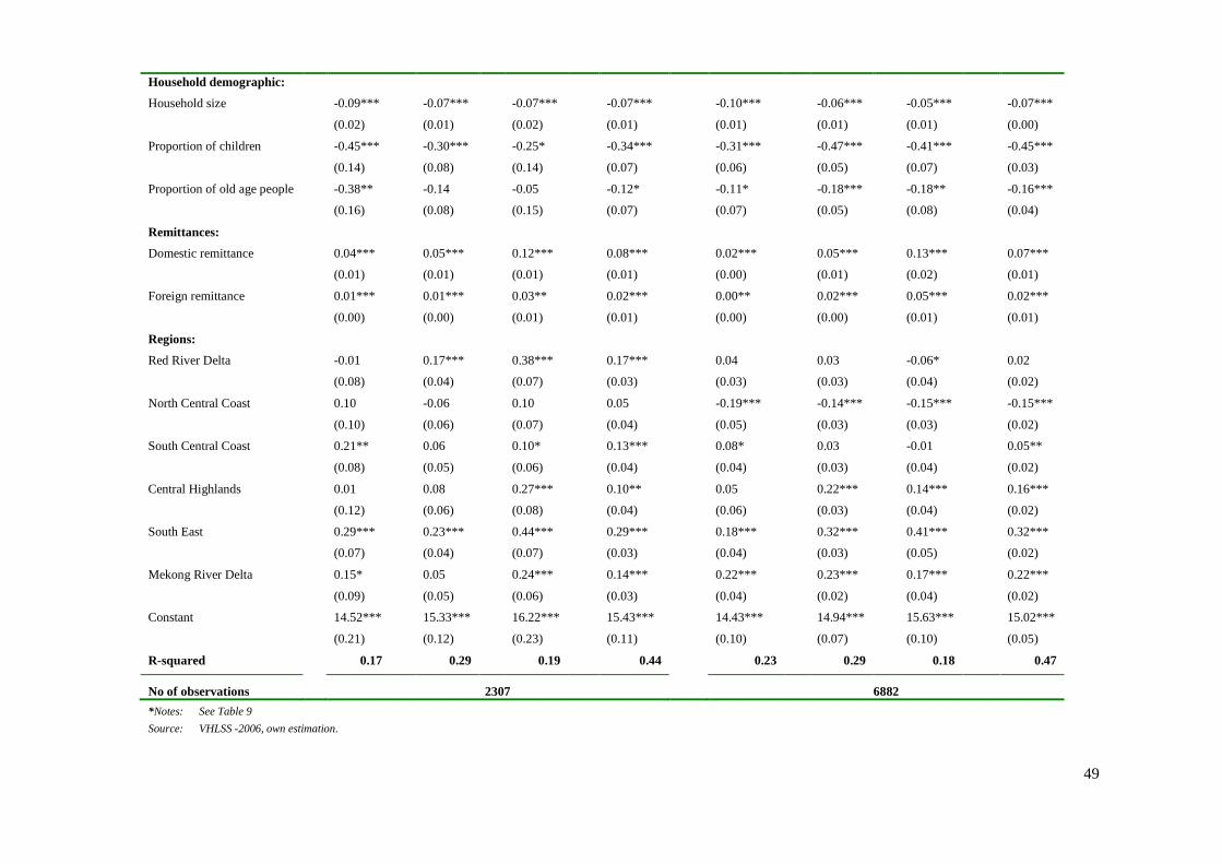
49

Household demographic:

Household size -0.09*** -0.07*** -0.07*** -0.07*** -0.10*** -0.06*** -0.05*** -0.07***

(0.02) (0.01) (0.02) (0.01) (0.01) (0.01) (0.01) (0.00)

Proportion of children -0.45*** -0.30*** -0.25* -0.34*** -0.31*** -0.47*** -0.41*** -0.45***

(0.14) (0.08) (0.14) (0.07) (0.06) (0.05) (0.07) (0.03)

Proportion of old age people -0.38** -0.14 -0.05 -0.12* -0.11* -0.18*** -0.18** -0.16***

(0.16) (0.08) (0.15) (0.07) (0.07) (0.05) (0.08) (0.04)

Remittances:

Domestic remittance 0.04*** 0.05*** 0.12*** 0.08*** 0.02*** 0.05*** 0.13*** 0.07***

(0.01) (0.01) (0.01) (0.01) (0.00) (0.01) (0.02) (0.01)

Foreign remittance 0.01*** 0.01*** 0.03** 0.02*** 0.00** 0.02*** 0.05*** 0.02***

(0.00) (0.00) (0.01) (0.01) (0.00) (0.00) (0.01) (0.01)

Regions:

Red River Delta -0.01 0.17*** 0.38*** 0.17*** 0.04 0.03 -0.06* 0.02

(0.08) (0.04) (0.07) (0.03) (0.03) (0.03) (0.04) (0.02)

North Central Coast 0.10 -0.06 0.10 0.05 -0.19*** -0.14*** -0.15*** -0.15***

(0.10) (0.06) (0.07) (0.04) (0.05) (0.03) (0.03) (0.02)

South Central Coast 0.21** 0.06 0.10* 0.13*** 0.08* 0.03 -0.01 0.05**

(0.08) (0.05) (0.06) (0.04) (0.04) (0.03) (0.04) (0.02)

Central Highlands 0.01 0.08 0.27*** 0.10** 0.05 0.22*** 0.14*** 0.16***

(0.12) (0.06) (0.08) (0.04) (0.06) (0.03) (0.04) (0.02)

South East 0.29*** 0.23*** 0.44*** 0.29*** 0.18*** 0.32*** 0.41*** 0.32***

(0.07) (0.04) (0.07) (0.03) (0.04) (0.03) (0.05) (0.02)

Mekong River Delta 0.15* 0.05 0.24*** 0.14*** 0.22*** 0.23*** 0.17*** 0.22***

(0.09) (0.05) (0.06) (0.03) (0.04) (0.02) (0.04) (0.02)

Constant 14.52*** 15.33*** 16.22*** 15.43*** 14.43*** 14.94*** 15.63*** 15.02***

(0.21) (0.12) (0.23) (0.11) (0.10) (0.07) (0.10) (0.05)

R-squared 0.17 0.29 0.19 0.44 0.23 0.29 0.18 0.47

No of observations 2307 6882

*Notes: See Table 9

Source: VHLSS -2006, own estimation.

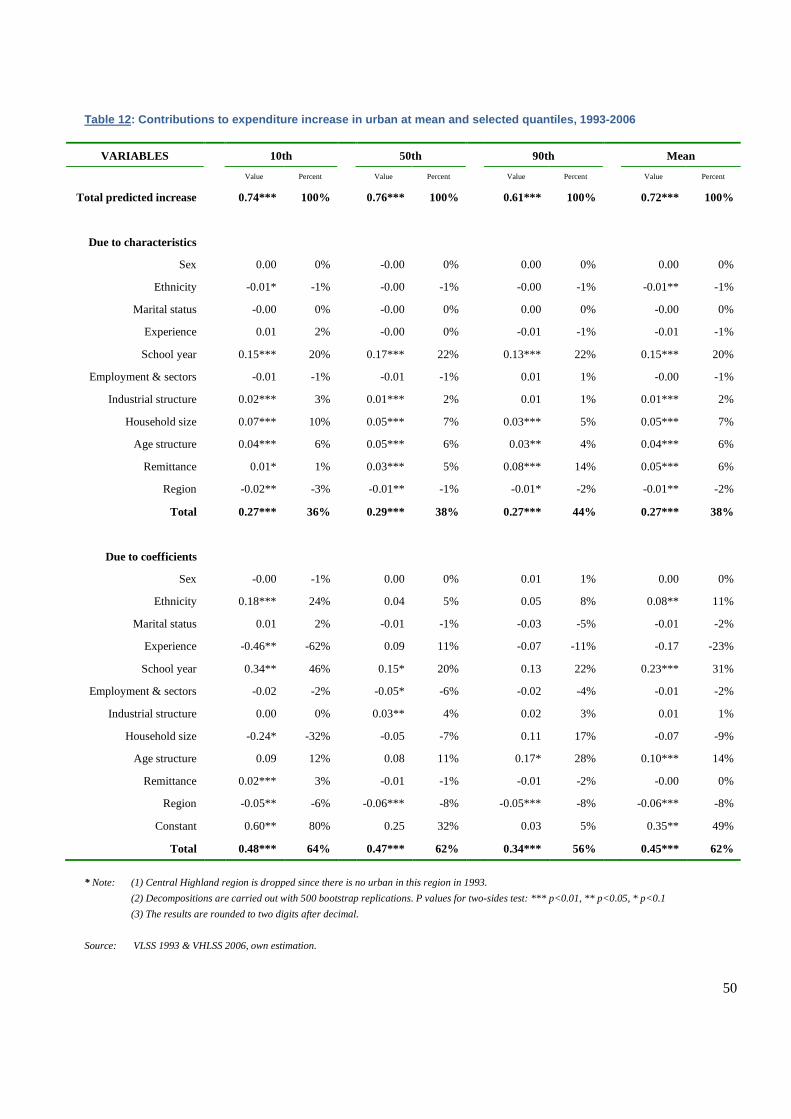
50

Table 12: Contributions to expenditure increase in urban at mean and selected quantiles, 1993-2006

VARIABLES 10th 50th 90th Mean

Value Percent Value Percent Value Percent Value Percent

Total predicted increase 0.74*** 100% 0.76*** 100% 0.61*** 100% 0.72*** 100%

Due to characteristics

Sex 0.00 0% -0.00 0% 0.00 0% 0.00 0%

Ethnicity -0.01* -1% -0.00 -1% -0.00 -1% -0.01** -1%

Marital status -0.00 0% -0.00 0% 0.00 0% -0.00 0%

Experience 0.01 2% -0.00 0% -0.01 -1% -0.01 -1%

School year 0.15*** 20% 0.17*** 22% 0.13*** 22% 0.15*** 20%

Employment & sectors -0.01 -1% -0.01 -1% 0.01 1% -0.00 -1%

Industrial structure 0.02*** 3% 0.01*** 2% 0.01 1% 0.01*** 2%

Household size 0.07*** 10% 0.05*** 7% 0.03*** 5% 0.05*** 7%

Age structure 0.04*** 6% 0.05*** 6% 0.03** 4% 0.04*** 6%

Remittance 0.01* 1% 0.03*** 5% 0.08*** 14% 0.05*** 6%

Region -0.02** -3% -0.01** -1% -0.01* -2% -0.01** -2%

Total 0.27*** 36% 0.29*** 38% 0.27*** 44% 0.27*** 38%

Due to coefficients

Sex -0.00 -1% 0.00 0% 0.01 1% 0.00 0%

Ethnicity 0.18*** 24% 0.04 5% 0.05 8% 0.08** 11%

Marital status 0.01 2% -0.01 -1% -0.03 -5% -0.01 -2%

Experience -0.46** -62% 0.09 11% -0.07 -11% -0.17 -23%

School year 0.34** 46% 0.15* 20% 0.13 22% 0.23*** 31%

Employment & sectors -0.02 -2% -0.05* -6% -0.02 -4% -0.01 -2%

Industrial structure 0.00 0% 0.03** 4% 0.02 3% 0.01 1%

Household size -0.24* -32% -0.05 -7% 0.11 17% -0.07 -9%

Age structure 0.09 12% 0.08 11% 0.17* 28% 0.10*** 14%

Remittance 0.02*** 3% -0.01 -1% -0.01 -2% -0.00 0%

Region -0.05** -6% -0.06*** -8% -0.05*** -8% -0.06*** -8%

Constant 0.60** 80% 0.25 32% 0.03 5% 0.35** 49%

Total 0.48*** 64% 0.47*** 62% 0.34*** 56% 0.45*** 62%

* Note: (1) Central Highland region is dropped since there is no urban in this region in 1993.

(2) Decompositions are carried out with 500 bootstrap replications. P values for two-sides test: *** p<0.01, ** p<0.05, * p<0.1

(3) The results are rounded to two digits after decimal.

Source: VLSS 1993 & VHLSS 2006, own estimation.

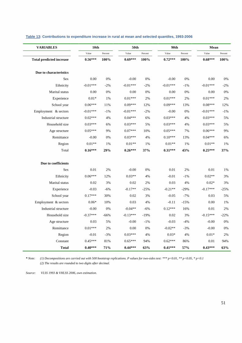
51

Table 13: Contributions to expenditure increase in rural at mean and selected quantiles, 1993-2006

VARIABLES 10th 50th 90th Mean

Value Percent Value Percent Value Percent Value Percent

Total predicted increase 0.56*** 100% 0.69*** 100% 0.72*** 100% 0.68*** 100%

Due to characteristics

Sex 0.00 0% -0.00 0% -0.00 0% 0.00 0%

Ethnicity -0.01*** -2% -0.01*** -2% -0.01*** -1% -0.01*** -2%

Marital status 0.00 0% 0.00 0% 0.00 0% 0.00 0%

Experience 0.01* 1% 0.01*** 2% 0.01*** 2% 0.01*** 2%

School year 0.06*** 11% 0.09*** 12% 0.09*** 13% 0.08*** 12%

Employment & sectors -0.01*** -1% -0.01*** -2% -0.00 0% -0.01*** -1%

Industrial structure 0.02*** 4% 0.04*** 6% 0.03*** 4% 0.03*** 5%

Household size 0.03*** 6% 0.03*** 5% 0.03*** 4% 0.03*** 5%

Age structure 0.05*** 9% 0.07*** 10% 0.05*** 7% 0.06*** 9%

Remittance -0.00 0% 0.03*** 4% 0.10*** 13% 0.04*** 6%

Region 0.01** 1% 0.01** 1% 0.01** 1% 0.01** 1%

Total 0.16*** 29% 0.26*** 37% 0.31*** 43% 0.25*** 37%

Due to coefficients

Sex 0.01 2% -0.00 0% 0.01 2% 0.01 1%

Ethnicity 0.06*** 12% 0.03** 4% -0.01 -1% 0.02** 3%

Marital status 0.02 3% 0.02 2% 0.03 4% 0.02* 3%

Experience -0.03 -6% -0.17** -25% -0.21** -29% -0.17*** -25%

School year 0.17*** 30% 0.02 3% -0.05 -7% 0.03 5%

Employment & sectors 0.06* 10% 0.03 4% -0.11 -15% 0.00 1%

Industrial structure -0.00 0% -0.04** -6% 0.12*** 16% 0.01 2%

Household size -0.37*** -66% -0.13*** -19% 0.02 3% -0.15*** -22%

Age structure 0.03 5% -0.00 -1% -0.03 -4% -0.00 0%

Remittance 0.01*** 2% 0.00 0% -0.02** -3% -0.00 0%

Region -0.01 -3% 0.03*** 4% 0.03* 4% 0.01* 2%

Constant 0.45*** 81% 0.65*** 94% 0.62*** 86% 0.01 94%

Total 0.40*** 71% 0.44*** 63% 0.41*** 57% 0.43*** 63%

* Note: (1) Decompositions are carried out with 500 bootstrap replications. P values for two-sides test: *** p<0.01, ** p<0.05, * p<0.1

(2) The results are rounded to two digits after decimal.

Source: VLSS 1993 & VHLSS 2006, own estimation.

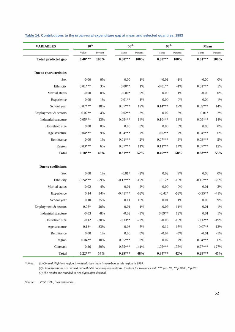
52

Table 14: Contributions to the urban-rural expenditure gap at mean and selected quantiles, 1993

VARIABLES 10th 50th 90th Mean

Value Percent Value Percent Value Percent Value Percent

Total predicted gap 0.40*** 100% 0.60*** 100% 0.80*** 100% 0.61*** 100%

Due to characteristics

Sex -0.00 0% 0.00 1% -0.01 -1% -0.00 0%

Ethnicity 0.01*** 3% 0.00** 1% -0.01** -1% 0.01*** 1%

Marital status -0.00 0% -0.00* 0% 0.00 1% -0.00 0%

Experience 0.00 1% 0.01** 1% 0.00 0% 0.00 1%

School year 0.07*** 18% 0.07*** 12% 0.14*** 17% 0.09*** 14%

Employment & sectors -0.02** -4% 0.02** 3% 0.02 3% 0.01* 2%

Industrial structure 0.05*** 13% 0.09*** 14% 0.10*** 13% 0.09*** 14%

Household size 0.00 0% 0.00 0% 0.00 0% 0.00 0%

Age structure 0.04*** 9% 0.04*** 7% 0.02** 2% 0.04*** 6%

Remittance 0.00 1% 0.01*** 2% 0.07*** 9% 0.03*** 5%

Region 0.03*** 6% 0.07*** 11% 0.11*** 14% 0.07*** 12%

Total 0.18*** 46% 0.31*** 52% 0.46*** 58% 0.33*** 55%

Due to coefficients

Sex 0.00 1% -0.01* -2% 0.02 3% 0.00 0%

Ethnicity -0.24*** -59% -0.12*** -19% -0.12* -15% -0.15*** -25%

Marital status 0.02 4% 0.01 2% -0.00 0% 0.01 2%

Experience 0.14 34% -0.41*** -68% -0.42* -53% -0.25** -41%

School year 0.10 25% 0.11 18% 0.01 1% 0.05 9%

Employment & sectors 0.08* 20% 0.01 1% -0.09 -11% -0.01 -1%

Industrial structure -0.03 -8% -0.02 -3% 0.09** 12% 0.01 1%

Household size -0.12 -30% -0.13** -22% -0.08 -10% -0.12** -19%

Age structure -0.13* -33% -0.03 -5% -0.12 -15% -0.07** -12%

Remittance 0.00 1% 0.00 0% -0.04 -5% -0.01 -1%

Region 0.04** 10% 0.05*** 8% 0.02 2% 0.04*** 6%

Constant 0.36 89% 0.85*** 141% 1.06*** 133% 0.77*** 127%

Total 0.22*** 54% 0.29*** 48% 0.34*** 42% 0.28*** 45%

* Note: (1) Central Highland region is omitted since there is no urban in this region in 1993.

(2) Decompositions are carried out with 500 bootstrap replications. P values for two-sides test: *** p<0.01, ** p<0.05, * p<0.1

(3) The results are rounded to two digits after decimal.

Source: VLSS 1993, own estimation.

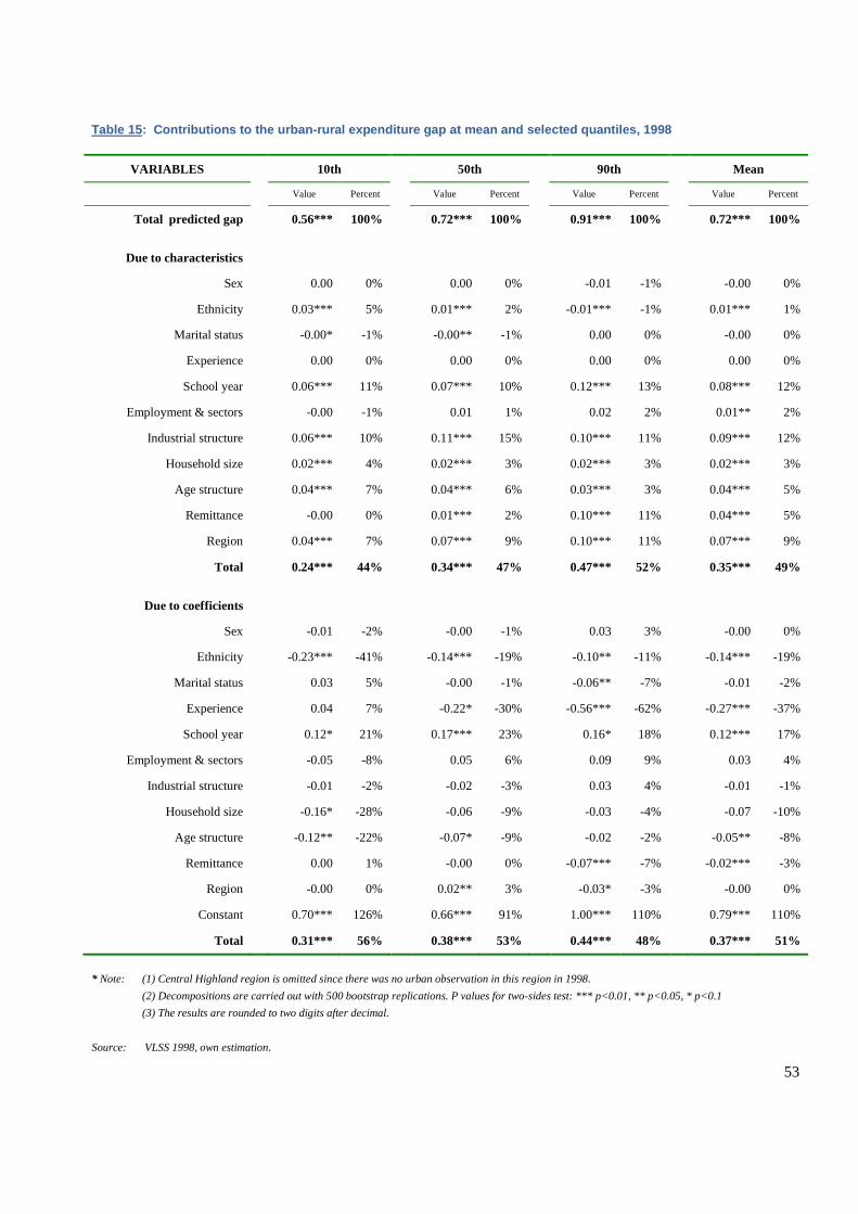
53

Table 15: Contributions to the urban-rural expenditure gap at mean and selected quantiles, 1998

VARIABLES 10th 50th 90th Mean

Value Percent Value Percent Value Percent Value Percent

Total predicted gap 0.56*** 100% 0.72*** 100% 0.91*** 100% 0.72*** 100%

Due to characteristics

Sex 0.00 0% 0.00 0% -0.01 -1% -0.00 0%

Ethnicity 0.03*** 5% 0.01*** 2% -0.01*** -1% 0.01*** 1%

Marital status -0.00* -1% -0.00** -1% 0.00 0% -0.00 0%

Experience 0.00 0% 0.00 0% 0.00 0% 0.00 0%

School year 0.06*** 11% 0.07*** 10% 0.12*** 13% 0.08*** 12%

Employment & sectors -0.00 -1% 0.01 1% 0.02 2% 0.01** 2%

Industrial structure 0.06*** 10% 0.11*** 15% 0.10*** 11% 0.09*** 12%

Household size 0.02*** 4% 0.02*** 3% 0.02*** 3% 0.02*** 3%

Age structure 0.04*** 7% 0.04*** 6% 0.03*** 3% 0.04*** 5%

Remittance -0.00 0% 0.01*** 2% 0.10*** 11% 0.04*** 5%

Region 0.04*** 7% 0.07*** 9% 0.10*** 11% 0.07*** 9%

Total 0.24*** 44% 0.34*** 47% 0.47*** 52% 0.35*** 49%

Due to coefficients

Sex -0.01 -2% -0.00 -1% 0.03 3% -0.00 0%

Ethnicity -0.23*** -41% -0.14*** -19% -0.10** -11% -0.14*** -19%

Marital status 0.03 5% -0.00 -1% -0.06** -7% -0.01 -2%

Experience 0.04 7% -0.22* -30% -0.56*** -62% -0.27*** -37%

School year 0.12* 21% 0.17*** 23% 0.16* 18% 0.12*** 17%

Employment & sectors -0.05 -8% 0.05 6% 0.09 9% 0.03 4%

Industrial structure -0.01 -2% -0.02 -3% 0.03 4% -0.01 -1%

Household size -0.16* -28% -0.06 -9% -0.03 -4% -0.07 -10%

Age structure -0.12** -22% -0.07* -9% -0.02 -2% -0.05** -8%

Remittance 0.00 1% -0.00 0% -0.07*** -7% -0.02*** -3%

Region -0.00 0% 0.02** 3% -0.03* -3% -0.00 0%

Constant 0.70*** 126% 0.66*** 91% 1.00*** 110% 0.79*** 110%

Total 0.31*** 56% 0.38*** 53% 0.44*** 48% 0.37*** 51%

* Note: (1) Central Highland region is omitted since there was no urban observation in this region in 1998.

(2) Decompositions are carried out with 500 bootstrap replications. P values for two-sides test: *** p<0.01, ** p<0.05, * p<0.1

(3) The results are rounded to two digits after decimal.

Source: VLSS 1998, own estimation.

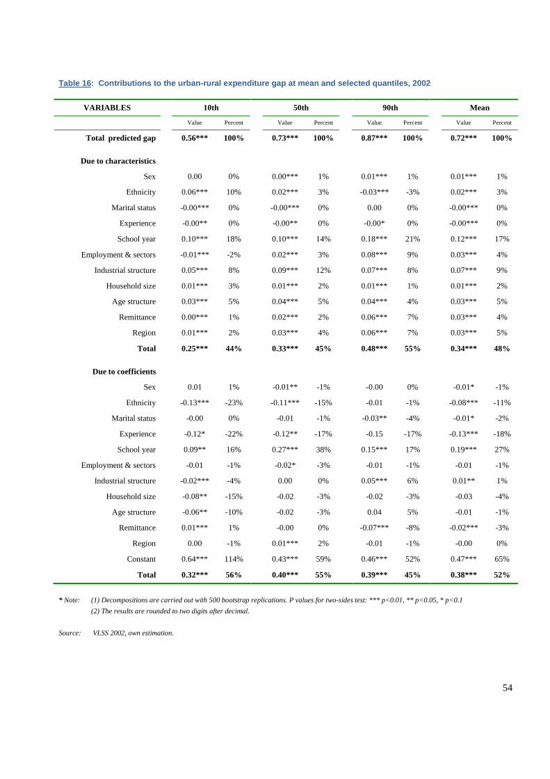
54

Table 16: Contributions to the urban-rural expenditure gap at mean and selected quantiles, 2002

VARIABLES 10th 50th 90th Mean

Value Percent Value Percent Value Percent Value Percent

Total predicted gap 0.56*** 100% 0.73*** 100% 0.87*** 100% 0.72*** 100%

Due to characteristics

Sex 0.00 0% 0.00*** 1% 0.01*** 1% 0.01*** 1%

Ethnicity 0.06*** 10% 0.02*** 3% -0.03*** -3% 0.02*** 3%

Marital status -0.00*** 0% -0.00*** 0% 0.00 0% -0.00*** 0%

Experience -0.00** 0% -0.00** 0% -0.00* 0% -0.00*** 0%

School year 0.10*** 18% 0.10*** 14% 0.18*** 21% 0.12*** 17%

Employment & sectors -0.01*** -2% 0.02*** 3% 0.08*** 9% 0.03*** 4%

Industrial structure 0.05*** 8% 0.09*** 12% 0.07*** 8% 0.07*** 9%

Household size 0.01*** 3% 0.01*** 2% 0.01*** 1% 0.01*** 2%

Age structure 0.03*** 5% 0.04*** 5% 0.04*** 4% 0.03*** 5%

Remittance 0.00*** 1% 0.02*** 2% 0.06*** 7% 0.03*** 4%

Region 0.01*** 2% 0.03*** 4% 0.06*** 7% 0.03*** 5%

Total 0.25*** 44% 0.33*** 45% 0.48*** 55% 0.34*** 48%

Due to coefficients

Sex 0.01 1% -0.01** -1% -0.00 0% -0.01* -1%

Ethnicity -0.13*** -23% -0.11*** -15% -0.01 -1% -0.08*** -11%

Marital status -0.00 0% -0.01 -1% -0.03** -4% -0.01* -2%

Experience -0.12* -22% -0.12** -17% -0.15 -17% -0.13*** -18%

School year 0.09** 16% 0.27*** 38% 0.15*** 17% 0.19*** 27%

Employment & sectors -0.01 -1% -0.02* -3% -0.01 -1% -0.01 -1%

Industrial structure -0.02*** -4% 0.00 0% 0.05*** 6% 0.01** 1%

Household size -0.08** -15% -0.02 -3% -0.02 -3% -0.03 -4%

Age structure -0.06** -10% -0.02 -3% 0.04 5% -0.01 -1%

Remittance 0.01*** 1% -0.00 0% -0.07*** -8% -0.02*** -3%

Region 0.00 -1% 0.01*** 2% -0.01 -1% -0.00 0%

Constant 0.64*** 114% 0.43*** 59% 0.46*** 52% 0.47*** 65%

Total 0.32*** 56% 0.40*** 55% 0.39*** 45% 0.38*** 52%

* Note: (1) Decompositions are carried out with 500 bootstrap replications. P values for two-sides test: *** p<0.01, ** p<0.05, * p<0.1

(2) The results are rounded to two digits after decimal.

Source: VLSS 2002, own estimation.

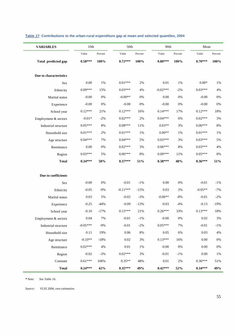
55

Table 17: Contributions to the urban-rural expenditure gap at mean and selected quantiles, 2004

VARIABLES 10th 50th 90th Mean

Value Percent Value Percent Value Percent Value Percent

Total predicted gap 0.58*** 100% 0.72*** 100% 0.80*** 100% 0.70*** 100%

Due to characteristics

Sex 0.00 1% 0.01*** 2% 0.01 1% 0.00* 1%

Ethnicity 0.09*** 15% 0.03*** 4% -0.02*** -2% 0.03*** 4%

Marital status -0.00 0% -0.00** 0% 0.00 0% -0.00 0%

Experience -0.00 0% -0.00 0% -0.00 0% -0.00 0%

School year 0.12*** 21% 0.12*** 16% 0.14*** 17% 0.12*** 18%

Employment & sectors -0.01* -2% 0.02*** 2% 0.04*** 6% 0.02*** 3%

Industrial structure 0.05*** 8% 0.08*** 11% 0.03** 3% 0.06*** 8%

Household size 0.01*** 2% 0.01*** 1% 0.00** 1% 0.01*** 1%

Age structure 0.04*** 7% 0.04*** 5% 0.03*** 3% 0.03*** 5%

Remittance 0.00 0% 0.02*** 3% 0.06*** 8% 0.03*** 4%

Region 0.03*** 5% 0.06*** 8% 0.09*** 11% 0.05*** 8%

Total 0.34*** 58% 0.37*** 51% 0.38*** 48% 0.36*** 51%

Due to coefficients

Sex -0.00 0% -0.01 -1% 0.00 0% -0.01 -1%

Ethnicity -0.05 -9% -0.11*** -15% 0.03 3% -0.05** -7%

Marital status 0.03 5% -0.02 -3% -0.06** -8% -0.01 -2%

Experience -0.25 -44% -0.09 -13% -0.03 -4% -0.13 -19%

School year -0.10 -17% 0.15*** 21% 0.26*** 33% 0.13*** 18%

Employment & sectors 0.04 7% -0.01 -1% -0.00 0% 0.02 3%

Industrial structure -0.05*** -9% -0.01 -2% 0.05*** 7% -0.01 -1%

Household size 0.11 19% 0.06 8% 0.05 6% 0.03 4%

Age structure -0.10** -18% 0.02 3% 0.13*** 16% 0.00 0%

Remittance 0.02*** 4% 0.01 1% -0.00 0% 0.00 0%

Region -0.02 -3% 0.02*** 3% -0.01 -1% 0.00 1%

Constant 0.61*** 106% 0.35** 48% 0.01 2% 0.36*** 51%

Total 0.24*** 42% 0.35*** 49% 0.42*** 52% 0.34*** 49%

* Note: See Table 16.

Source: VLSS 2004, own estimation.

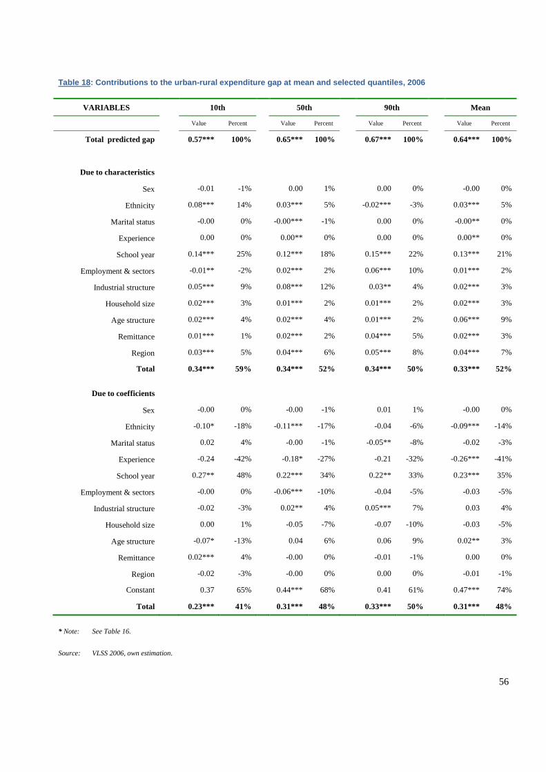
56

Table 18: Contributions to the urban-rural expenditure gap at mean and selected quantiles, 2006

VARIABLES 10th 50th 90th Mean

Value Percent Value Percent Value Percent Value Percent

Total predicted gap 0.57*** 100% 0.65*** 100% 0.67*** 100% 0.64*** 100%

Due to characteristics

Sex -0.01 -1% 0.00 1% 0.00 0% -0.00 0%

Ethnicity 0.08*** 14% 0.03*** 5% -0.02*** -3% 0.03*** 5%

Marital status -0.00 0% -0.00*** -1% 0.00 0% -0.00** 0%

Experience 0.00 0% 0.00** 0% 0.00 0% 0.00** 0%

School year 0.14*** 25% 0.12*** 18% 0.15*** 22% 0.13*** 21%

Employment & sectors -0.01** -2% 0.02*** 2% 0.06*** 10% 0.01*** 2%

Industrial structure 0.05*** 9% 0.08*** 12% 0.03** 4% 0.02*** 3%

Household size 0.02*** 3% 0.01*** 2% 0.01*** 2% 0.02*** 3%

Age structure 0.02*** 4% 0.02*** 4% 0.01*** 2% 0.06*** 9%

Remittance 0.01*** 1% 0.02*** 2% 0.04*** 5% 0.02*** 3%

Region 0.03*** 5% 0.04*** 6% 0.05*** 8% 0.04*** 7%

Total 0.34*** 59% 0.34*** 52% 0.34*** 50% 0.33*** 52%

Due to coefficients

Sex -0.00 0% -0.00 -1% 0.01 1% -0.00 0%

Ethnicity -0.10* -18% -0.11*** -17% -0.04 -6% -0.09*** -14%

Marital status 0.02 4% -0.00 -1% -0.05** -8% -0.02 -3%

Experience -0.24 -42% -0.18* -27% -0.21 -32% -0.26*** -41%

School year 0.27** 48% 0.22*** 34% 0.22** 33% 0.23*** 35%

Employment & sectors -0.00 0% -0.06*** -10% -0.04 -5% -0.03 -5%

Industrial structure -0.02 -3% 0.02** 4% 0.05*** 7% 0.03 4%

Household size 0.00 1% -0.05 -7% -0.07 -10% -0.03 -5%

Age structure -0.07* -13% 0.04 6% 0.06 9% 0.02** 3%

Remittance 0.02*** 4% -0.00 0% -0.01 -1% 0.00 0%

Region -0.02 -3% -0.00 0% 0.00 0% -0.01 -1%

Constant 0.37 65% 0.44*** 68% 0.41 61% 0.47*** 74%

Total 0.23*** 41% 0.31*** 48% 0.33*** 50% 0.31*** 48%

* Note: See Table 16.

Source: VLSS 2006, own estimation.

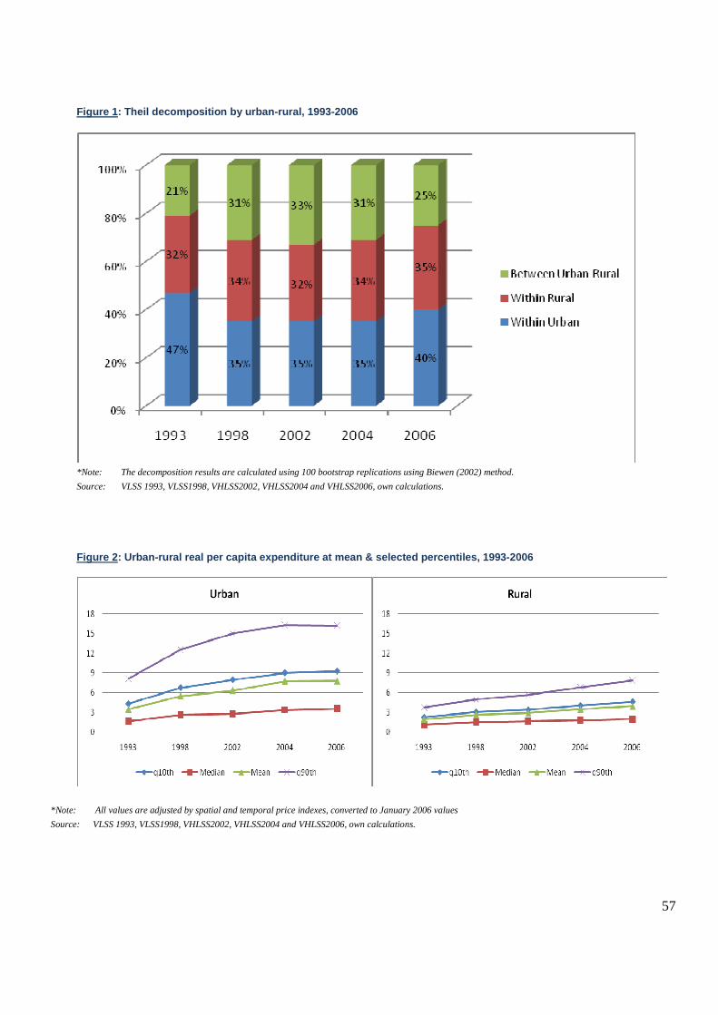
57

Figure 1: Theil decomposition by urban-rural, 1993-2006

*Note: The decomposition results are calculated using 100 bootstrap replications using Biewen (2002) method.

Source: VLSS 1993, VLSS1998, VHLSS2002, VHLSS2004 and VHLSS2006, own calculations.

Figure 2: Urban-rural real per capita expenditure at mean & selected percentiles, 1993-2006

*Note: All values are adjusted by spatial and temporal price indexes, converted to January 2006 values

Source: VLSS 1993, VLSS1998, VHLSS2002, VHLSS2004 and VHLSS2006, own calculations.

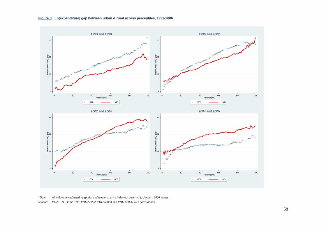
58

Figure 3: Ln(expenditure) gap between urban & rural across percentiles, 1993-2006

.4.6

.81

Ln(e

xpen

ditu

re)

gap

0 20 40 60 80 100Percentiles

1998 1993

1993 and 1998

.4.6

.81

Ln(e

xpen

ditu

re)

gap

0 20 40 60 80 100Percentiles

2002 1998

1998 and 2002

.4.6

.81

Ln(e

xpen

ditu

re)

gap

0 20 40 60 80 100Percentiles

2004 2002

2002 and 2004

.4.6

.81

Ln(e

xpen

ditu

re)

gap

0 20 40 60 80 100Percentiles

2006 2004

2004 and 2006

*Note: All values are adjusted by spatial and temporal price indexes, converted to January 2006 values

Source: VLSS 1993, VLSS1998, VHLSS2002, VHLSS2004 and VHLSS2006, own calculations.

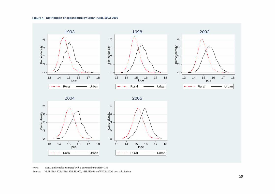
59

Figure 4: Distribution of expenditure by urban-rural, 1993-2006

0.2

.4.6

.8K

erne

l den

sity

13 14 15 16 17 18lpce

Rural Urban

1993

0.2

.4.6

.8K

erne

l den

sity

13 14 15 16 17 18lpce

Rural Urban

1998

0.2

.4.6

.8K

erne

l den

sity

13 14 15 16 17 18lpce

Rural Urban

2002

0.2

.4.6

.8K

erne

l den

sity

13 14 15 16 17 18lpce

Rural Urban

2004

0.2

.4.6

.8K

erne

l den

sity

13 14 15 16 17 18lpce

Rural Urban

2006

*Note: Gaussian kernel is estimated with a common bandwidth=0.08

Source: VLSS 1993, VLSS1998, VHLSS2002, VHLSS2004 and VHLSS2006, own calculations

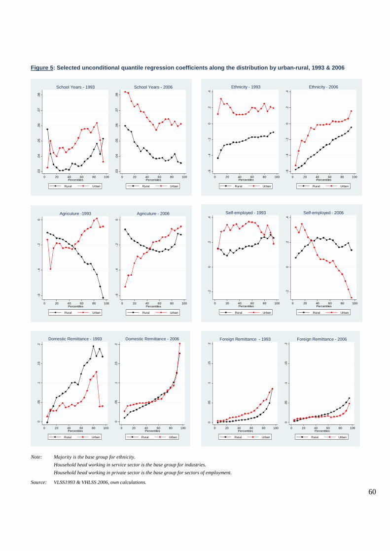
60

Figure 5: Selected unconditional quantile regression coefficients along the distribution by urban-rural, 1993 & 2006

.03

.04

.05

.06

.07

.08

0 20 40 60 80 100Percentiles

Rural Urban

School Years - 1993

.03

.04

.05

.06

.07

.08

0 20 40 60 80 100Percentiles

Rural Urban

School Years - 2006

-.6

-.4

-.2

0.2

.4

0 20 40 60 80 100Percentiles

Rural Urban

Ethnicity - 1993

-.6

-.4

-.2

0.2

.4

0 20 40 60 80 100Percentiles

Rural Urban

Ethnicity - 2006

-.6

-.4

-.2

0

0 20 40 60 80 100Percentiles

Rural Urban

Agricuture -1993

-.6

-.4

-.2

0

0 20 40 60 80 100Percentiles

Rural Urban

Agricuture - 2006

-.2

0.2

.4

0 20 40 60 80 100Percentiles

Rural Urban

Self-employed - 1993

-.2

0.2

.4

0 20 40 60 80 100Percentiles

Rural Urban

Self-employed - 2006

0.0

5.1

.15

.2

0 20 40 60 80 100Percentiles

Rural Urban

Domestic Remittance - 1993

0.0

5.1

.15

.2

0 20 40 60 80 100Percentiles

Rural Urban

Domestic Remittance - 2006

0.0

5.1

.15

.2

0 20 40 60 80 100Percentiles

Rural Urban

Foreign Remittance - 1993

0.0

5.1

.15

.2

0 20 40 60 80 100Percentiles

Rural Urban

Foreign Remittance - 2006

Note: Majority is the base group for ethnicity.

Household head working in service sector is the base group for industries.

Household head working in private sector is the base group for sectors of employment.

Source: VLSS1993 & VHLSS 2006, own calculations.

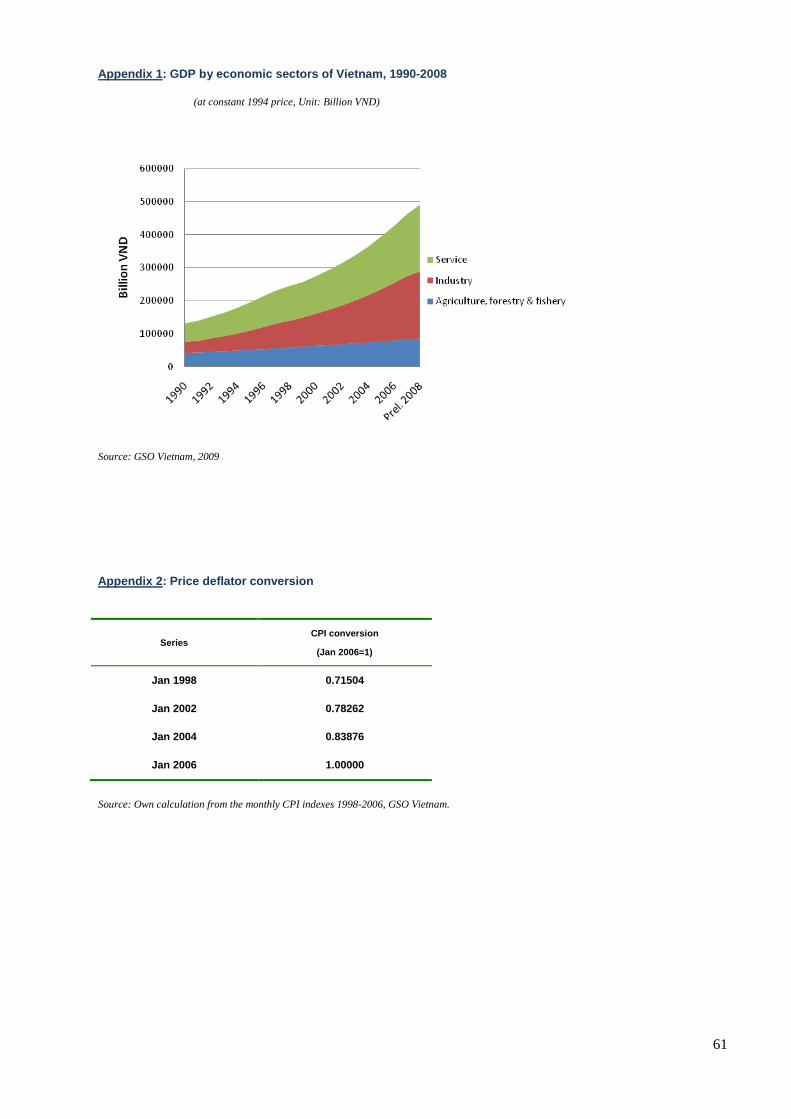
61

Appendix 1: GDP by economic sectors of Vietnam, 1990-2008

(at constant 1994 price, Unit: Billion VND)

Source: GSO Vietnam, 2009

Appendix 2: Price deflator conversion

Series CPI conversion

(Jan 2006=1)

Jan 1998 0.71504

Jan 2002 0.78262

Jan 2004 0.83876

Jan 2006 1.00000

Source: Own calculation from the monthly CPI indexes 1998-2006, GSO Vietnam.

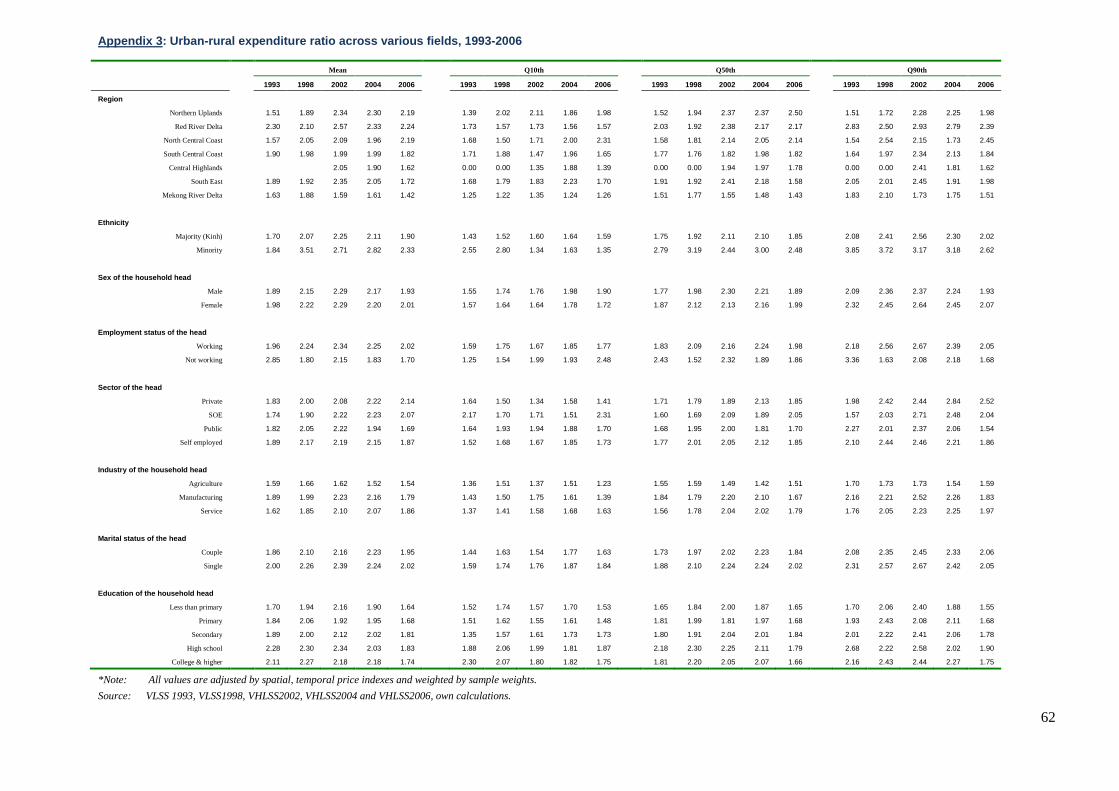
62

Appendix 3: Urban-rural expenditure ratio across various fields, 1993-2006

Mean Q10th Q50th Q90th

1993 1998 2002 2004 2006 1993 1998 2002 2004 2006 1993 1998 2002 2004 2006 1993 1998 2002 2004 2006

Region

Northern Uplands 1.51 1.89 2.34 2.30 2.19 1.39 2.02 2.11 1.86 1.98 1.52 1.94 2.37 2.37 2.50 1.51 1.72 2.28 2.25 1.98

Red River Delta 2.30 2.10 2.57 2.33 2.24 1.73 1.57 1.73 1.56 1.57 2.03 1.92 2.38 2.17 2.17 2.83 2.50 2.93 2.79 2.39

North Central Coast 1.57 2.05 2.09 1.96 2.19 1.68 1.50 1.71 2.00 2.31 1.58 1.81 2.14 2.05 2.14 1.54 2.54 2.15 1.73 2.45

South Central Coast 1.90 1.98 1.99 1.99 1.82 1.71 1.88 1.47 1.96 1.65 1.77 1.76 1.82 1.98 1.82 1.64 1.97 2.34 2.13 1.84

Central Highlands 2.05 1.90 1.62 0.00 0.00 1.35 1.88 1.39 0.00 0.00 1.94 1.97 1.78 0.00 0.00 2.41 1.81 1.62

South East 1.89 1.92 2.35 2.05 1.72 1.68 1.79 1.83 2.23 1.70 1.91 1.92 2.41 2.18 1.58 2.05 2.01 2.45 1.91 1.98

Mekong River Delta 1.63 1.88 1.59 1.61 1.42 1.25 1.22 1.35 1.24 1.26 1.51 1.77 1.55 1.48 1.43 1.83 2.10 1.73 1.75 1.51

Ethnicity

Majority (Kinh) 1.70 2.07 2.25 2.11 1.90 1.43 1.52 1.60 1.64 1.59 1.75 1.92 2.11 2.10 1.85 2.08 2.41 2.56 2.30 2.02

Minority 1.84 3.51 2.71 2.82 2.33 2.55 2.80 1.34 1.63 1.35 2.79 3.19 2.44 3.00 2.48 3.85 3.72 3.17 3.18 2.62

Sex of the household head

Male 1.89 2.15 2.29 2.17 1.93 1.55 1.74 1.76 1.98 1.90 1.77 1.98 2.30 2.21 1.89 2.09 2.36 2.37 2.24 1.93

Female 1.98 2.22 2.29 2.20 2.01 1.57 1.64 1.64 1.78 1.72 1.87 2.12 2.13 2.16 1.99 2.32 2.45 2.64 2.45 2.07

Employment status of the head

Working 1.96 2.24 2.34 2.25 2.02 1.59 1.75 1.67 1.85 1.77 1.83 2.09 2.16 2.24 1.98 2.18 2.56 2.67 2.39 2.05

Not working 2.85 1.80 2.15 1.83 1.70 1.25 1.54 1.99 1.93 2.48 2.43 1.52 2.32 1.89 1.86 3.36 1.63 2.08 2.18 1.68

Sector of the head

Private 1.83 2.00 2.08 2.22 2.14 1.64 1.50 1.34 1.58 1.41 1.71 1.79 1.89 2.13 1.85 1.98 2.42 2.44 2.84 2.52

SOE 1.74 1.90 2.22 2.23 2.07 2.17 1.70 1.71 1.51 2.31 1.60 1.69 2.09 1.89 2.05 1.57 2.03 2.71 2.48 2.04

Public 1.82 2.05 2.22 1.94 1.69 1.64 1.93 1.94 1.88 1.70 1.68 1.95 2.00 1.81 1.70 2.27 2.01 2.37 2.06 1.54

Self employed 1.89 2.17 2.19 2.15 1.87 1.52 1.68 1.67 1.85 1.73 1.77 2.01 2.05 2.12 1.85 2.10 2.44 2.46 2.21 1.86

Industry of the household head

Agriculture 1.59 1.66 1.62 1.52 1.54 1.36 1.51 1.37 1.51 1.23 1.55 1.59 1.49 1.42 1.51 1.70 1.73 1.73 1.54 1.59

Manufacturing 1.89 1.99 2.23 2.16 1.79 1.43 1.50 1.75 1.61 1.39 1.84 1.79 2.20 2.10 1.67 2.16 2.21 2.52 2.26 1.83

Service 1.62 1.85 2.10 2.07 1.86 1.37 1.41 1.58 1.68 1.63 1.56 1.78 2.04 2.02 1.79 1.76 2.05 2.23 2.25 1.97

Marital status of the head

Couple 1.86 2.10 2.16 2.23 1.95 1.44 1.63 1.54 1.77 1.63 1.73 1.97 2.02 2.23 1.84 2.08 2.35 2.45 2.33 2.06

Single 2.00 2.26 2.39 2.24 2.02 1.59 1.74 1.76 1.87 1.84 1.88 2.10 2.24 2.24 2.02 2.31 2.57 2.67 2.42 2.05

Education of the household head

Less than primary 1.70 1.94 2.16 1.90 1.64 1.52 1.74 1.57 1.70 1.53 1.65 1.84 2.00 1.87 1.65 1.70 2.06 2.40 1.88 1.55

Primary 1.84 2.06 1.92 1.95 1.68 1.51 1.62 1.55 1.61 1.48 1.81 1.99 1.81 1.97 1.68 1.93 2.43 2.08 2.11 1.68

Secondary 1.89 2.00 2.12 2.02 1.81 1.35 1.57 1.61 1.73 1.73 1.80 1.91 2.04 2.01 1.84 2.01 2.22 2.41 2.06 1.78

High school 2.28 2.30 2.34 2.03 1.83 1.88 2.06 1.99 1.81 1.87 2.18 2.30 2.25 2.11 1.79 2.68 2.22 2.58 2.02 1.90

College & higher 2.11 2.27 2.18 2.18 1.74 2.30 2.07 1.80 1.82 1.75 1.81 2.20 2.05 2.07 1.66 2.16 2.43 2.44 2.27 1.75

*Note: All values are adjusted by spatial, temporal price indexes and weighted by sample weights.

Source: VLSS 1993, VLSS1998, VHLSS2002, VHLSS2004 and VHLSS2006, own calculations.

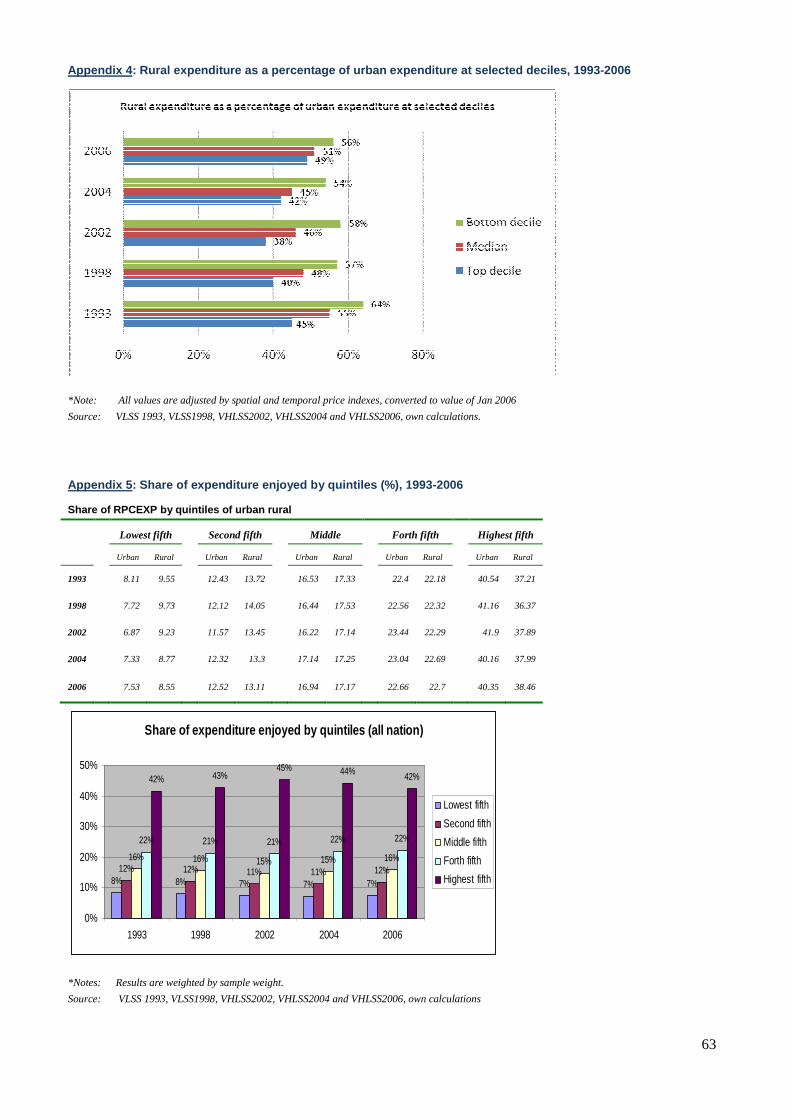
63

Appendix 4: Rural expenditure as a percentage of urban expenditure at selected deciles, 1993-2006

*Note: All values are adjusted by spatial and temporal price indexes, converted to value of Jan 2006

Source: VLSS 1993, VLSS1998, VHLSS2002, VHLSS2004 and VHLSS2006, own calculations.

Appendix 5: Share of expenditure enjoyed by quintiles (%), 1993-2006

Share of RPCEXP by quintiles of urban rural

Lowest fifth Second fifth Middle Forth fifth Highest fifth

Urban Rural Urban Rural Urban Rural Urban Rural Urban Rural

1993 8.11 9.55 12.43 13.72 16.53 17.33 22.4 22.18 40.54 37.21

1998 7.72 9.73 12.12 14.05 16.44 17.53 22.56 22.32 41.16 36.37

2002 6.87 9.23 11.57 13.45 16.22 17.14 23.44 22.29 41.9 37.89

2004 7.33 8.77 12.32 13.3 17.14 17.25 23.04 22.69 40.16 37.99

2006 7.53 8.55 12.52 13.11 16.94 17.17 22.66 22.7 40.35 38.46

Share of expenditure enjoyed by quintiles (all nation)

8% 8% 7% 7% 7%

12% 12% 11% 11% 12%16% 16% 15% 15% 16%

22% 21% 21% 22% 22%

42% 43%45% 44% 42%

0%

10%

20%

30%

40%

50%

1993 1998 2002 2004 2006

Lowest fifth

Second fifth

Middle fifth

Forth fifth

Highest fifth

*Notes: Results are weighted by sample weight.

Source: VLSS 1993, VLSS1998, VHLSS2002, VHLSS2004 and VHLSS2006, own calculations

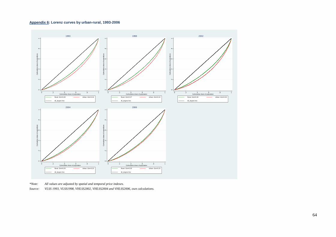
64

Appendix 6: Lorenz curves by urban-rural, 1993-2006

0.2

.4.6

.81

Cul

mu

lativ

e sh

are

of e

xpen

ditu

re

0 .2 .4 .6 .8 1Culmulative share of population

Rural: Gini=0.28 Urban: Gini=0.34

45_degree line

1993

0.2

.4.6

.81

Cul

mu

lativ

e sh

are

of e

xpen

ditu

re

0 .2 .4 .6 .8 1Culmulative share of population

Rural: Gini=0.27 Urban: Gini=0.34

45_degree line

1998

0.2

.4.6

.81

Cul

mu

lativ

e sh

are

of e

xpen

ditu

re

0 .2 .4 .6 .8 1Culmulative share of population

Rural: Gini=0.28 Urban: Gini=0.35

45_degree line

20020

.2.4

.6.8

1C

ulm

ulat

ive

shar

e of

exp

end

iture

0 .2 .4 .6 .8 1Culmulative share of population

Rural: Gini=0.29 Urban: Gini=0.33

45_degree line

20040

.2.4

.6.8

1C

ulm

ulat

ive

shar

e of

exp

end

iture

0 .2 .4 .6 .8 1Culmulative share of population

Rural: Gini=0.30 Urban: Gini=0.33

45_degree line

2006

*Note: All values are adjusted by spatial and temporal price indexes.

Source: VLSS 1993, VLSS1998, VHLSS2002, VHLSS2004 and VHLSS2006, own calculations.

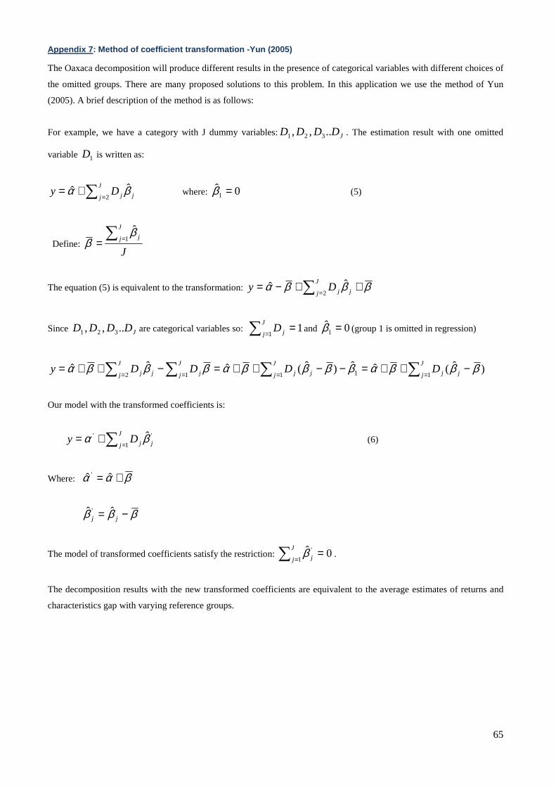
65

Appendix 7: Method of coefficient transformation -Yun (2005)

The Oaxaca decomposition will produce different results in the presence of categorical variables with different choices of

the omitted groups. There are many proposed solutions to this problem. In this application we use the method of Yun

(2005). A brief description of the method is as follows:

For example, we have a category with J dummy variables: JDDDD ..,, 321 . The estimation result with one omitted

variable 1D is written as:

j

J

j jDy βα ˆˆ2∑ =

+= where: 0ˆ1 =β (5)

Define: J

J

j j∑ == 1β

β

The equation (5) is equivalent to the transformation: βββα ++−= ∑ = j

J

j jDy ˆˆ2

Since JDDDD ..,, 321 are categorical variables so: 11

=∑ =

J

j jD and 0ˆ1 =β (group 1 is omitted in regression)

)ˆ(ˆˆ)ˆ(ˆˆˆ11112

βββαββββαβββα −++=−−++=−++= ∑∑∑∑ ==== j

J

j jj

J

j j

J

j jj

J

j j DDDDy

Our model with the transformed coefficients is:

∑ =+= J

j jjDy1

'' βα (6)

Where: βαα += ˆˆ '

βββ −= jjˆˆ '

The model of transformed coefficients satisfy the restriction: ∑ ==J

j j1

' 0β .

The decomposition results with the new transformed coefficients are equivalent to the average estimates of returns and

characteristics gap with varying reference groups.

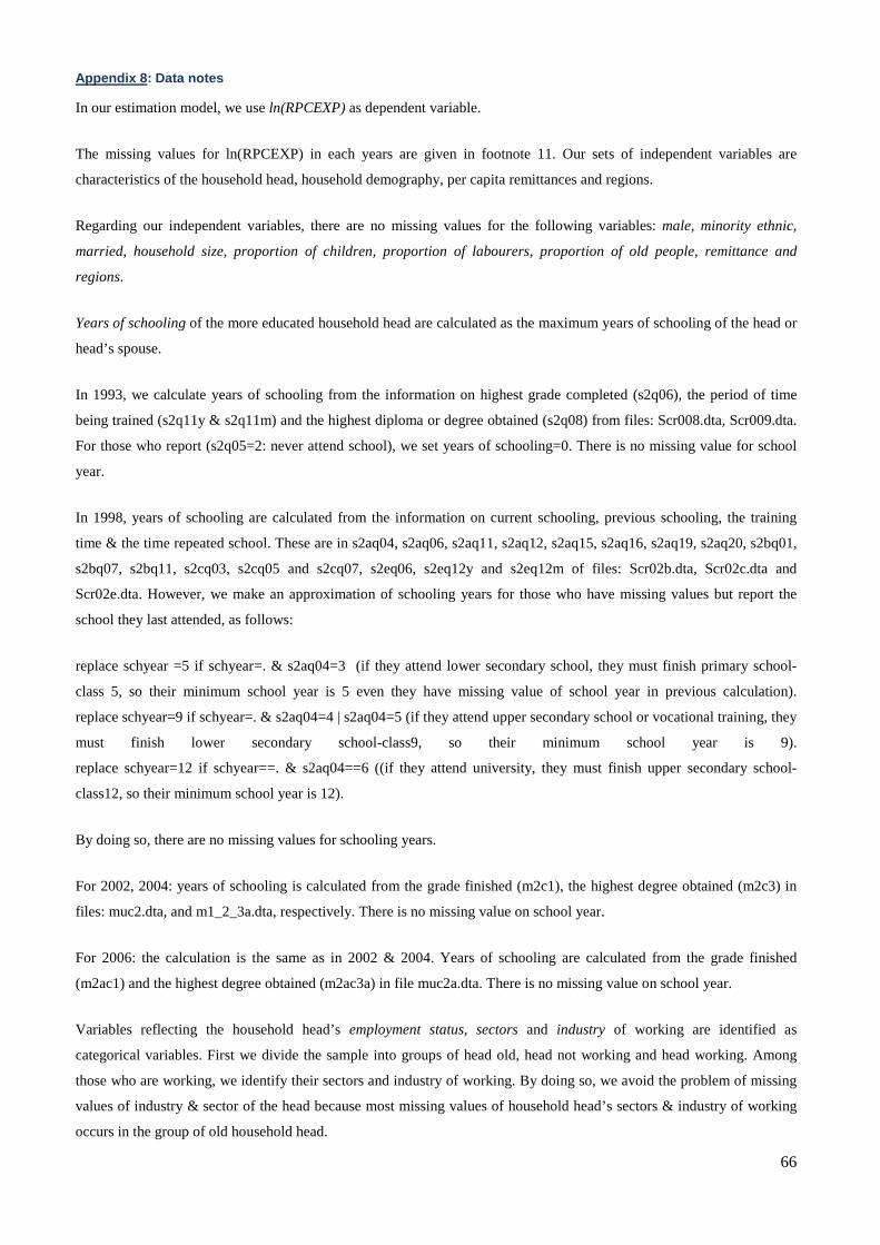
66

Appendix 8: Data notes

In our estimation model, we use ln(RPCEXP) as dependent variable.

The missing values for ln(RPCEXP) in each years are given in footnote 11. Our sets of independent variables are

characteristics of the household head, household demography, per capita remittances and regions.

Regarding our independent variables, there are no missing values for the following variables: male, minority ethnic,

married, household size, proportion of children, proportion of labourers, proportion of old people, remittance and

regions.

Years of schooling of the more educated household head are calculated as the maximum years of schooling of the head or

head’s spouse.

In 1993, we calculate years of schooling from the information on highest grade completed (s2q06), the period of time

being trained (s2q11y & s2q11m) and the highest diploma or degree obtained (s2q08) from files: Scr008.dta, Scr009.dta.

For those who report (s2q05=2: never attend school), we set years of schooling=0. There is no missing value for school

year.

In 1998, years of schooling are calculated from the information on current schooling, previous schooling, the training

time & the time repeated school. These are in s2aq04, s2aq06, s2aq11, s2aq12, s2aq15, s2aq16, s2aq19, s2aq20, s2bq01,

s2bq07, s2bq11, s2cq03, s2cq05 and s2cq07, s2eq06, s2eq12y and s2eq12m of files: Scr02b.dta, Scr02c.dta and

Scr02e.dta. However, we make an approximation of schooling years for those who have missing values but report the

school they last attended, as follows:

replace schyear =5 if schyear=. & s2aq04=3 (if they attend lower secondary school, they must finish primary school-

class 5, so their minimum school year is 5 even they have missing value of school year in previous calculation).

replace schyear=9 if schyear=. & s2aq04=4 | s2aq04=5 (if they attend upper secondary school or vocational training, they

must finish lower secondary school-class9, so their minimum school year is 9).

replace schyear=12 if schyear==. & s2aq04==6 ((if they attend university, they must finish upper secondary school-

class12, so their minimum school year is 12).

By doing so, there are no missing values for schooling years.

For 2002, 2004: years of schooling is calculated from the grade finished (m2c1), the highest degree obtained (m2c3) in

files: muc2.dta, and m1_2_3a.dta, respectively. There is no missing value on school year.

For 2006: the calculation is the same as in 2002 & 2004. Years of schooling are calculated from the grade finished

(m2ac1) and the highest degree obtained (m2ac3a) in file muc2a.dta. There is no missing value on school year.

Variables reflecting the household head’s employment status, sectors and industry of working are identified as

categorical variables. First we divide the sample into groups of head old, head not working and head working. Among

those who are working, we identify their sectors and industry of working. By doing so, we avoid the problem of missing

values of industry & sector of the head because most missing values of household head’s sectors & industry of working

occurs in the group of old household head.