Embed Size (px)
Citation preview

ISSN No. 2454 – 1427
CDE (Revised Version) April 2016
Decomposition Analysis of Earnings Inequality
in Rural India: 2004-2012
Shantanu Khanna Email: [email protected]
Department of Economics
Delhi School of Economics
Deepti Goel Email: [email protected]
Department of Economics
Delhi School of Economics
René Morissette Email: [email protected]
Statistics Canada
(Revised Version, April 2016)
Working Paper No. 250
http://www.cdedse.org/working-paper-frameset.htm
CENTRE FOR DEVELOPMENT ECONOMICS DELHI SCHOOL OF ECONOMICS
DELHI 110007

1
Decomposition Analysis of Earnings Inequality
in Rural India: 2004-2012
Shantanu Khanna
University of Delhi, [email protected]
Deepti Goel
Delhi School of Economics, [email protected]
René Morissette
Statistics Canada, [email protected]
April 2016
*The research leading to these results has received funding from the European Community’s Seventh Framework Programme (FP7/2007-2013) under grant agreement n° 290752. The views expressed in this paper are those of the authors and do not reflect the views of Statistics Canada, or of other institutions that the authors are affiliated to.

2
Abstract: We analyze the changes in earnings of paid workers (wage earners) in rural India from 2004/05
to 2011/12. Real earnings increased at all percentiles, and the percentage increase was larger at the lower
end. Consequently, earnings inequality declined. Recentered Influence Function decompositions show
that throughout the earnings distribution, except at the very top, both changes in ‘worker characteristics’
and in ‘returns to these characteristics’ increased earnings, with the latter having played a bigger role.
Decompositions of inequality measures reveal that although the change in characteristics had an
inequality increasing effect, chiefly attributable to increased education levels, inequality declined because
workers at lower quantiles experienced greater improvements in returns to their characteristics than
those at the top.
JEL Codes: J30, J31, O53
Keywords: Earnings, Inequality, Earnings Distribution, Rural India

3
1 Introduction
In their discussion of India’s economic growth, Kotwal et al (2011) point to the existence of two Indias:
“One of educated managers and engineers who have been able to take advantage of the opportunities
made available through globalization and the other—a huge mass of undereducated people who are
making a living in low productivity jobs in the informal sector—the largest of which is still agriculture.”
This paper is about the second India that mainly resides in its rural parts. Agriculture, the mainstay of the
rural economy, continues to employ the largest share of the Indian workforce, but its contribution to gross
value added is much smaller. In 2011, the employment shares of agriculture, industry, and services were
49, 24 and 27 percent respectively, whereas their shares in Gross Value Added were 19, 33, and 48 percent
respectively (GOI 2015). In addition, between 2004/05 and 2011/12, real Gross Domestic Product in these
sectors grew at 4.2, 8.5 and 9.6 percent per annum, respectively, making agriculture the slowest growing
sector of the economy (authors’ calculations based on RBI 2015). Given these figures, the concern about
whether high overall GDP growth has benefitted those at the bottom, and to what extent they have
benefitted compared to those at the top, is even more pertinent for rural India. We therefore focus on
rural India and examine how real earnings of paid workers (wage earners) evolved over the seven-year
period between 2004/05 and 2011/12.
Several studies have documented that along with the high growth rates of GDP that have characterized
the Indian economy since the 1980s, there has been an increase in inequality.1 However, most of these
studies have either focused on consumption expenditure (Sen and Himanshu 2004; Cain et al 2010;
Motiram and Vakulabharanam 2013; Jayaraj and Subramanian 2015; Datt et al 2016),2 or on earnings of
1 A notable exception is Dutta (2005). For the period, 1983-99, at the all-India level she finds an increase in wage rate inequality among regular salaried workers, but a decrease among casual labor. 2 There are some advantages in looking at consumption expenditure instead of earnings (Goldberg and Pavcnik 2007). The former are a better measure of lifetime wellbeing and suffer from fewer reporting errors. In spite of this, we feel that it is important to juxtapose the two to get a complete picture. This is especially important as the two

4
paid workers in urban India (Kijima 2006; Azam 2012). Two notable exceptions are Hnatkovska and Lahiri
2013, and Jacoby and Dasgupta 2015. Hnatkovska and Lahiri (2013) focus on wage comparisons between
rural and urban areas between 1983 and 2010. They find that urban agglomeration led to a massive
increase in urban labor supply that in turn reduced the rural-urban wage gap. Unlike Hnatkovska and Lahiri
(2013), we focus exclusively on rural India to provide a more detailed picture of the changes within this
sector. Jacoby and Dasgupta (2015) adopt the Supply-Demand-Institutions (SDI) framework pioneered by
Katz and Murphy (1992), and Bound and Johnson (1992), to decompose wage changes between 1993 and
2011 in both rural and urban India. We use a very different approach, namely, the Recentered Influence
Function (RIF) Decomposition developed by Firpo, Fortin, and Lemieux (2009) to study earnings evolution
in rural India.3 Jacoby and Dasgupta (2015) decompose the change in an indirect measure of wage
inequality, namely, the relative wages of educated and uneducated workers, into changes in employment
shares of different demographic groups and changes in the industrial composition. In this paper, we focus
on direct measures on inequality such as the Gini and the 90/10 percentile ratio, and decompose changes
in these measures into changes in worker characteristics and changes in returns to these characteristics.
Our finding that the change in returns to characteristics that is driving the decline in earnings inequality
in rural India is a novel one. Moreover, we document changes not just at the mean but also at various
quantiles. It is important to do so because several studies have found that earnings inequality is mainly
concentrated at the upper end. For India, Azam (2012) and Kijima (2006) find this for urban wage earners,
and Banerjee and Piketty (2005) find it for income tax payers. We use unconditional quantile regressions
to account for the effects of workers’ characteristics at different quantiles and thereby make inferences
measures may exhibit different trends. Krueger and Perri (2006) document this for the US, and then develop a model to show how income inequality can affect consumption inequality. 3 It is hard to establish the superiority of one approach over the other. In the SDI framework, changes in supply (changes in employment shares of demographics groups) and demand (changes in industrial composition) are assumed exogenous, and therefore unaffected by changes in the relative wage structure. In the RIF Decomposition approach, the feedback between changing characteristics and changing returns is ignored. Both these assumptions ignore general equilibrium effects.

5
about their effects on earnings inequality. Finally, we use the RIF Decompositions to divide the overall
change in earnings inequality into a composition effect (the component due to changes in the distribution
of worker characteristics) and a structure effect (the component due to changes in returns to these
characteristics).
We find that during the period from 2004 to 2012, real earnings among paid workers increased at all
percentiles and the percentage increase was greater at lower percentiles. Consequently, earnings
inequality declined in rural India. The RIF decompositions reveal that throughout the earnings distribution,
except at the very top, both the composition effect and the structure effect increased earnings, with
changes in the latter having played a bigger role. Decompositions of inequality measures reveal that in
spite of the composition effect having had an inequality-increasing role, inequality fell because workers
at lower quantiles experienced greater improvements in returns to their characteristics than those at the
top. Earnings inequality increased as workers acquired higher levels of education. At the same time, lower
returns to higher education, reduced inequality.
The rest of the paper is organized as follows. Section 2 discusses the methodology used to analyze the
change in earnings. Section 3 describes the data and the analysis sample. Section 4 presents the results,
and section 5 concludes.
2 Methodology
We briefly explain the RIF regression for unconditional quantiles, followed by the RIF decomposition
technique. For a detailed exposition of this and other decomposition techniques, see Fortin et al. 2011.
2.1 Unconditional Quantile Regressions
Unconditional quantile regressions (UQR, Firpo et al. 2009) help us examine the marginal effects of
covariates on the unconditional quantiles of an outcome variable. UQR differ from the traditional quantile

6
regressions (Koenker and Bassett 1978) in that the latter examine the marginal effects on the conditional
quantiles. For instance, if we observe that the conditional quantile regression coefficients for college
education increase as we move from the first to the ninth decile, we can say that having more people with
a college education would increase earnings dispersion within a group of individuals having the same
vector of covariate values. However, in order to claim that college education increases overall earnings
dispersion (among all individuals irrespective of their covariates), we need to rely on unconditional
quantile regressions. To understand UQRs we begin with the concept of an Influence Function (IF).
The IF of any distributional statistic represents the influence of an observation on that statistic.
Specifically, let 𝑤 denote earnings, and let 𝑞𝜃 denote the 𝜃th quantile of the unconditional earnings
distribution. Then,
𝐼𝐹(𝑤, 𝑞𝜃) = (𝜃 − 𝕀{𝑤 ≤ 𝑞𝜃})/𝑓𝑤(𝑞𝜃) {1}
where 𝕀{. } is an indicator function, and 𝑓𝑤 is the density of the marginal distribution of earnings. The RIF
is obtained by adding back the statistic to the IF. Thus, the RIF for the 𝜃th quantile is given by:
𝑅𝐼𝐹(𝑤, 𝑞𝜃) = 𝑞𝜃 + 𝐼𝐹(𝑤, 𝑞𝜃) = 𝑞𝜃 + (𝜃 − 𝕀{𝑤 ≤ 𝑞𝜃})/𝑓𝑤(𝑞𝜃) {2}
Note that the expected value of the RIF is 𝑞𝜃 itself. The conditional expectation of the RIF modelled as a
function of certain explanatory variables, 𝑿, gives us the UQR or RIF regression model:
𝐸[𝑅𝐼𝐹(𝑤, 𝑞𝜃)|𝑿] = 𝑚𝜃(𝑿) {3}
In its simplest form,
𝐸[𝑅𝐼𝐹(𝑤, 𝑞𝜃)|𝑿] = 𝑿𝜷 {4}
where 𝜷 represents the marginal effect of 𝑿 on the 𝜃th quantile. 𝜷 can be estimated by Ordinary Least
Squares (OLS) wherein the dependent variable is replaced by the estimated RIF. The RIF is estimated by

7
plugging the sample quantile, 𝑞�̂�, and the empirical density, 𝑓𝑤(𝑞𝜃),̂ the latter estimated using kernel
methods, in equation {2}.
2.2 RIF Decomposition
The RIF decomposition divides the overall change in any distributional statistic into a structure effect (due
to the changes in returns to characteristics/covariates), and a composition effect (due to the changes in
the distribution of covariates). Compared to other decomposition methods such as the Machado-Mata
(Machado and Mata 2005), the RIF decomposition has the added advantage of further dividing the
structure and composition effects into the contribution of each covariate. In this way, it is closest in spirit
to the decomposition method proposed by Blinder (1973) and Oaxaca (1973).
In the case of quantiles, the RIF Decomposition is carried out using the estimated UQR /RIF regression
coefficients explained in section 2.1. The RIF regression coefficients for each year (T) are given by:
�̂�𝑇,𝜃 = (∑ 𝑿𝑇𝑖𝑖∈𝑇 . 𝑿𝑇𝑖′ )−1∑ 𝑅𝐼�̂�(𝑤𝑇𝑖, 𝑞𝑇𝜃)𝑖∈𝑇 . 𝑿𝑖 , T=1, 2 {5}
The aggregate decomposition for any unconditional quantile 𝜃 is given by:
Δ̂𝑇𝑜𝑡𝑎𝑙𝜃 = �̅�2(�̂�2,𝜃 − �̂�1,𝜃)⏟
Δ̂𝑆𝑡𝑟𝑢𝑐𝑡𝑢𝑟𝑒𝜃
+ (�̅�2 − �̅�1)�̂�1,𝜃⏟
Δ̂𝐶𝑜𝑚𝑝𝑜𝑠𝑖𝑡𝑖𝑜𝑛𝜃
{6}
To examine the contribution of each covariate, the two terms in {6} can be further written as:
Δ̂𝐶𝑜𝑚𝑝𝑜𝑠𝑖𝑡𝑖𝑜𝑛𝜃 = ∑ (�̅�2𝑘 − �̅�1𝑘)�̂�1𝑘,𝜃
𝐾𝑘=1 {7}
Δ̂𝑆𝑡𝑟𝑢𝑐𝑡𝑢𝑟𝑒𝜃 = ∑ �̅�2𝑘(�̂�2𝑘,𝜃 − �̂�1𝑘,𝜃)
𝐾𝑘=0 {8}
{7} and {8} represent the detailed decompositions of the composition and structure effects, respectively.
The detailed decomposition of the structure effect has a limitation when categorical variables are included
as covariates. The choice of the omitted or reference group (for caste, education, industry, occupation or

8
state of residence in our analysis) can influence the contribution of each covariate to the structure effect.
Since the choice of the reference categories is arbitrary, results of the detailed decomposition can vary.
Existing solutions to the omitted category problem come at the cost of interpretability (see Fortin et al.
2011). We have maintained one set of categorical variables throughout the paper. All our interpretations
are based on this choice.
Though the above discussion on RIF decomposition focused on quantiles, it is also applicable to any other
distributional statistic. We present the RIF decomposition for quantiles as well as selected inequality
measures including the Gini.
3 Data
We use two rounds of the nationally representative Employment Unemployment Survey (EUS) conducted
by the National Sample Survey Organization (NSSO) for the years 2004/05 and 2011/12. Our target
population is wage earners between the ages of 15 and 64 (working age), living in rural areas4 of 23 major
states of India.5
In both years, wage earners constituted around 25 percent of the rural working age population.6 Nominal
earnings are converted into real terms (2004/05 prices) using consumer price indices provided by the
Labour Bureau, Government of India.7 We also trim the real earnings distribution of each year by dropping
4 In 2004/05, 75.3 percent of India’s working age population lived in rural areas, while in 2011/12 this figure was 71.1 percent. 5 In 2004/05 India had 28 states and 7 union territories. We excluded the states and union territories for which there were no price deflators. The 23 included states are Andhra Pradesh, Assam, Bihar, Chhattisgarh, Gujarat, Haryana, Himachal Pradesh, Jammu and Kashmir, Jharkhand, Karnataka, Kerala, Madhya Pradesh, Maharashtra, Manipur, Meghalaya, Orissa, Punjab, Rajasthan, Tamil Nadu, Tripura, Uttar Pradesh, Uttaranchal, and West Bengal. In both years, they constituted 99.3 percent of India’s rural working age population. 6 In 2011/12, 30 percent of the remaining rural working age population were self-employed, 2 percent were unemployed, and 43 percent were not in the labor force. The main reason for restricting our analysis to wage earners is that the EUS does not collect earnings data for self-employed individuals. Kijima (2006) imputes the earnings of the self-employed using Mincerian equations estimated on the sample of regular wage/salaried workers. We refrain from this imputation as it imposes identical returns to covariates for both sets of workers, an assumption that may not be true. 7 We use the Consumer Price Index for Rural Labourers (CPI-RL), the relevant price index for rural areas.

9
0.1 percent of observations from the top and the bottom.8 Ultimately, our analysis sample consists of,
44,634 workers in 2004/05, and 36,050 in 2011/12. This corresponds to about 104 million paid workers in
2004/05, and about 118 million in 2011/12.
4 Results
We present below our findings related to the evolution of the earnings distribution in rural India between
2004/05 and 2011/12.
4.1 Changes in the Distribution of Earnings from Paid Work
Figure 1 presents the kernel density estimates of the log of real weekly earnings for 2004/05 and 2011/12.
The earnings density for each year is skewed to the right implying that the median earning was less than
the mean. Over the seven-year period the earnings density shifted to the right and became more peaked
(less dispersed). The mean real weekly earnings increased from 391 to about 604 rupees, while median
increased from 263 to 457 rupees. For 2004/05, the all-India rural poverty line (defined in terms of
minimum consumption expenditure needed to meet a specified nutritional and living standard) was 447
rupees per capita per month (Planning Commission 2014).9 Thus, the mean (median) real monthly
earnings was 3.5 (2.4) times the poverty line, and in 2011/12 it was 5.4 (4.1) times this value.
8 While we are aware that this may underestimate our inequality measures, we do this in order to remove potential data entry errors. 9 The poverty line is based on the methodology proposed by the Tendulkar Committee in 2009, appointed by the Planning Commission, Government of India.

10
Figure 1: Earnings Densities, 2004/05 and 2011/12
4.1.1 Changes in Earnings Inequality
Figure 2 plots the real weekly earnings (in rupees) at each percentile for 2004/05 and 2011/12. At each
percentile, earnings were higher in 2011/12 than in 2004/05. The gap between the two curves reveals
that the increase in earnings was, in absolute terms (i.e. measured in rupees), greater for higher
percentiles. For instance, real weekly earnings increased by 99 rupees at the first decile, 194 rupees at the
median, and 307 rupees at the ninth decile. However, as seen in Figure 3, the percentage increase in
earnings was greater at the lower end of the distribution.10 For instance, earnings increased by 91 percent
at the first decile, 74 percent at the median, and by 44 percent at the ninth decile. Thus, earnings
inequality―defined in relative rather than absolute terms―declined over the seven-year period.
10 Using consumption expenditure data (also collected by the NSSO), for the period between 2004/05 and 2009/10, Jayaraj and Subramanian (2015) find a similar pattern of an increase in real consumption expenditures at all deciles for rural India, with the highest growth occurring at the third and fourth deciles.
0.2
.4.6
.8
Kern
el D
en
sity
2 4 6 8 10Log Real Weekly Earnings
2004-05 2011-12

11
Figure 2: Real Weekly Earnings, by percentile, 2004/05 and 2011/12
Figure 3: Change in Log Real Weekly Earnings, by percentile, 2004/05 to 2011/2012
Figure 4 confirms the decline in earnings inequality: It shows that the Lorenz curve of weekly earnings for
2011/12 lies above the one for 2004/05, unambiguously indicating that inequality declined.
0
500
1000
1500
2000
2500
3000
3500
4000
0 20 40 60 80 100
Rea
l Wee
kly
Earn
ings
(R
up
ees)
Percentiles
Weekly Earnings in 2004/05 Weekly Earnings in 2011/12
.2.3
.4.5
.6.7
Ch
an
ge
in L
og R
eal W
eekly
Ea
rnin
gs
0 20 40 60 80 100Percentiles

12
Figure 4: Lorenz Curves of Real Weekly Earnings, 2004/05 and 2011/12
Table 1 supplements Figures 2, 3 and 4 and shows how various summary measures of inequality changed
over time. The ratio of the (raw) earnings at the twenty-fifth to the tenth percentile was steady at about
1.52. At the middle of the distribution, there was some decrease in inequality as measured by the sixtieth
to the fortieth percentile. In contrast, the ratio at the ninetieth to the seventy-fifth percentile fell very
sharply from 1.72 to 1.53. Thus, it is clear that the decrease in inequality mainly came from changes at the
top and middle of the distribution than from the bottom.
Table 1 Inequality Measures for Real Weekly Earnings from Paid Work
2004/05 20011/12
25-10 1.52 1.51
60-40 1.41 1.32
90-75 1.72 1.53
Variance of log Earnings 0.61 0.48
Gini 0.462 0.396
0.2
.4.6
.81
Pro
port
ion o
f E
arn
ing
s
0 .2 .4 .6 .8 1Proportion of Workers
2004-05 2011-12

13
The decrease in inequality is also reflected in the variance of log earnings and in the Gini coefficients. The
Gini of real weekly earnings fell from 0.462 to 0.396.11 This is in sharp contrast to the picture in urban India
where earnings inequality remained virtually unchanged over the period: The Gini of real weekly earnings
in urban India was 0.506 in 2004/5 and 0.499 in 2011/12. Jayaraj and Subramanian (2015) use
consumption expenditure data (also from the NSSO) and find that between 2004/05 and 2009/10, the
Gini declined from 0.305 to 0.299 in rural India. For urban India, it increased from 0.376 to 0.393. It is
noteworthy that while the direction of change in rural inequality that they find using consumption
expenditure is the same as what we find using earnings, this is not the case for urban inequality. This
makes a strong case for studying both consumption and earnings inequality.
4.1.2 Wage Rates or Days Worked: Decomposition of the Variance in Log Earnings
So far our analysis has been about weekly earnings. The EUS also collects data on the number of half-days
worked during the week. The following equations illustrate the decomposition of earnings inequality as
measured by the variance in log earnings:
𝑊𝑒𝑒𝑘𝑙𝑦 𝐸𝑎𝑟𝑛𝑖𝑛𝑔𝑠 (𝐸) = 𝐴𝑣𝑒𝑟𝑎𝑔𝑒 𝐷𝑎𝑖𝑙𝑦 𝑊𝑎𝑔𝑒 𝑅𝑎𝑡𝑒(𝑊) ∗ 𝑁𝑢𝑚𝑏𝑒𝑟 𝑜𝑓 𝑑𝑎𝑦𝑠 𝑤𝑜𝑟𝑘𝑒𝑑 (𝐷)
⇒ ln(𝐸) = ln(𝑊) + ln (𝐷)
⇒ 𝑉𝑎𝑟[ln(𝐸)]⏟ 1
= 𝑉𝑎𝑟[ln(𝑊)]⏟ 2
+ 𝑉𝑎𝑟[ln(𝐷)]⏟ 3
+ 2 ∗ 𝐶𝑜𝑣𝑎𝑟𝑖𝑎𝑛𝑐𝑒[ln(𝑊) , ln(𝐷)]⏟ 4
The decomposition tells us how much of the earnings inequality (1), is accounted by inequality of wage
rates (2), inequality of workdays (3), and the co-movement of wage rates and workdays (4). We implement
11 If we consider daily wage rates instead of real weekly earnings, the Gini fell from 0.398 to 0.358. This indicates that it is wage rates, and not so much the time spent working, that is driving the decrease in earnings inequality. We study this in detail in the next sub-section where we show the same result by decomposing the variance in log earnings.

14
this decomposition for both years, and then calculate the difference between corresponding terms.12 The
results are shown in Table 2.
Table 2: Decomposition of Earnings Inequality
Year 𝑉𝑎𝑟[ln(𝐸)] 𝑉𝑎𝑟[ln(𝑊)] 𝑉𝑎𝑟[ln(𝐷)] 2 ∗ 𝐶𝑜𝑣[ln(𝑊) , ln(𝐷)]
2004/05 0.61 0.43 0.13 0.06
2011/12 0.48 0.36 0.09 0.03
Change over time -0.14 -0.07 -0.04 -0.03
In both years, the covariance between wage rates and days worked was positive implying that highly paid
workers worked more number of days. Also, earnings inequality was largely on account of inequality of
wages rates rather than inequality of days worked or because highly paid workers also worked for longer
time: Over 70 percent of the earnings inequality was due to inequality of wage rates.13
As mentioned earlier in section 4.1.1, earnings inequality declined over the seven-year period as seen in
the decrease in the variance of log earnings. The last row of Table 2 presents the decomposition of decline
in earnings inequality. About 50 percent of this decline was due to a decline in inequality of wage rates.
The rest was due to a decrease in inequality of days worked (about 30 percent), and a weaker relationship
between highly paid workers working more number of days (about 20 percent).
4.2 Unconditional Quantile Regression Results
Before moving to the regression results, we present some descriptive statistics in Table 3 for paid workers
in rural India. Mean (log) weekly earnings increased over the period. The average age also increased by
about 1.7 years, perhaps an indication of later entry into the labor market as more people acquire higher
education. There was also an increase in the share of males, married workers and Muslims. The proportion
12 Although the variance of log weekly earnings allows us to quantify a ‘wage rate effect’, a ‘workday effect’, and a ‘covariance effect’, it does not necessarily fall when one rupee is transferred from a rich worker to a poor one. However, this limitation is inconsequential since we have shown (using the Lorenz curves) that inequality has unambiguously fallen over time. 13 Admittedly, as there are bounds to the number of days worked, ranging from half a day to seven days, this may have partly contributed to the lower inequality of days worked.

15
of those belonging to ST (Scheduled Tribes) and SC (Scheduled Castes) declined.14 Education levels rose
significantly: The share of illiterates decreased by around 11 percentage points, while the share of each
schooling level, including college education, increased.
We classify industries into seven categories: Agriculture, manufacturing (including mining), construction,
utilities, wholesale and retail trade, public administration (including defense) and other services (including
education, health, real estate and finance). Over the period, the major change in the industrial distribution
came primarily from agriculture, which saw a 12 percentage point decrease, and construction, which saw
a roughly equivalent increase.15
Table 3: Descriptive Statistics, Wage Earners in Rural India
2004/05 2011/12
Number of Observations 44,634 36,050
Mean log Real Weekly Earnings (Std. dev.)
5.61 (0.78)
6.13 (0.69)
Mean Age (Std. dev.) 34.1 (11.72) 35.8 (11.70)
Male (%) 69.9 75.0
Married (%) 74.2 76.1
Muslim (%) 8.4 10.4
Caste Categories (%)
ST 13.0 12.0
SC 30.8 28.9
OBC 37.9 41.5
Others 18.3 17.7
Education Categories (%)
Illiterate 47.0 35.6
Primary and Middle 39.4 43.9
Secondary 6.1 9.4
Higher Secondary 2.9 4.7
College and Beyond 4.6 6.4
14 Scheduled Castes and Tribes (SC and ST, respectively) are administrative categories and represent groups of castes and tribes that are entitled to benefits from affirmative action policies such as reservations in educational institutions and government jobs to overcome historical social and economic discrimination against them. OBC stands for Other Backward Classes and is a collective term used by the Government of India to classify other castes that are socially and educationally backward (for details on the caste system, see Deshpande 2011). 15 This shift in industrial distribution in rural India has been documented in several other studies including Thomas 2015, and, Jacoby and Dasgupta 2015.
16
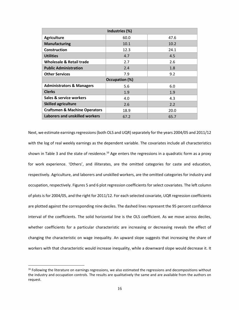
Industries (%)
Agriculture 60.0 47.6
Manufacturing 10.1 10.2
Construction 12.3 24.1
Utilities 4.7 4.5
Wholesale & Retail trade 2.7 2.6
Public Administration 2.4 1.8
Other Services 7.9 9.2
Occupation (%)
Administrators & Managers 5.6 6.0
Clerks 1.9 1.9
Sales & service workers 4.0 4.3
Skilled agriculture 2.6 2.2
Craftsmen & Machine Operators 18.9 20.0
Laborers and unskilled workers 67.2 65.7
Next, we estimate earnings regressions (both OLS and UQR) separately for the years 2004/05 and 2011/12
with the log of real weekly earnings as the dependent variable. The covariates include all characteristics
shown in Table 3 and the state of residence.16 Age enters the regressions in a quadratic form as a proxy
for work experience. ‘Others’, and illiterates, are the omitted categories for caste and education,
respectively. Agriculture, and laborers and unskilled workers, are the omitted categories for industry and
occupation, respectively. Figures 5 and 6 plot regression coefficients for select covariates. The left column
of plots is for 2004/05, and the right for 2011/12. For each selected covariate, UQR regression coefficients
are plotted against the corresponding nine deciles. The dashed lines represent the 95 percent confidence
interval of the coefficients. The solid horizontal line is the OLS coefficient. As we move across deciles,
whether coefficients for a particular characteristic are increasing or decreasing reveals the effect of
changing the characteristic on wage inequality. An upward slope suggests that increasing the share of
workers with that characteristic would increase inequality, while a downward slope would decrease it. It
16 Following the literature on earnings regressions, we also estimated the regressions and decompositions without the industry and occupation controls. The results are qualitatively the same and are available from the authors on request.

17
is important to note that these predictions are based on the assumption that the wage structure, i.e. the
returns to observed worker characteristics, remains intact as the distribution of characteristics changes.
In effect, this amounts to assuming away the presence of general equilibrium effects, a standard
assumption made in this literature.
The first row of plots in Figure 5 show that the coefficients for being male were positive and significant,
implying the presence of a gender earnings gap. The UQR male coefficients were decreasing across
deciles: In 2011/12, the male coefficient value was 0.69 at the first decile, 0.44 at the median, and 0.40 at
the ninth decile. This is termed as the ‘sticky floor’ effect and shows that while men earned more than
women throughout the distribution, the penalty for being female was more pronounced at the bottom of
the distribution.17 The decreasing UQR coefficients also mean that having a greater proportion of men
would reduce earnings inequality among wage earners. This was unambiguously true for 2004/05 as the
coefficients decline monotonically across deciles, and it was true for the lower part of the 2011/12
distribution.
The second through fourth rows of plots in Figure 5 show the presence of caste earnings gaps, though we
do not see such gaps in all parts of the distribution. In 2004/05, the UQR coefficients for ST, SC and OBC
(Other Backward Classes) vis-à-vis ‘Others’, show that there was an earnings penalty for all three groups
at the upper deciles but not at the lower ones.18 In 2011/12, the caste penalty for ST persisted, although,
unlike 2004/05 it was experienced at the lower deciles. Surprisingly, the caste penalty for SC and OBC
disappeared in 2011/12. Interestingly, in the regressions without industry and occupation controls (not
shown here), the caste earnings gap for SC and OBC persisted even for 2011/12. This suggests that in
17 Deshpande et al. (2015) also find a sticky floor for 1999/2000 and 2009/10 among regular salaried workers in India. 18 The ‘Others’ group includes, but is not confined to, the Hindu upper castes as the EUS data do not allow us to isolate the Hindu upper castes. Consequently, this four-way division understates the gaps between the Hindu upper castes and the most marginalized ST and SC groups (Deshpande 2011).

18
2011/12, the caste earnings gaps were overwhelmingly because of occupation and industrial segregation
by caste.
The fifth row of Figure 5 indicates that returns to being married moved from being insignificant at lower
deciles to being positive at upper ones. Thus, if the proportion of married individuals were to increase
earnings inequality among wage earners would increase. Except at the ninth decile in 2004/05, there was
no penalty for being Muslim in both years.
Figure 5: UQR Coefficients for select Covariates, 2004/05 and 2011/12
0
0.2
0.4
0.6
0.8
1 2 3 4 5 6 7 8 9
Male 2004/05
UQR OLS
0
0.2
0.4
0.6
0.8
1 2 3 4 5 6 7 8 9
Male 2011/12
UQR OLS
-0.3
-0.2
-0.1
0
0.1
1 2 3 4 5 6 7 8 9
ST 2004/05
UQR OLS
-0.3
-0.2
-0.1
0
0.1
1 2 3 4 5 6 7 8 9
ST 2011/12
UQR OLS

19
Figure 6 examines coefficients for various education categories vis-à-vis the illiterates. First, there is clear
evidence of positive returns to education. Additionally, in 2004/05, for each education category, there
-0.4
-0.3
-0.2
-0.1
0
0.1
1 2 3 4 5 6 7 8 9
SC 2004/05
UQR OLS
-0.4
-0.3
-0.2
-0.1
0
0.1
1 2 3 4 5 6 7 8 9
SC 2011/12
UQR OLS
-0.2
-0.1
0
0.1
1 2 3 4 5 6 7 8 9
OBC 2004/05
UQR OLS
-0.2
-0.1
0
0.1
1 2 3 4 5 6 7 8 9
OBC 2011/12
UQR OLS
-0.1
0
0.1
0.2
0.3
1 2 3 4 5 6 7 8 9
Married 2004/05
UQR OLS
-0.1
0
0.1
0.2
0.3
1 2 3 4 5 6 7 8 9
Married 2011/12
UQR OLS
-0.2
-0.1
0
0.1
1 2 3 4 5 6 7 8 9
Muslim 2004/05
UQR OLS
-0.2
-0.1
0
0.1
0.2
1 2 3 4 5 6 7 8 9
Muslim 2011/12
UQR OLS

20
was a monotonic increase in returns as we moved up the earnings distribution, with an especially sharp
increase at the ninth decile. This pattern persisted in 2011/12 for all categories except primary and middle:
For instance, the coefficient of ‘college and beyond’ was 0.22 at the first decile, 0.28 at the median and
1.7 at the ninth decile. Thus, educating the illiterate population would increase earnings dispersion.19
Figure 6 also reveals how the impact of education on earnings dispersion changed over time. The profile
of UQR coefficients across deciles was flatter in 2011/12 than what it was in 2004/05 revealing that the
inequality enhancing effect of education weakened over the period. The detailed decomposition of the
structure effect in section 4.3.3 shows this more formally.
Figure 6: UQR Coefficients for Education Categories, 2004/05 and 2011/12
19 This finding for rural India is similar to the evidence presented in Azam 2012a for regular salaried workers in urban India. Using conditional quantile regressions on EUS data for 1983, 1993/94 and 2004/05, he finds that returns to secondary and tertiary education have increased over time and are larger at higher quantiles.
-0.05
0.05
0.15
0.25
1 2 3 4 5 6 7 8 9
Primary & Middle 2004/05
UQR OLS
-0.05
0.05
0.15
0.25
1 2 3 4 5 6 7 8 9
Primary & Middle 2011/12
UQR OLS
-0.2
0
0.2
0.4
0.6
0.8
1 2 3 4 5 6 7 8 9
Secondary 2004/05
UQR OLS
-0.2
0
0.2
0.4
0.6
0.8
1 2 3 4 5 6 7 8 9
Secondary 2011/12
UQR OLS

21
4.3 RIF Decomposition Results
Next we turn to RIF decompositions to understand the factors behind the changes in the real earnings
distribution. We first present the aggregate decomposition followed by the detailed decompositions of
the composition and structure effects.
4.3.1 Aggregate Decomposition of Change in Earnings
Figure 7 shows the results of the aggregate decomposition of the change in the (log) real earnings
distribution at different vigintiles. We present the decomposition based on the counterfactual that relies
on the characteristics of 2004/05 and returns of 2011/12.20 For each vigintile, the total difference in log
real earnings over the period is plotted (solid line). The downward slope of the total difference graph once
20 The results based on the other counterfactual that relies on the characteristics of 2011/12 and returns of 2004/05 are very similar and are available on request.
-0.2
0.2
0.6
1
1.4
1 2 3 4 5 6 7 8 9
Higher Secondary 2004/05
UQR OLS
-0.2
0.2
0.6
1
1.4
1 2 3 4 5 6 7 8 9
Higher Secondary 2011/12
UQR OLS
0
1
2
3
1 2 3 4 5 6 7 8 9
College & Beyond 2004/05
UQR OLS
0
1
2
3
1 2 3 4 5 6 7 8 9
College & Beyond 2011/12
UQR OLS

22
again shows that the lower quantiles experienced a larger percentage increase in earnings than the higher
quantiles.
The total difference is decomposed into the structure (dashed) and the composition effects (dotted). Both
components made significant contributions to the overall increase in earnings over the seven-year period.
The only exception to this is at the nineteenth vigintile (95th percentile), where the structure effect is not
significant. Thus, the contribution of the structure effect to the overall increase in earnings was positive
and much larger than the composition effect at all but the top vigintile.21
Figure 7: The RIF Aggregate Decomposition
21 We also implemented the aggregate decomposition using the Melly’s refinement (Melly 2006) of the Machado-Mata Decomposition (Machado and Mata 2005) and found similar results.
0
0.1
0.2
0.3
0.4
0.5
0.6
0.7
5 10 15 20 25 30 35 40 45 50 55 60 65 70 75 80 85 90 95
Log
earn
ings
ch
ange
Percentiles
Total Change Composition Effect Structure Effect

23
An important conclusion from the decomposition is that most of the decline in inequality occurred
because the returns to characteristics improved a lot more at lower percentiles. In fact, it is clear that
while changing characteristics did lead to an improvement in real earnings throughout the distribution, it
had an inequality increasing effect: The composition effect increased sharply after the eighth decile,
implying that had ‘returns to characteristics’ been held constant over the period, earnings inequality
would have risen.
Table 4 confirms this by decomposing several measures of inequality. The first column shows the
difference between the log of real weekly earnings at the 90th and the 10th percentiles, while the second
and the third columns present the 50-10 and 90-50 differences. The final column gives the Gini values for
real weekly earnings. The third row presents the difference between the years that is to be decomposed.
Aggregate decompositions of all four inequality measures confirm that the structure effect had an
inequality decreasing effect, while the composition effect had an inequality increasing effect. In other
words, had labor market characteristics remained the same in 2011/12 as they were in 2004/05, earnings
inequality would have dropped: e.g., the Gini coefficient would have dropped from 0.461 to 0.389 instead
of the observed Gini of 0.396 in 2011/12. Decompositions of the 90-50 and 50-10 measures reveal that
the inequality increasing effect of the composition effect was mainly coming from changes at the top end
of the wage distribution. This is reflected by the larger contribution of the composition effect on the 90-
50 measure compared to the 50-10 measure.
In summary, the aggregate decomposition of all inequality measures reveals that the decline in inequality
came exclusively from the structure effect, but the detailed decompositions that follows presents a more
nuanced picture.
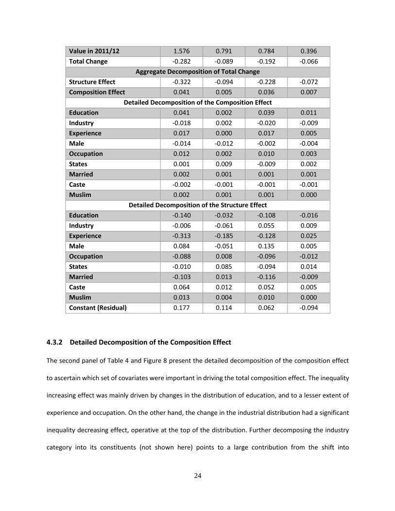
Table 4: Decomposition of Changes in Inequality Measures from 2004/05 to 2011/12
90-10 50-10 90-50 Gini
Value in 2004/05 1.857 0.880 0.977 0.461
24
Value in 2011/12 1.576 0.791 0.784 0.396
Total Change -0.282 -0.089 -0.192 -0.066
Aggregate Decomposition of Total Change
Structure Effect -0.322 -0.094 -0.228 -0.072
Composition Effect 0.041 0.005 0.036 0.007
Detailed Decomposition of the Composition Effect
Education 0.041 0.002 0.039 0.011
Industry -0.018 0.002 -0.020 -0.009
Experience 0.017 0.000 0.017 0.005
Male -0.014 -0.012 -0.002 -0.004
Occupation 0.012 0.002 0.010 0.003
States 0.001 0.009 -0.009 0.002
Married 0.002 0.001 0.001 0.001
Caste -0.002 -0.001 -0.001 -0.001
Muslim 0.002 0.001 0.001 0.000
Detailed Decomposition of the Structure Effect
Education -0.140 -0.032 -0.108 -0.016
Industry -0.006 -0.061 0.055 0.009
Experience -0.313 -0.185 -0.128 0.025
Male 0.084 -0.051 0.135 0.005
Occupation -0.088 0.008 -0.096 -0.012
States -0.010 0.085 -0.094 0.014
Married -0.103 0.013 -0.116 -0.009
Caste 0.064 0.012 0.052 0.005
Muslim 0.013 0.004 0.010 0.000
Constant (Residual) 0.177 0.114 0.062 -0.094
4.3.2 Detailed Decomposition of the Composition Effect
The second panel of Table 4 and Figure 8 present the detailed decomposition of the composition effect
to ascertain which set of covariates were important in driving the total composition effect. The inequality
increasing effect was mainly driven by changes in the distribution of education, and to a lesser extent of
experience and occupation. On the other hand, the change in the industrial distribution had a significant
inequality decreasing effect, operative at the top of the distribution. Further decomposing the industry
category into its constituents (not shown here) points to a large contribution from the shift into

25
construction. The large shift from agriculture to construction noted earlier, decreased earnings inequality.
The greater proportion of male workers, also contributed to the decline in inequality. Changes in the
distribution of state of residence, marital status, caste and religion did not have a major effect on change
in inequality.
Figure 8: Detailed Decomposition of the Composition Effect for select covariates
4.3.3 Detailed Decomposition of the Structure Effect
The bottom panel of Table 4 presents the decomposition of the structure effect. The Gini decomposition
reveals that the education, occupation and the residual (the unexplained portion of the structure effect)
were significant in reducing earnings inequality, while none of the other components were statistically
significant.
As noted earlier (Table 4), the decline in inequality came disproportionately due to the structure effect
and especially from changes at the top of the distribution. The decomposition of the structure effect
component of the 90-50 measure shows that a large part of the change (-0.228) can be explained by
changing returns to education (-0.108) and to occupation (-0.096). As noted in Figure 6, the returns to
-0.05
0
0.05
0.1
0.15
0.2
5 10 15 20 25 30 35 40 45 50 55 60 65 70 75 80 85 90 95
Log
Earn
ings
Ch
ange
Percentiles
Total Experience Education Industry

26
education (with illiterates as the base category) actually declined at the higher end of the wage
distribution, whereas returns did not change significantly in the middle. The same is true for the return
to higher occupations (laborers and unskilled workers as the base category).
5 Conclusions
Using nationally representative data from the Employment Unemployment Survey we examine the
changes in real weekly earnings from paid work for rural India from 2004/05 to 2011/12.
For wage earners who constituted about a quarter of the rural working age population, we find that their
real earnings increased at all percentiles. Using consumption expenditure data that span the entire
population, other studies22 have also documented an improvement in all parts of the distribution. Taken
together, there is clear evidence that economic growth in the post-reform period (after the early 1990s)
has been accompanied by a reduction in poverty.23 At the same time, according to official estimates, in
2011/12, 25.7 percent of the rural population was below the poverty line. This figure represents about
216.7 million poor persons, a large number of people living below a minimum acceptable standard.24
Our analysis also reveals that earnings inequality in rural India decreased over the seven year period, and
about half of the decline can be accounted for by the decline in daily wage inequality. However, while the
rural Gini fell over this period, it remained virtually unchanged in urban India. This shows that the
dynamics of earnings is different for the two sectors. This could be because the underlying structural
characteristics are different, for example, while agriculture is the largest employer in rural India, for urban
22 Kotwal et al. 2011, for all-India, 1983-2004/05; Jayaraj and Subramanian 2015, for rural and urban separately, 2004/05-2009/10. 23 Using NSS data on consumption expenditure from 1957 to 2012, Datt at al (2016) provide direct evidence that growth in India has been accompanied with a decline in poverty, especially after economic reforms were initiated in the early nineties. 24 The corresponding figures for below poverty line population in urban India are: 13.7 percent (53.1 million).

27
India it is services. It could also be the result of different redistributive policies followed in the two sectors.
These aspects need to be recognized when designing future policies to tackle inequality in the two regions.
Aggregate decompositions of the change in inequality measures reveal that the change in returns to
worker characteristics was mainly responsible for the decrease in earning inequality. Further detailed
decompositions reveal that higher levels of education in the population contributed to an increase in
earnings inequality, while lower returns to higher education contributed to a decrease. Rural India also
experienced a construction boom during this period that also contributed to the decrease in earnings
inequality.
Some studies (Datt et al 2016; Thomas 2015) have attributed the tightening of the rural casual labor
market between 2000 and 2012 to the expansion of schooling, and to the construction boom. Others
(Azam 2012; Berg et al. 2015; Imbert and Papp 2015) have found that the MGNREGS (Mahatma Gandhi
National Rural Employment Guarantee Scheme), a large-scale employment guarantee scheme initiated in
rural India in 2005, led to an increase in casual wages.
One cannot be certain that this trend of rising casual wages and declining earnings inequality will continue
into the future. Regardless of the underlying causes of the recent decline in earnings inequality in rural
India, volatility in global crop prices and the drought conditions currently experienced by large parts of
the country because of two consecutive weak monsoons are important reminders that policies designed
to foster employment opportunities and wage growth of unskilled workers outside of agriculture are
crucial for improving the economic well-being of the second part of India.

28
Finally, we end with the caveat that although India has the lowest Gini value among the BRICS countries,25
and we find that earnings inequality declined in rural India between 2004/05 and 2011/12, these facts
mask extreme deprivations and inequities in access to health care, education and physical infrastructure
such as safe water and sanitation (Drèze and Sen 2013). One needs to be cognizant that extreme
inequalities prevail in many other dimensions beyond earnings and consumption expenditure.
6 References
Azam, M. 2012a. “Changes in Wage Structure in Urban India, 1983–2004: A Quantile Regression
Decomposition.” World Development; 40(6): 1135-1150.
Azam, M. 2012b. “The Impact of Indian Job Guarantee Scheme on Labor Market Outcomes: Evidence
from a Natural Experiment” IZA Discussion Papers; IZA DP No. 6548.
Banerjee, A. and T. Piketty. 2005. “Top Indian Incomes, 1922-2000.” World Bank Economic Review;
19(1): 1-20.
Berg, E., S. Bhattacharyya, D. Rajasekhar, and R. Manjula. 2015. “Can Public Works Increase
Equilibrium Wages? Evidence from India’s National Rural Employment Guarantee.”
http://www.erlendberg.info/agwages.pdf.
Blinder, A. 1973. “Wage Discrimination: Reduced Form and Structural Estimates.” Journal of Human
Resources; 8:436-455.
Bound, J. and G. Johnson. 1992. “Changes in the structure of wages in the 1980's: an evaluation of
alternative explanations.” The American Economic Review, 82(3): 371‐392.
Cain, J. S., R. Hasan, R. Magsombol, and A. Tandon. 2010. “Accounting for Inequality in India: Evidence
from Household Expenditures.” World Development; 38(3): 282-297.
25 According to estimates from the World Bank, the Gini values for BRICS countries are as follows: Brazil-0.539 (2009); Russia-0.397 (2009); India-0.339 (2009); China-0.421 (2010) and South Africa-0.630 (2008). These are available at http://data.worldbank.org/indicator/SI.POV.GINI. Last accessed on November 18, 2015.

29
Datt, G., M. Ravallion, and R. Murgai. 2016. “Growth, Urbanization, and Poverty Reduction in India.”
World Bank Group, Policy Research Working Paper 7568.
Deshpande, A. 2011. “The Grammar of Caste: Economic Discrimination in Contemporary India.”
Oxford University Press, New Delhi.
Deshpande, A., D. Goel, and S. Khanna. 2015. “Bad Karma or Discrimination? Male-Female Wage
Gaps among Salaried Workers in India.” IZA Discussion Papers, IZA DP No. 9485.
Drèze, J. and A. Sen. 2013. “An Uncertain Glory: India and its Contradictions.” Princeton University
Press.
Dutta, P. V. 2005. “Accounting for Wage Inequality in India.” Poverty Research Unit at Sussex, PRUS
Working Paper No. 29.
Firpo, S., N. M. Fortin, and T. Lemieux. 2009. “Unconditional Quantile Regressions.” Econometrica;
77: 953–973. doi: 10.3982/ECTA6822
Fortin, N. M., T. Lemieux, and S. Firpo. 2011. “Decomposition Methods in Economics.” Handbook of
Labor Economics (edited by Ashenfelter and Card.); Volume 4A, Chapter 1.
GOI. 2015. “Economic Survey 2014-15.” Government of India, Ministry of Finance.
Goldberg, P. K. and N. Pavcnik. 2007. “Distributional Effects of Globalization in Developing Countries.”
Journal of Economic Literature; Vol XLV: 39-82.
Hnatkovska, V. and A. Lahiri. 2013. “Structural Transformation and the Rural-Urban Divide.” Working
Paper, International Growth Center, London School of Economics.
Imbert, C. and J. Papp. 2015. “Labor Market Effects of Social Programs: Evidence from India's
Employment Guarantee.” American Economic Journal: Applied Economics; 7(2):233-263.
Jacoby, H. and B. Dasgupta. 2015. “Changing Wage Structure in India in the Post-reform Era: 1993-
2011.” Policy Research Working Paper 7426, World Bank.

30
Jayaraj, D. and S. Subramanian. 2015. “Growth and Inequality in the Distribution of India’s
Consumption Expenditure: 1983-2009-10.” Economic and Political Weekly; 50(32).
Katz, L. F. and K. M. Murphy. 1992. “Changes in Relative Wages, 1963‐1987: Supply and Demand
Factors.” The Quarterly Journal of Economics, 107(1): 35‐78.
Kijima, Y. 2006. “Why did wage inequality increase? Evidence from urban India 1983–99.” Journal of
Development Economics; 81: 97-117.
Koenker, R. and G. Bassett. 1978. “Regression Quantiles.” Econometrica; 46: 33- 50.
Kotwal, A. and A. R. Chaudhuri. 2013. “Why is Poverty Declining so Slowly in India?” Ideas for India,
http://www.ideasforindia.in/article.aspx?article_id=110
Kotwal A., B. Ramaswami, and W. Wadhwa. 2011. “Economic Liberalization and Indian Economic
Growth: What's the Evidence?” Journal of Economic Literature; 49(4): 1152-1199.
Krueger, D. and F. Perri. 2006. “Does Income Inequality Lead to Consumption Inequality? Evidence
and Theory.” Review of Economic Studies; 73(1): 163–93.
Machado, J. F., and J. Mata. 2005. “Counterfactual Decomposition of Changes in Wage Distributions
Using Quantile Regression.” Journal of Applied Econometrics; 20: 445–465.
Melly, B. 2006. “Estimation of Counterfactual Distributions using Quantile Regression.” University of
St. Gallen, Discussion Paper.
Motiram, S. and V. Vakulabharanam. 2012. “Indian Inequality: Patterns and Changes, 1993 – 2010.”
India Development Report, Oxford University Press, Vol 7: 224-232.
NFHS. 2009. “Nutrition in India. National Family Health Survey (NFHS-3) India 2005-06.” Ministry of
Health and Family Welfare, Government of India.
Oaxaca, R. L. 1973. “Male-Female Wage Differentials in Urban Labor Markets.” International
Economic Review; 14: 693-709.

31
Planning Commission. 2014. “Report of the Expert Group to Review the Methodology for
Measurement of Poverty.” Planning Commission, Government of India.
RBI. 2015. “Handbook of Statistics on the Indian Economy 2014-15.” Reserve Bank of India.
Sen, A. and Himanshu. 2004. “Poverty and Inequality in India: II: Widening Disparities during the
1990s.” Economic and Political Weekly; 39(39): 4361-4375.
Thomas, J.J. 2015. “India’s Labour Market during the 2000s: An Overview.” Chapter in Ramaswamy,
K.V (ed.), Labour, Employment and Economic Growth in India, Cambridge University Press, New Delhi