Embed Size (px)
Citation preview
Growth, Inequality, and Poverty
in Rural China
The Role of Public Investments
Shenggen FanLinxiu ZhangXiaobo Zhang
RESEARCHREPORT 125INTERNATIONAL FOOD POLICY RESEARCH INSTITUTEWASHINGTON, D.C.
���������� ������������������������������������������������������
�������������������� �����������!�������"����������������� �
!����#��!����������������������������������������������
����������$�����������������
�����������������������������������
� %%&����'()
)��������'*�� +,- �
.-,� �,/+�,0+
!!!����������
�������������� ��������������������������������
���'��������
1��!�'���2�����'���������������������3���������� ���
���������4�����������'5��"��6����'7��� �6�����
�����89������������������:-�0;
��<( ,/=+�=,-�/,+9� #�3��#������;
-��� ������������8������������������������8������
%�����������8�����8�������8>����������������?������
����81��������������8��������6����'5��"������6����'7��� ��
����@�����A��������������9�����������������������������
������;:-�0�
B�?% ��/%�%+� �
%%/�-′/0-8���- � � CC-C
Contents
@� ��� ��
������� �
����!��� ��
��#��!�������� ����
������� �"
-� ���������� -
�� 1��!�'���2�����'��������� %
%� �� �������������������� -/
?� ��������������!��#���D���� �0
0� *��'>�������'��������� %+
+� ����������� ?=
�������"�3D�E��D������������������������������������ 0%
�������"<3������������������������������������ 0?
�������"�3����������*����������� ����������� 00
<� ��������� +C
iii
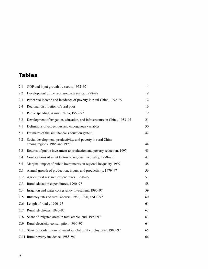
Tables
��- 1*� ����������!� ������'-=0�F=C ?
��� *������������������������������'-=C/F=C =
��% ����������������������������������������������'-=C/F=C -�
��? ������������� ��������������� -+
%�- �� �����������������������'-=0%F=C -=
%�� *��������������������'��������'����������������������'-=0%F=C �-
?�- *������������"������������������������� ��� %
0�- >����������������������2���������� ?�
0�� ����������������'����������'���������������������
������������'-=/0���-==+ ??
0�% ���������� ��������������������������������������'-==C ?0
0�? ����� �����������������������������2�����'-=C/F=0 ?C
0�0 D���������������� �������������������������2�����'-==C ?/
��- ���������!������������'�����'�������������'-=C=F=C 0+
��� ��������������������"���������'-== F=C 0C
��% ��������������"���������'-== F=C 0/
��? ������������!����������������������'-== F=C 0=
��0 ���������������������� �����'-=//'-== '���-==C +
��+ 5�����������'-== F=C +-
��C ��������������'-== F=C +�
��/ ���������������������������� ������'-== F=C +%
��= ������������������������'-== F=C +?
��- ������������������������������������������'-=/ F=C +0
��-- ��������������������'-=/0F=+ ++
iv
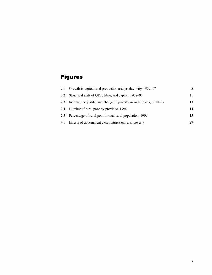
Figures
��- 1��!������������������������������������'-=0�F=C 0
��� ��������������1*�'�� ��'���������'-=C/F=C --
��% ������'���2�����'�����������������������������'-=C/F=C -%
��? (�� ������������� ���������'-==+ -?
��0 ���������������������������������������'-==+ -0
?�- >�����������������"���������������������� �=
v
Foreword
M��� ���������� �������� ������������ ���� ����� ����� �� �� ��� �� �����,
����������������@��������'��������������������������������������
������@���������������������������������������������������������
���������������������������������B�!����'���� ������������������"��������
�������� ����������������������������� ��������2��������������������,
���������������������������������������������������#���������!����
������������!������������
������������������'�����������'5��"��6����'���7��� �6�������!������,
��������������������������������������!�'�����������'��������������2�������,
�����������������������$��������������,������������������������������'��
�����������������������������������#���!����������������������������
�����������������������@������������� �������������������������������",
�������������������������������������������9�G*'���������'��������'���������,
���'������,��������������'�������������������� �!������!��������������
��������������������2�����������������!�����������H��������������������������
��������������������
@�����������������������������������������������������������������,
����������������!�'!���� ������������ ���� �� ���������� ��������������
������������������������������������������������!����� �������������������,
�������@�������������������������������������������!�'�����������������
�� ���� �������� ����������,�������� ��������' ���� �� ������������G*' � ��������
���������������'�����������������������������������' ������������1�����,
����"�������������������������������������������� ������������������,
���������2�������������������������� �������������������������������������
�����������������������������������������2��������������5�#���������'��
����������������� ����������������������������!�������������������������
������������������������������������
1����������������������������������������������������������������,
����������!��<�����I������������������������������������������������ ��
����������� ���!� ��� ������ ��������� B�!����' ��#��� ������ ��������� ��������
������������ ����������������������������������������������������������@����!
�����������,����������������������������������� ��������������������
�������������������������������������������������������'�����������������
���"���H�������������2�������������'����������������� ����������!��,
���������9������������������;�
vi

@�������������������������E�����������������������������������������
������9�����;������������������������ ������������@�������� �����������!��
�������������!��#�������!����A��(�����@�������'����������������������
����������,��������
*������1������
vii
Acknowledgments
T ����������#��!�������������������������� ������������������������,��,
����������������������������������(������(�����������������������)�
���#����B�H���������������������' �������������������'������������,
���!��������������������������������������������D������������������,
���������������������������������9�����;����������������� ���������������,
�������'���������������������'D��#��������'J���������'*���������'���B���5K�,
����������H���������!�������������'�����������'����������������#�� ������,
���,�,�������������������!����!���������������1���������������������������,
���������������������� ����
viii
Summary
C���� �������� !���� ����!� �� �������� �� ����� ������ ������ �� ��� !�
�������' ������ �� ��� �� ���!��!� �� ������ ��������� ����� ���� � ���
���������������������������������������������'�����������2����������
�������������������������������'����� �������������������������L�'�������I�
�������������������!'��� ��������������������������������2������������
B�!�������������� �������������������'������������� �����������������'�
���������!�!����'����������'����������������������������2�����'������
�� ����� ���������������������������@�������������������������������������� ,
��� ��������� �������������!����������������������������� ���2����� �� �����
����������������������������������������������������������������������
$��������������,�������� ���-=C F=C' �� �������������� ������������2������
����������������������������������������������"���������@���������
�������#��������������������� �����������������!�'���2�����'���������' �
��������#����������������������������������������������@���������������
������ � ��� ��� ��������#��� � ����� �� ����������� �� !��# ���#� �� �� ������,
��������������
@�����������!�����������I����������,������������������'�����������������
�������� ��� ���������� 9�G*;' ���������' ����� ��������' ��� ������������ 9���������
�����' ���������' ��� ����������������; ����� ��� �� ���� � ����������� ���������
���!�' �����������������������������������������2������<�����������������,
������� ����������������������������� ��������������'��!�������������������
<����������������������-==C��������������������������������'!�
������������������������������������������������!������������������������
�����������������������������������������������2������@����������!��������,
�����������������!������������������������������H�������������������
��������������'������������������������������������������ ���
1���������"��������������������� �� ������ ����� ���������������������
��������������2�������������������������������������!�����������������������
���������!��������� ��������������������,������2�����,��������������1��,
������ �������� �� ����������� �G* �� �������� �������� ����������� ���������� ��
���'���������"�������������������������������������������������!�'!����
�����������������������������������������������������������������������
<�������������������������������!��������#�����!��������������@��������,
������������������������������������������G*�������� ���#������������ �
������������������������1�����������������������������������9�����'���������'
�������������������;����� ���������������������������������2�������!���'
ix
�!�����������������������������������������������������������������!�����
��������������������������������������������������������������!��������
����������������������������2�����'�����������#��,��!� ������!�������!������
� ���#��� ������� �� �� ������� ����� �� ������������ ������ ��������� ���,������
�����������'��������,������������������������!������������������������,
���������������������������������
*�������������������������������������������������'���������������������
��������' ������ � ��������� �� ������ �������� !��� ������ �� �� !����� ������'
!�����������������������������������!�!���������������������������������
���� �� ��������� ����������' ��� ��� ���� �� ��������� ��������' ��������� �� ��
!����� ������ ��� � �� ������ ��������� �� �������� ���2�����' !���� ��������� ��
��������������������������!����������"���������������������2��������
@���������������������������������������������������������������������
��������������������������������������������������!�'�����������������
�� ���� �������� ����������,�������� ��������' ���� �� ������������G*' � ��������
���������������'�������������������������������'�����������������������'���,
����������������������������������������������������!���������<�����
������������������������� ����������������!���������������������������
(� ��� �������� �� ����� ��� ������� ������ �� ������� ��� ������ ������ � ��
������������������������������������<���#������������������������������
�������� ���������������������������������������������������������������@����!
�����������,����������������������������������� ��������������������
���������������������������
�������������������������'��������������������"���H�������,������2�����,
��������������'����������������� ����������!�����������9��������������
����;� B�!����' � ��"���H� ������ � �������� �� ����������� ���������' ��������
������ �����������������������
�������������������������������������,�2���� ������������������H����������
��������� ���������������!�����������'��!��������� ��������������2������
������' �����I� ���� ��� �� )���� @���� M�����H���� 9)@M; ����� ��� ���� ��������
����!�� ��� ����������� ������������������� ��������� �������@����������'
��������'����������������������� �������������������������������� � ���
��������������������������������������������������� ������������'��������������
����������������
x
C H A P T E R 1
Introduction
China is one of the few countries in the developing world that has made progress in
reducing its total number of poor during the past two decades (World Bank 2000).
Numbers of poor in China fell precipitously, from 260 million in 1978 to 50 million
in 1997.1 A reduction in poverty on this scale and within such a short time is unprecedented
in history and is considered by many to be one of the greatest achievements in human devel-
opment in the twentieth century.2 Contributing to this success are policy and institutional
reforms, promotion of equal access to social services and production assets, and public
investments in rural areas.
The literature on Chinese agricultural growth, regional inequality, and rural poverty re-
duction is extensive. But few have attempted to link these topics to public investment.3 We
argue that even with the economic reforms that began in the late 1970s it would have been im-
possible to achieve rapid economic growth and poverty reduction without the past several
decades of government investment. Prior to the reforms, the effects of government investment
were inhibited by policy and institutional barriers. The reforms reduced these barriers, en-
abling investments to generate tremendous economic growth and poverty reduction. Similarly,
public investment may have played a large role in reducing regional inequality, an issue of in-
creasing concern to policymakers.
China’s experience provides important lessons for other developing countries. In the gen-
eral literature on public economics, the rationale behind government spending is to spur effi-
ciency (or growth) by correcting market failures. Examples of such failures are externalities;
scale economies; failures in related markets like credit, insurance, and labor; nonexcludabil-
ity; and incomplete information about benefits and costs. Less attention is paid to the role of
1Unlike in many other developing countries, poverty in China has mainly been limited to rural areas. Urban
poverty incidence is extremely low, although there has been a slight increase recently (Piazza and Liang 1998).
The number of rural poor for each year is reported in the China Agricultural Development Report, a white paper
of the Ministry of Agriculture. The poverty line is defined as the level below which income (and food produc-
tion in rural areas) are below subsistence levels for food intake, shelter, and clothing.
2Even if the international standard of one dollar per day measured in purchasing power parity is used, China’s
poverty reduction is still remarkable when compared with other countries, having declined from 31.3 percent in
1990 to 11.5 percent in 1998. Using the same poverty line, the incidence of poverty in South Asia declined only
from 45 percent in 1987 to 40 percent in 1998, while for Africa as a whole incidence changed very little, from
46.6 percent in 1987 to 46.3 percent in 1998 (World Bank 2000).
3Some studies link public investment to food security and agricultural growth (Fan and Pardey 1992; Huang,
Rosegrant, and Rozelle 1997; Huang, Rozelle and Rosegrant 1999; Fan 2000). But very few link these invest-
ments to poverty reduction in a systematic way. Chapter 4 presents a more detailed literature review.
1
public investment in pursuing equity or
poverty alleviation objectives. Many neo-
classical economists favor solving poverty
problems by using welfare redistribution
means, for example, by taxing the rich and
transferring income directly to the poor. But
few countries, particularly developing
countries, have succeeded in solving the
poverty problem solely through direct in-
come transfers. Therefore, more govern-
ments are now convinced that poverty and
inequality may be more effectively reduced
by promoting the income-generation capac-
ity of the poor. Effective public spending
policy is one of the instruments used to
achieve this.
Because many developing countries are
undergoing substantial macroeconomic ad-
justments and facing tight budgets, it is crit-
ical to analyze the relative contributions of
various expenditures to growth and poverty
reduction. Valuable insights can thus be
gained to further improve the allocative ef-
ficiency of limited, even declining, public
resources.
The primary purpose of this study is (1)
to develop an analytical framework for ex-
amining the specific role of different types
of government expenditure on growth, re-
gional inequality, and poverty reduction by
controlling for other factors such as institu-
tional and policy changes and (2) to apply
that framework to rural China.
Using provincial-level data for the past
several decades, we construct an economet-
ric model that permits calculation of eco-
nomic returns, the number of poor people
raised above the poverty line, and impact on
regional inequality for additional units of
expenditure on different items. The model
enables us to identify the different channels
through which government investments af-
fect growth, inequality, and poverty. For in-
stance, increased government investment in
roads and education may reduce rural
poverty not only by stimulating agricultural
production, but also by creating improved
employment opportunities in the nonfarm
sector. Understanding these different effects
provides useful policy insights to improve
the effectiveness of government poverty al-
leviation strategies.
Moreover, the model enables us to cal-
culate growth, inequality, and poverty-re-
duction effects from the regional dimen-
sion. Specific regional information helps
government to better target its limited re-
sources and achieve more equitable re-
gional development, a key objective de-
bated in both academic and policymaking
venues in China.
The rest of the report is organized as fol-
lows. Chapter 2 details the evolution of
growth, inequality, and poverty in rural
China over the past several decades. Chap-
ter 3 describes trends of public investment
in technology, education, and infrastructure,
as these have long-term effects on growth,
poverty reduction, and income distribution.
Chapter 4 develops the conceptual frame-
work to track multiple poverty effects of
public investment. Chapter 5 describes the
data and estimation strategy and presents
the estimation results. Chapter 6 concludes
the report with policy implications and fu-
ture suggested research directions.
2 CHAPTER 1
C H A P T E R 2
Growth, Inequality, and Poverty
T his chapter examines trends in growth, inequality, and poverty, as well as associated
changes in institutions and policies. It thus provides a background for analysis in later
chapters of how various public investments affect growth, inequality, and poverty.
Macroeconomic Reforms
The dynamic growth of the Chinese economy over the past 50 years ranks among the most
important developments of the twentieth century. China has experienced a number of policy
and institutional reforms, some of which have involved abrupt dislocations of the country’s
economic, social, cultural, and political order. The official raison d’être for these reforms was
to promote rapid economic development and a more equal distribution of wealth, to attain
national self-sufficiency, and to further socialist or communist ideals. Two distinct stages are
normally used in describing the development of the national economy: adoption and imple-
mentation of a Soviet-type economy from 1952 to 1977 and gradual economic reform toward
a market-led economic system since 1978.
Prior to 1978, China faced a hostile international environment with political isolation and
economic embargoes. Political leaders adopted a heavy industry-oriented development strat-
egy to catch up with developed western countries. This approach is clearly stated in China’s
first five-year plan (1952–57) (Lin, Cai, and Li 1996).
To guarantee low production costs for the heavy industry sector, agricultural product prices
were suppressed to subsidize the cost of living of urban workers. The government also estab-
lished the hukou system of household registration in this period, confining people to the vil-
lage or city of their birth in order to ensure enough agricultural laborers to produce grain for
urban workers. This urban-biased policy created a large gap in income and standard of living
between rural and urban residents 1982–2000 (SSB, various years).
The state or collectives owned production assets, and all firms produced products in
accordance with government plans and quotas. Prices of both inputs and outputs were strictly
controlled by government without regard for market demand and supply. Allocation of inputs
among firms and products among consumers was also based on government plan rather than
on market signals. Workers earned a fixed monthly salary or an amount based on their work-
ing hours, often without consideration of their work efforts. All these policies led to an egali-
tarianism within rural areas and within cities, despite the large gap between them.
In spite of the counterproductive economic policies, the Chinese economy did exhibit
some important accomplishments during 1952–77. Foremost of these was a record of impres-
sive economic growth. From 1952 to 1977, China’s GDP grew at an average annual rate of
5.93 percent (Table 2.1). However, due to the obligatory savings inherent in the Soviet-type
3
growth strategy, personal consumption
grew at only 2.2 percent per annum during
the same period. The result was extremely
low living standards for the general popula-
tion, rural residents in particular.
Chinese economic reforms began in the
rural areas in 1978 (more details are in-
cluded in the next section). Urban-sector
reforms did not begin formally until 1984,
before which some reforms were enacted
piecemeal. But even after 1984, the reform
package was far from the “big bang” pro-
grams then being advocated for Eastern
Europe and the former Soviet Union. In
particular, China’s urban-sector reforms
emphasized expansion of enterprise and
local autonomy and incentives and the
reduction—but not elimination—of within-
plan allocations (Groves et al. 1994).
In addition, China gradually opened its
economy to foreign trade and investment,
which not only contributed directly to rapid
economic growth but also helped to restruc-
ture the national economy. In the urban in-
dustrial sector, markets for most industrial
products replaced the planned allocation of
goods. In other words, state-owned enter-
prises were forced to operate according to
market rules. Furthermore, non-state enter-
prises, both domestic and foreign, could be
created and could compete with state-
owned enterprises in these markets.
In terms of government fiscal and finan-
cial policies, which are directly relevant to
our study, the government decentralized its
management system by granting localities
greater flexibility in collecting revenue and
making expenditure decisions. This greatly
increased incentives for local governments
to develop their economies so as to retain
more revenue for improving local infra-
structure and human capital. Due to the
regions’ differing tax bases, the trend of
decentralization might have affected the
4 CHAPTER 2
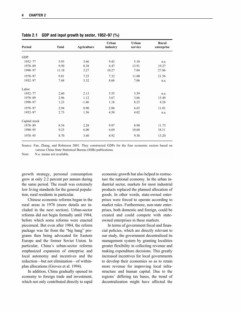
Table 2.1 GDP and input growth by sector, 1952–97 (%)
Urban Urban Rural
Period Total Agriculture industry service enterprise
GDP
1952–77 5.93 3.66 9.43 5.10 n.a.
1978–89 9.50 8.38 6.47 13.91 19.27
1990–97 11.18 5.27 10.27 7.04 27.86
1978–97 9.81 7.25 7.32 11.00 21.56
1952–97 7.68 5.32 8.66 7.06 n.a.
Labor
1952–77 2.60 2.13 5.55 3.59 n.a.
1978–89 2.96 1.12 3.67 3.66 15.49
1990–97 1.23 –1.46 1.18 8.25 4.26
1978–97 2.94 0.90 2.86 6.65 11.01
1952–97 2.73 1.56 4.50 4.02 n.a.
Capital stock
1978–89 8.54 2.28 9.97 8.90 11.75
1990–95 9.25 6.00 6.69 10.60 18.11
1978–95 8.70 3.40 8.92 9.38 13.20
Source: Fan, Zhang, and Robinson 2001. They constructed GDPs for the four economic sectors based on
various China State Statistical Bureau (SSB) publications.
Note: N.a. means not available.
level of public expenditures across regions,
therefore perhaps leading to differential
rates of growth and poverty reduction.4
As a result of the reform policies, na-
tional GDP grew at about 10 percent per
annum from 1978 to 1997 (Table 2.1). Per
capita income increased more than fourfold,
or 7.8 percent per annum. The overall living
standard of the Chinese population and na-
tional development indicators improved at
an unprecedented rate, approaching those
in many middle-income countries (World
Bank, World Development Report 2000).
Policy Reforms andAgricultural Growth
This section reviews major institutional
changes and policy reforms in rural areas
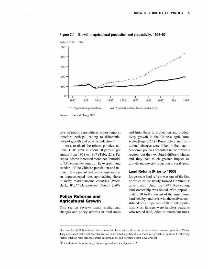
and links these to production and produc-
tivity growth in the Chinese agricultural
sector (Figure 2.1).5 Rural policy and insti-
tutional changes were linked to the macro-
economic policies described in the previous
section, but they exhibited different phases
and they had much greater impact on
growth and poverty reduction in rural areas.
Land Reform (Prior to 1953)Large-scale land reform was one of the first
priorities of the newly formed Communist
government. Until the 1949 Revolution,
land ownership was feudal, with approxi-
mately 70 to 80 percent of the agricultural
land held by landlords who themselves con-
stituted only 10 percent of the rural popula-
tion. Most farmers were landless peasants
who rented land, often at exorbitant rates,
GROWTH, INEQUALITY, AND POVERTY 5
Figure 2.1 Growth in agricultural production and productivity, 1952–97
Source: Fan and Zhang 2001.
4Lin and Liu (2000) analyzed the relationship between fiscal decentralization and economic growth in China.
They concluded that fiscal decentralization contributed significantly to economic growth, in addition to other key
factors such as rural reform, capital accumulation, and nonstate sector development.
5 For milestones in reforming Chinese agriculture, see Appendix A.
from these landowners. Soon after 1949,
land was confiscated by the government
without compensation and redistributed to
peasant farmers. By the end of 1952 the
land reform was successfully accomplished
(Ministry of Agriculture 1989).
Collectivization (1953–56)Beginning in 1952, some small-scale peas-
ant farmers voluntarily pooled their land and
other resources into a cooperative mode of
operation. At first, farmers were free to join
or leave the cooperatives without penalty.
Government efforts to develop large col-
lective operations soon followed, and by
1956 most of China’s agricultural produc-
tion was done on a collective basis (Lin
1990; Putterman 1990). Under this system,
land ownership was vested in a collective
that usually consisted of some 200 families.
Within the collective, an individual’s in-
come was tied to the number of work points
accumulated throughout the year in relation
to the time, effort, skill, and political attitude
the laborer brought to the collective work.
Households also farmed home gardens on
“private plots,” which then constituted about
5 percent of all arable land. Produce from
these gardens could be sold on free markets
(Ministry of Agriculture 1989). All these
policies led to rapid growth in both produc-
tion and productivity, with annual growth
rates of 5.3 percent and 2.7 percent, respec-
tively (Fan and Zhang 2001).6
Great Leap Forward andCommunization (1957–60)Beginning in 1958, the central government
promoted an even larger scale of production
in agriculture. Advanced cooperatives were
merged into communes. The forced rapid
collectivization gave farmers no incentives
to increase production and productivity,
since their income and well-being was no
longer linked to their work efforts. At the
height of the commune movement in
1958–59, the average communal unit had
grown to 5,000 households covering 10,000
acres, and food was allocated as much on
the basis of need as on accumulated work
points. The communes owned virtually all
production means except for agricultural
labor. The government, through its adminis-
tration and procurement systems, rigidly
controlled both quantity and price of out-
puts and inputs. Commune leaders made
production decisions, with the role of farm-
ers limited to supply of labor for commune
production. Work on private plots was also
prohibited. As a result, both agricultural
production and productivity declined
sharply, by 6 percent and 5 percent per
annum, respectively (Figure 2.1). The wide-
spread drought and flood in most of China
in 1959 worsened the devastating situation.
An estimated 30 million people died of star-
vation, one of the largest human tragedies
in history (Lin 1990; Lin and Yang 2000).
Economic Adjustments(1961–65)The Great Famine (1959–61) led the gov-
ernment to implement an adjustment and
consolidation policy after 1961. Production
was decentralized into smaller units called
“production teams,” a sub-unit of the com-
mune consisting of only 20 to 30 neighbor-
ing families. By 1962, production teams
were the basic unit of operations and
accounting in most rural areas. Decisions
6 CHAPTER 2
6 The growth rates of agricultural production and productivity used here are new measures constructed by Fan
and Zhang (2001). They adjusted livestock and fishery output data to measure growth in output, input, and total
factor productivity for Chinese agriculture based on detailed quantity and price information. Fan and Zhang
found that official statistics overestimate both aggregate output and input, resulting in biased estimates of total
factor productivity growth. Furthermore, the official data overstates the impact of the rural reforms on both pro-
duction and productivity growth. Nevertheless, both production and productivity still grew at respectable rates
during the reform period.
on farm operations, including the adoption
of new technologies, were primarily made
by team leaders (MOA 1989). Production
and productivity recovered rapidly, grow-
ing at more than 9.0 percent and 4.7 percent
per annum, respectively (Figure 2.1).
Cultural Revolution(1966–76)During the Cultural Revolution of 1966–76,
production and productivity growth were
again depressed by policy failures. The
government reinstated many controls that
were loosened during the three-year adjust-
ment period of 1962–65. Although produc-
tion was still organized in the smaller unit
production teams, it was nonetheless tightly
controlled by government. Farmers’ in-
comes were not closely related to their pro-
duction efforts. The government controlled
virtually all input and output markets. No
market transactions of major agricultural
products were allowed outside the procure-
ment system. Market exchanges of land be-
tween different production units in the col-
lective system were also outlawed. Because
farmers had few incentives, inefficiency
was rampant in agricultural production.
Production during this period grew at 2.6
percent per annum, and there was virtually
no gain in total factor productivity.
The First Phase of Reform(1979–84)Due to the more than two decades of poor
performance of the agricultural sector, cen-
tral government decided to reform the rural
areas in 1978. These reforms occurred in
two reasonably distinct phases. The first
phase focused on decentralizing the system
of agricultural production, while the second
phase emphasized liberalizing factor and
output markets.7
During the initial phase of the reforms,
the state raised its procurement prices for
agricultural products and reopened rural
markets for farmers to trade produce from
their private plots. After two years of ex-
periments, in 1981 the government began to
decentralize agricultural production from
the commune system to individual farm
households. By 1984, more than 99 percent
of production units had adopted the house-
hold production responsibility system.
Under the system, farmers were free to
make production decisions based on market
prices as long as they fulfilled government
procurement quotas for grains. Land was
still owned by the collectives, but use rights
could be transferred.
In addition to decentralization of the pro-
duction system, government began to reform
the agricultural procurement system. Prior
to 1984, virtually all commodities were
subject to various government procurement
programs. In 1984, the number of com-
modities within the government procure-
ment system was gradually reduced, from
113 to 38 (Ministry of Agriculture 1989).
Unsurprisingly, both technical efficiency
(from the decentralization of the production
system) and allocative efficiency (from
price and marketing reforms) increased sig-
nificantly during this first phase of reforms.
Production increased by more than 6.6 per-
cent and productivity by 6.1 percent per
annum from 1979 to 1984 (Figure 2.1).
The Second Phase Reform(1985–89)The second phase of reforms was designed
to further liberalize the country’s (agricul-
tural) pricing and marketing systems. How-
ever, the government cut the marginal
(above-quota) procurement price for grain
in 1985. Meanwhile, input prices increased
GROWTH, INEQUALITY, AND POVERTY 7
7Various studies attempt to assess the impact of this reform on production growth (McMillan, Whalley, and Zhu
1989; Fan 1990, 1991; Lin 1992; Zhang and Carter 1997; Fan and Pardey 1997; Huang, Rosegrant, and Rozelle
1997). All found that during this initial stage of reform, institutional and market reform was the major source of
productivity growth.
much faster than the government’s output
procurement prices, raising production
costs.8 The result was an end to the rapid
output growth of the previous five years.
Annual production grew at only 2.7 percent
during this second phase of reforms, and
there were no significant productivity gains
(Figure 2.1).
New Developments in AgriculturalPolicy (1990–Present)The 1990s marked a new development
stage in Chinese agriculture.9 The govern-
ment continued to implement market and
price reforms, and it further reduced the
number of commodities under the govern-
ment procurement system. The number of
commodities subject to state procurement
programs declined from 38 in 1985 to only
9 in 1991. In 1993, the grain market was
further liberalized, and the grain ration-
ing system that had been in existence for
40 years was abolished. In 1993, more
than 90 percent of all agricultural produce
was sold at market-determined prices, a
clear indication of the degree to which
China’s agriculture had been transformed
from a command-and-control system to a
largely free-market one. To increase farm-
ers’ incomes, government increased its
procurement prices for grains by 40 per-
cent in 1994. In 1996, it increased pro-
curement prices 42 percent further. As a
result, agricultural production and produc-
tivity continued to rise rapidly with growth
rates of 3.8 percent and 2.3 percent per
annum, respectively, from 1990 to 1997
(although these were lower than during the
first phase of the reforms).
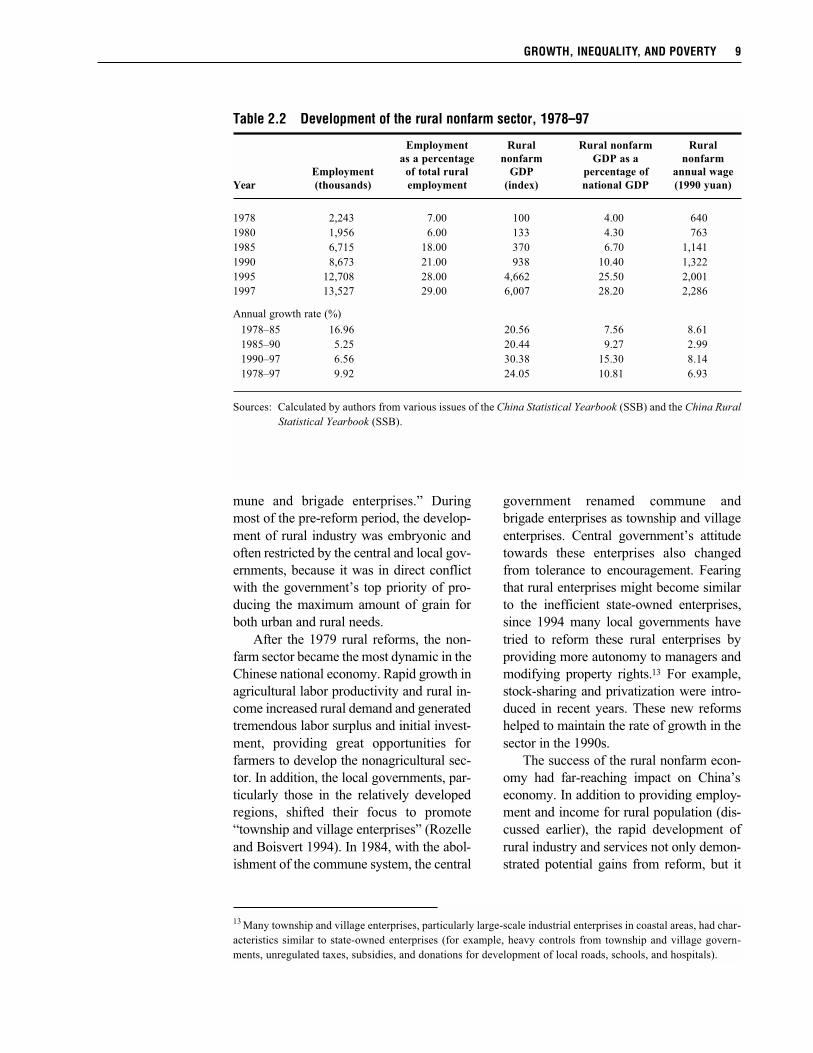
Rural Nonfarm SectorOne of the most dramatic changes in rural
China has been the rapid increase of rural
enterprises during the past two decades.10
Employment in the nonfarm sector as a per-
centage of total rural employment grew
from 7 percent in 1978 to 29 percent in
1997 (Table 2.2). By 1997, rural enterprise
accounted for more than a quarter of na-
tional GDP. Yet this sector was almost non-
existent even as late as 1978. In 1997, GDP
produced by rural industry in China was
larger than the GDP of the entire industrial
sector of India.11 Without development of
the rural nonfarm sector, annual GDP
growth in China from 1978 to 1995 would
have been 2.4 percent lower per annum.
The rapid development of the rural non-
farm sector not only contributed to rapid
national GDP growth, but also raised the
average per capita income of rural residents.
In 1997, more than 36 percent of rural in-
come was from rural nonfarm activities
(SSB 1998), while rural income in 1978 was
predominantly from agricultural production.
The rural nonfarm sector developed in
several stages. The first can be traced back
as far as 1958, when communes set up
many small-scale industrial enterprises (for
example, steel mills), all of which failed im-
mediately.12 During the nationwide agricul-
tural mechanization drive of the early
1970s, rural small-scale industrial enter-
prises reemerged. Most of these started as
agricultural machine repair shops and food-
processing mills. Many enterprises in the
urban hinterlands soon became subcontrac-
tors of state-owned enterprises. These com-
munity enterprises were known as “com-
8 CHAPTER 2
8 The rising cost of production was reported by the Ministry of Agriculture in its Production Cost Survey
(various years).
9Huang, Lin, and Rozelle (1999) provide a good summary of Chinese agricultural policies since the 1980s.
10 Qian and Jin (1998), Chen and Rozelle (1999), Lin and Yao (1999), and Oi (1999) discuss the development of
rural enterprise and its contribution to the Chinese economy from different angles.
11Calculated by the authors using data from the World Bank’s World Development Report 2000.
12This is largely due to the national industrialization drive during the Great Leap Forward.
mune and brigade enterprises.” During
most of the pre-reform period, the develop-
ment of rural industry was embryonic and
often restricted by the central and local gov-
ernments, because it was in direct conflict
with the government’s top priority of pro-
ducing the maximum amount of grain for
both urban and rural needs.
After the 1979 rural reforms, the non-
farm sector became the most dynamic in the
Chinese national economy. Rapid growth in
agricultural labor productivity and rural in-
come increased rural demand and generated
tremendous labor surplus and initial invest-
ment, providing great opportunities for
farmers to develop the nonagricultural sec-
tor. In addition, the local governments, par-
ticularly those in the relatively developed
regions, shifted their focus to promote
“township and village enterprises” (Rozelle
and Boisvert 1994). In 1984, with the abol-
ishment of the commune system, the central
government renamed commune and
brigade enterprises as township and village
enterprises. Central government’s attitude
towards these enterprises also changed
from tolerance to encouragement. Fearing
that rural enterprises might become similar
to the inefficient state-owned enterprises,
since 1994 many local governments have
tried to reform these rural enterprises by
providing more autonomy to managers and
modifying property rights.13 For example,
stock-sharing and privatization were intro-
duced in recent years. These new reforms
helped to maintain the rate of growth in the
sector in the 1990s.
The success of the rural nonfarm econ-
omy had far-reaching impact on China’s
economy. In addition to providing employ-
ment and income for rural population (dis-
cussed earlier), the rapid development of
rural industry and services not only demon-
strated potential gains from reform, but it
GROWTH, INEQUALITY, AND POVERTY 9
Table 2.2 Development of the rural nonfarm sector, 1978–97
Employment Rural Rural nonfarm Rural
as a percentage nonfarm GDP as a nonfarm
Employment of total rural GDP percentage of annual wage
Year (thousands) employment (index) national GDP (1990 yuan)
1978 2,243 7.00 100 4.00 640
1980 1,956 6.00 133 4.30 763
1985 6,715 18.00 370 6.70 1,141
1990 8,673 21.00 938 10.40 1,322
1995 12,708 28.00 4,662 25.50 2,001
1997 13,527 29.00 6,007 28.20 2,286
Annual growth rate (%)
1978–85 16.96 20.56 7.56 8.61
1985–90 5.25 20.44 9.27 2.99
1990–97 6.56 30.38 15.30 8.14
1978–97 9.92 24.05 10.81 6.93
Sources: Calculated by authors from various issues of the China Statistical Yearbook (SSB) and the China Rural
Statistical Yearbook (SSB).
13 Many township and village enterprises, particularly large-scale industrial enterprises in coastal areas, had char-
acteristics similar to state-owned enterprises (for example, heavy controls from township and village govern-
ments, unregulated taxes, subsidies, and donations for development of local roads, schools, and hospitals).
also created competitive pressure for urban
sectors to reform as well. Without the suc-
cessful reforms in agriculture, which in-
creased agricultural productivity and re-
leased resources for work elsewhere, and
rapid development of the rural nonfarm sec-
tor, the post-1984 urban reforms and rapid
growth would have been impossible.
Structural Change and theRole of the Rural Sector
The Chinese economy experienced massive
structural transformation over the past sev-
eral decades as a result of differing sectoral
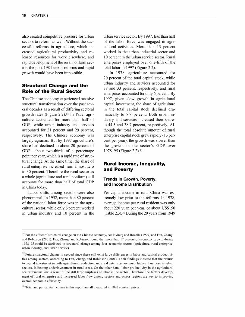
growth rates (Figure 2.2).14 In 1952, agri-
culture accounted for more than half of
GDP, while urban industry and services
accounted for 21 percent and 29 percent,
respectively. The Chinese economy was
largely agrarian. But by 1997 agriculture’s
share had declined to about 20 percent of
GDP—about two-thirds of a percentage
point per year, which is a rapid rate of struc-
tural change. At the same time, the share of
rural enterprise increased from almost zero
to 30 percent. Therefore the rural sector as
a whole (agriculture and rural nonfarm) still
accounts for more than half of total GDP
in China today.
Labor shifts among sectors were also
phenomenal. In 1952, more than 80 percent
of the national labor force was in the agri-
cultural sector, while only 6 percent worked
in urban industry and 10 percent in the
urban service sector. By 1997, less than half
of the labor force was engaged in agri-
cultural activities. More than 13 percent
worked in the urban industrial sector and
10 percent in the urban service sector. Rural
enterprises employed over one-fifth of the
total labor in 1997 (Figure 2.2).
In 1978, agriculture accounted for
20 percent of the total capital stock, while
urban industry and services accounted for
38 and 33 percent, respectively, and rural
enterprises accounted for only 6 percent. By
1997, given slow growth in agricultural
capital investment, the share of agriculture
in the total capital stock declined dra-
matically to 8.8 percent. Both urban in-
dustry and services increased their shares
to 44.5 and 38.7 percent, respectively. Al-
though the total absolute amount of rural
enterprise capital stock grew rapidly (13 per-
cent per year), the growth was slower than
the growth in the sector’s GDP over
1978–95 (Figure 2.2).15
Rural Income, Inequality,and Poverty
Trends in Growth, Poverty,and Income Distribution
Per capita income in rural China was ex-
tremely low prior to the reforms. In 1978,
average income per rural resident was only
about 220 yuan per year, or about US$150
(Table 2.3).16 During the 29 years from 1949
10 CHAPTER 2
14For the effect of structural change on the Chinese economy, see Nyberg and Rozelle (1999) and Fan, Zhang,
and Robinson (2001). Fan, Zhang, and Robinson found that more than 17 percent of economic growth during
1978–95 could be attributed to structural change among four economic sectors (agriculture, rural enterprise,
urban industry, and urban service).
15Future structural change is needed since there still exist large differences in labor and capital productivi-
ties among sectors, according to Fan, Zhang, and Robinson (2001). Their findings indicate that the returns
to capital investment in both agricultural production and rural enterprise are much higher than those in urban
sectors, indicating underinvestment in rural areas. On the other hand, labor productivity in the agricultural
sector remains low, a result of the still large surpluses of labor in the sector. Therefore, the further develop-
ment of rural enterprise and increased labor flow among sectors and across regions are key to improving
overall economic efficiency.
16Total and per capita incomes in this report are all measured in 1990 constant prices.
to 1978, per capita income increased by
only 95 percent, or 2.3 percent per annum.
China was one of the poorest countries in
the world. Most rural people struggled to
survive from day to day. In 1978, 260 mil-
lion residents in rural China, or 33 percent
of the total rural population, lived below the
poverty line, without access to sufficient
food or income to maintain a healthy and
productive life.
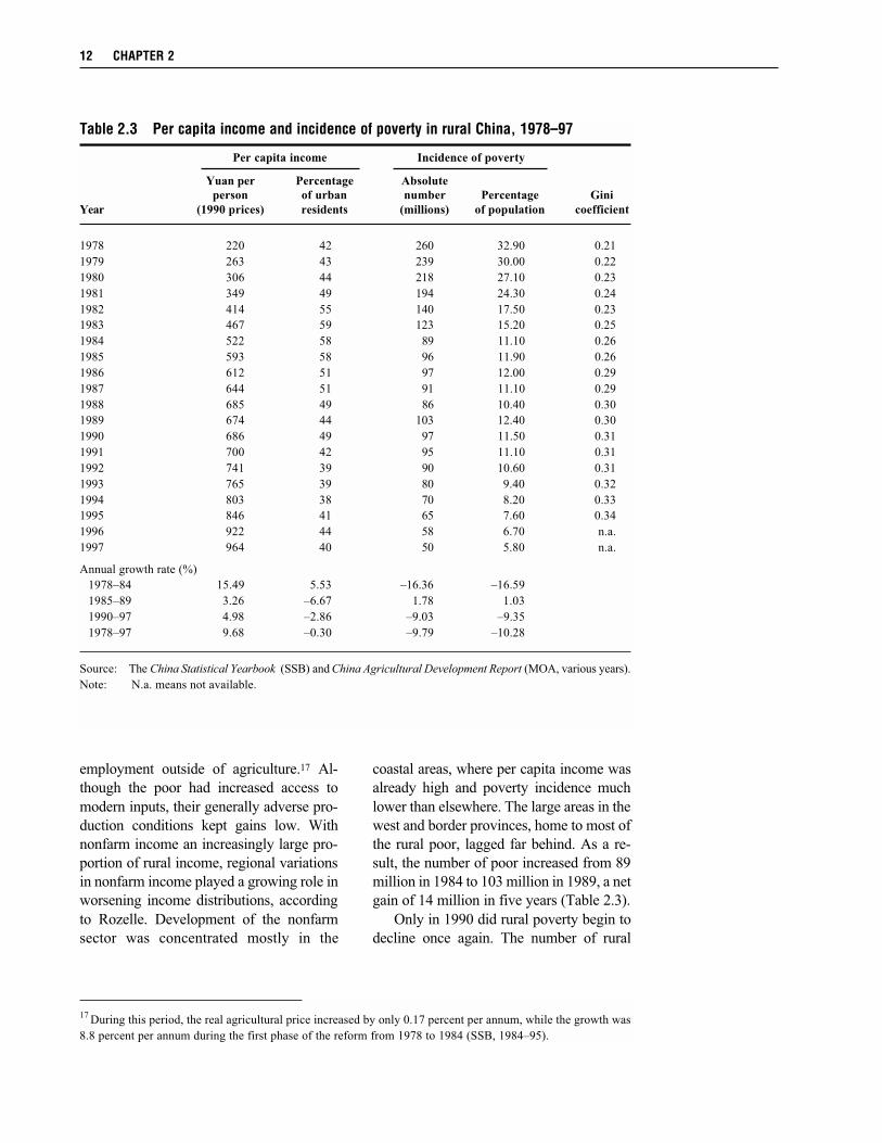
This changed dramatically directly
after the initiation of rural reforms in 1978.
Per capita income increased to 522 yuan
in 1984 from 220 yuan in 1978, a growth
rate of 15 percent per annum (Table 2.3).
The income gains were shared widely
enough to cut the number of poor, hence
the rate of poverty, by more than half By
1984, only 11 percent of the rural popu-
lation was below the poverty line. Be-
cause of the equitable distribution of
land to families, income inequality,
measured as Gini coefficient, increased
only slightly (Figure 2.3).
During the second stage of reforms
(1985–89), rural income continued to in-
crease, but at the much slower pace of
3 percent per annum (Table 2.3). This was
due mainly to the stagnation of agricul-
tural production after the reforms, as dis-
cussed in the previous section. The effects
of fast agricultural growth on rural pov-
erty were largely exhausted by the end
of 1984. Over this same period, rural in-
come distribution became less egalitarian,
and the Gini index rose from 0.264 to
0.301 (SSB 1990). The ratio of per capita
rural income in coastal regions to that
in other areas also increased, from 1.21
to 1.51 (Zhang and Kanbur 2001). The
changes in income distribution probably
resulted from the changed nature of in-
come gains and the growing differential
in rural nonfarm opportunities among re-
gions (Rozelle 1994).
With real crop prices stagnating and
input prices rising, rural income gains had
to come from increased efficiency in agri-
cultural production and marketing or from
GROWTH, INEQUALITY, AND POVERTY 11
Figure 2.2 Structural shift of GDP, labor, and capital, 1978–97
Source: Fan, Zhang, and Robinson 2001.
Note: Total capital stock data only go up to 1995.
employment outside of agriculture.17 Al-
though the poor had increased access to
modern inputs, their generally adverse pro-
duction conditions kept gains low. With
nonfarm income an increasingly large pro-
portion of rural income, regional variations
in nonfarm income played a growing role in
worsening income distributions, according
to Rozelle. Development of the nonfarm
sector was concentrated mostly in the
coastal areas, where per capita income was
already high and poverty incidence much
lower than elsewhere. The large areas in the
west and border provinces, home to most of
the rural poor, lagged far behind. As a re-
sult, the number of poor increased from 89
million in 1984 to 103 million in 1989, a net
gain of 14 million in five years (Table 2.3).
Only in 1990 did rural poverty begin to
decline once again. The number of rural
12 CHAPTER 2
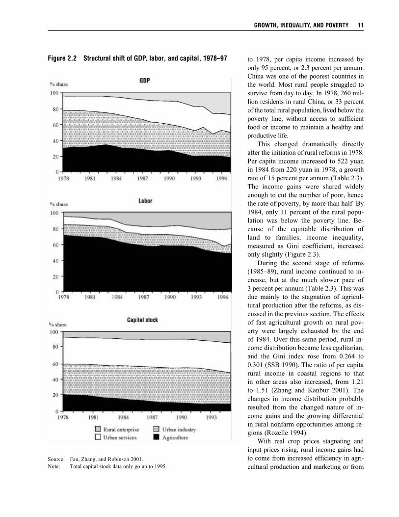
Table 2.3 Per capita income and incidence of poverty in rural China, 1978–97
Per capita income Incidence of poverty
Yuan per Percentage Absolute
person of urban number Percentage Gini
Year (1990 prices) residents (millions) of population coefficient
1978 220 42 260 32.90 0.21
1979 263 43 239 30.00 0.22
1980 306 44 218 27.10 0.23
1981 349 49 194 24.30 0.24
1982 414 55 140 17.50 0.23
1983 467 59 123 15.20 0.25
1984 522 58 89 11.10 0.26
1985 593 58 96 11.90 0.26
1986 612 51 97 12.00 0.29
1987 644 51 91 11.10 0.29
1988 685 49 86 10.40 0.30
1989 674 44 103 12.40 0.30
1990 686 49 97 11.50 0.31
1991 700 42 95 11.10 0.31
1992 741 39 90 10.60 0.31
1993 765 39 80 9.40 0.32
1994 803 38 70 8.20 0.33
1995 846 41 65 7.60 0.34
1996 922 44 58 6.70 n.a.
1997 964 40 50 5.80 n.a.
Annual growth rate (%)
1978–84 15.49 5.53 –16.36 –16.59
1985–89 3.26 –6.67 1.78 1.03
1990–97 4.98 –2.86 –9.03 –9.35
1978–97 9.68 –0.30 –9.79 –10.28
Source: The China Statistical Yearbook (SSB) and China Agricultural Development Report (MOA, various years).
Note: N.a. means not available.
17During this period, the real agricultural price increased by only 0.17 percent per annum, while the growth was
8.8 percent per annum during the first phase of the reform from 1978 to 1984 (SSB, 1984–95).
poor dropped 9 percent per annum, from
103 million in 1989 to 50 million in 1997.
Moreover, the rate of rural poverty reduc-
tion was faster than that of income growth
(5 percent per annum) during the period, in-
dicating that factors other than income
growth were at play. In 1995, the govern-
ment set itself a target of eliminating all
rural poverty by 2000. To accomplish that
goal, it introduced a series of policies and
committed substantial financial resources.
Rural residents earned less than half
their urban cohorts in 1978, with rural in-
come 42 percent of that in urban areas
(Table 2.3). Due to the success of rural re-
forms, that percentage increased to 59 per-
cent in 1983. But it declined again to
40 percent in 1997, mainly owing to fast
growth in urban areas and relatively slug-
gish increases in rural earnings.
Poverty in China is therefore still
mainly a rural phenomenon. Urban poor
have been relatively few in number in
China, although income distribution in the
cities has deteriorated in recent years (Park,
Wang, and Wu 2001; World Bank 1992). In
1990, average per capita income among the
poorest 5 percent of urban residents was
689 yuan, more than double the urban ab-
solute poverty line of 321 yuan and greater
than the per capita income of 65 percent of
rural residents. Less than 1 percent of the
urban population—about one million peo-
ple—had incomes below the estimated ab-
solute poverty line each year from 1983 to
1990. Higher income levels, complemented
by annual consumer food subsidies of at
least 200 yuan per urban recipient, left the
registered urban population much better
nourished than their rural counterparts. In
more recent years, however, many former
state employees were laid off due to the re-
form of state-owned enterprises. Incidence
of urban poverty may therefore have in-
creased. Nevertheless, the size and severity
of urban poverty remains of a much lesser
scale than in the rural areas.
GROWTH, INEQUALITY, AND POVERTY 13
Figure 2.3 Income, inequality, and change in poverty in ruralChina, 1978–97
Source: Table 2.3.
Note: Gini coefficient estimates only go up to 1995.
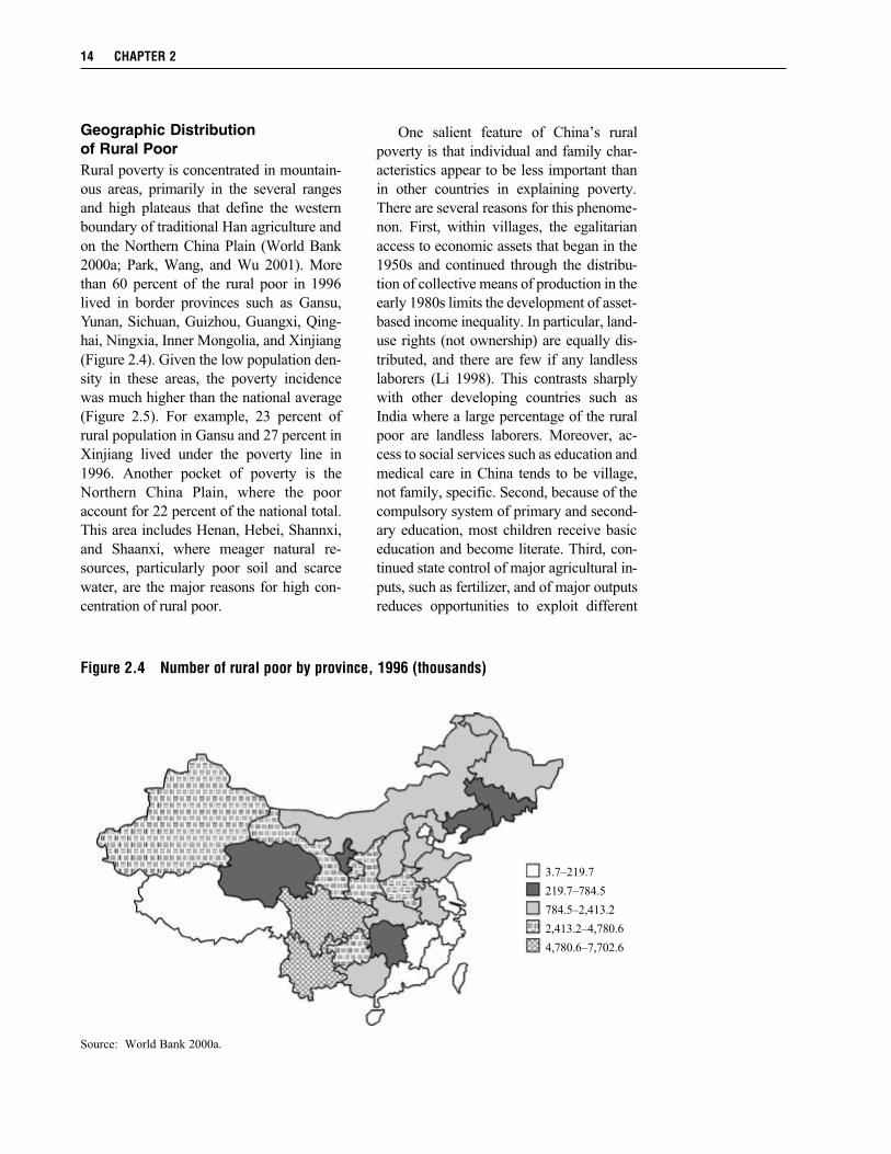
Geographic Distributionof Rural PoorRural poverty is concentrated in mountain-
ous areas, primarily in the several ranges
and high plateaus that define the western
boundary of traditional Han agriculture and
on the Northern China Plain (World Bank
2000a; Park, Wang, and Wu 2001). More
than 60 percent of the rural poor in 1996
lived in border provinces such as Gansu,
Yunan, Sichuan, Guizhou, Guangxi, Qing-
hai, Ningxia, Inner Mongolia, and Xinjiang
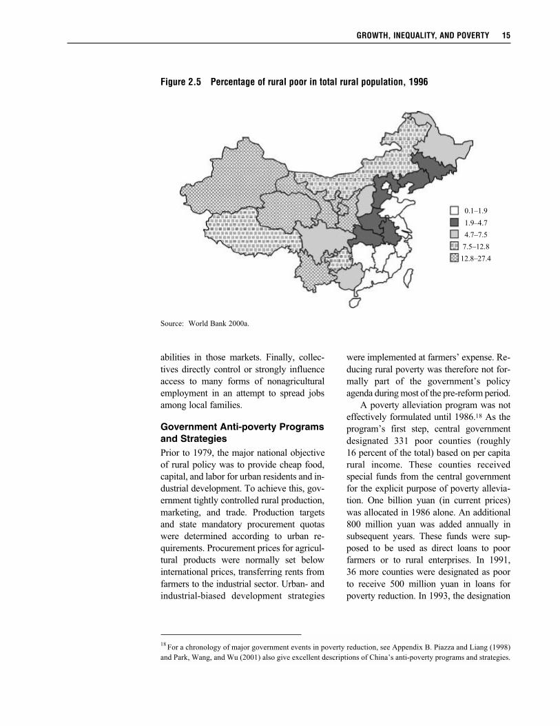
(Figure 2.4). Given the low population den-
sity in these areas, the poverty incidence
was much higher than the national average
(Figure 2.5). For example, 23 percent of
rural population in Gansu and 27 percent in
Xinjiang lived under the poverty line in
1996. Another pocket of poverty is the
Northern China Plain, where the poor
account for 22 percent of the national total.
This area includes Henan, Hebei, Shannxi,
and Shaanxi, where meager natural re-
sources, particularly poor soil and scarce
water, are the major reasons for high con-
centration of rural poor.
One salient feature of China’s rural
poverty is that individual and family char-
acteristics appear to be less important than
in other countries in explaining poverty.
There are several reasons for this phenome-
non. First, within villages, the egalitarian
access to economic assets that began in the
1950s and continued through the distribu-
tion of collective means of production in the
early 1980s limits the development of asset-
based income inequality. In particular, land-
use rights (not ownership) are equally dis-
tributed, and there are few if any landless
laborers (Li 1998). This contrasts sharply
with other developing countries such as
India where a large percentage of the rural
poor are landless laborers. Moreover, ac-
cess to social services such as education and
medical care in China tends to be village,
not family, specific. Second, because of the
compulsory system of primary and second-
ary education, most children receive basic
education and become literate. Third, con-
tinued state control of major agricultural in-
puts, such as fertilizer, and of major outputs
reduces opportunities to exploit different
14 CHAPTER 2
Figure 2.4 Number of rural poor by province, 1996 (thousands)
Source: World Bank 2000a.
3.7–219.7
219.7–784.5
784.5–2,413.2
2,413.2–4,780.6
4,780.6–7,702.6
abilities in those markets. Finally, collec-
tives directly control or strongly influence
access to many forms of nonagricultural
employment in an attempt to spread jobs
among local families.
Government Anti-poverty Programsand StrategiesPrior to 1979, the major national objective
of rural policy was to provide cheap food,
capital, and labor for urban residents and in-
dustrial development. To achieve this, gov-
ernment tightly controlled rural production,
marketing, and trade. Production targets
and state mandatory procurement quotas
were determined according to urban re-
quirements. Procurement prices for agricul-
tural products were normally set below
international prices, transferring rents from
farmers to the industrial sector. Urban- and
industrial-biased development strategies
were implemented at farmers’ expense. Re-
ducing rural poverty was therefore not for-
mally part of the government’s policy
agenda during most of the pre-reform period.
A poverty alleviation program was not
effectively formulated until 1986.18 As the
program’s first step, central government
designated 331 poor counties (roughly
16 percent of the total) based on per capita
rural income. These counties received
special funds from the central government
for the explicit purpose of poverty allevia-
tion. One billion yuan (in current prices)
was allocated in 1986 alone. An additional
800 million yuan was added annually in
subsequent years. These funds were sup-
posed to be used as direct loans to poor
farmers or to rural enterprises. In 1991,
36 more counties were designated as poor
to receive 500 million yuan in loans for
poverty reduction. In 1993, the designation
GROWTH, INEQUALITY, AND POVERTY 15
Figure 2.5 Percentage of rural poor in total rural population, 1996
18For a chronology of major government events in poverty reduction, see Appendix B. Piazza and Liang (1998)
and Park, Wang, and Wu (2001) also give excellent descriptions of China’s anti-poverty programs and strategies.
Source: World Bank 2000a.
0.1–1.9
1.9–4.7
4.7–7.5
7.5–12.8
12.8–27.4
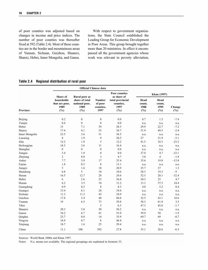
of poor counties was adjusted based on
changes in income and price indices. The
number of poor counties was thereafter
fixed at 592 (Table 2.4). Most of these coun-
ties are in the border and mountainous areas
of Yunnan, Sichuan, Guizhou, Shaanxi,
Shanxi, Hebei, Inner Mongolia, and Gansu.
With respect to government organiza-
tions, the State Council established the
Leading Group for Economic Development
in Poor Areas. This group brought together
more than 20 ministries. In effect it encom-
passed all the government agencies whose
work was relevant to poverty alleviation,
16 CHAPTER 2
Table 2.4 Regional distribution of rural poor
Official Chinese data
Khan (1997)Poor counties
Share of Rural poor as as share of
households share of total Number total provincial Head Head
that are poor, national poor, of poor counties, count, count,
1989 1989 counties, 1997 1988 1995 Change
Province (%) (%) 1997 (%) (%) (%) (%)
Beijing 0.2 0 0 0.0 8.7 1.3 –7.4
Tianjin 0.4 0 0 0.0 n.a. n.a. n.a.
Hebei 13 7.1 39 28.3 29.9 22.7 –7.2
Shanxi 17.4 4.1 35 34.7 51.9 49.5 –2.4
Inner Mongolia 23.5 3.6 31 36.5 n.a. n.a. n.a.
Liaoning 8 1.9 9 20.5 27 21.9 –5.1
Jilin 12.2 1.9 5 12.2 41.5 18.3 –23.2
Heilongjian 18.3 3.6 11 16.4 n.a. n.a. n.a.
Shanghai 0 0 0 0.0 n.a. n.a. n.a.
Jiangsu 3.4 1.9 0 0.0 27.8 4.7 –23.1
Zhejiang 2 0.8 3 4.7 5.8 4 –1.8
Anhui 7.7 3.9 17 25.4 35.6 19.8 –15.8
Fujian 1.8 0.5 8 13.1 n.a. n.a. n.a.
Jiangxi 5 1.6 18 20.9 25.7 27 1.3
Shandong 6.8 5 10 10.6 28.3 19.3 –9
Henan 16.5 12.7 28 24.6 52.5 20.1 –32.4
Hubei 6 2.6 25 36.8 20.3 25 4.7
Hunan 6.2 3.5 10 11.2 13.1 37.5 24.4
Guangdong 0.9 0.5 8 8.3 4.8 5.2 0.4
Guangxi 15.4 6.1 28 34.6 n.a. n.a. n.a.
Sichuan 11.2 11.2 43 24.9 n.a. n.a. n.a.
Guizhou 17.8 5.4 48 60.8 32.5 43.1 10.6
Yunnan 19 6.5 73 59.8 58.3 61.8 3.5
Tibet 5 6.5 47.3 45.6 –1.7
Shaanxi 20.3 5.8 50 56.2 n.a. n.a. n.a.
Gansu 34.2 6.7 41 53.9 59.9 58 –1.9
Qinghai 23.7 0.8 14 35.9 69.7 69 –0.7
Ningxia 18.9 0.7 8 44.4 n.a. n.a. n.a.
Xinjiang 18.7 1.6 25 29.4 n.a. n.a. n.a.
China 11.1 100 592 27.8 35.1 28.6 –6.5
Sources: World Bank 2000a and Khan 1997.
Notes: N.a. means not available. The regional groupings are explained in footnote 33.
thus providing a mechanism both to influ-
ence the initiatives taken by the various min-
istries and to seek coordination in this area.
China’s poverty alleviation strategy
developed in three steps. Prior to 1984, so-
cial welfare and relief funds were mainly
used to subsidize poor families. No formal
strategy existed for reducing the number of
poor in rural areas. From 1984 to 1995,
government pursued a strategy of “regional
targeting,” that is, alleviating poverty by de-
veloping regional or local economies. This
strategy effectively wiped out large-scale
poverty by developing poor areas, although
it brought little benefit to the extremely
poor in the poorest areas. The poor were
thus increasingly concentrated in remote
locales with limited access to roads and
other infrastructure, making it difficult for
the development of the regional economy to
trickle down to them. After 1996, the gov-
ernment altered its strategy to one of target-
ing poor households directly.
One program under this strategy is the
food-for-work program, designed to build
necessary infrastructure in poor rural areas.
The scheme provides a fund through which
roads, irrigation, and other construction
projects are carried out by extremely poor
farmers, most of whom are identified by
village heads. Those employed on the proj-
ects sometimes receive food or, more fre-
quently, vouchers that can be exchanged for
food and other basic necessities.19
GROWTH, INEQUALITY, AND POVERTY 17
19 Several studies assess the effects of these programs (Zhu and Jiang 1995; Park, Wang, and Wu 2001),
concluding that most are modestly effective in rural poverty reduction.
C H A P T E R 3
Public Capital and Investment
T his chapter reviews the development of technology, education, and infrastructure and
government spending on these types of capital. Such investments are a major source of
long-term economic growth and poverty reduction. They have contributed not only to
growth in agricultural production, providing an adequate food supply for the ever larger and
richer population, but also to development of the rural nonfarm sector. The latter has become
increasingly important for further poverty reduction in rural areas.
Research
China’s agricultural research system expanded rapidly during the past four decades to become
one of the largest public systems in the world. It employed more than 50,000 senior scientists
and spent 4.1 billion current yuan (or 2.2 billion yuan in 1990 prices) on research conducted
in national, provincial, and prefecture research institutes and agricultural universities in
1997.20 By the early 1990s, the latest years for which comparative figures are available, the
Chinese system accounted for over 18 percent of the less developed world’s agricultural re-
search expenditures (Pardey, Roseboom, and Fan 1998).
Nonetheless, the Chinese agricultural research system experienced many ups and downs
over the last several decades. China’s investment in agricultural research was minimal right
after the founding of the People’s Republic in 1949, but it grew rapidly thereafter until 1960.
Growth in the 1960s was relatively slow due to the Great Famine (1959–61) and the Cultural
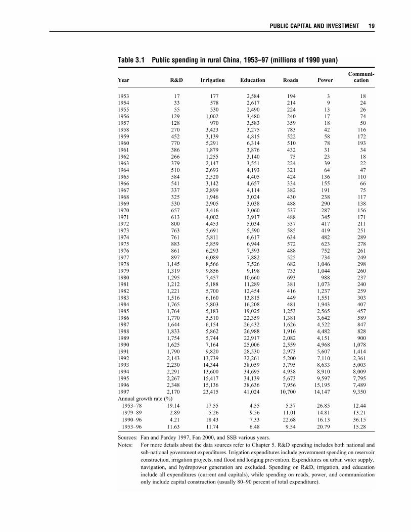
Revolution (1966–76). Although investment increased steadily during the 1970s (Table 3.1),
growth slowed in the 1980s to 23 percent during the entire 10 year period. In the 1990s, agri-
cultural research expenditures again began to rise, largely due to government efforts to boost
grain production through science and technology.
As a percentage of agricultural gross domestic product (AgGDP), agricultural research
investment was relatively low during the first five-year plan period, at 0.12 percent, but it
increased to 0.56 percent for the period 1958–76. The percentage then gradually declined to
0.3 percent in recent years. However, since AgGDP has grown rapidly, government invest-
ment in agricultural research has increased substantially in absolute terms over the last several
decades, but it declined relative to the size of the agricultural sector (Fan 2000). In compari-
son with other low-income countries in Asia, China moved from investing relatively more
20In 1997, research expenditures in the Chinese agricultural research system (including research expenses by
agricultural universities) were 4.1 billion in current Chinese yuan. This is equivalent to US$500 million meas-
ured by nominal exchange rate, and $2.03 billion measured by 1997 purchasing power parity.
18
PUBLIC CAPITAL AND INVESTMENT 19
Table 3.1 Public spending in rural China, 1953–97 (millions of 1990 yuan)
Communi-Year R&D Irrigation Education Roads Power cation
1953 17 177 2,584 194 3 18
1954 33 578 2,617 214 9 24
1955 55 530 2,490 224 13 26
1956 129 1,002 3,480 240 17 74
1957 128 970 3,583 359 18 50
1958 270 3,423 3,275 783 42 116
1959 452 3,139 4,815 522 58 172
1960 770 5,291 6,314 510 78 193
1961 386 1,879 3,876 432 31 34
1962 266 1,255 3,140 75 23 18
1963 379 2,147 3,551 224 39 22
1964 510 2,693 4,193 321 64 47
1965 584 2,520 4,405 424 136 110
1966 541 3,142 4,657 334 155 66
1967 337 2,899 4,114 382 191 75
1968 325 1,946 3,024 430 238 117
1969 530 2,905 3,038 488 290 138
1970 657 3,416 3,060 537 287 156
1971 613 4,002 3,917 488 345 171
1972 800 4,453 5,034 537 417 211
1973 763 5,691 5,590 585 419 251
1974 761 5,811 6,617 634 482 289
1975 883 5,859 6,944 572 623 278
1976 861 6,293 7,593 488 752 261
1977 897 6,089 7,882 525 734 249
1978 1,145 8,566 7,526 682 1,046 298
1979 1,319 9,856 9,198 733 1,044 260
1980 1,295 7,457 10,660 693 988 237
1981 1,212 5,188 11,289 381 1,073 240
1982 1,221 5,700 12,454 416 1,237 259
1983 1,516 6,160 13,815 449 1,551 303
1984 1,765 5,803 16,208 481 1,943 407
1985 1,764 5,183 19,025 1,253 2,565 457
1986 1,770 5,510 22,359 1,381 3,642 589
1987 1,644 6,154 26,432 1,626 4,522 847
1988 1,833 5,862 26,988 1,916 4,482 828
1989 1,754 5,744 22,917 2,082 4,151 900
1990 1,625 7,164 25,006 2,559 4,968 1,078
1991 1,790 9,820 28,530 2,973 5,607 1,414
1992 2,143 13,739 32,261 5,200 7,110 2,361
1993 2,230 14,344 38,059 3,795 8,633 5,003
1994 2,291 13,600 34,695 4,938 8,910 8,009
1995 2,267 15,417 34,139 5,673 9,597 7,795
1996 2,348 15,136 38,636 7,956 15,195 7,489
1997 2,170 23,415 41,024 10,700 14,147 9,350
Annual growth rate (%)
1953–78 19.14 17.55 4.55 5.37 26.85 12.44
1979–89 2.89 –5.26 9.56 11.01 14.81 13.21
1990–96 4.21 18.43 7.33 22.68 16.13 36.15
1953–96 11.63 11.74 6.48 9.54 20.79 15.28
Sources: Fan and Pardey 1997, Fan 2000, and SSB various years.
Notes: For more details about the data sources refer to Chapter 5. R&D spending includes both national and
sub-national government expenditures. Irrigation expenditures include government spending on reservoir
construction, irrigation projects, and flood and lodging prevention. Expenditures on urban water supply,
navigation, and hydropower generation are excluded. Spending on R&D, irrigation, and education
include all expenditures (current and capitals), while spending on roads, power, and communication
only include capital construction (usually 80–90 percent of total expenditure).
20 CHAPTER 3
than average during the 1970s to below
average at present (Pardey, Roseboom, and
Fan 1998).
Agricultural research expenditure as a
percentage of total government spending
was comparatively low in the 1950s, aver-
aging 0.10 percent during 1953–57 and
0.38 percent for 1958–60. Thereafter, the
ratios of government spending remained
relatively stable, hovering around 0.50 to
0.55 percent except during the Cultural
Revolution when the share was substan-
tially lower. Agricultural research spending
as a share of total national research and de-
velopment (R&D) expenditures was also
quite stable. China earmarked some 10 to
13 percent of total R&D expenditures for
agriculture during the past four decades. In
contrast, agricultural research expenditures
as a percentage of government spending
on agriculture increased steadily, from just
1.5 percent during the first five-year plan
period to surpass 6 percent in the last decade.
The development of China’s research
personnel has not matched the pattern of
funds allocated to research. Specifically,
three phases can be identified. During the
1950s and 1960s the number of researchers
increased steadily. By 1973 about 10,000
scientists worked in the Chinese system.21
From 1973 to 1990, numbers of research
personnel increased rapidly, to almost
60,000 researchers, a rate of increase in
excess of 10 percent per annum. During
the third stage (after 1990), the number of
researchers stabilized at around 60,000.
After 1995, the number of researchers de-
clined marginally, to about 53,000 in 1997.
Increased numbers of researchers from
new graduates combined with a lack of
growth in expenditures caused expenditure
per scientist to drop sharply from 1979 to
1991. Although in more recent years ex-
penditure per scientist has increased sub-
stantially in nominal terms, in real terms it
has grown only marginally.
The regional pattern of R&D expendi-
tures reveals that the Northwest region (Gan-
su, Shaanxi, Qinghai, Ningxia, and Xin-
jiang) spent much less than coastal areas,
and expenditures of the latter were stagnant
or even declining in the 1990s (Table C.2).
It is not surprising that land productivity in
the Northwest region was lowest among all
regions. The coastal provinces (Guang-
dong, Zhejiang, Jiangsu, and Shangdong)
experienced the most rapid growth in agri-
culture R&D spending.
Several studies have attempted to quan-
tify the effects and returns of research in-
vestment on agricultural production. Fan
and Pardey (1997) attributed about 20 per-
cent of agricultural output growth from
1965 to 1993 to increased public invest-
ment in agricultural R&D. Rates of return
to investment estimated using different lag
structures range from 36 percent to 90 per-
cent in 1997 (Fan 2000). Huang, Rozelle,
and Rosegrant (1999) suggest that if China
increased its investment in agricultural re-
search and irrigation by 4.5 percent per
year, it could become a net exporter of
grains by 2020. With every 1 percent in-
crease in agricultural research and irrigation
investment, China could produce an addi-
tional 21 million metric tons of grain in
2010 and 36 million metric tons in 2020.
Increased agricultural production from re-
search investments has undoubtedly trick-
led down to the rural poor, although few
studies have quantified their effect on
poverty reduction.
Irrigation
Because rainfall is concentrated during the
monsoon, China’s early civilizations devel-
oped an agricultural system that depended
21 Research personnel here are defined as researchers who have at least a bachelor’s degree and one to two years
of research experience. They are commonly referred to as scientists and engineers in the Chinese system.
PUBLIC CAPITAL AND INVESTMENT 21
on water conservation and irrigation. The
Dujiang Weir in Sichuan Province, dating
from the third century B.C., still supplies
water to 200, 000 hectares. During the Ming
and Qing dynasties, extensive irrigation
works were developed in the north and cen-
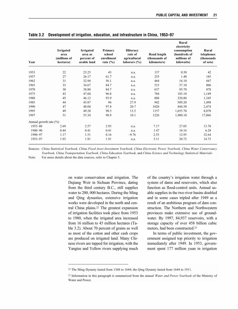
tral China plains.22 The greatest expansion
of irrigation facilities took place from 1953
to 1980, when the irrigated area increased
from 16 million to 45 million hectares (Ta-
ble 3.2). About 70 percent of grains as well
as most of the cotton and other cash crops
are produced on irrigated land. Many Chi-
nese rivers are tapped for irrigation, with the
Yangtze and Yellow rivers supplying much
of the country’s irrigation water through a
system of dams and reservoirs, which also
function as flood-control units. Annual us-
able supplies in the two river basins doubled
and in some cases tripled after 1949 as a
result of an ambitious program of dam con-
struction. The Northern and Northwestern
provinces make extensive use of ground-
water. By 1997, 84,937 reservoirs, with a
storage capacity of over 458 billion cubic
meters, had been constructed.23
In terms of public investment, the gov-
ernment assigned top priority to irrigation
immediately after 1949. In 1953, govern-
ment spent 177 million yuan in irrigation
22 The Ming Dynasty lasted from 1368 to 1644; the Qing Dynasty lasted from 1644 to 1911.
23 Information in this paragraph is summarized from the annual Water and Power Yearbook of the Ministry of
Water and Power.
Table 3.2 Development of irrigation, education, and infrastructure in China, 1953–97
Rural
electricity
Irrigated Irrigated Primary Illiteracy consumption Rural
area area as school rate of Road length (hundreds of telephones
(millions of percent of enrollment agricultural (thousands of millions of (thousands
Year hectares) arable land rate (%) laborers (%) kilometers) kilowatts) of sets)
1953 22 23.25 43 n.a. 137 0.50 42
1957 27 26.17 61.7 n.a. 255 1.40 185
1962 31 32.94 56.1 n.a. 464 16.10 847
1965 33 34.67 84.7 n.a. 515 37.10 806
1970 38 38.80 84.7 n.a. 637 95.70 878
1975 43 47.60 96.8 n.a. 784 183.10 1,149
1980 45 46.12 93.9 n.a. 888 320.80 1,345
1985 44 45.87 96 27.9 942 509.20 1,498
1990 47 48.04 97.8 20.7 1028 844.50 2,474
1995 49 49.28 98.5 13.5 1157 1,655.70 8,070
1997 51 53.34 98.9 10.1 1226 1,980.10 17,866
Annual growth rate (%)
1953–80 2.69 2.57 2.93 n.a. 7.17 27.05 13.70
1980–90 0.44 0.41 0.41 n.a. 1.47 10.16 6.28
1990–97 1.17 1.51 0.16 –9.76 2.55 12.95 32.64
1953–97 1.93 1.91 1.91 n.a. 5.11 20.72 14.75
Sources: China Statistical Yearbook, China Fixed Asset Investment Yearbook, China Electronic Power Yearbook, China Water Conservancy
Yearbook, China Transportation Yearbook, China Education Yearbook, and China Science and Technology Statistical Materials.
Note: For more details about the data sources, refer to Chapter 5.
investment, 10 times more than investment
in agricultural research.24 The investment in
irrigation continued to increase until 1966.
Under the commune system, it was rather
easy for government to mobilize large num-
bers of rural laborers to work on the proj-
ects. As a result of this increased invest-
ment, more than 10 million hectares of land
were brought under irrigation (Table 3.2).
However, the investment increased very lit-
tle from 1976 to 1990. In fact, it declined
over 1976–89 (Table 3.1). During this pe-
riod, there was no increase in irrigated areas
in Chinese agricultural production.
In response to the grain shortfall and
large imports in 1994–95, the government
increased its investment in irrigation
markedly in 1996 and 1997. Among all re-
gions, the Northwest accounted for the
largest increase in the 1990s, followed by
the Northern China Plain (Table C.2). In-
vestments in the Northeast and Southwest
remained flat during most of the 1990s. De-
spite the increased spending, irrigated areas
as a percentage of total land area increased
very little. The only exception was the
Northern China Plain (Table C.6). Further
expansion of irrigated areas has proved dif-
ficult because of competing industrial and
residential uses of water resources. As a re-
sult, returns to irrigation investment may
decline in the future.
Education
The root of formal education in China dates
back to at least the Shang Dynasty of
1523–1027 B.C. Up until the end of the
Qing Dynasty of 1644–1911, education was
limited to a privileged few, mostly for pro-
ducing government officials.
Shortly after the the Chinese Commu-
nists took power, a Soviet-type educational
system was imported with little concern
about the special features of the Chinese
environment. At the time, the Soviet Union
was regarded as the new prototype for suc-
cess. But the Soviet model was largely
driven by technological needs; it paid little
attention to the problem of mass illiteracy
that China faced. By 1956, less than half of
primary- and secondary-aged children were
in school. Most efforts during this period
were devoted to developing and restructur-
ing higher education. As a result of this re-
structuring, the number of comprehensive
universities diminished while the number of
specialized colleges increased significantly.
The periods of the Great Leap Forward
(1958–60) and the subsequent Cultural
Revolution (1966–76) were disruptive
times for Chinese society in general and its
education in particular. Educational infra-
structure was decimated as a result of the
revolutionary struggles, and students suf-
fered vastly watered-down or nonexistent
curricula. Perhaps the only gain (again at
the expense of quality) was the delivery of
elementary education to an unprecedented
number of school-aged children, largely be-
cause agricultural collectivization enabled
the creation of large numbers of “commune
schools.” These were overseen directly by
the collectives rather than by higher-level
agencies. The enrollment rate of school-
aged children rose from 43 percent to 97 per-
cent by 1976 (Table 3.2). In 1983 more than
90 percent of rural children were enrolled in
school, only slightly less than the urban rate
of 98 percent (SSB, 1980–2000).
After 1978, China adopted the “nine-
year compulsory schooling” education
policy. That meant all children were re-
quired to attend school for at least nine
years to finish both primary and junior
middle school.
22 CHAPTER 3
24 Irrigation investments here include only those directly related to irrigation, such as reservoir construction,
irrigation projects, and flood and lodging prevention. The investments in total water conservancy, which also
includes urban water supply and hydropower generation, amounted to more than 1 billion yuan in 1953, 60 times
higher than agricultural R&D investment.
As a result of these efforts, the illiteracy
rate of the general population 15 years and
older dropped from 48 percent in 1970 to
less than 10 percent in 1997. In particular,
illiteracy among agricultural laborers de-
clined from 28 percent in 1985 to 10 per-
cent in 1997 (Table 3.2). Consequently,
labor quality improved substantially. This
enhanced human capital in rural areas and
provided great opportunities for farmers to
use modern farming technology and to en-
gage in nonfarm activities both in rural
township and village enterprises and in
urban industrial centers.
T. Paul Schultz (1987) has shown that
increased government efforts in rural pri-
mary education not only have large eco-
nomic returns, but also contribute to equity
in rural areas. Although the high returns to
education in rural China were not systemat-
ically documented, anecdotal evidence sug-
gests that improved education (particularly
of household heads) not only enhanced
farm productivity (Nguyen and Cheng
1997; Li and Zhang 1998), but also im-
proved farmers’ off-farm opportunities and
their ability to migrate to urban sectors
(Zhao 1999; Yang 1997).
In terms of expenditure, China spent
about 2 percent of national gross domestic
product (GDP) on education, which is
much lower than many developed countries
but higher than most developing countries.
However, total expenditure on education
may in fact be much higher because rural
education is also largely supported by rural
communities, and their investment is not
counted in the formal government budget.
Despite extraordinary success in basic
education in China, many poor were not
reached by the government efforts. Official
provincial-level data presented in Table C.3
reveals astonishing differences among
provinces in illiteracy rates of rural labor-
ers. Not only was illiteracy higher in the
western region, but its rate of decline there
was the lowest of all provinces. The dispar-
ity can be even greater within a single
province or county. According to official
statistics, in the poorer half of the townships
of 35 counties supported by a World Bank
project in Yunnan, Guizhou, and Guangxi,
average enrollment was at least 10 percent-
age points lower than the national average
for the same age group (Piazza and Liang
1998). Special household surveys docu-
ment even greater disparities at the village
level. The State Statistical Bureau’s (SSB)
1994 survey of 600 households in the poor-
est townships of these 35 counties showed
that the average enrollment rate for children
ages 6–12 was only 55 percent. It is there-
fore unsurprising that official statistics in
these counties indicate an average literacy
rate for the total population of only 35 per-
cent according to Piazza and Liang.
Infrastructure
Development of rural infrastructure is key
to rural social and economic life. But until
recently, China’s government gave rela-
tively low priority to rural infrastructure in
promoting agricultural production, rural
nonfarm employment, and improved living
standards for the rural population.
Among all transportation facilities,
roads are the most crucial to rural develop-
ment. However, the mountainous topog-
raphy in many parts of China has hindered
the development of roads. In 1953, total
length of roads was only about 137,000 kil-
meters (Table 3.2), and road density was
about 14 kilometers per thousand square
kilometers, much lower than that of India
at the time.25 Moreover, government invest-
ment in road construction increased very
little from 1953 to 1976. Nevertheless, the
length of roads has increased gradually.
After 1985, the government geared up its
PUBLIC CAPITAL AND INVESTMENT 23
25India’s road density was 129 kilometers per thousand square kilometers in 1950.
investment in roads, particularly high-quality
roads such as highways connecting major
industrial centers in coastal areas. Rural
roads, usually of lower quality, accounted
for about 70 percent of total road length.
In contrast to road development, one of
the greatest achievements in rural China
was the rapid electrification of rural areas
during the past several decades. Introduc-
tion of electricity can profoundly affect vil-
lage life. Electric lighting expands the pro-
ductive and social hours in the day. Radios
and television provide accessible, afford-
able entertainment and education. Power
machinery can raise productivity and im-
prove working conditions.
In the past several decades, China gave
higher priority to electricity than to road
development in its investment portfolio.
Investment in power increased ninetyfold.
Electricity consumption in rural areas
increased from almost zero in 1950 to
198 billion kilowatts in 1997 (Table 3.2).
The most rapid growth occurred in the
1970s and 1980s. The percentage of vil-
lages with access to electricity was 97 per-
cent in 1996, and more than 95 percent of
households had an electrical connection
(Ministry of Electric Power 1997). This
percentage was much higher than that of
India in the same year.
Prior to 1980, growth in government in-
vestment in rural telecommunications was
very slow. Investment increased from 3 mil-
lion yuan in 1953 to 237 million yuan in
1980. However, large-scale development
happened only in recent years, with the
number of rural telephones increasing from
3.4 million in 1992 to 17.9 million in 1997
(Table 3.2). This was largely a result of both
public and private investments in the sector.
From 1989 to 1997, public investment alone
increased more than tenfold.
But this trend at the national level
disguises large regional differences in
rural telecommunications development. As
Table C.5 shows, the coastal provinces like
Guangdong, Jiangsu, Zhejiang, and Fujinag
experienced an exponential growth in the
number of rural telephone sets, while west-
ern regions (Northwest and Southwest)
showed relatively slow growth.
24 CHAPTER 3
C H A P T E R 4
Conceptual Framework and Model
T his chapter reviews previous studies and develops a conceptual framework for the
analysis. It then constructs and specifies the equations system based on previous
studies, a theoretical economic framework, and reality in rural China.
Previous Studies
This section looks at the relevant studies on growth, regional inequality, and poverty reduction
in rural China. In particular, it points out the knowledge gap in previous studies and develops
the rationale for the current study.
Sources of GrowthThe outstanding performance of Chinese agriculture after the reforms of the late 1970s trig-
gered numerous studies to analyze the sources of the rapid growth. These include McMillan,
Whalley, and Zhu (1989); Fan (1991); Lin (1992); Zhang and Carter (1997); Fan and Pardey
(1997); and Huang, Rosegrant, and Rozelle (1997). Compared to the traditional accounting
approach (Solow 1957; Denison 1962), most of these studies attempt to analyze the impact of
institutional changes in addition to the increased use of inputs on production growth during
the reform period up to the early 1990s. McMillan, Whalley, and Zhu claimed that 80 percent
of the productivity growth over 1978–84 was due to institutional reforms, while 20 percent
was due to output price changes. Fan found institutional reforms accounted for 27 percent of
production growth or 63 percent of productivity growth, and technical change measured as
the residual accounted for only 16 percent of the production growth or 37 percent of the
productivity growth from 1965 to 1985. Using the percentage of households that adopted
the production responsibility system as a proxy for institutional change in his production func-
tion, Lin attributed 94 percent of the productivity growth from 1978 to 1984 to institutional
and policy reforms.
Fan and Pardey (1992) were the first to point out that omitted variables, such as research
and development (R&D) investment, biased estimates of the sources of production growth. To
address this concern, they included a research stock variable in the production function to
account for the contribution of R&D investment to the rapid production growth in addition
to the increased use of inputs and institutional changes. They found that ignoring the R&D
variable in the production function estimation led to an overstatement of the effects of institu-
tional change. Later, Huang, Rosegrant, and Rozelle (1997) used a supply function framework
to comprehensively account for the sources of growth in grain production in Chinese agriculture.
They concluded that public investment (mainly in R&D) accounted for 3 percent and 11 percent
of rice production growth for the periods 1978–84 and 1984–92, respectively. For other grains,
25
public investment accounted for only 6 per-
cent of the total growth over 1978–92. For
cash crops, the contribution of public
investment was 18 percent and 111 percent
for 1978–84 and 1984–92, respectively.
In addition to R&D investment, govern-
ment spending on roads, electrification,
education, and other public investment in
rural areas contributed to rapid growth in
agricultural production. Omitting these
variables biases estimates of the production
function for Chinese agriculture as well. To
date, no studies have included a compre-
hensive set of public investment variables
in the estimation of the Chinese agricultural
production function.
Despite the phenomenal development
of the rural nonfarm sector in China, few
studies analyze the sources of growth of
this increasingly important sector. The only
exception is Fan, Zhang, and Robinson
(2001), which decomposed the sources of
growth into growth in capital and labor. But
this study too failed to include public in-
vestment directly as a source of growth.
Factors Affecting RegionalInequalityA feature of the Chinese economy is the un-
even distribution across regions of eco-
nomic growth resulting from the reforms.
The difference in growth rates between the
coastal and inland regions was as high as
3 percent during the past two decades, and
regional inequality for China as a whole in-
creased significantly (Kanbur and Zhang
1999). China implemented a coast-biased
development policy with a large portion of
public investment concentrated in the
coastal regions. It is legitimate to speculate
that the skewed distribution of public in-
vestment might be an important factor be-
hind the increased regional inequality.
Apart from their role in promoting
growth, various types of public investment
are also key instruments for governments
to reduce inequality (World Development
Report 1994). Despite the policy relevance
on distributional grounds, few studies,
except Martin (1999) and Jacoby (2000), at-
tempt to investigate both the equity and
growth impact of public capital. Jacoby
found rural road development to have a
positive effect on growth but an ambiguous
effect on inequality in rural Nepal. Using a
theoretical two-region endogenous growth
model, Martin explored the link between
infrastructure and regional inequality.
Again, both studies consider only one spe-
cific type of public capital—roads, leaving
out other types of investment and offering
little guidance to policymakers. In the real
world, policymakers are more concerned
about the magnitude and directions of
growth and distributional effects of various
public investment instruments so as to tar-
get their investments more efficiently.
Many studies focus on rural inequality in
China (Lyons 1991; Tsui 1991; Rozelle
1994; Yang 1999; and Kanbur and Zhang
1999). Rozelle decomposed inequality (Gini
coefficient) into different sources of income.
Using the county-level data from Jiangsu
province, he revealed that the changing pat-
terns of inequality were closely associated
with the changes in the structure of the rural
economy. In particular, policies that in-
creased the importance of agriculture in the
economy led to reduced inequality; those
that simulated the expansion of rural indus-
try gave rise to greater inequality.
From a different angle, Kanbur and
Zhang decomposed overall regional in-
equality in China into inequality between
rural and urban and between inland and
coastal. Their study generated two impor-
tant findings. On one hand, the contribution
of rural-urban inequality to overall regional
inequality was much higher than that of
inland-coastal. On the other hand, inland-
coastal inequality increased its contribution,
while rural-urban inequality changed very
little over time.
All these studies focus on measures of
inequality decomposed by income sources
(such as farm and nonfarm) or regions (such
as developed versus less developed, rural
versus urban). None try to link regional
26 CHAPTER 4
inequality to public investment. Since re-
gional inequality has been driven mainly by
natural resource endowments and govern-
ment policies, information on the impact of
government policies, particularly invest-
ment policies, could provide meaningful
insights for policymakers in their attempts
to achieve equity goals more efficiently.
Causes of Poverty ReductionApproaches to reducing poverty evolved
over the past 50 years in response to the
deepening understanding of the complexity
of development. In the 1950s and 1960s,
many viewed large investments in physical
capital and infrastructure as the primary
means of development. In the 1970s, aware-
ness grew that physical capital was not
enough; at least as important were health
and education. The World Bank articulated
this understanding in its World Develop-
ment Report 1980, arguing that improve-
ments in health and education were impor-
tant not only in their own right but also to
promote growth in poor people’s incomes.
The 1980s saw another shift of empha-
sis following the debt crisis and global
recession and the contrasting experiences
of East Asia and Latin America, South
Asia, and Africa. Emphasis was placed
on economic management rather than the
play of market forces. The World Develop-
ment Report 1990 (World Bank) proposed
a two-part strategy: promote labor-intensive
growth through economic openness and
investment in infrastructure and provide
basic services to poor people in health and
education. In the 1990s governance and
institutions moved toward center stage—
as did issues of vulnerability at the local
and national levels.
The World Development Report 2000
(World Bank) proposed a three-pronged
strategy for attacking poverty: promote
opportunity, facilitate empowerment, and
enhance security. This meant more access
for the poor to jobs, credit, roads, electricity,
markets for produce, schools, water, sanita-
tion, and health services. State and social
institutions were to be responsive and ac-
countable to poor people. Meanwhile, poor
people’s vulnerability to economic shocks,
natural disasters, ill health, disability, and
personal violence was to be reduced, as this
was seen as intrinsic to enhancing well-
being and encouraging investment in
human capital and in higher-risk, higher-
return activities. The key message of this
strategy is that public investment, and its
associated institutions and policies, in infra-
structure, education, technology, health,
and other social services is necessary
in order to reduce poverty by enhancing
opportunities for the poor to develop and
to empower and protect themselves.
But governments in many developing
countries face tight budgets. They desper-
ately need information such as the number
of poor that they can raise above the
poverty line per unit of additional invest-
ment in specific areas. For example, should
government spend more on infrastruc-
ture, education, or agricultural R&D, and
in which region?
Few studies analyze the causes behind
the rapid reduction of rural poverty in
China. A 1992 World Bank country study
was the first comprehensive analysis on the
incidence and correlates of rural poverty in
China. That study concluded that rural eco-
nomic reforms contributed tremendously to
the rapid reduction in rural poverty and that
poverty is now almost entirely restricted to
resource-constrained, remote uplands.
In more recent years, Ravallion at the
World Bank used rural household survey
data to lead a re-estimation of the incidence
of poverty and changes over time in four
provinces in Southwest China. Researchers
devoted great effort to constructing a panel
dataset at the household level from 1985 to
1990 (Chen and Ravallion 1996). Analyses
from this panel dataset revealed that con-
sumption variability accounts for a large
share of observed poverty and is likely to
severely constrain efforts to reach the long-
term poor (Jalan and Ravallion 1997a, b,
and c). They thus saw effective insurance
CONCEPTUAL FRAMEWORK AND MODEL 27
and credit options for poor people as critical
for alleviating the persistent problem of in-
equality. Jalan and Ravallion (2000) also
found robust evidence of geographic pov-
erty traps in their farm household data,
illustrating the importance of public invest-
ment in lagging poor areas to improve effi-
ciency and equity.
Gustafsson and Li (1998) analyzed the
structure of Chinese poverty in 1988. One
significant finding from this study was
that the rural poor are not only in remote
resource-poor areas, in contrast to the 1992
World Bank study. This implies that even
resource-rich areas can have substantial
numbers of poor if infrastructure and tech-
nologies do not reach them. Using a small
sample of 500 rural households, Wu,
Richardson, and Travers (1996) attributed
rural poverty to low levels of factor endow-
ment, immobility of labor, and demographic
characteristics of households. They indicated
that improved infrastructure and education
might help the poor to participate in the labor
market and to set up nonfarm businesses.
Khan (1997) updated data on the trend
and pattern of Chinese poverty. One contri-
bution of his study was to adjust the poverty
measures at the provincial level—and his
measures were vastly different from those
of the Chinese government. But Khan’s
sample was small and may not be represen-
tative for all China.
Rozelle, Zhang, and Huang (2000)
comprehensively reviewed government
policies regarding poor-area development.
They concluded that such policies gener-
ally failed to further reduce rural poverty
in poor areas.26 Moreover, they found high
inefficiency and mistargeting of govern-
ment poverty loans.
Most of these studies hint at the impor-
tant role of public capital, particularly pub-
lic infrastructure, in rural poverty reduction.
But they fail to explicitly link public invest-
ment and poverty reduction. More impor-
tantly, most ignore the fact that different
types of investments at different locations
may have substantially different poverty-
reduction outcomes. This study aims to fill
the knowledge gap by empirically analyz-
ing how government policies, particularly
the allocation of public investment, con-
tributed to poverty reduction in rural China.
Model
As reviewed in the previous section, nu-
merous studies have examined the sources
of growth and changes in income distribu-
tion in rural China. One significant feature
of this previous work is the use of a single-
equation approach. There are at least two
disadvantages to this method. First, many
poverty and inequality determinants, such as
income, production or productivity growth,
prices, wages, and nonfarm employment,
are generated from the same economic
process as inequality and poverty. In other
words, these variables are also endogenous
variables. Ignoring this characteristic leads to
biased estimates of the poverty and inequal-
ity effects. Second, certain economic variables
affect poverty and inequality through multi-
ple channels. For example, improved rural
infrastructure reduces rural poverty not only
through improved growth in agricultural
production but also through improved wages
and opportunities for nonfarm employment.
It is very difficult to capture these different
effects using a single-equation approach.
Building on previous studies, this study
develops a simultaneous equations model
to estimate the various effects of govern-
ment expenditure on production, inequality,
and poverty through different channels.
28 CHAPTER 4
26 They use a data set from 43 poor counties in Shaanxi provinces over 1986–91 and an econometric model to
assess how government investment in poverty alleviation affects growth in agriculture, township and village en-
terprise, and county-run enterprise. They found that poverty funds directly allocated to households for agricul-
tural activity had a significant positive effect on growth, while investment in township and village enterprise or
county state-owned enterprise did not have a discernible effect on growth.
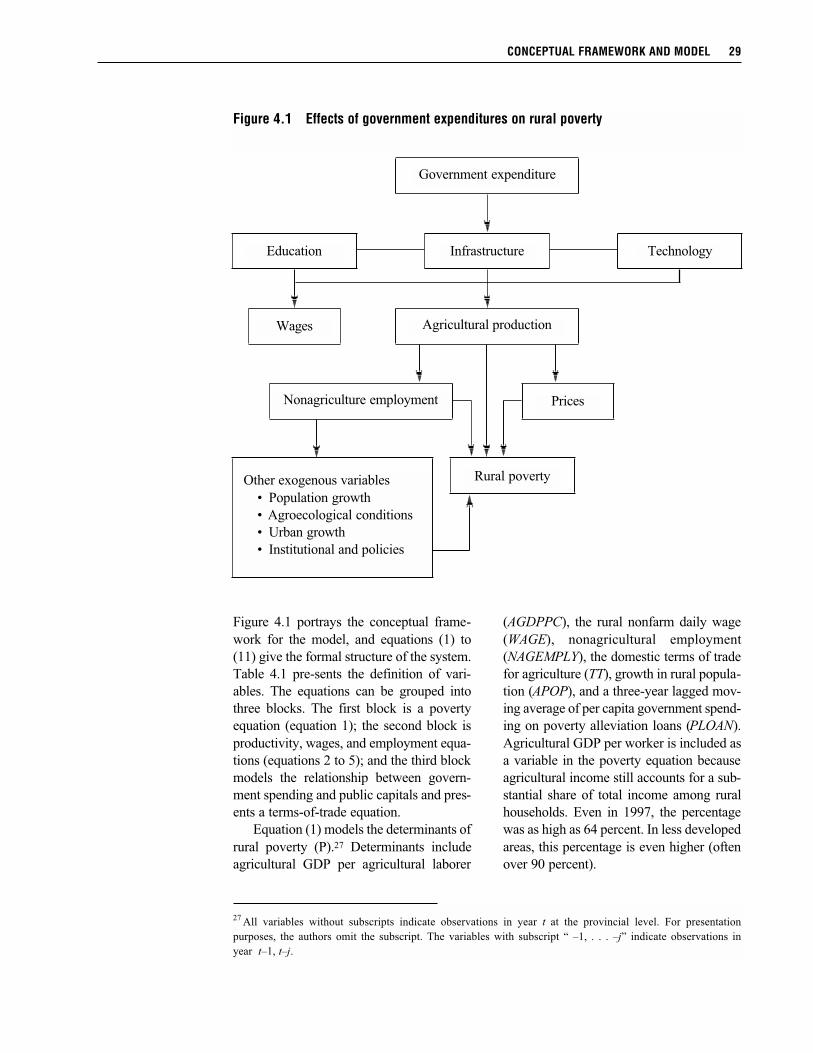
Figure 4.1 portrays the conceptual frame-
work for the model, and equations (1) to
(11) give the formal structure of the system.
Table 4.1 pre-sents the definition of vari-
ables. The equations can be grouped into
three blocks. The first block is a poverty
equation (equation 1); the second block is
productivity, wages, and employment equa-
tions (equations 2 to 5); and the third block
models the relationship between govern-
ment spending and public capitals and pres-
ents a terms-of-trade equation.
Equation (1) models the determinants of
rural poverty (P).27 Determinants include
agricultural GDP per agricultural laborer
(AGDPPC), the rural nonfarm daily wage
(WAGE), nonagricultural employment
(NAGEMPLY), the domestic terms of trade
for agriculture (TT), growth in rural popula-
tion (APOP), and a three-year lagged mov-
ing average of per capita government spend-
ing on poverty alleviation loans (PLOAN).
Agricultural GDP per worker is included as
a variable in the poverty equation because
agricultural income still accounts for a sub-
stantial share of total income among rural
households. Even in 1997, the percentage
was as high as 64 percent. In less developed
areas, this percentage is even higher (often
over 90 percent).
CONCEPTUAL FRAMEWORK AND MODEL 29
Figure 4.1 Effects of government expenditures on rural poverty
Government expenditure
InfrastructureEducation Technology
Wages Agricultural production
Nonagriculture employment Prices
Rural povertyOther exogenous variables
• Population growth
• Agroecological conditions
• Urban growth
• Institutional and policies
27 All variables without subscripts indicate observations in year t at the provincial level. For presentation
purposes, the authors omit the subscript. The variables with subscript “ –1, . . . –j” indicate observations in
year t–1, t–j.
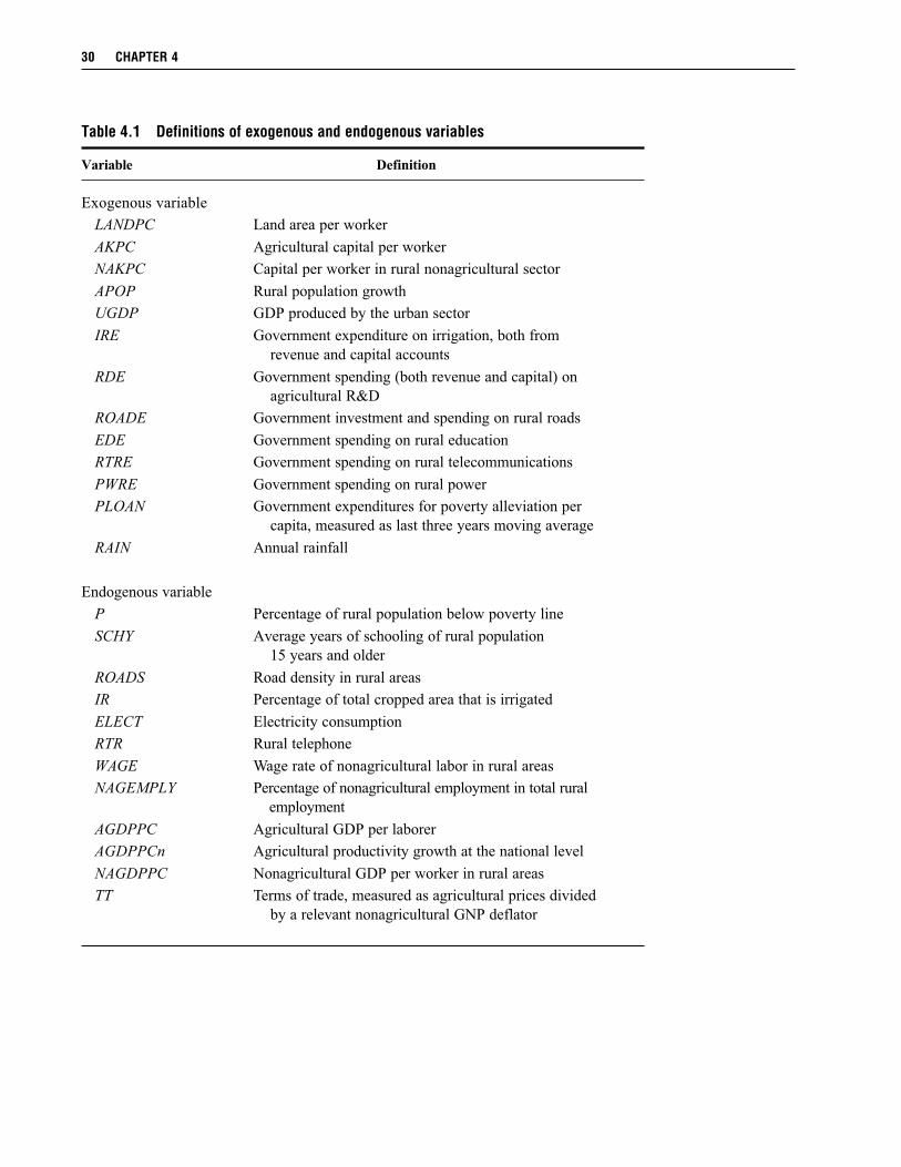
30 CHAPTER 4
Table 4.1 Definitions of exogenous and endogenous variables
Variable Definition
Exogenous variable
LANDPC Land area per worker
AKPC Agricultural capital per worker
NAKPC Capital per worker in rural nonagricultural sector
APOP Rural population growth
UGDP GDP produced by the urban sector
IRE Government expenditure on irrigation, both from
revenue and capital accounts
RDE Government spending (both revenue and capital) on
agricultural R&D
ROADE Government investment and spending on rural roads
EDE Government spending on rural education
RTRE Government spending on rural telecommunications
PWRE Government spending on rural power
PLOAN Government expenditures for poverty alleviation per
capita, measured as last three years moving average
RAIN Annual rainfall
Endogenous variable
P Percentage of rural population below poverty line
SCHY Average years of schooling of rural population
15 years and older
ROADS Road density in rural areas
IR Percentage of total cropped area that is irrigated
ELECT Electricity consumption
RTR Rural telephone
WAGE Wage rate of nonagricultural labor in rural areas
NAGEMPLY Percentage of nonagricultural employment in total rural
employment
AGDPPC Agricultural GDP per laborer
AGDPPCn Agricultural productivity growth at the national level
NAGDPPC Nonagricultural GDP per worker in rural areas
TT Terms of trade, measured as agricultural prices divided
by a relevant nonagricultural GNP deflator
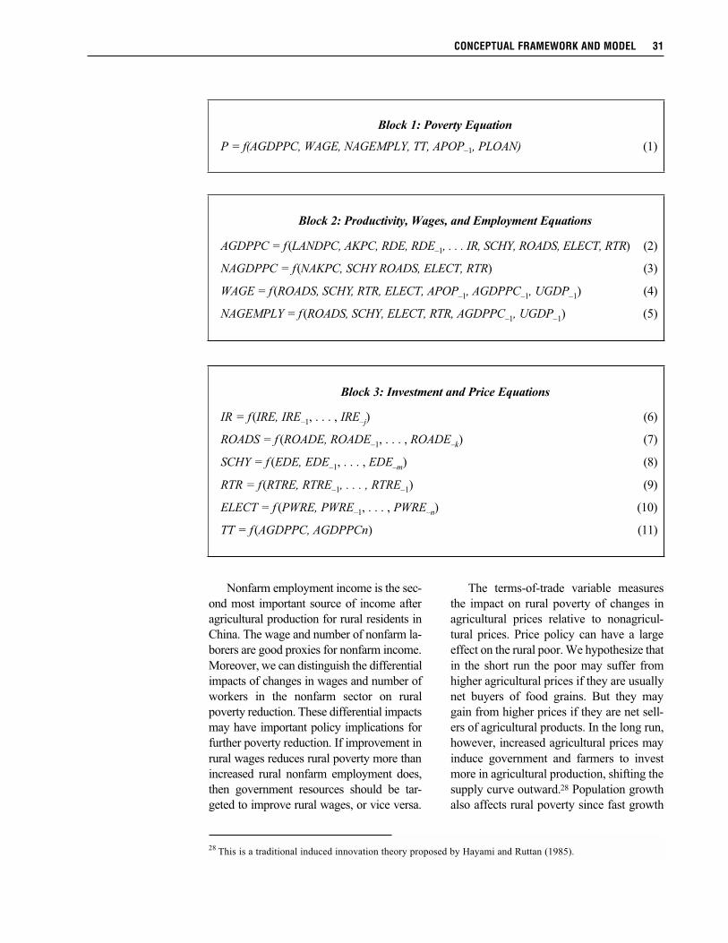
CONCEPTUAL FRAMEWORK AND MODEL 31
Nonfarm employment income is the sec-
ond most important source of income after
agricultural production for rural residents in
China. The wage and number of nonfarm la-
borers are good proxies for nonfarm income.
Moreover, we can distinguish the differential
impacts of changes in wages and number of
workers in the nonfarm sector on rural
poverty reduction. These differential impacts
may have important policy implications for
further poverty reduction. If improvement in
rural wages reduces rural poverty more than
increased rural nonfarm employment does,
then government resources should be tar-
geted to improve rural wages, or vice versa.
The terms-of-trade variable measures
the impact on rural poverty of changes in
agricultural prices relative to nonagricul-
tural prices. Price policy can have a large
effect on the rural poor. We hypothesize that
in the short run the poor may suffer from
higher agricultural prices if they are usually
net buyers of food grains. But they may
gain from higher prices if they are net sell-
ers of agricultural products. In the long run,
however, increased agricultural prices may
induce government and farmers to invest
more in agricultural production, shifting the
supply curve outward.28 Population growth
also affects rural poverty since fast growth
Block 1: Poverty Equation
P = f(AGDPPC, WAGE, NAGEMPLY, TT, APOP–1, PLOAN) (1)
Block 2: Productivity, Wages, and Employment Equations
AGDPPC = f (LANDPC, AKPC, RDE, RDE–1, . . . IR, SCHY, ROADS, ELECT, RTR) (2)
NAGDPPC = f(NAKPC, SCHY ROADS, ELECT, RTR) (3)
WAGE = f (ROADS, SCHY, RTR, ELECT, APOP–1, AGDPPC–1, UGDP–1) (4)
NAGEMPLY = f (ROADS, SCHY, ELECT, RTR, AGDPPC–1, UGDP–1) (5)
Block 3: Investment and Price Equations
IR = f (IRE, IRE–1, . . . , IRE–j) (6)
ROADS = f (ROADE, ROADE–1, . . . , ROADE–k) (7)
SCHY = f (EDE, EDE–1, . . . , EDE–m) (8)
RTR = f (RTRE, RTRE–1, . . . , RTRE–1) (9)
ELECT = f (PWRE, PWRE–1, . . . , PWRE–n) (10)
TT = f (AGDPPC, AGDPPCn) (11)
28 This is a traditional induced innovation theory proposed by Hayami and Ruttan (1985).
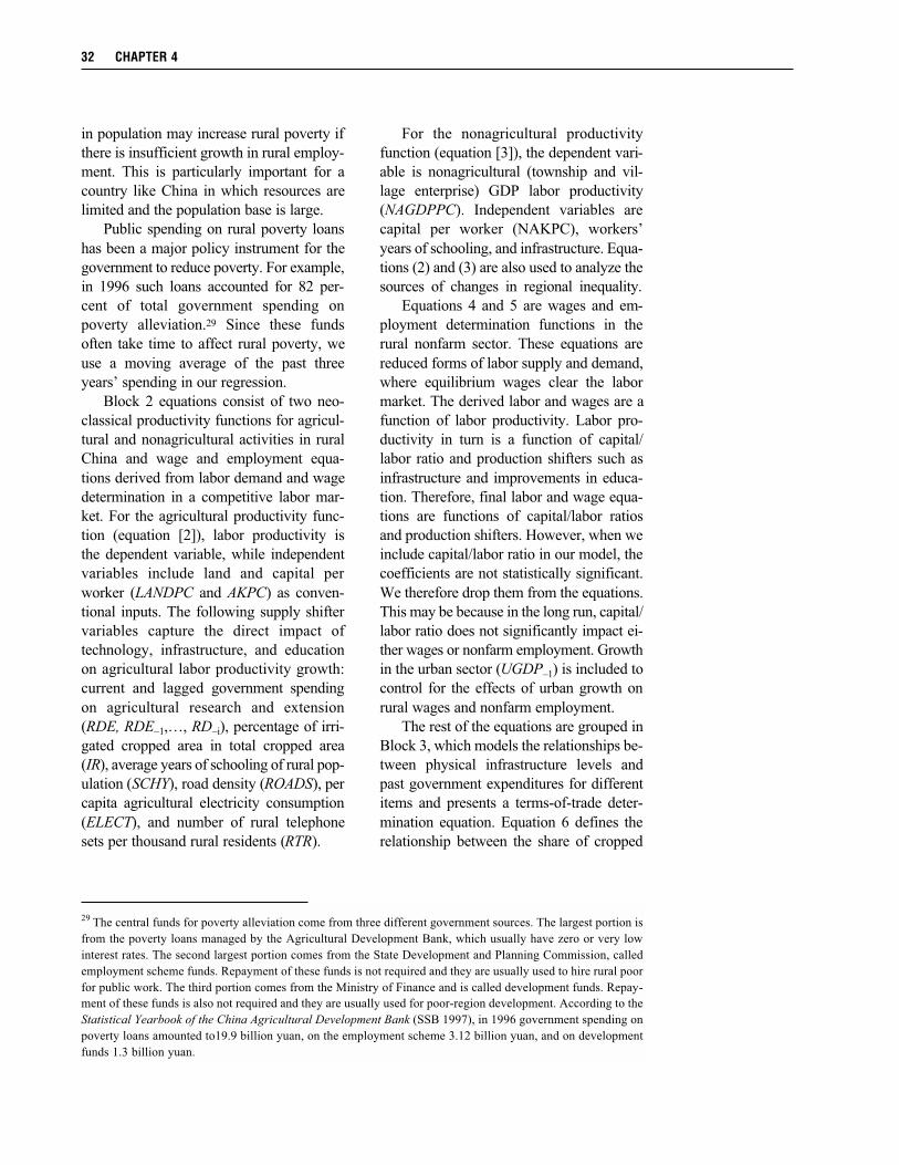
32 CHAPTER 4
in population may increase rural poverty if
there is insufficient growth in rural employ-
ment. This is particularly important for a
country like China in which resources are
limited and the population base is large.
Public spending on rural poverty loans
has been a major policy instrument for the
government to reduce poverty. For example,
in 1996 such loans accounted for 82 per-
cent of total government spending on
poverty alleviation.29 Since these funds
often take time to affect rural poverty, we
use a moving average of the past three
years’ spending in our regression.
Block 2 equations consist of two neo-
classical productivity functions for agricul-
tural and nonagricultural activities in rural
China and wage and employment equa-
tions derived from labor demand and wage
determination in a competitive labor mar-
ket. For the agricultural productivity func-
tion (equation [2]), labor productivity is
the dependent variable, while independent
variables include land and capital per
worker (LANDPC and AKPC) as conven-
tional inputs. The following supply shifter
variables capture the direct impact of
technology, infrastructure, and education
on agricultural labor productivity growth:
current and lagged government spending
on agricultural research and extension
(RDE, RDE–1,…, RD–i), percentage of irri-
gated cropped area in total cropped area
(IR), average years of schooling of rural pop-
ulation (SCHY), road density (ROADS), per
capita agricultural electricity consumption
(ELECT), and number of rural telephone
sets per thousand rural residents (RTR).
For the nonagricultural productivity
function (equation [3]), the dependent vari-
able is nonagricultural (township and vil-
lage enterprise) GDP labor productivity
(NAGDPPC). Independent variables are
capital per worker (NAKPC), workers’
years of schooling, and infrastructure. Equa-
tions (2) and (3) are also used to analyze the
sources of changes in regional inequality.
Equations 4 and 5 are wages and em-
ployment determination functions in the
rural nonfarm sector. These equations are
reduced forms of labor supply and demand,
where equilibrium wages clear the labor
market. The derived labor and wages are a
function of labor productivity. Labor pro-
ductivity in turn is a function of capital/
labor ratio and production shifters such as
infrastructure and improvements in educa-
tion. Therefore, final labor and wage equa-
tions are functions of capital/labor ratios
and production shifters. However, when we
include capital/labor ratio in our model, the
coefficients are not statistically significant.
We therefore drop them from the equations.
This may be because in the long run, capital/
labor ratio does not significantly impact ei-
ther wages or nonfarm employment. Growth
in the urban sector (UGDP–1) is included to
control for the effects of urban growth on
rural wages and nonfarm employment.
The rest of the equations are grouped in
Block 3, which models the relationships be-
tween physical infrastructure levels and
past government expenditures for different
items and presents a terms-of-trade deter-
mination equation. Equation 6 defines the
relationship between the share of cropped
29 The central funds for poverty alleviation come from three different government sources. The largest portion is
from the poverty loans managed by the Agricultural Development Bank, which usually have zero or very low
interest rates. The second largest portion comes from the State Development and Planning Commission, called
employment scheme funds. Repayment of these funds is not required and they are usually used to hire rural poor
for public work. The third portion comes from the Ministry of Finance and is called development funds. Repay-
ment of these funds is also not required and they are usually used for poor-region development. According to the
Statistical Yearbook of the China Agricultural Development Bank (SSB 1997), in 1996 government spending on
poverty loans amounted to19.9 billion yuan, on the employment scheme 3.12 billion yuan, and on development
funds 1.3 billion yuan.
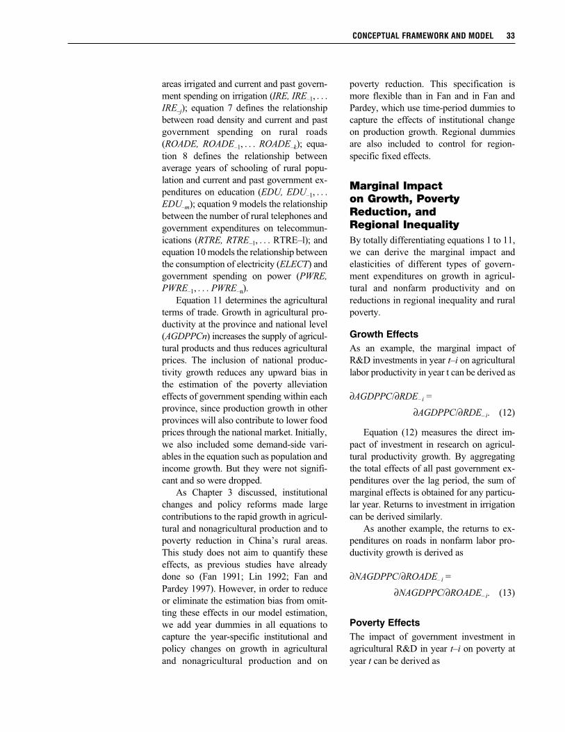
areas irrigated and current and past govern-
ment spending on irrigation (IRE, IRE–1, . . .
IRE–j); equation 7 defines the relationship
between road density and current and past
government spending on rural roads
(ROADE, ROADE–1, . . . ROADE–k); equa-
tion 8 defines the relationship between
average years of schooling of rural popu-
lation and current and past government ex-
penditures on education (EDU, EDU–1, . . .
EDU–m); equation 9 models the relationship
between the number of rural telephones and
government expenditures on telecommun-
ications (RTRE, RTRE–1, . . . RTRE–l); and
equation 10 models the relationship between
the consumption of electricity (ELECT) and
government spending on power (PWRE,
PWRE–1, . . . PWRE–n).
Equation 11 determines the agricultural
terms of trade. Growth in agricultural pro-
ductivity at the province and national level
(AGDPPCn) increases the supply of agricul-
tural products and thus reduces agricultural
prices. The inclusion of national produc-
tivity growth reduces any upward bias in
the estimation of the poverty alleviation
effects of government spending within each
province, since production growth in other
provinces will also contribute to lower food
prices through the national market. Initially,
we also included some demand-side vari-
ables in the equation such as population and
income growth. But they were not signifi-
cant and so were dropped.
As Chapter 3 discussed, institutional
changes and policy reforms made large
contributions to the rapid growth in agricul-
tural and nonagricultural production and to
poverty reduction in China’s rural areas.
This study does not aim to quantify these
effects, as previous studies have already
done so (Fan 1991; Lin 1992; Fan and
Pardey 1997). However, in order to reduce
or eliminate the estimation bias from omit-
ting these effects in our model estimation,
we add year dummies in all equations to
capture the year-specific institutional and
policy changes on growth in agricultural
and nonagricultural production and on
poverty reduction. This specification is
more flexible than in Fan and in Fan and
Pardey, which use time-period dummies to
capture the effects of institutional change
on production growth. Regional dummies
are also included to control for region-
specific fixed effects.
Marginal Impacton Growth, PovertyReduction, andRegional InequalityBy totally differentiating equations 1 to 11,
we can derive the marginal impact and
elasticities of different types of govern-
ment expenditures on growth in agricul-
tural and nonfarm productivity and on
reductions in regional inequality and rural
poverty.
Growth EffectsAs an example, the marginal impact of
R&D investments in year t–i on agricultural
labor productivity in year t can be derived as
∂AGDPPC/∂RDE– i =
∂AGDPPC/∂RDE– i. (12)
Equation (12) measures the direct im-
pact of investment in research on agricul-
tural productivity growth. By aggregating
the total effects of all past government ex-
penditures over the lag period, the sum of
marginal effects is obtained for any particu-
lar year. Returns to investment in irrigation
can be derived similarly.
As another example, the returns to ex-
penditures on roads in nonfarm labor pro-
ductivity growth is derived as
∂NAGDPPC/∂ROADE– i =
∂NAGDPPC/∂ROADE– i. (13)
Poverty EffectsThe impact of government investment in
agricultural R&D in year t–i on poverty at
year t can be derived as
CONCEPTUAL FRAMEWORK AND MODEL 33
34 CHAPTER 4
∂P/∂RDE– i = (∂P/∂AGDPPC) (∂AGDPPC/∂RDE– i)
+ (∂P/∂WAGE) (∂WAGE/∂AGDPPC) (∂AGDPPC/∂RDE– i)
+ (∂P/∂NAGEMPLY) (∂NAGEMPLY/∂AGDPPC) (∂AGDPPC/∂RDE–i)
+ (∂P/∂TT) (∂TT/∂AGDPPC) (∂AGDPPC/∂RDE– i). (14)
The first term on the right-hand side of equation 14 captures the impact on poverty of
government investments in R&D through yield-enhancing technologies such as improved
varieties, and therefore agricultural labor productivity. Increased agricultural labor productiv-
ity also affects poverty through changes in rural nonfarm wages and employment and relative
prices, which are captured in the remaining terms on the right of the equation.
As with government investments in agricultural R&D, the impact of government invest-
ments in irrigation is captured through improved productivity, rural wages and nonfarm
employment, and relative prices.
The impact of government investments in rural roads in year t–k on poverty in year t is
derived as
∂P/∂ROADE–k = (∂P/∂AGDPPC)(∂AGGDPC/∂ROADS)(∂ROADS/∂ROADE– k)
+ (∂P/∂WAGE) (∂WAGE/∂AGDPPC)(∂AGDPPC/∂ROADS)
(∂ROADS/∂ROADE– k)
+ (∂P/∂NAGEMPLY) (∂NAGEMPLY/∂AGDPPC)(∂AGDPPC/∂ROADS)
(∂ROADS/∂ROADE– k)
+ (∂P/∂TT) (∂TT/∂AGDPPC)(∂AGDPPC/∂ROADE– i)
+ (∂P/∂WAGE) (∂WAGE/∂ROADS) (∂ROADS/∂ROADE–k)
+ (∂P/∂NAGEMPLY)(∂NAGEMPLY/∂ROADS) (∂ROADS/∂ROADE– k). (15)
The first term on the right side of equa-
tion 15 measures the direct effects on pov-
erty of improved productivity attributable
to greater road density. Terms 2, 3, and 4
are the indirect effects of improved produc-
tivity through changes in rural nonfarm
wages, employment, and prices. Terms 5
and 6 capture the direct effects on poverty
of higher nonfarm wages and greater non-
agricultural employment opportunities aris-
ing from government investment in roads.
We can similarly derive the impact on rural
poverty of increased investment in telecom-
munications, electricity, and education.
Impact on Regional InequalityTo decompose the sources of changes in
regional inequality of labor productivity,
we consider equations (2) and (3) in the
following double-log form:
(16)
where all the variables are in logarithms, y
is the dependent variable and xi represents a
set of independent variables. An error term
ε is added to represent stochastic shocks to
output and is assumed to be unrelated to
y = a +∑ βi xi + ε ,i
CONCEPTUAL FRAMEWORK AND MODEL 35
where σ2 (y) is the variance of y and cov(y,• )
represents the covariance of y with other
variables. Since none of the variables on
the right side of equation 16 is correlated
with the error term, the covariance of y and
ε is equal to the variance of ε. Considering
that y is already in logarithmic form, is a
standard inequality measure known as the
logarithmic variance (Cowell 1995), hav-
ing the property of invariance to scale.
According to Shorrocks, the covariance
terms on the right side of 17 can be re-
garded as the contributions of the factor
components to total inequality.
Using estimates from equations 2 and 3
and applying the above decomposition
method, we can quantify the contributions
of various public investments on regional
inequality in both agricultural and nonagri-
cultural labor productivities. Moreover, we
can calculate the impact of public invest-
ments on regional inequality in total labor
productivity. For this purpose, we further
write total rural labor productivity as
Y = a1Y1 + a2Y2, (18)
where Y, Y1, and Y2 are total, agricultural,
and nonagricultural productivities, respec-
tively; a1 and a2 are, respectively, the shares
of agricultural and nonagricultural laborers
in total labor. Under six axioms proposed
by Shorrocks, a broad class of inequality
measures such as Gini coefficient, the
Atkinson index, and the logarithmic vari-
ance index can be written as
If we still use the logarithmic variance as an
inequality measure, then we can substitute
the estimated variance for Y1 and Y2 from
17 into 19 to obtain the contributions of
public inputs to total inequality.
(17)
the other variables. Following Shorrocks
(1982), the variance of y in equation 16 can
be decomposed as
(19)
where
∑cov (y, βi xi) + cov(y,ε)i
∑k
σ 2 (y) =
=
=
βi cov (y, xi) + cov(y,ε )
∑k
βi cov (y, xi) + σ 2 (ε),
I(Y) = s1I(a1Y1) + s2I(a2Y2),
s1=
cov(Y,a1Y1)
σ 2 (Y) σ 2 (Y)
cov(Y,a2Y2)s
2=, .
C H A P T E R 5
Data, Estimation, and Results
T his chapter describes the data and discusses the estimation technique and estimation re-
sults. It further details the calculation and analysis of the marginal returns derived from
additional units of expenditure on various types of public capitals and in different regions.
Data
Poverty
There are several estimates of rural poverty in China. Official statistics indicate that the num-
ber of poor declined to about 50 million by 1997 (MOA, China Agricultural Development
Report 1998). World Bank estimates (Piazza and Liang 1998) are similar to Chinese official
statistics. A third set of estimates, based on a much higher poverty line (Ravallion and Chen
1997), shows a far greater proportion of the total population subject to poverty, with a poverty
incidence of 60 percent in 1978 and 22 percent in 1995. However, the declining trend of rural
poverty in this last set of estimates is steeper than that in the official Chinese statistics. Khan,
using samples of the household survey, obtained 35.1 percent for 1988 and 28.6 percent for
1995.30 Although these poverty rates are higher than the official rates, the change over time
differs little from the official statistics.
The present study uses provincial-level poverty data from official sources. Few scholars
have reported their estimates by province. Khan estimated provincial poverty indicators (both
head count ratio and poverty gap index) for 1988 and 1995 using the household survey data.
To test the sensitivity of our estimated results, we first used both official statistics and Khan’s
estimates, obtaining similar results, largely because the two sets of poverty figures share
similar trends. Our final results are based on the official data simply because poverty data are
available by province for more years.
Agricultural and Nonagricultural GDPBoth nominal gross domestic product (GDP) and real GDP growth indices for various sectors
are available from the The Gross Domestic Product of China (SSB 1997a). Data sources and
construction of national GDP estimates were also published by the State Statistical Bureau
(SSB) in Calculation Methods of China’s Annual GDP (SSB 1997b). According to this
publication, the SSB used the U.N. standard SNA (system of national accounts) definitions to
estimate GDP for 29 provinces by three economic sectors (primary, secondary, and tertiary) in
30 The dataset included 10,258 rural households in 1998 and 7,998 in 1995.
36
mainland China for the period 1952–95.
Since 1995, the China Statistical Yearbook
has published GDP data every year for each
province by the same three sectors. Both
nominal and real growth rates are available
from SSB publications.
The agricultural sector is equivalent to
the primary sector used by the SSB. We use
the following procedures to construct GDP
for the nonagricultural sector in rural areas:
Until 1996, China published the value of
annual gross production for rural industry
and services. In 1996, it began to publish
value-added figures. The definition of value
added is equivalent to the GDP data. The
Ministry of Agriculture published data on
both gross production value and value
added for rural industry (including con-
struction) and services in the China Agri-
cultural Yearbook 1996. The data on nomi-
nal value added for rural industry and serv-
ices prior to 1995 were estimated using
the growth rate of gross production value
and 1995 value-added figures, assuming
no change in the ratio of value added to
gross production value.
GDP for rural industry was subtracted
from GDP for industry as a whole (or the
secondary sector as classified by the SSB)
to obtain GDP for urban industry. Similarly,
GDP for rural services was subtracted from
the aggregate service sector GDP (or the
tertiary sector as classified by the SSB) to
obtain GDP for the urban service sector.
GDP for rural enterprise is the sum of GDP
for rural industry and rural services.
The implicit GDP deflators by province
for the three sectors are estimated by divid-
ing nominal GDP by real GDP. These de-
flators are then used to deflate nominal
GDP for rural industry and services to ob-
tain their GDP in real terms.
LaborAgricultural labor is measured in stock
terms as the number of persons engaged in
agricultural production at the end of each
year. The data prior to 1978 were avail-
able in the SSB’s Historical Statistical
Materials for Provinces, Autonomous Re-
gions and Municipalities (1949–1990).
The data after 1977 were taken from vari-
ous issues of the China Agricultural Year-
book (MOA), the China Statistical Year-
book (SSB), and the China Rural Statisti-
cal Yearbook (SSB).
The labor input for the nonfarm sector is
calculated simply by subtracting agricul-
tural labor from total rural labor.
Capital StockCapital stocks for the agricultural and non-
agricultural sectors in rural areas are calcu-
lated from data on gross capital formation
and annual fixed asset investment. For the
three sectors classified, the SSB (1997)
published data on gross capital formation
by province after 1978. Gross capital for-
mation is defined as the value of fixed as-
sets and inventory acquired minus the value
of fixed assets and inventory disposed. To
construct a capital stock series from data on
capital formation, we use the following pro-
cedure: define the capital stock in time t as
the stock in time t–1 plus investment minus
depreciation,
Kt = It + (1–δ) Kt–1, (20)
where Kt is the capital stock in year t, It is
gross capital formation in year t, and δ is the
depreciation rate. China Statistical Year-
book (SSB 1995) reports the depreciation
rate of fixed assets of state-owned enter-
prises for industry, railways, communica-
tions, commerce, and grain for the period
1952–92. We use the rates for grain and
commerce for agriculture and services,
respectively. After 1992, the SSB ceased
to report official depreciation rates. For
the years after 1992 we used the 1992
depreciation rates.
To obtain initial values for the capital
stock, we used a procedure similar to Kohli
(1982). That is, we assume that prior to
1978 real investment grew at a steady rate
(r), which is assumed to be the same as the
rate of growth of real GDP from 1952 to
1977. Thus,
DATA, ESTIMATION, AND RESULTS 37
This approach ensures that the 1978
value of the capital stock is independent of
the 1978–95 data used in our analysis.
Moreover, given the relatively small capital
stock in 1978 and the high levels of invest-
ment, the estimates for later years are not
sensitive to the 1978 benchmark value of
the capital stock.
Estimates of capital stocks for rural in-
dustry and services are constructed using
the annual fixed asset investment by prov-
ince from 1978 to 1995. These are from the
China Statistical Yearbook (SSB, various
years) and the China Fixed Asset Invest-
ment Statistical Materials, 1950–95 (SSB,
1996). Initial values are calculated using
equation 21, but the growth rate of real
investment prior to 1978 is assumed to be
4 percent. Again, the initial capital stock is
low so the estimated series is not sensitive
to the benchmark starting value.
Capital stock for rural industry is sub-
tracted from that of total industry (or sec-
ondary industry as classified by the SSB) to
obtain capital stock for the urban industrial
sector. Similarly, capital stock for rural
services is subtracted from the aggregate
service sector (or tertiary sector as classi-
fied by the SSB) to obtain the capital stock
for the urban service sector. Finally, capital
stock for rural enterprise is the sum of cap-
ital stocks for rural industry and services.
Prior to constructing capital stocks for
each sector, annual data on capital forma-
tion and fixed asset investment was deflated
by a capital investment deflator. The SSB
began to publish provincial price indices for
fixed asset investment in 1987. Prior to
1987, we use the national price index of
construction materials to proxy the capital
investment deflator.
Research and Development(R&D) ExpendituresPublic investment in agricultural R&D is
accounted for in the total national science
and technology budget. The sources of agri-
cultural R&D investment are different gov-
ernment agencies. Science and technology
commissions at different levels of govern-
ment allocate funds to national, provincial,
and prefectural institutes, primarily as core
support. These funds are mainly used by in-
stitutes to cover researchers’ salaries, bene-
fits, and administrative expenses. Project
funds come primarily from other sources, in-
cluding departments of agriculture, research
foundations, and international donors. Re-
cently, revenues generated from commercial
activities (development income) became an
important source of revenue for the research
institutes. The research expenditures re-
ported in this study include only those ex-
penses used to directly support agricultural
research. The data reported here are from
Fan and Pardey (1992) and various publica-
tions from the Government Science and
Technology Commission and the State
Statistical Bureau. Research expenditures
and personnel numbers include those from
research institutions at national, provincial,
and prefectural levels, as well as agricultural
universities (only the research part).
When calculating returns to R&D in-
vestment, expenditures on agricultural re-
search as well as extension at the national
and sub-national levels are used as total
R&D spending. This implicitly assumes
that research conducted at the national level
affects each province’s production in pro-
portion to the province’s research expendi-
tures, and the impact of extension con-
ducted in each province is proportional to
research impact.
Irrigation ExpendituresProvincial irrigation expenditures refer to
total government fiscal expenditures in con-
struction of reservoirs, irrigation and
drainage systems, and flood and lodging
prevention, as well as maintenance of these
systems. However, government reports of
such data are available only after 1980 in
the China Water Conservancy Yearbook
(various years). Prior to 1979, the Ministry
38 CHAPTER 5
(21)K1978 =(ä + r)
.I1978
of Water Conservancy reported total expen-
diture (not by item) on reservoirs, irrigation
and drainage systems, flood and lodging
prevention, water supply, and hydropower
(Ministry of Water Conservancy 1980). This
spending item is much broader than irriga-
tion, as it also includes urban water supply,
flood control, and hydropower generation.
To calculate the cost solely of irrigation
prior to 1979, we use the percentage of irri-
gation spending in total expenditures on
water conservancy in 1980.
Education ExpendituresProvincial expenditures for primary- and
middle-school education in rural areas after
1990 are reported in the China Education
Yearbook (Ministry of Education, various
years) and the China Education Expendi-
ture Yearbook (SSB). Expenditures prior to
1990 are extrapolated using the percentage
of rural students in total students. Since edu-
cation expenditure per student in urban areas
is higher than that in rural areas, we use the
cost difference in 1990 to adjust down the
total education expenditures in rural areas.
Road ExpendituresRoad expenditures are reported in China
Fixed Asset Investment Statistical Materi-
als, 1950–95 (SSB 1996) and the China
Transportation Yearbook (Ministry of Trans-
portation, various years). However, there is
no breakdown between rural and urban road
expenditures. We use the percentage of the
length of rural roads in total length of roads
to extrapolate the cost of rural roads by
assuming the unit cost of rural road con-
struction is one third that of urban roads
(Ministry of Transportation 1995).
Power ExpendituresProvincial power expenditures are available
in China Fixed Asset Investment Statistical
Materials, 1950–95 (SSB 1996) and the
China Power Yearbook (Ministry of Elec-
tric Power, various years). We use the unit
cost of electricity per kilowatt to calculate
power expenditures for rural areas.
Telecommunications ExpendituresTelecommunications expenditures by prov-
ince are available in China Fixed Asset
Investment Statistical Materials, 1950–95
(SSB 1996) and of the China Transporta-
tion Yearbook (Ministry of Transportation,
various years). However, similar to expen-
ditures on roads and power, there is no
breakdown between rural and urban expen-
ditures. We use the number of telephones in
rural and urban areas to extrapolate the cost
of rural telecommunications.
Rural EducationWe use the percentage of population with
different education levels to calculate the
average years of schooling as our education
variable, assuming 0 years for a person who
is illiterate or semi-illiterate, 5 years for pri-
mary-school education, 8 years for a junior
high-school education, 12 years for a high-
school education, 13 years for a professional-
school education, and 16 years for college
and above education. The population census
and the Ministry of Education report educa-
tion levels for population above age 7.
RoadsThe road variable is measured as road den-
sity, road length in kilometers per thousand
square kilometers of geographic area. The
length of total roads by province is reported
in the China Statistical Yearbook (SSB, var-
ious years) and the China Transportation
Yearbook (Ministry of Transportation),
while the length of rural roads in the 1980s
is reported in of the China Rural Statistical
Yearbook (SSB, various years). In more re-
cent years, the China Rural Statistical Year-
book stopped reporting rural roads. We
therefore use the trend of total length of
roads (except highways) to extrapolate the
length of rural roads for the years in which
data are not available.
ElectricityTotal rural electricity consumption for both
production and residential uses by province
are available in of the China Rural Statisti-
DATA, ESTIMATION, AND RESULTS 39
40 CHAPTER 5
cal Yearbook and the China Agricultural
Yearbook (MOA). In more recent years,
the China Rural Energy Yearbook (SSB,
various years) (MOA 1995–2000) began
publishing the use of electricity separately
for residential and production purposes
by province. We use this newly available
information to backcast the different use
by province for earlier years.
Rural TelephonyNumber of rural telephones is used as a
proxy for the development of rural tele-
communications. The number of rural tele-
phones by province is published in of the
China Rural Statistical Yearbook (SSB,
various years), the China Statistical Year-
book (SSB, various years), and the China
Transportation Yearbook (Ministry of Trans-
portation, various years).
Model Estimation
Functional Form and EstimationProcedure
We use double-log functional forms for all
equations in the system. More flexible func-
tional forms such as translog or quadratic
impose fewer restrictions on estimated pa-
rameters, but many coefficients are not sta-
tistically significant due to multicollinearity
problems among various interaction vari-
ables. For the system equations, we use the
full information maximum-likelihood esti-
mation technique.
Since our provincial poverty data are
available only for seven years (1985–89,
1991, and 1996) a two-step procedure is
used in estimating the full equations
system. The first step involves estimating
all the equations except for the poverty
equation using the provincial-level data
from 1970 to 1997. Then the values of
AGDPPC, WAGE, and NAGEMPLY and
TT at the pro-vincial level are predicted
using the estimated parameters. The sec-
ond step estimates the poverty equation
using the predicted values of the independ-
ent variables at the provincial level based
on the available poverty data for 1985–89,
1991, and 1996. The advantage of this pro-
cedure is to fully use the information avail-
able for all non-poverty equations, thereby
increasing the reliability of estimates and
avoiding the endogeneity problem of the
poverty equation.
Lags and Distribution ofPublic InvestmentsGovernment investments in R&D, roads,
education, power, telecommunications, and
irrigation can have long lead times in
affecting agricultural production, and their
effects can be long term once they kick in.
Thus, one of the thornier problems to resolve
when including government investment
variables in a production or productivity
function concerns the choice of appropriate
lag structure. Most past studies use stock
variables, which are usually weighted aver-
ages of current and past government expen-
ditures on certain investments such as R&D.
But what weights and how many years’ lag
should be used in the aggregation are under
debate.31 Since the shape and length of
these investments are largely unknown, we
use a free-form lag structure in our analysis;
that is, we include current and past govern-
ment expenditures on certain investment
items such as R&D, irrigation, roads, power,
and education in the respective productiv-
ity, technology, infrastructure, and educa-
tion equations. Then we use statistical tools
to test and determine the appropriate length
of lag for each investment expenditure.
31 Alston, Craig, and Pardey (1998) argue that the research lag may be much longer than previously thought or
even infinite. But in many developing countries the national agricultural research systems are much younger than
those in developed countries (often 30 to 50 years old) and their research is of more the applied type. Therefore,
it is certain that research lags in developing countries are much shorter than those in developed countries.

DATA, ESTIMATION, AND RESULTS 41
Various procedures have been sug-
gested for determining the appropriate lag
length. The adjusted R2 and Akaike’s Infor-
mation Criteria (AIC) are often used by
economists (Greene 1993). This report sim-
ply uses the adjusted R2. Since R2 estimated
from the simultaneous system does not pro-
vide the correct information on the fitness
of the estimation, we use the adjusted R2
stimated from the single equation. The opti-
mal length is determined when adjusted R2
reaches a maximum. The AIC is similar in
spirit to the adjusted R2 in that it rewards
good fit but penalizes the loss of degrees
of freedom. The lags determined by the
adjusted R2 approach are 17, 14, 16, 12, and
17 years for R&D, irrigation, education,
power, and roads. These are generally very
short in comparison to those in the United
States (Alston, Craig, and Pardey 1998).
Another problem related to the estima-
tion of lag distribution is that independent
variables (for example, RDE, RDE–1,
RDE–2, . . . and RDE– i in the productivity
function) are often highly correlated, mak-
ing the estimated coefficients statistically
insignificant. A number of ways to tackle
this problem have been proposed. The most
popular is to use what are called polynomial
distributed lags, or PDLs. In a polynomial
distributed lag, the coefficients are all
required to lie on a polynomial of some
degree d. This analysis uses PDLs with de-
gree 2. In this case, we only need to esti-
mate three instead of i +1 parameters for the
lag distribution. For more detailed informa-
tion on this subject, refer to Davidson and
MacKinnon (1993). Once the lengths of
lags are determined, we estimate the simul-
taneous equation system with the PDLs and
appropriate lag length for each investment.
Estimation ResultsTable 5.1 presents the results of the systems
equation estimation. Most of the coeffi-
cients in the estimated system are statisti-
cally significant at the 10 percent confi-
dence level (one-tail test). Since we use the
double-log functional form, the estimated
coefficients are elasticities in their respec-
tive equations.
The estimated poverty equation (equa-
tion 1) supports the findings of many pre-
vious studies. Improvements in agricultural
productivity, higher agricultural wages, and
increased nonagricultural employment op-
portunities have all contributed signifi-
cantly to reducing poverty. The coefficient
of the terms-of-trade variable is negative
and statistically significant, meaning that
higher agricultural prices are good for the
poor. This is explained by the fact that most
poor farmers in China are net sellers of agri-
cultural products. When agricultural prices
rise, their incomes rise. This is in sharp con-
trast to India where the poor generally suf-
fer from higher agricultural prices because
they tend to be landless laborers and net
buyers of food grains (Fan, Hazell, and
Thorat 1999). In China, equal distribution
of land-use rights among households guar-
antees equal access to land, the result being
virtually no landless laborers in rural areas.
Although the population growth vari-
able is positively related to poverty, the
coefficient is not statistically significant.
Government spending on poverty allevia-
tion loans helps to reduce rural poverty, but
the coefficient of the variable is not statisti-
cally significant.32
The estimated agricultural labor pro-
ductivity function (equation 2) shows that
agricultural research and extension, roads,
32The authors also tried other specifications of the poverty equation. For example, instead of rural nonfarm
wages and employment, they included labor productivity of the nonfarm sector. The results were similar, how-
ever. They prefer the current specification because it permits modeling the separate effects of wages and
employment on rural poverty reduction.
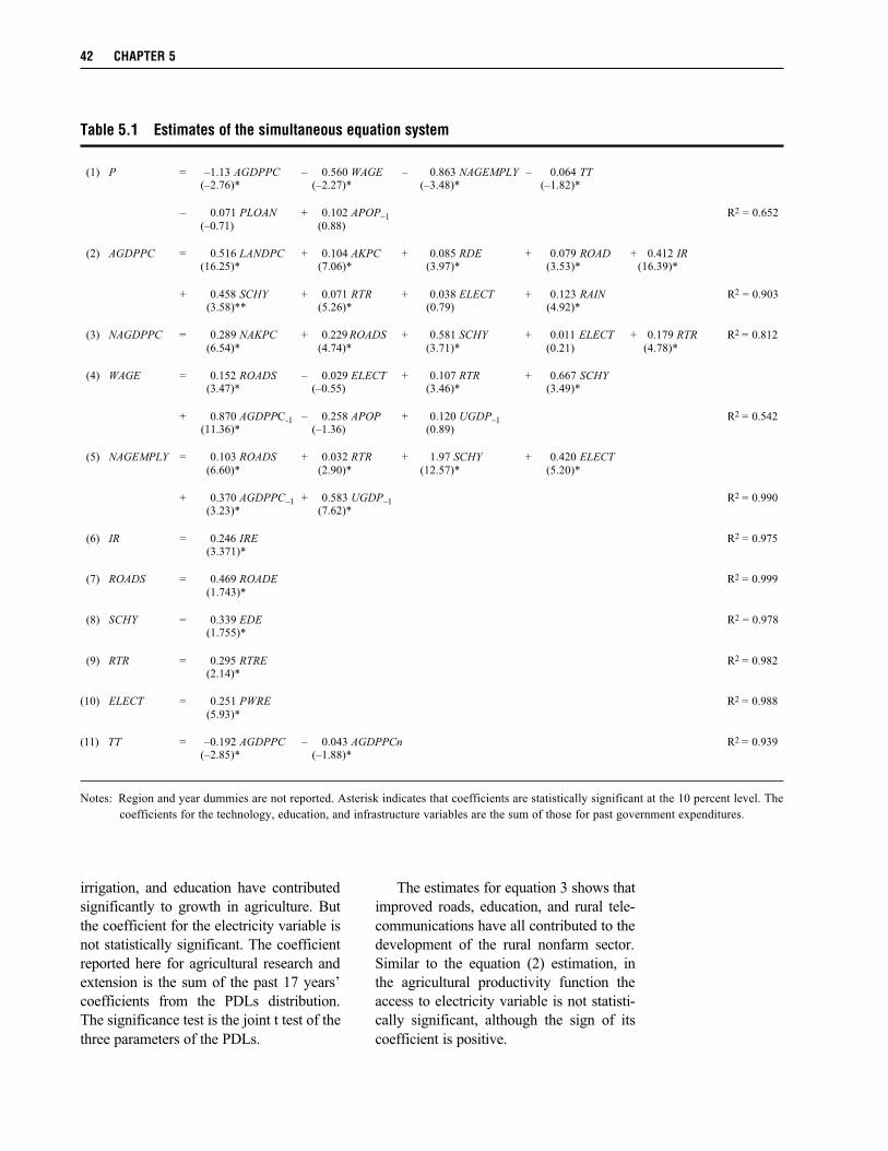
42 CHAPTER 5
irrigation, and education have contributed
significantly to growth in agriculture. But
the coefficient for the electricity variable is
not statistically significant. The coefficient
reported here for agricultural research and
extension is the sum of the past 17 years’
coefficients from the PDLs distribution.
The significance test is the joint t test of the
three parameters of the PDLs.
The estimates for equation 3 shows that
improved roads, education, and rural tele-
communications have all contributed to the
development of the rural nonfarm sector.
Similar to the equation (2) estimation, in
the agricultural productivity function the
access to electricity variable is not statisti-
cally significant, although the sign of its
coefficient is positive.
Table 5.1 Estimates of the simultaneous equation system
(1) P = –1.13 AGDPPC – 0.560 WAGE – 0.863 NAGEMPLY – 0.064 TT(–2.76)* (–2.27)* (–3.48)* (–1.82)*
– 0.071 PLOAN + 0.102 APOP–1 R2 = 0.652(–0.71) (0.88)
(2) AGDPPC = 0.516 LANDPC + 0.104 AKPC + 0.085 RDE + 0.079 ROAD + 0.412 IR(16.25)* (7.06)* (3.97)* (3.53)* (16.39)*
+ 0.458 SCHY + 0.071 RTR + 0.038 ELECT + 0.123 RAIN R2 = 0.903(3.58)** (5.26)* (0.79) (4.92)*
(3) NAGDPPC = 0.289 NAKPC + 0.229 ROADS + 0.581 SCHY + 0.011 ELECT + 0.179 RTR R2 = 0.812(6.54)* (4.74)* (3.71)* (0.21) (4.78)*
(4) WAGE = 0.152 ROADS – 0.029 ELECT + 0.107 RTR + 0.667 SCHY(3.47)* (–0.55) (3.46)* (3.49)*
+ 0.870 AGDPPC-1 – 0.258 APOP + 0.120 UGDP–1 R2 = 0.542(11.36)* (–1.36) (0.89)
(5) NAGEMPLY = 0.103 ROADS + 0.032 RTR + 1.97 SCHY + 0.420 ELECT
(6.60)* (2.90)* (12.57)* (5.20)*
+ 0.370 AGDPPC–1 + 0.583 UGDP–1 R2 = 0.990(3.23)* (7.62)*
(6) IR = 0.246 IRE R2 = 0.975(3.371)*
(7) ROADS = 0.469 ROADE R2 = 0.999(1.743)*
(8) SCHY = 0.339 EDE R2 = 0.978(1.755)*
(9) RTR = 0.295 RTRE R2 = 0.982(2.14)*
(10) ELECT = 0.251 PWRE R2 = 0.988(5.93)*
(11) TT = –0.192 AGDPPC – 0.043 AGDPPCn R2 = 0.939(–2.85)* (–1.88)*
Notes: Region and year dummies are not reported. Asterisk indicates that coefficients are statistically significant at the 10 percent level. The
coefficients for the technology, education, and infrastructure variables are the sum of those for past government expenditures.
DATA, ESTIMATION, AND RESULTS 43
The estimates for equation 4 show that
rural nonfarm wages are determined mainly
by government investments in roads, edu-
cation, and telecommunications. An impor-
tant finding in this equation is that agricul-
tural labor productivity affects rural non-
farm wages significantly. But urban growth
has no statistically significant impact on
rural wages.
The estimates for equation 5 show that
improved rural roads, telecommunications,
electrification, and education have con-
tributed to growth in nonfarm employment.
Growth in agricultural productivity has
contributed significantly to the develop-
ment of rural nonfarm employment. In con-
trast to the wage equation, development in
the urban sector had significant impact on
rural nonfarm employment.
The estimated results for equations 6 to
10 show that government investments in
irrigation, roads, education, rural telecom-
munications, and power have contributed to
the improvement of irrigation, to the devel-
opment of roads, to rural education, to rural
communication, and to the increased use of
electricity. All the coefficients are statisti-
cally significant.
Finally, the estimated terms-of-trade
equation equation 11 confirms that in-
creases in agricultural productivity at the
local and national levels exerted a down-
ward pressure on agricultural prices, wors-
ening the terms of trade for agriculture.
The Effects of PublicInvestment
Marginal Effects on Growthand Poverty Reduction
Using equations 1 to 11 and the estimates in
Table 5.1, we can derive the marginal re-
turns to different types of government ex-
penditures in growth and reduction of rural
poverty as shown in equations 12 to 15. We
calculate marginal returns by different types
of investments in three regions.
Table 5.2 presents major development
indicators of these three regions. The
coastal region is the most developed with
the best infrastructure and human capital as
well as superior agroclimatic conditions.33
The western region is the least developed
and has poor natural resources and social
infrastructure. The central region falls in
between the other two.
Table 5.3 shows the marginal effects of
government spending on agricultural and
nonagricultural production and rural poverty
for the three regions and for China as a
whole. Effects are measured as the returns
in yuan or the number of poor brought out
of poverty per unit of spending in 1997. For
example, the returns to investments in irri-
gation are measured as yuan of additional
production or number of persons brought
out of poverty per one additional unit spent
on irrigation. These measures provide use-
ful information for comparing the relative
benefits of additional units of expenditure
on different items in different regions, par-
ticularly for setting future priorities for gov-
ernment expenditure to further increase
production and reduce rural poverty.
An important feature of the results in
Table 5.3 is that all production-enhancing
investments reduce poverty while at the
same time increasing agricultural and non-
agricultural GDP. However, there are siz-
able differences in production gains and
poverty reductions among the various ex-
penditure items and across regions.
For the country as a whole, government
expenditure on education had by far the
33The coastal region includes the following provinces: Hebei, Liaoning, Shandong, Jiangsu, Zhejiang, Fujian,
Guangdong, and Guangxi. The central region contains Shanxi, Inner Mongolia, Anhui, Jiangxi, Henan, Hubei,
and Hunan. The remaining provinces are classified as the western region. Tibet is excluded due to the lack of
data. Hainan is included in Guangdong Province. Beijing, Shanghai, and Tianjin are excluded because of their
small share of rural areas and population.
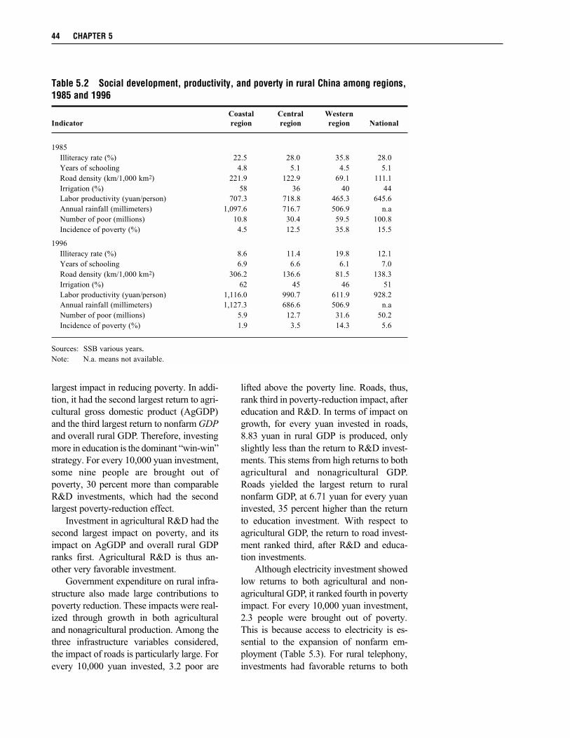
44 CHAPTER 5
largest impact in reducing poverty. In addi-
tion, it had the second largest return to agri-
cultural gross domestic product (AgGDP)
and the third largest return to nonfarm GDP
and overall rural GDP. Therefore, investing
more in education is the dominant “win-win”
strategy. For every 10,000 yuan investment,
some nine people are brought out of
poverty, 30 percent more than comparable
R&D investments, which had the second
largest poverty-reduction effect.
Investment in agricultural R&D had the
second largest impact on poverty, and its
impact on AgGDP and overall rural GDP
ranks first. Agricultural R&D is thus an-
other very favorable investment.
Government expenditure on rural infra-
structure also made large contributions to
poverty reduction. These impacts were real-
ized through growth in both agricultural
and nonagricultural production. Among the
three infrastructure variables considered,
the impact of roads is particularly large. For
every 10,000 yuan invested, 3.2 poor are
lifted above the poverty line. Roads, thus,
rank third in poverty-reduction impact, after
education and R&D. In terms of impact on
growth, for every yuan invested in roads,
8.83 yuan in rural GDP is produced, only
slightly less than the return to R&D invest-
ments. This stems from high returns to both
agricultural and nonagricultural GDP.
Roads yielded the largest return to rural
nonfarm GDP, at 6.71 yuan for every yuan
invested, 35 percent higher than the return
to education investment. With respect to
agricultural GDP, the return to road invest-
ment ranked third, after R&D and educa-
tion investments.
Although electricity investment showed
low returns to both agricultural and non-
agricultural GDP, it ranked fourth in poverty
impact. For every 10,000 yuan investment,
2.3 people were brought out of poverty.
This is because access to electricity is es-
sential to the expansion of nonfarm em-
ployment (Table 5.3). For rural telephony,
investments had favorable returns to both
Table 5.2 Social development, productivity, and poverty in rural China among regions,1985 and 1996
Coastal Central Western
Indicator region region region National
1985
Illiteracy rate (%) 22.5 28.0 35.8 28.0
Years of schooling 4.8 5.1 4.5 5.1
Road density (km/1,000 km2) 221.9 122.9 69.1 111.1
Irrigation (%) 58 36 40 44
Labor productivity (yuan/person) 707.3 718.8 465.3 645.6
Annual rainfall (millimeters) 1,097.6 716.7 506.9 n.a
Number of poor (millions) 10.8 30.4 59.5 100.8
Incidence of poverty (%) 4.5 12.5 35.8 15.5
1996
Illiteracy rate (%) 8.6 11.4 19.8 12.1
Years of schooling 6.9 6.6 6.1 7.0
Road density (km/1,000 km2) 306.2 136.6 81.5 138.3
Irrigation (%) 62 45 46 51
Labor productivity (yuan/person) 1,116.0 990.7 611.9 928.2
Annual rainfall (millimeters) 1,127.3 686.6 506.9 n.a
Number of poor (millions) 5.9 12.7 31.6 50.2
Incidence of poverty (%) 1.9 3.5 14.3 5.6
Sources: SSB various years.Note: N.a. means not available.
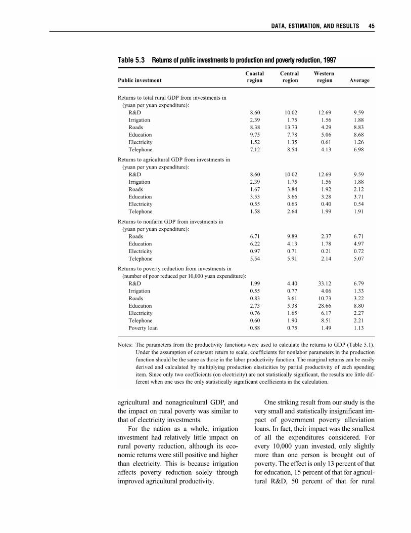
DATA, ESTIMATION, AND RESULTS 45
agricultural and nonagricultural GDP, and
the impact on rural poverty was similar to
that of electricity investments.
For the nation as a whole, irrigation
investment had relatively little impact on
rural poverty reduction, although its eco-
nomic returns were still positive and higher
than electricity. This is because irrigation
affects poverty reduction solely through
improved agricultural productivity.
One striking result from our study is the
very small and statistically insignificant im-
pact of government poverty alleviation
loans. In fact, their impact was the smallest
of all the expenditures considered. For
every 10,000 yuan invested, only slightly
more than one person is brought out of
poverty. The effect is only 13 percent of that
for education, 15 percent of that for agricul-
tural R&D, 50 percent of that for rural
Table 5.3 Returns of public investments to production and poverty reduction, 1997
Coastal Central Western
Public investment region region region Average
Returns to total rural GDP from investments in
(yuan per yuan expenditure):
R&D 8.60 10.02 12.69 9.59
Irrigation 2.39 1.75 1.56 1.88
Roads 8.38 13.73 4.29 8.83
Education 9.75 7.78 5.06 8.68
Electricity 1.52 1.35 0.61 1.26
Telephone 7.12 8.54 4.13 6.98
Returns to agricultural GDP from investments in
(yuan per yuan expenditure):
R&D 8.60 10.02 12.69 9.59
Irrigation 2.39 1.75 1.56 1.88
Roads 1.67 3.84 1.92 2.12
Education 3.53 3.66 3.28 3.71
Electricity 0.55 0.63 0.40 0.54
Telephone 1.58 2.64 1.99 1.91
Returns to nonfarm GDP from investments in
(yuan per yuan expenditure):
Roads 6.71 9.89 2.37 6.71
Education 6.22 4.13 1.78 4.97
Electricity 0.97 0.71 0.21 0.72
Telephone 5.54 5.91 2.14 5.07
Returns to poverty reduction from investments in
(number of poor reduced per 10,000 yuan expenditure):
R&D 1.99 4.40 33.12 6.79
Irrigation 0.55 0.77 4.06 1.33
Roads 0.83 3.61 10.73 3.22
Education 2.73 5.38 28.66 8.80
Electricity 0.76 1.65 6.17 2.27
Telephone 0.60 1.90 8.51 2.21
Poverty loan 0.88 0.75 1.49 1.13
Notes: The parameters from the productivity functions were used to calculate the returns to GDP (Table 5.1).
Under the assumption of constant return to scale, coefficients for nonlabor parameters in the production
function should be the same as those in the labor productivity function. The marginal returns can be easily
derived and calculated by multiplying production elasticities by partial productivity of each spending
item. Since only two coefficients (on electricity) are not statistically significant, the results are little dif-
ferent when one uses the only statistically significant coefficients in the calculation.
infrastructure, and is even smaller than that
for irrigation.
Regional variation is large in the mar-
ginal returns to government spending in
both GDP growth and poverty reduction.
In terms of poverty-reduction effects, all
kinds of investments had high returns in
the western region. For example, for every
10,000 yuan invested in agricultural R&D,
education, roads, telecommunications, and
electricity, the respective number of poor
reduced were 33, 29, 11, 9, and 6. These
effects are 4.8, 3.3, 3.2, 3.9, and 2.8 times
higher than the national average. Even for
irrigation, every 10,000 yuan additional
investment was sufficient to bring four
people out of poverty, three times higher
than the national average.
With respect to returns to growth in
agriculture, R&D investment had the high-
est return in the western region, while
irrigation investment had the highest return
in the coastal region. For education and
rural infrastructure (roads, electricity, and
telecommunications), the central region had
the highest returns. In the coastal region, a
large amount of land has been converted for
nonagricultural use due to rapid industrial-
ization and urbanization. Moreover, incen-
tives to intensify farming are lower there
because of more nonfarm employment
opportunities. In contrast, land in the west-
ern region is more marginal with limited
water and soil of low quality. Therefore,
major growth potential for agricultural pro-
duction lies in the central region, where
land is relatively less scarce and agricul-
tural production is still the main source of
farmers’ income.
Not surprisingly, most government ex-
penditures had their largest impact on rural
nonfarm GDP in the coastal and central areas.
Contributions to RegionalInequalityGiven the estimated coefficients for equa-
tions (2) and (3), we are in position to apply
the inequality decomposition method out-
lined in equations (17) and (18). Table 5.4
reports the contributions of each factor
to agricultural, nonagricultural, and total
labor productivities, respectively, for se-
lected years.
It is clear from Table 5.4 that regional
inequality in agricultural labor productivity
has not changed much. But the contribu-
tions of various inputs to the inequality
have changed dramatically. The contribu-
tions of three conventional inputs (capital,
labor, and land) declined, while the contri-
butions of most public investments, espe-
cially R&D, electrification, and telephones,
increased. Public investment’s total contri-
bution increased from 0.110 to 0.221 in
the study period.
In contrast to agricultural productivity,
regional inequality in nonagricultural labor
productivity almost doubled. Capital and
labor contributed little to worsening in-
equality, with public investment in electric-
ity, telephones, and in total the dominant
factor. Public investment’s contribution to
regional inequality in nonagricultural labor
productivity increased by 118 percent from
0.144 to 0.305 during the period.
In order to evaluate the effects of these
input factors on overall inequality, we sub-
stitute the log variance of agricultural labor
productivity and nonagricultural labor pro-
ductivity into equation (18). Using the esti-
mated parameters and the decomposition
method, we obtain the contributions of var-
ious input factors to overall inequality. Cap-
ital’s contribution to worsening regional
inequality increased from 0.085 to 0.220,
although its shares in the inequality of agri-
cultural and nonagricultural labor produc-
tivity changed little. This is probably due to
a structural shift in capital from agricultural
to nonagricultural production in the econ-
omy because rural industry is more capital
intensive than agriculture. For the same rea-
son, land and land-enhancing technologies,
especially irrigation, which are mainly used
in agricultural production, accounted for a
decreasing share of overall inequality. The
contributions of roads, agricultural R&D,
electricity, and telecommunications in-
46 CHAPTER 5
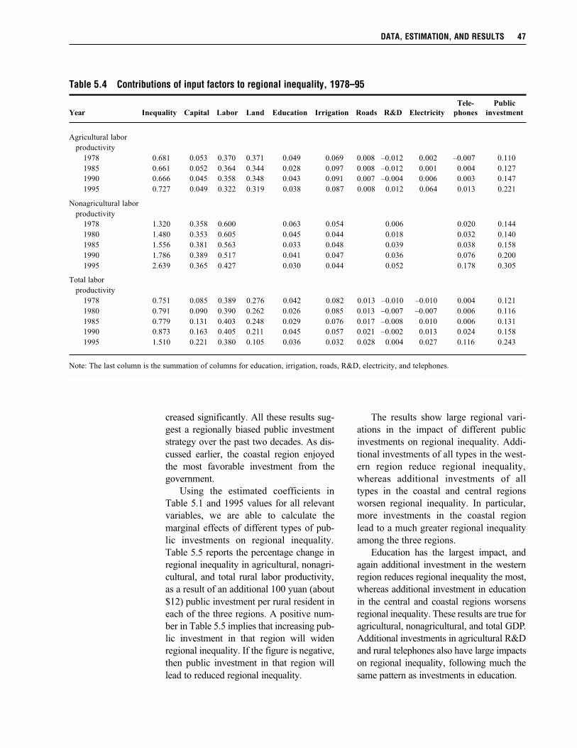
DATA, ESTIMATION, AND RESULTS 47
creased significantly. All these results sug-
gest a regionally biased public investment
strategy over the past two decades. As dis-
cussed earlier, the coastal region enjoyed
the most favorable investment from the
government.
Using the estimated coefficients in
Table 5.1 and 1995 values for all relevant
variables, we are able to calculate the
marginal effects of different types of pub-
lic investments on regional inequality.
Table 5.5 reports the percentage change in
regional inequality in agricultural, nonagri-
cultural, and total rural labor productivity,
as a result of an additional 100 yuan (about
$12) public investment per rural resident in
each of the three regions. A positive num-
ber in Table 5.5 implies that increasing pub-
lic investment in that region will widen
regional inequality. If the figure is negative,
then public investment in that region will
lead to reduced regional inequality.
The results show large regional vari-
ations in the impact of different public
investments on regional inequality. Addi-
tional investments of all types in the west-
ern region reduce regional inequality,
whereas additional investments of all
types in the coastal and central regions
worsen regional inequality. In particular,
more investments in the coastal region
lead to a much greater regional inequality
among the three regions.
Education has the largest impact, and
again additional investment in the western
region reduces regional inequality the most,
whereas additional investment in education
in the central and coastal regions worsens
regional inequality. These results are true for
agricultural, nonagricultural, and total GDP.
Additional investments in agricultural R&D
and rural telephones also have large impacts
on regional inequality, following much the
same pattern as investments in education.
Table 5.4 Contributions of input factors to regional inequality, 1978–95
Tele- Public
Year Inequality Capital Labor Land Education Irrigation Roads R&D Electricity phones investment
Agricultural labor
productivity
1978 0.681 0.053 0.370 0.371 0.049 0.069 0.008 –0.012 0.002 –0.007 0.110
1985 0.661 0.052 0.364 0.344 0.028 0.097 0.008 –0.012 0.001 0.004 0.127
1990 0.666 0.045 0.358 0.348 0.043 0.091 0.007 –0.004 0.006 0.003 0.147
1995 0.727 0.049 0.322 0.319 0.038 0.087 0.008 0.012 0.064 0.013 0.221
Nonagricultural labor
productivity
1978 1.320 0.358 0.600 0.063 0.054 0.006 0.020 0.144
1980 1.480 0.353 0.605 0.045 0.044 0.018 0.032 0.140
1985 1.556 0.381 0.563 0.033 0.048 0.039 0.038 0.158
1990 1.786 0.389 0.517 0.041 0.047 0.036 0.076 0.200
1995 2.639 0.365 0.427 0.030 0.044 0.052 0.178 0.305
Total labor
productivity
1978 0.751 0.085 0.389 0.276 0.042 0.082 0.013 –0.010 –0.010 0.004 0.121
1980 0.791 0.090 0.390 0.262 0.026 0.085 0.013 –0.007 –0.007 0.006 0.116
1985 0.779 0.131 0.403 0.248 0.029 0.076 0.017 –0.008 0.010 0.006 0.131
1990 0.873 0.163 0.405 0.211 0.045 0.057 0.021 –0.002 0.013 0.024 0.158
1995 1.510 0.221 0.380 0.105 0.036 0.032 0.028 0.004 0.027 0.116 0.243
Note: The last column is the summation of columns for education, irrigation, roads, R&D, electricity, and telephones.
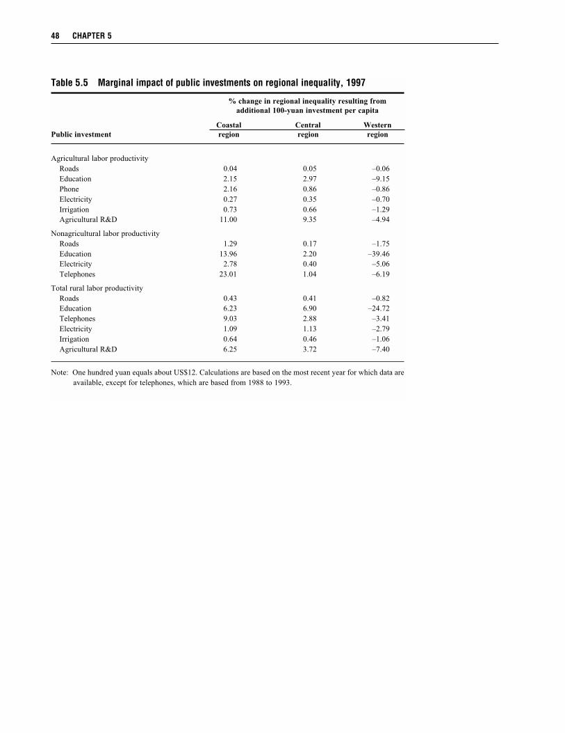
48 CHAPTER 5
Table 5.5 Marginal impact of public investments on regional inequality, 1997
% change in regional inequality resulting from
additional 100-yuan investment per capita
Coastal Central Western
Public investment region region region
Agricultural labor productivity
Roads 0.04 0.05 –0.06
Education 2.15 2.97 –9.15
Phone 2.16 0.86 –0.86
Electricity 0.27 0.35 –0.70
Irrigation 0.73 0.66 –1.29
Agricultural R&D 11.00 9.35 –4.94
Nonagricultural labor productivity
Roads 1.29 0.17 –1.75
Education 13.96 2.20 –39.46
Electricity 2.78 0.40 –5.06
Telephones 23.01 1.04 –6.19
Total rural labor productivity
Roads 0.43 0.41 –0.82
Education 6.23 6.90 –24.72
Telephones 9.03 2.88 –3.41
Electricity 1.09 1.13 –2.79
Irrigation 0.64 0.46 –1.06
Agricultural R&D 6.25 3.72 –7.40
Note: One hundred yuan equals about US$12. Calculations are based on the most recent year for which data are
available, except for telephones, which are based from 1988 to 1993.
C H A P T E R 6
Conclusions
T his chapter concludes our study by reporting major findings. It then highlights impli-
cations for future government investment priorities, points out future research direc-
tions, and draws lessons for other developing countries.
Major Findings
Using provincial-level data for 1970–97, this study developed a simultaneous equations model
to estimate the effects of different types of government expenditure on growth, regional
inequality, and rural poverty in China. The results show that government spending on pro-
duction-enhancing investments, such as agricultural research and development (R&D) and
irrigation, rural education, and infrastructure (including roads, electricity, and telecommuni-
cations) all contributed to agricultural productivity growth and reduced regional inequality and
rural poverty. But variations in their marginal effects on productivity were large, among the
different types of spending as well as across regions.
Government expenditure on education had the largest impact on poverty reduction and
very high returns to growth in agriculture and the nonfarm sector, as well as to the rural econ-
omy as a whole. Among all types of investments, additional spending on education in the less-
developed areas (the western region) also had the largest role in reducing regional inequality.
Government spending on agricultural research and extension improved agricultural pro-
duction substantially. In fact, this type of expenditure had the largest returns to growth in agri-
cultural production and overall in the rural economy. Since China is a large country, growth in
agriculture is still much needed to meet the increasing food needs of its richer and larger pop-
ulation. Agricultural growth also trickled down in large benefits for the rural poor. The impact
of R&D on poverty ranked second only to education investments.
Government spending on rural telecommunications, electricity, and roads also had substan-
tial marginal impact on rural poverty reduction. These poverty-reduction effects came mainly
from improved nonfarm employment and increased rural wages. Specifically, road investment
had the largest return to gross domestic product (GDP) growth in the nonfarm economy and the
second largest return to the overall rural economy, only slightly lower than R&D investment.
Irrigation investment had only modest impact on growth in agricultural production and
even less impact on rural poverty reduction, even after trickle-down benefits were allowed
for. This is consistent with the results of Fan, Hazell, and Thorat (1999) for India. Another
striking result is that government spending on loans specifically targeted for poverty allevi-
ation had the least impact on rural poverty reduction. Neither did this type of spending
have any obvious productivity effect. Again this is consistent with the Indian findings of
Fan, Hazell, and Thorat.
49
Additional investments in the western
region contribute most to reducing poverty
and regional inequality, because this is where
most of the poor are now concentrated. The
poverty-reduction effect of spending in
education, agricultural R&D, and roads is
especially high in the region. However,
economic returns to most investments are
larger in the central region. Fortunately the
trade-off between poverty reduction in the
western region and production increases in
the central region is rather small.
Priorities of FutureGovernment Investment
The results of this study have important pol-
icy implications for future priorities in gov-
ernment expenditure. As Table 3.1 showed,
rural education spending accounted for
41 percent of total expenditures in rural
areas in 1997. Irrigation is next, accounting
for 23 percent. The irrigation spending con-
sidered in this study was only that directly
related to irrigation, not including urban
water supply, navigation, and hydropower
generation. If the latter is included, the
spending easily doubles. Investment in rural
infrastructure took about 33 percent of total
government spending in rural areas, with
14 percent for rural power, 10 percent for
rural roads, and 9 percent for rural telecom-
munications. Agricultural research accounted
for only a small fraction of total government
investment in rural areas, at 2.2 percent.
Are these allocations optimal for maxi-
mized growth and poverty reduction and
balanced regional development? This study
reveals large differential impacts of various
types of government spending on growth,
poverty reduction, and regional inequality.
Potential gains from reallocating govern-
ment resources are enormous. Based on the
results of our study, we offer the following
policy suggestions:
1. The government should continue
efforts to increase its overall investment
in rural areas. Rural investment accounted
for only 19 percent of total government
expenditures in 1997, but rural residents
account for 69 percent of China’s total pop-
ulation. Moreover, almost 50 percent of
national GDP was produced by the rural
sector (agriculture and rural township and
village enterprises) in 1997. Government’s
rural spending as a percentage of rural GDP
is only about 5 percent compared with
11.6 percent for the whole economy. China
has implemented an urban- and industry-
biased investment policy for the past sev-
eral decades. As a result, the rural-urban
income gap is gigantic and has increased
over time. Any policies against the rural
sector will aggravate the existing disparity
and should be discontinued.
2. There is an urgent need to increase
investment in agricultural R&D. Agricul-
tural research expenditure as percentage of
agricultural gross domestic product AgGDP
is only 0.3 percent. This is extremely low in
comparison to the 2 percent spent in many
developed countries; it is even lower than in
most developing countries (0.5 percent).
Various evidence, including this study,
shows that agricultural research investment
not only has high economic returns (Fan
2000), but it also has a large impact in
reducing rural poverty and regional inequal-
ity. Moreover, new evidence has revealed
that agricultural research contributes to a
large drop in urban poverty through low-
ered food prices (Fan, Fang, and Zhang
2001). Without agricultural research, China
would have many more urban poor today.
Finally, increased agricultural research
investment is one of the most efficient ways
to solve China’s long-term food-security
problem (Huang, Rosegrant, and Rozelle
1999). All this suggests that increased in-
vestment in agricultural research is a “win-
win-win” (growth, poverty and equity, food
security) national development strategy.
3. The government should gear up its
investment in rural education, even though
its current rural education spending is al-
ready the largest of all rural expenditures.
Improved education helps farmers gain ac-
cess to and use new technologies generated
50 CHAPTER 6
by the research system, thereby promoting
agricultural growth. But more importantly,
education helps farmers to gain and im-
prove the skills they need for nonfarm jobs
in rural enterprises and for migration to the
urban sector. Our results show that rural ed-
ucation investment has the largest poverty-
reduction effect per unit of spending. There-
fore, continued increases in rural education
investment, particularly in the less-developed
western region, are a very effective means
of promoting growth in agriculture and rural
nonfarm employment and reducing rural
poverty and regional inequality.
4. Rural infrastructure should receive
high priority in government’s investment
portfolio. Like rural education, investments
in infrastructure contribute to reduce rural
poverty and regional inequality mainly by
spurring nonfarm employment and growth
in agricultural production. Among all rural
infrastructures, roads should receive special
attention, as they have the largest poverty-
reduction and growth impact (compared
with telecommunications and electricity).
5. China invested heavily in irrigation
in the past. Large-scale irrigation facilities
were built, and a high percentage of the
country’s arable land is now under irri-
gation. The marginal returns from further
investment may therefore be small and
declining, and future investments should
be geared to improving the efficiency of
existing public irrigation systems.
6. The low returns of rural poverty alle-
viation loans to poverty reduction indicate
that these loans should be better targeted.
Studies show that a large part of the funds
have gone to the nonpoor regions and to
nonpoor households, and many rural poor
do not benefit from them at all. The funds
are also often used for purposes such as
covering administrative costs of local gov-
ernments instead of for poverty alleviation.
Although government has realized the seri-
ousness of the problem, more efforts are
needed to better target the funds to the poor,
or otherwise use the moneys to improve
rural education and infrastructure, which
promote long-term growth and thereby offer
a long-term solution to poverty reduction.
7. The highest returns in the western re-
gion to all kinds of investment in reducing
both rural poverty and regional inequality,
as evidenced in this study, are consistent
with the national strategy to develop the
western region. In particular, investment in
agricultural research, education, and rural
infrastructure there should be the govern-
ment’s top priority. Considering China’s
decentralized fiscal system and the western
region’s small tax base, fiscal transfers from
the richer coastal region are called for to
develop the vast west.
Future Research Directions
A number of issues deserve more attention
in future research. First, China is on the
brink of joining the World Trade Organi-
zation (WTO). It is unclear how the gov-
ernment can use public investment as an
instrument to alleviate any negative effects
of WTO membership on national food
security and the welfare of the rural pop-
ulation. In particular, the poor in less-
developed areas such as the Northwest and
Southwest will suffer disproportionately,
because they are most sensitive to changes
in agricultural prices.
Second, a general-equilibrium analysis
is needed to analyze how government
investment in rural areas affects not only
the agricultural sector and rural areas, but
also other sectors and cities. Studies that
ignore these impacts severely under-
estimate the overall impact of public
investment on poverty.
Finally, an analysis of the political and
institutional context of public investments
and conditions for efficient provision of
public goods and services is also much
needed to improve the efficiency of public
investments. In particular, how the govern-
ment can design a mechanism (policies,
regulations, fiscal systems) to mobilize
public resources to invest in rural areas de-
serves more research attention in the future.
CONCLUSIONS 51
52 CHAPTER 6
How to reform public institutions by im-
proving the incentive system, account-
ability, human capital, and management
is also an important research issue.
Implications for OtherDeveloping Countries
The results of this study provide important
insights for other developing countries that
are redesigning their spending policy to
achieve development goals. Many devel-
oping countries are undergoing substan-
tial macroeconomic adjustments. It is un-
clear whether such programs will affect
government expenditures, and therefore
growth in agricultural production and re-
ductions in poverty.
Various empirical studies confirm the
important role of government spending in
spurring long-term growth in the national
economy (Tanzi and Zee 1997; Barro
1990) and in agriculture (Elias 1985; Fan,
Hazell, and Thorat 1999; Fan and Pardey
1997). But equally important to discern is
that different types of spending (for exam-
ple, by sector and by region) may have dif-
ferent impacts on growth, as shown in this
report. Moreover, different types of spend-
ing may have different implications for the
distribution of economic gains. Most im-
portantly, differing types of government
spending may result in different conse-
quences for the poor. Ways to alleviate
poverty are being increasingly debated
among academicians and policymakers.
Less known is how recent changes in the
level and composition of government ex-
penditures have affected growth and
poverty reduction in developing countries.
Since significant increases in public
rural investment seem unlikely, countries
will have to give greater emphasis to using
their public investment resources more
efficiently. This requires better targeting of
investment to achieve growth and poverty
alleviation goals and improved efficiency
within the agencies that provide public
goods and services. Reliable information
on the marginal effects of various types
of government spending is crucial for
government to make sound investment
decisions. Without such information, it is
difficult for governments to hone future
investment priorities to achieve national
development goals. There is therefore an
urgent need to conduct studies similar to
this one in other developing countries.
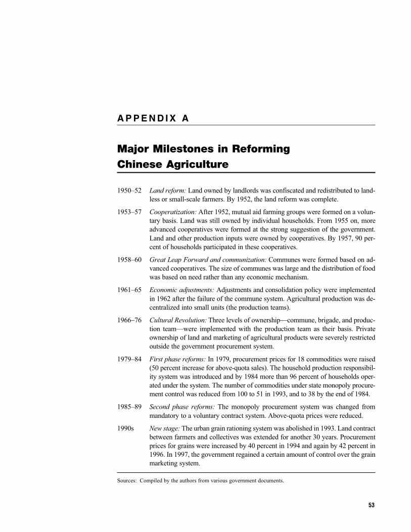
A P P E N D I X A
Major Milestones in ReformingChinese Agriculture
1950–52 Land reform: Land owned by landlords was confiscated and redistributed to land-
less or small-scale farmers. By 1952, the land reform was complete.
1953–57 Cooperatization: After 1952, mutual aid farming groups were formed on a volun-
tary basis. Land was still owned by individual households. From 1955 on, more
advanced cooperatives were formed at the strong suggestion of the government.
Land and other production inputs were owned by cooperatives. By 1957, 90 per-
cent of households participated in these cooperatives.
1958–60 Great Leap Forward and communization: Communes were formed based on ad-
vanced cooperatives. The size of communes was large and the distribution of food
was based on need rather than any economic mechanism.
1961–65 Economic adjustments: Adjustments and consolidation policy were implemented
in 1962 after the failure of the commune system. Agricultural production was de-
centralized into small units (the production teams).
1966–76 Cultural Revolution: Three levels of ownership—commune, brigade, and produc-
tion team—were implemented with the production team as their basis. Private
ownership of land and marketing of agricultural products were severely restricted
outside the government procurement system.
1979–84 First phase reforms: In 1979, procurement prices for 18 commodities were raised
(50 percent increase for above-quota sales). The household production responsibil-
ity system was introduced and by 1984 more than 96 percent of households oper-
ated under the system. The number of commodities under state monopoly procure-
ment control was reduced from 100 to 51 in 1993, and to 38 by the end of 1984.
1985–89 Second phase reforms: The monopoly procurement system was changed from
mandatory to a voluntary contract system. Above-quota prices were reduced.
1990s New stage: The urban grain rationing system was abolished in 1993. Land contract
between farmers and collectives was extended for another 30 years. Procurement
prices for grains were increased by 40 percent in 1994 and again by 42 percent in
1996. In 1997, the government regained a certain amount of control over the grain
marketing system.
Sources: Compiled by the authors from various government documents.
53
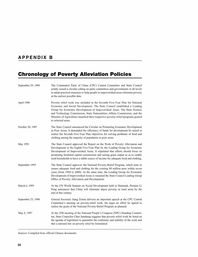
A P P E N D I X B
Chronology of Poverty Alleviation Policies
September 29, 1984 The Communist Party of China (CPC) Central Committee and State Council
jointly issued a circular calling on party committees and governments at all levels
to adopt practical measures to help people in impoverished areas eliminate poverty
at the earliest possible date.
April 1986 Poverty relief work was included in the Seventh Five-Year Plan for National
Economic and Social Development. The State Council established a Leading
Group for Economic Development of Impoverished Areas. The State Science
and Technology Commission, State Nationalities Affairs Commission, and the
Ministry of Agriculture launched their respective poverty-relief programs geared
to selected areas.
October 30, 1987 The State Council announced the Circular on Promoting Economic Development
in Poor Areas. It demanded the efficiency of funds for development be raised to
realize the Seventh Five-Year Plan objectives for solving problems of food and
clothing among the majority of population in poor areas.
May 1991 The State Council approved the Report on the Work of Poverty Alleviation and
Development in the Eighth Five-Year Plan by the Leading Group for Economic
Development of Impoverished Areas. It stipulated that efforts should focus on
promoting farmland capital construction and raising grain output so as to enable
rural households to have a stable source of income for adequate food and clothing.
September 1993 The State Council approves the National Poverty-Relief Program, which aims to
ensure adequate food and clothing for the existing 80 million poor within seven
years (from 1994 to 2000). At the same time, the Leading Group for Economic
Development of Impoverished Areas is renamed the State Council Leading Group
Office of Poverty Alleviation and Development.
March 6, 1995 At the UN World Summit on Social Development held in Denmark, Premier Li
Peng announces that China will eliminate abject poverty in rural areas by the
end of this century.
September 23, 1996 General Secretary Jiang Zemin delivers an important speech at the CPC Central
Committee’s meeting on poverty-relief work. He urges no effort be spared to
realize the goals of the National Poverty-Relief Program as planned.
May 6, 1997 At the 25th meeting of the National People’s Congress (NPC) Standing Commit-
tee, State Councilor Chen Junsheng suggests that poverty-relief work be listed on
the agenda of legislation to guarantee the continuity and stability of the work and
that a national law on poverty relief be formulated.
Sources: Compiled from official Chinese documents.
54
A P P E N D I X C
Provincial Data on Rural Public Spending
Sub-national-level data on public spending by various investment items are not easily
available for most developing countries. China is no exception in this, although these
data have become more accessible. Most such data are published in Chinese and must
be compiled from different sources. Moreover, the definitions, scope, and coverage of the
variables may vary over time and across regions (explained in detail in Chapter 5). For these
reasons, this appendix includes some of the recently released provincial data used in the
authors’ analysis, which might be of more general interest.
All spending data were deflated into 1990 prices using the GDP deflator unless specified
otherwise. Income data was deflated into 1990 prices using the consumer price index, while
agricultural output values and agricultural and nonagricultural GDP were measured in 1990
constant prices.
China has also experienced boundary changes over the last two decades. Hainan province
was created in 1987, having been part of Guangdong province prior to that. This analysis still
includes Hainan as part of Guangdong. Chongqing was created in 1997 out of Sichuan
province. For the 1997 data, Chongqing was thus aggregated into Sichuan province.
55
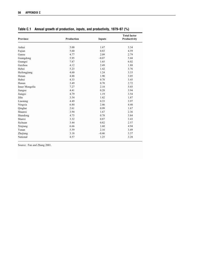
56 APPENDIX C
Table C.1 Annual growth of production, inputs, and productivity, 1979–97 (%)
Total factor
Province Production Inputs Productivity
Anhui 5.00 1.67 3.34
Fujian 5.60 0.83 4.59
Gansu 4.77 2.09 2.79
Guangdong 5.95 –0.07 5.68
Guangxi 7.87 1.65 6.02
Guizhou 4.12 2.49 1.88
Hebei 5.23 1.42 3.76
Heilongjiang 4.60 1.24 3.33
Henan 4.88 1.90 3.05
Hubei 4.33 0.78 3.45
Hunan 3.49 0.70 2.72
Inner Mongolia 7.27 2.18 5.03
Jiangsu 4.41 0.28 3.94
Jiangxi 4.79 1.19 3.54
Jilin 3.54 1.82 1.87
Liaoning 4.49 0.33 3.97
Ningxia 6.84 2.46 4.40
Qinghai 2.61 0.99 1.67
Shaanxi 3.94 1.67 2.36
Shandong 4.75 0.78 3.84
Shanxi 3.32 0.87 2.43
Sichuan 3.44 0.82 2.57
Xinjiang 6.66 1.60 4.94
Yunan 5.59 2.16 3.49
Zhejiang 3.18 –0.46 3.37
National 4.57 1.25 3.28
Source: Fan and Zhang 2001.
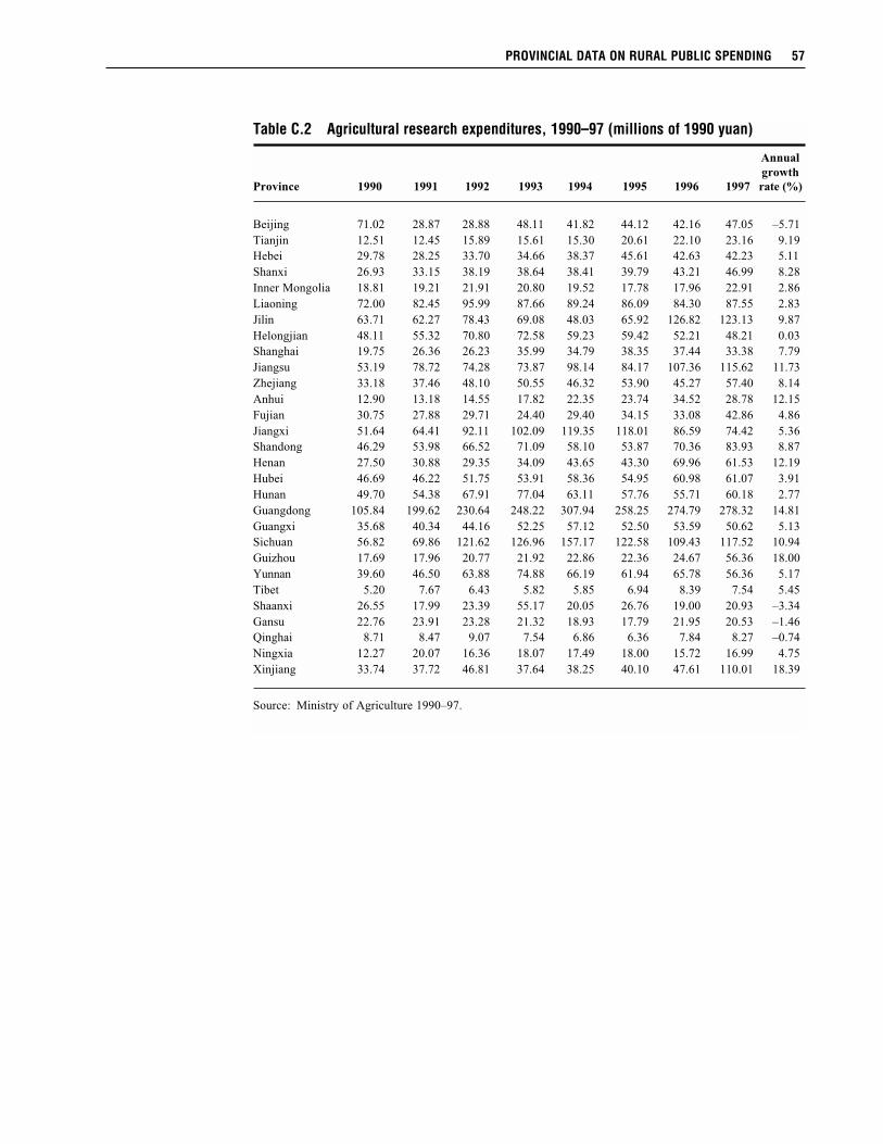
PROVINCIAL DATA ON RURAL PUBLIC SPENDING 57
Table C.2 Agricultural research expenditures, 1990–97 (millions of 1990 yuan)
Annual
growth
Province 1990 1991 1992 1993 1994 1995 1996 1997 rate (%)
Beijing 71.02 28.87 28.88 48.11 41.82 44.12 42.16 47.05 –5.71
Tianjin 12.51 12.45 15.89 15.61 15.30 20.61 22.10 23.16 9.19
Hebei 29.78 28.25 33.70 34.66 38.37 45.61 42.63 42.23 5.11
Shanxi 26.93 33.15 38.19 38.64 38.41 39.79 43.21 46.99 8.28
Inner Mongolia 18.81 19.21 21.91 20.80 19.52 17.78 17.96 22.91 2.86
Liaoning 72.00 82.45 95.99 87.66 89.24 86.09 84.30 87.55 2.83
Jilin 63.71 62.27 78.43 69.08 48.03 65.92 126.82 123.13 9.87
Helongjian 48.11 55.32 70.80 72.58 59.23 59.42 52.21 48.21 0.03
Shanghai 19.75 26.36 26.23 35.99 34.79 38.35 37.44 33.38 7.79
Jiangsu 53.19 78.72 74.28 73.87 98.14 84.17 107.36 115.62 11.73
Zhejiang 33.18 37.46 48.10 50.55 46.32 53.90 45.27 57.40 8.14
Anhui 12.90 13.18 14.55 17.82 22.35 23.74 34.52 28.78 12.15
Fujian 30.75 27.88 29.71 24.40 29.40 34.15 33.08 42.86 4.86
Jiangxi 51.64 64.41 92.11 102.09 119.35 118.01 86.59 74.42 5.36
Shandong 46.29 53.98 66.52 71.09 58.10 53.87 70.36 83.93 8.87
Henan 27.50 30.88 29.35 34.09 43.65 43.30 69.96 61.53 12.19
Hubei 46.69 46.22 51.75 53.91 58.36 54.95 60.98 61.07 3.91
Hunan 49.70 54.38 67.91 77.04 63.11 57.76 55.71 60.18 2.77
Guangdong 105.84 199.62 230.64 248.22 307.94 258.25 274.79 278.32 14.81
Guangxi 35.68 40.34 44.16 52.25 57.12 52.50 53.59 50.62 5.13
Sichuan 56.82 69.86 121.62 126.96 157.17 122.58 109.43 117.52 10.94
Guizhou 17.69 17.96 20.77 21.92 22.86 22.36 24.67 56.36 18.00
Yunnan 39.60 46.50 63.88 74.88 66.19 61.94 65.78 56.36 5.17
Tibet 5.20 7.67 6.43 5.82 5.85 6.94 8.39 7.54 5.45
Shaanxi 26.55 17.99 23.39 55.17 20.05 26.76 19.00 20.93 –3.34
Gansu 22.76 23.91 23.28 21.32 18.93 17.79 21.95 20.53 –1.46
Qinghai 8.71 8.47 9.07 7.54 6.86 6.36 7.84 8.27 –0.74
Ningxia 12.27 20.07 16.36 18.07 17.49 18.00 15.72 16.99 4.75
Xinjiang 33.74 37.72 46.81 37.64 38.25 40.10 47.61 110.01 18.39
Source: Ministry of Agriculture 1990–97.
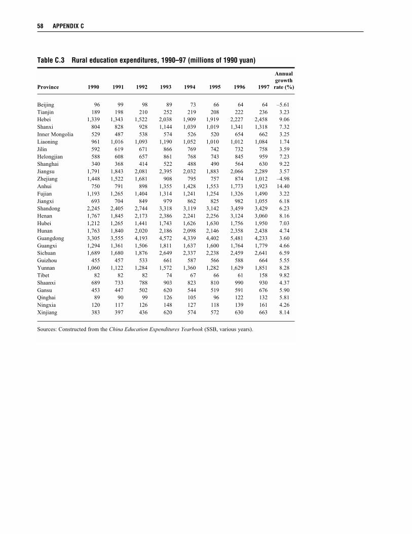
58 APPENDIX C
Table C.3 Rural education expenditures, 1990–97 (millions of 1990 yuan)
Annual
growth
Province 1990 1991 1992 1993 1994 1995 1996 1997 rate (%)
Beijing 96 99 98 89 73 66 64 64 –5.61
Tianjin 189 198 210 252 219 208 222 236 3.23
Hebei 1,339 1,343 1,522 2,038 1,909 1,919 2,227 2,458 9.06
Shanxi 804 828 928 1,144 1,039 1,019 1,341 1,318 7.32
Inner Mongolia 529 487 538 574 526 520 654 662 3.25
Liaoning 961 1,016 1,093 1,190 1,052 1,010 1,012 1,084 1.74
Jilin 592 619 671 866 769 742 732 758 3.59
Helongjian 588 608 657 861 768 743 845 959 7.23
Shanghai 340 368 414 522 488 490 564 630 9.22
Jiangsu 1,791 1,843 2,081 2,395 2,032 1,883 2,066 2,289 3.57
Zhejiang 1,448 1,522 1,681 908 795 757 874 1,012 –4.98
Anhui 750 791 898 1,355 1,428 1,553 1,773 1,923 14.40
Fujian 1,193 1,265 1,404 1,314 1,241 1,254 1,326 1,490 3.22
Jiangxi 693 704 849 979 862 825 982 1,055 6.18
Shandong 2,245 2,405 2,744 3,318 3,119 3,142 3,459 3,429 6.23
Henan 1,767 1,845 2,173 2,386 2,241 2,256 3,124 3,060 8.16
Hubei 1,212 1,265 1,441 1,743 1,626 1,630 1,756 1,950 7.03
Hunan 1,763 1,840 2,020 2,186 2,098 2,146 2,358 2,438 4.74
Guangdong 3,305 3,555 4,193 4,572 4,339 4,402 5,481 4,233 3.60
Guangxi 1,294 1,361 1,506 1,811 1,637 1,600 1,764 1,779 4.66
Sichuan 1,689 1,680 1,876 2,649 2,337 2,238 2,459 2,641 6.59
Guizhou 455 457 533 661 587 566 588 664 5.55
Yunnan 1,060 1,122 1,284 1,572 1,360 1,282 1,629 1,851 8.28
Tibet 82 82 82 74 67 66 61 158 9.82
Shaanxi 689 733 788 903 823 810 990 930 4.37
Gansu 453 447 502 620 544 519 591 676 5.90
Qinghai 89 90 99 126 105 96 122 132 5.81
Ningxia 120 117 126 148 127 118 139 161 4.26
Xinjiang 383 397 436 620 574 572 630 663 8.14
Sources: Constructed from the China Education Expenditures Yearbook (SSB, various years).
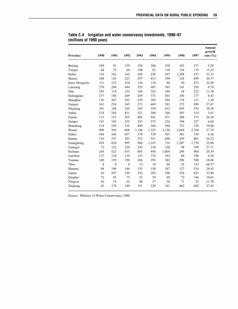
PROVINCIAL DATA ON RURAL PUBLIC SPENDING 59
Table C.4 Irrigation and water conservancy investments, 1990–97(millions of 1990 yuan)
Annual
growth
Province 1990 1991 1992 1993 1994 1995 1996 1997 rate (%)
Beijing 189 91 139 356 260 230 102 271 5.28
Tianjin 44 75 64 108 82 110 136 119 15.23
Hebei 110 102 162 204 228 297 1,204 473 23.15
Shanxi 108 136 223 297 413 396 128 699 30.57
Inner Mongolia 111 132 154 154 110 86 50 473 22.99
Liaoning 270 286 444 555 407 503 141 285 0.78
Jilin 105 119 153 168 165 186 34 223 11.38
Helongjian 157 188 269 269 373 303 106 277 8.43
Shanghai 136 207 293 359 383 204 174 151 1.50
Jiangsu 161 254 345 371 469 583 372 890 27.67
Zhejiang 101 168 265 265 359 412 695 976 38.28
Anhui 214 284 431 321 204 268 365 314 5.61
Fujian 113 153 263 402 441 471 208 573 26.10
Jiangxi 143 185 235 233 275 234 104 227 6.84
Shandong 214 258 525 489 564 504 731 726 19.06
Henan 498 569 868 1,146 1,325 2,120 2,684 2,764 27.74
Hubei 344 366 657 374 539 507 365 530 6.38
Hunan 156 197 385 552 551 690 439 801 26.32
Guangdong 438 824 995 960 1,147 716 1,207 1,770 22.08
Guangxi 72 152 220 245 310 320 98 399 27.71
Sichuan 264 523 655 865 894 1,004 296 968 20.39
Guizhou 127 128 139 152 155 163 60 198 6.54
Yunnan 149 159 198 268 293 382 296 500 18.88
Tibet 4 0 0 12 19 88 25 155 68.57
Shaanxi 94 109 144 155 150 187 127 554 28.83
Gansu 56 297 330 352 303 296 238 423 33.48
Qinghai 72 45 75 52 59 69 72 146 10.63
Ningxia 56 55 62 40 37 36 71 23 –11.70
Xinjiang 65 179 189 191 229 181 462 602 37.45
Source: Ministry of Water Conservancy 1980.
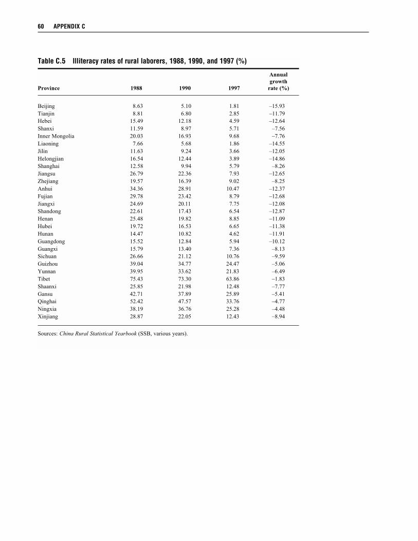
60 APPENDIX C
Table C.5 Illiteracy rates of rural laborers, 1988, 1990, and 1997 (%)
Annual
growth
Province 1988 1990 1997 rate (%)
Beijing 8.63 5.10 1.81 –15.93
Tianjin 8.81 6.80 2.85 –11.79
Hebei 15.49 12.18 4.59 –12.64
Shanxi 11.59 8.97 5.71 –7.56
Inner Mongolia 20.03 16.93 9.68 –7.76
Liaoning 7.66 5.68 1.86 –14.55
Jilin 11.63 9.24 3.66 –12.05
Helongjian 16.54 12.44 3.89 –14.86
Shanghai 12.58 9.94 5.79 –8.26
Jiangsu 26.79 22.36 7.93 –12.65
Zhejiang 19.57 16.39 9.02 –8.25
Anhui 34.36 28.91 10.47 –12.37
Fujian 29.78 23.42 8.79 –12.68
Jiangxi 24.69 20.11 7.75 –12.08
Shandong 22.61 17.43 6.54 –12.87
Henan 25.48 19.82 8.85 –11.09
Hubei 19.72 16.53 6.65 –11.38
Hunan 14.47 10.82 4.62 –11.91
Guangdong 15.52 12.84 5.94 –10.12
Guangxi 15.79 13.40 7.36 –8.13
Sichuan 26.66 21.12 10.76 –9.59
Guizhou 39.04 34.77 24.47 –5.06
Yunnan 39.95 33.62 21.83 –6.49
Tibet 75.43 73.30 63.86 –1.83
Shaanxi 25.85 21.98 12.48 –7.77
Gansu 42.71 37.89 25.89 –5.41
Qinghai 52.42 47.57 33.76 –4.77
Ningxia 38.19 36.76 25.28 –4.48
Xinjiang 28.87 22.05 12.43 –8.94
Sources: China Rural Statistical Yearbook (SSB, various years).
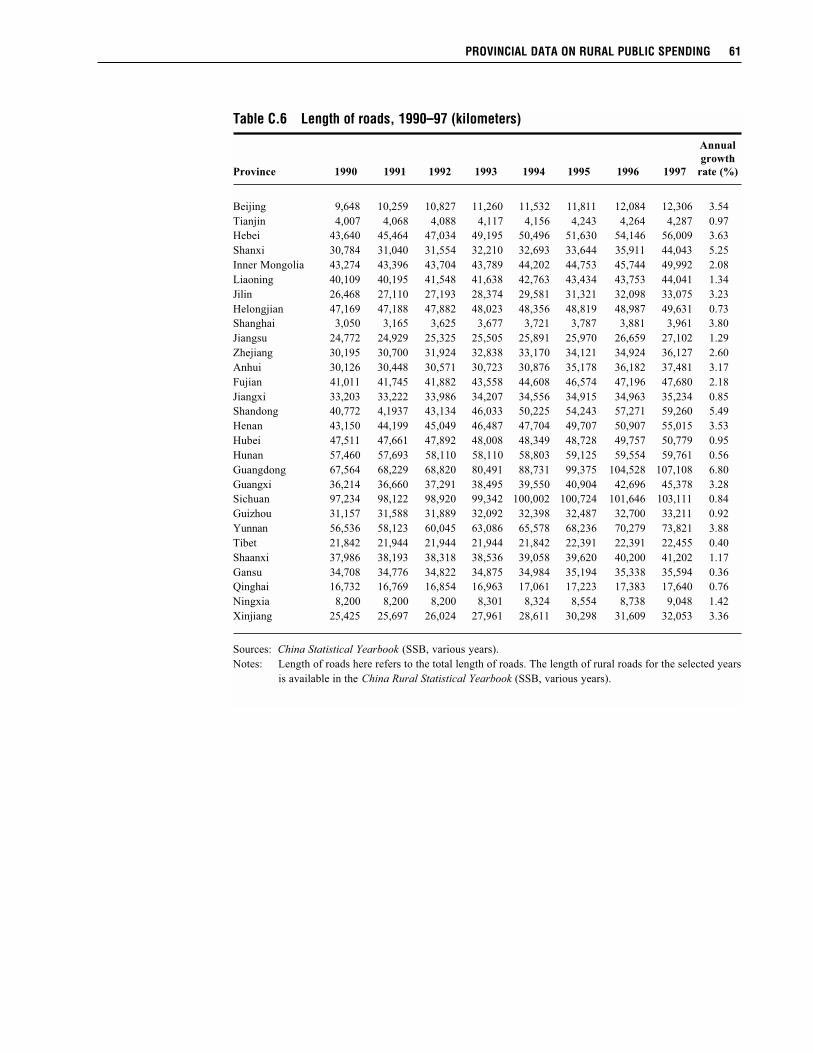
PROVINCIAL DATA ON RURAL PUBLIC SPENDING 61
Table C.6 Length of roads, 1990–97 (kilometers)
Annual
growth
Province 1990 1991 1992 1993 1994 1995 1996 1997 rate (%)
Beijing 9,648 10,259 10,827 11,260 11,532 11,811 12,084 12,306 3.54
Tianjin 4,007 4,068 4,088 4,117 4,156 4,243 4,264 4,287 0.97
Hebei 43,640 45,464 47,034 49,195 50,496 51,630 54,146 56,009 3.63
Shanxi 30,784 31,040 31,554 32,210 32,693 33,644 35,911 44,043 5.25
Inner Mongolia 43,274 43,396 43,704 43,789 44,202 44,753 45,744 49,992 2.08
Liaoning 40,109 40,195 41,548 41,638 42,763 43,434 43,753 44,041 1.34
Jilin 26,468 27,110 27,193 28,374 29,581 31,321 32,098 33,075 3.23
Helongjian 47,169 47,188 47,882 48,023 48,356 48,819 48,987 49,631 0.73
Shanghai 3,050 3,165 3,625 3,677 3,721 3,787 3,881 3,961 3.80
Jiangsu 24,772 24,929 25,325 25,505 25,891 25,970 26,659 27,102 1.29
Zhejiang 30,195 30,700 31,924 32,838 33,170 34,121 34,924 36,127 2.60
Anhui 30,126 30,448 30,571 30,723 30,876 35,178 36,182 37,481 3.17
Fujian 41,011 41,745 41,882 43,558 44,608 46,574 47,196 47,680 2.18
Jiangxi 33,203 33,222 33,986 34,207 34,556 34,915 34,963 35,234 0.85
Shandong 40,772 4,1937 43,134 46,033 50,225 54,243 57,271 59,260 5.49
Henan 43,150 44,199 45,049 46,487 47,704 49,707 50,907 55,015 3.53
Hubei 47,511 47,661 47,892 48,008 48,349 48,728 49,757 50,779 0.95
Hunan 57,460 57,693 58,110 58,110 58,803 59,125 59,554 59,761 0.56
Guangdong 67,564 68,229 68,820 80,491 88,731 99,375 104,528 107,108 6.80
Guangxi 36,214 36,660 37,291 38,495 39,550 40,904 42,696 45,378 3.28
Sichuan 97,234 98,122 98,920 99,342 100,002 100,724 101,646 103,111 0.84
Guizhou 31,157 31,588 31,889 32,092 32,398 32,487 32,700 33,211 0.92
Yunnan 56,536 58,123 60,045 63,086 65,578 68,236 70,279 73,821 3.88
Tibet 21,842 21,944 21,944 21,944 21,842 22,391 22,391 22,455 0.40
Shaanxi 37,986 38,193 38,318 38,536 39,058 39,620 40,200 41,202 1.17
Gansu 34,708 34,776 34,822 34,875 34,984 35,194 35,338 35,594 0.36
Qinghai 16,732 16,769 16,854 16,963 17,061 17,223 17,383 17,640 0.76
Ningxia 8,200 8,200 8,200 8,301 8,324 8,554 8,738 9,048 1.42
Xinjiang 25,425 25,697 26,024 27,961 28,611 30,298 31,609 32,053 3.36
Sources: China Statistical Yearbook (SSB, various years).
Notes: Length of roads here refers to the total length of roads. The length of rural roads for the selected years
is available in the China Rural Statistical Yearbook (SSB, various years).
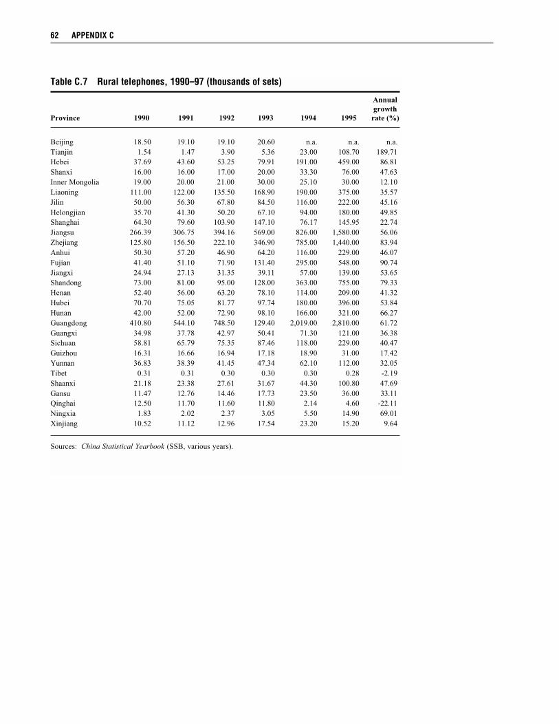
62 APPENDIX C
Table C.7 Rural telephones, 1990–97 (thousands of sets)
Annual
growth
Province 1990 1991 1992 1993 1994 1995 rate (%)
Beijing 18.50 19.10 19.10 20.60 n.a. n.a. n.a.
Tianjin 1.54 1.47 3.90 5.36 23.00 108.70 189.71
Hebei 37.69 43.60 53.25 79.91 191.00 459.00 86.81
Shanxi 16.00 16.00 17.00 20.00 33.30 76.00 47.63
Inner Mongolia 19.00 20.00 21.00 30.00 25.10 30.00 12.10
Liaoning 111.00 122.00 135.50 168.90 190.00 375.00 35.57
Jilin 50.00 56.30 67.80 84.50 116.00 222.00 45.16
Helongjian 35.70 41.30 50.20 67.10 94.00 180.00 49.85
Shanghai 64.30 79.60 103.90 147.10 76.17 145.95 22.74
Jiangsu 266.39 306.75 394.16 569.00 826.00 1,580.00 56.06
Zhejiang 125.80 156.50 222.10 346.90 785.00 1,440.00 83.94
Anhui 50.30 57.20 46.90 64.20 116.00 229.00 46.07
Fujian 41.40 51.10 71.90 131.40 295.00 548.00 90.74
Jiangxi 24.94 27.13 31.35 39.11 57.00 139.00 53.65
Shandong 73.00 81.00 95.00 128.00 363.00 755.00 79.33
Henan 52.40 56.00 63.20 78.10 114.00 209.00 41.32
Hubei 70.70 75.05 81.77 97.74 180.00 396.00 53.84
Hunan 42.00 52.00 72.90 98.10 166.00 321.00 66.27
Guangdong 410.80 544.10 748.50 129.40 2,019.00 2,810.00 61.72
Guangxi 34.98 37.78 42.97 50.41 71.30 121.00 36.38
Sichuan 58.81 65.79 75.35 87.46 118.00 229.00 40.47
Guizhou 16.31 16.66 16.94 17.18 18.90 31.00 17.42
Yunnan 36.83 38.39 41.45 47.34 62.10 112.00 32.05
Tibet 0.31 0.31 0.30 0.30 0.30 0.28 -2.19
Shaanxi 21.18 23.38 27.61 31.67 44.30 100.80 47.69
Gansu 11.47 12.76 14.46 17.73 23.50 36.00 33.11
Qinghai 12.50 11.70 11.60 11.80 2.14 4.60 -22.11
Ningxia 1.83 2.02 2.37 3.05 5.50 14.90 69.01
Xinjiang 10.52 11.12 12.96 17.54 23.20 15.20 9.64
Sources: China Statistical Yearbook (SSB, various years).
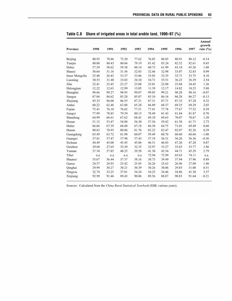
PROVINCIAL DATA ON RURAL PUBLIC SPENDING 63
Table C.8 Share of irrigated areas in total arable land, 1990–97 (%)
Annual
growth
Province 1990 1991 1992 1993 1994 1995 1996 1997 rate (%)
Beijing 80.93 78.86 75.20 77.62 76.85 80.85 80.91 80.12 –0.14
Tianjin 80.06 80.43 80.66 79.19 81.42 83.24 82.52 82.61 0.45
Hebei 57.29 58.62 59.38 60.14 60.73 61.99 65.18 65.26 1.88
Shanxi 30.64 31.16 31.56 32.03 32.46 32.98 33.07 32.83 0.99
Inner Mongolia 25.48 26.43 33.37 33.86 33.03 32.35 33.71 33.75 4.10
Liaoning 30.53 31.48 33.03 34.10 34.71 35.51 36.23 36.39 2.54
Jilin 22.41 23.45 23.27 23.08 23.01 22.88 23.68 24.45 1.26
Helongjian 12.22 12.63 12.99 13.05 11.39 12.17 14.82 18.23 5.88
Shanghai 98.66 99.27 98.93 99.07 99.05 99.21 98.28 98.16 –0.07
Jiangsu 87.04 84.62 85.28 85.07 85.10 86.16 86.28 86.27 –0.13
Zhejiang 85.33 86.08 86.55 87.21 87.31 87.71 87.32 87.28 0.32
Anhui 60.22 62.46 63.88 65.28 66.89 68.37 69.25 69.29 2.03
Fujian 75.41 76.10 76.82 77.51 77.41 77.78 77.67 77.52 0.39
Jiangxi 77.99 78.85 79.39 80.15 78.49 81.43 81.84 81.87 0.70
Shandong 64.99 66.61 67.62 68.41 69.10 69.63 70.07 70.67 1.20
Henan 51.12 53.47 54.88 56.30 57.56 59.42 61.58 61.71 2.73
Hubei 66.66 67.39 68.80 67.18 66.30 64.75 71.01 69.49 0.60
Hunan 80.63 78.93 80.86 81.76 82.22 82.47 82.07 82.26 0.29
Guangdong 65.49 63.72 61.98 60.07 59.49 60.76 60.60 60.68 –1.08
Guangxi 57.81 57.47 57.98 57.43 57.19 56.31 56.26 56.36 –0.36
Sichuan 44.49 45.00 45.45 45.86 46.31 46.83 47.26 47.28 0.87
Guizhou 29.68 27.65 33.39 32.35 32.97 33.27 33.63 33.77 1.86
Yunnan 37.34 37.85 40.25 39.58 41.30 43.54 44.71 45.29 2.79
Tibet n.a n.a n.a n.a 72.94 72.99 65.63 74.11 n.a.
Shaanxi 35.67 36.44 37.37 38.16 38.73 39.49 37.94 37.96 0.89
Gansu 24.57 24.93 25.42 25.85 26.26 25.63 26.96 27.09 1.40
Qinghai 29.99 30.27 30.21 30.39 30.26 30.06 29.85 31.08 0.51
Ningxia 32.74 33.25 37.01 34.24 34.25 34.46 34.86 41.30 3.37
Xinjiang 92.99 91.46 89.43 90.06 89.56 88.87 90.83 91.64 –0.21
Sources: Calculated from the China Rural Statistical Yearbook (SSB, various years).
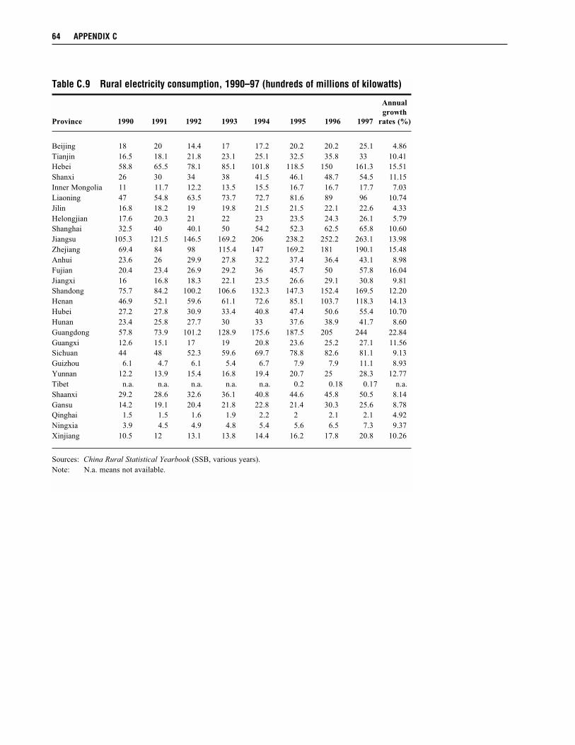
64 APPENDIX C
Table C.9 Rural electricity consumption, 1990–97 (hundreds of millions of kilowatts)
Annual
growth
Province 1990 1991 1992 1993 1994 1995 1996 1997 rates (%)
Beijing 18 20 14.4 17 17.2 20.2 20.2 25.1 4.86
Tianjin 16.5 18.1 21.8 23.1 25.1 32.5 35.8 33 10.41
Hebei 58.8 65.5 78.1 85.1 101.8 118.5 150 161.3 15.51
Shanxi 26 30 34 38 41.5 46.1 48.7 54.5 11.15
Inner Mongolia 11 11.7 12.2 13.5 15.5 16.7 16.7 17.7 7.03
Liaoning 47 54.8 63.5 73.7 72.7 81.6 89 96 10.74
Jilin 16.8 18.2 19 19.8 21.5 21.5 22.1 22.6 4.33
Helongjian 17.6 20.3 21 22 23 23.5 24.3 26.1 5.79
Shanghai 32.5 40 40.1 50 54.2 52.3 62.5 65.8 10.60
Jiangsu 105.3 121.5 146.5 169.2 206 238.2 252.2 263.1 13.98
Zhejiang 69.4 84 98 115.4 147 169.2 181 190.1 15.48
Anhui 23.6 26 29.9 27.8 32.2 37.4 36.4 43.1 8.98
Fujian 20.4 23.4 26.9 29.2 36 45.7 50 57.8 16.04
Jiangxi 16 16.8 18.3 22.1 23.5 26.6 29.1 30.8 9.81
Shandong 75.7 84.2 100.2 106.6 132.3 147.3 152.4 169.5 12.20
Henan 46.9 52.1 59.6 61.1 72.6 85.1 103.7 118.3 14.13
Hubei 27.2 27.8 30.9 33.4 40.8 47.4 50.6 55.4 10.70
Hunan 23.4 25.8 27.7 30 33 37.6 38.9 41.7 8.60
Guangdong 57.8 73.9 101.2 128.9 175.6 187.5 205 244 22.84
Guangxi 12.6 15.1 17 19 20.8 23.6 25.2 27.1 11.56
Sichuan 44 48 52.3 59.6 69.7 78.8 82.6 81.1 9.13
Guizhou 6.1 4.7 6.1 5.4 6.7 7.9 7.9 11.1 8.93
Yunnan 12.2 13.9 15.4 16.8 19.4 20.7 25 28.3 12.77
Tibet n.a. n.a. n.a. n.a. n.a. 0.2 0.18 0.17 n.a.
Shaanxi 29.2 28.6 32.6 36.1 40.8 44.6 45.8 50.5 8.14
Gansu 14.2 19.1 20.4 21.8 22.8 21.4 30.3 25.6 8.78
Qinghai 1.5 1.5 1.6 1.9 2.2 2 2.1 2.1 4.92
Ningxia 3.9 4.5 4.9 4.8 5.4 5.6 6.5 7.3 9.37
Xinjiang 10.5 12 13.1 13.8 14.4 16.2 17.8 20.8 10.26
Sources: China Rural Statistical Yearbook (SSB, various years).
Note: N.a. means not available.
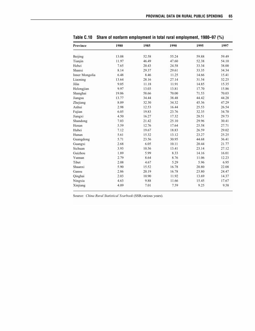
PROVINCIAL DATA ON RURAL PUBLIC SPENDING 65
Table C.10 Share of nonfarm employment in total rural employment, 1980–97 (%)
Province 1980 1985 1990 1995 1997
Beijing 13.08 52.58 55.24 59.88 59.49
Tianjin 11.97 46.49 47.60 52.38 54.10
Hebei 7.65 20.43 24.58 33.34 38.00
Shanxi 8.14 29.37 29.61 33.35 34.34
Inner Mongolia 6.48 8.46 11.25 14.66 15.41
Liaoning 13.64 28.16 27.14 31.54 32.25
Jilin 9.05 11.18 11.91 14.85 15.35
Helongjian 9.97 13.03 13.81 17.70 15.86
Shanghai 19.06 58.66 70.00 71.53 70.03
Jiangsu 13.77 34.44 38.48 44.42 44.28
Zhejiang 8.09 32.30 34.32 45.36 47.29
Anhui 2.98 12.53 16.44 25.53 26.54
Fujian 6.05 19.83 23.76 32.35 34.70
Jiangxi 4.50 16.27 17.32 28.51 29.73
Shandong 7.03 21.42 25.10 29.96 30.41
Henan 5.59 12.76 17.64 25.58 27.71
Hubei 7.12 19.67 18.83 26.59 29.02
Hunan 5.61 15.32 13.12 23.27 25.25
Guangdong 5.71 23.56 30.95 44.68 36.41
Guangxi 2.68 6.05 10.11 20.44 21.77
Sichuan 3.93 10.56 13.41 23.14 27.12
Guizhou 1.89 5.99 8.33 14.16 16.01
Yunnan 2.79 8.64 8.76 11.06 12.23
Tibet 2.08 4.67 5.29 5.96 6.95
Shaanxi 5.90 15.52 16.78 20.80 22.08
Gansu 2.86 20.19 16.78 23.80 24.47
Qinghai 2.03 10.90 11.92 13.69 14.37
Ningxia 4.63 9.88 11.66 15.45 17.67
Xinjiang 4.09 7.01 7.59 9.25 9.58
Source: China Rural Statistical Yearbook (SSB,various years).
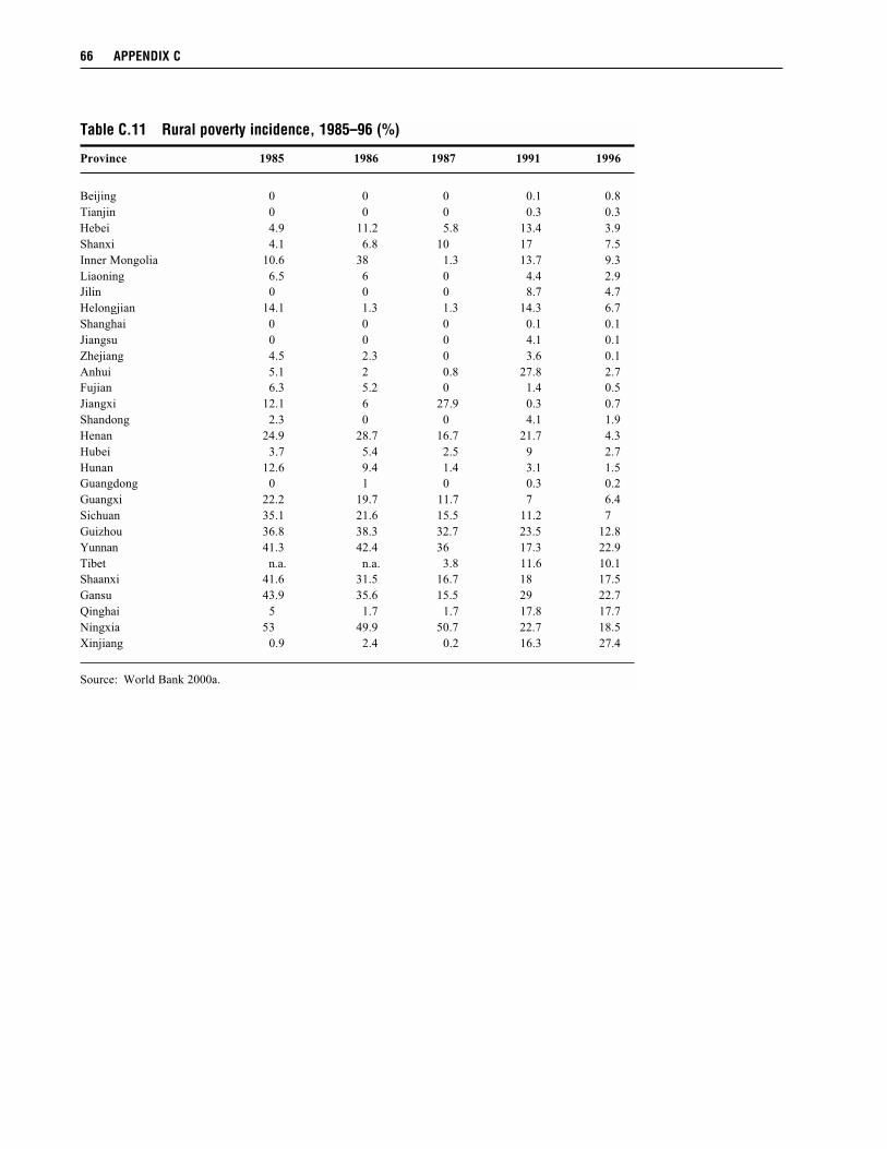
66 APPENDIX C
Table C.11 Rural poverty incidence, 1985–96 (%)
Province 1985 1986 1987 1991 1996
Beijing 0 0 0 0.1 0.8
Tianjin 0 0 0 0.3 0.3
Hebei 4.9 11.2 5.8 13.4 3.9
Shanxi 4.1 6.8 10 17 7.5
Inner Mongolia 10.6 38 1.3 13.7 9.3
Liaoning 6.5 6 0 4.4 2.9
Jilin 0 0 0 8.7 4.7
Helongjian 14.1 1.3 1.3 14.3 6.7
Shanghai 0 0 0 0.1 0.1
Jiangsu 0 0 0 4.1 0.1
Zhejiang 4.5 2.3 0 3.6 0.1
Anhui 5.1 2 0.8 27.8 2.7
Fujian 6.3 5.2 0 1.4 0.5
Jiangxi 12.1 6 27.9 0.3 0.7
Shandong 2.3 0 0 4.1 1.9
Henan 24.9 28.7 16.7 21.7 4.3
Hubei 3.7 5.4 2.5 9 2.7
Hunan 12.6 9.4 1.4 3.1 1.5
Guangdong 0 1 0 0.3 0.2
Guangxi 22.2 19.7 11.7 7 6.4
Sichuan 35.1 21.6 15.5 11.2 7
Guizhou 36.8 38.3 32.7 23.5 12.8
Yunnan 41.3 42.4 36 17.3 22.9
Tibet n.a. n.a. 3.8 11.6 10.1
Shaanxi 41.6 31.5 16.7 18 17.5
Gansu 43.9 35.6 15.5 29 22.7
Qinghai 5 1.7 1.7 17.8 17.7
Ningxia 53 49.9 50.7 22.7 18.5
Xinjiang 0.9 2.4 0.2 16.3 27.4
Source: World Bank 2000a.
Bibliography
Alston, J., B. Craig, and P. Pardey. 1998. Dynamics in the creation and depreciation of knowledge, and
the returns to research. EPTD Discussion Paper No. 35. Washington, DC: International Food
Policy Research Institute.
Ashton, B., K. Hill, A. Piazza, and R. Zeitz. 1984. Famine in China, 1958–1961. Population and
Development Review 10: 613–645.
Barro, J. R., 1990. Government spending in a simple model of endogenous growth. Journal of Political
Economy 20 (2): 221–247.
Chen, H. and S. Rozelle. 1999. Leaders, managers, and the organization of township and village enter-
prises in China. Journal of Development Economics 60 (2): 529–557.
Chen, K., G. Jefferson, and I. Singh. 1992. Lessons from China’s economic reform. Journal of Com-
parative Economics 16: 201–225.
Chen, S. and M. Ravallion. 1996. Data in transition: Assessing rural living standards in southern China.
China Economic Review 7 (1): 23–55.
Chenery, H., S. Robinson, and M. Syrquin. 1986. Industrialization and growth: A comparative study.
Oxford: Oxford University Press.
Cowell, Frank. 1995. Measuring inequality, 2nd ed. London and New York: Prentice Hall/ Harvester
Wheatsheaf.
Davidson, R. and J. MacKinnon. 1993. Estimation and inference in econometrics. New York and
London: Oxford University Press.
Denison, Edward F. 1962. The sources of economic growth in the United States and the alternatives
before us. Washington, D.C.: Committee for Economic Development.
Elias, Victor. 1985. Government expenditures on agriculture and agricultural growth in Latin America,
Research Report 50. Washington, D.C.: International Food Policy Research Institute.
Fan, S. 1990. Regional productivity growth in China’s agriculture. Boulder, Colo: Westview Press.
———. 1991. Effects of technological change and institutional reform on production growth in Chinese
agriculture. American Journal of Agricultural Economics 73 (2): 266–275.
———. 2000. Research investment and the economic returns to Chinese agricultural research. Journal
of Productivity Analysis 14 (92): 163–180.
Fan, S. P. Hazell, and S. Thorat. 1999. Government spending, agricultural growth and poverty: An
analysis of interlinkages in rural India. Research Report 110. Washington, D.C.: International
Food Policy Research Institute.
Fan, S. and P. G. Pardey. 1992. Agricultural research in China: Its institutional development and
impact. The Hague: International Service for National Agricultural Research.
67
———. 1997. Research, productivity, and output growth in Chinese agriculture. Journal of Develop-
ment Economics 53: 115–137.
Fan, S. and X. Zhang. 2001. Production and productivity growth in Chinese agriculture: New national
and regional measures. Economic Development and Cultural Change, forthcoming.
Fan, S., C. Fang, and X. Zhang. 2001. How agricultural research affects urban poverty in
developing countries: The case of China. EPTD Discussion Paper 80. Washington, D.C.: Inter-
national Food Policy Research Institute.
Fan, S., X. Zhang, and S. Robinson. 2001. Structural change and economic growth in China. Review of
Development Economics, forthcoming.
Findlay, C., W. Martin, and A. Watson. 1993. Policy reform, economic growth and China’s agriculture.
Paris: Organisation for Economic Co-operation and Development.
Fleisher, B. M., and J. Chen, 1997. The coast-noncoast income gap, productivity, and regional eco-
nomic policy in China. Journal of Comparative Economics 25 (2): 220–236.
Greene, W. H. 1993. Econometric analysis. Englewood Cliffs, NJ: Prentice-Hall, Inc.
Groves, T., Y. Hong, J. McMillan, and B. Naughton. 1994. Autonomy and incentives in China state
enterprises. Quarterly Journal of Economics 109 (February): 183–209.
Gustafsson, B., and S. Li. 1998. The structure of Chinese poverty, 1988. The Developing Economies 36
(4): 387–406.
Hayami, Y., and V. Ruttan. 1985. Agricultural development: An international perspective. Baltimore,
Md: John Hopkins University Press.
Hazell, P. B. R., and S. Haggblade. 1991. Rural-urban growth linkages in India. Indian Journal of Agri-
cultural Economics 46 (4): 515–529.
Huang, J., J. Lin, and S. Rozelle. 1999. What will make Chinese agriculture more productive? Paper
presented at Conference on Policy Reform in China, 18–20 November, Stanford University,
Stanford Calif., U. S. A.
Huang, J., H. Ma, and S. Rozelle. 1998. Rural poverty and investment policy in the poor areas in China.
Reform 4: 72–83.
Huang, J., S. Rozelle, and M. W. Rosegrant. 1999. China’s food economy to the twenty-first century:
Supply, demand, and trade. Economic Development and Cultural Change 47 (4): 737–766.
Huang, J., M. Rosegrant, and S. Rozelle. 1999. Public investment, technological change, and agricul-
tural growth in China. Working Paper. Stanford, Calif, U. S. A.: Food Research Institute, Stan-
ford University.
Jacoby, H. 2000. Access to markets and the benefits of rural roads. Economic Journal 110: 713–737.
Jalan, J., and M. Ravallion. 1996. Transient poverty in rural China. Policy Research Working Paper
1612. Washington, D.C.: World Bank, Policy Research Department.
———. 1997a. Are the poor less well insured? Evidence on vulnerability to income risk in rural China.
Washington, D.C.: World Bank, Policy Research Department.
———. 1997b. Consumption variability and rural poverty in post-reform China. Washington, D.C.:
World Bank, Policy Research Department.
———. 1997c. Transient and chronic poverty in rural China: A semiparametric estimation. Washing-
ton, D.C.: World Bank, Policy Research Department.
———. 2000. Geographic poverty traps? A micro model of consumption growth in rural China. Wash-
ington, D.C.: World Bank Mimeo.
Jian, T., J. Sachs, and A. Warner. 1996. Trends in regional inequality in China. Working Paper No. 5412.
Cambridge, Mass, U. S. A.: National Bureau of Economic Research.
68 BIBLIOGRAPHY
Kanbur, R., and X. Zhang, 1999. Which regional inequality? The evolution of rural-urban and inland-
coastal inequality in China, 1983–1995. Journal of Comparative Economics 27: 686–701.
Kanbur, R., and X. Zhang. 2001. Fifty years of regional inequality in China: A journey through revo-
lution, reform, and openness. Discussion Paper 2887. London: Centre for Economic Policy Re-
search (CEPR).
Khan, A. R. 1997. Poverty in China in the period of globalization. Mimeo.
Kohli, U. 1982. A gross national product function and the derived demand for imports and supply of
exports. Canadian Journal of Economics 18: 369–386.
Lardy, N. 1983. Agriculture in China’s modern economic development. New York, N.Y.: Cambridge Uni-
versity Press.
Li, G. 1998. Tenure, land rights, and farmer investment intensives in China. Agricultural Economics 19
(1/2): 63–71.
Li, T., and J. Zhang. 1998. Returns to education under collective and household farming in China. Jour-
nal of Development Economics 56: 307–335.
Lin, J. Y. 1990. Collectivization and China’s agricultural crisis in 1959–1961. Journal of Political
Economy 98 (6): 1228–1252.
———. 1991. Public research resource allocation in Chinese agriculture: A test of induced technologi-
cal innovation hypotheses. Economic Development and Cultural Change 40 (1): 55–73.
———. 1992. Rural reforms and agricultural growth in China. American Economic Review 82 (1):
34–51.
Lin, J. Y., and Z. Liu. 2000. Fiscal decentralization and economic growth in China. Economic Devel-
opment and Cultural Change 49: 1–21.
Lin, J. Y., and D. T. Yang. 2000. Food availability, entitlement, and the Chinese famine of 1959–61.
Economic Journal 110: 136–158.
Lin, J. Y., and Y. Yao. 1999. Chinese rural industrialization in the context of the East Asian miracle.
Working Paper. Beijing: China Center for Economic Research, Beijing University.
Lin, J. Y., F. Cai, and Z. Li. 1996. The China miracle: Development strategy and economic reform.
Shanghai: Shanghai Sanliang Press.
Lyons, T. P. 1991. Interprovincial disparities in China: Output and consumption, 1952–1987. Economic
Development and Cultural Change 39 (3): 471–506.
Martin, P. 1999. Public policies, regional inequalities, and growth. Journal of Public Economics 73:
85–105.
McMillan, J., J. Whalley, and L.G. Zhu. 1989. The impact of China’s economic reforms on agricultural
productivity growth. Journal of Political Economy 97: 781–807.
Ministry of Agriculture (MOA). 1989. Forty years of China’s rural areas. Zhengzhou: Zhongyuan
Farmers’ Publishing House.
———. 1982–2000. Production cost survey. Beijing: China Agricultural Publishing House.
———. 1980–2000. China agricultural yearbook. Beijing: China Agricultural Publishing House.
———. 1985–2000. China agricultural development report. Beijing: China Agricultural Publishing
House.
———. 1995–2000. China rural energy yearbook. Beijing: China Agricultural Publishing House.
———. 1990–1997. National Agricultural Science and Technology Statistical Materials.
Beijing: China Agricultural Publishing House.
Ministry of Education. 1984–2000. China education yearbook. Beijing: People’s Education Press.
BIBLIOGRAPHY 69
Ministry of Electric Power. 1990–2000. China power yearbook. Beijing: China Electric Power Pub-
lishing House.
Ministry of Transportation. 1984–2000. China transportation yearbook. Beijing: China Statistical Pub-
lishing House.
Ministry of Water Conservancy. 1980. Thirty years of water conservancy statistical materials. Beijing:
Water and Power Publishing House.
———. 1991–2000. China water conservancy yearbook. Beijing: Water and Power Publishing House.
Nguyan, T., and E. Cheng. 1997. Productivity gains from farmer education in China. Australian Jour-
nal of Agricultural and Resource Economics 41: 4, 471–497.
Nyberg, A., and S. Rozelle. 1999. Accelerating China’s rural transformation. Washington, D.C.: World
Bank.
Oi, J., 1999. Two decades of rural reform in China: An overview and assessment. China Quarterly 0
(159): 616–628.
Pardey, P., J. Roseboom, and S. Fan. 1998. Trends in financing Asian and Australian agricultural
research. In Financing agricultural research: A sourcebook, S. R. Tabor, W. Janssen, and
H. Bruneau, eds. The Hague: International Service for National Agricultural Research.
Park, A., S. Wang, and G. Wu. 2001. Regional poverty targeting in China. Journal of Public Economics,
forthcoming.
Park, A., S. Rozelle, C. Wong, and C. Ren. 1996. Distributional consequences of reforming local pub-
lic finance in China. China Quarterly 0 (147): 751–778.
Perkins, D. H. 1983. Research on the economy of the People’s Republic of China: A survey of the field.
Journal of Asian Studies 42: 345–372.
Piazza, A., and E. Liang. 1998. Reducing absolute poverty in China: Current status and issues. Journal
of International Affairs 52 (1): 253–273.
Putterman, L. 1990. Effort, productivity, and incentives in a 1970s Chinese people’s commune. Jour-
nal of Comparative Economics 14: 88–104.
Qian, Y. and H. Jin. 1998. Public versus private ownership of firms: Evidence from rural China. Quar-
terly Journal of Economics 113: 773–808.
Ravallion, M. 1995. Growth and poverty: Evidence from developing countries in the 1980s. Economic
Letters 48: 411–417.
———. 2000. Growth, inequality, and poverty: Looking beyond averages. Discussion Paper. Wash-
ington, D.C.: World Bank.
Ravallion, Martin and Shaohua Chen. 1997. When economic reform is faster than statistical reform:
Measuring and explaining inequality in rural China. Washington, D.C.: World Bank, Policy
Research Department.
Ravallion, M., and G. Datt. 1999. When is growth pro-poor? Evidence from diverse experience of
India’s states. Discussion Paper. Washington, DC: World Bank.
Rozelle, S. 1994. Rural industrialization and increasing inequality: Emerging patterns in China’s
reforming economy. Journal of Comparative Economics 19 (3): 362–391.
Rozelle, S. and R. Boisvert. 1994. Quantifying Chinese village leaders’ multiple objectives. Journal of
Comparative Economics 18: 25–45.
Rozelle, S., L. Zhang, and J. Huang, 2000. China’s war on poverty. Working Paper No. 60. Stanford,
Calif: Center for Economic Research on Economic Development and Policy Reform, Stanford
Institute for Economic Policy Research, Stanford University.
Rozelle, S., A, Park, V. Benziger, and C. Ren. 2000. Targeted poverty investments and economic
growth. World Development, forthcoming.
70 BIBLIOGRAPHY
Schultz, T. P. 1987. Education investments and returns. In Handbook of development economics vol. I,
edited by T. N. Srinivasan and J. Strauss, eds. Amsterdam: Elsevier Science Publishers.
Sicular, T. 1991. China’s agricultural policy during the reform period. In China’s economic dilemmas in
the 1990s: The problem of reforms, modernization, and interdependence vol.1,: 1990–1998 Joint
Economic Committee of the United States Congress, eds. Washington, D.C.: U.S. Congress.
Shorrocks, A. F. 1982. Inequality decomposition by factor components. Econometrica 50 (1): 193–211.
Solow, R. M. 1957. Technical change and the aggregate production function. Review of Economics and
Statistics 39: 312–320.
State Statistical Bureau (SSB). 1996. China fixed asset investment statistical materials, 1950–95. Bei-
jing: China Statistical Publishing House.
———. 1980. National agricultural statistical materials for 30 years, 1949–1979. Beijing: State
Statistical Bureau.
———. 1990. Historical statistical materials for provinces, autonomous regions, and municipalities
(1949–1989). Beijing: China Statistical Publishing House.
———. 1997a. The gross domestic product of China, 1952–95. Dalin: Dongbei University of Finance
and Economics Press.
———. 1997b. Calculation methods of China’s annual GDP. Beijing: China Statistical Publishing
House.
———. 1982–2000. China statistical yearbook. Beijing: China Statistical Publishing House.
———. 1984–2000. China rural statistical yearbook. Beijing: China Statistical Publishing House.
———. 1987–2000. China education expenditure yearbook. Beijing: China Statistical Publishing
House.
———. 1985–99. Statistical yearbook of the China agricultural development bank. Beijing: China
Statistical Publishing House.
———. 1984–95. China Price Yearbook.
Tang, A. M., and B. Stone. 1980. Food production in the People’s Republic of China. Washington, D.C.:
International Food Policy Research Institute.
Tanzi, V., and H. Zee. 1997. Fiscal policy and long-run growth. IMF Staff Papers 44 (2): 179–209.
Tsui, K. 1991. China’s regional inequality, 1952–1985. Journal of Comparative Economics 15(1): 1–21.
Van de Walle, D. 2000. Are returns to investment lower for the poor? Human and physical capital in-
teractions in rural Vietnam. Policy Research Working Paper WPS. Washington, D.C.: World
Bank.
World Bank. 1992. China: Strategies for reducing poverty in the 1990s. Country Study. Washington,
D.C.: World Bank.
———. 1980–2001. World development report. Washington, D.C.: World Bank.
———. 2000a. China: Overcoming rural poverty. Washington, DC: World Bank.
———. 2000b. World development indicators. Washington, DC: World Bank.
Wu, H., and Y. Wu. 1994. Productivity and sources of growth in the reforming Chinese economy. Dis-
cussion Paper No. 94/6. Adelaide: Chinese Economy Research Unit, University of Adelaide.
Wu, G., S. Richardson, and P. Travers. 1996. Rural poverty and its cause in China. Discussion Paper No.
96/2. Adelaide: Chinese Economy Research Unit, University of Adelaide.
Yang, D. 1997. Education and off-farm work. Economic Development and Cultural Change 45:
613–632.
BIBLIOGRAPHY 71
———. 1999. Urban-biased policies and rising income inequality in China. American Economic
Review (Paper and Proceedings) 89 (2): 306–310.
Zhang, B., and C. Carter. 1997. Reforms, the weather, and productivity growth in China’s grain sector.
American Journal of Agricultural Economics 79: 1266–1277.
Zhang, X., and R. Kanbur. 2001. What difference do polarization measures make? An application to
China. Journal of Development Studies, 37 (3): 85–98.
Zhao, Y. 1999. Labor migration and earnings difference: The case of rural China. Economic Develop-
ment and Cultural Change 47(4): 767–782.
Zhu, L., and Z. Jiang. 1995. Yigon-Daizhen in China: A new experience with labor-intensive public
works in poor areas. In Employment for poverty reduction and food security. Joachim von
Braun, ed. Washington, D.C.: International Food Policy Research Institute.
72 BIBLIOGRAPHY