Industrial Organization Manual - Cornell University · PDF fileIntroduction to Industrial Organization: Economic Tools of Analysis for the Study of CARICOM Competition Law Seminar

Introduction to Industrial Organization: Economic Tools of Analysis for the Study of CARICOM Competition Law

Seminar Manual

Written by:

Jura Liaukonyte Dake Family Assistant Professor, Charles H. Dyson School of Applied Economics and Management, Cornell University, [email protected], ph: (607) 255-6328. and Kristen B. Cooper PhD Student in Applied Economics Charles H. Dyson School of Applied Economics and Management, Cornell University [email protected]

Seminar Objective: This Seminar’s main objective is to equip participants with

knowledge of the types of economic principles that will be used in the study and

analysis of competition between firms in CARICOM Member States and in the

CARICOM Single Market and Economy.

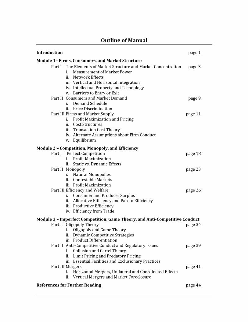
Outline of Manual

Introduction page 1

Module 1– Firms, Consumers, and Market Structure

Part I The Elements of Market Structure and Market Concentration page 3 i. Measurement of Market Power ii. Network Effects iii. Vertical and Horizontal Integration iv. Intellectual Property and Technology v. Barriers to Entry or Exit

Part II Consumers and Market Demand page 9 i. Demand Schedule ii. Price Discrimination

Part III Firms and Market Supply page 11 i. Profit Maximization and Pricing ii. Cost Structures iii. Transaction Cost Theory iv. Alternate Assumptions about Firm Conduct v. Equilibrium

Module 2 – Competition, Monopoly, and Efficiency Part I Perfect Competition page 18

i. Profit Maximization ii. Static vs. Dynamic Effects

Part II Monopoly page 23 i. Natural Monopolies ii. Contestable Markets iii. Profit Maximization

Part III Efficiency and Welfare page 26 i. Consumer and Producer Surplus ii. Allocative Efficiency and Pareto Efficiency iii. Productive Efficiency iv. Efficiency from Trade

Module 3 – Imperfect Competition, Game Theory, and Anti-Competitive Conduct Part I Oligopoly Theory page 34

i. Oligopoly and Game Theory ii. Dynamic Competitive Strategies iii. Product Differentiation

Part II Anti-Competitive Conduct and Regulatory Issues page 39 i. Collusion and Cartel Theory ii. Limit Pricing and Predatory Pricing iii. Essential Facilities and Exclusionary Practices

Part III Mergers page 41 i. Horizontal Mergers, Unilateral and Coordinated Effects ii. Vertical Mergers and Market Foreclosure

References for Further Reading page 44

Introduction:

The Role of Industrial Organization in Competition Law

1 | P a g e

The Origins of Industrial Organization

Microeconomics is the branch of Economics which studies how individual decision-

makers, such as firms or households, trade off costs and benefits to arrive at the

decisions they make. Microeconomics also studies the markets in which individuals

transact those decisions. Market observers since the days of Adam Smith have

known that the number of firms and firm profits vary widely across different

markets, and that in most markets there are some impediments to competition.

Industrial Organization is the field of Microeconomics which has been developed to

study the markets and firms in these imperfectly competitive environments.

The motivation for studying imperfect competition arose directly from the

competition law which developed in the United States and European Union in the

20th century. The U.S. Sherman Act of 1890 initiated modern competition law by

prohibiting contracts or other actions in restraint of trade. The prohibition of

restraint of trade dates back almost 500 years before the Sherman Act, to its

founding in English common law.

In addition to prohibiting restraint of trade, the Sherman Act made it a crime to

monopolize or attempt to monopolize a market. Legislators were motivated to limit

monopolies and promote competition because the higher prices associated with

monopoly inefficiently limit trade. In practice, attempts to monopolize or restrain

trade can be difficult to identify, and competition law has advanced greatly in

specifics since the Sherman Act. However, collusion to raise prices and cartel

behavior are prohibited under current competition law in the U.S. and E.U. alike.

Although competition laws around the world are not identical, they share the same

motivation for promoting competition and consumer welfare. For example, one way

in which European competition law has evolved differently from U.S. law is that E.U.

law also regulates the aid which member states give their national companies.

Early research in Industrial Organization focused on the “Structure-conduct-

performance” approach. Data from many industries showed a correlation between

market structure, prices, and firm profits: in markets with fewer firms, prices

tended to be higher and profits tended to be higher as well. In the mid-20th century,

regulators focused their concern on markets with few competitors. However,

economics research revealed how firms with large market shares could have higher

profits because of greater efficiency, lower costs, or better management. In many

situations where costs are cut, firms can make higher profits and consumers can

benefit from lower prices, so there is no need to assume that “correlation indicates

Introduction:

The Role of Industrial Organization in Competition Law

2 | P a g e

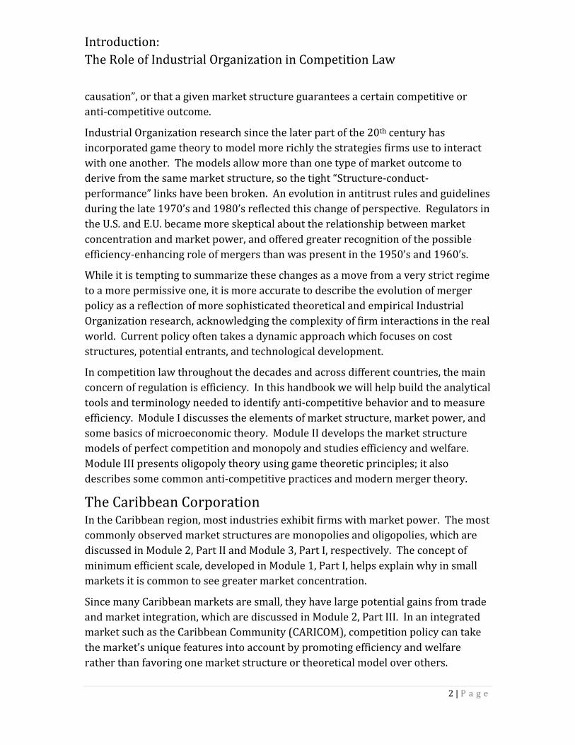
causation”, or that a given market structure guarantees a certain competitive or

anti-competitive outcome.

Industrial Organization research since the later part of the 20th century has

incorporated game theory to model more richly the strategies firms use to interact

with one another. The models allow more than one type of market outcome to

derive from the same market structure, so the tight “Structure-conduct-

performance” links have been broken. An evolution in antitrust rules and guidelines

during the late 1970’s and 1980’s reflected this change of perspective. Regulators in

the U.S. and E.U. became more skeptical about the relationship between market

concentration and market power, and offered greater recognition of the possible

efficiency-enhancing role of mergers than was present in the 1950’s and 1960’s.

While it is tempting to summarize these changes as a move from a very strict regime

to a more permissive one, it is more accurate to describe the evolution of merger

policy as a reflection of more sophisticated theoretical and empirical Industrial

Organization research, acknowledging the complexity of firm interactions in the real

world. Current policy often takes a dynamic approach which focuses on cost

structures, potential entrants, and technological development.

In competition law throughout the decades and across different countries, the main

concern of regulation is efficiency. In this handbook we will help build the analytical

tools and terminology needed to identify anti-competitive behavior and to measure

efficiency. Module I discusses the elements of market structure, market power, and

some basics of microeconomic theory. Module II develops the market structure

models of perfect competition and monopoly and studies efficiency and welfare.

Module III presents oligopoly theory using game theoretic principles; it also

describes some common anti-competitive practices and modern merger theory.

The Caribbean Corporation In the Caribbean region, most industries exhibit firms with market power. The most

commonly observed market structures are monopolies and oligopolies, which are

discussed in Module 2, Part II and Module 3, Part I, respectively. The concept of

minimum efficient scale, developed in Module 1, Part I, helps explain why in small

markets it is common to see greater market concentration.

Since many Caribbean markets are small, they have large potential gains from trade

and market integration, which are discussed in Module 2, Part III. In an integrated

market such as the Caribbean Community (CARICOM), competition policy can take

the market’s unique features into account by promoting efficiency and welfare

rather than favoring one market structure or theoretical model over others.

Module 1:

Firms, Consumers, and Market Structure

3 | P a g e

PART I

The Elements of Market Structure and Market Concentration

Although market structure itself is not the sole determinant of market outcomes,

understanding the market’s structure is crucial for modeling firm behavior. Some of the

main elements of market structures which are most important for analyzing competitive

effects are found in Table 1.

TABLE 1

Industrial Organization studies markets and firms in imperfect competition, which is

characterized by one or more of the firms exhibiting market power.

Definition: A firm has market power if it is able to sell its products at a price which exceeds

its marginal cost.

The Lerner index is a formal measure of market power, defined as:

��

We will discuss typical firm cost structure more below. The main idea behind the market

power definition is that in the most competitive markets, many firms will enter until price

is driven down to marginal cost. When price equals marginal cost, firms are making zero

economic profit so they are just indifferent between staying in the market and leaving the

market.1 Hence, saying that a firm has market power is equivalent to saying the market

does not exhibit “perfect competition,” which we will describe in Part I of Module 2 below.

1 When economists say that a firm has “zero profit,” what they usually mean is that the firm

has a “very small accounting profit but zero economic profit.” The difference between economic and accounting profit is that the former takes into account the opportunity cost of doing business while the later only considers balance-sheet costs. A firm’s opportunity cost is the benefit of their next-best option. This is a technical point since opportunity cost is almost always unobservable to a regulator or researcher. The main point to remember is, “zero profit” in perfect competition can also be thought of as “almost-zero profit.”

Definition ............................... What products and geographies are included?

Firms ................................................................................ Who sells the products?

Consumers ............................................................................... Who buys the products?

Product type ............................. Differentiated or homogeneous across sellers?

Elasticity of demand ............................... How sensitive is demand to changes in price?

Elements of Market Structure

Module 1:


4 | P a g e

If one or more firms in a market exhibit market power, this is evidence that the market is

concentrated. Two common ways of measuring market concentration are the Herfindahl-

Hirschman Index (also called HHI) and the C-4. The HHI for a market with F firms is

defined as:

��

��

In the equation above, Sf denotes the share of firm f. HHI ranges from 0 to 10,000, with

higher HHI’s associated with greater market concentration. In a monopoly market with

only one firm whose Sf =100, HHI is at its maximum: (100)2 = 10,000. The C-4 measure is

simply equal to the sum of the shares of the four firms with the largest shares.

Table 2 lists the market structure elements most often correlated with large market power.

The most important factor in determining market power is the last one on the list: price

elasticity of demand, which is often abbreviated to “elasticity of demand.”

Definition: The price elasticity of demand is the percentage change in demand that would

occur if the price changed by 1%.

Elasticity of demand measures demand’s sensitivity to changes in price. If demand is not

very sensitive to changes in price, the elasticity of demand is small and the firm has market

power. The Lerner index measure of market power can actually be expressed in terms of

the price elasticity alone, where Ed is the price elasticity of demand facing the firm:

��

TABLE 2

The key connection between price elasticity of demand and the other items in the list is the

number of substitute products available to consumers. When more substitutes are

available, the elasticity of demand is smaller and market power is lower. We can see how

each of the first four elements in Table 2 is associated with fewer possible substitutes.

Definition........... Narrower, with fewer products and smaller geographies

Firms ............................................................................................................ Fewer firms

Consumers .................................................................................................... Fewer (usually)

Product type ................................................................ Greater product differentiation

Elasticity of demand ........................................ Demand less sensitive to changes in price

Market Structure Elements Generally Associated with Greater Market Power

Module 1:


5 | P a g e

• If we define the market narrowly, we are explicitly making the number of potential

substitutes smaller. For example, if we are studying a merger between two

telecommunications companies who make smart phones, and we consider the market

to be very broad, including “all video communication services” (which would include

smart phones, internet phone services, and video teleconference services), we would

assert that the consumers in this market have more substitutes for smart phones than if

we define the market more narrowly as “portable video and e-mail devices” (which

would exclude from the market internet phone services or other services that relied on

Wi-Fi rather than satellite connectivity).

Market definition can determine whether or not a proposed merger is approved. For

example, the U.S. Federal Commerce Commission’s review of the proposed merger

between XM and Sirius in 2007 and 2008 hinged on market definition. If the market

had been viewed narrowly as “satellite radio” the two merging firms would have had a

combined market share of 100%. The firms argued that significant substitutability

existed between satellite radio and non-satellite streaming music services, and this

broader definition of the market was integral to the merger’s approval.

• If there are fewer firms in the market, there will almost always be fewer substitutes

available to consumers. In markets with differentiated products (which will be

discussed later in Module 3), a firm may find it optimal to offer different versions of the

same product. However, since to some extent a firm’s products always compete with

and potentially “cannibalize” sales of their other products in the market, fewer firms

will offer fewer total products.

• If there are fewer consumers in a market, there will most likely be fewer firms serving

that market and fewer substitutes available. The correlation between market size and

number of firms arises from the existence of a “minimum efficient scale” in long-run

profit maximization.

Definition: The minimum efficient scale for a firm is the smallest output level which

minimizes long-run average total cost.

Why does such a scale exist? Firms that are operating below minimum efficient scale

could decrease their average cost (and hence increase their profit) by increasing output.

No opportunity to increase profit is overlooked in the long run, so no firm will operate

at a scale smaller than minimum efficient scale in the long run. Cost-savings from

capital investments are one of the main reasons why average cost falls as total output

rises; we will discuss this aspect of firm cost structure more in Part III.

Table 3 illustrates how minimum efficient scale causes the number of firms in a market

to be highly correlated with the number of consumers in the market. In Table 3, we

Module 1:


6 | P a g e

assume that the number of consumers in each market varies but the minimum efficient

scale for each firm is 200 units. We assume that for some equilibrium price, each

consumer demands 10 units. Total market demand is the product of number of

consumers and demand per consumer. The number of firms in each market in long-run

equilibrium is equal to the total market demand divided by the minimum efficient scale.

In this example the number of firms and number of consumers are perfectly

correlated—that is, we could calculate the equilibrium number of firms directly by

dividing the number of consumers by 20. While such an exact relationship would be

rare in the real world, a tight relationship is observed in most industries.

TABLE 3

• Greater product differentiation is also associated with fewer substitutes available to the

customer. Firms seek to differentiate their products in order to decrease their demand

elasticity and gain market power, giving them the ability to charge a higher price. For

example, if farmers all grow the same type of wheat, the product is homogeneous and

wheat consumers are likely to view wheat from one farmer as a perfect substitute for

wheat from another farmer. If, however, a savvy farmer can differentiate his wheat—

perhaps by advertising special attributes of his farm or its reputation for particularly

excellent wheat, the wheat customers might come to see that farmer’s wheat as

different from the rest. If such a differentiation can be made, the farmer makes the

competitors’ wheat a weaker substitute for his product, making the demand he faces

less elastic, his market power greater, and the price he can charge greater as well.

In real-world markets, firms exhibit market power for many other reasons less directly

related to market structure, including network effects, vertical and horizontal integration,

intellectual property, and barriers to entry or exit. We will describe each source of market

power below. Keep in mind that a firm can increase its market power by decreasing its

cost while keeping price constant just as easily as by decreasing price while keeping cost

constant. While high profits are often observed in markets where one firm has a large

Market

Number

of consumers

Demand per

consumer (units)

Total market

demand (units)

Number of firms

in long-run

equilibrium*

Market 1 60 10 600 3

Market 2 100 10 1000 5

Market 3 240 10 2400 12

Market 4 500 10 5000 25

*Note: Assumes that minimum efficient scale for every firm is 200 units.

Module 1:


7 | P a g e

market share, the profits might arise from the firm’s low costs or high efficiency—it doesn’t

necessarily mean the firm is “taking advantage” of inelastic demand.

Market Power Source 1: Network Effects

Network effects arise when the benefits to an individual consumer from using a product

are higher if there are greater numbers of other consumers using that product. Many

technologies demonstrate network effects. As an example, imagine that Company A is

considering buying e-mail service in two different scenarios. In the first scenario, only one

other firm has e-mail service. In the second scenario, almost every other company already

has e-mail service. The benefit to Company A of purchasing e-mail service would be much

larger in the second scenario than the first scenario, and accordingly, Company A would be

willing to pay much more for e-mail service in the second scenario. Once a product has

acquired a large network of users, the demand it faces can become less and less elastic.

Market Power Source 2: Intellectual Property

Firms often derive market power from owning intellectual property such as patents,

trademarks, or other brand copyrights. Legal limitations such as these directly limit the

proximity of substitutes that competitor firms can offer. Brand trademarks also reinforce a

product’s differentiation and ensure that consumers can’t find an exact substitute.

Intellectual property is most likely to increase market power by decreasing the elasticity of

demand faced by the firm, which means that consumer demand is less responsive to price

changes. We will discuss a model of imperfect competition in Module 3 in which firms’

intellectual property research is a form of strategic competition.

Market Power Source 3: Vertical or horizontal integration

Vertical and horizontal integration are forms of cost savings which can lead to market

power. Firms can become vertically integrated by buying their suppliers, developing their

own supply chain, or distributing their own products. Through any method, vertical

integration decreases costs because extra “layers” of mark-up can be eliminated. Figure 1

illustrates: the left-hand side supply chain shows Firm B supplying Firm A with no vertical

integration; on the right-hand side the two stages of production have been combined into

Firm A. The output price is the same ($170) and the initial input price is the same ($10),

but Firm A earns a higher profit in the integrated right-hand side supply chain.

Module 1:


8 | P a g e

FIGURE 1: Illustration of Vertical Integration

Alternately, firms can become horizontally integrated by expanding their market share in a

given stage of production. Horizontal integration can also lead to costs savings, perhaps by

sharing overhead, taking advantage of a larger scale of operation, or expanding into new

geographic or specialty markets. We discuss mergers which increase horizontal

integration in Module 3, Part III.

Market Power Source 4: High Barriers to Entry or Exit

Market power often arises from barriers to exit or entry. Barriers to entry protect firms’

high profits by precluding new firms from becoming competitors. Such barriers may

include large capital requirements, high advertising expenditure by the incumbent firm(s),

or other restrictions such as licensing.

The large amount of capital required to enter some industries, such as airlines or

telecommunications, limits the number of potential entrant firms to those who have

enough capital. Since many costs may be “sunk,” and not retrievable upon exit from the

industry, this may be a further deterrent to entry. Exit costs may also include severance

Stage 1 of production

(Firm B)

Input costs: $10Value added:

$90Mark-up: $10

Output price: $110

Stage 2 of

production(Firm A)

Input costs: $110

Value added: $50

Mark-up: $10

Output price: $170

Single stage of production

(Firm A)

Input costs: $10

Value added:

$140Mark-up: $20Output price:

$170

No integration

Firm A mark-up: $10

IntegrationFirm A mark-up: $20

Module 1:


9 | P a g e

pay for employees. Exit costs and sunk costs can be barriers to entry because they increase

the cost associated with the risk of failure to be profitable.

An incumbent firm can also create barriers to entry by investing heavily in advertising. If

the firm can establish a loyal following for itself among consumers, it may leave potential

entrants with little demand “leftover” for them if they enter.

Licensing restrictions are commonly seen as a form of barrier to entry in the labor market.

Instead of firms selling products, this market features individuals selling their labor to

firms; however, many of the economic principles introduced in these Modules apply to the

labor market. For example, medical professionals, salon workers, teachers, and workers in

some trades must obtain licenses to perform their jobs. Licensure may require monetary

or time costs, and some individuals may not be able to pass every licensing test. All of these

factors decrease the pool of potential entrants to these fields, which helps the workers

currently in the fields attain higher salaries.

PART II

Consumers and Market Demand

Let’s take a step back and review the fundamental building blocks of a market system:

supply and demand. Often, we think of firms in the role of suppliers and households in the

role of “demanders” or consumers, but firms can also be consumers (think of the large

fraction of economic activity that reflects business-to-business transactions) and

households often sell products and services, including their labor.

Definition: Demand is the quantity that consumers want to buy at a given price.

For most goods and services in the world, quantity demanded increases as price decreases.

For example, as the price of personal music players has decreased over time, more and

more individuals have purchased them.2 If we can observe the level of demand for a

number of different prices, we can plot out a demand curve. For example, suppose we have

the following data from the market for personal music players:

2 Obviously, the average price of a player is not the only thing that has changed over time in the personal music industry. However, we must assume that “all else is equal” in order to claim that we are isolating the effect of price only on demand. In some situations this assumption is more realistic than others. Here we are assuming it holds for the sake of the example.

Module 1:


10 | P a g e

FIGURE 2: Demand for Personal Music Players

Figure 2 plots the schedule for market demand. As we saw in Table 3 above, market

demand is the sum of the individual demand of all consumers in the market. While for

some analyses it is convenient and appropriate to assume as we did in Table 3 that all

consumers have the exact same demand for a given price, it is more realistic to assume that

individual consumers have different demand curves.

Suppose the market consists of just two households, Household K and Household J, with

the following individual demand schedules:

Price

(€)

Demand

(Quantity, millions)

100 0.5

80 1.0

60 2.0

40 4.0

20 5.5

Price

Quantity

20

60

100

80

40

120

1 53 42

Demand

Household K Household J

Price

(€)

Demand

(Quantity, units)

Price

(€)

Demand

(Quantity, units)

100 0 100 1

80 1 80 2

60 2 60 3

30 3 30 4

20 4 20 5

Module 1:


11 | P a g e

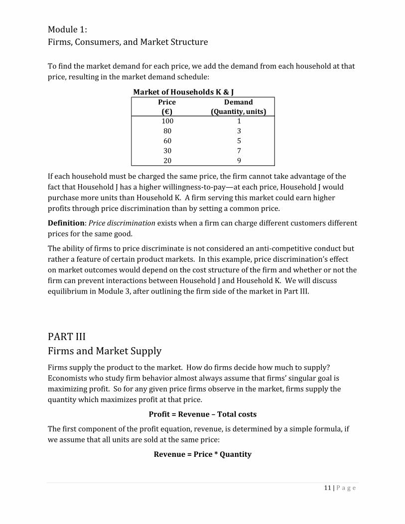
To find the market demand for each price, we add the demand from each household at that

price, resulting in the market demand schedule:

If each household must be charged the same price, the firm cannot take advantage of the

fact that Household J has a higher willingness-to-pay—at each price, Household J would

purchase more units than Household K. A firm serving this market could earn higher

profits through price discrimination than by setting a common price.

Definition: Price discrimination exists when a firm can charge different customers different

prices for the same good.

The ability of firms to price discriminate is not considered an anti-competitive conduct but

rather a feature of certain product markets. In this example, price discrimination’s effect

on market outcomes would depend on the cost structure of the firm and whether or not the

firm can prevent interactions between Household J and Household K. We will discuss

equilibrium in Module 3, after outlining the firm side of the market in Part III.

PART III

Firms and Market Supply

Firms supply the product to the market. How do firms decide how much to supply?

Economists who study firm behavior almost always assume that firms’ singular goal is

maximizing profit. So for any given price firms observe in the market, firms supply the

quantity which maximizes profit at that price.

Profit = Revenue – Total costs

The first component of the profit equation, revenue, is determined by a simple formula, if

we assume that all units are sold at the same price:

Revenue = Price * Quantity

Market of Households K & J

Price

(€)

Demand

(Quantity, units)

100 1

80 3

60 5

30 7

20 9

Module 1:


12 | P a g e

If a firm can price discriminate, the formula for revenue follows the same intuition but we

have to calculate the customer-level revenues first and then add them together to find total

revenue. For example, if the firm has four customers and customer 1 buys Quantity1 at

Price1, customer 2 buys Quantity2 at Price2, etcetera, the formula would be:

Revenue = Price1*Quantity1 + Price2*Quantity2+ Price3*Quantity3+ Price4*Quantity4

The second component of the profit equation, total cost, can be divided into two categories:

fixed costs and variable costs.

Total cost = Variable cost + Fixed cost

Variable costs are expenses which relate to the quantity of product the firm is producing.

Fixed costs are expenses which do not depend on the firm’s production level. For example,

for a firm that manufactures items such as apparel, variable costs might include cloth,

buttons, or labor used to produce each unit. Fixed costs for such a firm might be the rental

price they pay for their plant or the annual fee they pay to a trade association. In the real

world, many inputs are “lumpy” so their payment is a sort of blend between fixed and

variable cost. The manufacturing plant could be a lumpy input; for the large range of units

that can be produced in that plant, the plant cost is fixed, but increasing output past the

capacity of the plant requires incurring a large fixed expense.

Figure 3 shows how average costs per unit change as output quantity increases.

FIGURE 3: A Typical Firm Cost Structure

$/unit

Quantity Produced

Average Variable Cost

(AVC)

Average Fixed Cost

(AFC)

Average Total Cost

(ATC)

Marginal Cost

(MC)

Module 1:


13 | P a g e

In Figure 3, average fixed cost is decreasing over the entire range of output because the

same dollar amount of cost is being spread over more and more units. This intuition

explains why firms always try to “spread their overhead”—they are trying to decrease their

average fixed cost. Average variable cost is decreasing over a low range of output, because

the firm can take advantage of economies of scale in this range.

Definition: Economies of scale exist for a firm when the cost per unit decreases as the total

number of units produced increases.

Economies of scale often exist because as a firm expands its production it can invest in

capital which is more efficient. For example, economies of scale exist in the agriculture

industry because machines can harvest produce more efficiently than humans, but a firm

will only use mechanical harvesters if it is producing a large quantity.

Average total cost (ATC) is the sum of average variable cost (AVC) and average fixed cost

(AFC). Initially, ATC falls quickly since both AVC and AFC are decreasing. As output rises,

fixed costs contribute less and less to total cost, so the variable and total cost curves will be

closer and closer together.

In the long run, economies of scale are what determine the minimum efficient scale as

described in Part I above. If we imagine a curve passing through the lowest point of the

average total cost curves for many differently- sized scales of operation, this would trace

out the Long-Run Average Total Cost (LRATC) curve. Figure 4 illustrates the concept of the

LRATC curve. If all the firms in an industry had the LRATC shown in Figure 4, in the long

run they would all operate at the Q2 scale since it achieves the lowest ATC possible.

FIGURE 4: A Typical Long-Run Cost Structure

$/unit

Long-Run Average Total Cost(LRATC)

Short-Run

ATC(Scale Q1)

Short-Run

ATC(Scale Q2)

Short-Run

ATC(Scale Q3)

Quantity Produced

Q2 Q3Q1

Module 1:


14 | P a g e

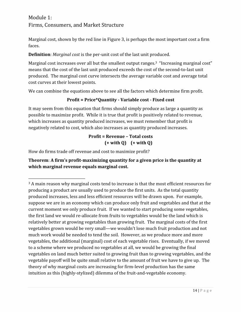
Marginal cost, shown by the red line in Figure 3, is perhaps the most important cost a firm

faces.

Definition: Marginal cost is the per-unit cost of the last unit produced.

Marginal cost increases over all but the smallest output ranges.3 “Increasing marginal cost”

means that the cost of the last unit produced exceeds the cost of the second-to-last unit

produced. The marginal cost curve intersects the average variable cost and average total

cost curves at their lowest points.

We can combine the equations above to see all the factors which determine firm profit.

Profit = Price*Quantity - Variable cost - Fixed cost

It may seem from this equation that firms should simply produce as large a quantity as

possible to maximize profit. While it is true that profit is positively related to revenue,

which increases as quantity produced increases, we must remember that profit is

negatively related to cost, which also increases as quantity produced increases.

Profit = Revenue – Total costs

(+ with Q) (+ with Q)

How do firms trade off revenue and cost to maximize profit?

Theorem: A firm’s profit-maximizing quantity for a given price is the quantity at

which marginal revenue equals marginal cost.

3 A main reason why marginal costs tend to increase is that the most efficient resources for

producing a product are usually used to produce the first units. As the total quantity

produced increases, less and less efficient resources will be drawn upon. For example,

suppose we are in an economy which can produce only fruit and vegetables and that at the

current moment we only produce fruit. If we wanted to start producing some vegetables,

the first land we would re-allocate from fruits to vegetables would be the land which is

relatively better at growing vegetables than growing fruit. The marginal costs of the first

vegetables grown would be very small—we wouldn’t lose much fruit production and not

much work would be needed to tend the soil. However, as we produce more and more

vegetables, the additional (marginal) cost of each vegetable rises. Eventually, if we moved

to a scheme where we produced no vegetables at all, we would be growing the final

vegetables on land much better suited to growing fruit than to growing vegetables, and the

vegetable payoff will be quite small relative to the amount of fruit we have to give up. The

theory of why marginal costs are increasing for firm-level production has the same

intuition as this (highly-stylized) dilemma of the fruit-and-vegetable economy.

Module 1:


15 | P a g e

When the firm is at a profit-maximizing price-quantity pair and marginal revenue equals

marginal cost, this means that the last unit offered for sale earns zero profit. Since

marginal cost increases as quantity increases, and marginal revenue stays the same or

decreases as quantity increases (as we will see in Module 2), the next unit would

hypothetically have marginal revenue less than marginal cost. This hypothetical next unit

is not offered for sale because it would have marginal revenue less than marginal cost and

hence would not increase profit.

Given the assumption of profit-maximization, the firm’s optimal equation of marginal

revenue and marginal cost is universally accepted by economists. However, economists

have also studied firm behavior under other assumptions about firm goals, and tried to

answer a bigger question—why do firms exist at all? That is, why isn’t all market supply

generated by entrepreneurs who maximize profit for their own benefit instead of the firm

and shareholders’ benefit? The economist Ronald Coase posited an important answer to

this question in 1937 with his development of Transaction Cost Theory. He argued that

entrepreneurs must face transaction costs in order to do business in a marketplace, and

these costs can be avoided by transacting some exchanges within a firm instead of on the

marketplace. Transaction costs include search costs necessary for learning about what

prices or goods are available, regulatory costs such as legal fees, or commission fees paid to

make an exchange on a market. In Coase’s model, firms’ existence and sizes arise from

their optimal balancing of internal and external transaction costs.

More recent developments in the field of Organizational Behavior, a field of

Microeconomics closely related to Industrial Organization but more concerned with the

inner workings of the firm, have expanded on Coase’s insights. Broader ideas of how firms

behave have been explored, and many possible goals besides pure profit maximization

have been identified. For example, in a firm with a manager who is not the owner, the

manager could be modeled as a maximizer of his own salary or enjoyment rather than firm

profit. This gives rise to the well-known “Principle-Agent Problem” in which the Principle

(the firm owners or shareholders) must give the Agent (the manager) incentives to act in

the best interest of the Principle even though the Principle cannot perfectly observe the

Agent’s behavior. Behavioral-based theories have also been developed which model the

manager as an imperfect profit-maximizer, limited by his own cognitive ability and unable

to take into account every single aspect of every decision.

Module 1:


16 | P a g e

We finish Module 1 by returning to the simple example from the market for music players.

We plotted the demand schedule in Figure 2 and now describe its counterpart, the supply

schedule.

Definition: Supply is the quantity that producers are willing to sell at a given price.

For most goods and services in the world, quantity supplied decreases as price decreases.

If we can find the level of supply for a number of different prices, we can plot out a supply

curve. Suppose we have the following market data:

FIGURE 5: Supply for Personal Music Players

Figure 5 plots the supply schedule.

In a market of buyers and sellers, equilibrium is reached when the quantity demanded by

the buyers equals the quantity supplied by the sellers. Combining Figure 2 and Figure 5,

we see that equilibrium is reached where the supply and demand curves intersect. In our

example, the equilibrium price is € 2 which corresponds to the equilibrium quantity, 2

million.

Price

(€)

Supply

(Quantity, millions)

100 5.0

80 3.5

60 2.0

40 1.0

20 0.5

Price

Quantity

20

60

100

80

40

120

1 53 42

`

Supply

Module 1:


17 | P a g e

FIGURE 6: Equilibrium in the Market for Personal Music Players

The stylized example we have just worked through serves only as intuition. In Module 2

we will explore what equilibrium looks like in two very different market structures, perfect

competition and monopoly. We will build on the main concepts in Module 1.

Price

Quantity

20

60

100

80

40

120

1 53 42

`

Supply

Demand

● Demand decreases as price increases, if all else is held constant.

● Firms' market supply is chosen as a result of profit maximization.

● Firms set market supply where marginal revenue equals marginal cost.

● Equilibrium exists in a market when quantity demanded equals quantity supplied.

Module 1 Take-Aways

Module 2:

Competition, Monopoly, and Efficiency

18 | P a g e

PART I

Perfect Competition

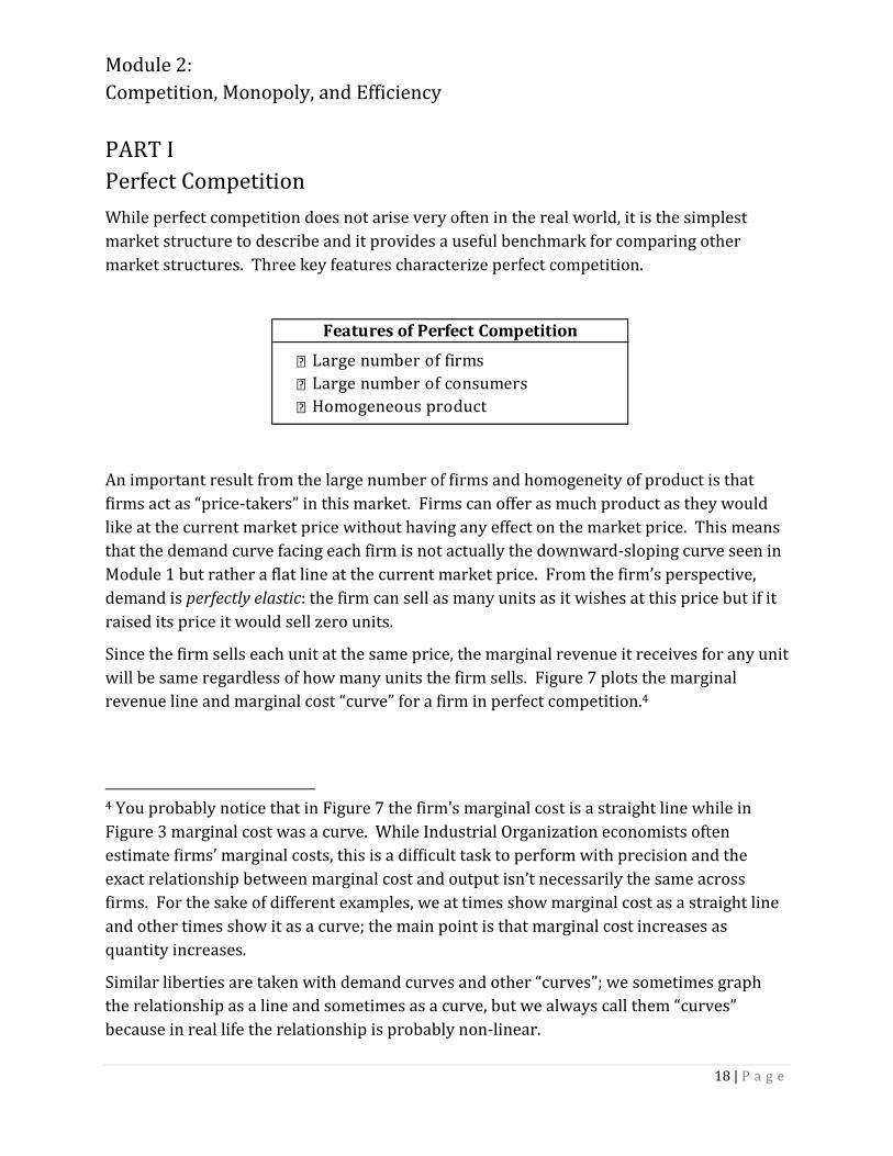
While perfect competition does not arise very often in the real world, it is the simplest

market structure to describe and it provides a useful benchmark for comparing other

market structures. Three key features characterize perfect competition.

An important result from the large number of firms and homogeneity of product is that

firms act as “price-takers” in this market. Firms can offer as much product as they would

like at the current market price without having any effect on the market price. This means

that the demand curve facing each firm is not actually the downward-sloping curve seen in

Module 1 but rather a flat line at the current market price. From the firm’s perspective,

demand is perfectly elastic: the firm can sell as many units as it wishes at this price but if it

raised its price it would sell zero units.

Since the firm sells each unit at the same price, the marginal revenue it receives for any unit

will be same regardless of how many units the firm sells. Figure 7 plots the marginal

revenue line and marginal cost “curve” for a firm in perfect competition.4

4 You probably notice that in Figure 7 the firm’s marginal cost is a straight line while in

Figure 3 marginal cost was a curve. While Industrial Organization economists often

estimate firms’ marginal costs, this is a difficult task to perform with precision and the

exact relationship between marginal cost and output isn’t necessarily the same across

firms. For the sake of different examples, we at times show marginal cost as a straight line

and other times show it as a curve; the main point is that marginal cost increases as

quantity increases.

Similar liberties are taken with demand curves and other “curves”; we sometimes graph

the relationship as a line and sometimes as a curve, but we always call them “curves”

because in real life the relationship is probably non-linear.

● Large number of firms

● Large number of consumers

● Homogeneous product

Features of Perfect Competition

Module 2:


19 | P a g e

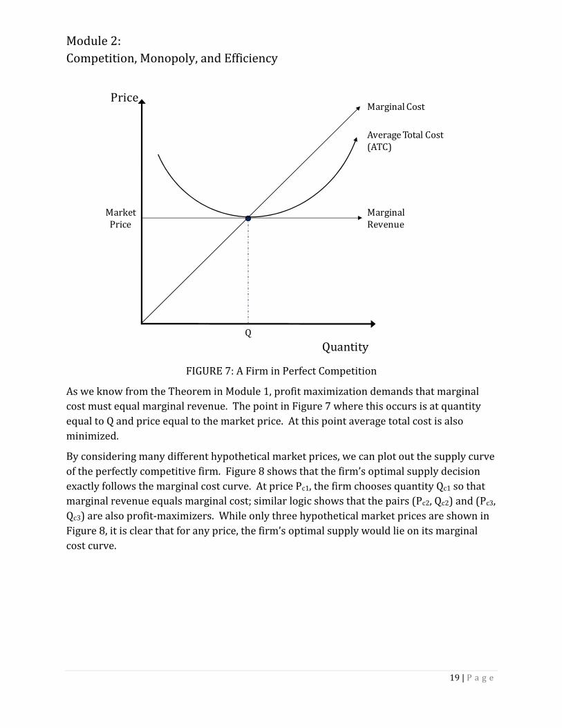
FIGURE 7: A Firm in Perfect Competition

As we know from the Theorem in Module 1, profit maximization demands that marginal

cost must equal marginal revenue. The point in Figure 7 where this occurs is at quantity

equal to Q and price equal to the market price. At this point average total cost is also

minimized.

By considering many different hypothetical market prices, we can plot out the supply curve

of the perfectly competitive firm. Figure 8 shows that the firm’s optimal supply decision

exactly follows the marginal cost curve. At price Pc1, the firm chooses quantity Qc1 so that

marginal revenue equals marginal cost; similar logic shows that the pairs (Pc2, Qc2) and (Pc3,

Qc3) are also profit-maximizers. While only three hypothetical market prices are shown in

Figure 8, it is clear that for any price, the firm’s optimal supply would lie on its marginal

cost curve.

Price

Quantity

Marginal

Revenue

Marginal Cost

Market

Price

Q

Average Total Cost

(ATC)

Module 2:


20 | P a g e

FIGURE 8: The Supply Curve in Perfect Competition

If we also assume that all firms have the same technology, and hence have the same

marginal costs, the market supply in perfect competition is simply the number of firms

times the marginal cost of each firm. If we plot the market supply curve, it is simply a

scaled-up version of the firm supply curve. If we also assume a standard downward-

sloping demand curve for the market, we can find the equilibrium which is illustrated in

Figure 9. Equilibrium is at (P*, Q*) where supply equals demand.

Price

Quantity

Marginal

Revenue 1

Marginal Cost

= Supply

Pc1

Qc1

Marginal

Revenue 2Pc2

Marginal

Revenue 3Pc3

Qc2 Qc3

Module 2:


21 | P a g e

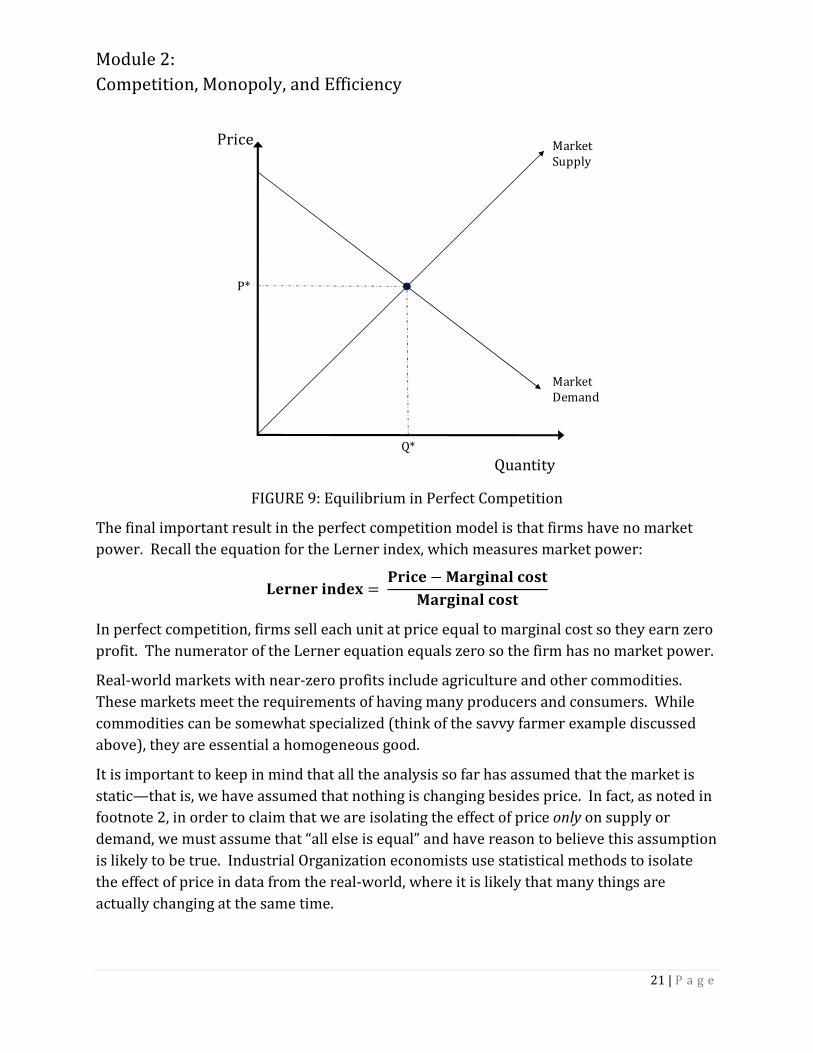
FIGURE 9: Equilibrium in Perfect Competition

The final important result in the perfect competition model is that firms have no market

power. Recall the equation for the Lerner index, which measures market power:

��

In perfect competition, firms sell each unit at price equal to marginal cost so they earn zero

profit. The numerator of the Lerner equation equals zero so the firm has no market power.

Real-world markets with near-zero profits include agriculture and other commodities.

These markets meet the requirements of having many producers and consumers. While

commodities can be somewhat specialized (think of the savvy farmer example discussed

above), they are essential a homogeneous good.

It is important to keep in mind that all the analysis so far has assumed that the market is

static—that is, we have assumed that nothing is changing besides price. In fact, as noted in

footnote 2, in order to claim that we are isolating the effect of price only on supply or

demand, we must assume that “all else is equal” and have reason to believe this assumption

is likely to be true. Industrial Organization economists use statistical methods to isolate

the effect of price in data from the real-world, where it is likely that many things are

actually changing at the same time.

Price

Quantity

Market

Supply

Q*

Market

Demand

P*

Module 2:


22 | P a g e

Some of the factors which increase demand in a dynamic way—that is, they increase the

demand level at every possible price—are changing consumer tastes, anticipated future

increases in price (so people “stock up” now), or growth in income. These factors can also

work in the opposite direction to decrease demand at every price. The relationship

between demand and consumer income is defined by an important measure, the income

elasticity of demand.

Definition: The income elasticity of demand for a good or service is the percentage change

in demand that would occur if consumer income increased by 1%.

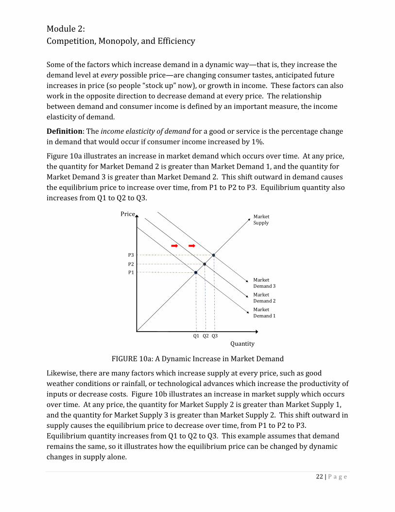
Figure 10a illustrates an increase in market demand which occurs over time. At any price,

the quantity for Market Demand 2 is greater than Market Demand 1, and the quantity for

Market Demand 3 is greater than Market Demand 2. This shift outward in demand causes

the equilibrium price to increase over time, from P1 to P2 to P3. Equilibrium quantity also

increases from Q1 to Q2 to Q3.

FIGURE 10a: A Dynamic Increase in Market Demand

Likewise, there are many factors which increase supply at every price, such as good

weather conditions or rainfall, or technological advances which increase the productivity of

inputs or decrease costs. Figure 10b illustrates an increase in market supply which occurs

over time. At any price, the quantity for Market Supply 2 is greater than Market Supply 1,

and the quantity for Market Supply 3 is greater than Market Supply 2. This shift outward in

supply causes the equilibrium price to decrease over time, from P1 to P2 to P3.

Equilibrium quantity increases from Q1 to Q2 to Q3. This example assumes that demand

remains the same, so it illustrates how the equilibrium price can be changed by dynamic

changes in supply alone.

Price

Quantity

Market

Supply

Q1

Market

Demand 1

P1

P2

P3

Q2 Q3

Market

Demand 2

Market

Demand 3

Module 2:


23 | P a g e

FIGURE 10b: A Dynamic Increase in Market Supply

PART II

Monopoly

In some respects, monopoly lies at the opposite end of the market structure spectrum from

perfect competition. In a monopoly market structure, only one firm sells the product to the

entire market. Pure monopolies can be found in real-world markets.

Legal factors can play an important role in forming monopolies. For example, if a national

market for a service is deemed crucial to national interests, a government may grant one

firm exclusive rights to the market. This situation has been observed in industries such as

air travel, telecommunications, national defense, and energy. Patents are a second source

of monopoly creation, although defending the claim that a firm is a monopolist relies

heavily on market definition. For example, if we define a market of “anti-depressants,” the

market would include many different firms selling many different prescription drugs.

However, if the market is defined as “drugs containing the chemical compounds found in

the anti-depressant Cymbalta,” the market is a monopoly, since the firm Eli Lilly holds a

patent on the prescription drug Cymbalta until 2013.

Two additional reasons why monopolies arise in real-world markets are economies of scale

and economies of scope. As described in Module 1, Part III, economies of scale exist if the

cost per unit decreases as the total number of units produced increases. If the minimum

Price

Quantity

Market

Supply 1

Q1

Market

Demand

P1

Market

Supply 2

Market

Supply 3

P2

P3

Q2 Q3

Module 2:


24 | P a g e

efficient scale for production is equal to the total size of the market, it is most efficient for a

single firm to service the whole market. This is the classic example of a “natural”

monopoly.

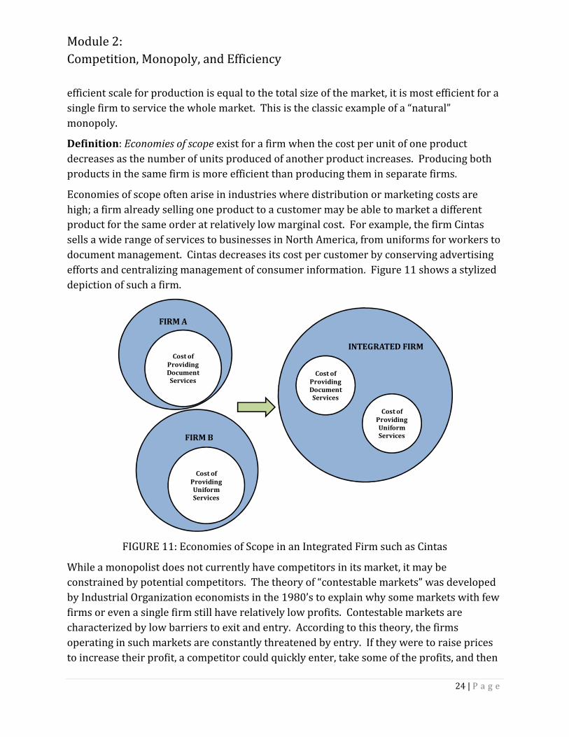
Definition: Economies of scope exist for a firm when the cost per unit of one product

decreases as the number of units produced of another product increases. Producing both

products in the same firm is more efficient than producing them in separate firms.

Economies of scope often arise in industries where distribution or marketing costs are

high; a firm already selling one product to a customer may be able to market a different

product for the same order at relatively low marginal cost. For example, the firm Cintas

sells a wide range of services to businesses in North America, from uniforms for workers to

document management. Cintas decreases its cost per customer by conserving advertising

efforts and centralizing management of consumer information. Figure 11 shows a stylized

depiction of such a firm.

FIGURE 11: Economies of Scope in an Integrated Firm such as Cintas

While a monopolist does not currently have competitors in its market, it may be

constrained by potential competitors. The theory of “contestable markets” was developed

by Industrial Organization economists in the 1980’s to explain why some markets with few

firms or even a single firm still have relatively low profits. Contestable markets are

characterized by low barriers to exit and entry. According to this theory, the firms

operating in such markets are constantly threatened by entry. If they were to raise prices

to increase their profit, a competitor could quickly enter, take some of the profits, and then

INTEGRATED FIRM

Cost of Providing Document Services

Cost of Providing Uniform Services

Cost of

Providing Document Services

Cost of

Providing Uniform Services

FIRM A

FIRM B

Module 2:


25 | P a g e

exit the market. Since the potential for increasing profit by raising prices is eliminated,

prices remain low in contestable markets even if they exhibit a monopoly market structure.

It is important to also realize that the monopolist is always constrained by market demand.

The statement that “they can charge as much as they want,” is a common but incorrect

description of monopolists’ behavior. The key feature of market demand which determines

how much profit a monopolist can optimally earn is the demand elasticity. Like all firms,

monopolists set marginal revenue equal to marginal cost in order to maximize profit.

The demand which the monopolist faces is the entire downward-sloping market demand

curve. While firms in perfect competition face inelastic demand at a price they take as

given, the monopolist can set its own price. Since market demand is elastic, the monopolist

can decrease its price to sell more units or increase its price to sell fewer units. This is

different from a firm’s situation in perfect competition, where it would sell zero units if it

raised its price above the market price.

The monopolist faces a trade-off: lowering its price will attract more consumers, but it will

also result in lower profit per consumer. If the firm cannot price discriminate and charge

consumers different prices, increasing its quantity sold requires decreasing the price on all

units sold. This causes the marginal revenue curve to lie below the demand curve, as

shown in Figure 12. The firm will set the equilibrium quantity Qm where the marginal cost

curve intersects the marginal revenue curve. Tracing the equilibrium quantity up to the

demand curve brings us to the equilibrium price, Pm.

FIGURE 12: Profit Maximization for a Monopolist

Price

Quantity

Demand

Marginal Cost

Qm

Pm

Marginal

Revenue

Module 2:


26 | P a g e

If we combine the equilibrium outcome in Figure 12 for monopoly with the outcome in

Figure 9 for perfect competition, we observe key differences: the equilibrium price is lower

in competition than in monopoly (Pc < Pm), and the equilibrium quantity is higher in

competition than in monopoly (Qc > Qm).

FIGURE 13: Monopoly and Perfect Competition Compared

We will explain in Part III why the difference in outcomes has implications for competition

policy.

PART III

Efficiency and Welfare

The definition and measurement of efficiency and welfare can take various forms, but they

constitute two goals of any competition policy.

Consumer surplus and producer surplus are two metrics which can be used to study

market efficiency.

Definition: Consumer surplus is the difference, measured in dollars, between the maximum

amount a consumer would have been willing to pay for a good or service and the actual

price they paid for it.

Price

Quantity

Pm

Pc

QcQm

Competitive

Supply =Marginal Cost

Demand

Marginal

Revenue

Module 2:


27 | P a g e

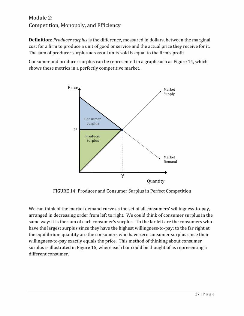
Definition: Producer surplus is the difference, measured in dollars, between the marginal

cost for a firm to produce a unit of good or service and the actual price they receive for it.

The sum of producer surplus across all units sold is equal to the firm’s profit.

Consumer and producer surplus can be represented in a graph such as Figure 14, which

shows these metrics in a perfectly competitive market.

FIGURE 14: Producer and Consumer Surplus in Perfect Competition

We can think of the market demand curve as the set of all consumers’ willingness-to-pay,

arranged in decreasing order from left to right. We could think of consumer surplus in the

same way: it is the sum of each consumer’s surplus. To the far left are the consumers who

have the largest surplus since they have the highest willingness-to-pay; to the far right at

the equilibrium quantity are the consumers who have zero consumer surplus since their

willingness-to-pay exactly equals the price. This method of thinking about consumer

surplus is illustrated in Figure 15, where each bar could be thought of as representing a

different consumer.

Price

Quantity

Market

Supply

Q*

Market

Demand

P*

Consumer Surplus

ProducerSurplus

Module 2:


28 | P a g e

FIGURE 15: Consumer Surplus Break-down

We could break down producer surplus in a similar way, with each bar representing a unit

of output. The first units of quantity produced have the lowest marginal cost so they

produce the greatest per-unit profit. The last unit to be produced, at the equilibrium

quantity, produces zero per-unit profit and adds nothing to producer surplus.

Consumer and producer surplus are defined the same way in all market structures, but

their graphical representations take different shapes. Figure 16 illustrates producer and

consumer surplus in a monopoly. Part of the area that was consumer surplus in perfect

competition has become producer surplus in monopoly, and both consumer and producer

surplus appear “truncated” at Qm because the units between Qm and Qc are no longer sold.

FIGURE 16: Producer and Consumer Surplus in Monopoly

Price

Market

DemandP*

Price

Quantity

Marginal

Revenue

Pm

Pc

QcQm

Competitive


Demand

ProducerSurplus

Consumer Surplus

Module 2:


29 | P a g e

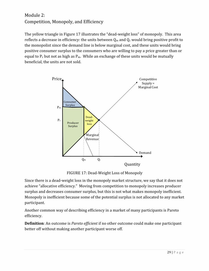
The yellow triangle in Figure 17 illustrates the “dead-weight loss” of monopoly. This area

reflects a decrease in efficiency: the units between Qm and Qc would bring positive profit to

the monopolist since the demand line is below marginal cost, and these units would bring

positive consumer surplus to the consumers who are willing to pay a price greater than or

equal to Pc but not as high as Pm. While an exchange of these units would be mutually

beneficial, the units are not sold.

FIGURE 17: Dead-Weight Loss of Monopoly

Since there is a dead-weight loss in the monopoly market structure, we say that it does not

achieve “allocative efficiency.” Moving from competition to monopoly increases producer

surplus and decreases consumer surplus, but this is not what makes monopoly inefficient.

Monopoly is inefficient because some of the potential surplus is not allocated to any market

participant.

Another common way of describing efficiency in a market of many participants is Pareto

efficiency.

Definition: An outcome is Pareto efficient if no other outcome could make one participant

better off without making another participant worse off.

Price

Quantity

Marginal

Revenue

Pm

Pc

QcQm

Competitive


Demand

ProducerSurplus

Consumer Surplus

Dead-weight

loss

Module 2:


30 | P a g e

Neither the allocative efficiency issue in monopoly nor the concept of Pareto efficiency has

anything to say about which participant’s surplus matters most or who should be made

better off. This is a question for policy-makers.

We discussed a third efficiency concept, productive efficiency, in Module 2, Part III without

stating its name. Productive efficiency requires that a firm chooses the output quantity

which minimizes average total costs, as shown in Figure 7. For an entire economy,

productive efficiency requires that every input is used as efficiently as possible. For

example, if we had data for the fruit and vegetable economy of footnote 3, we could find

one way to divide the land between growing fruit and growing vegetables which would

satisfy productive efficiency. No other way of dividing the land could produce greater total

output, measured in dollar terms.

International trade can be another source of efficiency gains. Gains from trade arise from

the principle of comparative advantage.

Definition: A producer (such as a firm, country, or individual) has a comparative advantage

in producing a good or service if the producer can make that item at a relatively lower cost,

compared to the producer’s next-best option.

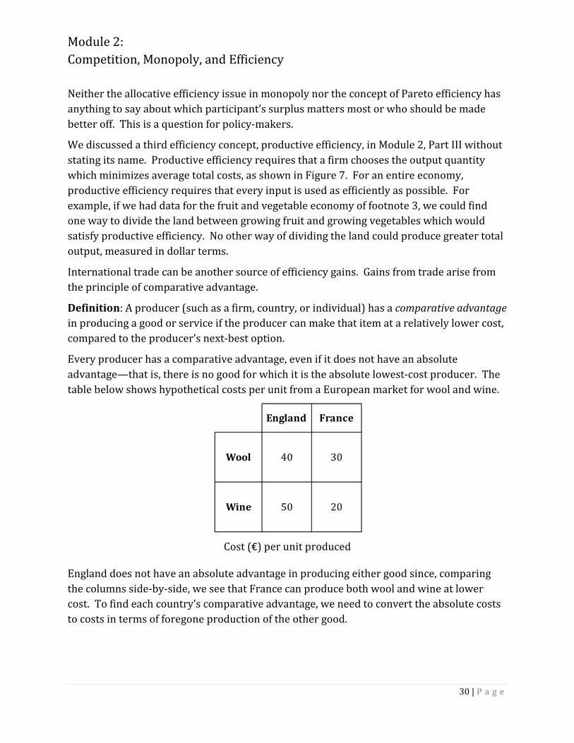
Every producer has a comparative advantage, even if it does not have an absolute

advantage—that is, there is no good for which it is the absolute lowest-cost producer. The

table below shows hypothetical costs per unit from a European market for wool and wine.

Cost (€) per unit produced

England does not have an absolute advantage in producing either good since, comparing

the columns side-by-side, we see that France can produce both wool and wine at lower

cost. To find each country’s comparative advantage, we need to convert the absolute costs

to costs in terms of foregone production of the other good.

England France

Wool 40 30

Wine 50 20

Module 2:


31 | P a g e

Cost per unit produced in terms of foregone other good:

The first value in the table shows the relative cost of wool in England: the value of the

inputs used to produce a unit of wool could have alternately been used to produce 40/50 =

0.80 units of wine. In France, the value of the inputs used to produce a unit of wool could

have produced 30/20 = 1.5 units of wine. By finding the smallest relative cost in each

country column, we find each country’s comparative advantage: England has a comparative

advantage in producing wool; France has a comparative advantage in producing wine.

Since trade brings efficiency gains through countries’ specialization in their comparative

advantage goods, promoting trade may be a policy goal. One way to promote trade is to

remove trade barriers by integrating markets. The table below outlines some of the

efficiency gains which can result from market integration.

Market integration may also increase welfare by decreasing transaction costs, as described

in Module 1, Part III. If the costs associated with market transactions decrease, a greater

number of mutually-beneficial transactions can be made.

England France

Wool

(in terms

of wine)

0.80 1.50

Wine

(in terms

of wool)

1.25 0.67

Result of market integration Efficiency gain

Factors of production such as land, labor,

and capital are allocated more efficiently Improves productive efficiency

Trade increasesImproves gains from comparative

advantage

Firms take advantage of economies of scale

because the market size has increasedImproves productive efficiency

Module 2:


32 | P a g e

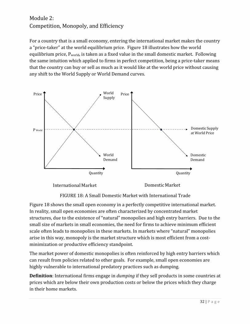
For a country that is a small economy, entering the international market makes the country

a “price-taker” at the world equilibrium price. Figure 18 illustrates how the world

equilibrium price, Pworld, is taken as a fixed value in the small domestic market. Following

the same intuition which applied to firms in perfect competition, being a price-taker means

that the country can buy or sell as much as it would like at the world price without causing

any shift to the World Supply or World Demand curves.

FIGURE 18: A Small Domestic Market with International Trade

Figure 18 shows the small open economy in a perfectly competitive international market.

In reality, small open economies are often characterized by concentrated market

structures, due to the existence of “natural” monopolies and high entry barriers. Due to the

small size of markets in small economies, the need for firms to achieve minimum efficient

scale often leads to monopolies in these markets. In markets where “natural” monopolies

arise in this way, monopoly is the market structure which is most efficient from a cost-

minimization or productive efficiency standpoint.

The market power of domestic monopolies is often reinforced by high entry barriers which

can result from policies related to other goals. For example, small open economies are

highly vulnerable to international predatory practices such as dumping.

Definition: International firms engage in dumping if they sell products in some countries at

prices which are below their own production costs or below the prices which they charge

in their home markets.

Price

Quantity

WorldSupply

World

Demand

P World

International Market

Price

Quantity

Domestic

Demand

Domestic Supplyat World Price

Domestic Market

Module 2:


33 | P a g e

Regulators of the small domestic economy may deter international firms from entering the

market in order to prevent the potential for dumping, since dumping would harm domestic

firms. Regulators of this economy may also wish to protect domestic monopolies for

political reasons.

Competition policy in a small open economy must weigh the potential production efficiency

gains from monopoly against the likelihood of higher prices and certain allocative

inefficiency (through deadweight loss) in monopoly.

While some markets in the real world do resemble perfect competition or monopoly, the

majority of markets are structured somewhere between these extremes. Between these

extremes lie oligopolistic market structures; Module III develops the theory of oligopoly.

Module 2 Take-Aways

● In perfect competition, firms are price-takers and the equilibrium price

equals the firms' marginal cost.

● Monopolies can arise in real-world markets through natural or legal means.

● Monopoly outcomes do not satisfy allocative efficiency because they result in

a deadweight loss.

● Trade and market integration can improve welfare through comparative

advantage and other efficiency gains.

Module 3:

Imperfect Competition, Game Theory, and Anti-Competitive Conduct

34 | P a g e

PART I

Oligopoly and Game Theory

The following table summarizes the key features of an oligopolistic market structure.

Oligopoly is the primary focus of Industrial Organization, and in real-world markets,

oligopoly is very common. For example, the markets for orange juice, toothpaste, blue

jeans, and computer chips could all be characterized as oligopolies.

Oligopoly models of competition usually assume that firms are competing in either price or

quantity, and they often use game theory. The key insight of game theory is that it models

each player’s payoff as a function of other players’ decisions. In a game theory model of

competition, the “players” are the firms and the “payoffs” are the firms’ profits. The firms’

“strategies” are the prices or quantities they intend to offer to the market.

In a price competition model, firm profits might be described by a table such as this:

Firm Y’s profits are the first in each pair: the profit to Firm Y if both firms choose Low price

is 5; the profit to Firm Y if Firm Y chooses a Low price but Firm Z chooses High price is 10.

Similarly, the profit to Firm Z if both firms choose High price is 7; the profit to Firm Z if

Firm Z chooses Low price but Firm Y chooses High price is 10. There is no need for the

profits to be symmetrical, but they happen to be in this example.

What will be the outcome of this game? The primary type of equilibrium in game theoretic

models is the Nash Equilibrium.

● Small number of firms

● Differentiated but substitutable products

● Firms face downward-sloping demand curve

● Firms compete using strategies

Features of Oligopoly

Low price High price

Low

price(5,5) (10,0)

High

price(0,10) (7,7)

Firm

Y

Firm Z

Module 3:


35 | P a g e

Definition: Firms’ strategies form a Nash Equilibrium if no firm could increase its profit by

choosing a different strategy, if it assumes the other firms keep the same strategies.

Is {Firm Y chooses Low price, Firm Z chooses High price} a Nash Equilibrium? It is not,

because if Firm Y assumed that Firm Z kept the strategy of High price, it could increase its

profit by choosing the High price strategy as well. The strategy pair {Firm Y chooses High

price, Firm Z chooses Low price} is not a Nash Equilibrium either by the same logic.

Is {Firm Y chooses High price, Firm Z chooses High price} a Nash Equilibrium? It is not,

because if Firm Y assumed that Firm Z kept the strategy of a High price, it could increase its

profit by choosing the Low price strategy.

The Nash Equilibrium to the game is that both firms will choose the Low price. If Firm Y

knows that Firm Z will choose the Low price, it could not make itself any better off by

switching to the High price. The same logic holds for Firm Z. Neither firm can “profitably

deviate” from their Low price choice, so this strategy pair is a Nash Equilibrium.

Price competition is often called “Bertrand competition,” named for the mathematician

who first modeled it.

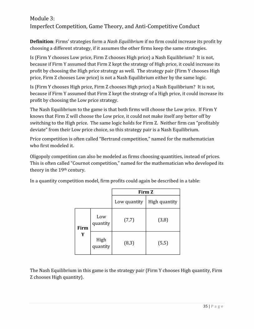
Oligopoly competition can also be modeled as firms choosing quantities, instead of prices.

This is often called “Cournot competition,” named for the mathematician who developed its

theory in the 19th century.

In a quantity competition model, firm profits could again be described in a table:

The Nash Equilibrium in this game is the strategy pair {Firm Y chooses High quantity, Firm

Z chooses High quantity}.

Low quantity High quantity

Low

quantity(7,7) (3,8)

High

quantity(8,3) (5,5)

Firm Z

Firm

Y

Module 3:


36 | P a g e

In the table, we see that profits are lower when output is higher. This is driven by the same

intuition of the supply shifts of Figure 10b—when supply increases but demand remains

the same, the equilibrium price must decrease.

The profit outcomes in the tables above portray a static view of the world. In reality, firms

do more than choose prices and quantities; at any given moment they are also undertaking

strategic actions which will affect their profit outcomes in the future.

Two strategies which firms use to increase their profits over time are (1) investing in

innovation and technology, and (2) investing in product differentiation.

Innovation and new technology can increase firms’ future profits in many ways: decreasing

costs and increasing efficiency, creating products to serve new niches, or improving a

current product so that consumers increase their willingness-to-pay. These benefits may

increase producer surplus, consumer surplus, or both. However, since these strategies

require current spending for future profit, firms with low or zero profits in the present may

not be able to undertake them. Additionally, firms might not be able to recoup their

investment expenses in a highly competitive market.

This argument provides intuition for why competition policies may allow monopolies in

innovation-dependent markets such as prescription drugs. As mentioned in Module 2, Part

II, the drug-maker Eli Lilly has a patent on the drug Cymbalta. It will continue earning a

monopoly profit until the patent expires. However, the development of the drug was a

large investment and some of the monopoly profit will go to cover that expense. Some of

the profit will also go into research for new drugs. The increase in consumer welfare

caused by the creation of new products can outweigh the efficiency or surplus losses from

higher prices due to market power.

In addition to patent creation, innovation can increase firm profit by finding technological

improvements which lead to cost savings. A key result of the Cournot model of quantity

competition is that if one of the firms decreases its costs, that firm will produce a greater

fraction of total output and increase its profit.

Product differentiation is also an important competitive strategy. As described in Module

1, Part I, product differentiation allows firms to increase their market power by making the

demand they face less elastic, and closer to a vertical line. Figure 19 shows how a change in

market demand from Demand 1 to Demand 2 causes the profit-maximizing price for the

same marginal cost curve to increase from P1 to P2.

Module 3:


37 | P a g e

FIGURE 19: Increase in Price with Decrease in Demand Elasticity

The decision of firms to differentiate their products can be modeled as a dynamic game.

FIGURE 20: A Dynamic Product Differentiation Game

Price

Quantity

Demand 1

Marginal Cost

P1

Marginal

Revenue 1

Demand 2

P2

Marginal

Revenue 2

Stage 1

Firms set their locations in product

space.

Stage 2

Firms engage in price competition

Two features of the price competition:

1. Competition is more aggressive and profits

are lower if the firms are located close together.

2. Demand is lower and profits are lower if

firms are located farther away from the most

popular locations in product space.

Module 3:


38 | P a g e

In Stage 2 of the game depicted in Figure 20, the first feature of price competition “pushes”

the firms to want to be farther apart in product space by being more differentiated. On the

other hand, the second feature of price competition “pulls” the firms towards the same

region of product space, since they want to choose product attributes that appeal to the

largest segment of the population.

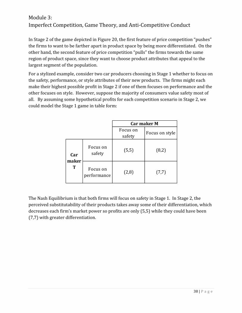
For a stylized example, consider two car producers choosing in Stage 1 whether to focus on

the safety, performance, or style attributes of their new products. The firms might each

make their highest possible profit in Stage 2 if one of them focuses on performance and the

other focuses on style. However, suppose the majority of consumers value safety most of

all. By assuming some hypothetical profits for each competition scenario in Stage 2, we

could model the Stage 1 game in table form:

The Nash Equilibrium is that both firms will focus on safety in Stage 1. In Stage 2, the

perceived substitutability of their products takes away some of their differentiation, which

decreases each firm’s market power so profits are only (5,5) while they could have been

(7,7) with greater differentiation.

Focus on

safetyFocus on style

Focus on

safety(5,5) (8,2)

Focus on

performance(2,8) (7,7)

Car maker M

Car

maker

T

Module 3:


39 | P a g e

PART II

Anti-Competitive Conduct and Regulatory Issues

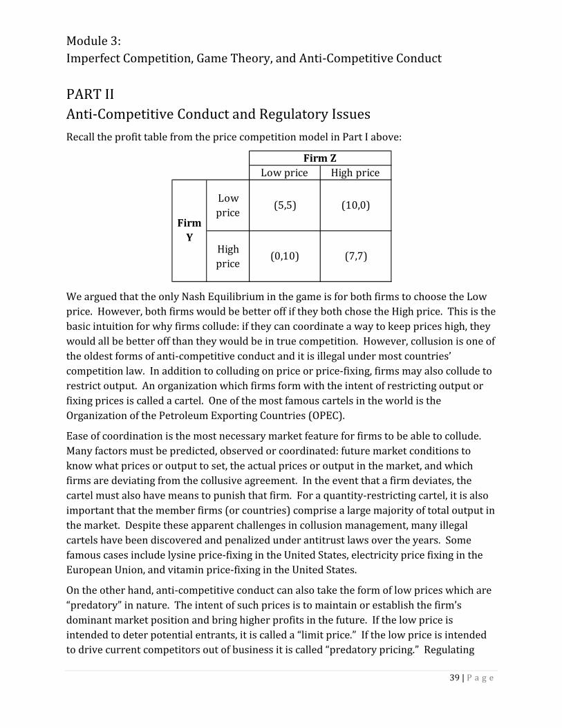
Recall the profit table from the price competition model in Part I above:

We argued that the only Nash Equilibrium in the game is for both firms to choose the Low

price. However, both firms would be better off if they both chose the High price. This is the

basic intuition for why firms collude: if they can coordinate a way to keep prices high, they

would all be better off than they would be in true competition. However, collusion is one of

the oldest forms of anti-competitive conduct and it is illegal under most countries’

competition law. In addition to colluding on price or price-fixing, firms may also collude to

restrict output. An organization which firms form with the intent of restricting output or

fixing prices is called a cartel. One of the most famous cartels in the world is the

Organization of the Petroleum Exporting Countries (OPEC).

Ease of coordination is the most necessary market feature for firms to be able to collude.

Many factors must be predicted, observed or coordinated: future market conditions to

know what prices or output to set, the actual prices or output in the market, and which

firms are deviating from the collusive agreement. In the event that a firm deviates, the

cartel must also have means to punish that firm. For a quantity-restricting cartel, it is also

important that the member firms (or countries) comprise a large majority of total output in

the market. Despite these apparent challenges in collusion management, many illegal

cartels have been discovered and penalized under antitrust laws over the years. Some

famous cases include lysine price-fixing in the United States, electricity price fixing in the

European Union, and vitamin price-fixing in the United States.

On the other hand, anti-competitive conduct can also take the form of low prices which are

“predatory” in nature. The intent of such prices is to maintain or establish the firm’s

dominant market position and bring higher profits in the future. If the low price is

intended to deter potential entrants, it is called a “limit price.” If the low price is intended

to drive current competitors out of business it is called “predatory pricing.” Regulating

Low price High price

Low

price(5,5) (10,0)

High

price(0,10) (7,7)

Firm

Y

Firm Z

Module 3:


40 | P a g e

these behaviors through competition law may seem confusing since the low prices benefit

consumers. However, charging “very low prices” isn’t enough to bring charges of these

practices; the prices must be so low that the only way a firm could charge them and still be

profit-maximizing is if it believed it could establish higher prices in the future after its anti-

competitive conduct is complete. A firm pricing below its marginal cost may serve as

evidence of pricing with anti-competitive intent; it is earning negative profit in the short

term which could only be rational if it anticipates higher profits from market power in the

future which outweigh the current losses.

A firm may also try to preserve its market power by restricting a competitor’s access to the

market. Anti-competitive conduct of this form includes (1) exclusion from essential

facilities, and (2) exclusionary practices. In general, a firm is not obligated by law to deal

with its competitors. However, under the “essential facilities” doctrine found in many

countries’ competition laws, a firm which controls an “essential” facility of production must

not prohibit a competitor’s reasonable access to the facility. A major case in U.S. antitrust

law applied this doctrine to the telecommunications industry in the 1980’s. The

monopolist of a local telephone network also sold long-distance phone service, and it

restricted long-distance competitors’ access to its local network. However, a federal court

determined that access to local telephone lines was an “essential facility” for firms in the

long-distance phone service market, and the firm’s refusal to provide access to its

competitors constituted an attempt to monopolize.

Exclusionary practices, such as a firm trying to restrict the actions of its upstream suppliers

or downstream distributors, may also constitute an attempt to monopolize. A retailer with

large market share and anti-competitive intent may try to cut off the supply chain to

competitors. In this exclusionary practice, the retailer would only sell products from

upstream suppliers who agreed to not supply any other retailers. The supplier firms may

agree to the retailer’s demands if it has a large enough market share.

A monopoly producer could also try to maintain its market power by granting exclusive

downstream rights to a single distributor. If the monopoly producer supplied two

distributors with the same product for the same market, they would likely engage in

competition which would drive down the final sales price of the product. The monopoly

producer’s profit is decreased by a decrease in the product’s sale price, so the producer has

an incentive to eliminate downstream competition. The downstream distributor has an

incentive to cooperate with the monopolist because it may get to share some of the profits

which result from the removal of competition.

The anti-competitive behaviors described above comprise only some of the many ways

firms act to reduce competition and attempt to increase or maintain market power. Part III

discusses mergers and some potential anti-competitive behaviors associated with them.

Module 3:


41 | P a g e

PART III

Mergers

A merger between two firms can decrease costs, through eliminating shared fixed costs

such as administrative overhead, exploiting economies of scale, or realizing economies of

scope. Such efficiencies can be achieved through either a horizontal merger or a vertical

merger.

Definition: A horizontal merger combines firms whose products are in the same stage of a

market’s supply chain.

Definition: A vertical merger combines firms whose products are in different stages of a

market’s supply chain.

Definition: A conglomerate merger combines firms whose products do not compete in the

same markets.

Conglomerate mergers are the least likely to lead to cost savings, although the merged firm

may be able to exploit some synergies such as cross-product promotion. More importantly,

conglomerate mergers can decrease a firm’s risk of low profit by spreading its activity

across different markets which do not move together.

While horizontal mergers can offer efficiency gains, the desire to reduce price competition

might also motivate firms to merge. Competition policy is concerned with horizontal

mergers because of their potential for both unilateral effects and coordinated effects.

Definition: A merger has unilateral effects if it causes a decrease in competition which

leads to an increase in market prices.

Following the efficiency concepts developed in Module 2, Part III, if a firm is acting as a

monopolist or quasi-monopolist, it is restricting output below the competitive level, which

results in a deadweight loss and allocative inefficiency. If firms gain market power through

a merger which brings their combined market share closer to a monopoly, and they raise

their prices, this makes the size of the deadweight loss even larger. This efficiency

argument is one reason for blocking mergers which would cause ex-post unilateral effects.

However, if regulators are heavily weighing consumer surplus in their policy-making, the

price increase itself may be a reason to prevent unilateral effects.

To identify the potential for post-merger unilateral effects, Industrial Organization

economists use measures of product substitutability including “diversion ratios” and cross-

price elasticities.

Module 3:


42 | P a g e

Definition: The cross-price elasticity of demand between Product A and Product B is equal

to the percentage change in demand for Product A that would occur if the price of Product

increased by 1%.

A high cross-price elasticity between two products indicates that consumers consider them

to be good substitutes.

Definition: The diversion ratio from Product A to Product B is the fraction of the sales

which Product A would lose if it raised its price which would be diverted to Product B.

A high diversion ratio also indicates that consumers view the products as good substitutes.

Large diversion ratios between the merging firms’ products indicate a high potential for

post-merger unilateral effects. The intuition is this: if the result of a firm raising its price on

one product is that some sales are diverted to another product which the firm also owns,

the firm doesn’t have much incentive to not raise its price.

Figure 21 illustrates a hypothetical soda market which includes only four products. The

“cola” products have high diversion ratios to each other, while the diversions of Coke-a-cola

to the other two sodas are relatively small. If the initial condition of the market is that each

product is owned by a separate firm, a merger between Coke-a-cola and Pepsi would have

the largest concern for unilateral effects, because the high diversion ratio shows that the

products are relatively close substitutes.

FIGURE 21: Diversion Ratios in a Hypothetical Soda Market

Horizontal Mergers are also subject to regulatory examination because of their potential

for “coordinated effects”—the merger may make it easier for the firms in the ex-post

market to sustain a collusive agreement. As discussed above, sustaining a collusive

agreement requires high monitoring costs and the ability of colluders to punish a firm if it

defects. Because a merger can decrease the monitoring costs for a potential cartel, it

increases the likelihood that a cartel will form.

Coke-a-cola

Pepsi

Sprite 7-UpDiversion 5%

Diversion 20%

Diversion 15%

Diversion 10%

Div

ersio

n 8

5%

Div

ersio

n 7

0%

Module 3:


43 | P a g e

Coordinated effects also take the form of tacit collusion; tacit collusion exists when firms

follow each others’ prices or limit their advertising without an explicit agreement. It is

generally recognized that tacit collusion is more likely to occur when there are fewer firms

in a market. Tacit collusion is very hard to identify in practice, since competing firms face

the same market conditions and may respond to these conditions in the same way without

any anti-competitive intent. Nevertheless, tacit collusion can decrease market efficiency or

consumer welfare by the same reasoning described for unilateral effects, so the potential

for its increase is a matter of regulatory concern. This issue is most commonly raised in “3-

to-2” or “4-to-3” mergers, where the number of firms in the market will go from 3 to 2 or

from 4 to 3 following the merger.

Divestiture is one regulatory solution which may be proposed in mergers where the

merging firms compete against each other in multiple product or geographic markets. If

unilateral or coordinated effects are only a concern in a small fraction of the markets in

which the firms have contact, the merger could be approved on the condition that the

merged firm immediately divests some of its interests in those markets. The merged firm

may be required to divest diverse assets such as brand names or manufacturing plants.

Vertical mergers usually do not raise the same concerns for unilateral or coordination

effects that horizontal mergers raise. However, vertical mergers can be anti-competitive if

they result in breakdowns in the supply chain or market foreclosure.

Definition: A vertical merger causes a market foreclosure if it causes a competitor to go out

of business by cutting off the competitor’s supply or distribution chain.

Consider the supply chain for a manufactured good which requires two inputs. Suppose

there are two firms in the downstream market, Firm C and Firm D, and Firm C integrates

with one of the input suppliers. If the integrated Firm C refuses to sell the input to Firm D,

and Firm D cannot procure the input from another source, Firm D may foreclose. Firm C

has engaged in “refusal to deal” to restrict competition. Market foreclosure is an extreme

example of refusal to deal, which is in itself a type of exclusionary practice as discussed in

Part II above.

Module 3 Take-Aways

● Firms in oligopoly markets produce differentiated products and engage in

strategic competition.

● Firms may try to collude to raise prices or restrict quantity because this

increases their profits compared to more competitive outcomes.

● Firms can also engage in non-price anti-competitive conduct.

● While horizontal mergers can lead to efficiency gains, they also may cause

anti-competitive unilateral effects or coordinated effects.

44 | P a g e

REFERENCES

For Further Reading

Online Resources

ec.europa.eu/competition/antitrust/cases: An online database of European

Commission competition cases.

www.ftc.gov/bc: Website for the Bureau of Competition of the United States Federal Trade

Commission which includes the Horizontal Merger Guidelines.

www.gametheory.net: General resource for students and educators of game theory. The “Students” section includes links to lecture notes for many undergraduate courses in game theory.

iber.berkeley.edu/cpc: The Competition Policy Center at the University of California-

Berkeley offers a searchable list of working papers (very current and not yet published) by

Industrial Organization economists.

www.justice.gov/atr: The website of the Antitrust Division of the United States

Department of Justice includes press releases, comments, and testimony for current and

past cases.

www.wcas.northwestern.edu/csio: The Center for the Study of Industrial Organization at

Northwestern University is also a source of current working papers in the field.

Journal Articles and Books

Baumol, William J., John C. Panzar, and Robert D. Willig. Contestable markets and the

theory of industry structure. Harcourt Brace Jovanovich, 1982.

Coase, Ronald H. 1937. “The Nature of the Firm.” Economica, Vol. 4, No. 16, pp. 386-405.

(Available online at: www.sonoma.edu/users/e/eyler/426/coase1.pdf)

Kovacic, William E., and Carl Shapiro. 2000. “Antitrust Policy: A Century of Legal and

Economic Thinking.” Journal of Economic Perspectives, Vol. 14, No. 1, pp. 43-60. (A working

version of the paper is available at: ideas.repec.org/p/wpa/wuwple/0303006.html)

Pepall, Lynne, Daniel J. Richards, and George Norman. Industrial Organization:

Contemporary Theory and Practice (Third Edition). Thomson South-Western, 2005.

Pindyck , Robert S., and Daniel L. Rubinfeld. Microeconomics (5th Edition). Prentice Hall,

2000.

Documents

Industrial Organization Manual - Cornell University · PDF fileIntroduction to Industrial Organization: Economic Tools of Analysis for the Study of CARICOM Competition Law Seminar