Industrial Diversity and Agglomeration Economies

Michael Hollar*

U.S. Department of Housing and Urban Development, Office of Policy Development and Research; e-mail: michael_k._hollar@hud.gov

U.S. Department of Housing and Urban Development Working Paper # REP 06-03; revised August 2006

Support from the U.S. Department of Housing and Urban Development (HUD) through the Doctoral Dissertation Research Grant

(DDRG) program is gratefully acknowledged. A previous version of this paper was presented at the 2005 AREUEA annual

meetings.

The opinions and conclusions in this paper are those of the author and do not necessarily represent those of the Department of

Housing and Urban Development.

Abstract. This paper investigates the importance of industrial diversity in determining the nature of agglomeration economies, using an indirect test which measures the effects of export industry demand shocks on center city and suburban employment growth. Testing for the importance of diversity is accomplished by constructing a measure of export price shocks to central cities and their suburbs, called the Export Price Index. The results reveal that urbanization economies do exist, but that their relative importance varies with the diversity of local industrial structure and hence that it varies across cities. This explains why the current literature contains strong empirical support for the importance of both urbanization and localization economies.

JEL R11

I. INTRODUCTION

Agglomeration externalities, either in the form of urbanization or localization economies, have

long provided an explanation for the productivity advantages that justify the existence of large cities1.

Knowledge spillovers, input sharing, and labor market pooling, all examples of external economies of

scale, encourage firms to locate near one another, some in small, specialized cities and others in large,

industrially diverse cities. The agglomeration literature seeks to explain the co-existence of small,

specialized cities and large, diverse cities, and determine which type of environment fosters higher worker

productivity and city-industry growth. The primary debate in the literature concerns the presence of

localization economies, external to the firm but internal to its industry, versus urbanization economies,

external to the firm and its industry but internal to the metropolitan area. Much of the evidence, including

1

Nakamura (1985), Henderson (1986, 1988, 2003), Moomaw (1988), and Henderson, Kuncoro and Turner

(1995), has established the importance of localization economies. Findings of substantial localization

economies suggest that policies which raise industrial diversity increase congestion costs without

increasing productivity, thereby limiting growth.

Although the literature provides strong support for the existence of localization economies,

particularly over short distances (Rosenthal and Strange 2003) it fails to explain the existence of the many

large, diversified cities throughout the U.S. In the absence of urbanization economies, MSA growth

would be limited and cities would specialize in one primary export industry or industrial complex. There

are, however, a number of studies supporting the existence of urbanization economies. Glaeser et al.

(1992) and Henderson (1997), for example, provide strong evidence indicating that industrial diversity

promotes city growth.

This disagreement over the nature of agglomeration externalities also appears in the theoretical

literature in the contrasting implications of urban simulation models and urban growth models. Urban

simulation models, including O’Sullivan (1983, 1986), generally assume cities form based on localization

economies. This produces a metropolitan area either with one dominant export industry in the central city

or a second export industry located in a suburban ring that competes with the central export industry.

Similarly, Henderson’s (1988) system of cities model stresses the existence of localization economies

which lead to a network of specialized cities. In contrast, theories linking industrial diversity and urban

growth date back to Chinitz (1961) and Jacobs (1969). More formally, urban growth models and models

based on the new urban geography of Fujita, Krugman and Venables (2001) emphasize the importance of

diversity in large cities, and therefore stress urbanization economies and a complementarity among

industries. The predictions of this type of model are supported by empirical studies of aggregate urban

growth which find a strong link between industrial diversity and metropolitan growth (Glaeser et al.

1992), new firm births (Rosenthal and Strange 2003), and growth in high-tech firms (Henderson, Kuncoro

and Turner 1995).

2

This paper examines the nature of agglomeration externalities over both industrial and geographic

dimensions2 in a model of central city and suburban employment growth. The effect of geographic

proximity is tested using a new indicator of exogenous price shocks, the export price index (EPI), that

measures price shocks to the central city and suburbs separately and allows for direct tests of the suburban

response to central city shocks and, conversely, central city responses to suburban shocks. Diversity in

industrial structure is defined first by the employment share of the three largest export industries in the

central city and suburbs, and second with a Herschman-Herfindahl Index (HHI) of industrial

concentration.

Based on strong results obtained by Rosenthal and Strange (2003), the geographic extent of

localization economies appears to be very limited, and should not extend from central city locations to the

suburbs or vice versa. In contrast, urbanization economies may well extend across metropolitan areas,

particularly those economies associated with knowledge spillovers or labor market pooling. Therefore, if

urbanization economies are unimportant, we expect that demand shocks to the center city economy will

have little, if any, positive effect on suburban employment and vice versa. Indeed, the major effect of

center city growth will be to raise costs of suburban industries. Conversely, if urbanization economies are

important, then cross-area effects of demand shocks will be substantial. Because industrial diversification

is a necessary condition for urbanization economies to be realized, measures of the effect of

diversification on the size and significance of cross-area demand shocks can be used to test the

importance of urbanization economies.

The results clearly indicate the association between urbanization economies and industrial

diversity. For industrially diverse cities, demand shocks to the central city increase suburban

employment, and vice versa, in a manner that is statistically and economically very significant. In

contrast, for very specialized cities, the cross-area effect becomes negative. These results suggest why

previous studies that fail to account for industrial diversity have produced such mixed results regarding

the importance of urbanization versus localization economies.

3

II. LITERATURE REVIEW

Rosenthal and Strange (2004) identify three dimensions over which agglomeration externalities

exist: industrial, geographic, and temporal. The industrial dimension focuses on whether agglomeration

effects extend across all industries or only within an industry, i.e. do localization or urbanization

economies dominate? The majority of work in this area generally supports the existence of localization

economies, although the testing has concentrated on a limited number of manufacturing industries. For

example, Nakamura (1985) examines nineteen two-digit manufacturing industries in Japan and finds that

urbanization economies tend to dominate light manufacturing industries whereas localization economies

are most important for heavy manufacturing. Henderson (1986) examines two-digit manufacturing

industries in Brazil and the U.S., but fails to find a pattern between heavy and light manufacturing.

Instead, his results strongly support the existence of localization economies across manufacturing in

general. Further, Moomaw (1988) estimates industry labor demand equations for two-digit U.S.

manufacturing industries. His results confirm Henderson’s finding’s that localization economies

dominate manufacturing industries.

The second dimension, geographic, examines the existence of agglomeration externalities over

distance. Externalities of this type have only recently begun to receive attention in the literature and are

most directly tested by Rosenthal and Strange (2003). Their study examines new firm births for six

manufacturing industries at the zip code level and reveals that localization economies attenuate rapidly

after just one mile. Henderson (2003) and Rosenthal and Strange (2001) provide further evidence that

agglomeration economies attenuate with distance. The finding that the geographic extent of localization

economies is limited, is further confirmed in the results of the present study.

Finally, the temporal dimension examines the effect of past conditions and interactions on current

industry growth. Glaeser et al. (1992) examine a panel of 170 MSAs, focusing on the effect of industrial

structure on industry growth. The results show that cities with higher levels of specialization grow more

slowly, providing strong evidence for the existence of urbanization economies over localization

externalities. Henderson, Kuncoro and Turner (1995) examine the effect of past concentration and

4

diversity on industry performance for eight manufacturing industries in 224 MSAs. Their results,

although based on a much smaller set of industries, provide an interesting contrast to those of Glaeser et

al. (1992). They find that higher levels of industry concentration increase industry growth. The results

imply that urbanization economies are only important for attracting young, in this case high-tech,

industries, but localization economies are important in retaining these industries. Finally, Henderson

(1997) tests for dynamic externalities at the county level using a panel of 742 urban counties from 1977 to

1990. Similar to Henderson, Kuncoro and Turner (1995), the results again suggest that localization

economies are most important.

III. MODEL OF AGGREGATE LABOR SUPPLY AND DEMAND

A. The Model

The industrial and geographic nature of agglomeration externalities are tested here using a

standard model of central city and suburban labor supply and demand. The model below is consistent

with the urban models of O’Sullivan (1986) and Ross and Yinger (1995), which are characterized by

suburban employment and a fully endogenous labor market. Similar to O’Sullivan (1986), agglomeration

economies are explicitly modeled.

Following previous studies, equations 1 and 2 represent the derived demand of labor for the

central city and suburbs, respectively. Aggregate demand is a function of export industry output prices

( PQ ), the average wage ( w ), the price of intermediate inputs ( P I ), and the cost of capital ( r ). ACC

and AS represent a productivity effect based on agglomeration economies as a function of own-area

PQindustrial diversity (θ ) and export price shocks to the neighboring-area ( ). This interaction term

allows industrial diversity to either strengthen or attenuate the effects of neighboring-area price shocks on

own-area labor demand. Thus, if industrial concentration of an export industry promotes neighboring-

area growth, a positive shock to the central city will increase growth more in an industrially concentrated

suburb relative to an industrially diverse suburb.

5

Q Q IECC = ACC (PS *θ ) ∗ DCC (PCC , wCC , P , r) (1)CC

Q Q IE = A (P *θ ) ∗ D (P , w , P , r) (2)S S CC S S S S

The subscripts CC and S denote the central city and suburbs, respectively.

The labor supply equations, presented in equations 3 and 4, follow the standard Alonso-Muth-

Mills open city model where household labor is determined through utility maximization and is based on

an equilibrium of interregional labor markets where the indirect utility of residents is uniform across all

metropolitan areas. The compensation workers receive, in the form of wages ( and wS ) and local wCC

PH PCamenities ( ), is offset by differences in the cost of housing ( ) and tradable goods ( ).AMSA

National ( wN ) and neighboring-area wages ( wS for the central city and for the suburbs) represent wCC

alternative opportunities available to workers without changing the cost of housing or amenities.

H CECC = SCC (wCC , wN , wS , PMSA (ECC , ES ), P , AMSA ) (3)

E = S (w , w , w , P H (E E ), PC , A ) (4)S S S N CC MSA CC , S MSA

Note that the system of central city and suburban labor supply and labor demand is

simultaneously determined, as the cost of housing depends on total metropolitan employment.

Reduced form equations are obtained by solving the supply equations for the own-area wage rate,

substituting into the demand equations, and solving for employment. Taking first differences, and

assuming the relation is linear in the log differences, then yields the following central city and suburban

employment growth equations.3

Q Q Q I C CCΔECC = α0 + α1ΔPCC + α 2 ΔPS + α3ΔPS *θCC + α 4ΔP + α5Δr + α6 ΔwN + α7 ΔP + ε (5)

Q Q Q I C SΔE = β + β ΔP + β ΔP + β ΔP *θ + β ΔP + β Δr + β Δw ,+β ΔP + ε (6)S 0 1 S 2 CC 3 CC S 4 5 6 N 7

The coefficients of primary interest are on the export price terms. To begin, own-area export

price appreciation should increase employment ( α1 > 0; β1 > 0 ), illustrating the employment response to

a positive shock to the area’s export industries. More interesting, however, are the effects of the

6

neighboring-area export price (α 2 and β2 ) and the interaction terms (α3 and β3 ), which are

indeterminate a priori. This indeterminacy is the basis for testing the nature of agglomeration economies.

The combined signs of α + α and β + β not only identifies the relation between the central 2 3 2 3

city and suburbs4, it also provides an indirect test of the nature of agglomeration externalities. If growth

is characterized by localization economies, then positive demand shocks to the central city (suburbs)

should result in negative employment effects in the suburbs (center city) because the positive wage and

employment gains the center city (suburbs) raise labor costs in suburbs (center city) without a

compensating productivity effect. If growth is characterized by urbanization economies, then positive

shocks to one part of the city will result in productivity growth and increase employment throughout both

the central city and suburbs.

The estimate of α + α and β + β allows the own-area effect of a neighboring-area shock to 2 3 2 3

vary with own-area industrial concentration. Thus, while a positive shock to one area may otherwise

increase employment in the neighboring-area, this model reveals the conditions under which this effect

may strengthen or attenuate. For example, if the estimated coefficient on both the interaction term and

the neighboring-area price are positive, then this indicates that not only is central city and suburb growth

complementary, but that their interdependence increases with own-area industrial concentration.

Alternatively, a negative coefficient on the interaction term would indicate the importance of urbanization

economies and industrial diversity.

The expected signs on the remaining coefficients are as follows. Employment is expected to fall

in response to increases in intermediate input prices ( α 4 < 0; β4 < 0 ) and national average wage

appreciation ( α6 < 0; β6 < 0 ). The former is due to its affect on the cost of production and the later due

to upward pressure on local wages. The effect of urban consumer prices ( α ) is indeterminate 7 ; β7

because they reflect both the relative cost-of-living in other metropolitan areas, which would increase

employment, and the relative cost-of-living in urban versus rural areas, which would lower employment.

7

Similarly, capital costs ( α ) have both an output effect that is negative and a substitution effect that 5 ; β5

ε CCis positive. Finally, the error terms, and ε S , are assumed to have a normal distribution and a mean

of zero.

B. Measures of Industrial Specialization and Diversity

In order to test for the effect of industrial diversity on agglomeration externalities, interaction

terms measuring the effects of cross-area demand shocks were added to the reduced form model.

Following Glaeser et al. (1992) and Henderson, Kuncoro and Turner (1995), two measures of industrial

concentration were constructed5. First, the model was estimated using the export employment share of

the three largest export industries. The model was then re-estimated using a Hirschman-Herfandahl index

of export employment.

Each measure was calculated separately for the central city and suburbs using the definition of

export employment discussed below in Section IIIC. Export industries were identified for the entire

metropolitan region followed by the calculation of export employment separately for central cities and

suburbs. The employment share measure divides the central city and suburb export employment by total

central city and suburb export employment, respectively. The HHI for area j (j=2; central city or suburb)

in metropolitan area m is represented as:

2 mji

empportex

empportex(7)HHImj = ∑ smji where smji =

i mj

where s is the export employment share of industry i. As usual, an increase in the HHI reflects an

increase in concentration.

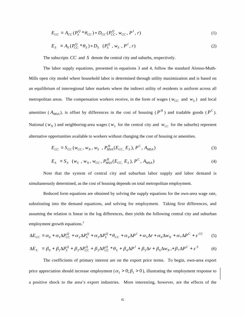
C. Measuring Exogenous Shocks to Export Industries

The urban growth literature on central city-suburb interactions is hampered by an inability to

differentiate exogenous shocks to the central city economy from shocks to the suburban economy. This

inability has also prevented the agglomeration literature from examining spillover-effect between the two

8

areas. To overcome this problem, this paper uses an indicator of external demand shocks, developed in

Pennington-Cross (1997), called the Export Price Index (EPI). The EPI is a weighted price index of

goods exported from an individual metropolitan area.

While Pennington-Cross (1997) constructs this index at the metropolitan level, the EPI for the

current study is constructed separately for both central cites and suburbs. Following Pennington-Cross

(1997), the MSA export industries are identified using location quotients (LQ). The LQ is a standard tool

well established in regional economic analysis as noted in Brown, Coulson, and Engle (1992) and is

defined as the share of employment for industry i in MSA m divided by the same industry employment

share for the country.

LQ = (E E() EUS ) (10)im im Em i,US

In order to ensure that the EPI only captures shocks that are exogenous to the metropolitan area,

the location quotients are calculated for the MSA as a whole, rather than for the central city and suburbs

separately. Otherwise, local industries, trading between the central city and suburbs, would be identified

as an export industry, biasing the index with endogenous shocks between the central city and suburbs and

the results toward a positive relationship.

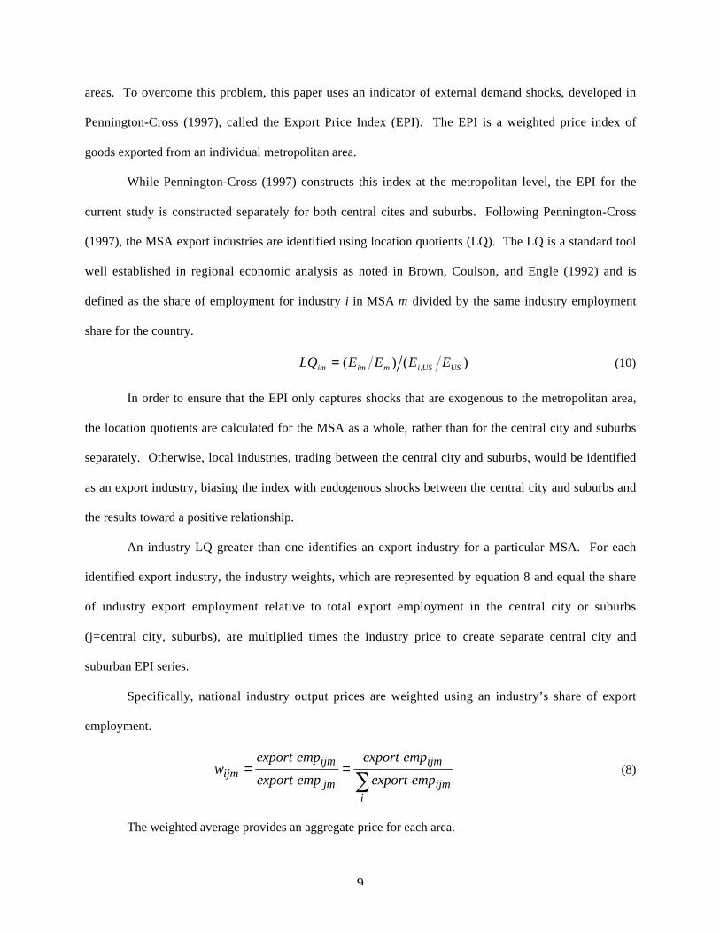
An industry LQ greater than one identifies an export industry for a particular MSA. For each

identified export industry, the industry weights, which are represented by equation 8 and equal the share

of industry export employment relative to total export employment in the central city or suburbs

(j=central city, suburbs), are multiplied times the industry price to create separate central city and

suburban EPI series.

Specifically, national industry output prices are weighted using an industry’s share of export

employment.

(8)

The weighted average provides an aggregate price for each area.

∑ ==

i ijm

ijm

jm

ijm ijm empxporte

empxporte

empxporte

empxportew

9

[P ' ][w ] = EPI (9)i ijm ijm

IV. RESULTS

Equations 5 and 6 are estimated using panel data for 77 MSAs from 1982 to 2000. Table 1 lists

the sample MSAs while Table 2 contains the variable definitions and sources. Tables 3 and 4 present the

reduced form model estimates using the two alternative measures of industrial concentration: employment

share of the three largest export industries and a Hirschman-Herfandahl index (HHI) of export

employment. The signs of the estimates agree well with prior expectations. Increases in intermediate

input price appreciation ( α 4 < 0; β4 < 0 ), national wage growth ( α < 0; β6 < 0 ) and lagged consumer 6

price appreciation ( α7 < 0; β7 < 0 ) all decrease employment, in both the central city and suburbs.

Increases in the rate of change in interest rates ( α5 > 0; β5 > 0 ) result in increased employment.

Presumably, this reflects the substitution of labor for capital. The elasticity of employment with respect

to consumer prices is negative, reflecting the higher cost-of-living in urban versus rural areas. Finally, the

own-area EPI performed as expected, capturing the effect of demand shocks implied by the positive

coefficient for both the central city and suburbs (α1 > 0; β1 > 0 ).

The neighboring-area EPI and the interaction term with industrial concentration identify the

nature of both the geographic and industrial dimensions of agglomeration economies. In both

specifications (Tables 3 and 4), the coefficient on the neighboring area EPI, representing the geographic

dimension, is positive and significant ( α 2 > 0; β2 > 0 ), indicating that a positive demand shock in one

area results in net gains in employment in the neighboring area if the neighboring area has highly

diversified export industries. Given that the positive shock increases employment and wages in the area

where it is experienced, the positive inter-area effect implies that productivity increases in the other area

are large enough to offset the effects of higher labor costs.

At high levels of industrial concentration, however, the inter-area effect not only diminishes but

also becomes negative ( α3 < 0; β < 0 ). This indicates that the positive effects found based on the 3

10

coefficient of neighboring area EPI result from the presence of urbanization economies because they

diminish and even become negative as diversity decreases. Of course, this is just the result that was

anticipated a priori, but it is gratifying to note that the indirect test performed here appears to demonstrate

that the importance of urbanization economies is so sensitive to the degree of diversification of the urban

economy.

Table 5 provides an interpretation of the results in Tables 3 and 4 for various levels of industrial

concentration. Table 6 provides the results for each MSA. The first box of each panel in Table 5

provides the results using the industry employment share measure, associated with the equations from

Table 3, and the second box corresponds to the HHI measure used in Table 4.

The top panel of Table 5 calculates the net effect of a 1% demand shock to the suburbs on central

city employment growth. For both concentration measures, the initial positive effect is offset as own-area

concentration increases, i.e. urbanization economies dominate and higher levels of specialization limit

urban growth. The net effect of the shock, evaluated at the average concentration level of 28.8%,

increases central city employment 0.1029%. This positive effect is completely offset when the three

largest export industries account for 40.1% of employment, which is less than one standard deviation

above the mean. For the maximum concentration level in the sample, 81.9% in Atlantic City,

urbanization economies are so small that a positive center city shock of 1% causes a decrease in

employment of 0.3812%. The results using the HHI measure of industrial concentration show a similar

result.

The effect of exogenous central city demand shocks on suburban employment growth, shown in

the lower panel of Table 5, is similar with one notable exception. The level of concentration at which the

shock is completely offset is much higher indicating that the suburbs have a larger growth response to

changes in central city. Evaluated at the mean concentration level, employment share of 31.0% for the

three largest export industries, a 1% central city demand shock increases suburban employment 0.3606%.

At one standard deviation above the mean, 45.4%, the effect of the shock remains strong, increasing

suburban employment 0.1782%. The shock is not completely offset until the concentration level is

11

59.6%. For the Santa Fe, NM MSA, the city with the most concentrated suburbs, 74.7% of export

employment in the three largest export industries, a 1% shock to the central city decreases suburban

employment 0.1913%. In contrast, Chicago has the most diverse suburban industrial structure; the three

largest export industries contain Thus, a 1% shock to the central city increases suburban employment

0.6109%.

V. CONCLUSION

This paper has examined the nature of agglomeration externalities at the sub-metropolitan level,

using an index of demand shocks exogenous to the metropolitan region. Theories of agglomeration

externalities contend that due to the nature of knowledge spillovers, urban growth varies with industrial

concentration and geographic proximity. Marshall (1890) posits that knowledge transfers occur primarily

between firms within the same industry and therefore growth is higher when an urban area is dominated

by one industry. Jacobs (1969) emphasizes that inter-industry interactions foster innovations and

therefore higher growth. Thus, diversity is important for the growth of a city.

Results of reduced form employment growth equations for central cities and suburbs reveal that

agglomeration externalities, in the form of urbanization economies, do exist, but that their relative

importance varies with the diversity of local industrial structure and hence that it varies across cities.. For

cities where the industrial structure is moderately diverse, the positive demand shocks to the center city

result in substantial growth in the suburbs, and vice versa. This indicates that the positive effects of

urbanization economies across sectors outweigh any tendency for growth of the “rival” area to raise

wages, congestion, and other production costs. Conversely, for cities with a specialized or concentrated

industrial structure, the effects of cross-area demand shocks are reversed. Thus, the importance of

urbanization economies appears to depend on local industrial structure. For example, in Salt Lake City’s

central city, the three largest export industries account for 15.5% of its export employment, placing it at

the top of the first decile. A positive 1% shock to the suburb economy would increase central city

employment 0.22%. At the top of the ninth decile, the three largest export industries in Memphis’s

12

central city comprise 43.3% of total central city export employment. Due to the higher concentration, or

lack of diversity, a 1.0% shock to the Memphis suburbs would decrease central city employment by

0.03%. These results explain why the current literature contains strong empirical support for the

importance of both urbanization and localization economies. Put another way, the results confirm the

findings of Glaeser et al. (1992) that industrial diversity promotes overall city employment growth but

also explain why Henderson (2001), Moomaw (1988), and Rosentahl and Strange (2003) find that

localization economies can be very important in manufacturing.

It should be emphasized that these results are based on a sample of the largest metropolitan areas

in the U.S. The smallest urban area in the sample is Sante Fe, New Mexico with 1999 population of

142,500 and 1999 employment of 65,200. All other metropolitan areas in the sample have over 200,000

residents and 100,000 jobs. Theories of agglomeration externalities, such as Henderson’s (1988) system

of cities model, generally posit that localization economies lead to small and medium-sized cities

dominated by a single export industry whereas urbanization economies are associated with larger cities.

Results presented here are in general agreement with this reasoning.

REFERENCES

Arrow, Kenneth, “The Economic Implications of Learning by Doing,” Review of Economic Studies 29 (1962), 155-173.

Brooks, Nancy and Anita Summers, “Does the Economic Health of America’s Largest Cities Affect the Economic Health of their Suburbs?,” Wharton Real Estate Center Working Paper No. 263 (1997).

Brown, Scott, Edward Coulson and Robert Engle, “On the Determination of Regional Base and Regional Base Multipliers,” Regional Science and Urban Economics 22 (1992), 619-635.

Carlino, Gerald, Chatterjee, Satyajit, and Robert Hunt. “Knowledge Spillovers and the New Economy of Cities” Working Paper No. 01-14 (2001), Federal Reserve Bank of Philadelphia.

Chinitz, Benjamin. “Contrasts in Agglomeration: New York and Pittsburgh” American Economic Review 51 (1961), 279-289.

Fujita, Masahisa, Paul Krugman, and Anthony Venables, The Spatial Economy: Cities, Regions, and International Trade (Cambridge, MA: MIT Press, 2001).

Glaeser, Edward, Hedi Kallal, Jose Scheinkman, and Andei Shleifer, “Growth in Cities,” Journal of Political Economy 100 (1992), 1126-1152.

Henderson, Vernon, “Efficiency of Resource Usage and City Size,” Journal of Urban Economics 19 (1986), 47-70.

____, Urban Development: Theory, Fact, and Illusion (New York, NY: Oxford University Press, 1988).

13

____, “Externalities and Industrial Development,” Journal of Urban Economics 42 (1997), 449-470.

____, “Marshall’s Scale Economies,” Journal of Urban Economics 53 (2003), 1-28.

Henderson, Vernon, Ari Kuncoro, and Matt Turner, “Industrial Development in Cities,” Journal of Political Economy 103 (1995), 1067-1090.

Ihlanfeldt, Keith. “The Importance of the Central City to the Regional and National Economy: A Review of the Arguments and Empirical Evidence” Cityscape: A Journal of Policy Development and Research 1 (1995), 125-150.

Jacobs, Jane, The Economy of Cities (New York, NY: Vintage, 1969).

Marshall, Alfred, Principles of Economics (London, UK: Macmillan, 1890).

Moomaw, Ronald, “Agglomeration Economies: Localization or Urbanization?,” Urban Studies 25 (1988), 150-161.

Nakamura, Ryohei. “Agglomeration Economies in Urban Manufacturing Industries: A Case of Japanese Cities” Journal of Urban Economics 17 (1985), 108-124.

Pennington-Cross, Anthony, “Measuring External Shocks to the City Economy: An Index of Export Prices and Terms of Trade,” Real Estate Economics 25 (1997), 105-128.

Romer, Paul, “Increasing Returns and Long-Run Growth,” Journal of Political Economy 94 (1986), 1002-1037.

Rosenthal, Stuart and William Strange, “Determinants of Agglomeration,” Journal of Urban Economics 50 (2001), 191-229.

____, “Geography, Industrial Organization and Agglomeration,” Review of Economics and Statistics 85 (2003), 377-393.

____, “Evidence on the Nature and Sources of Agglomeration Economies,” in Handbook for Urban and Regional Economics, Volume 4, J.V. Henderson and J.F. Thisse, eds. (New York, NY: North-Holland, 2004).

Sullivan, Arthur, “A General Equilibrium Model with External Scale Economies in Production,” Journal of Urban Economics 13 (1983), 235-255.

____, “A General Equilibrium Model with Agglomerative Economies and Decentralized Employment,” Journal of Urban Economics 20 (1986), 55-74.

Voith, Richard, “Do Suburbs Need Cities?,” Journal of Regional Science 38 (1998), 445-464.

14

Notes

1 Carlino, Chatterjee and Hunt (2001), for example, find that the rate of innovation is substantially higher in the densest urban areas.

2 Rosenthal and Strange (2004) identify three dimensions over which agglomeration externalities occur: industrial, geographic and temporal. These are discussed further in the literature review.

3 The results presented here also include MSA fixed effects. Results excluding fixed effects dummies yield similar results and are available from the author upon request.

4 See Ihanfeldt (1995) for a review of the central city/suburb literature. 5 Unlike Glaeser et al. (1992) and Henderson, Kuncoro and Turner (1995), the measures are included in

alternate specifications, rather than including both measures in the same equation.

15

TABLE 1.- MSAS IN SAMPLE

Akron, OH PMSA Lexington, KY MSA Albuquerque, NM MSA Little Rock-North Little Rock, AR MSA Ann Arbor, MI PMSA Louisville, KY-IN MSA Atlanta, GA MSA Macon, GA MSA Atlantic-Cape May, NJ PMSA Memphis, TN-AR-MS MSA Austin-San Marcos, TX MSA Milwaukee-Waukesha, WI PMSA Baltimore, MD PMSA Minneapolis-St. Paul, MN-WI MSA Baton Rouge, LA MSA Nashville, TN MSA Birmingham, AL MSA New Orleans, LA MSA Boise City, ID MSA New York, NY PMSA Buffalo-Niagara Falls, NY MSA Newark, NJ PMSA Canton-Massillon, OH MSA Norfolk-Virginia Beach-Newport News, VA-NC MSA Charleston-North Charleston, SC MSA Oakland, CA PMSA Charlotte-Gastonia-Rock Hill, NC-SC MSA Oklahoma City, OK MSA Chattanooga, TN-GA MSA Omaha, NE-IA MSA Chicago, IL PMSA Orlando, FL MSA Cincinnati, OH-KY-IN PMSA Philadelphia, PA-NJ PMSA Cleveland-Lorain-Elyria, OH PMSA Phoenix-Mesa, AZ MSA Columbia, SC MSA Pittsburgh, PA MSA Columbus, OH MSA Portland-Vancouver, OR-WA PMSA Dallas, TX PMSA Roanoke, VA MSA Daytona Beach, FL MSA Rochester, NY MSA Denver, CO PMSA Rockford, IL MSA Des Moines, IA MSA Sacramento, CA PMSA Detroit, MI PMSA Salem, OR PMSA Fort Wayne, IN MSA Salt Lake City-Ogden, UT MSA Fort Worth-Arlington, TX PMSA San Antonio, TX MSA Fresno, CA MSA San Francisco, CA PMSA Gary, IN PMSA Santa Fe, NM MSA Harrisburg-Lebanon-Carlisle, PA MSA Seattle-Bellevue-Everett, WA PMSA Houston, TX PMSA Springfield, IL MSA Huntsville, AL MSA St. Louis, MO-IL MSA Indianapolis, IN MSA Syracuse, NY MSA Jackson, MS MSA Toledo, OH MSA Jacksonville, FL MSA Tulsa, OK MSA Kansas City, MO-KS MSA Washington, DC-MD-VA-WV PMSA Knoxville, TN MSA Wichita, KS MSA Lansing-East Lansing, MI MSA Wilmington-Newark, DE-MD PMSA Las Vegas, NV-AZ MSA

16

TABLE 2.- DATA DEFINITIONS AND SOURCES

Variable Description Ej Central City, Suburb Employment (Bureau of Labor Statistics)

EPI Export Price Index (EPI) (constructed as discussed in Section IIIC) θj 1. Export employment share of the three largest export industries in area j

2. Herschman-Herfindal Index of Export Employment (calculated as discussed in Section IIIC)

PI Producer Price Index (Bureau of Labor Statistics)

r One-Year Treasury Rate (Federal Reserve Board)

wN National Average Wage (Bureau of Labor Statistics)

PC Consumer Price Index (Bureau of Labor Statistics)

Note: Employment data in BLS' Quarterly Census of Employment and Wages (QCEW) is reported on a county basis. Thus, in this study, the county in which the central city is located represents the central city while the remaining counties form the suburbs.

17

TABLE 3.- CENTRAL CITY AND SUBURB EMPLOYMENT GROWTH WITH INDUSTRY SHARE EFFECTS

variable Δ EPICC

Δ EPICC * θ S

Ind

Δ EPIS

Δ EPIS * θ CC

Ind

Δ PI

Δ r Δ wN

Δ PC

stnd error 0.3018 * 0.0504

0.3654 * 0.0906 -0.9114 * 0.2561 -0.0320 0.0231 0.0017 * 0.0003

-0.1259 * 0.0361 -0.7499 * 0.0287

Central City coefficient stnd error

0.7511 * 0.1132 -1.2612 * 0.2997 0.2934 * 0.0522

-0.1193 * 0.0277 0.0019 * 0.0004

-0.1749 * 0.0431 -0.9586 * 0.0349

Suburb coefficient

Fixed Effects MSA Dummies MSA Dummies

# MSAs 77 77 Observations 1463 1463 * = significant at 1% Confidence Level

Note: Industry concentration, θ jInd (j= CC, S), is measured using the export

employment share of the three largest export industries.

18

TABLE 4.- CENTRAL CITY AND SUBURB EMPLOYMENT GROWTH WITH HHI EFFECTS

variable Δ EPICC

Δ EPICC * θ S

HHI

Δ EPIS

Δ EPIS * θ CC

HHI

Δ PI

Δ r Δ wN

Δ PC

stnd error 0.3038 * 0.0509

0.1635 * 0.0489 -1.4835 * 0.5433 -0.0269 0.0229 0.0017 * 0.0003

-0.1285 * 0.0361 -0.7425 * 0.0286

coefficient Central City

stnd error 0.5376 * 0.0774

-2.7265 * 0.6554 0.3038 * 0.0525

-0.1173 * 0.0277 0.0019 * 0.0004

-0.1718 * 0.0431 -0.9560 * 0.0348

coefficient Suburb

Fixed Effects MSA Dummies MSA Dummies

# MSAs 77 77 Observations 1463 1463 * = significant at 1% Confidence Level

Note: Industry concentration, θ jHHI (j= CC, S), is measured using a

Herschman-Herfindal Index of Export Employment (see Section IIIB).

19

TABLE 5.- NET EFFECT OF EXOGENOUS DEMAND SHOCKS

Effect of 1% Shock to Suburb on Central City Employment

Δ EPIS

coefficient Δ EPIS

coefficient

Δ EPIS * θ CC

Ind -0.9114

0.3654 Δ EPIS * θ

CC HHI

-1.4835

θ CC

Ind evaluated at:

minimum mean shock completely offset 1 s.d above mean maximum

11.7% 28.8% 40.1% 42.4% 81.9%

1% Shock Net Effect of

0.2590 0.1029 0.0000

-0.0208

θ CC

HHI evaluated at:

minimum mean shock completely offset 1 s.d above mean

0.1635

0.013 0.061 0.110 0.155

1% Shock Net Effect of

0.1447 0.0727 0.0000

-0.0667

Effect of 1% Shock to Central City on Suburb Employment

-0.3812 maximum 0.622 -0.7599

Δ EPICC

coefficient Δ EPICC

coefficient

Δ EPICC * θ S

Ind -1.2612

0.7511 Δ EPICC * θ

S HHI

-2.7265

0.5376

θ S

Ind evaluated at:

minimum 11.1% 31.0%

1% Shock Net Effect of

0.6108

θ S

HHI evaluated at:

minimum 0.011 0.068

1% Shock Net Effect of

0.5070

1 s.d above mean mean

45.4% 0.1782 0.3606

1 s.d above mean mean

0.139 0.1591 0.3516

shock completely offset maximum

59.6% 74.7%

0.0000 -0.1913

shock completely offset maximum

0.197 0.364

0.0000 -0.4541

20

TABLE 6.- NET EFFECT OF EXOGENOUS DEMAND SHOCKS BY MSA

MSA Name θ CC

Ind

Net Effect of 1% Shock to

Suburbs θ CC

HHI

Net Effect of 1% Shock to

Suburbs θ S

Ind

Net Effect of 1% Shock to

CC θ S

HHI

Net Effect of 1% Shock to

CC

Akron, OH 19.1% 0.1910 0.0255 0.1257 21.1% 0.4848 0.0326 0.4487 Albuquerque, NM 25.2% 0.1355 0.0371 0.1085 62.3% -0.0345 0.2798 -0.2252 Ann Arbor, MI 37.9% 0.0197 0.0797 0.0453 32.6% 0.3399 0.0619 0.3688 Atlanta, GA 25.2% 0.1356 0.0309 0.1176 21.1% 0.4847 0.0247 0.4702 Atlantic-Cape May, NJ 81.9% -0.3812 0.6225 -0.7599 40.7% 0.2374 0.0827 0.3122 Austin-San Marcos, TX 35.6% 0.0406 0.0577 0.0779 46.6% 0.1635 0.1280 0.1886 Baltimore, MD 32.2% 0.0720 0.0506 0.0884 13.6% 0.5790 0.0165 0.4927 Baton Rouge, LA 17.4% 0.2067 0.0234 0.1287 26.9% 0.4113 0.0422 0.4225 Birmingham, AL 15.9% 0.2208 0.0195 0.1345 12.9% 0.5887 0.0190 0.4858 Boise City, ID 44.6% -0.0412 0.0989 0.0167 32.8% 0.3375 0.0515 0.3973 Buffalo-Niagara Falls, NY 14.9% 0.2300 0.0176 0.1374 32.5% 0.3409 0.0649 0.3608 Canton-Massillon, OH 22.5% 0.1608 0.0291 0.1203 60.2% -0.0078 0.2320 -0.0950 Charleston-North Charleston, SC 28.6% 0.1051 0.0418 0.1015 28.0% 0.3979 0.0440 0.4177 Charlotte-Gastonia-Rock Hill, NC-SC 22.8% 0.1575 0.0318 0.1163 23.2% 0.4586 0.0320 0.4503 Chattanooga, TN-GA 33.9% 0.0568 0.0654 0.0664 46.0% 0.1706 0.0944 0.2803 Chicago, IL 11.7% 0.2590 0.0127 0.1447 11.1% 0.6108 0.0112 0.5070 Cincinnati, OH-KY-IN 23.9% 0.1473 0.0305 0.1182 19.0% 0.5118 0.0240 0.4723 Cleveland-Lorain-Elyria, OH 16.7% 0.2129 0.0196 0.1344 12.6% 0.5920 0.0170 0.4913 Columbia, SC 19.1% 0.1915 0.0278 0.1222 18.1% 0.5226 0.0264 0.4656 Columbus, OH 18.3% 0.1987 0.0228 0.1297 27.9% 0.3995 0.0404 0.4274 Dallas, TX 14.3% 0.2353 0.0173 0.1378 23.4% 0.4565 0.0310 0.4532 Daytona Beach, FL 25.3% 0.1347 0.0355 0.1108 31.9% 0.3494 0.0562 0.3844 Denver, CO 27.5% 0.1145 0.0389 0.1058 20.7% 0.4904 0.0252 0.4690 Des Moines, IA 27.6% 0.1142 0.0436 0.0988 39.6% 0.2522 0.0751 0.3329 Detroit, MI 48.0% -0.0717 0.1074 0.0041 35.1% 0.3085 0.0624 0.3674 Fort Wayne, IN 21.7% 0.1673 0.0299 0.1192 19.6% 0.5034 0.0295 0.4573 Fort Worth-Arlington, TX 39.6% 0.0042 0.0711 0.0580 23.2% 0.4579 0.0336 0.4461 Fresno, CA 42.7% -0.0235 0.1006 0.0142 62.9% -0.0420 0.1875 0.0265 Gary, IN 49.6% -0.0862 0.1331 -0.0340 61.7% -0.0270 0.2896 -0.2520 Harrisburg-Lebanon-Carlisle, PA 31.2% 0.0811 0.0471 0.0936 29.6% 0.3773 0.0439 0.4180 Houston, TX 20.3% 0.1800 0.0259 0.1251 18.8% 0.5142 0.0248 0.4700 Huntsville, AL 33.2% 0.0630 0.0546 0.0824 58.9% 0.0078 0.2065 -0.0254 Indianapolis, IN 17.2% 0.2089 0.0219 0.1309 19.4% 0.5067 0.0279 0.4616 Jackson, MS 20.4% 0.1799 0.0322 0.1156 22.8% 0.4641 0.0372 0.4363 Jacksonville, FL 20.7% 0.1764 0.0317 0.1164 30.6% 0.3646 0.0467 0.4104 Kansas City, MO-KS 28.0% 0.1102 0.0383 0.1066 23.7% 0.4518 0.0304 0.4546 Knoxville, TN 19.5% 0.1876 0.0257 0.1253 21.3% 0.4822 0.0332 0.4470 Lansing-East Lansing, MI 42.5% -0.0223 0.1017 0.0127 25.9% 0.4246 0.0393 0.4305 Las Vegas, NV-AZ 80.4% -0.3669 0.5720 -0.6851 51.7% 0.0988 0.1119 0.2325 Lexington, KY 29.2% 0.0989 0.0485 0.0915 34.9% 0.3110 0.0771 0.3274 Little Rock-North Little Rock, AR 20.6% 0.1779 0.0260 0.1249 27.2% 0.4083 0.0425 0.4219 Louisville, KY-IN 27.3% 0.1170 0.0409 0.1028 23.0% 0.4612 0.0333 0.4469 Macon, GA 32.5% 0.0688 0.0506 0.0884 26.1% 0.4219 0.0431 0.4200 Memphis, TN-AR-MS 43.3% -0.0296 0.0947 0.0229 25.0% 0.4352 0.0367 0.4377 Milwaukee-Waukesha, WI 13.4% 0.2429 0.0160 0.1398 16.0% 0.5487 0.0203 0.4824 Minneapolis-St. Paul, MN-WI 16.3% 0.2173 0.0193 0.1348 17.0% 0.5366 0.0206 0.4816 Nashville, TN 20.9% 0.1751 0.0271 0.1232 18.8% 0.5141 0.0233 0.4740 New Orleans, LA 27.4% 0.1160 0.0386 0.1062 24.9% 0.4374 0.0343 0.4442 New York, NY 22.6% 0.1591 0.0301 0.1189 15.4% 0.5563 0.0212 0.4799 Newark, NJ 25.1% 0.1365 0.0347 0.1120 20.2% 0.4964 0.0242 0.4716 Norfolk-Virginia Beach-Newport News, VA-NC 26.0% 0.1285 0.0368 0.1089 31.4% 0.3552 0.0515 0.3972 Oakland, CA 12.2% 0.2545 0.0139 0.1429 24.9% 0.4375 0.0321 0.4500 Oklahoma City, OK 18.8% 0.1941 0.0256 0.1255 22.1% 0.4719 0.0317 0.4513 Omaha, NE-IA 31.5% 0.0781 0.0454 0.0961 51.8% 0.0980 0.1531 0.1201 Orlando, FL 54.3% -0.1293 0.1369 -0.0396 29.5% 0.3793 0.0511 0.3983 Philadelphia, PA-NJ 37.3% 0.0251 0.0671 0.0639 17.2% 0.5346 0.0189 0.4860 Phoenix-Mesa, AZ 33.7% 0.0587 0.0549 0.0820 59.1% 0.0057 0.1972 0.0000 Pittsburgh, PA 27.4% 0.1153 0.0400 0.1042 20.2% 0.4959 0.0248 0.4699 Portland-Vancouver, OR-WA 13.0% 0.2472 0.0142 0.1424 25.1% 0.4352 0.0401 0.4283 Roanoke, VA 26.8% 0.1211 0.0357 0.1105 27.0% 0.4108 0.0419 0.4234 Rochester, NY 47.5% -0.0677 0.1424 -0.0478 19.1% 0.5102 0.0273 0.4631 Rockford, IL 23.9% 0.1474 0.0326 0.1151 41.7% 0.2257 0.0998 0.2656

21

NET EFFECT OF EXOGENOUS DEMAND SHOCKS BY MSA (CONTINUED)

MSA Name θ CC

Ind

Net Effect of 1% Shock to

Suburbs θ CC

HHI

Net Effect of 1% Shock to

Suburbs θ S

Ind

Net Effect of 1% Shock to

CC θ S

HHI

Net Effect of 1% Shock to

CC

Sacramento, CA 14.7% 0.2318 0.0219 0.1310 30.6% 0.3650 0.0480 0.4067 St. Louis, MO-IL 25.9% 0.1291 0.0386 0.1062 22.2% 0.4705 0.0287 0.4593 Salem, OR 19.2% 0.1904 0.0271 0.1232 33.9% 0.3235 0.0651 0.3603 Salt Lake City-Ogden, UT 15.5% 0.2245 0.0189 0.1354 16.3% 0.5449 0.0206 0.4814 San Antonio, TX 26.1% 0.1277 0.0345 0.1123 31.2% 0.3579 0.0546 0.3889 San Francisco, CA 19.7% 0.1861 0.0250 0.1263 30.0% 0.3725 0.0440 0.4177 Santa Fe, NM 33.9% 0.0560 0.0502 0.0889 74.7% -0.1913 0.2478 -0.1380 Seattle-Bellevue-Everett, WA 38.4% 0.0159 0.0760 0.0507 67.9% -0.1057 0.3637 -0.4541 Springfield, IL 32.8% 0.0661 0.0575 0.0782 43.2% 0.2067 0.0936 0.2824 Syracuse, NY 19.8% 0.1851 0.0258 0.1253 19.2% 0.5094 0.0281 0.4610 Toledo, OH 28.3% 0.1077 0.0373 0.1081 35.1% 0.3080 0.0532 0.3927 Tulsa, OK 21.5% 0.1699 0.0295 0.1197 35.5% 0.3029 0.0628 0.3663 Washington, DC-MD-VA-WV 29.0% 0.1014 0.0475 0.0930 23.3% 0.4573 0.0333 0.4468 Wichita, KS 66.1% -0.2374 0.2075 -0.1444 41.9% 0.2220 0.1029 0.2570 Wilmington-Newark, DE-MD 38.7% 0.0130 0.0679 0.0627 51.5% 0.1015 0.1447 0.1432

22