Distance from Urban Agglomeration Economies and Rural Poverty

by

Mark D. Partridge C. William Swank Chair in Rural-Urban Policy

Professor, Department of Agricultural, Environmental, and Development Economics Ohio State University

2120 Fyffe Road Columbus, OH 43210, USA

Phone: 306-966-4037; Fax: 614-688-3622 Email: partridge.27@osu.edu, Webpage: http://aede.osu.edu/programs/Swank/

and

Dan S. Rickman OG&E Chair in Regional Economic Analysis

Professor of Economics 338 College of Business

Oklahoma State University Stillwater, OK 74078

Phone: 405-744-1434, Fax: 405-744-5180 Email: dan.rickman@okstate.edu

May 24, 2007

Abstract

Despite strong growth during the 1990s economic expansion being accompanied by significant reductions

in measures of U.S. poverty, high poverty persisted in remote rural areas. Therefore, this study uses a

novel geographical information system database of county-urban proximity measures to examine the

nexus between poverty in rural U.S. counties and their remoteness, particularly in regard to their

geographical proximity to larger urban centers. We find that poverty rates are positively associated with

greater rural distances from successively larger (higher-tiered) metropolitan areas (ceteris paribus). We

explain this outcome as arising from the attenuation of urban agglomeration effects at greater distances

and incomplete labor supply adjustments in remote rural areas in the form of commuting and migration.

Yet, although our results suggest that they are at a disadvantage in terms of reduced benefits from urban

agglomeration economies, remote rural areas also may particularly benefit from place-based economic

development policies in terms of their effect on poverty.

JEL: R12, I32, R23

Distance from Urban Agglomeration Economies and Rural Poverty

Abstract

Despite strong growth during the 1990s economic expansion being accompanied by significant reductions

in measures of U.S. poverty, high poverty persisted in remote rural areas. Therefore, this study uses a

novel geographical information system database of county-urban proximity measures to examine the

nexus between poverty in rural U.S. counties and their remoteness, particularly in regard to their

geographical proximity to larger urban centers. We find that poverty rates are positively associated with

greater rural distances from successively larger (higher-tiered) metropolitan areas (ceteris paribus). We

explain this outcome as arising from the attenuation of urban agglomeration effects at greater distances

and incomplete labor supply adjustments in remote rural areas in the form of commuting and migration.

Yet, although our results suggest that they are at a disadvantage in terms of reduced benefits from urban

agglomeration economies, remote rural areas also may particularly benefit from place-based economic

development policies in terms of their effect on poverty.

JEL: R12, I32, R23

1

1. Introduction

Strong U.S. macroeconomic performance during the 1990s expansion was accompanied by a

reduction in the overall person poverty rate from 15.1 percent in 1993 to 11.3 percent in 2000, bringing it

to the lowest level since 1974 (U.S. Census Bureau, 2006).1 The apparent strong link between economic

growth and poverty reduction was notable given its weakening during the 1980s (Freeman, 2001).2 Yet,

poverty remains high in many areas of nonmetropolitan America, particularly in counties non-adjacent to

or far removed from metropolitan areas (Glasmeier and Farrigan, 2003; Swaminathan and Findeis, 2004;

Partridge and Rickman, 2006, Ch. 2).

An extensive literature has emerged examining whether there is a rural poverty effect. 3 For

example, Gibbs (1994) and Davis and Weber (2002) argue that rural labor markets are thinner with poorer

employer-employee matches than their urban counterparts, while Henry, Barkley and Bao (1997) describe

other remote-rural barriers to development. Levernier, Partridge and Rickman (2000) find higher poverty

in U.S. nonmetropolitan counties that is not accounted for by industrial structure or demographic

characteristics. But is poverty higher in these rural areas because of their remoteness, or because of other

factors such as natural amenities or the demographic composition of the local population? In their survey,

although Weber et al. (2005) conclude that poverty is higher and more persistent in the more remote rural

counties, they were reluctant to describe this as a rural effect. Fisher (2005; 2007) shows that while part of

the higher rate of poverty in rural areas is attributable to poor economic opportunities, she also contends

that part is attributable to self-selection of poor people into rural areas.

Despite the emphasis on distance in New Economic Geography models and regional economics

in general, to the best of our knowledge there have not been any studies that have empirically assessed the

nexus between poverty in rural areas and their geographic proximity in the urban hierarchy. Distance can

1In analyses of state poverty rate trends, Gundersen and Ziliak (2004) and Partridge and Rickman (2006, Ch. 4)

concluded that it was strong economic performance that primarily reduced poverty in the late 1990s, not welfare reform.

2Although the link between strength in the labor market and the poverty rate over the entire 1990-2003 period

was comparable to the weakened link in the 1980s (Hoynes, Page and Stevens, 2006), the link dramatically

strengthened in the late 1990s as the expansion lengthened and the labor market became tighter (Hines, Hoynes and

Krueger, 2001; Partridge and Rickman, 2006, pp. 91-95). 3Since official poverty rates are not adjusted for regional cost-of-living differentials, there has been considerable

speculation on whether lower prices in nonmetropolitan areas, particularly for housing, equalize real poverty rates across nonmetropolitan and metropolitan areas. Nevertheless, the U.S. General Accounting Office (1995) has concluded there is insufficient official data to geographically adjust poverty rates for price. Moreover, costs of food and other items such as transportation could be higher in the most remote rural areas because of delivery costs and distance, offsetting housing cost advantages (Nord and Leibtag, 2005).

2

affect poverty through influencing both rural labor demand and supply. Shorter distances between firms

yield many economic advantages for metropolitan areas, leading to agglomeration of economic activity

(for a survey see Rosenthal and Strange, 2001), and hence higher wages. Yet, the wage effects associated

with agglomeration attenuate with distance from the core area (Hanson, 1997; 1998; 2005). Distance also

appears to be a key factor underlying employment and population growth in nonmetropolitan counties.

Those adjacent to metropolitan areas grew fastest during the 1990s (USDA, 2006), and ceteris paribus,

the greater the distance from larger urban core areas, the lower was nonmetropolitan growth during this

period (Partridge et al., 2006; forthcoming). Moreover, Partridge, Bollman, Olfert, and Alasia (2007) find

that favorable growth effects in nearby urban areas spill over for about 180kms into the countryside.

Despite apparent weaker labor demand in remote rural areas, offsetting out-migration of labor

from rural areas could raise rural wages and reduce rural poverty. These equilibrium adjustments would

make long-run poverty more a function of household characteristics (Ravallion and Wodon, 1999). Yet

distance also can limit labor mobility by raising the costs of commuting and migration, which produces

higher poverty in remote areas experiencing reductions in labor demand. Distance can reduce labor

mobility because of associated information and relocation costs, both pecuniary and non-pecuniary.

Furthermore, if these costs lead to longer residence durations in rural areas, they can dynamically increase

relocation costs through increasing ties to the area, creating inertia effects (Molho, 1995). The lower long-

run labor supply elasticity due to remoteness suggests that limitations on rural-household access to good-

paying (urban) jobs can create a rural spatial-skills mismatch that is akin to inner-city spatial mismatch

outcomes that predominate the urban literature (Blumenberg and Shiki, 2004). Nevertheless, despite very

high poverty rates in many nonmetropolitan areas, there has been remarkably little examination of spatial

location and rural poverty.

Therefore, this paper empirically examines the relationship between nonmetropolitan poverty

rates and distance from metropolitan areas. A key contribution of our study is the construction of a large

geographical information system database of urban proximity measures for each U.S. county. This allows

us to estimate the poverty effects of nonmetropolitan county distances from successively higher-tiered

(larger) metropolitan areas, which to our knowledge, has never been explored in past research. If

economic activity continues to concentrate in and near the larger urban areas, then a county’s labor

3

demand growth should be inversely related to its distance from successively higher-level urban tiers. And

to the extent nonmetropolitan labor supply responses are not offsetting, poverty rates would be expected,

ceteris paribus, to be positively associated with increased distance from each higher-ordered urban tier.

The next section more formally derives the link between nonmetropolitan poverty and distance

from metropolitan agglomeration economies. The empirical model and implementation follow in Section

3. Section 4 presents the results. We find that poverty increases with greater distance from each

successive tier of metropolitan area, even when accounting for a host of county characteristics such as the

area’s amenity attractiveness and the demographic composition of the local population. Further analysis

details how rural communities receive fewer benefits from nearby metropolitan area job growth if they

are more distant. We find evidence that more remote rural communities have more inelastic labor supply,

which causes them to have higher poverty when labor demand is weaker, but allows them to capture more

poverty-reducing benefits if they were to have stronger local job growth. The final section provides a

summary and offers policy recommendations. The same accessibility factors that give rise to the distance

effect on poverty imply that employment growth has greater antipoverty effects in more remote areas. We

thus describe some reasons for place-based antipoverty policies and offer suggestions in their design.

2. Poverty and Distance from Metropolitan Areas

Area aggregate poverty rates derive from both economic and non-economic factors. Among

economic factors, the poverty rate in an area (pov) has been significantly linked to labor income, which is

given by the area’s employment rate among working age adults (er) and the associated distribution of area

wage rates (wr). 4 Thus, we express the area poverty rate as:

(1) pov = fp(er,wr,•),

where • denotes all other factors, which include non-economic factors such as the area’s demographic

characteristics. The roles of these other factors have been explored extensively in previous studies so we

leave discussion of their expected poverty effects to the next section. The employment and wage rates can

be thought of as full-time employment equivalents.

The employment and wage rate distribution are reduced-form outcomes from the interaction of

labor demand (ld) and labor supply (l

s) (Partridge and Rickman, 2003):

4For a review of the literature on the link between regional labor market outcomes and poverty, see Partridge and

Rickman (2006, Chapter 4).

4

(2) er = fer(l

d, l

s)

(3) wr = fwr

(ld, l

s),

where the labor market outcomes for the lesser skilled and educated are paramount in the determination of

the poverty rate.

Labor demand derives from location optimizing decisions by firms, which depend on a myriad of

revenue and cost considerations related to distance. If metropolitan areas are associated with

agglomeration economies, greater distance from them may negatively affect profits and labor demand in

nonmetropolitan areas, depressing their employment and shifting their wage distribution to the left,

resulting in increased poverty rates. Various theories have emerged to explain agglomeration of economic

activity.

From New Economic Geography, for example, close proximity of urban firms to their intermediate

input suppliers (i.e., input-output linkages) and customers lowers their transportation costs (Venables,

1996), causing firms to agglomerate. Costly transportation then disadvantages areas more distant from

metropolitan areas. Transactions costs such as costly information about demand conditions and

trustworthy suppliers also increase with remoteness, inhibiting trade (Hanson, 1998; 2005). Larger

agglomerated areas also offer more specialized services such as high-end business consulting or

convenient and less expensive air transportation. Other sources of agglomeration can occur through

knowledge spillovers between firms and labor-market pooling (Rosenthal and Strange, 2001). Likewise,

greater distance from metropolitan areas also may limit work-commuting opportunities in

nonmetropolitan areas (Partridge, Olfert and Alasia, 2007) and access to credit (Bigman and Fofack,

2000). Yet, forces limiting agglomeration include increased price competition associated with close

proximity of economic activity (Krugman, 1993), and congestion costs, such as higher crime, pollution,

and land prices (Glaeser, 1997). Location in remote locations could also be profitable for firms where

agglomeration economies are of less importance and low labor costs and land prices are more important.

Numerous studies have established the geographical reach of agglomeration economies. Some

effects appear to attenuate rather quickly, but not all effects. For example, knowledge externalities may

attenuate quickly because of its reliance on personal interactions, but the benefits of labor market pooling

5

and shared inputs may extend over wider areas such as U.S. states (Rosenthal and Strange, 2001; 2003).5

Likewise, Hanson (1998; 2005) finds that New Economic Geography market-potential effects diminish

with distance, but do not entirely dissipate until about 800 kms. Partridge et al. (2006; forthcoming) also

find that a U.S. county’s job growth is inversely associated with how remote it is from its higher-tiered

cities in the urban hierarchy. Agglomeration economies also are reported to extend out hundreds of kms

from major Canadian urban centers (Partridge, Olfert and Alasia, 2007), while Partridge, Bollman, Olfert,

and Alasia (2007) find agglomeration spillovers and labor market spread effects (through commuting)

that extend out about 180kms from even smaller urban centers. Finally, Dekle and Eaton (1999) find

manufacturing agglomeration effects that diminish with distance but spread nationwide in Japan.6

Even if distance creates inequality in labor demand, fully mobile households would arbitrage away

distance-based differentials in labor earnings (assuming homogeneous household preferences regarding

residential location), making labor supply perfectly elastic. Out-migration of non-employed (or under-

employed) nonmetropolitan households would increase employment and wage rates among those

remaining, reducing poverty. However, distance may affect how much labor supply responds to

metropolitan-nonmetropolitan labor demand differentials.

Information costs regarding job opportunities increase with distance (Lucas, 2001). Rural

households then may only search in labor markets with similarities to the origin market (Gibbs, 1994),

which likely precludes them from searching in urban areas. Besides similarity in labor markets, poor rural

households also may only move to other poor rural areas because of cultural similarities, the availability

of support networks, and low housing costs (Nord, 1998). Molho (1995) argues that the lower out-

migration that arises from greater remoteness leads to longer residence durations in rural areas, which

then creates cumulative inertia effects such as the building of more friendships, further limiting out-

migration. Henderson and Wang (2005) formally model differential wealth holdings in agriculture and

differential skill endowments as limiting rural out migration. If high-skilled labor is complementary with

low-skilled labor in production, out-migration of high-skilled rural labor further depresses low-skilled

5Rosenthal and Strange (2005) find evidence that even knowledge spillovers affect productivity up to 50 to 100

miles. 6In addition, van Soest, Gerking and van Oort (2006) found very localized effects for the Netherlands for services,

but their results are generally consistent with Dekle and Eaton (1999) for manufacturing.

6

wage rates, particularly if low-skilled rural laborers do not obtain the necessary training and education to

replace those departing (Lucas, 2001).

Distances also can reduce commuting to urban areas, while relocating from rural areas to more

distant urban centers with more plentiful jobs entails high relocation costs, which eliminates or greatly

reduces any net-utility gains from relocation. Thus, poverty can increase or remain stubbornly high when

resource-based sectors face persistent decline. The more inelastic labor supply that results from limited

commuting and migration flows then makes poor rural residents more dependent on local jobs. In terms

of labor supply responses, the upside of more inelastic labor supply is that if job growth were to occur in a

remote rural area, it more likely “trickles down” to the original local residents (Bartik, 1993), reducing

poverty. To rephrase, in the (less likely) case of remote areas experiencing faster growth, the distance

from other population centers would “protect” the original residents from in-commuters and in-migrants

from elsewhere.

Therefore, we express both nonmetropolitan labor demand and labor supply as dependent on an

area’s distance from metropolitan areas:

(4) ld=f

ld(dist, •), f

lddist< 0,

(5) ls = f

ls(dist, •), f

lsdist> 0 or < 0.

The net negative influence of distance on labor demand reflects the lack of access to urban agglomeration

economies (or urban productivity effects). The net influence of distance on labor supply is theoretically

ambiguous, though we hypothesized above that local labor supply is more inelastic in remote areas. Thus,

through the effects of distance on labor market outcomes, poverty rates in nonmetropolitan areas are

indirectly related to their distances from metropolitan areas:

(6) pov= fpov

(dist, •), fpov

dist> 0.

In equation (6), dist positively affects nonmetro poverty because (net) agglomeration economies attenuate

with distance from metropolitan areas, and labor supply responses by poor nonmetropolitan households to

differentials in labor demand are increasingly incomplete with greater distance causing labor supply to be

increasingly more inelastic.7

The result is a form of spatial mismatch in nonmetropolitan areas (Blumenberg and Shiki, 2004)

7The positive distance effect on poverty is based on the assumption that distance decreases labor demand more

than it could possibly reduce labor supply, reducing employment and wage opportunities for original residents.

7

akin to urban spatial mismatch, in which there are problems of geographic accessibility to best-matching

jobs for low-income households. The two cases differ because the discrimination in hiring and housing

which underlie urban spatial mismatch are likely less prevalent in rural areas. Yet, many rural areas

appear to possess the necessary and sufficient conditions for spatial mismatch, which relate to imperfect

mobility of firms and households and nontrivial search and commuting costs.8 Combined with production

being less profitable in rural areas (net of factor costs), a lack of affordable housing may constrain the

relocation of rural households to urban areas, while information and transportation costs also increase

with rural remoteness, constraining labor supply adjustment. The causal mechanisms also have some

commonality with those underlying rural poverty traps in developing countries (e.g., Lucas, 2001).

3. Empirical Implementation

The primary innovations in our empirical specification are accounting for nonmetropolitan location

within the urban hierarchy and other rural-urban interactions that can affect rural poverty outcomes. Yet,

our fully-specified (base) model is consistent with specifications found in prior spatial studies of overall

poverty rates (Madden, 1996; Levernier, Partridge and Rickman, 2000; Gundersen and Ziliak, 2004;

Partridge and Rickman, 2005). Although parsimonious models are considered, our fully-specified model

accounts for other factors that affect poverty such as the region’s demographic characteristics. A partial

(disequilibrium) adjustment formulation allows for the possibility that poverty responds sluggishly to

changes in socioeconomic conditions, making current poverty related to past poverty.

Each county has its own equilibrium (expected) poverty rate given its characteristics. Changes over

time in the underlying attributes of the area shift the equilibrium poverty rate as do local economic

shocks. Given the prevalence of economic and demographic shocks and the likelihood it may take time

for the labor market to fully respond to shocks, it is unlikely that a region’s actual poverty rate generally

equals its equilibrium rate. Thus, the current poverty rate is a function of its characteristics that determine

the expected poverty rate, current/recent economic conditions, and the lagged poverty rate to account for

disequilibrium adjustment. A significant coefficient for the lagged poverty rate suggests a slow

adjustment to shocks, making poverty rates autoregressive. An insignificant coefficient indicates a rapid

8Johnson (2006) describes the conditions for spatial mismatch in more detail. Confirming the independent role

space can play, urban spatial mismatch also has been reported for whites in Britain and the U.S. (Houston, 2005).

8

adjustment process. Accounting for the lagged poverty rate also helps control for any “fixed effects” that

persistently lead to a high or low county poverty rate.

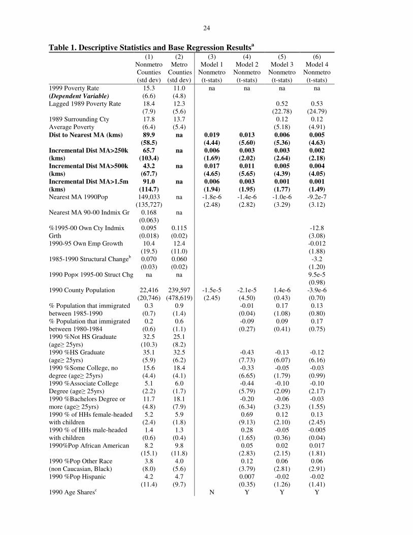
Table 1 lists the variables used in the empirical model. The dependent variable is the overall 1999

county person poverty rate.9 Most of the causal variables are generally self-explanatory, in which much of

our attention will be on the urban proximity and related urban spillover variables. Except for the job

growth variables, the values of the base model’s explanatory variables are measured around 1990 or

before to form “deep lags.” We assume that initial/current conditions in the local region determine its

long-run expected (equilibrium) poverty rate. A key advantage of controlling for lagged (pre-determined)

conditions such as demographics is it should greatly mitigate any simultaneous causality with current

poverty rates, though it may affect the statistical significance of the control variables. In sensitivity

analysis of our key urban distance results, we assess whether endogeneity is affecting the results by

initially considering parsimonious models that only include variables that are predetermined and then

successively add variables that may be less likely to be predetermined. Then we consider models that use

contemporaneous values of the explanatory variables measured around the year 2000. This extensive

analysis shows that our distance results are consistently economically meaningful and statistically

significant, suggesting that possible endogeneity or multicollinearity are not behind these findings.

Forming our base model, the following is the most complete specification of our empirical model,

which is estimated for nonmetropolitan counties (county i in state s):

(7) POVis1999= αPOVis1989 + θAVGNEIGBORPOV is1989 + δPROXIMITYis + φECONis1990s +

βCTY_TYPEis+ γDEMOGis1990 + σs + εis1999.

For the explanatory factors, AVGNEIGHBOR is the average 1989 poverty rate in contiguous counties

(includes all counties in its derivation including neighboring metropolitan and nonmetropolitan counties),

which helps pick up spatial spillover/clustering effects transmitted over time.

Reflecting the key variables of interest, the PROXIMITY vector includes measures of the county’s

proximity within the urban hierarchy as well as urban spillovers. For this study, an urban center is defined as

9Poverty rates are defined by the U.S. Census Bureau definition. Unless otherwise indicated, the variables are

drawn from Census 1990 and Census 2000 SF3 files available online at www.census.gov at American Fact Finder. One exception is the distance variables, which are derived using geographical information systems.

9

a metropolitan area (MA).10

Thus, the first measure is distance to the nearest urban center of any size, which

is measured as the distance from the county’s centroid to the centroid of the nearest MA.11

This variable

reflects a variety of access penalties. First, distance reflects the cost to access urban jobs (Henry, Barkley

and Bao, 1997; Henry, Schmitt and Piguet, 2001; Partridge, Olfert and Alasia, 2007). For low-income

workers (and other rural workers), urban areas likely have a greater diversity of jobs that yield better

employment matches and higher wages. Second, close access to urban centers improves the economic

vitality of proximate rural communities. Local economic prospects are heightened because urban customers

are nearby and closer access strengthens input-output linkages with the urban center (including through

lower transportation costs).

We include the incremental distances to more populous higher-tiered urban centers to reflect the

additional net effect of “penalties” or “protection” from being more distant from cities further up the

hierarchy. For example, greater remoteness from larger cities could inhibit rural growth due to less access to

higher-order urban services and amenities. On the other hand, spatial competition from large urban centers

may limit growth in nearby communities, which are referred to as agglomeration growth shadows in the

New Economic Geography literature (Fujita, Krugman and Mori, 1999).

To reflect these effects, we include the incremental distance in kilometers from the rural county to

reach a MA with population of at least 250,000, which may be zero kms if the nearest MA is already over

250,000.12

We also include the corresponding incremental distance to reach a metropolitan area of at least

500,000 and at least 1.5 million.13

Reflecting agglomeration and congestion effects for both firms and

households, the thresholds are consistent with those of Overman and Ioannides (2001). The largest category

10

Beginning in 2003, nonmetropolitan counties were classified as part of micropolitan areas by the Census Bureau if they had “cities” of 10,000-49,999 population or tight commuting linkages to the city. The other nonmetropolitan counties are classified as non-core-based statistical areas. We do not distinguish between them in our analysis. To see a map illustrating the location of these urban centers compared to nonmetropolitan counties, see http://www.census.gov/geo/www/maps/msa_maps2003/msa2003_previews_htm/cbsa_us_wall_0603_orig.htm.

11The population-weighted county centroids are from the U.S. Census Bureau. They were also used to derive the

population-weighted center of multi-county MAs. The MA size categories are determined by the 1990 population. 12

For example, if a rural county is 50kms from the nearest MA of (say) 100,000 population and 120kms to a MA of 300,000, the incremental distance to the nearest MA of at least 250,000 would be 70kms (120-50).

13Incremental distance is calculated as before. If the county is already nearest to a MA that is either larger than or

equal to its own size classification, then the incremental value is zero. For example, if the county’s nearest urban center of any size (or MA of any size) is already over 500,000, then the incremental values for the at-least 250,000 and at-least 500,000 categories are both equal to zero. To take another example, suppose rural county A is 30kms from its nearest MA, which has 100,000 residents, 80kms from its nearest MA >250,000 people (say 400,000 population), 200kms from a MA >500,000 (which happens to be 3 million). Then the incremental distances are 50kms to the nearest MA>250,000 (80-30), 120 incremental kms to the nearest MA>500,000 (200-80), and 0 incremental kms to a MA >1.5million (200-200).

10

generally corresponds to national and top-tier regional centers, with the 500,000-1.5 million category

reflecting sub-regional tiers. The smaller-size thresholds reflect different-size labor markets (for commuting)

and varying access to personal and business services. Although measuring distances based on population-

weighted centroids may produce some measurement error in actual “road” distances or access, this type of

measurement error simply serves to bias the coefficients downwards, against finding distance effects.

Other variables in the PROXIMITY vector include population of the nearest metropolitan center,

which captures additional agglomeration or dispersion of economic activity associated with marginal

changes in its population. Although urbanization economies draw resources from rural areas into the urban

core, rural areas closest to urban areas may fare better than the remote areas. For example, nearby rural

firms may benefit from greater access for commuters, thicker labor pools, and closer proximity to higher-

order inputs and markets (Henry, Barkley, and Bao, 1997; Partridge et al., 2006; Partridge, Olfert and

Alasia, 2007). Congestion effects also may cause rural areas close to large urban centers to grow as

economic activity disperses from the urban core.

The ECON vector contains measures of job growth and industry restructuring: 1990-1995 and 1995-

2000 county employment growth variables using place of work data from the U.S. Bureau of Economic

Analysis.14

One possible concern is that the 1995-2000 job growth may be endogenously determined with

1999 poverty rates (the dependent variable). To minimize any possible endogeneity, we substitute the 1995-

2000 industry mix variable from shift-share analysis as an exogenous proxy for local labor demand shifts.15

We are assuming that if a rural county has a high intensity of relatively slow-growing agriculture and natural

resource industries in the 1990s—i.e., a slow industry mix growth rate—then it would be expected to have

fewer work opportunities and higher poverty rates. Moreover, because employment growth over the entire

decade is considered, we assess the degree to which prolonged job growth is necessary to ensure that

employers hire disadvantaged workers rather than other members of the labor force.

14

Theory does not provide guidance as to the timing of the linkage between job growth and poverty. Experimentation at the own-county level with various time periods revealed that five-year (e.g., 1995-2000) measures were superior to those from other periods, which were often highly insignificant. We use 10-year measures when considering growth in the nearest MA. See Partridge and Rickman (2006) for more details of how the employment data was gathered.

15Industry mix employment growth is the sum of the county’s initial industry employment shares multiplied by

the corresponding national industry growth rates over the subsequent period. Because national industry growth should be exogenous to industry growth in a given county, it is routinely used as an instrument for local job growth and local demand shifts (Bartik, 1991; Blanchard and Katz, 1992; Bound and Holzer, 2000). Our primary results are not affected by this choice.

11

In further analysis, we also interact the distance from the nearest MA with a measure of the own

county’s 1995-2000 industry mix job growth to examine the hypothesis that a greater proportion of local job

growth trickles down to disadvantaged original residents in more remote rural areas. Likewise, to examine

the degree to which urban job growth “trickles out” to the rural poor, we also jointly include a measure of

the MA’s job growth and its interaction with distance to the MA. This somewhat disentangles the effect of

commuting opportunities provided by urban areas from other urban proximity benefits. In addition, if these

interaction terms are significant, this would support our hypothesis that rural poverty is at least partly related

to incomplete labor supply responses that are related to distance, producing a form of rural spatial mismatch,

versus alternative hypotheses such as low-income residents preferring to reside in more remote areas.

Industry restructuring is measured as the share of employment that has shifted across sectors over the

recent period using a dissimilarity index. More restructuring is expected to increase poverty through job

dislocation and problems associated with finding comparable new work. We also interact the restructuring

variable with population to consider whether thicker labor markets are associated with better job matching

following restructuring, and hence fewer adverse poverty effects.

The CTY_TYPE vector includes the 1990 county population. Besides accounting for the possibility

of thicker labor markets with better employment matches, own population also proxies for a county’s cost of

living.16

Another possible proxy would be to use average rental values to account for housing cost

differentials, but by definition, such a variable would be endogenously determined with the share of the

population living in poverty. However, we control for the key underlying exogenous (and predetermined)

determinants of poverty including state fixed effects (described below) that account for state-level amenity

differentials and related cost-of-living differences. We also directly control for natural amenities in

sensitivity analysis.

The DEMOG vector includes demographic traits of the population commonly believed to be

potentially correlated with poverty outcomes such as racial composition, average education, recent

immigration status, single-headed household status, and age (Levernier, Partridge and Rickman, 2000). As

noted above, these variables are deep lags, measured at their 1990 levels (or 1980-1984 and 1985-1990 for

the immigration variables) to reduce the possibility of endogeneity. The education variables are the

16For example, Gyourko and Tracy (1989) found that variation in population is a strong proxy for regional

differentials in cost of living. Also see footnote 3.

12

population proportions that have completed high school, completed some college but have no degree, have

only an associate college degree, or a bachelors degree or higher. Because of its positive linkage with

employment status and wage rates, higher education attainment should be associated with lower poverty.

We expect the presence of single-headed households to increase poverty because the heads of these

households typically possess fewer job skills, and there is typically only one earner in the household

(Levernier, Partridge and Rickman, 2000). Likewise, if there are chained migration and beachhead effects, a

higher initial immigrant share may indicate larger future increases in low-skilled labor supply. To the extent

that recent immigrants have higher poverty and compete with low-skilled natives (Borjas, 2003), a higher

share of recent immigrants would increase the poverty rate.

α, θ, β, γ, and φ represent regression coefficients, whereas, σs denotes the state-fixed effect, and ε is the

error term. Because county shocks may be transmitted to nearby counties in an economic region, we also

allow for spatial clustering (or spatial autocorrelation) of the residuals that may affect the t-statistics. Using

the Stata cluster command, we assume that county residuals are correlated within their economic region,

but independent of county residuals in other regions. We use the U.S. Bureau of Economic Analysis’s 179

economic regions to denote functional economic areas.17

State fixed effects capture specific factors

common across counties in each state such as their tax, expenditure, welfare policies, and different

geographical sizes of counties across states. Thus, the regression coefficients reflect within-state variation in

the explanatory variables, while cross-state effects are subsumed into the state fixed effects. This can cause

variables that do not greatly vary within a given state to be statistically insignificant.

4. Empirical Results

In our empirical approach, we first estimate a very parsimonious model that only includes distance

variables, own-county population, and state fixed effects. We view the estimates from this model as the

upper-bound poverty effects of distance. This model is less likely to contain endogenous relationships and

its parsimony mitigates any potential multicollinearity. Then, additional county attributes are successively

added to the specification. This is done to assess robustness of the urban proximity coefficients and to

17

An alternative approach is to use standard spatial econometric approaches to account for possible spatial autocorrelation in the error terms. Yet, Partridge and Rickman (2005) report that their nonmetropolitan county poverty results were essentially the same using this approach. Note the clustering approach has the key advantage of allowing a unique spatial correlation structure within each BEA region and it does not impose a specific spillover structure on the model, both of which would be drawbacks of standard spatial econometric approaches.

13

appraise the interaction of proximity with these other county characteristics to assess whether there is

omitted variable bias. For example, distance may partly underlie employment growth differences. Thus,

the employment growth coefficient will capture some of the poverty effects of distance. Yet, if distance

and job growth are correlated but not causally linked, omitting employment growth would bias the

distance coefficients upwards. We conclude our analysis by adding other urban-proximity indicators to

test more complex labor-market hypotheses of rural-urban interactions.

The descriptive statistics for the 2204 nonmetropolitan counties and the 824 metropolitan counties

(that comprise the urban hierarchy) are respectively reported in columns (1) and (2) of Table 1. They

reveal that nonmetro poverty rates as determined by the U.S. Census Bureau were on average over 4

percentage points higher than MA poverty rates in 1999 and over 6 points higher in 1989. The typical

nonmetro county is about 90kms from the centroid of their nearest MA (shown in bold). Job growth in

MA counties for 1990-1995 and the corresponding industry mix job growth for 1995-2000 exceeded that

in nonmetro counties by two percentage points.

4.1 Base Results

Column (3) of Table 1 shows the results from the most parsimonious regression model.18

As

expected, the results suggest that nonmetropolitan county poverty rates are positively related to distances

from higher-tiered urban centers (shown in bold). The largest estimated marginal penalty per km is

distance to the nearest MA (of any size), though the estimate for access to a MA of at least 500,000

people is almost as large. A one standard deviation increase in distance from the nearest MA is associated

with a 1.1 percentage point increase in the typical nonmetro county’s poverty rate, all else constant. By

contrast, a one standard deviation increase in incremental distance to reach the three higher tiered MAs

(<250,000, <500,000, <1.5m) is associated with a corresponding 2.5 percentage point increase in the

poverty rate; a one standard deviation increase in distance to all urban tiers then is associated with a 3.6

point increase in the poverty rate. Thus, space and location is highly associated with rural poverty.

Conversely, a one-standard deviation in the population of the nearest MA is associated with only a 0.24

percentage point decrease in the typical rural county’s poverty rate, which supports the argument that

proximity to MAs is much more important than marginal changes in the size of the nearest MA.

18

Omitting the own-county population has almost an imperceptible effect on the remaining coefficients.

14

The strong influence of distance to the nearest MA might be partly explained by access to urban

labor markets (though the rural area by definition is outside the MA labor market) directly helping

disadvantaged rural families. Yet, the greater overall importance of access to even larger MAs that are

presumably beyond easy commuting distance suggests that it is the economic vitality of the rural

community that is relatively more important. That is, better access to higher-tiered urban centers spurs

growth in rural communities through stronger interregional input-output/trade linkages and ease in

obtaining urban amenities and services (Partridge et al., 2006). Thus, it appears that rather than the direct

urban labor market access for disadvantaged workers, it is the trickle-down growth effects of broader

rural access to higher-tiered urban areas that primarily reduce rural poverty. Indeed, these trickle-down

urban-growth (urban-spread) effects have also been observed in the international development literature

(Lucas, 2001).

Model 2 adds the county’s demographic variables to the model. In this case, the PROXIMITY

coefficients are smaller in magnitude, though still statistically significant (at the 10% level or better). For

example, the proximity to the nearest MA coefficient is about one-third smaller than in Model 1.

Generally, this pattern suggests that more remote rural counties have demographic characteristics that are

associated with higher poverty rates—though it is unclear whether proximity to the urban center directly

causes demographic self-sorting, or whether other factors are behind this demographic spatial distribution.

Model 3 adds the lagged 1989 own and average-surrounding county poverty rates. Although the

urban proximity variables are still significant at the 10% level, the magnitude of their coefficients

generally decline even more between Models 2 and 3 than between Models 1 and 2. For example, the

coefficient on distance to the nearest MA declines by over one-half in Model 3. This implies that the

PROXIMITY variables are strongly correlated with lagged poverty rates. This correlation likely relates

to the general persistence of long-term county poverty rates including the underlying institutional and

historic causes (Partridge and Rickman, 2005), though proximity to urban areas may be one cause for

particular institutions to form in rural communities (Henry, Barkley and Bao, 1997).

Model 4 adds the county’s economic variables. These results suggest that county employment

growth in both the first-half and the second half of the 1990s is inversely related to poverty rates

15

(significant at the 10% level).19

Moreover, the importance of the most-recent five-year employment

conditions and the lagged five-year employment conditions illustrate that persistent growth is particularly

helpful in reducing rural poverty (Hines, Hoynes and Krueger, 2001)—i.e., one good year is not sufficient

to fully reach down into the lower parts of the skills distribution.

The magnitude of the PROXIMITY coefficients only slightly declined in Model 4. This suggests

that urban proximity is more correlated with lagged poverty rates than with more recent economic

conditions. With the numerous control variables added to this specification compared to Model 1, the

estimated distance effects reflect approximately a “lower” bound estimate of the effects of proximity.

These proximity estimates are derived after accounting for demographic attributes, past poverty, and

recent job growth, which also may be causally linked to geographic proximity.

In Model 4, a one standard deviation increase in the distance to reach the nearest MA increases the

county poverty rate by 0.3 percentage points, while a corresponding one standard deviation increase in the

incremental distance to reach the three higher-tiered metropolitan areas increases the poverty rate by 0.6

percentage points.20

In addition, distance to urban centers still has a stronger effect than marginal changes

in the population of the nearest MA—i.e., a one-standard deviation increase in the size of the nearest MA

is associated with only a 0.1 point decline in the rural county’s poverty rate.

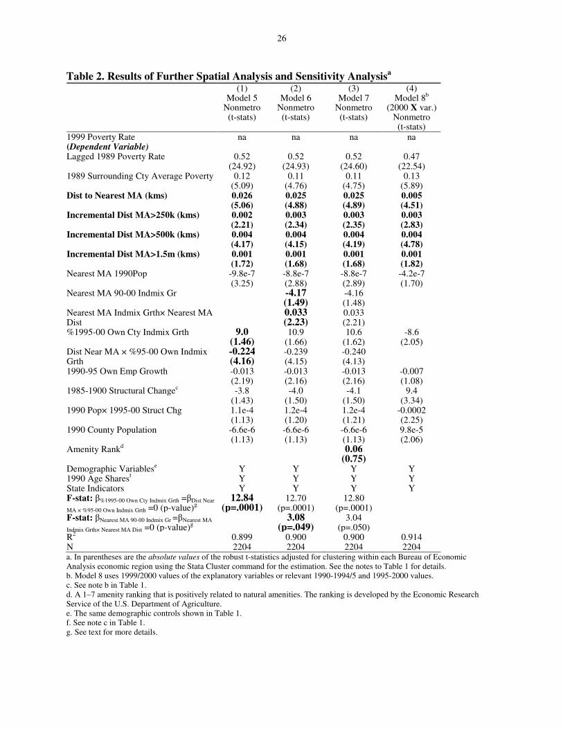
4.2 Further Analysis of Spatial Effects and Examination of Robustness

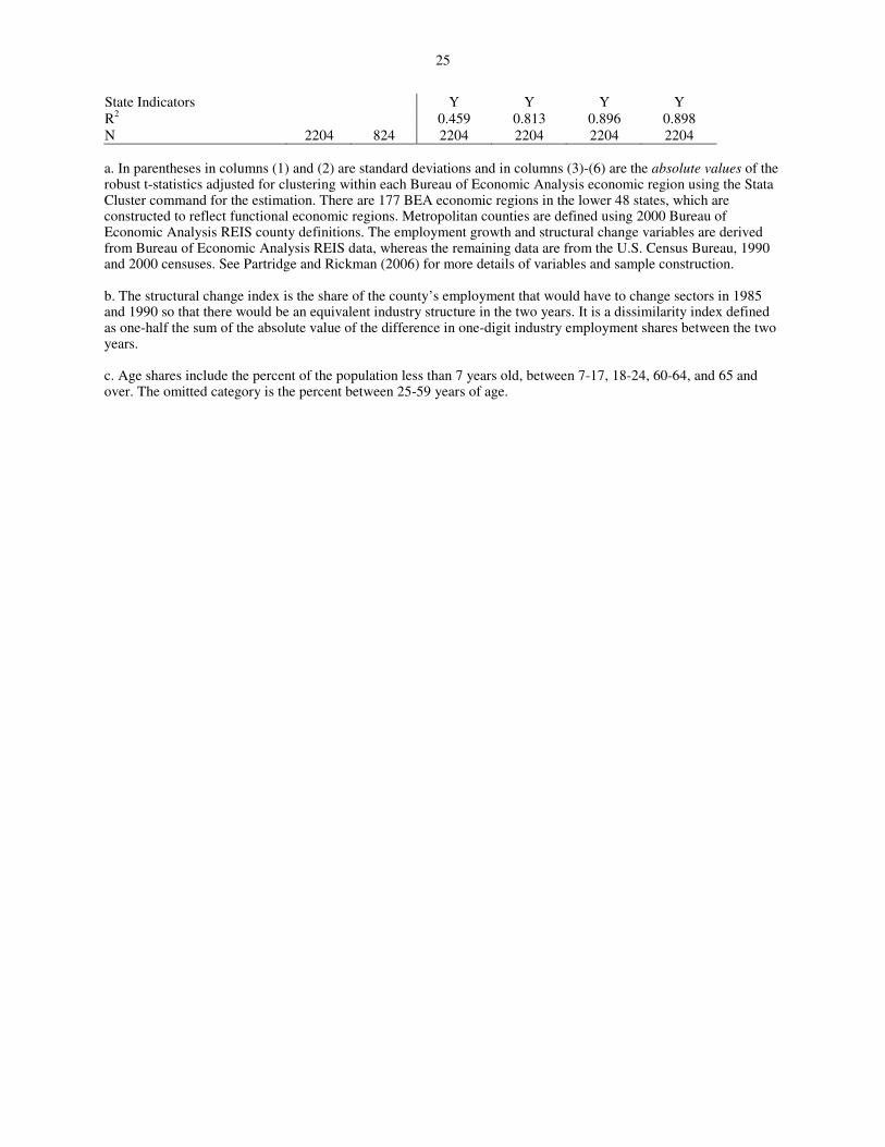
Table 2 reports the results of further analysis of the spatial effects and sensitivity analysis. To

investigate if the significance of the distance variables partly relates to commuting and migration

responses to labor demand shifts, we add to Model 4 the interaction of distance to the nearest MA area

with the nonmetropolitan county’s 1995-2000 industry mix growth, producing Model 5. The distance-

industry mix interaction coefficient, shown in bold font, is negative, which is consistent with our

hypothesis described above that job growth reduces poverty more when the county is farther from its

nearest urban center. In addition, the F-statistic reported at the bottom of Table in bold font indicates that

the two own-county industry mix growth variables are jointly highly significant. Using the mean value for

19

Note that the difference in the magnitude of the coefficients partially reflects that actual 1990-95 employment growth and 1995-2000 industry mix growth are respectively measured as percentage change and rate of change.

20In the calculation, we included the marginal effects of the incremental distance to reach a MA of at least 1.5

million even though it was only significant at the 15% level because in subsequent models in Table 2, it is significant at the 10% level.

16

own-county industry mix employment growth, it begins to reduce poverty at a distance of about 40 km

from the nearest MA. In addition, the magnitudes of the PROXIMITY variable coefficients generally

increase and statistical significance improves.

We also examine more specifically whether urban employment growth spreads to the countryside,

such as through producing job opportunities for the rural poor. This hypothesis differs from whether basic

urban proximity affects rural county poverty rates because the proximity variables did not account for

whether the most-proximate urban centers are growing, which creates more job opportunities. We

consider this possibility by adding to Model 5 the 1990-2000 industry mix growth rate in the nearest MA

and an interaction of this variable with distance to the nearest MA, producing model 6, with the new

variable shown in bold.21

Although the 1990-2000 nearest MA industry mix employment growth variable

is only statistically significant at the 15% level, the F-statistic reported in bold at the bottom of the table

indicates that the two MA employment variables are jointly statistically significant at the 5% level.

The coefficients suggest that urban “spread” effects reduce rural poverty, in which one likely

avenue is through creating job-commuting opportunities. A one standard deviation increase in the nearest

MA industry mix growth rate is associated with a -0.3 percentage points decrease in a rural county’s

poverty rate if it is immediately adjacent to the core of the urban center. However, at the mean distance of

90kms, the corresponding change in poverty is only -0.1 percentage points. Yet, illustrating that urban

proximity has other channels of influence on rural poverty, the distance variable coefficients are virtually

unchanged in this model compared to Model 5.

In interpreting our results, one of our key hypotheses is that reduced migration responses to labor

demand shifts in more remote areas cause labor supply to be more inelastic. To further examine this

hypothesis, we perform an additional regression, which specifies the percent of residents in the county in

2000 who were residents five years previously as the dependent variable. This variable is an inverse

measure of recent migration and is a direct measure of the number of “original residents.” The greater the

migration response to employment growth, the smaller will be share of the population in 2000 who lived

in the same county in 1995. Specifically, we regress this share on the 1990-2000 industry mix

21

We use the metropolitan industry mix growth rate to mitigate any endogeneity concerns from using the actual MA employment growth rate. As with own-county growth, MA growth over the entire 1990s is used to allow for the possibility that it may take especially prolonged growth to trickle out to the rural areas and reduce poverty.

17

employment growth variable, its interaction with distance, and state fixed effects.

In results not shown, consistent with expectations, we find the share of the population in 2000 who

resided in the county in 1995 to be negatively related to our measure of labor demand, indicating greater

(smaller) net in- (out-) migration when local economic conditions are stronger (weaker). Yet, consistent

with our hypothesis, this effect attenuates with distance. The interaction of industry mix employment

growth and distance is positive and statistically significant (p-value=.05), indicating reduced migration

responses (a larger share of original residents) the farther the county was from its nearest metropolitan

area. Hence, the results support our argument that higher poverty in more remote areas occurs at least

partly because of smaller labor supply adjustments(through smaller migration responses) to negative labor

demand shifts, and does not simply reflect a preference for living in more remote areas.

We also examined whether the type of local county job growth affected the results. For example, the

retail sector and rural manufacturing may be two sectors that are more conducive for low-skilled workers

to obtain employment. To consider this possibility, we re-estimated the specifications in Model 6 by

replacing the own-county 1990-1995 and 1995-2000 growth in total employment with the growth in retail

employment (including the retail employment growth × distance to nearest MA interaction). Then we

repeat but substituting manufacturing employment growth for total employment growth.22

These results

(not shown) suggest that neither own-county retail employment growth nor its interaction with distance to

the nearest MA is statistically significant, which is also the case for the manufacturing results. These

models suggest that overall employment growth is a better measure of job availability for low-skilled

workers in rural areas than retail and manufacturing job growth (at least for our specification).23

In another sensitivity test we assess whether a county’s natural amenities correlate with the

PROXMITY variables and the poverty rate. To assess this possibility, the USDA natural amenity

22

We use the 1995-2000 own-county industry mix as an instrument for 1995-2000 retail and manufacturing employment growth (industry mix growth interacted with distance to the nearest MA is also used as an instrument). 23

We also considered whether job growth had different effects in farm dependent counties and in manufacturing dependent counties after dividing the sample based on the 1993 U.S. Department of Agriculture, Economic Research Service typology. These results suggested that for the 531 farm dependent county sample, proximity to nearby MAs have moderately stronger effects than in the entire sample, while own-county employment growth had modestly greater poverty-reducing impacts in more distant farm-dependent counties. Conversely, employment growth in the nearest MA had a statistically insignificant effect that differed from the entire sample. For the 501 manufacturing dependent counties, compared to the entire sample, poverty rates appeared to be less affected by the direct effects of proximity to larger MAs, while own-county employment growth had a smaller influence as well. Alternatively, job growth in the nearest MA had larger spread effects than the entire sample. Thus, there appears to be modest differences across different rural types. See Partridge and Rickman’s (2007) geographically weighted regression analysis for a fuller investigation of spatial heterogeneity across counties.

18

measure is added to Model 6, forming Model 7. However, the amenity measure is insignificant in this

model and the other results are essentially unchanged.

In a final sensitivity test, Column (4) reports the results of Model 8, which, except for the

employment growth variables, replaces the explanatory variables in Model 4 measured in the 1980s and

1990 with corresponding variables measured in the 1990s and 2000. This specification assesses whether

changes in the explanatory variables during the 1990s underlie some of the key results, or alternatively,

whether endogeneity is affecting the results. However, except for population of the nearest MA, whose

coefficient declined by about one-half, the PROXIMTY variable coefficients are similar using more

contemporaneous control variables. The similarity between the distance results using 1990 or 2000

control variables further suggests that even in the more fully specified models, those results are not

meaningfully affected by possible endogeneity bias.

5. Summary and Conclusions

Using a novel approach for representing rural proximity, we examined the nexus between poverty in

rural counties and their geographical location within the urban hierarchy. We found ceteris paribus

increases in rural poverty rates the more distant an area was from a metropolitan area. Furthermore,

higher poverty rates were found for increased incremental distances from metropolitan areas in each

successively higher (larger) population tier.

We argue that the positive link between rural remoteness and poverty occurs because of the

attenuation of agglomeration benefits over distance and incomplete/smaller labor supply responses,

producing a form of rural spatial mismatch. For example, distance may inhibit rural trade of goods with

MAs, reduce job-commuting opportunities for rural residents, and reduce access to specialized urban

services, which serve to decrease demand for rural workers. And combined with incomplete labor supply

responses, greater distance produces significantly higher poverty results in remote rural areas ─ even after

accounting for spatial differences in demographics, natural amenities, and other attributes.

In additional analysis, job growth in the nearest MA was found to have favorable poverty-reducing

impacts that attenuate with greater distance. Thus, some of the antipoverty benefits of close proximity to

metropolitan areas relate to “spread” effects such as increased job-commuting opportunities. We also

found that local employment growth has greater poverty-reducing impacts in remote counties. This likely

19

occurs because of smaller commuting and migration flows between remote areas and other areas; i.e.,

remote areas have a more inelastic labor supply. To be sure, in further analysis, we find more direct

evidence of incomplete supply-side adjustment to demand shifts in more remote areas, suggesting higher

poverty in these areas does not simply reflect a greater desire to live in remote areas. Correspondingly, we

found rural poverty to be unaffected by a measure of the area’s amenity attractiveness.

So, although market forces appear to inhibit labor demand in remote areas, because of inter-

regionally incomplete supply responses to demand shifts, geographically-targeted policy efforts to

stimulate growth may produce larger antipoverty benefits (Bigman and Fofack, 2000; Partridge and

Rickman, 2005). In this sense, remoteness is an advantage because local job growth benefits more

original residents rather than nonresident in-commuters and new in-migrants. But the strong market forces

pulling growth to areas more proximate to larger urban centers may be too costly to overcome.

One long-term antipoverty policy might simply consist of urbanization trickle down, in which

improved access to urban labor markets reduces rural poverty (which is reinforced by stronger urban

growth). Because of limited labor mobility, place-based economic development can also be a complement

to fight poverty in remote regions along with people-based policies such as augmenting the skills of low-

skilled workers. In addition, if automobile ownership is low in remote regions (Beale, 2004) funding

grants for the poor to purchase an automobile may increase out-commuting and reduce the poverty

impacts in declining regions. Likewise, funding could be provided for childcare centers in remote areas

where they are sparse (Weber, Duncan and Whitener, 2001; Mills and Hazarika, 2003), which also could

provide residents increased ability to take more distant jobs. Thus, remoteness should not only be

examined for its effects on rural poverty, but the underlying factors contributing to remoteness being

associated with higher poverty should be identified in the design of rural antipoverty policies.

References

Bartik, Timothy J., 1991. Who Benefits from State and Local Economic Development Policies? Kalamazoo, Mich.: W. E. Upjohn Institute for Employment Research. ______, 1993. "Who Benefits from Local Job Growth: Migrants or the Original Residents," Regional Studies 27 (1993), 297-311. Beale, C.L. 2004. “Anatomy of Nonmetro High Poverty Areas: Common in Plight Distinctive in Nature,” Amber Waves 2(5), available at http://www.ers.usda/AmberWaves/AllIssues/.

20

Bigman, David and Hippolyte Fofack, 2000. “Geographical Targeting for Poverty Alleviation: An Introduction to the Special Issue,” World Bank Review 14(1), 129-145. Blanchard, Olivier J. and Lawrence F. Katz, 1992. “Regional Evolutions,” Brookings Papers on Economic Activity (1), 1-75. Blumenberg, Evelyn and Kimiko Shiki, 2004. “Spatial Mismatch Outside of Large Urban Areas: An Analysis of Welfare Recipients in Fresno County, California,” Environment and Planning C: Government and Policy 22, 401-421. Borjas, George J., 2003. “The Labor Demand Curve Is Downward Sloping: Reexamining the Impact of Immigration on the Labor Market,” Quarterly Journal of Economics 118(4), 1335-74. Bound, John and Harry J. Holzer, 2000. “Demand Shifts, Population Adjustments, and Labor Market Outcomes in the 1980s,” Journal of Labor Economics 18, 20-54. Davis, Elizabeth E. and Bruce A. Weber, 2002. “How Much Does Local Job Growth Improve Employment Outcomes of the Rural Working Poor?” The Review of Regional Studies 32(2), 255-274. Dekle and Jonathan Eaton, 1999. “Agglomeration and Land Rents: Evidence from the Prefectures,” Journal of Urban Economics 46(2), 200-214. Fisher, Monica, 2005. “On the Empirical Finding of a Higher Risk of Poverty in Rural Areas: Is Rural Residence Endogenous to Poverty? Journal of Agricultural and Resource Economics 30(2), 185-99. _____, 2007. Why Is U.S. Poverty Higher in Nonmetropolitan than in Metropolitan Areas? Growth and Change 38(1), 56-76. Freeman, Richard, 2001. “The Rising Tide Lifts…?” In Understanding Poverty, Sheldon H. Danziger and Robert Haveman, eds. Cambridge, MA: Harvard University Press pp.97-126. Fujita, Masahisa, Paul Krugman, and Tomoya Mori, 1999. “On the Evolution of Hieracrchical Urban Systems,” European Economic Review 43, 209-251. Gibbs, Robert M., 1994. “The Information Effects of Origin on Migrants’ Job Search Behavior,” Journal of Regional Science 34, 163-178. Glaeser, Edward L., 1997. Are Cities Dying? Journal of Economic Perspectives 12(2), 139-60. Glasmeier, A.K and T.L. Farrigan. 2003. “Poverty Sustainability and the Culture of Despair: Can Sustainable Development Strategies Support Poverty Alleviation in America’s Most Environmentally Challenged Communities.” The Annals of the American Academy of Political and Social Science 590, 131-149. Gundersen, C. and J.P. Ziliak, 2004. “Poverty and Macroeconomic Performance across Space, Race, and Family Structure,” Demography 41(1), 61-86.

Gyourko, J. and J. Tracy, 1989. “The Importance of Local Fiscal Conditions when Analyzing Local Labor Markets,” Journal of Political Economy 97, 1208-1231. Hanson, Gordon H., 1997. “Increasing Returns, Trade and the Regional Structure of Wages,” Economic Journal 107, 113-33. _____, 1998. “Market Potential, Increasing Returns, and Geographic Concentration.” NBER Working Paper # 6429.

21

_____, 2005. “Market Potential, Increasing Returns and Geographic Concentration,” Journal of International Economics 67, 1-24. Henderson, J. Vernon and Hyoung Gun Wang, 2005. “Aspects of the Rural-Urban Transformation of Countries,” Journal of Economic Geography 5, 23-42. Henry, M.S., Barkley, D.L. and Bao, S, 1997. “The Hinterland’s Stake in Metropolitan Area Growth,” Journal of Regional Science 37 (3), 479-501. Henry, M.S., B. Schmitt, and V. Piguet, 2001. “Spatial Econometric Models for Simultaneous Systems: Application to Rural Community Growth in France,” International Regional Science Review 24 (2), 171-93. Hines, James R. Jr., Hilary Hoynes and Alan B. Krueger, 2001. “Another Look as Whether a Rising Tide Lifts All Boats,” NBER Working Paper 8412, http://www.nber.org/papers/w8412. Houston, Donald, 2005. “Methods to Test the Spatial Mismatch Hypothesis,” Economic Geography 81(4), 407-434. Hoynes, Hilary W., Marianne E. Page and Ann H. Stevens, 2006. “Poverty in America: Trends and Explanations,” NBER Working Paper 11681, http://www.nber.org/papers/w11681. Johnson, Rucker C., 2006. “Landing a Job in Urban Space: The Extent and Effects of Spatial Mismatch,”

Regional Science and Urban Economics 36, 331-372. Krugman, Paul, 1993. “First Nature, Second Nature, and Metropolitan Location,” Journal of Regional Science 33, 129-144.

Levernier, W., M.D. Partridge, and D.S. Rickman, 2000. “The Causes of Regional Variations in U.S. Poverty: A Cross-County Analysis,” Journal of Regional Science 40, 473-98. Lucas, Robert E.B, 2001. “The effects of proximity and transportation on developing country population migrations.” Journal of Economic Geography 1, 323-339. Madden, J.F., 1996. “Changes in the Distribution of Poverty across and within the US Metropolitan Areas, 1979-89,” Urban Studies 33, 1581-1600. Mills, B.F., and G. Hazarika. 2003. Do Single Mothers Face Greater Constraints to Workforce Participation in Non-metropolitan Areas? American Journal of Agricultural Economics 85(1): 143-61. Molho, Ian, 1995. “Migrant Inertia, Accessibility and Local Unemployment,” Economica 62, 123-132. Nord, Mark, 1998. “Poor People on the Move: County-to-County Migration and the Spatial Concentration of Poverty,” Journal of Regional Science 38(2), 329-51. Nord, Mark and Ephraim Leibtag, 2005.“ Is the ‘Cost of Enough Food’ Lower in Rural Areas?” The Review of Regional Studies 35(3), 291-310. Overman, Henry G. and Yannis M. Ioannides, 2001. “Cross-Sectional Evolution of the U.S. City Size Distribution,” Journal of Urban Economics 49, 543-566. Partridge, Mark D. and Dan S. Rickman, 2003. “The Waxing and Waning of Regional Economies: The Chicken-Egg Question of Jobs versus People,” Journal of Urban Economics, 53(1), 76-97. _____, 2005. “Persistent High-Poverty in Nonmetropolitan America: Can Economic Development Help?”

22

International Regional Science Review 28, 415-440.

_____. 2006. The Geography of American Poverty: Is There a Role for Place-Based Policies? The W.E. Upjohn Institute for Employment Research: Kalamazoo, MI.

_____. 2007. “Persistent Pockets of Extreme American Poverty and Job Growth: Is There a Place Based Policy Role,” Journal of Agriculture and Resource Economics 32(1), 201-224. Partridge, Mark D., Ray Bollman, M. Rose Olfert, and Alessandro Alasia. 2007. “Riding the Wave of Urban Growth in the Countryside: Spread, Backwash, or Stagnation,” Land Economics, 83(2). Partridge, M.D., M.R. Olfert, and A. Alasia, 2007. “Canadian Cities as Regional Engines of Growth: Agglomeration and Amenities,” Canadian Journal of Economics 40(1), 39-68. Partridge, M.D., D.S. Rickman, K. Ali, and M.R. Olfert, 2006. “Employment Growth in the American Urban Hierarchy: Long Live Distance.” unpublished manuscript available at www.bus.okstate.edu/ecls/rickman/emp_distance.pdf. Partridge, M.D., D.S. Rickman, K. Ali, and M.R. Olfert, forthcoming. “The Geographic Diversity of U.S. Nonmetropolitan Growth Dynamics: A Geographically Weighted Regression Approach,” Land Economics 84(2). Ravallion, Martin and Quentin Wodon, 1999. “Poor Areas, or Only Poor People,” Journal of Regional Science 39(4), 689-711. Rosenthal, Stuart S. and William C. Strange, 2001. “The Determinants of Agglomeration,” Journal of Urban Economics, 50, 191-229. _____, 2003. “Geography, Industrial Organization, and Agglomeration,” Review of Economics and

Statistics 85(2), 377-93. _____, 2005. “The Attenuation of Human Capital Spillovers” unpublished manuscript. Accessed at

http://www.rotman.utoronto.ca/~wstrange/Rosenthal_Strange_Wage_11-29-06.pdf. Swaminathan, Hema and Jill L. Findeis, 2004. “Policy Intervention and Poverty in Rural America,” American Journal of Agricultural Economics 86(5), 1289-1296. U.S. Census Bureau, 2006. Current Population Survey: Table 2 of Historical Poverty Tables. http://www.census.gov/hhes/www/poverty/histpov/hstpov2.html accessed August 4, 2006. U.S. Department of Agriculture, 2006. ERS/USDA Briefing Room: Rural Population and Migration: Rural Population Change and Net Migration. http://www.ers.usda.govBriefing/Population/PopChange/, accessed June 29, 2006. U.S. General Accounting Office, 1995. Poverty Measurement: Adjusting for Geographic Cost-of-Living Differences. GAO/GGD-95-64. U.S. General Accounting Office: Washington D.C. van Soest, Daan P., Shelby Gerking, Shelby and Frank G. van Oort, 2006. “Spatial Impacts of Agglomeration Externalities,” Journal of Regional Science 46(5), 881-99. Venables, A.J., 1996. “Equilibrium Locations of Vertically Linked Industries,” International Economic Review 37, 341-59.

Weber, B.A., G.J. Duncan, and L.A. Whitener. 2001. Welfare Reform in Rural America: What Have We Learned. American Journal of Agricultural Economics 83(5): 1282-1292.

23

Weber, Bruce, Leif Jensen, Kathleen Miller, Jane Mosely and Monica Fisher, 2005. “Critical Review of Rural Poverty Literature: Is There Truly a Rural Effect?” International Regional Science Review 28(4), 381-414.

24

Table 1. Descriptive Statistics and Base Regression Resultsa

(1)

Nonmetro

Counties

(std dev)

(2)

Metro

Counties

(std dev)

(3)

Model 1

Nonmetro

(t-stats)

(4)

Model 2

Nonmetro

(t-stats)

(5)

Model 3

Nonmetro

(t-stats)

(6)

Model 4

Nonmetro

(t-stats)

1999 Poverty Rate

(Dependent Variable)

15.3

(6.6)

11.0

(4.8)

na na na na

Lagged 1989 Poverty Rate

18.4

(7.9)

12.3

(5.6)

0.52

(22.78)

0.53

(24.79)

1989 Surrounding Cty

Average Poverty

17.8

(6.4)

13.7

(5.4)

0.12

(5.18)

0.12

(4.91)

Dist to Nearest MA (kms) 89.9

(58.5)

na 0.019

(4.44)

0.013

(5.60)

0.006

(5.36)

0.005

(4.63)

Incremental Dist MA>250k

(kms)

65.7

(103.4)

na 0.006

(1.69)

0.003

(2.02)

0.003

(2.64)

0.002

(2.18)

Incremental Dist MA>500k

(kms)

43.2

(67.7)

na 0.017

(4.65)

0.011

(5.65)

0.005

(4.39)

0.004

(4.05)

Incremental Dist MA>1.5m

(kms)

91.0

(114.7)

na 0.006

(1.94)

0.003

(1.95)

0.001

(1.77)

0.001

(1.49)

Nearest MA 1990Pop 149,033

(135,727)

na -1.8e-6

(2.48)

-1.4e-6

(2.82)

-1.0e-6

(3.29)

-9.2e-7

(3.12)

Nearest MA 90-00 Indmix Gr 0.168

(0.063)

na

%1995-00 Own Cty Indmix

Grth

0.095

(0.018)

0.115

(0.02)

-12.8

(3.08)

1990-95 Own Emp Growth

10.4

(19.5)

12.4

(11.0)

-0.012

(1.88)

1985-1990 Structural Changeb

0.070

(0.03)

0.060

(0.02)

-3.2

(1.20)

1990 Pop× 1995-00 Struct Chg

na na 9.5e-5

(0.98)

1990 County Population

22,416

(20,746)

239,597

(478,619)

-1.5e-5

(2.45)

-2.1e-5

(4.50)

1.4e-6

(0.43)

-3.9e-6

(0.70)

% Population that immigrated

between 1985-1990

0.3

(0.7)

0.9

(1.4)

-0.01

(0.04)

0.17

(1.08)

0.13

(0.80)

% Population that immigrated

between 1980-1984

0.2

(0.6)

0.6

(1.1)

-0.09

(0.27)

0.09

(0.41)

0.17

(0.75)

1990 %Not HS Graduate

(age≥ 25yrs)

32.5

(10.3)

25.1

(8.2)

1990 %HS Graduate

(age≥ 25yrs)

35.1

(5.9)

32.5

(6.2)

-0.43

(7.73)

-0.13

(6.07)

-0.12

(6.16)

1990 %Some College, no

degree (age≥ 25yrs)

15.6

(4.4)

18.4

(4.1)

-0.33

(6.65)

-0.05

(1.79)

-0.03

(0.99)

1990 %Associate College

Degree (age≥ 25yrs)

5.1

(2.2)

6.0

(1.7)

-0.44

(5.79)

-0.10

(2.09)

-0.10

(2.17)

1990 %Bachelors Degree or

more (age≥ 25yrs)

11.7

(4.8)

18.1

(7.9)

-0.20

(6.34)

-0.06

(3.23)

-0.03

(1.55)

1990 % of HHs female-headed

with children

5.2

(2.4)

5.9

(1.8)

0.69

(9.13)

0.12

(2.10)

0.13

(2.45)

1990 % of HHs male-headed

with children

1.4

(0.6)

1.3

(0.4)

0.28

(1.65)

-0.05

(0.36)

-0.005

(0.04)

1990%Pop African American

8.2

(15.1)

9.8

(11.8)

0.05

(2.83)

0.02

(2.15)

0.017

(1.81)

1990 %Pop Other Race

(non Caucasian, Black)

3.8

(8.0)

4.0

(5.6)

0.12

(3.79)

0.06

(2.81)

0.06

(2.91)

1990 %Pop Hispanic

4.2

(11.4)

4.7

(9.7)

0.007

(0.35)

-0.02

(1.26)

-0.02

(1.41)

1990 Age Sharesc

N Y Y Y

25

State Indicators

Y Y Y Y

R2

0.459 0.813 0.896 0.898

N 2204 824 2204 2204 2204 2204

a. In parentheses in columns (1) and (2) are standard deviations and in columns (3)-(6) are the absolute values of the robust t-statistics adjusted for clustering within each Bureau of Economic Analysis economic region using the Stata Cluster command for the estimation. There are 177 BEA economic regions in the lower 48 states, which are constructed to reflect functional economic regions. Metropolitan counties are defined using 2000 Bureau of Economic Analysis REIS county definitions. The employment growth and structural change variables are derived from Bureau of Economic Analysis REIS data, whereas the remaining data are from the U.S. Census Bureau, 1990 and 2000 censuses. See Partridge and Rickman (2006) for more details of variables and sample construction. b. The structural change index is the share of the county’s employment that would have to change sectors in 1985 and 1990 so that there would be an equivalent industry structure in the two years. It is a dissimilarity index defined as one-half the sum of the absolute value of the difference in one-digit industry employment shares between the two years. c. Age shares include the percent of the population less than 7 years old, between 7-17, 18-24, 60-64, and 65 and over. The omitted category is the percent between 25-59 years of age.

26

Table 2. Results of Further Spatial Analysis and Sensitivity Analysisa

(1) Model 5

Nonmetro (t-stats)

(2) Model 6

Nonmetro (t-stats)

(3) Model 7

Nonmetro (t-stats)

(4) Model 8

b

(2000 X var.) Nonmetro (t-stats)

1999 Poverty Rate (Dependent Variable)

na na na na

Lagged 1989 Poverty Rate

0.52 (24.92)

0.52 (24.93)

0.52 (24.60)

0.47 (22.54)

1989 Surrounding Cty Average Poverty 0.12 (5.09)

0.11 (4.76)

0.11 (4.75)

0.13 (5.89)

Dist to Nearest MA (kms) 0.026 (5.06)

0.025 (4.88)

0.025 (4.89)

0.005 (4.51)

Incremental Dist MA>250k (kms) 0.002 (2.21)

0.003 (2.34)

0.003 (2.35)

0.003 (2.83)

Incremental Dist MA>500k (kms) 0.004 (4.17)

0.004 (4.15)

0.004 (4.19)

0.004 (4.78)

Incremental Dist MA>1.5m (kms) 0.001 (1.72)

0.001 (1.68)

0.001 (1.68)

0.001 (1.82)

Nearest MA 1990Pop -9.8e-7 (3.25)

-8.8e-7 (2.88)

-8.8e-7 (2.89)

-4.2e-7 (1.70)

Nearest MA 90-00 Indmix Gr -4.17 (1.49)

-4.16 (1.48)

Nearest MA Indmix Grth× Nearest MA Dist

0.033 (2.23)

0.033 (2.21)

%1995-00 Own Cty Indmix Grth 9.0 (1.46)

10.9 (1.66)

10.6 (1.62)

-8.6 (2.05)

Dist Near MA × %95-00 Own Indmix Grth

-0.224 (4.16)

-0.239 (4.15)

-0.240 (4.13)

1990-95 Own Emp Growth

-0.013 (2.19)

-0.013 (2.16)

-0.013 (2.16)

-0.007 (1.08)

1985-1900 Structural Changec

-3.8

(1.43) -4.0

(1.50) -4.1

(1.50) 9.4

(3.34) 1990 Pop× 1995-00 Struct Chg

1.1e-4 (1.13)

1.2e-4 (1.20)

1.2e-4 (1.21)

-0.0002 (2.25)

1990 County Population

-6.6e-6 (1.13)

-6.6e-6 (1.13)

-6.6e-6 (1.13)

9.8e-5 (2.06)

Amenity Rankd

0.06

(0.75)

Demographic Variablese

Y Y Y Y 1990 Age Shares

f Y Y Y Y

State Indicators

Y Y Y Y F-stat: β%1995-00 Own Cty Indmix Grth =βDist Near

MA × %95-00 Own Indmix Grth =0 (p-value)g

12.84 (p=.0001)

12.70 (p=.0001)

12.80 (p=.0001)

F-stat: βNearest MA 90-00 Indmix Gr =βNearest MA

Indmix Grth× Nearest MA Dist =0 (p-value)g

3.08 (p=.049)

3.04 (p=.050)

R2

0.899 0.900 0.900 0.914 N 2204 2204 2204 2204 a. In parentheses are the absolute values of the robust t-statistics adjusted for clustering within each Bureau of Economic

Analysis economic region using the Stata Cluster command for the estimation. See the notes to Table 1 for details.

b. Model 8 uses 1999/2000 values of the explanatory variables or relevant 1990-1994/5 and 1995-2000 values.

c. See note b in Table 1.

d. A 1–7 amenity ranking that is positively related to natural amenities. The ranking is developed by the Economic Research

Service of the U.S. Department of Agriculture.

e. The same demographic controls shown in Table 1.

f. See note c in Table 1.

g. See text for more details.